Properties of the Strong Data Processing Constant for Rényi Divergence

Abstract

Strong data processing inequalities (SDPI) are an important object of study in Information Theory and have been well studied for $f$-divergences. Universal upper and lower bounds have been provided along with several applications, connecting them to impossibility (converse) results, concentration of measure, hypercontractivity, and so on. In this paper, we study Rényi divergence and the corresponding SDPI constant whose behavior seems to deviate from that of ordinary $\Phi$-divergences. In particular, one can find examples showing that the universal upper bound relating its SDPI constant to the one of Total Variation does not hold in general. In this work, we prove, however, that the universal lower bound involving the SDPI constant of the Chi-square divergence does indeed hold. Furthermore, we also provide a characterization of the distribution that achieves the supremum when $\alpha$ is equal to $2$ and consequently compute the SDPI constant for Rényi divergence of the general binary channel.

I Introduction

The well-known data processing inequality (DPI) for relative entropy states that, for any two probability distributions $\mu,\nu$ such that $\nu\ll\mu$ over an alphabet $\mathcal{X}$ and for any stochastic transformation $K$ with input alphabet $\mathcal{X}$ and output alphabet $\mathcal{Y}$, we have

$$D_{\text{KL}}(\nu K||\mu K)\leq D_{\text{KL}}(\nu||\mu),$$ (1)

where $D_{\text{KL}}(\nu||\mu)$ is the KL-divergence between $\nu,\mu$. However, this inequality can be improved if we fix $\mu,K$ and only let $\nu$ vary. Indeed, one can have that for every $\nu$, unless $\nu=\mu$. $D_{\text{KL}}(\nu K||\mu K)$ is strictly less than $D_{\text{KL}}(\nu||\mu)$. Formally, one can define the Strong Data Processing Inequality (SDPI) constant of the KL-divergence for $\mu,K$ as in [1, 2, 3]

$$\eta_{\text{KL}}(\mu,K):=\sup_{\nu\neq\mu}\dfrac{D_{\text{KL}}(\nu K||\mu K)}{D_{\text{KL}}(\nu||\mu)}.$$ (2)

Moreover, $\Phi$-divergences, a well-known generalization of the KL-divergence [4, 5], also allow for the definition of a corresponding SDPI constant. Thus, consider a convex function $\Phi:\mathbb{R}^{+}\to\mathbb{R}$ such that $\Phi(1)=0$ and two probability distributions $\nu\ll\mu$, one can define the $\Phi$-divergence as follows

$$D_{\Phi}(\nu\|\mu)=\mathbb{E}_{\mu}\left[\Phi\left(\frac{d\nu}{d\mu}\right)\right]$$ (3)

and, given a Markov kernel $K$, the corresponding SDPI constant as follows:

$$\eta_{\Phi}(\mu,K) :=\sup_{\nu:\nu\neq\mu}\dfrac{D_{\Phi}(\nu K\|\mu K)}{D_{\Phi}(\nu\|\mu)},$$ (4)

$$\eta_{\Phi}(K) :=\sup_{\mu\in\mathcal{P}(\mathcal{X})}\eta_{\Phi}(\mu,K),$$ (5)

where $\mathcal{P}(\mathcal{X})$ is the set of all the probability distributions over $\mathcal{X}$. These objects have been connected to several others, such as the maximal correlation and the so-called hypercontractivity constants of certain Markov operators [6, 7]. Moreover, given the importance of the Data Processing Inequality in Information Theory and the possibility of improving the corresponding results computing the SDPI constants, they have gained increasing interest over the years, leading to a variety of applications, universal upper and lower bounds [8, 9, 2]. In particular, it is known that for any $\Phi$ and any channel $K$ [2, Theorem 3.1]

$$\eta_{\Phi}(K)\leq\eta_{\text{TV}}(K),$$ (6)

while if $\Phi$ is also three times differentiable, given any measure $\mu$ [2, Theorem 3.3]:

$$\eta_{\Phi}(\mu,K)\geq\eta_{\chi^{2}}(\mu,K),\eta_{\Phi}(K)\geq\eta_{\chi^{2}}(K).$$ (7)

$\eta_{\text{TV}}$ and $\eta_{\chi}^{2}$ denote the SDPI constant of the divergences induced, respectively, by $\Phi(x)=\frac{1}{2}|x-1|$ and $\Phi(x)=x^{2}-1$.

Rényi divergences $D_{\alpha}$ represents another family of divergences that are known to satisfy the DPI and lend themselves to the definition of a corresponding SDPI constant but that do not belong to the family of $\Phi$-divergences. The Rényi divergence $D_{\alpha}(\nu||\mu)$ of two probability distributions $\nu\ll\mu$ for $\alpha\not\in\{0,1,\infty\}$ can be defined as follows [10]

$$D_{\alpha}(\nu\|\mu):=\dfrac{1}{\alpha-1}\log\mathbb{E}_{\mu}\left[\left(\dfrac{\mathrm{d}\nu}{\mathrm{d}\mu}\right)^{\alpha}\right].$$ (8)

Moreover, one can define the corresponding SDPI constant

$$\eta_{\alpha}(\mu,K) :=\sup_{\nu:\nu\neq\mu}\dfrac{D_{\alpha}(\nu K\|\mu K)}{D_{\alpha}(\nu\|\mu)},$$ (9)

$$\eta_{\alpha}(K) :=\sup_{\mu\in\mathcal{P}(\mathcal{X})}\eta_{\alpha}(\mu,K).$$ (10)

To the best of our knowledge, the SDPI constant for Rényi divergence has been rarely investigated. Unlike the SDPI constant for $\Phi$-divergence, it does not seem to satisfy the classical upper bound highlighted in [2]. [11, Example 2] shows that it can hold $\eta_{\alpha}>\eta_{\text{TV}}$, thus violating Eq. (6). However, it is not known whether the universal lower bound $\eta_{\chi^{2}}\leq\eta_{\alpha}$ also fails to hold. The SDPI constant of Rényi divergence stands as an interesting object of study. Indeed, it can be proven to be related to the log-Sobolev inequality and hypercontractivity of certain types of operators [12]. Characterizing it can lead to improved concentration results for non-independent random variables [11] and improved lower bounds on the Bayesian risk in estimation procedures with privatized samples [13, Section 3.1]. Moreover, the limiting behavior of the Rényi divergence could provide new characterizations of $\eta_{\text{KL}}$, since we have by [10, Theorem 5] that $D_{\text{KL}}(\nu||\mu)=\lim\limits_{\alpha\downarrow 1}D_{\alpha}(\nu||\mu).$

In this paper, we study said object. Notably, we can prove that the universal lower-bound does indeed hold and thus

$$\eta_{\alpha}(K)\geq\eta_{\chi^{2}}(K).$$ (11)

Moreover, we study some properties of $\eta_{\alpha}$ when $\alpha=2$ and we manage to characterize the distribution achieving the supremum in (9). We will explain why our theorems are promising with some simple but conceptually crucial examples.

II Preliminaries and Notations

We denote by $\mathcal{P}(\mathcal{X})$ the set of all probability distributions on an alphabet (or a space) $\mathcal{X}$. The set of all real-valued functions on $\mathcal{X}$ is denoted by $\mathcal{F}(\mathcal{X})$. A Markov kernel (channel) $K(y|x)\in\mathcal{M}(\mathcal{Y}|\mathcal{X})$ acts on probability distributions $\mu\in\mathcal{P}(\mathcal{X})$ by

$$\mu K(y)=\sum_{x\in\mathcal{X}}\mu(x)K(y|x),\qquad y\in\mathcal{Y}.$$ (12)

or on functions $f\in\mathcal{F}(\mathcal{X})$ by

$$Kf(x)=\sum_{y\in\mathcal{Y}}K(y|x)f(y),\qquad y\in\mathcal{Y}.$$ (13)

We say an admissible pair $(\mu,K)\in\mathcal{P}(\mathcal{X})\times\mathcal{M}(\mathcal{Y}|\mathcal{X})$ if $\mu\in\mathcal{P}_{*}(\mathcal{X})$ and $\mu K\in\mathcal{P}_{*}(\mathcal{Y})$, where $\mathcal{P}_{*}$ denotes all strictly positive distributions. For any such pair, there exists a unique channel $K^{*}\in\mathcal{M}(\mathcal{X}|\mathcal{Y})$ with the property that

$$\mathbb{E}[g(Y)Kf(Y)]=\mathbb{E}[K^{*}f(X)g(X)]$$ (14)

for all $f\in\mathcal{F}(\mathcal{X}),g\in\mathcal{F}(\mathcal{X})$. The above so-called adjoint channel can be characterized in discrete settings as follows:

$$K^{*}(x|y)=\dfrac{K(y|x)\mu(x)}{\mu K(y)}.$$ (15)

Moreover, for $f=\mathrm{d}\nu/\mathrm{d}\mu$, it holds by [2, Section 1.1 and Lemma A.1] that

$$K^{*}f=\dfrac{\mathrm{d}(\nu K)}{\mathrm{d}(\mu K)}.$$ (16)

In the following discussion of this paper, we will assume $1<\alpha<\infty$ and $\mu\in\mathcal{P}_{*}(\mathcal{X})$, $\mu K\in\mathcal{P}_{*}(\mathcal{Y})$ for $D_{\alpha}$ unless specified differently. Then it is a direct consequence that $\nu\ll\mu$ and $\nu K\ll\mu K$ for every $\nu\in\mathcal{P}(\mathcal{X})$.

III Lower bounds for the SDPI constants

In this section, we will present two different versions of the lower bound for $\eta_{\alpha}(\mu,K)$. The first one is more universal and related to $\eta_{\chi^{2}}$, which implies the same lower bound as $\eta_{\Phi}$. The second one provides a lower bound that is easy to calculate. We will show by two examples that Theorems 17 and 29 coincide in some cases. Moreover, Theorem 29 can sometimes help us identify whether $\eta_{\alpha}(\mu,K)=1.$

Theorem 1 (Lower bound, Version 1).

Given a probability distribution $\mu$ and a Markov kernel $K$, the SDPI constant for Rényi divergence satisfies the following inequality:

$$\eta_{\alpha}(\mu,K)\geq\eta_{\chi^{2}}(\mu,K).$$ (17)

Proof.

Let $\nu_{\varepsilon}=\mu+\varepsilon(\nu-\mu)$ for $0<\varepsilon<1$ and $f=\mathrm{d}\nu/\mathrm{d}\mu-1$. We could derive that

$$\left.\dfrac{\partial D_{\alpha}(\nu_{\varepsilon}||\mu)}{\partial\varepsilon}\right|_{\varepsilon=0} =\left.\dfrac{\alpha\mathbb{E}_{\mu}[(1+\varepsilon f)^{\alpha-1}f]}{(\alpha-1)\mathbb{E}_{\mu}[(1+\varepsilon f)^{\alpha}]}\right|_{\varepsilon=0}=0,$$ (18)

$$\left.\dfrac{\partial^{2}D_{\alpha}(\nu_{\varepsilon}||\mu)}{\partial\varepsilon^{2}}\right|_{\varepsilon=0} =\lim\limits_{\varepsilon\downarrow 0}\dfrac{1}{\varepsilon}\cdot\dfrac{\partial D_{\alpha}(\nu_{\varepsilon}||\mu)}{\partial\varepsilon}$$ (19)

$$=\left.\dfrac{\alpha\mathbb{E}_{\mu}[(1+\varepsilon f)^{\alpha-2}f^{2}]}{\mathbb{E}_{\mu}[(1+\varepsilon f)^{\alpha}]}\right|_{\varepsilon=0}=\alpha\mathbb{E}_{\mu}[f^{2}],$$ (20)

where Eq. (18) is by direct calculation of partial derivative, and Eq. (20) is due to the L’Hôpital’s rule. Similarly,

$$\left.\dfrac{\partial D_{\alpha}(\nu_{\varepsilon}K||\mu K)}{\partial\varepsilon}\right|_{\varepsilon=0} =0,$$ (21)

$$\left.\dfrac{\partial^{2}D_{\alpha}(\nu_{\varepsilon}K||\mu K)}{\partial\varepsilon^{2}}\right|_{\varepsilon=0} =\alpha\mathbb{E}_{\mu K}[(K^{*}f)^{2}].$$ (22)

Here $K^{*}$ is the adjoint channel of $K$. Therefore, we could apply the Taylor expansion to $D_{\alpha}(\nu_{\varepsilon}||\mu)$, which yields

$$D_{\alpha}(\nu_{\varepsilon}||\mu)=\dfrac{\alpha}{2}\mathbb{E}_{\mu}[f^{2}]\varepsilon^{2}+o(\varepsilon^{2}).$$ (23)

Likewise,

$$D_{\alpha}(\nu_{\varepsilon}K||\mu K)=\dfrac{\alpha}{2}\mathbb{E}_{\mu K}[(K^{*}f)^{2}]\varepsilon^{2}+o(\varepsilon^{2}).$$ (24)

By the definition of $\eta_{\alpha}(\mu,K)$, since $\{\nu_{\varepsilon}:\nu\neq\mu,0<\varepsilon<1\}\subseteq\{\nu:\nu\neq\mu\}$, we have

$$\eta_{\alpha}(\mu,K)\geq\sup_{\nu:\nu\neq\mu}\dfrac{D_{\alpha}(\nu_{\varepsilon}K\|\mu K)}{D_{\alpha}(\nu_{\varepsilon}\|\mu)}.$$ (25)

Therefore, we conclude that

$$\eta_{\alpha}(\mu,K) \geq\sup_{\nu:\nu\neq\mu}\dfrac{\mathbb{E}_{\mu K}[(K^{*}f)^{2}]\varepsilon^{2}+o(\varepsilon^{2})}{\mathbb{E}_{\mu}[f^{2}]\varepsilon^{2}+o(\varepsilon^{2})}$$ (26)

$$=\sup_{\nu:\nu\neq\mu}\dfrac{\mathbb{E}_{\mu K}[(K^{*}f)^{2}]+o(1)}{\mathbb{E}_{\mu}[f^{2}]+o(1)}=\eta_{\chi^{2}}(\mu,K),$$ (27)

where Eq. (27) is derived by [2, Remark 3.3]. This completes the proof. ∎

It is then immediate to see that $\eta_{\chi^{2}}$ is a universal lower bound for $\eta_{\alpha}$.

Corollary 2.

Given a Markov kernel $K$, it holds

$$\eta_{\alpha}(K)\geq\eta_{\chi^{2}}(K).$$ (28)

Proof.

Take the supremum over $\mu\in\mathcal{P}_{*}(\mathcal{X})$ on both sides of Eq. (17). ∎

Now, we shall introduce another version of the lower bound for $\eta_{\alpha}$ which, differently from the previous one, can be written in closed-form and is thus easier to compute.

Theorem 3 (Lower bound, Version 2).

Let $K$ be the kernel induced by an $n\times m$ stochastic matrix and $\mu$ be a discrete distribution on a finite alphabet $\mathcal{X}$ with $|\mathcal{X}|=n$. The Rényi entropy satisfies the following inequality:

$$\eta_{\alpha}(\mu,K)\geq\max_{1\leq i\neq\ell\leq n}\dfrac{\mu_{i}\mu_{\ell}}{\mu_{i}+\mu_{\ell}}\sum_{j=1}^{m}\dfrac{{(K_{ij}-K_{\ell j})^{2}}}{(\mu K)_{j}}.$$ (29)

Proof.

For a fixed $\nu$, define $f=\mathrm{d}\nu/\mathrm{d}\mu-1$. One could see that $\mathbb{E}_{\mu}[f]=0$. Hence,

$$\eta_{\nu}:=\dfrac{D_{\alpha}(\nu K\|\mu K)}{D_{\alpha}(\nu\|\mu)}=\dfrac{\log\mathbb{E}_{\mu K}[(1+K^{*}f)^{\alpha}]}{\log\mathbb{E}_{\mu}[(1+f)^{\alpha}]}.$$ (30)

Denote $f=[f_{1},\ldots,f_{n}]^{\top}$. We could write $f_{n}$ as

$$f_{n}=-\dfrac{1}{\mu_{n}}\sum_{r=1}^{n-1}\mu_{r}f_{r},$$ (31)

which is because $f$ has zero mean. Define the following quantities:

$$P(f) :=\mathbb{E}_{\mu K}[(1+K^{*}f)^{\alpha}]$$ (32)

$$=\sum_{j=1}^{m}(\mu K)_{j}\left(1+\sum_{\ell=1}^{n-1}\left(K^{*}_{j\ell}-\dfrac{\mu_{\ell}}{\mu_{n}}K^{*}_{jn}\right)f_{\ell}\right)^{\alpha},$$ (33)

$$Q(f) :=\mathbb{E}_{\mu}[(1+f)^{\alpha}]$$ (34)

$$=\sum_{j=1}^{n-1}\mu_{j}(1+f_{j})^{\alpha}+\mu_{n}\left(1-\dfrac{1}{\mu_{n}}\sum_{r=1}^{n-1}\mu_{r}f_{r}\right)^{\alpha}.$$ (35)

We evaluate the following derivatives, in which we denote with $\partial_{i}$ being the partial derivative of the corresponding function with respect to $f_{i}$:

$$\partial_{i}P(0) =\alpha\sum_{j=1}^{m}(\mu K)_{j}\left(K^{*}_{ji}-\dfrac{\mu_{i}}{\mu_{n}}K^{*}_{jn}\right)$$ (36)

$$=\alpha\sum_{j=1}^{m}(\mu K)_{j}\left(\dfrac{\mu_{i}}{(\mu K)_{j}}K_{ij}-\dfrac{\mu_{i}}{\mu_{n}}\dfrac{\mu_{n}}{(\mu K)_{j}}K_{nj}\right)=0,$$ (37)

$$\partial_{i}^{2}P(0) =\alpha\sum_{j=1}^{m}(\mu K)_{j}\left(K^{*}_{ji}-\dfrac{\mu_{i}}{\mu_{n}}K^{*}_{jn}\right)^{2}$$ (38)

$$=\alpha\sum_{j=1}^{m}\dfrac{\mu_{i}^{2}}{(\mu K)_{j}}\left(K_{ij}-K_{nj}\right)^{2},$$ (39)

$$\partial_{i}Q(0) =\alpha\mu_{i}-\alpha\left(\dfrac{\mu_{i}}{\mu_{n}}\right)\mu_{n}=0,$$ (40)

$$\partial_{i}^{2}Q(0) =\alpha\mu_{i}+\alpha\left(\dfrac{\mu_{i}}{\mu_{n}}\right)^{2}\mu_{n}$$ (41)

$$=\alpha\left(\mu_{i}+\dfrac{\mu_{i}^{2}}{\mu_{n}}\right).$$ (42)

Denote $\eta:=\eta_{\alpha}(\mu,K)$. Now, for some fixed $i$, if we restrict the domain of $f$ to

$$\text{Dom}_{i}(\varepsilon):=\{f:0\leq f_{i}\leq\varepsilon,f_{s}=0\text{ for }s\neq i\},$$ (43)

where $\varepsilon>0$ is small enough, then it is necessary that by the definition of $\eta$,

$$\eta\geq\dfrac{\log\mathbb{E}_{\mu K}[(1+K^{*}f)^{\alpha}]}{\log\mathbb{E}_{\mu}[(1+f)^{\alpha}]},\,f\in\text{Dom}_{i}(\varepsilon).$$ (44)

Rearranging, we obtain

$$\log P(f)-\eta\log Q(f)\leq 0.$$ (45)

It is obvious that $P(0)=Q(0)=1$. Therefore, to hold Eq. (45), it is necessary that

$$S_{1}(f):=\dfrac{\partial}{\partial f_{i}}\left(\dfrac{P(f)}{Q^{\eta}(f)}\right)\leq 0,\,f\in\text{Dom}_{i}(\varepsilon).$$ (46)

Evaluating $S_{1}(f)$ at $f=0$, by the definition of partial derivative, it yields

$$S_{1}(0) =\lim\limits_{f_{i}\downarrow 0}\left.\dfrac{1}{f_{i}}\cdot\left(\dfrac{P(f)}{Q^{\eta}(f)}-1\right)\right|_{f=0}$$ (47)

$$=\lim\limits_{f_{i}\downarrow 0}\left.\dfrac{\partial_{i}P(f)-\partial_{i}Q^{\eta}(f)}{f_{i}\cdot\partial_{i}Q^{\eta}(f)+Q^{\eta}(f)}\right|_{f=0}$$ (48)

$$=\partial_{i}P(0)-\partial_{i}Q(0)=0,$$ (49)

where Eq. (48) is due to the L’Hôpital’s rule. In order to obtain $S_{1}(f)\leq 0$ in $\text{Dom}_{i}(\varepsilon)$, it is necessary to have the second derivative being negative, which is

$$S_{2}(f):=2\dfrac{\partial^{2}}{\partial f_{i}^{2}}\left(\dfrac{P(f)}{Q^{\eta}(f)}\right)\leq 0,\,f\in\text{Dom}_{i}(\varepsilon).$$ (50)

Evaluating $S_{2}(f)$ at $f=0$, by the L’Hôpital’s rule, it yields

$$S_{2}(0)=\left.2\lim\limits_{f_{i}\downarrow 0}\dfrac{P(f)-Q^{\eta}(f)}{f_{i}^{2}\cdot Q^{\eta}(f)}\right|_{f=0}={\partial_{i}^{2}P(0)-\partial_{i}^{2}Q^{\eta}(0)},$$ (51)

and by direct calculation,

$$\partial_{i}^{2}P(0)-\partial_{i}^{2}Q^{\eta}(0)=\partial_{i}^{2}P(0)-\eta\partial_{i}^{2}Q(0),$$ (52)

where we use the fact that $\partial_{i}Q(0)=0$ and $Q^{\eta}(0)=Q^{\eta-1}(0)=1$. Therefore, $S_{2}(0)\leq 0$ is equivalent to

$$\eta \geq\dfrac{\partial_{i}^{2}P(0)}{\partial_{i}^{2}Q(0)}$$ (53)

$$=\dfrac{\alpha\sum\limits_{j=1}^{m}\dfrac{\mu_{i}^{2}}{(\mu K)_{j}}\left(K_{ij}-K_{nj}\right)^{2}}{\alpha\left(\mu_{i}+\dfrac{\mu_{i}^{2}}{\mu_{n}}\right)}$$ (54)

$$=\dfrac{\mu_{i}\mu_{n}}{\mu_{i}+\mu_{n}}\sum_{j}\dfrac{{(K_{ij}-K_{nj})^{2}}}{(\mu K)_{j}}.$$ (55)

Since $i$ is arbitrary and, indeed, one can choose any $f_{\ell}$ to be $f_{n}$ in Eq. (31), which means that $\eta$ should satisfy

$$\eta\geq\max_{1\leq i\neq\ell\leq n}\dfrac{\mu_{i}\mu_{\ell}}{\mu_{i}+\mu_{\ell}}\sum_{j=1}^{m}\dfrac{{(K_{ij}-K_{\ell j})^{2}}}{(\mu K)_{j}},$$ (56)

which is the desired result. ∎

Note that the theorem gives a lower bound that is easy to calculate compared to Theorem 17 and does not depend on $\alpha$. Therefore, one could take $\alpha\downarrow 1$ and obtain a lower bound of $\eta_{\text{KL}}(\mu,K)$.

We shall see in the following example that in the two-dimensional BSC, the lower bounds given in Theorem 17 and 29 coincide. As mentioned above, one could take $\alpha\downarrow 1$ to retrieve a classical lower bound for $\eta_{\text{KL}}$.

Example 1.

Let $\mu=\text{Ber}(1/2)$ and $K=\text{BSC}(\varepsilon)$ for $0\leq\varepsilon\leq 1/2$. We have $\mu K=\text{Ber}(1/2)$ in this case. Hence, Theorem 29 gives

$$\eta_{\alpha}(\mu,K) \geq\dfrac{1}{2}\left[(K_{11}-K_{21})^{2}+(K_{12}-K_{22})^{2}\right]$$ (57)

$$=(1-2\varepsilon)^{2}=\eta_{\chi^{2}}(\mu,K).$$ (58)

Eq. (58) is illustrated in [2, Example 3.1]. Taking $\alpha\downarrow 1$, we retrieve the well-known result described in [2, Theorem 3.3] that $\eta_{\text{KL}}(\mu,K)\geq\eta_{\chi^{2}}(\mu,K)$.

Example 2.

Theorem 29 could sometimes help us to identify whether $\eta_{\alpha}(\nu,K)=1$. Consider the following case: If there exist $i\neq\ell$, $a\neq b$ such that $K_{ia}=K_{\ell b}=1$ and $K_{ja}=K_{jb}=0$ for all $j\neq i,\ell$, then we obtain

$$\eta_{\alpha}(\mu,K)\geq\dfrac{\mu_{i}\mu_{\ell}}{\mu_{i}+\mu_{\ell}}\left(\dfrac{1}{\mu_{i}}+\dfrac{1}{\mu_{\ell}}\right)=1.$$ (59)

Thus we conclude $\eta_{\alpha}(\mu,K)=1$. Moreover, since the right hand side of Eq. (59) does not depend on $\mu$, we could further obtain $\eta_{\alpha}(K)=1$.

IV Properties of $\eta_{2}(\mu,K)$

In this section, we investigate a special case of the SDPI constant when $\alpha=2$. We have the following theorem.

Theorem 4.

Let $\mu$ be a probability distribution on a finite alphabet and $K$ be a stochastic matrix with finite dimension. Whenever $\eta_{\chi^{2}}(\nu,K)<1$, the SDPI constant $\eta_{2}(\mu,K)$ satisfies

$$\eta_{2}(\mu,K)=\sup\left\{\dfrac{D_{2}(\nu K\|\mu K)}{D_{2}(\nu\|\mu)}:\nu\neq\mu\text{ and }\prod_{j}\nu_{j}=0\right\},$$ (60)

which indicates that the supremum is achieved when at least one entry of $\nu$ is zero.

Proof.

Denote $\eta:=\eta_{2}(\mu,K)$ for simplicity. We formulate $\eta$ into an optimization problem as follows.

$$\max_{\nu_{i}}\qquad \dfrac{\log\sum_{j}(\mu K)_{j}^{-1}(\nu K)_{j}^{2}}{\log\sum_{j}\mu_{j}^{-1}\nu_{j}^{2}}$$ (61)

s.t. $$\sum_{j}\nu_{j}=1.$$ (62)

Here we denote $(\mu K)_{j}$ as the $j$-th entry of the vector (distribution) $\mu K$. Define the Lagrangian function

$$G(\nu,\lambda):=\dfrac{\log\sum_{j}(\mu K)_{j}^{-1}(\nu K)_{j}^{2}}{\log\sum_{j}\mu_{j}^{-1}\nu_{j}^{2}}+\lambda\left(\sum_{j}\nu_{j}-1\right).$$ (63)

The necessary condition that an extremum should satisfy is

$$0=\dfrac{\partial G}{\partial\nu_{i}} =\dfrac{2}{\log\sum_{j}\mu_{j}^{-1}\nu_{j}^{2}}\left(\dfrac{\sum_{j}(\mu K)_{j}^{-1}(\nu K)_{j}K_{ij}}{\sum_{j}(\mu K)_{j}^{-1}(\nu K)_{j}^{2}}\right)$$ (64)

$$-\dfrac{2\log\sum_{j}(\mu K)_{j}^{-1}(\nu K)_{j}^{2}}{\left(\log\sum_{j}\mu_{j}^{-1}\nu_{j}^{2}\right)^{2}}\left(\dfrac{\mu_{i}^{-1}\nu_{i}}{\sum_{j}\mu_{j}^{-1}\nu_{j}^{2}}\right)+\lambda,\,\forall i.$$

Using below a necessary condition for Eq. (64) to hold

$$\sum_{i}\nu_{i}\dfrac{\partial G}{\partial\nu_{i}}=0,$$ (65)

we could find

$$-\lambda=\dfrac{2\log\sum_{j}\mu_{j}^{-1}\nu_{j}^{2}-2\log\sum_{j}(\mu K)_{j}^{-1}(\nu K)_{j}^{2}}{\left(\log\sum_{j}\mu_{j}^{-1}\nu_{j}^{2}\right)^{2}}.$$ (66)

Plugging Eq. (66) into Eq. (64), we obtain

$$\dfrac{\partial G}{\partial\nu_{i}} =\dfrac{2}{\log\sum_{j}\mu_{j}^{-1}\nu_{j}^{2}}\left(\dfrac{\sum_{j}(\mu K)_{j}^{-1}(\nu K)_{j}K_{ij}}{\sum_{j}(\mu K)_{j}^{-1}(\nu K)_{j}^{2}}-1\right)$$ (67)

$$-\dfrac{2\log\sum_{j}(\mu K)_{j}^{-1}(\nu K)_{j}^{2}}{\left(\log\sum_{j}\mu_{j}^{-1}\nu_{j}^{2}\right)^{2}}\left(\dfrac{\mu_{i}^{-1}\nu_{i}}{\sum_{j}\mu_{j}^{-1}\nu_{j}^{2}}-1\right),\,\forall i.$$

Similarly, by Eq. (64), it holds

$$\sum_{i}\mu_{i}\dfrac{\partial G}{\partial\nu_{i}}=0.$$ (68)

We obtain

$$\left(1-\dfrac{1}{\sum_{j}(\mu K)_{j}^{-1}(\nu K)_{j}^{2}}\right)\log\sum_{j}\mu_{j}^{-1}\nu_{j}^{2}$$ (69)

$$- \left(1-\dfrac{1}{\sum_{j}\mu_{j}^{-1}\nu_{j}^{2}}\right)\log\sum_{j}(\mu K)_{j}^{-1}(\nu K)_{j}^{2}=0.$$

We could rewrite Eq. (69) as

$$0 =\left(\dfrac{1}{D_{2}(\nu K\|\mu K)}-\dfrac{1}{D_{2}(\nu K\|\mu K)H_{2}(\nu K\|\mu K)}\right)$$ (70)

$$-\left(\dfrac{1}{D_{2}(\nu\|\mu)}-\dfrac{1}{D_{2}(\nu\|\mu)H_{2}(\nu\|\mu)}\right).$$

Here we define for two distributions $\nu,\mu$,

$$H_{2}(\nu\|\mu):=\sum_{j}\mu_{j}^{-1}\nu_{j}^{2}.$$ (71)

and we observe that $H_{2}(\nu\|\mu)=\exp{\left[D_{2}(\nu\|\mu)\right]}.$ Define the following function for $t>0$,

$$\varphi(t):=\dfrac{1}{t}-\dfrac{1}{t\exp(t)}.$$ (72)

We would like to show that $\varphi(t)$ in non-increasing. Indeed, observing that

$$\dfrac{\mathrm{d}\varphi(t)}{\mathrm{d}t}=\dfrac{-\exp(t)+t+1}{t^{2}}<0.$$ (73)

Moreover, Eq. (70) is equivalent to

$$\varphi(D_{2}(\nu K\|\mu K))-\varphi(D_{2}(\nu\|\mu))=0.$$ (74)

By the non-increasing property of $\varphi$, Eq. (74) is satisfied if and only if $D_{2}(\nu K\|\mu K)=D_{2}(\nu\|\mu)$ since we have $D_{2}(\nu K\|\mu K)\leq D_{2}(\nu\|\mu)$ always. However, we know by the definition of $\eta_{\chi^{2}}(\mu,K)$ that

$$\chi^{2}(\nu K\|\mu K)\leq\eta_{\chi^{2}}(\mu,K)\chi^{2}(\nu\|\mu).$$ (75)

Therefore,

$$H_{2}(\nu K\|\mu K)-1\leq\eta_{\chi^{2}}(\mu,K)(H_{2}(\nu\|\mu)-1).$$ (76)

Since $\eta_{\chi^{2}}(\mu,K)<1$ by assumption, the equality is satisfied if and only if $H_{2}(\nu\|\mu)=1$, so that $D_{2}(\nu\|\mu)=0$. In conclusion, Eq. (74) is fulfilled if and only if

$$D_{2}(\nu K\|\mu K)=D_{2}(\nu\|\mu)=0.$$ (77)

which is equivalent to $\nu=\mu$. However, we know by the proof Theorem 17 that for $\nu_{\varepsilon}=\mu+\varepsilon(\nu-\mu)$,

$$\limsup\limits_{\varepsilon\downarrow 0}\dfrac{D_{2}(\nu_{\varepsilon}K\|\mu K)}{D_{2}(\nu_{\varepsilon}\|\mu)}\leq\eta_{\chi^{2}}(\mu,K),$$ (78)

which implies that $\nu=\mu$ is a local minimum. Therefore, the supremum is taken at the boundary of the feasible region $\Omega=\{\nu:\nu\neq\mu\}$, which is the desired result. ∎

Corollary 5.

Let

$$\tilde{\eta}_{2}(\mu,K):=\sup\left\{\dfrac{D_{2}(\nu K\|\mu K)}{D_{2}(\nu\|\mu)}:\nu\neq\mu\text{ and }\prod_{j}\nu_{j}=0\right\}.$$ (79)

Then $\eta_{2}(\mu,K)=\max\{\tilde{\eta}_{2}(\mu,K),\eta_{\chi^{2}}(\mu,K)\}$.

Proof.

This is a direct consequence of Theorems 17 and 4. ∎

The above theorem helps us to formulate $\eta_{2}(\mu,K)$ explicitly when $\mu$ is a two-dimensional distribution.

Corollary 6.

Let $\mu=\text{Ber}(p)$ and consider the Markov kernel induced by the following $2\times 2$ matrix

$$K=\begin{bmatrix}1-\varepsilon&\varepsilon\\ \theta&1-\theta\end{bmatrix}.$$ (80)

One has that

$$\begin{split}\eta_{2}(\mu,K)=\max&\left\{\log_{\frac{1}{p}}\left(\dfrac{(1-\varepsilon)^{2}}{\mu K(\{0\})}+\dfrac{\varepsilon^{2}}{\mu K(\{1\})}\right),\right.\\ &\left.\log_{\frac{1}{1-p}}\left(\dfrac{\theta^{2}}{\mu K(\{0\})}+\dfrac{(1-\theta)^{2}}{\mu K(\{1\})}\right)\right\},\end{split}$$ (81)

where $\mu K=\text{Ber}(p+\theta-\varepsilon p-p\theta)$. Moreover, if $\theta=\varepsilon$, then $K=\text{BSC}(\varepsilon)$ and

$$\eta_{2}(\mu,\text{BSC}(\varepsilon))=\log_{\frac{1}{1-p}}\left(\dfrac{\varepsilon^{2}}{\mu K(\{0\})}+\dfrac{(1-\varepsilon)^{2}}{\mu K(\{1\})}\right).$$ (82)

Furthermore,

$$\eta_{2}(\text{BSC}(\varepsilon))=\log_{2}\left(2(1-2\varepsilon(1-\varepsilon))\right).$$ (83)

Proof.

Since $\eta_{\chi^{2}}(\mu,K)<1$, Theorem 4 implies that the supremum is achieved by $\nu=\delta_{0}$ or $\nu=\delta_{1}$, which is exactly Eq. (81).

Consider now $\theta=\varepsilon$, we could assume without loss of generality that, $0<p,\varepsilon\leq 1/2$. Therefore, we have $p+\varepsilon-2\varepsilon p\leq 1/2$. By direct calculation

$$\left(\dfrac{\varepsilon^{2}}{p+\varepsilon-2\varepsilon p}+\dfrac{(1-\varepsilon)^{2}}{1-\varepsilon-p+2\varepsilon p}\right)$$ (84)

$$- \left(\dfrac{(1-\varepsilon)^{2}}{p+\varepsilon-2\varepsilon p}+\dfrac{\varepsilon^{2}}{1-\varepsilon-p+2\varepsilon p}\right)\geq 0,$$

together with $\dfrac{1}{1-p}\leq\dfrac{1}{p}$ we conclude that the maximum is always achieved by

$$\log_{\frac{1}{1-p}}\left(\dfrac{\varepsilon^{2}}{p+\varepsilon-2\varepsilon p}+\dfrac{(1-\varepsilon)^{2}}{1-\varepsilon-p+2\varepsilon p}\right).$$ (85)

Thus we obtain Eq. (82).

Furthermore, by noting that $\eta_{2}(\mu,\text{BSC}(\varepsilon))$ is increasing with respect to $p$, we conclude that the maximum is always achieved when $p=1/2$. Since

$$\eta_{2}(\text{BSC}(\varepsilon))=\sup_{0<p\leq 1/2}\eta_{2}(\text{Ber}(p),\text{BSC}(\varepsilon)),$$ (86)

we arrive at Eq. (83) by plugging $p=1/2$ in Eq. (82). ∎

Figure 1 shows the plots for $\eta_{\chi^{2}}(\text{BSC}(\varepsilon))$, $\eta_{2}(\text{BSC}(\varepsilon))$ and $\eta_{\text{TV}}(\text{BSC}(\varepsilon))$ when $\varepsilon$ is ranging from $0$ to $1$. We would like to emphasize that Eqs. (82) and (83) provide closed-form formulas for $\eta_{2}$, with a promise for generalization to $\eta_{\alpha}$ and also to arbitrary channels in the future.

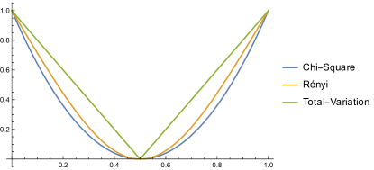
Figure 1: Plots for $\eta_{\chi^{2}}(\text{BSC}(\varepsilon))$, $\eta_{2}(\text{BSC}(\varepsilon))$ and $\eta_{\text{TV}}(\text{BSC}(\varepsilon))$.

References

• [1] R. Ahlswede and P. Gács, “Spreading of sets in product spaces and hypercontraction of the markov operator,” The annals of probability, pp. 925–939, 1976.
• [2] M. Raginsky, “Strong data processing inequalities and $\phi$-sobolev inequalities for discrete channels,” IEEE Transactions on Information Theory, vol. 62, no. 6, pp. 3355–3389, 2016.
• [3] Y. Polyanskiy and Y. Wu, “Strong data-processing inequalities for channels and bayesian networks,” in Convexity and Concentration.   Springer, 2017, pp. 211–249.
• [4] I. Csiszár, “Information-type measures of difference of probability distributions and indirect observation,” Studia Scientiarum Mathematicarum Hungarica, vol. 2, pp. 229–318, 1967. [Online]. Available: https://ci.nii.ac.jp/naid/10028997448/en/
• [5] F. Liese and I. Vajda, “On divergences and informations in statistics and information theory,” IEEE Trans. Inf. Theor., vol. 52, no. 10, pp. 4394–4412, 2006. [Online]. Available: http://dx.doi.org/10.1109/TIT.2006.881731
• [6] H. S. Witsenhausen, “On sequences of pairs of dependent random variables,” Siam Journal on Applied Mathematics, vol. 28, pp. 100–113, 1975. [Online]. Available: https://api.semanticscholar.org/CorpusID:123902515
• [7] V. Anantharam, A. Gohari, S. Kamath, and C. Nair, “On maximal correlation, hypercontractivity, and the data processing inequality studied by erkip and cover,” arXiv preprint arXiv:1304.6133, 2013.
• [8] J. E. Cohen, Y. Iwasa, G. Rautu, M. B. Ruskai, E. Seneta, and G. Zbaganu, “Relative entropy under mappings by stochastic matrices,” Linear algebra and its applications, vol. 179, pp. 211–235, 1993.
• [9] P. Del Moral, M. Ledoux, and L. Miclo, “On contraction properties of markov kernels,” Probability Theory and Related Fields, vol. 126, pp. 395–420, 01 2003.
• [10] T. Van Erven and P. Harremoës, “Rényi divergence and Kullback-Leibler divergence,” IEEE Transactions on Information Theory, vol. 60, no. 7, pp. 3797–3820, 2014.
• [11] A. R. Esposito and M. Mondelli, “Concentration without independence via information measures,” 2023.
• [12] L. Gross, “Logarithmic sobolev inequalities,” American Journal of Mathematics, vol. 97, no. 4, pp. 1061–1083, 1975. [Online]. Available: http://www.jstor.org/stable/2373688
• [13] A. R. Esposito, A. Vandenbroucque, and M. Gastpar, “Lower bounds on the Bayesian risk via information measure,” arXiv preprint arXiv:2303.12497, 2023, Journal of Machine Learning Research, accepted for publication.