Measuring Colloidomer Hydrodynamics with Holographic Video Microscopy

Abstract

In-line holographic video microscopy records a wealth of information about the microscopic structure and dynamics of colloidal materials. Powerful analytical techniques are available to retrieve that information when the colloidal particles are well-separated. Large assemblies of close-packed particles create holograms that are substantially more challenging to interpret. We demonstrate that Rayleigh-Sommerfeld back-propagation is useful for analyzing holograms of colloidomer chains, close-packed linear assemblies of micrometer-scale emulsion droplets. Colloidomers are fully flexible chains and undergo three-dimensional configurational changes under the combined influence of random thermal forces and hydrodynamic forces. We demonstrate the ability of holographic reconstruction to track these changes as colloidomers sediment through water in a horizontal slit pore. Comparing holographically measured configurational trajectories with predictions of hydrodynamic models both validates the analytical technique for this valuable class of self-organizing materials and also provides insights into the influence of geometric confinement on colloidomer hydrodynamics.

I Introduction

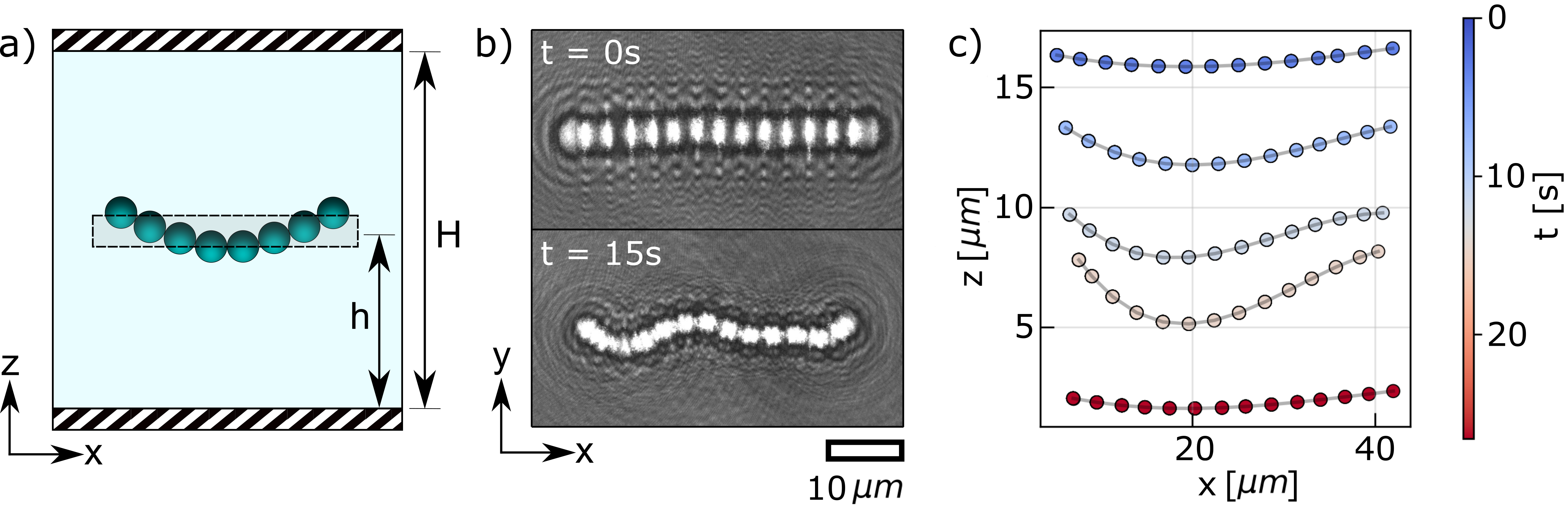
Figure 1: (a) Schematic view of a colloidomer’s confined sedimentation. A chain of droplets is suspended in a layer of water between two horizontal glass surfaces separated by height $H$. The colloidomer is lifted along the vertical $\hat{z}$ axis and stretched to its full extent along $\hat{x}$ by a pair of holographic optical tweezers. The traps then are extinguished, allowing the colloidomer to sediment freely. The chain bends and coils as it settles, and therefore is increasingly distorted relative to the ideal rod-like structure, shown at height $h$. (b) Holographic image of a model 14-droplet chain at two different times during its descent. (c) Trajectory of the chain from (b) obtained by analyzing holograms with Rayleigh-Sommerfeld backpropagation. Each point represents the three-dimensional position of one droplet, projected into the $x$-$z$ plane, and is colored by time. Hydrodynamic coupling to the lower wall suppresses curvature at late times.

The conformational dynamics of a confined polymer is strongly influenced by interactions with neighbors and hydrodynamic coupling to bounding surfaces. Such systems typically are studied through numerical simulation because the relevant length and time scales are not experimentally accessible. This situation recently has changed with the introduction of micrometer-scale colloidal analogs for molecular polymers. These include chains of colloidal spheres [1, 2] and emulsion droplets [3, 4, 5], linked by complementary DNA or nanoparticle bridges. These model soft-matter systems, known as colloidomers, behave in much the same way as conventional polymers with the advantage that they can be observed directly through optical microscopy. Experimental studies of colloidomer dynamics not only offer insights into the microscopic mechanisms of polymer physics, but also clarify how colloidomers can be induced to self-organize into hierarchical structures with practical applications [6].

The challenge in all such studies is to track the individual beads in a colloidal chain as they move relative to each other in three dimensions. Conventional microscopy cannot readily follow objects as they move out of the focal plane. Confocal microscopy solves this problem, but is too slow to track conformational changes. Lorenz-Mie analysis of holographic microscopy data addresses both of these issues [7], but is impractical for complex assemblies of particles [8], especially if their configuration changes over time. Here, we introduce a general method based on holographic video microscopy to measure the three-dimensional conformational trajectory of a colloidomer chain. We demonstrate this technique with an experimental study of fully flexible colloidomer chains sedimenting through a viscous fluid between two parallel hard walls. In addition to validating the technique, these measurements reveal the influence of hydrodynamic coupling on the dynamics of a flexible chain in quantitative agreement with hydrodynamic models.

Our system is shown schematically in Fig. 1(a). Colloidomer chains are assembled from monodisperse emulsion droplets composed of silicone oil stabilized with lipid surfactant. The population of droplets has a mean radius of $a_{p}=$1.58\pm 0.04\text{\,}\mathrm{\SIUnitSymbolMicro m}$$, as determined by Total Holographic Characterization (xSight, Spheryx) [7]. Droplets are linked into colloidomers using gold nanoparticles to act as bridges and are dispersed in a layer of water between two horizontal glass surfaces that are separated by $H\approx$24\text{\,}\mathrm{\SIUnitSymbolMicro m}$$. Links between droplets can flow freely across the droplets’ surfaces. Colloidomers therefore behave like freely jointed chains [4]. The sealed sample is mounted on the stage of an in-line holographic video microscope that is outfitted with holographic optical traps [9, 10]. Details of the colloidomers’ synthesis and characterization are provided in Appendix A.

Holograms of colloidomers, such as the examples in Fig. 1(b), are analyzed with Rayleigh-Sommerfeld back-propagation [11] to obtain the three-dimensional position of each droplet in the chain. These coordinates are then linked into the three-dimensional configuration of the chain at each recorded time step in its sedimentation, as shown in Fig. 1(c). Measurements on chains of different lengths reveal trends in sedimentation rate and curvature that can be compared with predictions based on models for the forces acting on the chain.

Previous studies [12, 2, 13] have noted that hydrodynamic coupling among the beads in a sedimenting chain reduces the viscous drag on beads near the center relative to those at the ends. As a consequence, the central beads tend to sediment faster, causing an initially linear chain to bend into a hairpin. The representative data in Fig. 1(c) illustrate how confinement by rigid walls suppresses the development of curvature, both at the beginning of the trajectory and also at the end. Measuring the dynamics of sedimenting colloidomers allows us to quantify the chains’ coupling to the walls and thus to test idealized models for bead-chain hydrodynamics.

II Tracking sedimenting chains with Rayleigh-Sommerfeld Backpropagation

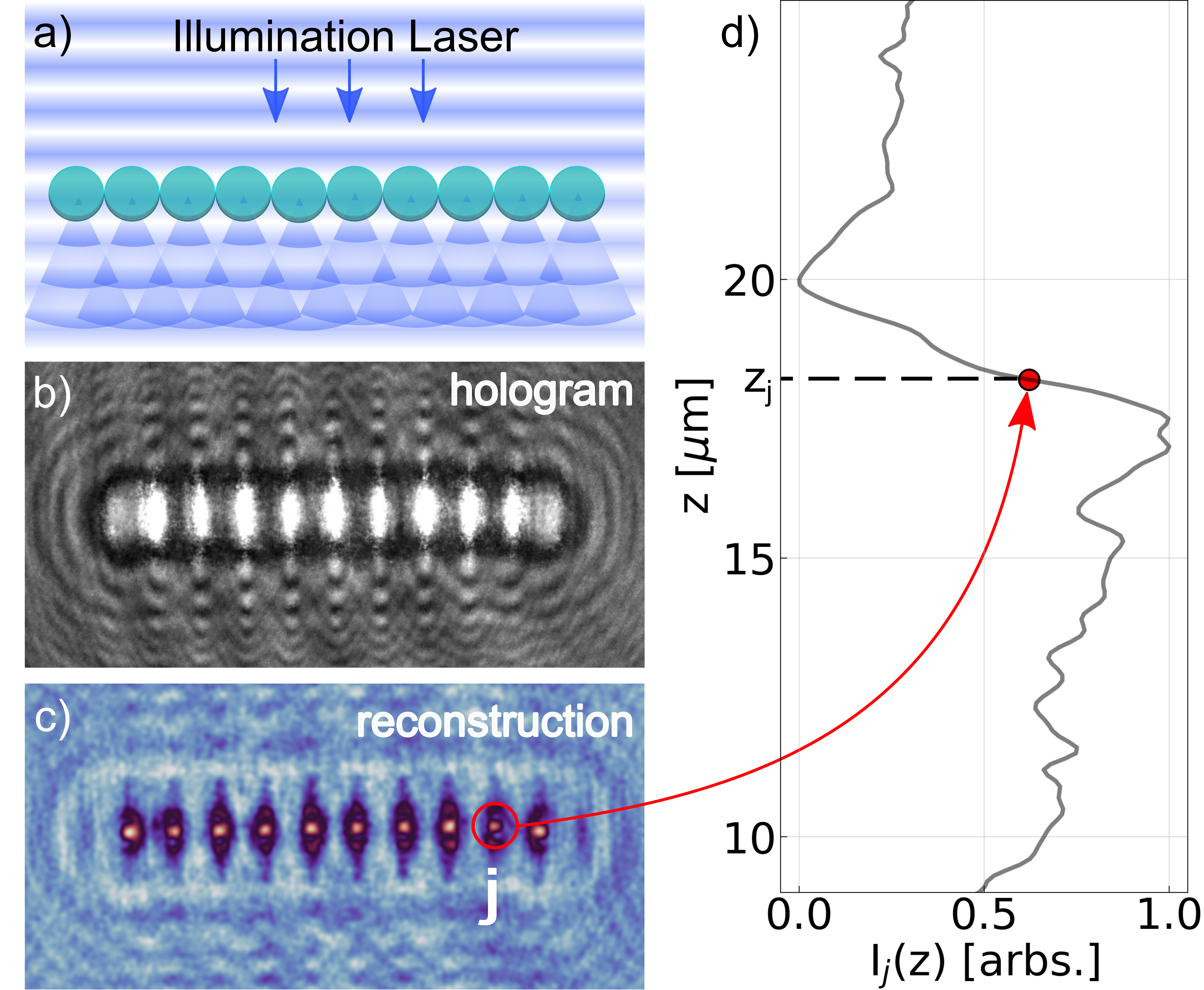
Figure 2: Holographic recording and reconstruction of a colloidomer’s three-dimensional configuration. (a) A chain of droplets is illuminated with a collimated laser beam. Interference between the scattered and incident light creates an intensity pattern that is magnified by a microscope and recorded with a video camera. (b) Hologram of a 10-droplet colloidomer stretched to its full extent with holographic optical tweezers. (c) Rayleigh-Sommerfeld reconstruction of the scattered intensity, $I_{R}(\boldsymbol{r},z)$, in the plane $z=$18\text{\,}\mathrm{\SIUnitSymbolMicro m}$$ above the microscope’s focal plane. (d) Axial dependence of the reconstructed intensity, $I_{j}(z)=I_{R}(\boldsymbol{r}_{j},z)$, at the in-plane position, $\boldsymbol{r}_{j}$, of one of the ten droplets. The inflection point is identified with the droplet’s axial position, $z_{j}(t)$, at time $t$. Similar reconstructions are performed for each droplet in the chain.

Figure 2 illustrates the measurement technique. The three-dimensional configuration of a colloidomer is recorded through in-line holographic video microscopy [14, 9]. As shown schematically in Fig. 2(a), the sample is illuminated with a collimated laser beam. Light scattered by the droplets interferes with the rest of the beam in the focal plane of a microscope. The intensity of the magnified interference pattern is then recorded with a standard video camera, as shown in Fig. 2(b). Each such video image is a hologram of the colloidomer and encodes information about each droplet’s size, refractive index and three-dimensional position [9]. Standard methods [7] to extract this information are confounded by the strongly overlapping scattering patterns from neighboring droplets. Rather than attempting to model such complex light-scattering patterns [15], we instead localize the individual droplets by numerically refocusing the hologram.

Given an estimate for the field scattered by a colloidomer into the focal plane, $E_{s}(\boldsymbol{r},0)$, we can numerically reconstruct the scattered field at height $z$ above the focal plane with the Rayleigh-Sommerfeld diffraction integral [16, 9, 17]:

$$E_{s}(\boldsymbol{r},z)=\int\tilde{E}_{s}(\boldsymbol{q},0)\,H(\boldsymbol{q},-z)\,e^{i\boldsymbol{q}\cdot\boldsymbol{r}}\,d^{2}q,$$ (1a)

where

$$\tilde{E}_{s}(\boldsymbol{q},0)=\int E_{s}(\boldsymbol{r},0)\,e^{-i\boldsymbol{q}\cdot\boldsymbol{r}}\,d^{2}r,$$ (1b)

and where

$$H(\boldsymbol{q},-z)=e^{iz(k^{2}-q^{2})^{\frac{1}{2}}}$$ (1c)

is the Fourier transform of the Rayleigh-Sommerfeld propagator [16]. The associated estimate for the scattered light’s intensity at height $$z$$ is

$$I_{s}(\boldsymbol{r},z)=\left|E_{s}(\boldsymbol{r},z)\right|^{2}.$$ (1d)

The intensity distribution recorded by the camera can be modeled as the superposition of the electric field due to the incident plane wave, $\boldsymbol{E}_{0}(\boldsymbol{r})$, and the scattered field in the focal plane, $\boldsymbol{E}_{s}(\boldsymbol{r},0)$ [9, 11]:

$$I(\boldsymbol{r},0) =\left|\boldsymbol{E}_{0}(\boldsymbol{r})+\boldsymbol{E}_{s}(\boldsymbol{r},0)\right|^{2}$$ (2a)

$$\approx I_{0}(\boldsymbol{r})+2\boldsymbol{E}_{0}^{\ast}(\boldsymbol{r})\cdot\boldsymbol{E}_{s}(\boldsymbol{r},0),$$ (2b)

where $I_{0}(\boldsymbol{r})=\left|\boldsymbol{E}_{0}(\boldsymbol{r})\right|^{2}$ is the intensity of the illumination in the absence of scatterers and where we assume that the intensity of the scattered wave is small enough compared with the other terms to be omitted. If, furthermore, the scatterer is far enough from the focal plane that polarization rotations can be neglected, the normalized hologram,

$$b(\boldsymbol{r})\equiv\frac{I(\boldsymbol{r},0)}{I_{0}(\boldsymbol{r})}-1,$$ (3a)

is related to the scattered field in the focal plane by

$$b(\boldsymbol{r})\approx\frac{E_{s}(\boldsymbol{r},0)}{E_{0}^{\ast}(\boldsymbol{r})}+\frac{E_{s}^{\ast}(\boldsymbol{r},0)}{E_{0}(\boldsymbol{r})}.$$ (3b)

This expression can be further simplified by modeling the collimated illumination as a plane wave aligned with the imaging plane so that $E_{0}^{\ast}(\boldsymbol{r})=E_{0}(\boldsymbol{r})=E_{0}$ [18].

Equation (3) shows that the normalized hologram records a superposition of the field scattered by the colloidomer and also a fictive field propagating in the opposite direction, which corresponds to the colloidomer’s mirror image in the focal plane. The associated twin image can be suppressed numerically [19, 20, 11] at the cost of additional computational complexity. If the colloidomer is far enough from the focal plane, however, perturbations due to the twin image are weak enough to ignore without further processing [11]. In that case, the scattered intensity, $I_{R}(\boldsymbol{r},z)$, at height $z$ above the focal plane can be reconstructed numerically from a measured hologram by substituting $b(\boldsymbol{r})$ for $E_{s}(\boldsymbol{r},0)$ in Eq. (1).

The image in Fig. 2(c) shows an estimate for the scattered intensity, $I_{R}(\boldsymbol{r},z)$, obtained from the hologram in Fig. 2(b) in the plane $z=$18\text{\,}\mathrm{\SIUnitSymbolMicro m}$$. Because this colloidomer has been stretched into a straight line by optical tweezers, all of the droplets come into sharpest focus in the same plane and appear in the reconstructed image as an array of small bright spots. Interestingly, these intensity maxima are offset from the brightest regions in the original hologram, which illustrates the diffractive nature of the image-formation process.

A quantitative estimate for a droplet’s three-dimensional position starts with an estimate for its in-plane position, $\boldsymbol{r}_{p}$, which might be obtained manually. The axial position, $z_{p}$, is then estimated by seeking the point of inflection in the numerically reconstructed axial intensity profile [9] along $\boldsymbol{r}_{p}$, as shown in Fig. 2(d). The image is then refocused to $z_{p}$ and the estimate for $\boldsymbol{r}_{p}$ is refined using standard particle-tracking algorithms [21]. Finally, $z_{p}$ is refined using the improved estimate for $\boldsymbol{r}_{p}$. Numerical uncertainties in the fit values suggest that this protocol achieves a precision of $\Delta r_{p}=$0.1\text{\,}\mathrm{p}\mathrm{i}\mathrm{x}\mathrm{e}\mathrm{l}$=$5\text{\,}\mathrm{nm}$$ for the droplet’s in-plane position and $\Delta z_{p}=$1\text{\,}\mathrm{p}\mathrm{i}\mathrm{x}\mathrm{e}\mathrm{l}$=$48\text{\,}\mathrm{nm}$$ along the axial direction.

The same procedure can be performed for each droplet in a chain and yields a snapshot of the colloidomer’s instantaneous configuration. The mean separation between droplet centers,

$$\Delta r=\frac{1}{N-1}\sum_{j=1}^{N-1}\left|\boldsymbol{r}_{j}(t)-\boldsymbol{r}_{j+1}(t)\right|,$$ (4)

should be equal to the diameter of a single droplet. The data in Fig. 1 yield $\Delta r/2=$1.5\pm 0.1\text{\,}\mathrm{\SIUnitSymbolMicro m}$$, which is consistent with the holographically measured radius, $a_{p}=$1.58\pm 0.04\text{\,}\mathrm{\SIUnitSymbolMicro m}$$, for the population of emulsion droplets used to assemble the chain. This agreement helps to validate the tracking technique.

The data in Fig. 1(c) show the projection of a colloidomer’s three-dimensional configuration onto the $x$-$z$ plane as it freely sediments within its sample cell. Such configurational trajectories can be compared with predictions of hydrodynamic models both to validate the tracking technique and also to cast new light on the influence of confinement on colloidomer dynamics.

III Sedimentation of confined chains of beads

III.1 Sedimentation of a rigid chain

The drag force experienced by an isolated sphere of radius $a_{p}$ moving with velocity $\boldsymbol{v}$ through a viscous fluid is given by [22],

$$\boldsymbol{F}(\boldsymbol{v})=-\gamma_{0}\,\boldsymbol{v},\quad\text{where}$$ (5a)

$$\gamma_{0}=6\pi\eta\,a_{p}$$ (5b)

is the Stokes drag coefficient in a fluid of viscosity $\eta$. A fully extended chain of spheres sedimenting perpendicularly to its axis can be modeled as a long ellipsoid, for which the drag coefficient is [22]

$$\gamma_{\infty}=\frac{8\pi\eta\,a}{\ln\left(2\frac{a}{b}\right)+\frac{1}{2}},$$ (6)

where $a$ and $b$ are the semi-major and semi-minor axes, respectively. Combining Eqs. (5b) and (6) suggests that the drag coefficient for an extended chain of $N$ spheres is approximately

$$\gamma_{N}=\frac{4}{3}\left(\frac{N}{\ln{2N}+\frac{1}{2}}\right)\gamma_{0}$$ (7)

in the limit $N\gg 1$. The denominator of Eq. (7) implicitly incorporates hydrodynamic coupling among the spheres, albeit without allowing the spheres to rearrange themselves.

III.2 Confinement by a slit pore

Hydrodynamic coupling to bounding surfaces enhances the drag on a moving object. For a sphere moving perpendicularly to a rigid wall, Faxén shows that [23, 22]

$$\gamma(h)\approx\gamma_{0}\left(1-\frac{9}{8}\frac{a_{p}}{h}\right)^{-1},$$ (8)

where $h$ is the distance from the center of the sphere to the wall. The analogous result for a horizontal chain of spheres at height $h$ above a horizontal wall is [24]

$$\gamma_{N}(h)=\gamma_{N}\left(1-\frac{9}{8}\frac{a_{p}}{h}\frac{\gamma_{N}}{\gamma_{0}}\right)^{-1}.$$ (9)

Adding a second parallel wall at distance $H$ from the first, as shown in Fig. 1(a), disproportionately increases the complexity of the drag calculation [25]. If $H\gg a_{p}$, however, we may invoke Oseen’s linear superposition approximation [26],

$$\gamma_{N}(h,H)\approx\gamma_{N}(h)+\gamma_{N}(H-h)-\gamma_{N}.$$ (10)

With these simplifying approximations, a horizontally extended colloidomer sedimenting through a viscous fluid in the space between two horizontal plane walls should fall with a speed that depends on its height in the channel,

$$v_{p}(h)=\frac{N}{\gamma_{N}(h,H)}\,\Delta m_{p}g,\quad\text{where}$$ (11a)

$$\Delta m_{p}=\frac{4}{3}\pi\,a_{p}^{3}\,\Delta\rho_{p}$$ (11b)

is the buoyant mass of a single droplet given its buoyant mass density, $\Delta\rho_{p}$, and where $g=$9.81\text{\,}\mathrm{m}\text{\,}{\mathrm{s}}^{-2}$$ is the acceleration due to gravity.

IV Results

IV.1 Measured sedimentation of confined colloidomers

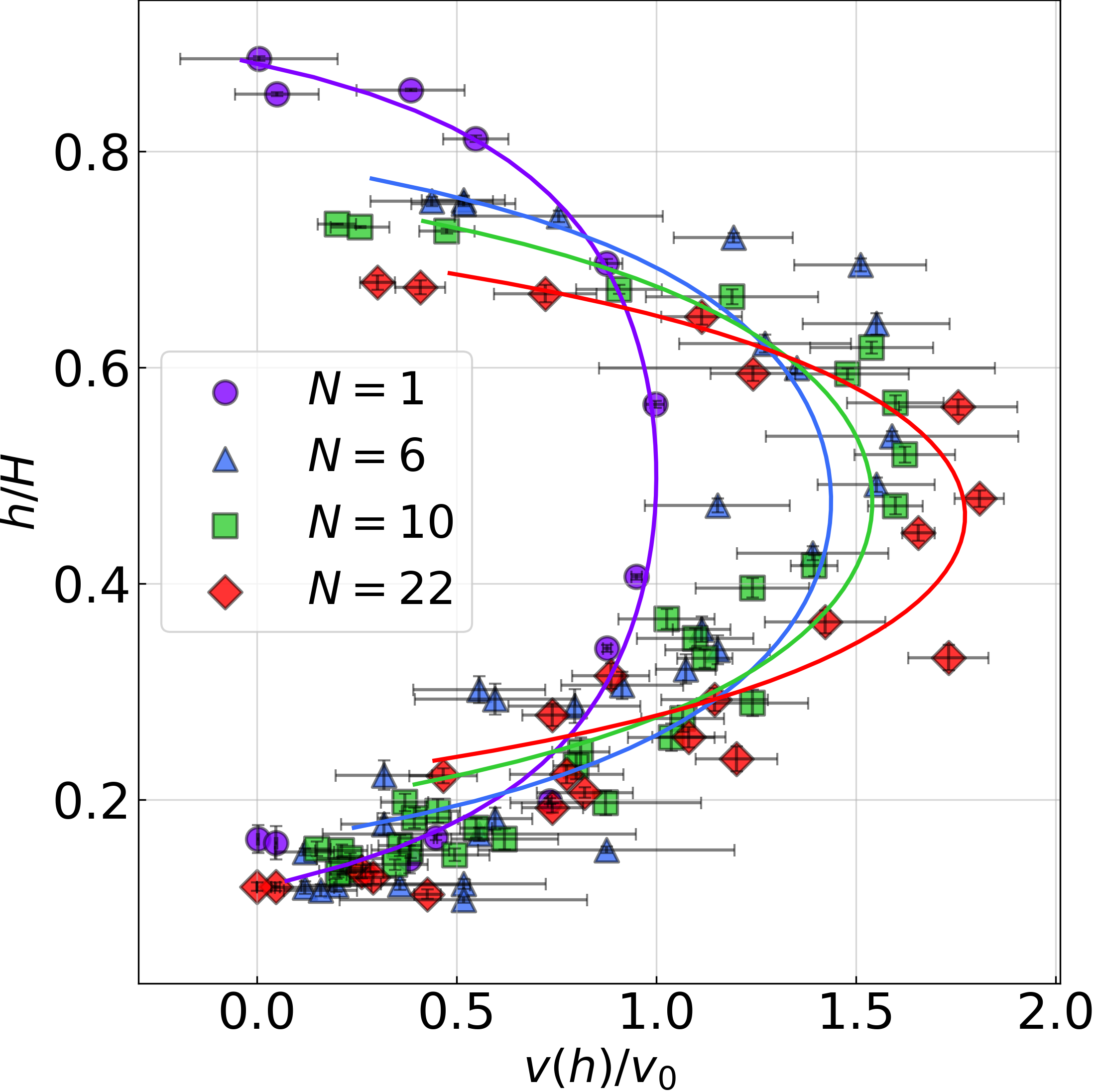
Figure 3: Velocity profiles of sedimenting colloidomers of chain lengths $N=6$, 10 and 22. Monomer data ($N=1$) are fit to Eq. (11) with $\gamma_{N}=\gamma_{0}$ . The fit yields the droplet’s buoyant density, $\Delta\rho_{p}=$166\pm 7.\text{\,}\mathrm{kg}\text{\,}{\mathrm{m}}^{-3}$$, and the wall separation, $H$. Colloidomer data are fit to Eq. (11) using the same value for the droplet density, leaving only $H$ as an adjustable parameter.

Figure 3 presents measurements of colloidomers’ sedimentation speed, $v(h)$, as a function of height in the channel, $h$, and the number of droplets in the chain, $N$. A measurement is initiated by trapping the two ends of a colloidomer with a pair of holographic optical tweezers, stretching the chain to its maximum extension, lifting it to a height $h$ above the sample chamber’s lower wall, and then extinguishing the traps to let the chain sediment freely. The optical traps are powered by a fiber laser (IPG Photonics, YLR-LP-SF) operating at a vacuum wavelength of $1064\text{\,}\mathrm{nm}$. The light is formed into programmable optical traps by imprinting it with computer-generated holograms using a liquid-crystal spatial light modulator (Holoeye PLUTO) [27, 28, 29, 10]. The holograms are projected through the microscope’s objective lens using the standard holographic optical trapping technique [30, 31] and are controlled using the pyfab interface [32].

In-line holographic imaging is performed with a $3\text{\,}\mathrm{mW}$ collimated beam provided by a fiber-coupled diode laser (Coherent Cube) operating at a vacuum wavelength of $\lambda=$447\text{\,}\mathrm{nm}$$. The beam’s $3\text{\,}\mathrm{mm}$ waist barely overfills the input pupil of the microscope’s objective lens (Nikon Plan Apo, 100×, numerical aperture 1.4, oil immersion). A small proportion of the incident light is scattered by the chain of droplets and interferes with the remainder of the beam in the focal plane of the objective lens. The magnified interference pattern is relayed to a monochrome video camera (FLIR Flea3 USB 3.0) that records its intensity every $\Delta t=$66\text{\,}\mathrm{ms}$$. The exposure time of $100\text{\,}\mathrm{\SIUnitSymbolMicro s}$ is fast enough to avoid distortions due to motion blurring [33].

Each holographic snapshot in the video stream is analyzed with the methods of Sec. II. A colloidomer’s height, $h(t)$, at time $t$ is computed as the average of the axial positions of its constituent droplets. The uncertainty in the height consists of the standard deviation of the droplets’ axial positions in quadrature with the numerical error in the single-droplet measurements. The colloidomer’s sedimentation speed is computed as the change in height during the camera’s frame interval, $\Delta t$. All speeds are scaled by the sedimentation speed for a single sphere at the midplane,

$$v_{0}=\frac{\Delta m_{p}g}{\gamma_{0}}\left(1-\frac{9}{2}\frac{a_{p}}{H}\right),$$ (12)

which is found to be $v_{0}=$0.79(0.02)\text{\,}\mathrm{\SIUnitSymbolMicro m}\text{\,}{\mathrm{s}}^{-1}$$ by fitting to the unscaled data for $N=1$. Figure 3 presents the scaled results for the single droplet.

The single-droplet fit yields the buoyant density of the silicone oil mixture, $\Delta\rho_{p}=$166\pm 7.\text{\,}\mathrm{kg}\text{\,}{\mathrm{m}}^{-3}$$, and the height of the channel, $H$. The former is consistent with independent measurements using a density meter (DMA 4500 M, Anton Paar) and is treated as a fixed parameter when analyzing the data for colloidomers. Because different sample cells have slightly different heights, $H\approx$25\text{\,}\mathrm{\SIUnitSymbolMicro m}$$ is treated as an adjustable parameter for each experiment and is resolved to within $100\text{\,}\mathrm{nm}$.

The solid curves in Fig 3 are single-parameter fits to Eq. (11) for chains of length $N=6$, 10 and 22. Predictions of the rigid-chain model agree well with the measured sedimentation profiles of colloidomers despite the colloidomers’ flexibility.

Colloidomers sediment more slowly near walls than individual spheres because of the length-dependent enhancement to hydrodynamic coupling described by Eq. (9). This effect is stronger for longer chains. Conversely, colloidomers sediment more rapidly than individual spheres near the middle of the channel where wall-induced drag has less influence than the drag reduction afforded by coupling to neighboring droplets. The crossover between these two effects is modeled by the length-dependent denominator in Eq. (7). None of these comparisons, however, take account of the curvature that develops as colloidomers sediment.

IV.2 Curvature of confined sedimenting colloidomers

Hydrodynamic coupling reduces the drag on droplets near the center of the chain relative to those at the ends. The central droplets therefore should sediment faster, causing the chain to bend, and eventually to adopt a hairpin configuration [12, 2]. The tendency for the center of a flexible chain to sediment fastest is evident in the early stages of the trajectory plotted in Fig. 1(c).

Hydrodynamic coupling to the upper wall complicates this process because the associated contribution to the drag tends to be greater for spheres near the center of the chain, which have more neighbors. The additional drag tends to suppress the emergence of curvature relative to a free chain. Once curvature develops, however, this contribution to the wall-associated drag will most strongly affect the droplets that remain closest to the wall, accelerating the evolution of curvature. Depending on chain length and its initial distance from the upper wall, this competition could favor the development of negative curvature, with the end droplets initially falling faster than the central droplets [34].

We avoid this complication by releasing the chains away from the upper wall thereby weakening that wall’s influence on the chains’ dynamics and focusing attention on the lower wall’s influence. As indicated in Fig. 1(c), colloidomers are stretched to their full extent with optical tweezers, lifted to height $h=$0.7$H$ in the channel and then released to sediment freely. Figure 4 shows how a colloidomer’s curvature evolves as it sediments. The instantaneous curvature at arc length $s$ along the time-evolving three-dimensional conformation, $\boldsymbol{r}(s,t)$, may be computed as

$$\kappa(s,t)=\frac{\left|\boldsymbol{r}^{\prime}\times\boldsymbol{r}^{\prime\prime}\right|}{\left|\boldsymbol{r}^{\prime}\right|^{3}},$$ (13)

where primes denote derivatives with respect to $s$. Equation (13) can be approximated for the discrete vertices of a colloidomer by the three-point Menger curvature. The discrete points in Fig. 4(a) report the maximum curvature, $\kappa(h)=\max\{\kappa(s,h)\}$, for colloidomers of length $N=10$, 14 and 22, where $h=h(t)$ is the colloidomer’s mean height in the channel at time $t$. The shaded regions indicate the range of curvature values between the mean curvature and the maximum.

Introducing curvature into a colloidomer involves moving droplets longitudinally along the chain to conserve the chain’s length. The associated contribution to the drag is proportional to the total amount of longitudinal displacement and therefore is proportional to the length of the chain. Scaling the curvature by the chain length therefore yields a dimensionless curvature that should increase linearly with time as the chain sediments [2]. The data collapse in Fig. 4(b) is consistent with this interpretation under conditions where the chains are near the channel’s midplane and confinement effects are weak.

Hydrodynamically mediated curvature is augmented by Brownian coiling [4], whose influence can be seen in Fig. 1(b). The curvature due to coiling can exceed that for hydrodynamic bending in a long chain that sediments slowly. The curvature plotted in Fig. 4 therefore becomes increasingly noisy at later times, especially for the longest chain with $N=22$.

As the chain sediments below the midplane of the channel, its hydrodynamic coupling to the lower wall increases. This tends to reduce its hydrodynamically induced curvature even before the bottom-most droplets touch down. Once the chain makes contact, the vertical component of its curvature is mechanically suppressed, leaving only the in-plane curvature due to coiling.

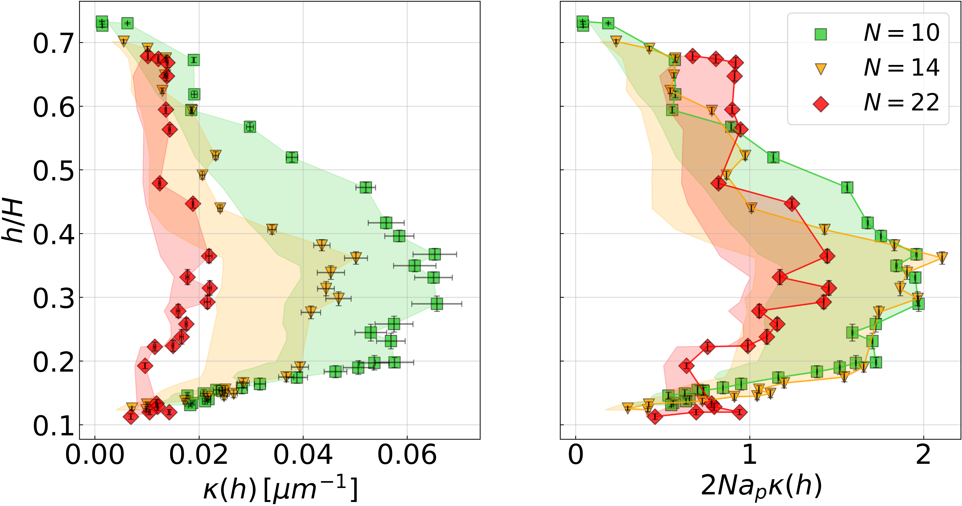
Figure 4: (a) The maximum three-point curvature of a colloidomer chain, $\kappa(h)$, as a function of the colloidomer’s mean height in the channel. Data are shown for $N=10$ (green squares), $N=14$ (gold inverted triangles), and $N=22$ (red diamonds). Shaded areas show the range between mean and maximum values. (b) Scaling the curvature by the chain length effectively collapses the three data sets.

V Discussion

Holographic microscopy is a powerful tool for measuring the three-dimensional trajectories of micrometer-scale objects [9, 7]. Taking a targeted approach to Rayleigh-Sommerfeld reconstruction extends these capabilities to systems, such as colloidomers, that consist of close-packed particles. Measurements of colloidomer sedimentation in a slit pore validate the technique by yielding results for chains’ trajectories that are consistent with hydrodynamic models.

Appendix A Colloidomer Synthesis

Our emulsion droplets are created from a 1:1:1 mixture by volume fraction of three types of silane monomers: (a) dimethyldiethoxysilane (Sigma-Aldrich), commonly known as DMDES, (b) (3,3,3-trifluoropropyl) methyldimethoxysilane (Gelest), and (c) 3-glycidoxypropylmethyldiethoxysilane (Gelest). Droplets are condensed out of an aqueous monomer solution by ammonia-catalyzed hydrolysis and condensation following the procedure described in Ref. [35]. Specifically, $175\text{\,}\mathrm{\SIUnitSymbolMicro L}$ of monomer is dissolved in $3.115\text{\,}\mathrm{mL}$ of deionized water by vortexing. Droplet nucleation is initiated by adding $1\text{\,}\mathrm{\char 37\relax}\mathrm{v}\mathrm{/}\mathrm{v}$ of $27\text{\,}\mathrm{\char 37\relax}$ ammonium hydroxide solution (Sigma-Aldrich). Droplet growth is stopped after 6 hours by washing the sample with $1\text{\,}\mathrm{mM}$ sodium dodecyl sulfate solution (SDS, Sigma-Aldrich). The sample is centrifuged and resuspended with $1\text{\,}\mathrm{mM}$ SDS solution three times. The completed emulsion is stored in $5\text{\,}\mathrm{mM}$ SDS.

The droplets are stabilized with lipid surfactants. Lipid labeling is achieved by diluting $10\text{\,}\mathrm{\SIUnitSymbolMicro L}$ of packed droplets with $190\text{\,}\mathrm{\SIUnitSymbolMicro L}$ of $5\text{\,}\mathrm{mM}$ SDS solution containing $1\text{\,}\mathrm{\SIUnitSymbolMicro L}$ DSPE-PEG-SH thiol-terminated lipid (Avanti Polar Lipids, MW 2000). The mixture is kept on a rotary mixer overnight. Excess lipid is washed off by centrifuging, and replacing the supernatant layer with $1\text{\,}\mathrm{mM}$ SDS each time.

Droplets are assembled into linear chains using methods described in Refs. [36, 35, 37]. The emulsion droplets are first concentrated by centrifugation before being redispersed in a commercial ferrofluid (EMG 707, Ferrotec) along with $1\text{\,}\mathrm{mM}$ Tris-EDTA (Thermo Fischer Scientific) at pH 8 and $30\text{\,}\mathrm{nm}$-diameter gold nanoparticles (BBI Solutions, EMGC30) at a concentration of ${10}^{11}\text{\,}{\mathrm{mL}}^{-1}$. This mixture is imbibed into a rectangular capillary tube (VitroCom) by capillary action and is subjected to an external magnetic field of roughly $1\text{\,}\mathrm{T}$ aligned with the capillary’s long axis that is applied with a pair of neodymium rare-earth magnets. The emulsion droplets act as diamagnetic bubbles in the ferrofluid and are organized into chains aligned with the field by induced-dipole interactions.

Individual droplets become decorated with gold nanoparticles that bind irreversibly to the lipids’ terminal thiol groups. Once bound, the gold nanoparticles diffuse across the droplets’ fluid surfaces until they reach the contact region between neighboring droplets. There, they form bridges between the droplets, binding the field-induced lines of droplets into permanent colloidomer chains. The droplets remain in a fluid state so that the inter-droplet bonds are fully flexible. Hematite nanoparticles from the ferrofluid are prevented from binding to the thiol groups through the addition of EDTA.

Stable colloidomer chains form after roughly two hours at room temperature, after which they are washed out of the capillary into $100\text{\,}\mathrm{\SIUnitSymbolMicro L}$ of $0.5\text{\,}\mathrm{\char 37\relax}\mathrm{v}\mathrm{/}\mathrm{v}$ Pluronic F-108 solution (Sigma-Aldrich). Excess ferrofluid is pipetted off the top with the help of a bar magnet. The remaining sample is pipetted between a glass microscope slide and a glass #1.5 coverslip (Globe Scientific), and sealed using UV-cured adhesive (LOON, UV Clear Fly Finish).

References

- Byrom et al. [2014] J. Byrom, P. Han, M. Savory, and S. L. Biswal, Directing assembly of DNA-coated colloids with magnetic fields to generate rigid, semiflexible, and flexible chains, Langmuir 30, 9045 (2014).
- Cunha et al. [2022] L. H. Cunha, J. Zhao, F. C. MacKintosh, and S. L. Biswal, Settling dynamics of Brownian chains in viscous fluids, Phys. Rev. Fluids 7, 034303 (2022).
- Feng et al. [2013] L. Feng, L.-L. Pontani, R. Dreyfus, P. Chaikin, and J. Brujic, Specificity, flexibility and valence of DNA bonds guide emulsion architecture, Soft Matter 9 (2013).
- McMullen et al. [2018] A. McMullen, M. Holmes-Cerfon, F. Sciortino, A. Y. Grosberg, and J. Brujic, Freely jointed polymers made of droplets, Phys. Rev. Lett. 121, 138002 (2018).
- McMullen et al. [2022] A. McMullen, M. Muñoz Basagoiti, Z. Zeravcic, and J. Brujic, Self-assembly of emulsion droplets through programmable folding, Nature 610, 502–506 (2022).
- Coulais et al. [2018] C. Coulais, A. Sabbadini, F. Vink, and M. van Hecke, Multi-step self-guided pathways for shape-changing metamaterials, Nature 561, 512 (2018).
- Lee et al. [2007] S.-H. Lee, Y. Roichman, G.-R. Yi, S.-H. Kim, S.-M. Yang, A. Van Blaaderen, P. Van Oostrum, and D. G. Grier, Characterizing and tracking single colloidal particles with video holographic microscopy, Opt. Express 15, 18275 (2007).
- Fung et al. [2012] J. Fung, R. W. Perry, T. G. Dimiduk, and V. N. Manoharan, Imaging multiple colloidal particles by fitting electromagnetic scattering solutions to digital holograms, J. Quant. Spectrosc. Radiat. Transf. 113, 2482 (2012).
- Lee and Grier [2007] S.-H. Lee and D. G. Grier, Holographic microscopy of holographically trapped three-dimensional structures, Opt. Express 15, 1505 (2007).
- O’Brien and Grier [2019] M. J. O’Brien and D. G. Grier, Above and beyond: Holographic tracking of axial displacements in holographic optical tweezers, Opt. Express 27, 25375 (2019).
- Dixon et al. [2011a] L. Dixon, F. C. Cheong, and D. G. Grier, Holographic deconvolution microscopy for high-resolution particle tracking, Opt. Express 19, 16410 (2011a).
- Li et al. [2013] L. Li, H. Manikantan, D. Saintillan, and S. E. Spagnolie, The sedimentation of flexible filaments, J. Fluid Mech. 735, 705–736 (2013).
- Shashank et al. [2023] H. Shashank, Y. Melikhov, and M. L. Ekiel-Jeżewska, Dynamics of ball chains and highly elastic fibres settling under gravity in a viscous fluid, Soft Matter 19, 4829 (2023).
- Sheng et al. [2006] J. Sheng, E. Malkiel, and J. Katz, Digital holographic microscope for measuring three-dimensional particle distributions and motions, Appl. Opt. 45, 3893 (2006).
- Martin et al. [2022] C. Martin, L. E. Altman, S. Rawat, A. Wang, D. G. Grier, and V. N. Manoharan, In-line holographic microscopy with model-based analysis, Nat. Rev. Methods Primers 2, 83 (2022).
- Goodman [2005] J. W. Goodman, Introduction to Fourier Optics, 3rd ed. (McGraw-Hill, New York, 2005).
- Cheong et al. [2010] F. C. Cheong, B. J. Krishnatreya, and D. G. Grier, Strategies for three-dimensional particle tracking with holographic video microscopy, Opt. Express 18, 13563 (2010).
- Moyses et al. [2013] H. W. Moyses, B. J. Krishnatreya, and D. G. Grier, Robustness of Lorenz-Mie microscopy against defects in illumination, Opt. Express 21, 5968 (2013).
- Latychevskaia and Fink [2007] T. Latychevskaia and H.-W. Fink, Solution to the twin image problem in holography, Phys. Rev. Lett. 98, 233901 (2007).
- Zhang et al. [2018] W. Zhang, L. Cao, D. J. Brady, H. Zhang, J. Cang, H. Zhang, and G. Jin, Twin-image-free holography: a compressive sensing approach, Phys. Rev. Lett. 121, 093902 (2018).
- Crocker and Grier [1996] J. C. Crocker and D. G. Grier, Methods of digital video microscopy for colloidal studies, J. Colloid Interf. Sci. 179, 298 (1996).
- Happel and Brenner [1991] J. Happel and H. Brenner, Low Reynolds Number Hydrodynamics (Kluwer, Dordrecht, 1991).
- Brenner [1962] H. Brenner, Effect of finite boundaries on the Stokes resistance of an arbitrary particle, J. Fluid Mech. 12, 35 (1962).
- Hadamard [1911] J. S. Hadamard, Mouvement permanent lent d’une sphère liquide et visqueuse dans un liquide visqueux, C. R. Acad. Sci. 152, 1735 (1911).
- Liron and Mochon [1976] N. Liron and S. Mochon, Stokes flow for a stokeslet between two parallel flat plates, J. Eng. Math. 10 (1976).
- Dufresne et al. [2000] E. R. Dufresne, D. Altman, and D. G. Grier, Brownian dynamics of a sphere between parallel walls, EPL 53, 264 (2000).
- Reicherter et al. [1999] M. Reicherter, T. Haist, E. U. Wagemann, and H. J. Tiziani, Optical particle trapping with computer-generated holograms written on a liquid-crystal display, Opt. Lett. 24, 608 (1999).
- Curtis et al. [2002] J. E. Curtis, B. A. Koss, and D. G. Grier, Dynamic holographic optical tweezers, Opt. Commun. 207, 169 (2002).
- Polin et al. [2005] M. Polin, K. Ladavac, S.-H. Lee, Y. Roichman, and D. G. Grier, Optimized holographic optical traps, Opt. Express 13, 5831–5845 (2005).
- Grier [2003] D. G. Grier, A revolution in optical manipulation, Nature 424, 810–816 (2003).
- Dufresne and Grier [1998] E. R. Dufresne and D. G. Grier, Optical tweezer arrays and optical substrates created with diffractive optical elements, Rev. Sci. Instrum. 69, 1974–1977 (1998).
- Grier et al. [2024] D. G. Grier, J. Sustiel, S. Zare, and N. Wittler, pyfab: Platform for holographic optical trapping, Zenodo 10.5281/zenodo.10719303 (2024).
- Dixon et al. [2011b] L. Dixon, F. C. Cheong, and D. G. Grier, Holographic particle-streak velocimetry, Opt. Express 19, 4393 (2011b).
- Perrin et al. [2019] H. Perrin, A. Eddi, S. Karpitschka, J. H. Snoeijer, and B. Andreotti, Peeling an elastic film from a soft viscoelastic adhesive: experiments and scaling laws, Soft Matter 15, 770 (2019).
- Elbers et al. [2015] N. A. Elbers, J. Jose, A. Imhof, and A. van Blaaderen, Bulk scale synthesis of monodisperse PDMS droplets above 3 m and their encapsulation by elastic shells, Chem. Mater. 27, 1709 (2015).
- Obey and Vincent [1994] T. M. Obey and B. Vincent, Novel Monodisperse “Silicone Oil”/Water Emulsions, J. Colloid Interf. Sci. 163, 454 (1994).
- McMullen et al. [2021] A. McMullen, S. Hilgenfeldt, and J. Brujic, DNA self-organization controls valence in programmable colloid design, PNAS 118, e2112604118 (2021).