First Passage Percolation with Queried Hints

Abstract

Solving optimization problems leads to elegant and practical solutions in a wide variety of real-world applications. In many of those real-world applications, some of the information required to specify the relevant optimization problem is noisy, uncertain, and expensive to obtain. In this work, we study how much of that information needs to be queried in order to obtain an approximately optimal solution to the relevant problem. In particular, we focus on the shortest path problem in graphs with dynamic edge costs. We adopt the first passage percolation model from probability theory wherein a graph $G^{\prime}$ is derived from a weighted base graph $G$ by multiplying each edge weight by an independently chosen random number in $[1,\rho]$. Mathematicians have studied this model extensively when $G$ is a $d$-dimensional grid graph, but the behavior of shortest paths in this model is still poorly understood in general graphs. We make progress in this direction for a class of graphs that resemble real-world road networks. Specifically, we prove that if $G$ has a constant continuous doubling dimension, then for a given $s-t$ pair, we only need to probe the weights on $((\rho\log n)/\epsilon)^{O(1)}$ edges in $G^{\prime}$ in order to obtain a $(1+\epsilon)$-approximation to the $s-t$ distance in $G^{\prime}$. We also generalize the result to a correlated setting and demonstrate experimentally that probing improves accuracy in estimating $s-t$ distances.

1 Introduction

Path search in dynamic systems such as traffic networks is a foundational problem in computer science. Dijkstra’s algorithm does not suffice for path search in large graphs, like continent-scale road networks. Work began on efficient path search in the early 2000s, with the development of reach (Gutman, 2004; Goldberg et al., 2006), contraction hierarchies (Geisberger et al., 2008), and more (Bast et al., 2006, 2007; Bauer and Delling, 2010; Goldberg and Harrelson, 2005; Hilger et al., 2009; ich Lauther, 2006; Sanders and Schultes, 2005). Theoretical justification for the efficiency of these methods came shortly after with the introduction of highway dimension (Abraham et al., 2010). These techniques have seen widespread adoption in routing engines.

Efficiency is not the only requirement for a useful path search engine. Users want customized routes that adapt to real-world conditions. In particular, path search engines need to find the shortest path subject to current real-world traffic and road-closure conditions. This requires designing a path search engine that can handle edge weight modifications. In the 2010s, customizable route planning (CRP) (Delling et al., 2011) was developed to handle changing edge weights.

All of these techniques involve redoing expensive preprocessing every time the graph changes. For instance, CRP starts with a partition of the input graph and precomputes shortcuts between boundary nodes of each cluster. When traffic conditions change, CRP needs to rebuild all shortcuts associated with clusters in which an edge weight changed. Traffic conditions generally change throughout the input road network, necessitating recomputation of almost all shortcuts.

One may wonder, though, when recomputation needs to be done. In particular, if the traffic conditions on a short surface street change, only routes with nearby origin and destination are likely to be affected, so no recomputation of shortcuts should be necessary. In this work, we show both theoretically and experimentally that this recomputation is indeed unnecessary for most edge weight changes. We show, under random traffic, only a small number of real traffic values need to be queried in order to obtain a good approximation to the origin-destination distance with traffic (Theorem 1.2).

1.1 Theoretical Result: Independent Models

We now briefly discuss our theoretical results, leaving formal definitions to Section 2. In both our theoretical and experimental results, we always use random noise to model traffic, though not always noise that is independent across all edges. In our theoretical results, the graph is always undirected, though in experiments the graphs are directed. We always start with a weighted graph (e.g. road network) $G$, with weights intuitively representing free-flow traffic values. To generate traffic, multiply each edge weight by a random number in $[1,\rho]$ to produce a graph $G^{\prime}$, representing a road network with traffic. Given an origin-destination pair $s-t$, our goal is to compute an $s-t$ path that is as short as possible within $G^{\prime}$ without actually querying many edges in $G^{\prime}$. This, in the application, would amount to computing an approximate traffic-aware shortest path without much real traffic information. Specifically, given a bound on the number of probes required, we can obtain a traffic-aware distance data structure from a no-traffic one when edge weights are independently chosen:

Theorem 1.1.

Suppose that Algorithm 1 probes at most $K_{0}$ edges and that, given an $\delta>0$ and a graph $G$, there exists a data structure $\mathcal{X}$ that takes $K_{1}$ time to initialize and is equipped with a method ApproxNoTrafficDistance($s,t,G$) that outputs a $(1+\delta)$-approximation to $d_{G}(s,t)$ in $K_{2}$ time. Then, given $\epsilon>0$, an $m$-edge graph $G$, a (traffic) weight distribution $\mathcal{D}$ in which edges are independent, and query access to a hidden graph $G^{\prime}$ as described previously, there exists a data structure $\mathcal{Y}$ that takes $\tilde{O}(m+K_{1})$ time to initialize and is equipped with a method ApproxTrafficDistance($s,t,\mathcal{D},G,G^{\prime}$) that computes a $(1+\epsilon)$-approximation to $d_{G^{\prime}}(s,t)$ with probability at least $1-1/m^{8}$ in $\tilde{O}(K_{0}^{2}K_{2})$ time.

We prove this result in Section A.1. As per (Abraham et al., 2010), $K_{1}=\tilde{O}(m)$ and $K_{2}=\text{polylog}(n)$ in practice. Therefore, if we can bound the number of probes $K_{0}$, then we obtain a data structure for traffic routing with polylogarithmic runtime per query. Thus, we focus on the problem of showing that few probes to $G^{\prime}$ are required to compute shortest paths in $G^{\prime}$. Doing this for arbitrary graphs $G^{\prime}$ is impossible, as in graphs $G^{\prime}$ with a large number of parallel edges, one has to query all of the parallel edges in order to find an approximately shortest $s-t$ path. However, this behavior is not realistic in practice, as it would require the existence of lots of potentially optimal disjoint paths between a given origin and destination. This is implausible in road networks, as most shortest paths use highways at some point and there are not many highways to choose from. This observation motivated the work of (Abraham et al., 2010) and led them to only consider the class of graphs that have what they called low highway dimension. Since we only care (and can) find approximately shortest paths, we can show results for a broader class of graphs – graphs with low continuous doubling dimension (cdd).

A graph has doubling dimension ${\alpha}$ if the ball of radius $2R$ around any vertex $v$ can be written as the union of balls of radius $R$ around a collection of at most $2^{\alpha}$ other vertices. This definition is motivated by what happens in $\mathbb{R}^{\alpha}$, as any ${\alpha}$-dimensional ball of radius $2R$ can be covered with at most $6^{\alpha}$ balls of radius $R$. Road networks are often assumed to have low doubling dimension (Abraham et al., 2006, 2016; Feldmann and Marx, 2018). For our purposes, we need a slightly stronger property: we need the the graph where each edge is chopped up into infinitesimally small segments to have low doubling dimension as well. This is called continuous doubling dimension (cdd). Our main result shows that if $G$ has low cdd, only a small number of edges need to be queried:

Theorem 1.2.

If the graph $G$ has cdd ${\alpha}$, then Algorithm 1 probes at most $((\rho\log n)/\epsilon)^{O({\alpha})}$ edges, and returns a number, $\hat{\delta}$, that satisfies $|\hat{\delta}-\delta|\leq\epsilon\delta$ with high probability. Here $\delta$ is the actual shortest path length from $s$ to $t$ in $G^{\prime}$.

Theorem 1.2 states that the number of probes required to estimate the length of the shortest path in $G^{\prime}$ is small. In practice, we of course want to produce a path from $s$ to $t$ with short length in $G^{\prime}$, not just know the length of that path. This unfortunately requires a large number of probes in general:

Theorem 1.3.

Any adaptive probing strategy with query complexity at most $n/100$ returns a path $P$ in $G^{\prime}$ with quality $q(P)>9/8-1/10>1$ with probability at least $1-2n^{-100}$ where $q(P)$ is the ratio between length of path $P$ and the shortest path in $G^{\prime}$; i.e., $q(P):=\ell_{G^{\prime}}(P)/d_{G^{\prime}}(s,t)$.

Luckily, the example is somewhat pathological. Intuitively, this example enables getting on and off of a highway many times in a row, which does not make sense for any near-shortest path in real road networks. The following assumption captures this idea:

Assumption 1 (Polynomial Paths).

$G$ has the property that, for any origin-destination pair $s-t$, the number of distinct possible $s-t$ shortest paths (over choices of each edge’s random multiplier) is at most $U=\text{poly}(|V(G)|)$

We show that we can in fact find a short path in $G^{\prime}$ if $G$ satisfies the polynomial paths assumption, which it likely does in practice:

Theorem 1.4.

Algorithm 1, with the threshold $c\epsilon^{2}L/(\rho^{4}\log n)$ replaced with $c\epsilon^{2}L/(\rho^{4}\log nU)$, finds a $(1+\epsilon)$-approximate shortest path in $G^{\prime}$ with probability at least $1-n^{-100}$ and queries at most $((\rho\log nU)/\epsilon)^{O({\alpha})}$ edges if both of the following hold:

1. $G$ satisfies the polynomial paths assumption.

2. $G$ has cdd at most ${\alpha}$.

The proofs of Theorems 1.3 and 1.4 can be found in Sections A.6 and A.7.

1.2 Theoretical Results: Correlated Model

Up to this point, randomness for different edges has always been independent. This is unreasonable in practice, as traffic on nearby segments of a highway is likely to be very correlated. We model this correlation as follows.

We start with a weighted graph $G=(V,E,w)$. Suppose that there are $m$ hidden variables ${\bm{y}}=(y_{1},y_{2},\ldots,y_{m})$. Each hidden variable $y_{i}$ follows an independent distribution $\mathcal{D}_{i}$ within the range $[\lambda_{i},\lambda_{i}\cdot\rho]$. To generate real-time traffic, each edge $e\in E$ has actual weight in the following form:

$$w_{e}^{\prime}({\bm{y}})=\left(\sum_{i=1}^{m}\lambda_{i}^{e}\cdot y_{i}\right)^{\beta}\cdot w_{e},$$ (1)

where $\{\lambda_{i}^{e}\}_{i\in[m],e\in E}$ are known non-negative real numbers, called dependence parameters. These parameters indicates the influence of hidden variable $y_{i}$ on the edge $e$.

Think about this model as follows. Each $i$ represents a specific origin-destination pair that users may travel on, with aggregation allowed between long distance pairs. For instance, one $i$ could represent the centers of two major cities, or the centers of two suburbs. $y_{i}$ represents the number of people traveling between the origin and destination per hour at a randomly chosen time. Thus, $y_{i}$ is random. Furthermore, conditioned on the chosen time of day, different $y_{i}$’s are likely to be independent random variables. Each edge has total traffic as a linear combination (i.e. $\sum_{i=1}^{m}\lambda_{i}^{e}\cdot y_{i}$) of the all the demands that affect it. $f(t)=t^{\beta}$ is a power function mapping the total traffic on an edge to its traversing time, where $\beta$ is generally set to $4$ in the literature (Manual, 1964; Çolak et al., 2016; Benita et al., 2020).

Instead of probing on edges, in this model we are allowed to probe on the demands (i.e. $y_{i}$’s). We use the term “under basic demands” to represent the scenario when all the hidden variables are at their lowest possible values, i.e. ${\bm{y}}=(\lambda_{1},\lambda_{2},\ldots,\lambda_{m})$.

For each hidden variable $y_{i}$, define cluster $i$ as $C_{i}=\{e:\lambda_{i}^{e}>0\}$, i.e. the set of edges that are actually influenced by $y_{i}$. In this model, we apply the same idea as Algorithm 1 to probe the demands with the largest cluster sizes, after a normalization step. The full algorithm can be found in Section A.3.

We have the following theorem which bounds the number of demand probes in order to estimate the shortest path length:

Theorem 1.5.

Given a weighted graph $G=(V,E,w)$ and a pair of vertices $s$ and $t$, suppose there are some hidden random variables $\{y_{i}\}_{i\in[m]}$, each follows an independent bounded distribution within the range $[\lambda_{i},\ \rho\cdot\lambda_{i}]$. Suppose that $G$ satisfies the following:

• $G$ has continuous highway dimension $h$ under basic demands;

• Every $C_{i}$ represents a shortest path under basic demands;

• Every edge in $G$ only falls in at most $\ell$ different clusters;

In the actual graph $G^{\prime}=(V,E,w^{\prime})$, $w^{\prime}$ satisfies Eq. 1 with dependence parameters $\{\lambda_{i}^{e}\}_{i\in[m],e\in E}$. Then, Algorithm 3 uses at most $\left(\frac{\log n\cdot\rho^{\beta}\cdot\ell}{{\epsilon}^{2}}\right)^{O(\log h)}$ probes on the demands and returns a $(1+\epsilon)$-approximate shortest path length from $s$ to $t$ in $G^{\prime}$ with high probability.

If one wants an exact constant dependency on $\log h$ in the exponent, it is safe to replace $O(\log h)$ with $6\log h$. When $n\gg h$, the constant can be close to $4$. In practice, one should think of $h$ as being constant, as road networks are known to have low highway dimension as discussed earlier. $\beta=4$ in practice as discussed earlier. $\ell$ is likely constant in practice due to the fact that one can aggregate demands between distant locations, thus resulting in a small number of truly distinct paths that traverse a given highway segment. Thus, the number of queries stated in this theorem is polylogarithmic in practice. We will analyze the algorithm and present some ideas of proving the above theorem in Section 3.4. Apart from our main result, Theorem 1.2, the detailed proofs of all theorems and lemmas are provided in the Appendix.

1.3 Experimental Results

Our algorithms work by querying edges or paths with high edge weight in $G$. We show that querying edges does in fact improve the ability to find an approximately shortest path in $G^{\prime}$. We illustrate this using several regional road networks obtained from Open Street Maps (OSM) data (OpenStreetMap contributors, 2017).

1.4 Related Work

Our problem is closely related to first passage percolation which is a classic problem in probability theory. Given a graph $G$ with random edge weights drawn from independent distributions, the goal is to understand the behavior of the $s$-$t$ distance in the weighted version of $G$ as a random variable. In most of the literature, $G$ is a $d$-dimensional grid for some constant $d$ (e.g. (Kesten, 1993)) and $s$ and $t$ are faraway points within the grid. (This is to minimize the variance of the distance relative to its mean.) There is some work (e.g. (Aldous, 2016)) that studies first passage percolation on general graphs. However, what one can prove in general graphs is inherently limited by the presence of edges with high edge weight. We deal with this challenge in Theorem 1.2 by probing the edge weights of high-weight edges, and arguing (like in (Kesten, 1993)) that the remaining edges have low total variance. For more background, see (Kesten, 1987, 1993; Steif, 2009; Auffinger et al., 2015).

With the same setting, a more related question is the Canadian Traveler Problem where the goal is still to find the shortest path but the edge weight is revealed once we reach one of its endpoints. This allows some adaptive routing strategies to optimize the path (Papadimitriou and Yannakakis, 1991; Nikolova and Karger, 2008), but there are still no known efficient algorithms. Recent works (Bnaya et al., 2009; Bhaskara et al., 2020) also allow probing in advance and predicting models to find the optimal shortest path in practice. The setting is also closely related to Stochastic Shortest Path Problem where we want to find the path with the minimum total expected weight. Papers are widely ranged from computing the deterministic optimal strategy (Bertsekas and Tsitsiklis, 1991) to an online learning setting in the context of regret minimization (Rosenberg and Mansour, 2019; Rosenberg et al., 2020; Tarbouriech et al., 2021; Cohen et al., 2021).

In our paper, we show a much simpler strategy to probe significant edges on a graph with special properties which are shown to be true in many real traffic networks (Schultes and Sanders, 2007; Geisberger et al., 2008; Abraham et al., 2010; Zhu et al., 2013).

2 Preliminaries and Problem Setting

2.1 Notation

Let $G=(V_{G},E_{G},w^{G})$ be a weighted undirected graph with weight $w^{G}_{e}$ for each edge $e$. Let $\ell_{G}(P)$ be the length of path $P$ in graph $G$. Let $P_{G}(u,v)$ be the shortest path from $u$ to $v$ with length $d_{G}(u,v)$. Given $r>0$ and $u\in V$, let $B^{G}_{u}(r)=\{v\in V\mid d_{G}(u,v)\leq r\}$ be the ball of radius $r$ centered at $u$. We may omit the script $G$ when it is clear from the context.

2.2 Setting: Independent Model

In this paper, we prove theoretical results in two settings: the independent setting and the correlated setting. The results in the independent setting rely on fewer assumptions and are simpler, while the results in the correlated setting are more relevant to the problem of routing under real-world traffic conditions. We already defined the correlated setting in Section 1.2. In this section, we define the independent setting and give the probing algorithm used (Algorithm 1). It is helpful to look at this algorithm, as the algorithm in the correlated setting (Algorithm 3) is a generalization of Algorithm 1.

In the independent setting, we are given a weighted undirected graph $G=(V,E,w)$, source $s$ and destination $t$. We often refer to the number of vertices $|V|$ as $n$. Consider the following edge weight distribution, $\mathcal{D}$, where the weight of each edge $e$ is sampled from a distribution $\Omega_{e}$ bounded between $[w_{e},\rho w_{e}]$ (the distribution can vary from edge to edge).

A new graph $G^{\prime}=(V,E,w^{\prime})$ is a random graph obtained by re-weighting the edges of $G$ according to $w^{\prime}\sim\mathcal{D}$. Call the new weights $w^{\prime}$ the actual weights, and the new graph $G^{\prime}=(V,E,w^{\prime})$ the actual graph. Note that only $G$ and $\mathcal{D}$ are known to us – we do not know $w^{\prime}$, but we can probe an edge $e\in E$ to learn its actual weight $w^{\prime}_{e}$.

Our goal is to estimate the shortest path length from $s$ to $t$ in $G^{\prime}$ using as few probes as possible – and ideally recover such a path. For this purpose, we propose the following algorithm. We will see how to choose the parameters $c$ and $\epsilon$ later in the theoretical analysis of this algorithm.

Algorithm 1 Algorithm when edge weights are independent

procedure ApproximateLength($s,t,\mathcal{D},G,G^{\prime}$)

     $L\leftarrow d_{G}(s,t)$

     $w^{\prime\prime}\sim\mathcal{D}$

     $G^{\prime\prime}\leftarrow(V,E,w^{\prime\prime})$

     $H\leftarrow G^{\prime\prime}[G\cap B^{G}_{s}(\rho L)]$

     for $e\in E_{H}$ do

         if $w_{e}>c\epsilon^{2}L/(\rho^{4}\log n)$ then

              $w^{H}_{e}\leftarrow w^{\prime}_{e}$

         end if

     end for

     return $d_{H}(s,t)$

end procedure

The main idea is to simulate our own version of $G^{\prime}$ with the given information, $G$ and $\mathcal{D}$. We adjust some edge weights until our simulation is close enough to $G^{\prime}$. Then, we output the shortest path length in our simulation.

To construct our version of $G^{\prime}$, we first create a graph $G^{\prime\prime}$ by re-weighting the edges of $G$ according to $w^{\prime\prime}\sim\mathcal{D}$. Our simulation $H$ is then created as an induced subgraph of $G^{\prime\prime}[G\cap B^{G}_{s}(\rho L)]$ where $L$ is the length of $s-t$ shortest path in $G$. In other words, $H$ is the graph $G^{\prime\prime}$ which includes only nodes $v$ such that $d_{G}(s,v)\leq\rho L$.

We adjust some edge weights of $H$ by probing the actual edge weight $w_{e}^{\prime}$ when $w_{e}$ is above a threshold $c\epsilon^{2}L/(\rho^{4}\log n)$. Our main result, Theorem 1.2, guarantees that the length of $s-t$ shortest path in the simulation graph $H$ is approximately equal to $d_{G^{\prime}}(s,t)$.

While Theorem 1.2 bounds the approximation error of ApproximateLength for all graphs, it requires an assumption in order to bound the number of queried edges. To approximate the length of the path, it suffices for the graph to have low doubling dimension. To actually produce a path whose length is approximately shortest in $G^{\prime}$, we need Assumption 1.

3 Theoretical Analysis

In this section, we will show that our algorithm from Section 2 succeeds with high probability in recovering a near-optimal shortest path for graphs with small continuous doubling dimension (Theorem 1.2).

3.1 Continuous Doubling Dimension

We first start with a definition of the doubling dimension.

Definition 3.1 (Doubling Dimension (Abraham et al., 2010)).

A graph has doubling dimension ${\alpha}$ if every ball can be covered by at most $2^{h}$ balls of half the radius; i.e. a graph $G$ has doubling dimension ${\alpha}$ if for any $u\in V,r>0$, there exists a set $S\subseteq V$ with size at most $2^{\alpha}$ such that $B_{u}(r)\subseteq\bigcup_{v\in S}B_{v}(r/2)$.

For our results, we require a slightly different notion of doubling dimension, which we call continuous doubling dimension. Just like the difference between highway dimension and continuous highway dimension from Abraham et al. (2010), in our continuous doubling dimension, we actually measure the doubling dimension of the graph after it is made continuous by subdividing all its edges into infinitesimally small segments according to their weights. The two versions of doubling dimensions do not serve as upper bound for each other, but they perform similarly in real-world networks. We use the continuous version since our proof crucially uses the fact that the union of balls in the definition must cover the entirety of each edge.

Definition 3.2 (Continuous Doubling Dimension).

Consider a graph $G$. For a value $k$, replace each edge with a path of length $k$ to obtain a graph $G_{k}$, where each new edge has a weight equal to $1/k$ times the original weight. The continuous doubling dimension (cdd) of $G$ is defined to be the limit as $k$ goes to infinity of the doubling dimension of $G_{k}$.

First, we will start with a simple result which says that in a graph with low cdd, there cannot be too many edges with large weight.

Lemma 3.3.

Let $G=(V,E,w)$ be a weighted graph with cdd ${\alpha}$. If $G$ has diameter $L$, then there are at most $O\left(\left(\frac{3L}{r}\right)^{\alpha}\right)$ edges with weight larger than $r>0$.

Proof.

We first show that the number of edges with a weight larger than $r$ is less than the number of balls of radius $\frac{r}{3}$ needed to cover the graph. This follows from two facts: (1) by definition, the midpoint of each high-weighted edge has to be covered by at least one of these balls, and (2) no ball of radius $\frac{r}{3}$ can cover two such midpoints simultaneously because the distance between them is at least $r$.

To compute the number of balls of radius $\frac{r}{3}$ needed to cover a ball of radius $L$ we apply the cdd definition recursively. Because $G$ has cdd ${\alpha}$ and is contained inside a ball of radius $L$, it can be covered with at most $2^{{\alpha}\lceil\log\frac{3L}{r}\rceil}$ balls of radius $\frac{r}{3}$. This proves the lemma. ∎

3.2 Concentration of Shortest Path Lengths

We state a lemma that will be used to show the concentration bound in our main result. The lemma is shown for a more general case where edge weights are correlated and form (possibly joint) clusters $\{C_{i}\}_{i=1}^{m}$. Each cluster $C_{i}$ corresponds to an independent random variable $y_{i}$. Denote ${\bm{y}}=(y_{1},y_{2},\ldots,y_{m})$. An edge $e$ has original weight $w_{e}$ and a multiplier function $f_{e}$ of all the variables ${\bm{y}}$, but only depends on the variables whose corresponding clusters contain $e$ (i.e. $\{y_{i}:e\in C_{i}\}$). These corresponding hidden variables are called its dependent variables. The actual traversing time on an edge $e$ when the hidden variables being ${\bm{y}}$ is $f_{e}({\bm{y}})\cdot w_{e}$.

The concentration bound is as follows:

Lemma 3.4.

Given a weighted graph with $G=(V,E,\{w_{e}\}_{e\in E})$, a set of multiplier functions on edges $\{f_{e}\}_{e\in E}$, source $s$ and destination $t$, and a weight threshold $W\in\mathbb{R}_{+}$. There are $m$ clusters $\{C_{i}\}_{i=1}^{m}$ each with cluster weight $c_{i}=\sum_{e\in C_{i}}w_{e}$. Each edge $e\in E$ is included in at most $\ell$ different clusters.

Consider the random variable distribution of ${\bm{y}}$, denoted by $\mathcal{D^{\prime}}$. For each cluster $C_{i}$, if $c_{i}>W$, then the random variable $y_{i}$ has fixed value $y_{i}^{\prime}$; otherwise, the random variable is drawn from independent distributions such that for each edge $e\in E$, the function $f_{e}$ is bounded between $[1,\rho^{\prime}]$.

Then, for two sets of random variables ${\bm{y}}_{1},{\bm{y}}_{2}$ drawn independently at random from $\mathcal{D}^{\prime}$, we have

$$\Pr(|\delta({\bm{y}}_{1})-\delta({\bm{y}}_{2})|\geq\tau)\leq 8\exp\left(\frac{-\tau^{2}}{16\rho^{\prime}(\rho^{\prime}-1)^{2}\cdot W\cdot\ell\cdot\sup_{\bm{y}}\delta({\bm{y}})}\right),$$

where $\delta({\bm{y}})$ is the length of shortest path from $s$ to $t$ in $G_{\bm{y}}=(V,E,\{w_{e}\cdot f_{e}({\bm{y}})\}_{e\in E})$.

The proof is provided in Section A.4.

3.3 Analysis of Algorithm: Independent Model

Our main result for the independent model is the following. See 1.2

Proof.

First, we need to show that the simulation graph $H$ does not exclude any possible shortest path. Consider any path $P$ from $s$ with a length greater than $\rho L$ in $G$. Its actual length $\ell_{G^{\prime}}(P)$ cannot be smaller than $\rho L$ (since $w^{\prime}_{e}\geq w_{e}$ for all $e$). On the other hand, the $s$-$t$ shortest path in $G$ has length at most $\rho L$ in the actual graph, $G^{\prime}$, therefore $P$ cannot be the shortest path. This implies that our simulation graph, $H$, contains all possible shortest paths in the actual graph $G^{\prime}$.

By definition, the graph $G\cap B_{s}^{G}(\rho L)$ has a diameter no greater than $\rho L$ and we probe every edge with weight greater than $c\epsilon^{2}L/(\rho^{4}\log n)$. By Lemma 3.3, the number of such edges (and thus the number of probes) is at most $((\rho\log n)/\epsilon)^{O({\alpha})}$.

Note that in graph $H$, each edge $e$ with $w_{e}>W:=c\epsilon^{2}L/(\rho^{4}\log n)$ is probed and so has a fixed value, whereas the remaining edges are random and can take any value in the interval $\left[w_{e},\rho w_{e}\right]$. Because both edge weight of $H$ and $G^{\prime}$ is drawn from the same distribution, $\mathcal{D}$ with equal large edge weight. Thus, we can apply Lemma 3.4 where each cluster is a singleton, and $\tau=\epsilon\delta$ for some appropriately chosen constant $c=1/16$ and obtain the desired concentration bound on the shortest path length

$$Pr(|\hat{\delta}-\delta|\geq\epsilon\delta)\leq 8\exp\left(\frac{-\delta^{2}\rho^{3}\log n}{(\rho-1)^{2}L\cdot\sup_{z}\delta(z)}\right)\leq 8/n,$$

where the inequality follows from $L\leq\delta$ and $\sup_{z}\delta(z)\leq\rho L\leq\rho\delta$. ∎

3.4 Analysis of Algorithm: Correlated Model

In Algorithm 3, we first conduct a normalization step. After the normalization step, we obtain a graph $\tilde{G}$ with all its edge weights $\{\tilde{w}_{e}\}_{e\in E}$ equal to the traversing time under basic demands. Since the original traversing time satisfies Eq. 1, for each set of hidden random variables ${\bm{y}}$, we can represent the traversing time on an edge $e$ by $w_{e}^{\prime}({\bm{y}})=\tilde{w}_{e}\cdot f_{e}({\bm{y}})$, where the multiplier function $f_{e}({\bm{y}})$ is bounded between $[1,\rho^{\beta}]$.

We define the normalized size of a cluster $C_{i}$ as its actual size under the basic demand, that is $\sum_{e\in C_{i}}\tilde{w}_{e}$ in Algorithm 3. To prove Theorem 1.5, we first present a lemma where we show that a ball cannot intersect with too many clusters with large normalized cluster sizes. The proof is omitted here and can be found in Section A.5.

Lemma 3.5.

Given any graph $G$ and a set of clusters $\{C_{i}\}_{i=1}^{m}$, if the graph has continuous highway dimension $h$, each cluster is a shortest path in $G$, and each edge appears in at most $\ell$ different clusters, any $R$-radius ball centered at a point $s$ intersects with at most $h^{3}\cdot\ell\cdot\left(\frac{R}{\Gamma}\right)^{\log h}$ $\Gamma$-large clusters.

Using the above lemma and the concentration bound stated in Lemma 3.4, we can prove Theorem 1.5 as follows.

Proof of Theorem 1.5.

Algorithm 3 probes all the hidden variable in the set: $\{y_{i}:\Omega_{i}>\Gamma^{\prime}\}$, where $\Gamma^{\prime}=\frac{{\epsilon}^{2}\cdot L}{16\cdot\log 2n\cdot\rho^{3\beta}\cdot\ell}$. By the second property in Theorem 1.5, the total number of probes is the number of $\Gamma^{\prime}$-large shortest paths that intersect with the $\rho^{\beta}\cdot L$-radius ball. By applying Lemma 3.5 with $\Gamma=\Gamma^{\prime}$ and $R=\rho^{\beta}\cdot L$ on $\tilde{G}$, the number of probes is bounded by

$$h^{3}\cdot\ell\cdot\left(\frac{\rho^{\beta}\cdot L}{\Gamma^{\prime}}\right)^{\log h}=\ h^{3}\cdot\ell\cdot\left(\frac{\rho^{\beta}\cdot L\cdot 16\cdot\log 2n\cdot\rho^{3\beta}\cdot\ell}{{\epsilon}^{2}\cdot L}\right)^{\log h}=\,\left(\frac{\log n\cdot\rho^{\beta}\cdot\ell}{{\epsilon}^{2}}\right)^{O(\log h)}.$$

After the normalization step each edge in $\tilde{G}$ only varies within a multiplicative factor of $\rho^{\beta}$, we extract the subgraph with all the candidate shortest paths and denote it by $H$ in the algorithm. Since any shortest path in $\tilde{G}$ has length at most $\rho^{\beta}\cdot L$. $H$ has radius at most $\rho^{\beta}\cdot L$. Suppose the real hidden random variable is ${\bm{y}}$ and Algorithm 3 uses fake sample ${\bm{y}}^{\prime}$ to generate the shortest path. The real shortest path length is $\delta({\bm{y}})$ and Algorithm 3 returns the length $\delta({\bm{y}}^{\prime})$. In Algorithm 3 we have probed all the clusters with normalized size more than $\frac{{\epsilon}^{2}\cdot L}{16\cdot\log 2n\cdot\rho^{3\beta}\cdot\ell}$. Since ${\bm{y}}$ and ${\bm{y}}^{\prime}$ can be viewed as two sets of random variables independently drawn from the same distribution, by applying Lemma 3.4 with $W=\frac{{\epsilon}^{2}\cdot L}{16\cdot\log 2n\cdot\rho^{3\beta}\cdot\ell}$, $\rho^{\prime}=\rho^{\beta}$, $\tau=\epsilon\cdot L$, graph $G=(V,E,\{\tilde{w}_{e\in E}\})$ and functions $\{f_{e}\}_{e\in E}$, we have $\Pr\big{[}|\delta({\bm{y}})-\delta({\bm{y}}^{\prime})|>\epsilon\cdot L\big{]}\leq 1/n$. Therefore, Algorithm 3 outputs a length which is $(1+{\epsilon})$-approximation to the real shortest path length with high probability, completing the proof. ∎

4 Experiments

In this section, we observe that edge probes do indeed help estimate $s-t$ distances in $G^{\prime}$ in the correlated setting. We even observe this in the special case in which each edge is affected by exactly one hidden variable.

4.1 Experiment Setup

In our experiments, we take a road network from Open Street Maps (OSM). In our experiments, we construct a graph, where each vertex represents a road segment and each arc represents a valid transition between a pair of road segments. We construct graphs for two different regions:

1. Baden-Wurttemberg, a state in southwestern Germany

2. Washington State, USA

We chose both regions as they are somewhat different, large enough to have medium length trips, and small enough to fit on one machine. In both regions, we run one experiment. For each region, we generate a set of 100 queries. Each query is a single pair of points in the graph, selected uniformly at random subject to the constraint that the points are between 5 and 20 miles of one another. For context, the maximum distance between any pair of points as the crow flies in Baden-Wurttemberg and Washington is approximately 180 and 400 miles respectively.

We use simulated traffic generated via the model described in Section 1.2. In our experiments, we use $\beta=1$ for simplicity. We obtained clusters $\{C_{i}\}_{i}$ as follows:

1. Consider all OSM segments that are on highways (priority 0 in OSM) or are highway exit ramps (priority 1 in OSM). Let $X$ be the set of arcs in the graph corresponding to these segments.

2. Hash these segments to the unique S2 cell at level 8 that contains them. Define $\{C_{i}\}_{i}$ to be the resulting partition of $X$.

3. For each arc $e$ not in $X$, add a singleton cluster $\{e\}$ to the family $\{C_{i}\}_{i}$.

Note that each arc in the graph is in exactly one $C_{i}$. As in Section 1.2, associate a hidden random variable $y_{i}$ with $C_{i}$, where all of the hidden random variables are chosen independently and uniformly from the interval $[1,2]$. For all arcs $e\in X$, $\lambda_{i}^{e}=1$, where $i$ is the unique value for which $e\in C_{i}$. For any other pair $(e,i)$, $\lambda_{i}^{e}=0$. For an arc $e$, $w_{e}$ is the travel time in seconds required to cross the arc.

We use a simplified version of Algorithm 3 to produce an approximate path, where the threshold is changed for simplicity. In particular, we have a threshold scale $t_{s}$ which is used to adjust the threshold. Its main purpose is to see the effect of the number of clusters queried on path length approximation performance. For each region (Washington and Baden-Württemberg), we enumerate the threshold scale $t_{s}$ within the value set $\{1\times 10^{-5},1.2\times 10^{-5},1.4\times 10^{-5},1.6\times 10^{-5},1.8\times 10^{-5},2\times 10^{-5},4\times 10^{-5},5\times 10^{-5},6\times 10^{-5},7\times 10^{-5},8\times 10^{-5},9\times 10^{-5},1\times 10^{-4},1\times 10^{-3},3\times 10^{-3},0.01,0.03,0.1,0.3,1\}$. For each pair of points in the 100 origin-destination pairs we generate, denote by $L$ the no-traffic shortest path length between the points. We probe all the clusters with total weight above the following threshold:

$$\Gamma=\frac{\hat{L}\cdot{\epsilon}^{2}}{\log n\cdot t_{s}},$$

where $\hat{L}=L_{\min}\cdot 2^{\lfloor\log_{2}(L/L_{\min})\rfloor}$ is the largest power of $2$ multiplied by the minimum no-traffic path length $L_{\min}$ between any generated point pair, such that the product is no more than $L$.

Specifically, let $H$ be the graph constructed in that algorithm; that is the graph with arc weights obtained by probing all clusters with total arc weight above the threshold $\Gamma$. For the query pair $(s,t)$, let $P_{H}$ and $P_{G^{\prime\prime}}$ denote the $s-t$ shortest path in $H$ and $G^{\prime\prime}$ respectively, where $G^{\prime\prime}$ is an identically sampled copy of $G^{\prime}$; i.e. the graph with no probes. Define the probed approximation ratio for the query pair $(s,t)$ to be the ratio of the length of $P_{H}$ in the real graph $G^{\prime}$ to the length of the $s-t$ shortest path in $G^{\prime}$. Define the no-probe approximation ratio for the query pair $(s,t)$ to be the ratio of the length of $P_{G^{\prime\prime}}$ in $G^{\prime}$ to the length of the shortest path in $G^{\prime}$.

After selecting each threshold scale, we count the fraction of probed clusters with respect to the total number of clusters in the entire graph. We pick the maximum fraction among all 100 queries and use this specific fraction as a “probed fraction upper bound” corresponding to that threshold scale. In Fig. 1(a) and Fig. 1(b), we present the plot with this fraction upper bound of each threshold scale as the $x$-axis , and the 90% percentile of the probed approximation ratio as the $y$-axis. The drastic drop in the first few nodes supports our intuition that the path length approximation performance can be improved by a few probes.

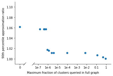
(a) Baden-Württemberg

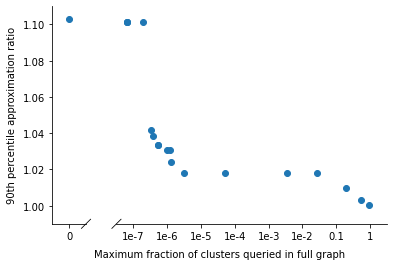
(b) Washington

Figure 1: The relationship between the maximum fraction of clusters probed among the queries and the approximation ratio obtained. Note that only a small fraction of clusters need to be probed to obtain a big improvement in approximation.

We assessed the efficacy of probing by studying statistics of the probed and no-probed approximation ratios for the 100 queries. In Baden-Württemberg,

1. 90 out of 100 of all query pairs had a probed approximation ratio below 1.012 (i.e. 1.2% distortion), with an average of .01% of all clusters probed per query pair.

2. the 90th out of 100 of all query pairs had a no-probe approximation ratio of 1.061 (i.e. 6.1% distortion)

In Washington,

1. 90 out of 100 of all query pairs had a probed approximation ratio below 1.018 (i.e. 1.8% distortion), with an average of .34% of all clusters probed per query pair.

2. the 90th out of 100 of all query pairs had a no-probe approximation ratio of 1.103 (i.e. 10.3% distortion)

Thus, in both cases, a small percentage of clusters results in a much shorter path as measured in the real traffic graph in both Washington and Baden-Württemberg.

5 Conclusion

Path search is a fundamental problem in computer science. In many applications – like finding driving directions in road networks – edge weights are inherently hidden. Thus, we would like to find shortest paths with as few queries to real edge weights as possible. In this work, we modeled traffic using random, possibly correlated, edge weights and observed that we could (a) approximate the $s-t$ traffic-aware distance or (b) compute an approximate traffic-aware $s-t$ path with a small number of queries under certain realistic assumptions. Even better, (a) can be done in a small amount of runtime. Furthermore, we observed that these assumptions are fundamentally required in order to be able to find paths with a small number of queries, theoretically speaking. Experimentally, though, we observed that these results are quite pessimistic.

In future work, it would be great to turn these observations into practical data structures for answering shortest path queries with traffic using no or little preprocessing. CRP (Delling et al., 2011) requires work to recompute shortcuts whenever edge weights in a cluster change. One could avoid that by clustering the graph into correlated pieces (highways) and applying our algorithm for correlated costs.

It would also be interesting to generalize the observations in this paper to other optimization problems. Our proof is quite simple and is not inherently tied to the shortest path problem. This could lead to simpler dynamic data structures for many problems when uncertainty in the input is random rather than adversarial.

Acknowledgements

We would like to thank Pachara Sawettamalaya for pointing us to Talagrand’s inequality in (Zhao, 2020).

Appendix A Appendix: Missing Proofs and Definitions

In this section, we provide the missing proofs and definitions.

A.1 Approximate Traffic Distance Data Structure

See 1.1

We now give the data structure ApproxTrafficDistance. Recall that Algorithm 1 probes all edges in the required neighborhood with weight above a certain threshold and computes the $s-t$ distance in the graph $H$ obtained by sampling a fresh copy of $G^{\prime}$ (the graph $G^{\prime\prime}$) and substituting the probed edge weights. This algorithm can be slow due to the call to Dijkstra on $H$. Instead, one can call a distance oracle on $G^{\prime\prime}$ with the probed edges deleted from the graph. This contains all of the information needed from $G^{\prime\prime}$. To compute the $s-t$ distance in $G^{\prime}$, make a graph $I$ consisting of $s,t$, and the endpoints of all probed edges with non-probed edges weighted by the length of the shortest path that does not use any probed edge. $I$ has at most $O(K_{0})$ vertices, so running Dijkstra on this graph is fast.

Algorithm 2 The data structure ApproxTrafficDistance in Theorem 1.1.

procedure PreprocessApproxTrafficDistance ($\mathcal{D},G,G^{\prime},\epsilon$)

     $w^{\prime\prime}\sim\mathcal{D}$

     $G^{\prime\prime}\leftarrow(V,E,w^{\prime\prime})$

     PreprocessApproxNoTrafficDistance($G,\epsilon/10$)

     for $i\in[\log(\min_{f}w_{f}),\log(\max_{f}w_{f})]$ do

         $E_{i}\leftarrow e\in E(G)$ for which $w_{e}>c\epsilon^{2}2^{i}/(\rho^{4}\log n)$

         $G_{i}^{\prime\prime}\leftarrow G^{\prime\prime}\backslash E_{i}$

         PreprocessApproxNoTrafficDistance($G_{i}^{\prime\prime},\epsilon/10$)

         $\mathcal{F}_{i}\leftarrow\text{sparse coverfor }\{B_{u}^{G}(\rho 2^{i})\}_{u\in V(G)}$

         for $S\in\mathcal{F}_{i}$ do

              $E_{S}\leftarrow E_{i}\cap G[S]$

         end for

     end for

end procedure

procedure QueryApproxTrafficDistance ($s,t,\mathcal{D},G,G^{\prime}$)

     $L\leftarrow$QueryApproxNoTrafficDistance($s,t,G$)

     $i\leftarrow\log L$

     $S\leftarrow$ a set in $\mathcal{F}_{i}$ that contains all of $B_{s}^{G}(100\rho 2^{i})$ (exists by definition of sparse cover)

     $X\leftarrow\{s,t\}\cup\{\text{endpoints of edges in $E_{S}$}\}$

     $I\leftarrow$ complete directed graph on $X$, where $w^{I}_{uv}\leftarrow$QueryApproxNoTrafficDistance($u,v,G_{i}^{\prime\prime}$) for all $u,v\in X$

     for $e\in E_{S}$ do

         $w^{I}_{e}\leftarrow\min(w^{\prime}_{e},w^{I}_{e})$

     end for

     return $d_{I}(s,t)$

end procedure

Proof of Theorem 1.1.

We first bound the runtime of the algorithm. For preprocessing, computing $w^{\prime\prime}$ and $G^{\prime\prime}$ takes $O(m)$ time and preprocessing the no-traffic data structure on $G$ takes $O(K_{1})$ time. Computing all $E_{i}$s and $G_{i}^{\prime\prime}$s takes $\tilde{O}(m)$ time, as this is only done $\log((\max_{f}w_{f})/(\min_{f}w_{f}))$ times, for a total of $O(m\log((\max_{f}w_{f})/(\min_{f}w_{f})))=\tilde{O}(m)$ time. Computing each $\mathcal{F}_{i}$ takes $\tilde{O}(m)$ time by [Miller et al., 2013], for a total of $\tilde{O}(m)$ time. Preprocessing the $G_{i}^{\prime\prime}$ data structures takes $\tilde{O}(K_{1})$ time. Computing all of the sets $E_{S}$ takes $\tilde{O}(m)$ by the degree property of the sparse cover; specifically computing $E_{S}$ takes $O(|E(G[S])|)$ time, so the total work for $\mathcal{F}_{i}$ is

$$\sum_{S\in\mathcal{F}_{i}}O(|E(G[S])|) =\sum_{S\in\mathcal{F}_{i}}\sum_{e\in E(G[S])}O(1)$$

$$=\sum_{e\in E(G)}O(\text{number of $S\in\mathcal{F}_{i}$ with $e\in E(G[S])$})$$

$$\leq\sum_{e\in E(G)}O\left((\log n)n^{1/(\log n)}\right)$$

$$=\tilde{O}(m).$$

This completes the preprocessing time bound. For query time, computing $L$ takes $K_{2}$ time, $i$ takes $O(1)$ time, and $S$ takes $O(1)$ time, as only a pointer to $S$ needs to be stored. Since $|E_{S}|\leq K_{0}$ by the radius bound of the sparse cover, constructing $I$ takes $\tilde{O}(K_{0}^{2}K_{2})$ time. Substituting the probed edge weights takes $K_{0}$ time and running Dijkstra in $I$ takes $\tilde{O}(K_{0}^{2})$ time. Thus, the total query time is $\tilde{O}(K_{0}^{2}K_{2})$, as desired.

Now, we bound the approximation error of the returned number. By Theorem 1, the shortest path in $G_{i}^{\prime\prime}$ with probed edges from $G^{\prime}$ added is a $(1+\epsilon/10)$-approximation to the shortest path in $G^{\prime}$. Let $v_{0}=s,v_{1},v_{2},\ldots,v_{k-1},v_{k}=t$ denote the subsequence of vertices visited by the path that are also in $I$. If $\{v_{i},v_{i+1}\}\in E_{S}$, then the probed value from $G^{\prime}$ is present in $I$. If $\{v_{i},v_{i+1}\}\notin E_{S}$, then the subpath between $v_{i}$ and $v_{i+1}$ does not use any probed edge, so the $v_{i}-v_{i+1}$ subpath is also a shortest path in $G_{i}^{\prime\prime}$. This means that $w_{v_{i}v_{i+1}}^{I}$ is a $(1+\epsilon/10)$-approximation to the length of the subpath, so the shortest path in $I$ is a $(1+\epsilon/10)^{2}<(1+\epsilon)$-approximation to the length of the shortest path in $G^{\prime}$, as desired.

∎

A.2 Definition of Highway Dimension

We use $P(v,w)$ to denote the shortest path between a pair of vertices $v$ and $w$. The definition of highway dimension is as follows:

Definition (Highway Dimension [Abraham et al., 2010]).

Given a graph $G=(V,E)$, the highway dimension of $G$ is the smallest integer $h$ such that

$$\forall\,r\in\mathbb{R}^{+},\forall u\in V,\exists S\subseteq B_{u,4r},|S|\leq h,\text{ such that }$$

$$\forall\,v,w\in B_{u,4r},\text{ if }|P(v,w)|>r\text{ and }P(v,w)\subseteq B_{u,4r},$$

$$\quad\text{ then }P(v,w)\cap S\neq\emptyset.$$

Similar as the continuous double dimension, we also define the continuous highway dimension of a graph by chopping each edge into infinitely many smaller segments:

Definition (Continuous Highway Dimension).

Consider a graph $G$. For a value $k$, replace each edge with a path of length $k$ to obtain a graph $G_{k}$, where each new edge has a weight equal to $1/k$ times the original weight. The continuous highway dimension of $G$ is defined to be the limit as $k$ goes to infinity of the highway dimension of $G_{k}$.

The continuous highway dimension can be used to upper bound the continuous doubling dimension (see Definition 3.2), by the following lemma:

Lemma A.1 (Upper bound of continuous doubling dimension).

If a graph $G$ has continuous doubling dimension $\alpha$ and continuous highway dimension $h$, we have $2^{\alpha}\leq h$.

Proof.

Omitted. See Claim 1 in [Abraham et al., 2010] for the proof. ∎

A.3 Algorithm of Probing Demands

See Algorithm 3 for the algorithm.

Algorithm 3 Algorithm when edge weights come from flows/can be correlated

procedure ProbingDemands
($s,t,G,\{\mathcal{D}_{i}\}_{i\in[m]},\{\lambda_{i}\}_{i\in[m]},\{\lambda_{i}^{e}\}_{i\in[m],e\in E},{\bm{y}}$)

     for $i\in[m],e\in E$ do

         $\tilde{w}_{e}\leftarrow w_{e}\cdot\left(\sum_{i\in[m]}\left(\lambda_{i}^{e}\cdot\lambda_{i}\right)\right)^{\beta}$

     end for

     $\tilde{G}\leftarrow(V,E,\tilde{w})$ $\triangleright$ Compute the edge weights under basic demands

     $L\leftarrow d_{\tilde{G}}(s,t)$

     $H\leftarrow\tilde{G}[\tilde{G}\cap B^{\tilde{G}}_{s}(\rho^{\beta}\cdot L)]$

     for $i\in[m]$ do

         $\Omega_{i}\leftarrow\sum_{e\in E_{H}\cap C_{i}}\tilde{w}_{e}$ $\triangleright$ Compute the cluster size of demand $y_{i}$

         if $\Omega_{i}>\frac{{\epsilon}^{2}\cdot L}{16\cdot\log 2n\cdot\rho^{3\beta}\cdot\ell}$ then

              $y^{\prime}_{i}\leftarrow y_{i}$ $\triangleright$ Probe on $y_{i}$ if the effective size is large

         else

              $y^{\prime}_{i}\sim\mathcal{D}_{i}$ $\triangleright$ Sample from $\mathcal{D}_{i}$ otherwise

         end if

     end for

     for $e\in E_{H}$ do

         $w_{e}^{H}\leftarrow\left(\sum_{i=1}^{m}\lambda_{i}^{e}\cdot y_{i}^{\prime}\right)^{\beta}\cdot w_{e}$

     end for

     return $d_{H}(s,t)$

end procedure

A.4 Concentration of Shortest Path Lengths

Here, we prove Lemma 3.4 that is used to establish our main results, restated as follows: See 3.4

Proof.

For our proof, we will need the following version of Talagrand’s concentration inequality.

Theorem A.2 (Theorem 9.4.14 of [Zhao, 2020]).

Let $\Omega=\Omega_{1}\times\cdots\times\Omega_{k}$ equipped with the product measure. Let $f:\Omega\to\mathbb{R}$ be a function. Suppose for every $x\in\Omega$, there is some $\alpha(x)\in\mathbb{R}_{\geq 0}^{k}$ such that for every $y\in\Omega$,

$$f(x)\leq f(y)+d_{\alpha(x)}(x,y).$$

where $d_{\alpha(x)}(x,y)=\sum\alpha_{i}1_{x_{i}\neq y_{i}}$ is the weighted Hamming distance. Then, for every $t\geq 0$,

$$\Pr(|f-\mathbb{M}f|\geq t)\leq 4\exp\left(\frac{-t^{2}}{4\sup_{x\in\Omega}|\alpha(x)|^{2}}\right)$$

where $\mathbb{M}X$ is the median for the random variable $X$; i.e., $\Pr(X\geq\mathbb{M}X)\geq 1/2$ and $\Pr(X\leq\mathbb{M}X)\leq 1/2$.

We will apply Theorem A.2 to show that the length of the shortest path is concentrated around its median. Here, $\Omega$ is the joint distribution of hidden variables $\mathcal{D}^{\prime}$ and $\Omega_{i}$ is the distribution of the hidden variable $y_{i}$.

We show that the condition for Theorem A.2 holds for $f:=-\delta$ with the following. For any weight vector ${\bm{y}}$ and ${\bm{x}}$ drawn from $\mathcal{D}^{\prime}$, let $p_{\bm{y}}$ (resp. $p_{\bm{x}}$) be the shortest path from $s$ to $t$ in $G_{\bm{y}}=(V,E,\{w_{e}\cdot f_{e}({\bm{y}})\}_{e\in E})$ (resp. $G_{\bm{x}}=(V,E,\{w_{e}\cdot f_{e}({\bm{x}})\}_{e\in E})$) and define $\alpha({\bm{x}})_{i}=(\rho^{\prime}-1)\cdot\sum_{e\in p_{\bm{x}}\cap C_{i}}w_{e}$ if $c_{i}<W$; and $0$ otherwise. We have

$$\delta({\bm{y}})\leq\sum_{e\in p_{\bm{x}}}w_{e}\cdot f_{e}({\bm{y}})=\sum_{e\in p_{\bm{x}}}w_{e}\cdot f_{e}({\bm{x}})+\sum_{e\in p_{\bm{x}}}w_{e}\cdot(f_{e}({\bm{y}})-f_{e}({\bm{x}})).$$

We partition the set $\{e:e\in p_{\bm{x}}\}$ into two parts. The first part $E_{1}$ consists the edges whose dependent variables remain the same as ${\bm{y}}$, i.e. $E_{1}=\{e\in p_{\bm{x}}:\forall i,e\in C_{i}\rightarrow x_{i}=y_{i}\}$. The rest edges are in $E_{2}$: $E_{2}=\{e\in p_{\bm{x}}:\exists\,i,e\in C_{i},x_{i}\neq y_{i}\}$. We have

$$\delta({\bm{y}}) =\delta({\bm{x}})+\sum_{e\in E_{1}}w_{e}\cdot(f_{e}({\bm{y}})-f_{e}({\bm{x}}))+\quad\quad\sum_{e\in E_{2}}w_{e}\cdot(f_{e}({\bm{y}})-f_{e}({\bm{x}}))$$

$$=\delta({\bm{x}})+\sum_{e\in p_{\bm{x}}:\exists\,i,e\in C_{i},x_{i}\neq y_{i}}w_{e}\cdot(f_{e}({\bm{y}})-f_{e}({\bm{x}}))$$

$$\leq\delta({\bm{x}})+\sum_{i:x_{i}\neq y_{i}}\sum_{e\in p_{\bm{x}}\cap C_{i}}w_{e}\cdot(\rho^{\prime}-1)$$

$$=\delta({\bm{x}})+d_{\alpha({\bm{x}})}({\bm{x}},{\bm{y}}).$$

Observe that

$$\sup_{{\bm{x}}}|\alpha({\bm{x}})|^{2} =\sup_{{\bm{x}}}\sum_{i=1}^{m}{|\alpha({\bm{x}})_{i}|^{2}}$$

$$\leq\sup_{{\bm{x}}}\left(\sum_{i=1}^{m}{|\alpha({\bm{x}})_{i}|}\right)\cdot\sup_{{\bm{x}},i}\alpha({\bm{x}})_{i}$$

$$\leq\rho^{\prime}\cdot\sup_{{\bm{x}}}\delta({\bm{x}})\cdot\ell\cdot(\rho^{\prime}-1)\cdot\sup_{{\bm{x}},i}\alpha({\bm{x}})_{i}$$

$$\leq\rho^{\prime}\cdot\sup_{{\bm{x}}}\delta({\bm{x}})\cdot\ell\cdot(\rho^{\prime}-1)^{2}\cdot W.$$

Applying Theorem A.2, we have

$$\Pr(|\delta(x)-\mathbb{M}\delta|\geq\tau)\leq 4\exp{\left(\frac{-\tau^{2}}{4\rho^{\prime}(\rho^{\prime}-1)^{2}\cdot W\cdot\ell\cdot\sup_{\bm{z}}\delta({\bm{z}})}\right)}.$$

The theorem then follows by plugging in $\tau/2$ and applying a union bound. ∎

A.5 Bounds on the Intersected Large Clusters

See 3.5

Proof.

We first prove that an $r$-radius ball can only intersect with $h^{2}\cdot\ell$ different clusters with total weight in the range $(r,\ \infty)$. If a path is intersecting the $r$-radius ball and has total length larger than $r$, it must contain a subset of edges with total weight greater than $r$ that form a shortest path inside the $4r$-radius ball centered at $s$. By the definition of the highway dimension, the shortest path inside the $4r$-radius ball contains at least one of the highway points. By the third property, we know that each highway point inside an edge (not vertex) is covered by at most $\ell$ different clusters. A highway point on a vertex $v$ falls on at most $\ell\cdot d(v)$ different clusters, where $d(v)$ is the degree of the vertex $v$. Denote the continuous doubling dimension of the graph by ${\alpha}$, we have ${\alpha}\leq\log h$ (by Lemma A.1). Since we have $2^{{\alpha}}$ as an upper bound of the degree of a vertex, we have $d(v)\leq h$. Therefore, the $r$ radius ball will intersect with at most $h^{2}\cdot\ell$ clusters with size in the range $(r,\ \infty)$.

Since the continuous doubling dimension of $G$ is bounded by $\log h$, we can cover the $R$-radius ball with $h^{\lceil\log R/r\rceil}$ $r$-radius balls. Let $r=\Gamma$. Each $r$-radius ball intersects with at most $h^{2}\cdot\ell$ $\Gamma$-large clusters, the total number of $\Gamma$-large clusters intersecting with the $R$-radius ball is at bounded by $h^{\lceil\log R/\Gamma\rceil}\cdot h^{2}\cdot\ell\leq h^{3}\cdot\ell\cdot\left(\frac{R}{\Gamma}\right)^{\log h}$. ∎

A.6 Finding a Short Path in $G^{\prime}$ Requires Lots of Probes

In Section 3, we showed that the $s-t$ distance in the real graph $G^{\prime}$ can be approximated using a small number of probes to edge weights in $G^{\prime}$. Even better, these probes are done non-adaptively; i.e. the edges are probed in one batch. One may wonder whether it is possible to always produce a short path in $G^{\prime}$. By short path, we mean the path whose length is approximately equal to the shortest path between $s$ and $t$. We show that this is indeed impossible, even with a large number of adaptively chosen probes. In order to formally describe the result, we first need to define adaptive probing strategies:

Definition A.3 (Adaptive probing strategies).

Consider a hidden graph $G^{\prime}$. An adaptive probing strategy is an algorithm $\mathcal{A}$ that takes a pair $(s,t)$ of vertices in $G^{\prime}$ along with the unweighted edges of $G^{\prime}$ and outputs an $s-t$ path $P$. The algorithm is also given the weights of some edges in $G^{\prime}$, given as follows. The algorithm picks a sequence of edges $e_{1},e_{2},\ldots,e_{k}$ and sees their edge weights $w_{1},w_{2},\ldots,w_{k}$ respectively in $G^{\prime}$. The choice of the $e_{i}$s is allowed to be adaptive, in the sense that the choice of $e_{i}$ is a function of $s,t$, and $w_{1},w_{2},\ldots,w_{i-1}$.

The query complexity of the algorithm $\mathcal{A}$ is the number $k$. The quality of the path $P$, denoted $q(P)$, is the ratio $q(P):=\ell_{G^{\prime}}(P)/d_{G^{\prime}}(s,t)$, where $\ell_{G^{\prime}}(P)$ denotes the length of $P$ in $G^{\prime}$.

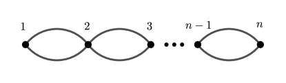
Figure 2: High-query example for finding a path in $G^{\prime}$

In the following proof, we set $\rho$ to be $2$ for simplicity. We can scale the edge weight easily by considering $1+(w_{e}-1)\cdot(\rho-1)$ instead, and the same result still follows.

We now define an example graph in which it is hard to find a short path using an adaptive probing strategy. This example is depicted in Figure 2. Make an $n$-vertex graph $G$ with vertices $v_{1},v_{2},\ldots,v_{n}$. Between any two consecutive vertices $v_{i},v_{i+1}$, there are two edges $e_{i}$ and $f_{i}$. A hidden graph $G^{\prime}$ is generated by giving edge weights to each of the edges in $G$. For $e_{i}$ and $f_{i}$, the edge weights are denoted $u_{i}$ and $l_{i}$ respectively. The $u_{i}$s and $l_{i}$s are sampled uniformly and independently from the interval $[1,2]$ as usual. When $G$ and $G^{\prime}$ are used in this subsection, they will always refer to the graphs $G$ and $G^{\prime}$ defined in this paragraph.

Now, consider an adaptive probing strategy $\mathcal{A}$. We will ask it to compute a path between $s=v_{1}$ and $t=v_{n}$. Note the following:

Proposition A.4.

$d_{G^{\prime}}(s,t)=\sum_{i=1}^{n-1}\min(u_{i},l_{i})$.

Proof.

Any path from $s$ to $t$ uses exactly one edge from the set $\{e_{i},f_{i}\}$ for each $i$. Therefore, $d_{G^{\prime}}(s,t)\geq\sum_{i=1}^{n-1}\min(u_{i},l_{i})$. The minimum weight edges, though, also yield a path from $s$ to $t$, so $d_{G^{\prime}}(s,t)\leq\sum_{i=1}^{n-1}\min(u_{i},l_{i})$ as well, as desired. ∎

Throughout our analysis, we use the classic Chernoff-Hoeffding bound:

Theorem A.5 (Hoeffding’s inequality).

Let $X_{1},\dots,X_{n}$ be independent random variables such that $a_{i}\leq X_{i}\leq b_{i}$ for all $i$. Let $X=\sum_{i=1}^{n}X_{i}$. Then,

$$\Pr(|X-\mathbb{E}[X]|\geq t)\leq 2\exp\left(-\frac{2t^{2}}{\sum_{i=1}^{n}(b_{i}-a_{i})^{2}}\right)$$

for all $t>0.$

We use Chernoff to upper bound the denominator of the quality value:

Proposition A.6.

With probability at least $1-1/n^{100}$, $d_{G^{\prime}}(s,t)\leq 4n/3+n/100$.

Proof.

We apply Chernoff with $X_{i}=\min(u_{i},l_{i})\in[1,2]$. Thus, by Theorem A.5,

$$\Pr\big{(}|X-\mathbb{E}[X]|\geq n/100\big{)}\leq 2e^{-\Theta(n)}\leq n^{-100}.$$

Furthermore, $\mathbb{E}[X_{i}]=4/3$ for all $i$, because

$$\mathbb{E}[X_{i}] =\int_{1}^{2}(\Pr[X_{i}>x]+1)dx$$

$$=1+\int_{1}^{2}\Pr(u_{i}>x)\Pr(l_{i}>x)dx$$

$$=1+\int_{1}^{2}(2-x)^{2}dx$$

$$=4/3.$$

Thus, $\mathbb{E}[X]\leq 4n/3$, which means that $d_{G^{\prime}}(s,t)=X\leq 4n/3+n/100$ with probability at least $1-1/n^{100}$ as desired. ∎

Thus, to get a lower bound on the quality (approximation ratio), we just need to lower bound the numerator. We show the following:

Lemma A.7.

Any adaptive probing strategy with query complexity at most $n/100$ outputs a path $P$ with $\ell_{G^{\prime}}(P)\geq 3n/2-n/20$ with probability at least $1-1/n^{100}$.

Proof.

Let $\mathcal{A}$ be an adaptive probing strategy with query complexity $k$ for some $k\leq n/100$. The probed values $w_{1},w_{2},\ldots,w_{k}$ are random variables. Consider some fixing of these random variables. This fixing induces a fixed choice of edges $g_{1},g_{2},\ldots,g_{k}$ queried by the algorithm and a choice of one path $P$. Let $S\subseteq\{1,2,\ldots,n-1\}$ be the minimum set of indices for which $g_{1},g_{2},\ldots,g_{k}\subseteq\cup_{i\in S}\{e_{i},f_{i}\}$. In particular, $|S|\leq k$ and for every $i\notin S$, neither $l_{i}$ nor $u_{i}$ were queried by $\mathcal{A}$.

For any $i$, let $h_{i}$ be the single edge among $\{e_{i},f_{i}\}$ that the path $P$ uses and let $X_{i}$ be the weight of $h_{i}$ in $G^{\prime}$ (either $l_{i}$ or $u_{i}$). The $X_{i}$s are random variables. Conditioned on $w_{1},w_{2},\ldots,w_{k}$, the $X_{i}$s for $i\notin S$ are independent because the choice of path $P$ is not a function of $l_{i}$ or $u_{i}$. Thus, we may apply Chernoff to lower bound their sum. By Theorem A.5,

$$\Pr\Bigg{(}\bigg{|}\sum_{i\notin S}X_{i}-\mathbb{E}\Big{[}\sum_{i\notin S}X_{i}\;|\;w_{1},\ldots,w_{k}\Big{]}\bigg{|}>n/50\;\Big{|}\;w_{1},\ldots,w_{k}\Bigg{)}\leq 2e^{-\Theta(n)}<n^{-100}.$$

Furthermore, for any $i\notin S$,

$$\mathbb{E}[X_{i}|w_{1},\ldots,w_{k}]=3/2$$

and because $|S|\leq k\leq n/100$,

$$\mathbb{E}\left[\sum_{i\notin S}X_{i}|w_{1},\ldots,w_{k}\right]=(3/2)(n-|S|-1)>3n/2-n/50.$$

Combining these statements shows that

$$\Pr\left(\sum_{i\notin S}X_{i}\leq 3n/2-n/20\Big{|}w_{1},\ldots,w_{k}\right)\leq n^{-100}.$$

By the tower law of conditional expectations,

$$\Pr\left(\sum_{i\notin S}X_{i}\leq 3n/2-n/20\right) =\mathbb{E}\left[\Pr\left(\sum_{i\notin S}X_{i}\leq 3n/2-n/20\Big{|}w_{1},\ldots,w_{k}\right)\right]$$

$$\leq\mathbb{E}[n^{-100}]$$

$$\leq n^{-100}.$$

By definition, it is always the case that $\ell_{G^{\prime}}(P)\geq\sum_{i\notin S}X_{i}$, so $\ell_{G^{\prime}}(P)>3n/2-n/20$ with probability at least $1-n^{-100}$, as desired. ∎

We are now ready to show the main lower bound:

See 1.3

Proof.

Lemma A.7 shows that $\ell(P)\geq 3n/2-n/20$ with probability at least $1-n^{-100}$ over the choice of edge weights in $G^{\prime}$. Proposition A.6 shows that $d_{G^{\prime}}(s,t)\leq 4n/3+n/100$ with probability at least $1-n^{-100}$ over the choice of $G^{\prime}$. Thus, by a union bound,

$$q(P)\geq(3n/2-n/20)/(4n/3-n/100)>9/8-1/10>1$$

with probability at least $1-2n^{-100}$, as desired. ∎

A.7 Getting around the lower bound

There is something very unrealistic about the Figure 2 example, though. Specifically, there are exponentially many possible shortest paths from $s$ to $t$. This does not make intuitive sense in road networks – such paths could only arise if a car exited and re-entered a highway a large number of times. Thus, the following assumption makes sense:

See 1

Mathematically, for any origin-destination pair $s-t$, let $S$ be a set of all possible graph $\tilde{G}=(V,E,\tilde{w})$ constructed by sampling $\tilde{w}\sim\mathcal{D}$, then the size of set of possible shortest paths $\{P_{\tilde{G}}(s,t)|\tilde{G}\in S\}$ is polynomial in $|V|$.

See 1.4 In the analysis, we make use of a one-sided McDiarmid’s Inequality:

Theorem A.8 (Theorem 6.1 of [Chung and Lu, 2006], with martingale given by sum of first $i$ variables and applied on negation to get two sidedness).

Let $X_{1},\ldots,X_{n}$ be independent random variables with $|X_{i}-\mathbb{E}[X_{i}]|\leq M$ for all $i$. Let $X=\sum_{i=1}^{n}X_{i}$. Then, for any $\lambda>0$,

$$\Pr[|X-\mathbb{E}[X]|\geq\lambda]\leq 2e^{-\frac{\lambda^{2}}{\sum_{i=1}^{n}\text{Var}(X_{i})+M\lambda/3}}.$$

Proof.

By the edge count bound of Theorem 1.2, the algorithm only probes $((\rho\log nU)/\epsilon)^{O(h)}$ edges, so it suffices to show that the algorithm finds an $(1+\epsilon)$-approximate path in $G^{\prime}$. By the polynomial paths assumption, the shortest $s-t$ path in $G^{\prime}$ is one of $U$ different paths $P_{1},P_{2},\ldots,P_{U}$. We start by showing that, with probability at least $1-4/((nU)^{100})$,

$$(1-\epsilon)\ell_{G^{\prime}}(P_{i})\leq\ell_{H}(P_{i})\leq(1+\epsilon)\ell_{G^{\prime}}(P_{i})$$

for each $i$. To do this, think about the construction of $H$ slightly differently. Think of the construction of $H$ as replacing the low edge weights in $G^{\prime}$ with edge weights in $G^{\prime\prime}$. In particular, all large edge weights are deterministic, and all small ones are randomized. Break the edges of $P_{i}$ into two sets $A$ and $B$, depending on whether their weight in $G^{\prime}$ (within a factor of $\rho$ of the same value for $G$) is greater than or less than $c\epsilon^{2}L/(\rho^{4}\log nU)$ respectively. Recall that $w_{e}^{\prime}$ and $w_{e}^{\prime\prime}$ denote the weights of $e$ in $G^{\prime}$ and $G^{\prime\prime}$ respectively. We now use Theorem A.8 to bound the error. Note that for $e\in B$,

$$\text{Var}(w_{e}^{\prime\prime}) \leq\mathbb{E}[(w_{e}^{\prime\prime})^{2}]$$

$$\leq\rho^{2}(w_{e}^{\prime})^{2}$$

$$\leq\rho^{2}(w_{e}^{\prime})\max_{f\in B}w_{f}^{\prime}$$

$$\leq w_{e}^{\prime}\cdot c\epsilon^{2}L/(\rho^{2}\log nU).$$

Therefore,

$$\sum_{e\in B}\text{Var}(w_{e}^{\prime\prime}) \leq\ell_{G^{\prime}}(P_{i})\cdot c\epsilon^{2}L/(\rho^{2}\log nU)$$

$$\leq c\epsilon^{2}L^{2}/(\rho\log nU)$$

since $\rho L\geq\ell_{G^{\prime}}(P_{i})$ (otherwise $P_{i}$ cannot be a candidate shortest path). Using $M=c\epsilon^{2}L/(\rho^{4}\log nU)$, $X_{e}=w_{e}^{\prime\prime}$ for all $e\in B$ and $X_{e}=w_{e}^{\prime}$ for all $e\in A$, and $\lambda=\epsilon L/2$ shows that

$$\Pr[|X-\mathbb{E}[X]|\geq\epsilon L/2]\leq 2/(nU)^{100}$$

where $X=\sum_{e\in A}w_{e}^{\prime}+\sum_{e\in B}w_{e}^{\prime\prime}$, which is also the length of $P_{i}$. This inequality also uses the fact that $c<1/800$. Notice that $G^{\prime}$ and $H$ are both samples from the distribution over edge weights that this probability bound pertains to. Thus,

$$\Pr[|\ell_{H}(P_{i})-\mathbb{E}[X]|\geq\epsilon L/2]\leq 2/(nU)^{100}$$

and

$$\Pr[|\ell_{G^{\prime}}(P_{i})-\mathbb{E}[X]|\geq\epsilon L/2]\leq 2/(nU)^{100}.$$

By Union bound,

$$\Pr[|\ell_{G^{\prime}}(P_{i})-\ell_{H}(P_{i})|\geq\epsilon\ell_{G^{\prime}}(P_{i})]\leq 4/(nU)^{100}$$

because $L\leq\ell_{G^{\prime}}(P_{i})$. This is the first desired probability bound. Now, we discuss how to use it to prove the theorem. Union bound over all $U$ paths to show that all of these inequalities hold simultaneously with probability at least $1-n^{-100}$. Let $P$ denote the shortest path in $G^{\prime}$. Applying the inequalities to $P_{i}=P$ shows that $P$ is only a $(1+\epsilon)$-factor longer in $H$. This means that the path $Q$ that the algorithm returns has length at most $(1+\epsilon)\ell_{G^{\prime}}(P)$. $Q$ is one of the $P_{i}$s, because it is the shortest path in $H$, which is a valid sample from the distribution that $G^{\prime}$ is sampled. Thus, we may apply the inequality to it to show that the length of $Q$ in $G^{\prime}$ is at most $\frac{1+\epsilon}{1-\epsilon}\cdot\ell_{G^{\prime}}(P)\leq(1+3\epsilon)\ell_{G^{\prime}}(P)$. Thus, $Q$ is a $(1+3\epsilon)$-approximate path in $G^{\prime}$ as desired. ∎

References

- Abraham et al. [2006] I. Abraham, C. Gavoille, A. V. Goldberg, and D. Malkhi. Routing in networks with low doubling dimension. In 26th IEEE International Conference on Distributed Computing Systems (ICDCS’06), pages 75–75. IEEE, 2006.
- Abraham et al. [2010] I. Abraham, A. Fiat, A. V. Goldberg, and R. F. Werneck. Highway dimension, shortest paths, and provably efficient algorithms. In Proceedings of the twenty-first annual ACM-SIAM symposium on Discrete Algorithms, pages 782–793. SIAM, 2010.
- Abraham et al. [2016] I. Abraham, D. Delling, A. Fiat, A. V. Goldberg, and R. F. Werneck. Highway dimension and provably efficient shortest path algorithms. Journal of the ACM (JACM), 63(5):1–26, 2016.
- Aldous [2016] D. J. Aldous. Weak concentration for first passage percolation times on graphs and general increasing set-valued processes. ALEA, 13:925–940, 2016.
- Auffinger et al. [2015] A. Auffinger, M. Damron, and J. Hanson. 50 years of first passage percolation. arXiv preprint arXiv:1511.03262, 2015.
- Awerbuch and Peleg [1990] B. Awerbuch and D. Peleg. Sparse partitions (extended abstract). In 31st Annual Symposium on Foundations of Computer Science, St. Louis, Missouri, USA, October 22-24, 1990, Volume II, pages 503–513. IEEE Computer Society, 1990. doi: 10.1109/FSCS.1990.89571. URL https://doi.org/10.1109/FSCS.1990.89571.
- Bast et al. [2006] H. Bast, S. Funke, and D. Matijevic. Transit ultrafast shortest-path queries with linear-time preprocessing. In 9th DIMACS Implementation Challenge, pages 175–192, 2006.
- Bast et al. [2007] H. Bast, S. Funke, D. Matijevic, P. Sanders, and D. Schultes. In transit to constant time shortest-path queries in road networks. In 2007 Proceedings of the Ninth Workshop on Algorithm Engineering and Experiments (ALENEX), pages 46–59. SIAM, 2007.
- Bauer and Delling [2010] R. Bauer and D. Delling. Sharc: Fast and robust unidirectional routing. Journal of Experimental Algorithmics (JEA), 14:2–4, 2010.
- Benita et al. [2020] F. Benita, V. Bilò, B. Monnot, G. Piliouras, and C. Vinci. Data-driven models of selfish routing: why price of anarchy does depend on network topology. In International Conference on Web and Internet Economics, pages 252–265. Springer, 2020.
- Bertsekas and Tsitsiklis [1991] D. P. Bertsekas and J. N. Tsitsiklis. An analysis of stochastic shortest path problems. Mathematics of Operations Research, 16(3):580–595, 1991.
- Bhaskara et al. [2020] A. Bhaskara, S. Gollapudi, K. Kollias, and K. Munagala. Adaptive probing policies for shortest path routing. Advances in Neural Information Processing Systems, 33:8682–8692, 2020.
- Bnaya et al. [2009] Z. Bnaya, A. Felner, and S. E. Shimony. Canadian traveler problem with remote sensing. In IJCAI, pages 437–442, 2009.
- Chung and Lu [2006] F. R. K. Chung and L. Lu. Survey: Concentration inequalities and martingale inequalities: A survey. Internet Math., 3(1):79–127, 2006. doi: 10.1080/15427951.2006.10129115. URL https://doi.org/10.1080/15427951.2006.10129115.
- Cohen et al. [2021] A. Cohen, Y. Efroni, Y. Mansour, and A. Rosenberg. Minimax regret for stochastic shortest path. Advances in neural information processing systems, 34:28350–28361, 2021.
- Çolak et al. [2016] S. Çolak, A. Lima, and M. C. González. Understanding congested travel in urban areas. Nature communications, 7(1):10793, 2016.
- Delling et al. [2011] D. Delling, A. V. Goldberg, T. Pajor, and R. F. Werneck. Customizable route planning. In Experimental Algorithms: 10th International Symposium, SEA 2011, Kolimpari, Chania, Crete, Greece, May 5-7, 2011. Proceedings 10, pages 376–387. Springer, 2011.
- Feldmann and Marx [2018] A. E. Feldmann and D. Marx. The parameterized hardness of the k-center problem in transportation networks. CoRR, abs/1802.08563, 2018. URL http://arxiv.org/abs/1802.08563.
- Geisberger et al. [2008] R. Geisberger, P. Sanders, D. Schultes, and D. Delling. Contraction hierarchies: Faster and simpler hierarchical routing in road networks. In Experimental Algorithms: 7th International Workshop, WEA 2008 Provincetown, MA, USA, May 30-June 1, 2008 Proceedings 7, pages 319–333. Springer, 2008.
- Goldberg and Harrelson [2005] A. V. Goldberg and C. Harrelson. Computing the shortest path: A* search meets graph theory. In SODA, volume 5, pages 156–165, 2005.
- Goldberg et al. [2006] A. V. Goldberg, H. Kaplan, and R. F. Werneck. Reach for a*: Efficient point-to-point shortest path algorithms. In 2006 Proceedings of the Eighth Workshop on Algorithm Engineering and Experiments (ALENEX), pages 129–143. SIAM, 2006.
- Gutman [2004] R. J. Gutman. Reach-based routing: A new approach to shortest path algorithms optimized for road networks. ALENEX/ANALCO, 4:100–111, 2004.
- Hilger et al. [2009] M. Hilger, E. Köhler, R. H. Möhring, and H. Schilling. Fast point-to-point shortest path computations with arc-flags. The Shortest Path Problem: Ninth DIMACS Implementation Challenge, 74:41–72, 2009.
- ich Lauther [2006] U. ich Lauther. An extremely fast, exact algorithm for finding shortest paths in static networks with geographical background. 2006.
- Kesten [1987] H. Kesten. Percolation theory and first-passage percolation. The Annals of Probability, 15(4):1231–1271, 1987.
- Kesten [1993] H. Kesten. On the speed of convergence in first-passage percolation. The Annals of Applied Probability, pages 296–338, 1993.
- Manual [1964] T. A. Manual. Bureau of public roads, us dept. Commerce, Urban Planning Division, Washington, DC, USA, 1964.
- Miller et al. [2013] G. L. Miller, R. Peng, and S. C. Xu. Parallel graph decompositions using random shifts. In G. E. Blelloch and B. Vöcking, editors, 25th ACM Symposium on Parallelism in Algorithms and Architectures, SPAA ’13, Montreal, QC, Canada - July 23 - 25, 2013, pages 196–203. ACM, 2013. doi: 10.1145/2486159.2486180. URL https://doi.org/10.1145/2486159.2486180.
- Nikolova and Karger [2008] E. Nikolova and D. R. Karger. Route planning under uncertainty: The canadian traveller problem. In AAAI, pages 969–974, 2008.
- OpenStreetMap contributors [2017] OpenStreetMap contributors. Planet dump retrieved from https://planet.osm.org , available under Open Database License. https://www.openstreetmap.org, 2017.
- Papadimitriou and Yannakakis [1991] C. H. Papadimitriou and M. Yannakakis. Shortest paths without a map. Theoretical Computer Science, 84(1):127–150, 1991.
- Rosenberg and Mansour [2019] A. Rosenberg and Y. Mansour. Online stochastic shortest path with bandit feedback and unknown transition function. Advances in Neural Information Processing Systems, 32, 2019.
- Rosenberg et al. [2020] A. Rosenberg, A. Cohen, Y. Mansour, and H. Kaplan. Near-optimal regret bounds for stochastic shortest path. In International Conference on Machine Learning, pages 8210–8219. PMLR, 2020.
- Sanders and Schultes [2005] P. Sanders and D. Schultes. Highway hierarchies hasten exact shortest path queries. In ESA, volume 3669, pages 568–579. Springer, 2005.
- Schultes and Sanders [2007] D. Schultes and P. Sanders. Dynamic highway-node routing. In Experimental Algorithms: 6th International Workshop, WEA 2007, Rome, Italy, June 6-8, 2007. Proceedings 6, pages 66–79. Springer, 2007.
- Steif [2009] J. E. Steif. A survey of dynamical percolation. In Fractal geometry and stochastics IV, pages 145–174. Springer, 2009.
- Tarbouriech et al. [2021] J. Tarbouriech, R. Zhou, S. S. Du, M. Pirotta, M. Valko, and A. Lazaric. Stochastic shortest path: Minimax, parameter-free and towards horizon-free regret. Advances in neural information processing systems, 34:6843–6855, 2021.
- Zhao [2020] Y. Zhao. Probabilistic methods in combinatorics, 2020. URL https://yufeizhao.com/pm/fa20/probmethod_notes.pdf.
- Zhu et al. [2013] A. D. Zhu, H. Ma, X. Xiao, S. Luo, Y. Tang, and S. Zhou. Shortest path and distance queries on road networks: towards bridging theory and practice. In Proceedings of the 2013 ACM SIGMOD International Conference on Management of Data, pages 857–868, 2013.