Simulations of stochastic fluid dynamics near a critical point in the phase diagram

Abstract

We present simulations of stochastic fluid dynamics in the vicinity of a critical endpoint belonging to the universality class of the Ising model. This study is motivated by the challenge of modeling the dynamics of critical fluctuations near a conjectured critical endpoint in the phase diagram of Quantum Chromodynamics (QCD). We focus on the interaction of shear modes with a conserved scalar density, which is known as model H. We show that the observed dynamical scaling behavior depends on the correlation length and the shear viscosity of the fluid. As the correlation length is increased or the viscosity is decreased we observe a cross-over from the dynamical exponent of critical diffusion, $z\simeq 4$, to the expected scaling exponent of model H, $z\simeq 3$. We use our method to investigate time-dependent correlation function of non-Gaussian moments $M^{n}(t)$ of the order parameter. We find that the relaxation time depends in non-trivial manner on the power $n$.

I Introduction

The transition from hadronic matter to a quark gluon plasma along the finite temperature axis in the QCD phase diagram is known to be a smooth crossover Aoki et al. (2006). As the baryon doping is increased, this crossover may turn into a first-order phase transition at a critical endpoint Stephanov et al. (1998). Experimental searches for critical behavior have focused on a possible non-monotonic dependence of fluctuation observables, such as the cumulants of conserved charges, on the beam energy Bzdak et al. (2020); Bluhm et al. (2020); An et al. (2022); Adam et al. (2021). Understanding the dynamical evolution of these observables in a heavy ion collision requires a hydrodynamic theory that incorporates the effects of fluctuations Rajagopal and Wilczek (1993); Berdnikov and Rajagopal (2000); Son and Stephanov (2004).

Theories of this type were first classified by Hohenberg and Halperin Hohenberg and Halperin (1977). They include purely relaxational dynamics (model A) Schweitzer et al. (2020); Schäfer and Skokov (2022), the diffusive dynamics of a conserved charge (model B) Berdnikov and Rajagopal (2000); Nahrgang et al. (2019); Schweitzer et al. (2022), and the diffusive evolution of an order parameter field advected by the momentum density of the fluid (model H). Model H is expected to govern the dynamics near a possible critical endpoint in the QCD phase diagram Son and Stephanov (2004).

Stochastic hydrodynamic theories have been studied using a variety of methods Mukherjee et al. (2015); Akamatsu et al. (2017); Stephanov and Yin (2018); Martinez and Schäfer (2019); Akamatsu et al. (2019); An et al. (2019, 2020, 2021), but there is little work on direct numerical simulation (see Berges et al. (2010); Nahrgang et al. (2019); Schweitzer et al. (2020, 2022); Pihan et al. (2023); Schäfer and Skokov (2022) for exceptions). In particular, model H has not been studied numerically. This is related to the fact that numerical simulations face a number of obstacles, including the need to regularize and renormalize short-distance noise, the requirement to implement fluctuation-dissipation relations, and the necessity to resolve ambiguities in the definition of stochastic partial differential equations.

In the present work, we describe a numerical implementation of model H using a Metropolis method previously applied to models A, B and G (chiral dynamics) Florio et al. (2022); Schäfer and Skokov (2022); Chattopadhyay et al. (2023); Florio et al. (2023). The novel feature of model H compared to purely relaxational or diffusive theories is the presence of “mode couplings” or “Poisson-brackets”. These terms describe advective interactions that conserve the hydrodynamic Hamiltonian, but lead to non-linear mode couplings between shear waves and the diffusive evolution of the order parameter. In the following, we introduce the model, explain our numerical approach, present a number of consistency checks, and then present results for the dynamical evolution of non-Gaussian moments. We comment on other applications and possible extensions of our methods.

II Model H

Model H is defined by Hohenberg and Halperin (1977); Folk and Moser (2006)

$$\partial_{t}\phi =\Gamma\,\nabla^{2}\left(\frac{\delta{\cal H}}{\delta\phi}\right)-\left(\vec{\nabla}\phi\right)\frac{\delta{\cal H}}{\delta\vec{\pi}_{T}}+\zeta,$$ (1)

$$\partial_{t}\pi^{T}_{i} =\eta\nabla^{2}\left(\frac{\delta{\cal H}}{\delta\pi^{T}_{i}}\right)+P^{T}_{ij}\left[\left(\nabla_{j}\phi\right)\frac{\delta{\cal H}}{\delta\phi}\right]$$

$$\hskip 42.67912pt-P^{T}_{ij}\left[\nabla_{k}\left(\pi^{T}_{j}\frac{\delta{\cal H}}{\delta\pi^{T}_{k}}\right)\right]+\xi_{i}\,,$$ (2)

where $\phi$ is the order parameter density, $\vec{\pi}$ is the momentum density of the fluid, $\Gamma$ and $\eta$ are transport coefficients . We can take $\phi$ to be proportional to the specific entropy $s/n$ of the fluid Akamatsu et al. (2019); An et al. (2023). $\Gamma$ is the thermal diffusivity, and $\eta$ is the shear viscosity. The transverse projection operator is given by

$$P^{T}_{ij}=\delta_{ij}-\frac{\nabla_{i}\nabla_{j}}{\nabla^{2}}$$ (3)

and $\pi^{T}_{i}=P^{T}_{ij}\pi_{j}$. The Hamiltonian (the free energy functional) is given by

$${\cal H}=\int d^{d}x\left[\frac{1}{2\rho}(\vec{\pi}_{T})^{2}+\frac{1}{2}(\nabla\phi)^{2}+\frac{m_{0}^{2}}{2}\phi^{2}+\frac{\lambda}{4}\phi^{4}-h\phi\right],$$ (4)

where $\rho$ is the mass density (the density of enthalpy in the relativistic case), $m_{0}$ is the bare inverse correlation length, $\lambda$ is a non-linear self-coupling, and $h$ is an external field. In practical applications, these parameter can be mapped onto the chemical potential-temperature $(\mu,T)$ plane, see for example Parotto et al. (2020); Kahangirwe et al. (2024). The noise terms $\zeta$ and $\xi_{i}$ are random fields constrained by fluctuation-dissipation relations. The noise correlation functions are given by

$$\langle\zeta(t,\vec{x})\zeta(t^{\prime},\vec{x}^{\prime})\rangle =-2T\,\Gamma\,\nabla^{2}\delta(\vec{x}-\vec{x}^{\prime})\delta(t-t^{\prime})\,,$$ (5)

$$\langle\xi_{i}(t,\vec{x})\xi_{j}(t^{\prime},\vec{x}^{\prime})\rangle =-2T\,\eta\,P^{T}_{ij}\nabla^{2}\delta(\vec{x}-\vec{x}^{\prime})\delta(t-t^{\prime})\,.$$ (6)

Note that equations (1,II) describe the interaction of shear modes with the order parameter, but they do not include sound modes. This truncation is expected to be sufficient to describe the critical dynamics of the fluid Hohenberg and Halperin (1977); Son and Stephanov (2004), but for other applications it will be interesting to include the coupling to longitudinal modes Martinez et al. (2019).

III Numerical method

In order to study the theory numerically, we discretize the fields $\phi(\vec{x})$ and $\vec{\pi}(\vec{x})$ on a $d$-dimensional lattice $\vec{x}=\vec{n}a$ with $n_{i}=1,\ldots,N$. In the following, we will focus on $d=3$. The main idea underlying the algorithm we employ is that the dissipative and stochastic updates are combined into a single Metropolis step. This method ensures that fluctuation-dissipation relations are satisfied and that the fluid equilibrates to a state in which the fields $\phi(\vec{x})$ and $\vec{\pi}^{T}(\vec{x})$ are sampled from the distribution $\exp(-{\cal H}/T)$. The Metropolis step is followed by a deterministic step that implements the non-dissipative mode coupling terms.

The Metropolis update for the field $\phi$ is given by

$$\phi^{\rm trial}(\vec{x},t+\Delta t) =\phi(\vec{x},t)+q_{\mu}\,,$$ (7)

$$\phi^{\rm trial}(\vec{x}+\hat{\mu},t+\Delta t) =\phi(\vec{x}+\hat{\mu},t)-q_{\mu}\,,$$ (8)

$$q_{\mu} =\sqrt{2\Gamma T(\Delta t)}\,\zeta\,,$$ (9)

where $\zeta$ is a Gaussian random variable with zero mean and unit variance, and $\hat{\mu}$ is an elementary lattice vector in the direction $\mu=1,\ldots,d$. The update is accepted with probability ${\rm min}(1,e^{-\Delta{\cal H}/T})$. This algorithm is based on the observation that the average update $\langle[\phi(\vec{x},t+\Delta t)-\phi(\vec{x},t)]\rangle$ realizes the diffusion equation, and the second moment $\langle[\phi(\vec{x},t+\Delta t)-\phi(\vec{x},t)]^{2}\rangle$ reproduces the noise term, see Florio et al. (2022); Chattopadhyay et al. (2023).

We can follow the same procedure for $\vec{\pi}$ and perform a trial update

$$\pi_{\nu}^{\rm trial}(\vec{x},t+\Delta t) =\pi^{T}_{\nu}(\vec{x},t)+r_{\nu\mu}\,,$$ (10)

$$\pi_{\nu}^{\rm trial}(\vec{x}+\hat{\mu},t+\Delta t) =\pi^{T}_{\nu}(\vec{x}+\hat{\mu},t)-r_{\nu\mu}\,,$$ (11)

$$r_{\nu\mu} =\sqrt{2\eta T(\Delta t)}\,\xi_{\nu}\,,$$ (12)

where $r_{\mu\nu}$ is a random flux and $\xi_{\nu}$ are Gaussian random variables with $\langle\xi_{\mu}\xi_{\nu}\rangle=\delta_{\mu\nu}$. Again, the update is accepted with probability ${\rm min}(1,e^{-\Delta{\cal H}/T})$. After a sweep through the lattice we project on the transverse component of the momentum density, $\pi_{\mu}^{T}(\vec{x},t)=P^{T}_{\mu\nu}\pi_{\nu}(\vec{x})$. The projection is carried out in Fourier space.

The deterministic update implements the advection terms

$$\partial_{t}\phi =-\frac{1}{\rho}\pi^{T}_{\mu}\nabla_{\mu}\phi\,,$$ (13)

$$\partial_{t}\pi^{T}_{\mu} =-\frac{1}{\rho}\pi^{T}_{\nu}\nabla_{\nu}\pi^{T}_{\mu}-P_{\mu\nu}^{T}\left[(\nabla_{\nu}\phi)\nabla^{2}\phi\right]\,.$$ (14)

In the continuum limit, these equations conserve the integrals of $\phi$ and $\pi_{\mu}^{T}$, as well as the Hamiltonian ${\cal H}$. We have found that it is important to preserve these conservation laws in the lattice theory to the greatest extent possible. Using the skew discretized derivatives introduced by Morinishi et al. Morinishi et al. (1998) it is possible to construct an advection step that conserves integrals of the kinetic energy terms $\frac{1}{2\rho}(\pi^{T}_{\mu})^{2}+\frac{1}{2}(\nabla_{\mu}\phi)^{2}$ exactly Chattopadhyay et al. (2024). We integrate the equations (13,14) using the strongly stable third-order Runge-Kutta scheme of Shu and Osher Shu and Osher (1988). The fields $\phi$ and $\pi_{\mu}^{T}$ satisfy conservation laws after projection, and the total energy is conserved to very good accuracy.

A complete update consists of a Metropolis update of all fields, followed by a Runge-Kutta step for the advection terms. After every update of the momentum density, the projector $P^{T}$ is applied in Fourier space. The time step $\Delta t$ is chosen such that the acceptance rate of the Metropolis step is of order $1/2$. In practice, we have used $\Delta t=0.04/\Gamma$.

IV Results

We have solved the model H equations on a periodic lattice of size $L^{3}$ with $L=Na$. In the following, we will set $a=1$, which means that all quantities that have units of length are measured in units of $a$. We will also set $\Gamma=1$, which implies that our unit of time is $a^{4}/\Gamma$. We tune $m^{2}$ to fix the correlation length in units of $a$. In particular, for $h=0$ there is a critical $m^{2}\equiv m_{c}^{2}$ at which the correlation length diverges. In the following, we will study the dependence on the parameters $\eta$ and $\rho$.

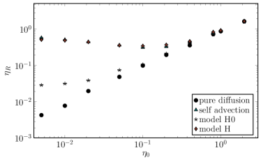
Figure 1: Renormalized viscosity as a function of the bare viscosity in four different models: 1) pure momentum diffusion (no mode-couplings), 2) self-advection ($\pi^{T}$ only couples to itself), 3) critical model H0 (mutual advection of $\phi$ and $\vec{\pi}_{T}$ only), and 4) model H at the critical point. All data were taken in lattice volume $V=L^{3}$ with $L=48$ and with $\rho=1$.

Static behavior: We first consider the static equilibrium state of the fluid described by Eqs. (1,II). The Hamiltonian does not contain any coupling between $\phi$ and $\pi_{T}$, and in the continuum, we expect the static correlation function $C(\vec{x})=\langle\phi(0,t)\phi(\vec{x},t)\rangle$ of the order parameter to be unaffected by the dynamics of the momentum density. In particular, the critical value of the mass parameter is expected to agree with the value previously determined in model A and B, $m_{c}^{2}=-2.2858$ (for $\lambda=4$)Schäfer and Skokov (2022); Chattopadhyay et al. (2023) and the correlation function $C(\vec{x})$ is predicted to be the same in model B and model H . In practice, our advection step does not conserve the potential energy of $\phi$ exactly, and we see a small shift $\delta m_{c}^{2}=-0.030$ in the critical mass parameter . After taking this shift into account, we find that the correlation function $C(\vec{x})$ is the same in models B and H Chattopadhyay et al. (2024).

Renormalization of the shear viscosity: Next we study the dynamics of the momentum density without the coupling to the order parameter $\phi$. This corresponds to the non-critical dynamics of a fluid in the limit $m^{2}\to\infty$. It was previously observed that the non-linear self-coupling of $\vec{\pi}$ leads a renormalization of the shear viscosity, referred to as the “stickiness of sound” in Kovtun et al. (2011). In the present case, the phenomenon is more accurately characterized as the stickiness of shear waves. A one-loop calculation predicts that Kovtun et al. (2011); Chafin and Schäfer (2013)

$$\eta_{R}=\eta+\frac{7}{60\pi^{2}}\frac{\rho T\Lambda}{\eta}\,,$$ (15)

where $\Lambda\simeq\pi/a$ is the UV cutoff. We have extracted the renormalized viscosity from the exponential decay of the unequal time correlation function $\langle\pi^{T}_{i}(0,\vec{k})\pi^{T}_{i}(t,-\vec{k})\rangle\sim\exp(-(\eta_{R}/\rho)k^{2}t)$ for the first non-tivial momentum mode in the cartesian direction $j$ for $i\neq j$. The result is shown in Fig. 1. We observe that as the bare viscosity is reduced, the renormalized $\eta_{R}$ levels off and then increases, in agreement with Eq. (15).

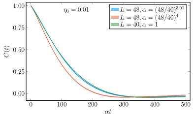
Figure 2: Dynamic order parameter correlation function $C(t,\vec{k})$ for the second non-trivial momentum mode and for different values of $L$ plotted as a function of the scaled time variable. This figure shows data taken at $\eta_{0}=10^{-2}$ for $L=40$ and $48$. Data collapse occurs for $z\simeq 3.01$, and the model B value $z=4$ is clearly excluded.

We have also studied the renormalization of $\eta$ in a theory in which the coupling between $\phi$ and $\vec{\pi}^{T}$ is retained, but the self-advection of $\vec{\pi}^{T}$ is ignored. This is a consistent truncation of model H, which we will call model H0. Indeed, the self-coupling of $\vec{\pi}^{T}$ is irrelevant in the sense of the renormalization group (RG), and model H0 is sufficient to compute critical exponents for the liquid-gas critical endpoint Hohenberg and Halperin (1977). In model H0 critical fluctuations lead to a multiplicative renormalization

$$\eta_{R}=\eta\left[1+\frac{8}{15\pi^{2}}\log(\xi/\xi_{0})\right],$$ (16)

where $\xi$ is the correlation length and $\xi_{0}\simeq a$ is the bare correlation length. This effect is difficult to observe because of the small prefactor in Eq. (16). Non-critical fluctuations generate a finite additive renormalization, $\eta_{R}=(T\xi_{0})/(160\pi\Gamma)$. This effect is also much smaller compared to Eq. (15). Indeed, Fig. 1 shows that the renormalized viscosity in model H0 continues to drop with $\eta$ and can reach very small values of order $\eta_{R}\simeq 10^{-2}$.

Dynamical scaling: Consider the time-dependent correlation function $C(\vec{k},t)=\langle\phi(\vec{k},0)\phi(-\vec{k},t)\rangle$. Dynamical scaling is the hypothesis that $\tilde{C}(k\xi,t/\xi^{z})$, where $z$ is called the dynamical exponent, is a universal function near the critical point. To understand the behavior of the correlation function it is useful to start from the prediction of the mode coupling theory Hohenberg and Halperin (1977). In this approximation, it is assumed that the correlation function is controlled by a single relaxation rate, $C(\vec{k},t)\sim\exp(-\Gamma_{k}t)$, and that the renormalized viscosity $\eta_{R}$ is a constant, independent of $\xi$. Based on these assumptions one finds

$$\Gamma_{k}=\frac{\Gamma}{\xi^{4}}\left(k\xi\right)^{2}\left(1+(k\xi)^{2}\right)+\frac{T}{6\pi\eta_{R}\xi^{3}}K(k\xi)\,,$$ (17)

where the Kawasaki function $K(x)$ is given by $K(x)\simeq x^{2}$ for $x\ll 1$ and $K(x)\simeq(3\pi/8)x^{3}$ for $x\gg 1$ Kawasaki (1970). This result suggests that the dynamic exponent crosses over from $z\simeq 4$ at modest values of the correlation length to $z\simeq 3$ if the correlation length is large, $\xi\gg(6\pi\eta_{R}\Gamma)/T$.

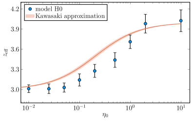
Figure 3: Scaling exponent $z$ extracted from the dynamic correlation functions for different values of the bare viscosity $\eta_{0}$ in model H0. We determined $z$ by comparing the correlation function for two different volumes, $L=40$ and $48$. We also show the prediction of the Kawasaki approximation, equ. (17); the error band is defined by varying the correlation length in the range $\xi\in[L/2\pi,L/2]$.

The values $z=3$ and $4$ are approximate, a more sophisticated calculation using the $\epsilon$-expansion gives $z=3.07$ and $z=3.96$, but the Kawasaki function is a very good approximation to the behavior of real fluids Swinney and Henry (1973). We conclude from Eq. (17) that in any finite volume, we are likely to observe a scaling exponent between 3 and 4, and that observing the model H scaling exponent requires a combination of a very large correlation length and a small viscosity.

Since the renormalized viscosity is smaller in model H0 (see Fig. 1) we have explored the scaling behavior in model H0. At the critical point $m^{2}=m_{c}^{2}$ we compute the correlation for a range of values of $\eta$ and $L^{3}$. For any given $\eta$ we look for data collapse when comparing different $L$ in order to determine the value of $z$. This is shown in Fig. 2 for $\eta=0.01$ and $L=40$ and $L=48$. We observe that scaling works very well. We then plot the extracted value of $z$ as a function of $\eta$. The result is shown in Fig. 3, and compared to the Kawasaki prediction. We observe the expected crossover from $z\simeq 4$ at large viscosity to $z\simeq 3$ for small viscosity. For $\eta=10^{-2}$ we obtain the dynamical exponent $z\simeq 3.013\pm 0.058$, consistent with the prediction of the two-loop $\epsilon$-expansion, $z\simeq 3.0712$ Adzhemyan et al. (1999).

Non-Gaussian moments: Having established that our numerical results are compatible with theoretical expectations, we turn to an observable that is not easily predicted by approximate analytical methods. Consider the correlation function of higher moments of the order parameter

$$G_{n}(t)=\langle M^{n}(t)M^{n}(0)\rangle\,,\hskip 7.11317ptM(t)=\int_{V}d^{3}x\,\phi(\vec{x},t)\,,$$ (18)

where $V$ is a sub-volume of the simulation volume. Higher cumulants of the order parameter have been proposed as signatures of critical behavior Stephanov (2009), and their time evolution was previously studied in Mukherjee et al. (2015); An et al. (2023); Schäfer and Skokov (2022).

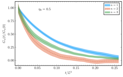
Figure 4: Correlation functions $G_{n}(t)=\langle M^{n}(t)M^{n}(0)\rangle$ in model H at the critical point for physical values of the parameters (see text). The calculation was performed for $L=48$ with $M$ integrated over half of the volume. For even $n$ we subtract disconnected pieces.

We consider model H with parameters relevant to a QCD critical endpoint. We take $a=0.75$ fm and $\Delta t=0.3$ fm, and consider a temperature $T=130$ MeV. Then, the enthalpy density of a non-interacting quark-gluon plasma corresponds to $\rho=11.1$ in lattice units. A viscosity to entropy density ratio $\eta/s=1/(4\pi)$ implies $\eta=0.50$ . We take a simulation volume $V_{0}=L^{3}$ and measure the order parameter in half the simulation volume. The results are shown in Fig. 4. The correlation functions satisfy dynamical scaling for all values of $n$, but the relaxation time depends on $n$. In particular, $G_{2}(t)$ decays more quickly than $G_{1}(t)$, but the relaxation rate of $G_{3}(t)$ is intermediate between $G_{1}(t)$ and $G_{2}(t)$. These results are not compatible with simple mean field models. Note that at the critical point the correlation length is only limited by $L$, and equilibration is extremely slow: In physical units, the $1/e$ decay time in Fig. 4 exceeds $10^{3}$ fm.

V Summary and outlook:

In this work we have presented a method for performing stochastic fluid dynamics simulations. We find that the dynamic scaling exponent in a near-critical fluid depends sensitively on the value of the correlation length and the shear viscosity. Genuine Model H behavior with $z\simeq 3$ requires a large correlation length and small shear viscosity. We also observe that while the self-coupling of the momentum density is technically irrelevant in the sense of the renormalization group (the critical behavior of model H and H0 is the same) it is numerically quite important in limiting how small the viscosity can become.

There are a number of important future directions that we wish to pursue. One important goal is to study realistic backgrounds, corresponding to an expanding and cooling fluid. There are two basic approaches that one might follow. One approach is to extend the methods described in this work to stochastic relativistic fluid dynamics, where we retain all the degrees of freedom of the fluid (both shear and sound modes). This could be accomplished along the lines recently proposed in Basar et al. (2024). Another option is to couple the model described here to a deterministic background flow, obtained from conventional fluid dynamic simulations.

Acknowledgments: This work is supported by the U.S. Department of Energy, Office of Science, Office of Nuclear Physics through the Contracts DE-FG02-03ER41260 (T.S.) and DE-SC0020081 (V.S.). We used computing resources provided by the North Carolina State University High Performance Computing Services Core Facility (RRID:SCR-022168), as well as resources funded by the Wesley O. Doggett endowment. We thank Andrew Petersen for assistance in working with the NCSU HPC infrastructure.

References

- Aoki et al. (2006) Y. Aoki, G. Endrodi, Z. Fodor, S. D. Katz, and K. K. Szabo, Nature 443, 675 (2006), arXiv:hep-lat/0611014 .
- Stephanov et al. (1998) M. A. Stephanov, K. Rajagopal, and E. V. Shuryak, Phys. Rev. Lett. 81, 4816 (1998), arXiv:hep-ph/9806219 .
- Bzdak et al. (2020) A. Bzdak, S. Esumi, V. Koch, J. Liao, M. Stephanov, and N. Xu, Phys. Rept. 853, 1 (2020), arXiv:1906.00936 [nucl-th] .
- Bluhm et al. (2020) M. Bluhm et al., Nucl. Phys. A 1003, 122016 (2020), arXiv:2001.08831 [nucl-th] .
- An et al. (2022) X. An et al., Nucl. Phys. A 1017, 122343 (2022), arXiv:2108.13867 [nucl-th] .
- Adam et al. (2021) J. Adam et al. (STAR), Phys. Rev. Lett. 126, 092301 (2021), arXiv:2001.02852 [nucl-ex] .
- Rajagopal and Wilczek (1993) K. Rajagopal and F. Wilczek, Nucl. Phys. B 399, 395 (1993), arXiv:hep-ph/9210253 .
- Berdnikov and Rajagopal (2000) B. Berdnikov and K. Rajagopal, Phys. Rev. D 61, 105017 (2000), arXiv:hep-ph/9912274 .
- Son and Stephanov (2004) D. T. Son and M. A. Stephanov, Phys. Rev. D 70, 056001 (2004), arXiv:hep-ph/0401052 .
- Hohenberg and Halperin (1977) P. C. Hohenberg and B. I. Halperin, Rev. Mod. Phys. 49, 435 (1977).
- Schweitzer et al. (2020) D. Schweitzer, S. Schlichting, and L. von Smekal, Nucl. Phys. B 960, 115165 (2020), arXiv:2007.03374 [hep-lat] .
- Schäfer and Skokov (2022) T. Schäfer and V. Skokov, Phys. Rev. D 106, 014006 (2022), arXiv:2204.02433 [nucl-th] .
- Nahrgang et al. (2019) M. Nahrgang, M. Bluhm, T. Schäfer, and S. A. Bass, Phys. Rev. D 99, 116015 (2019), arXiv:1804.05728 [nucl-th] .
- Schweitzer et al. (2022) D. Schweitzer, S. Schlichting, and L. von Smekal, Nucl. Phys. B 984, 115944 (2022), arXiv:2110.01696 [hep-lat] .
- Mukherjee et al. (2015) S. Mukherjee, R. Venugopalan, and Y. Yin, Phys. Rev. C 92, 034912 (2015), arXiv:1506.00645 [hep-ph] .
- Akamatsu et al. (2017) Y. Akamatsu, A. Mazeliauskas, and D. Teaney, Phys. Rev. C 95, 014909 (2017), arXiv:1606.07742 [nucl-th] .
- Stephanov and Yin (2018) M. Stephanov and Y. Yin, Phys. Rev. D 98, 036006 (2018), arXiv:1712.10305 [nucl-th] .
- Martinez and Schäfer (2019) M. Martinez and T. Schäfer, Phys. Rev. C 99, 054902 (2019), arXiv:1812.05279 [hep-th] .
- Akamatsu et al. (2019) Y. Akamatsu, D. Teaney, F. Yan, and Y. Yin, Phys. Rev. C 100, 044901 (2019), arXiv:1811.05081 [nucl-th] .
- An et al. (2019) X. An, G. Başar, M. Stephanov, and H.-U. Yee, Phys. Rev. C 100, 024910 (2019), arXiv:1902.09517 [hep-th] .
- An et al. (2020) X. An, G. Başar, M. Stephanov, and H.-U. Yee, Phys. Rev. C 102, 034901 (2020), arXiv:1912.13456 [hep-th] .
- An et al. (2021) X. An, G. Başar, M. Stephanov, and H.-U. Yee, Phys. Rev. Lett. 127, 072301 (2021), arXiv:2009.10742 [hep-th] .
- Berges et al. (2010) J. Berges, S. Schlichting, and D. Sexty, Nucl. Phys. B 832, 228 (2010), arXiv:0912.3135 [hep-lat] .
- Pihan et al. (2023) G. Pihan, M. Bluhm, M. Kitazawa, T. Sami, and M. Nahrgang, Phys. Rev. C 107, 014908 (2023), arXiv:2205.12834 [nucl-th] .
- Florio et al. (2022) A. Florio, E. Grossi, A. Soloviev, and D. Teaney, Phys. Rev. D 105, 054512 (2022), arXiv:2111.03640 [hep-lat] .
- Chattopadhyay et al. (2023) C. Chattopadhyay, J. Ott, T. Schäfer, and V. Skokov, Phys. Rev. D 108, 074004 (2023), arXiv:2304.07279 [nucl-th] .
- Florio et al. (2023) A. Florio, E. Grossi, and D. Teaney, (2023), arXiv:2306.06887 [hep-lat] .
- Folk and Moser (2006) R. Folk and H.-G. Moser, J. Phys. A 39, R207 (2006).
- An et al. (2023) X. An, G. Basar, M. Stephanov, and H.-U. Yee, Phys. Rev. C 108, 034910 (2023), arXiv:2212.14029 [hep-th] .
- Parotto et al. (2020) P. Parotto, M. Bluhm, D. Mroczek, M. Nahrgang, J. Noronha-Hostler, K. Rajagopal, C. Ratti, T. Schäfer, and M. Stephanov, Phys. Rev. C 101, 034901 (2020), arXiv:1805.05249 [hep-ph] .
- Kahangirwe et al. (2024) M. Kahangirwe, S. A. Bass, E. Bratkovskaya, J. Jahan, P. Moreau, P. Parotto, D. Price, C. Ratti, O. Soloveva, and M. Stephanov, (2024), arXiv:2402.08636 [nucl-th] .
- Martinez et al. (2019) M. Martinez, T. Schäfer, and V. Skokov, Phys. Rev. D 100, 074017 (2019), arXiv:1906.11306 [hep-ph] .
- Morinishi et al. (1998) Y. Morinishi, T. Lund, O. Vasilyev, and P. Moin, Journal of Computational Physics 143, 90 (1998).
- Chattopadhyay et al. (2024) C. Chattopadhyay, J. Ott, T. Schäfer, and V. Skokov, (2024), in preparation.
- Shu and Osher (1988) C.-W. Shu and S. Osher, Journal of computational physics 77, 439 (1988).
- Kovtun et al. (2011) P. Kovtun, G. D. Moore, and P. Romatschke, Phys. Rev. D 84, 025006 (2011), arXiv:1104.1586 [hep-ph] .
- Chafin and Schäfer (2013) C. Chafin and T. Schäfer, Phys. Rev. A 87, 023629 (2013), arXiv:1209.1006 [cond-mat.quant-gas] .
- Kawasaki (1970) K. Kawasaki, Annals of Physics 61, 1 (1970).
- Swinney and Henry (1973) H. L. Swinney and D. L. Henry, Phys. Rev. A 8, 2586 (1973).
- Adzhemyan et al. (1999) L. T. Adzhemyan, A. Vasiliev, Y. S. Kabrits, and M. V. Kompaniets, Theoretical and Mathematical Physics 119, 454 (1999).
- Stephanov (2009) M. A. Stephanov, Phys. Rev. Lett. 102, 032301 (2009), arXiv:0809.3450 [hep-ph] .
- Basar et al. (2024) G. Basar, J. Bhambure, R. Singh, and D. Teaney, (2024), arXiv:2403.04185 [nucl-th] .