Cosmic Inflation: Background dynamics,
Quantum fluctuations and Reheating

Abstract

Cosmic inflation is a transient period of rapid accelerated expansion of space which has been hypothesized to have taken place prior to the hot Big Bang phase of the universe. It is the leading paradigm of the very early universe that provides natural initial conditions for the hot Big Bang phase, both at the background and at the perturbation level. In fact, quantum vacuum fluctuations during inflation generate both scalar and tensor type primordial perturbations that are correlated over super-Hubble scales. The scalar fluctuations, upon their Hubble-entry, lead to the temperature and density inhomogeneities in the primordial plasma which eventually grow via gravitational instability to form the large-scale structure of the universe. Furthermore, the inflationary tensor fluctuations constitute a background of stochastic Gravitational Waves (GWs) upon their Hubble-entry in the post-inflationary universe. The correlation functions of inflationary fluctuations constitute the primary observational tool to probe the high energy physics of the early universe.

Furthermore, in the inflationary paradigm all constituents of the universe at the subsequent radiation-dominated epoch were created during a process known as reheating, which is supposed to have taken place after the end of inflation. In the simplest inflationary scenario, the energy density of the universe was concentrated in a slowly evolving scalar field, called the inflaton. After the end of inflation, the (almost) homogeneous inflaton condensate started to oscillate coherently around the minimum of its effective potential. The oscillating inflaton condensate then decayed and transferred all of its energy to the quanta of other fields that are coupled to the inflaton. Subsequently, the universe became thermalized at some high temperature, marking the commencement of the hot Big Bang phase. Since reheating is the intermediate stage between inflation and the radiation-dominated hot Big Bang phase, it is associated with a number of important aspects of the hot Big Bang cosmology.

In these lecture notes, we provide a pedagogical introduction to some aspects of the inflationary cosmology including the background scalar field dynamics, generation of primordial seed perturbations via quantum fluctuations during inflation, and the process of reheating after inflation in the single-field inflationary paradigm.

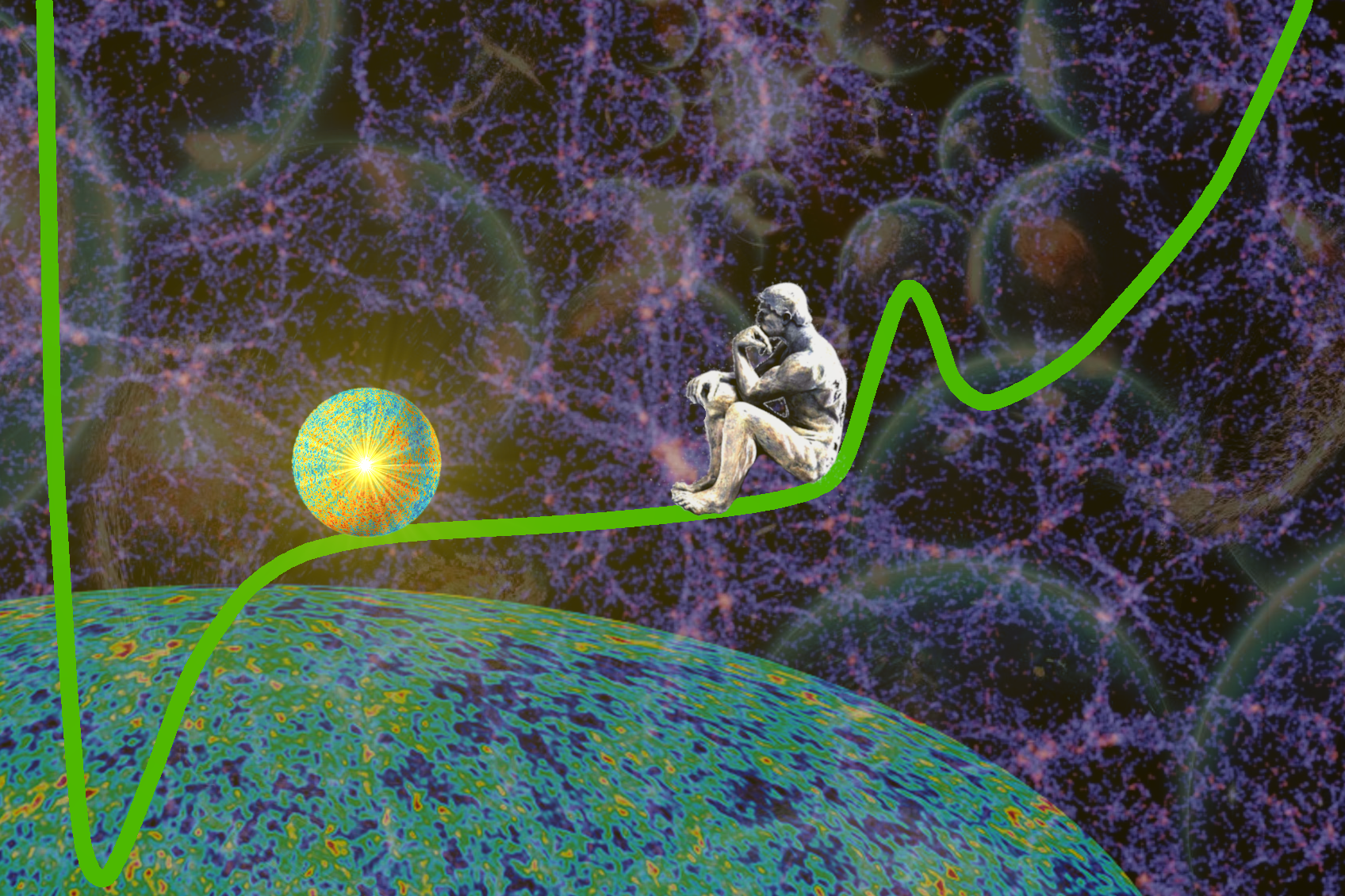
Figure 1: [NASA/ESA, WMAP, PLANCK teams, Max Planck Institute for Astrophysics, Auguste Rodin.]

Introductory Lecture Notes

Declaration

These are introductory lecture notes primarily based on a set of lectures I delivered as a supplementary course in Cosmology for the PhD coursework at IUCAA (India) in Jan/Feb 2024. Presentation of some of the topics originated from my lectures for the Master students I supervised in between 2017-23. The lectures are primarily intended for PhD students who have had introductory courses on general relativity, quantum field theory, particle physics and cosmology. I have made an attempt to compose a range of topics that are somewhat complementary to many of the existing (excellent) lecture notes in the literature and consequently, a number of key aspects of the inflationary cosmology have not been included in the present version. The approach here is relatively pedagogical and various concepts are presented from a personal perspective. Some topics are covered quite comprehensively, and hence I hope these notes will also be useful to researchers in the field. The present version may quite possibly contain typos and errors. I would be grateful to receive comments, suggestions, and typo corrections via email.

– Richard P. Feynman

1 Introduction

Remarkable theoretical and observational advancements in cosmology over the past five decades have led to the emergence of the standard paradigm of the universe, popularly known as the Big Bang Theory, within which the spatially flat ${\rm\Lambda}$CDM model is often used as the fiducial/concordance model. This standard paradigm of cosmology describes the evolution of the universe reasonably well, starting from about 1 sec after the Big Bang, all the way until the present epoch.

However, the success of the concordance model relies upon the existence of hitherto unknown matter and energy constituents in the universe, in particular, a non-baryonic dark matter component that reinforces the formation of the large scale structure (LSS) of the universe in the matter-dominated (MD) epoch, as well as a negative pressure dark energy component responsible for the observed accelerated expansion of space closer to the present epoch. In the concordance model, the dark matter is often assumed to be cold and pressureless on cosmological scales, and dark energy is assumed to be the cosmological constant $\Lambda$. The nature of dark matter and dark energy are two of the greatest puzzles confronting the standard cosmological paradigm in the $21^{\rm st}$ century.

On the other hand, the success of the standard paradigm also heavily relies upon the specific primordial initial conditions at the beginning of the hot Big Bang phase. At the background level, these initial conditions take the form of (i) extreme spatial flatness of the universe throughout its evolution history and (ii) high degree of spatial homogeneity and isotropy over large length scales in the early universe. In particular, the average temperature of the Cosmic Microwave Background (CMB) seems to be uniform up to a high degree of precision across all sky. Since the standard Big Bang theory assumes that the universe was born in the state of being radiation dominated (RD) with decelerated expansion, both of the aforementioned initial conditions are highly non-trivial (unnatural) and appear to be extremely fine tuned. More importantly, we have also established the existence of tiny primordial curvature fluctuations in the early universe (via temperature and polarisation fluctuations in the CMB over a range of angular scales) which seed the formation of the large-scale structure in the late universe via gravitational instability. The latest CMB observations by the Planck collaboration [1, 2] indicate that the initial curvature fluctuations were highly Gaussian, nearly scale-invariant and predominantly adiabatic in nature. Consequently, these specific properties of the primordial fluctuations, combined with the extreme spatial flatness, homogeneity and isotropy strongly point towards the existence of a non-standard (neither radiation nor matter dominated) transient epoch in the very early universe prior to the commencement of the hot Big Bang phase. In an expanding universe, assuming Einstein’s theory of Gravity to hold at early times, these primordial initial conditions can be explained only if this transient period exhibited rapid accelerated expansion of space, known as ‘cosmic inflation’.

The inflationary paradigm [3, 4, 5, 6, 7, 8, 9] has emerged as the leading scenario for describing the very early universe and for setting natural initial conditions for the hot Big Bang phase. One of the key predictions of the inflationary scenario is the unavoidable quantum-mechanical production of primordial (scalar) curvature perturbations on super-Hubble scales [10, 11, 12, 13]. In fact, the inflationary predictions for the statistical properties of these scalar quantum fluctuations (made in the early 1980s) match extremely well with the latest precision CMB observations by the Planck collaboration (data released in 2018) over a range of length scales, which consolidates inflation as a feasible scenario of the pre-hot Big Bang universe [14, 1, 2, 15, 16]. In its simplest realization, inflation is usually assumed to be sourced by a single canonical scalar field $\varphi$ with a shallow self-interaction potential $V(\varphi)$ which is minimally coupled to gravity [8, 9, 17]. At early times, when the inflaton is higher up in its potential, the universe inflates nearly exponentially. While, towards the end of inflation, the inflaton begins to roll rapidly down its potential before exhibiting coherent oscillations around its minimum.

Another crucial prediction of inflation is the generation of tensor perturbations via quantum fluctuations of the transverse and traceless part of the metric tensor during the accelerated expansion, which constitute a stochastic background of relic gravitational waves (GWs) [18, 19, 20]. Scalar and tensor perturbations generated during inflation create distinctive imprints on the primordial CMB radiation which can be used to deduce the scalar spectral index $n_{{}_{S}}$ and the tensor-to-scalar ratio $r$ – two of the most important observables which can be used to rule out competing inflationary models [21, 17, 1, 2].

It is well known that the inflationary GW power spectrum at large scales provides us with important information about the nature of an inflaton field due to its direct relation to the inflaton potential [19, 22]. Of greater importance is the fact that their spectrum, $\Omega_{{}_{\rm GW}}(f)$ (defined as the fractional energy density of GWs per logarithm interval of their frequency $f$ at the present epoch) and the spectral index $n_{{}_{\rm GW}}={\rm d}\ln{\Omega_{{}_{\rm GW}}}/{\rm d}\ln{f}$ at sufficiently small scales can serve as key probes to the high energy physics of the post-inflationary primordial epoch. The primordial spectrum of relic gravitational radiation at small scales is exceedingly sensitive to the post-inflationary primordial equation of state (EoS), $w$. In fact, the GW spectrum has distinctly different properties for stiff/soft equations of state. For a stiff EoS, $w>1/3$, the GW spectrum shows a blue tilt: $n_{{}_{\rm GW}}>0$, that increases the GW amplitude on small scales. A softer EoS, $w<1/3$, on the other hand, leads to a red tilt, whereas the radiation EoS, $w=1/3$, results in a flat spectrum with $n_{{}_{\rm GW}}\simeq 0$.

Another key aspect of inflationary cosmology is the epoch of reheating during which the energy stored in the inflaton is transferred into the radiative degrees of freedom of the hot Big Bang phase. The post-inflationary history of the universe, prior to the commencement of Big Bang Nucleosynthesis (BBN), remains observationally inaccessible at present, despite a profusion of theoretical progress [23, 24, 25, 26, 27, 28, 29, 30, 31] in this direction. It is expected, however, that the post-inflationary universe in between the end of inflation and the beginning of the radiation domination phase passed through a series of physical epochs [32], each of which can be characterized by an EoS, $w_{i}$. Potential relics from this primordial epoch in the form of primordial black holes, oscillons and gravitational waves will provide us with key information about the dynamics of reheating in the upcoming decades.

In the following, we will provide a pedagogical introduction to the inflationary dynamics. After a brief review of the standard cosmological paradigm in Sec. 2, we will provide a discussion of the initial conditions for the early universe in Sec. 3 and demonstrate that, in the standard radiation-dominated universe, the initial conditions need to be highly fine-tuned. Then we will discuss the proposal of the inflationary scenario in the pre-hot Big Bang epoch to address the background initial conditions in Sec. 4. Sec. 5 is dedicated to the background scalar field dynamics during inflation. In Sec. 6, we will then turn our attention to the most important predictions of the inflationary hypothesis: the generation of scalar and tensor fluctuations that are correlated over super-Hubble scales. Sec. 7 is devoted to a discussion on the latest observational constraints on inflation, while the post-inflationary reheating dynamics is introduced in Sec. 8. We will provide a discussion of some of the key aspects of inflationary cosmology that have not been considered in detail in these notes in Sec. 9 and conclude by providing references to supplementary material on inflation in Sec. 10.

Various appendices provide more technical as well as supplementary information on the subject. Apps. A and B discuss the thermal history and post-inflationary kinematics of the universe, respectively. App. C provides a discussion on the Hamilton-Jacobi formalism, with an application to the power-law inflation. Apps. D, E and F are dedicated to the analytical treatment of fluctuations in the inflationary and de Sitter spacetimes.

2 Standard cosmological model: a brief review

As discussed in the introductory section, the observable universe appears to be spatially flat, homogeneous, and isotropic on large cosmological scales throughout its probed history, as inferred from the LSS and CMB observations as well as BBN constraints. The space-time metric of a nearly homogeneous and isotropic universe exhibits (approximate) spatial translation and rotation isometries and hence, is represented by the Friedmann-Lemaître-Robertson-Walker (FLRW) metric which takes the form

$${\rm d}s^{2}=-{\rm d}t^{2}+a^{2}(t)\,\left[\frac{{\rm d}r^{2}}{1-K\,r^{2}}+r^{2}\,{\rm d}\theta^{2}+r^{2}\,\sin^{2}{\theta}\,{\rm d}\phi^{2}\right]\,;$$ (1)

where $K=0,\,\pm 1$ characterizes the uniform curvature of constant-time spatial hypersurface. $K=0$ corresponds to a spatially flat $\mathbb{R}^{(3)}$ universe, $K=1$ (positive spatial curvature) corresponds to a spatially closed $\mathbb{S}^{(3)}$ universe and $K=-1$ (negative spatial curvature) corresponds to a spatially open hyperbolic $\mathbb{H}^{(3)}$ universe, see Refs. [24, 33, 34, 35]. Specializing to the spatially flat FLRW metric for which $K=0$, we get

$${\rm d}s^{2}=-{\rm d}t^{2}+a^{2}(t)\,\delta_{ij}\,{\rm d}x^{i}{\rm d}x^{j}\,.$$ (2)

The rate of spatial expansion is described by the Hubble parameter which is defined as

$$H=\frac{\dot{a}}{a}\,.$$ (3)

Expansion of the universe results in redshifting of the wavelength (or decreasing of the momentum along the geodesics) of massless particles such as photons. The redshift is related to the scale factor via

$$1+z=\frac{a_{0}}{a}\,,$$ (4)

where $a_{0}$ is the present day scale factor for which $z=0$. We will not discuss the kinematics of FLRW space-time and refer the interested readers to standard textbooks on the subject, for example Ref. [35].

Dynamics of space-time, sufficiently below the Planck scale, is governed by the Einstein’s Field Equations

$$G_{\mu\nu}\equiv R_{\mu\nu}-\frac{R}{2}\,g_{\mu\nu}=\frac{1}{m_{p}^{2}}\,T_{\mu\nu}\,.$$ (5)

For a homogeneous and isotropic distribution of matter-energy constituents described by the energy-momentum tensor $T^{\mu}_{\;\>\;\nu}\equiv\mathrm{diag}\left(-\rho,\,p,\,p,\,p\right)$, and the metric represented by the FLRW line element given in Eq. (1), the time-time and space-space components of Einstein’s field equations take the form

$$H^{2} = \frac{1}{3{m_{p}^{2}}}\,\rho-\frac{K}{a^{2}}\,,$$ (6)

$$\frac{\ddot{a}}{a} \equiv \dot{H}+H^{2}=-\frac{1}{6{m_{p}^{2}}}\,(\rho+3\,p)\,.$$ (7)

$\rho$ and $p$ are energy density and pressure respectively. Eqs. (6) and (7) are called the Friedmann equations. Eq. (7) determines whether the expansion of the universe decelerates or accelerates, given the energy density and pressure of the constituents. Energy-momentum conservation leads to

$$\dot{\rho}+3\,H\,\left(\rho+p\right)=0\,,$$ (8)

which can also be derived by combining Eqs. (6) and (7). In cosmology, we will often work with perfect fluids for which the pressure and density will be related via an equation of state (EoS) of the form

$$p=w\,\rho\,,$$ (9)

where the equation of state parameter $w\in\left[-1,\,1\right]$. Consequently, we can write Eq. (8) as

$$\dot{\rho}+3\,H\,\left(1+w\right)\rho=0\,,$$ (10)

whose general solution for constant $w$ can be written as

$$\rho(a)=\rho_{1}\,\left(\frac{a}{a_{1}}\right)^{-3(1+w)}\,,$$ (11)

where $\rho_{1}$ is the energy density at some reference epoch $a_{1}$ which is usually taken to be the scale factor of the present epoch. Incorporating the above expression into Eq. (6), we obtain

$$a(t)=a_{1}\,\left(\frac{t}{t_{1}}\right)^{\frac{2}{3(1+w)}}\,;\quad H(a)=H_{1}\,\left(\frac{a}{a_{1}}\right)^{-3(1+w)/2}\,.$$ (12)

Note that the EoS parameter for radiation (relativistic constituents), matter (non-relativistic constituents), and a cosmological constant are given by $w_{r}=\frac{1}{3}$, $w_{m}\simeq 0$, and $w_{\rm DE}=-1$ respectively, which leads to the following expressions for the energy density

$$\rho(a)\propto\begin{cases}1/a^{4}\,;&{\rm RD}\\ 1/a^{3}\,;&{\rm MD}\,;\\ {\rm const.}\,&{\rm CCD}\,,\end{cases}$$ (13)

and the following expressions for scale factor in a spatially flat universe

$$a(t)\propto\begin{cases}t^{1/2}\,;&{\rm RD}\\ t^{2/3}\,;&{\rm MD}\,;\\ e^{H\,t}\,&{\rm CCD}\,.\end{cases}$$ (14)

A pure cosmological constant-dominated (CCD) universe is called the ‘de Sitter’ (dS) universe for which the Hubble parameter $H$ is constant and the scale factor expands exponentially. In general, the universe can be filled with a number of different constituents at a given time (which is the case for our own universe). We assume that different constituents with densities $\rho_{i}$, and EoS parameters $w_{i}$, do not interact with each other (apart from gravity). Then the Friedmann Eqs. (6), (7) and energy momentum conservation Eq. (8) take the form

$$H^{2} = \frac{1}{3{m_{p}^{2}}}\,\sum_{i}\,\rho_{i}-\frac{K}{a^{2}}\,,$$ (15)

$$\frac{\ddot{a}}{a} \equiv \dot{H}+H^{2}=-\frac{1}{6{m_{p}^{2}}}\,\sum_{i}\,\left(1+3\,w_{i}\right)\,\rho_{i}\,,$$ (16)

$$\dot{\rho_{i}} = -3\,H\,\left(1+w_{i}\right)\rho_{i}\,,$$ (17)

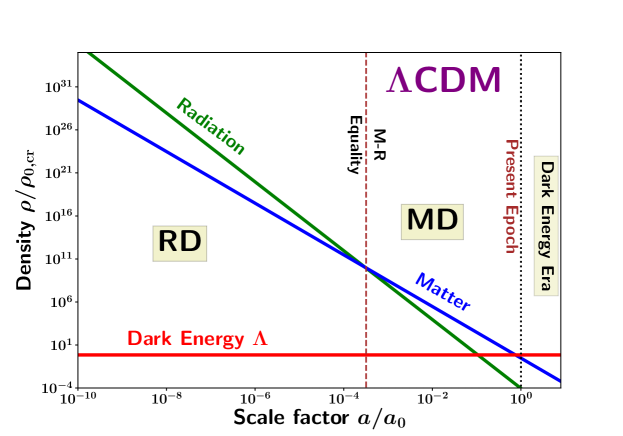
Figure 2: The evolution of the density of radiation, matter and dark energy in the context of the flat $\Lambda$CDM concordance cosmology. Note that, while the density of the matter and radiative degrees of freedom (represented by the solid blue and green curves respectively) evolve with time, the density of the cosmological constant $\Lambda$ (represented by the solid red curve) remains constant.

A range of cosmological and astrophysical observations relevant to the standard cosmological paradigm indicate that our universe was radiation dominated at early times during the hot Big Bang plasma phase. It made a transition to the matter dominated epoch around a redshift $z\simeq 3400$, while continuing to exhibit a decelerated expansion throughout most of its expansion history. However, more recently around the redshift $z\sim 0.7$ the expansion of the universe started accelerating closer to the present epoch. A cosmological constant $\Lambda$ with $w_{\rm DE}=-1$ explains most cosmological observations very well. All the stable constituents of the Standard Model of particle physics account for the radiation and baryon fraction of the energy budget of our universe. While pressureless cold dark matter (CDM) and a small positive cosmological constant ($\Lambda$) as the dark energy constitute the dominant energy budget of the universe at the present epoch. This is often referred to as the standard or concordance model of cosmology, fittingly known as the flat $\Lambda$CDM model.

It is convenient to introduce dimensionless density parameters $\Omega_{i}$ which are defined as

$$\Omega_{i}=\frac{\rho_{i}}{\rho_{c}}\,;\quad{\rm with}\quad\rho_{c}=3\,m_{p}^{2}\,H^{2}$$ (18)

being the critical energy density. Hence the Hubble parameter for the flat ${\rm\Lambda}$CDM model can be written as

$$H=H_{0}\,\sqrt{\Omega_{0r}\left(a_{0}/a\right)^{4}+\Omega_{0m}\left(a_{0}/a\right)^{3}+\Omega_{0\Lambda}}=H_{0}\,\sqrt{\Omega_{0r}\left(1+z\right)^{4}+\Omega_{0m}\left(1+z\right)^{3}+\Omega_{0\Lambda}}\,,$$ (19)

where $\Omega_{0i}$ is the dimensionless density parameter of a constituent at the present epoch. Note that, in a spatially flat universe,

$$\sum_{i}\Omega_{i}(a)=1$$

at all cosmological epochs. The latest CMB observations reported in Ref. [1] suggest that

$$\Omega_{0r}\simeq 9.1\times 10^{-5}\,;\leavevmode\nobreak\ \Omega_{0m}\simeq 0.315\,;\leavevmode\nobreak\ \Omega_{0\Lambda}\simeq 0.685\,.$$ (20)

The expression for the Hubble parameter in Eq. (19) is accurate until about $z\simeq 10^{9}$. At higher redshifts deep inside the radiation dominated epoch the effective number of relativistic degrees of freedom changes, implying there will be corrections to the expression for the Hubble parameter (see App. A). (This is also true for the Standard Model neutrinos, some of which are known to be massive, and hence, represent part of the non-relativistic matter at the present epoch, although they were relativistic (radiation-like) in the early universe.)

In short, the broad outline of our knowledge of modern cosmology can be succinctly summarised as follows:

• The universe is roughly homogeneous and isotropic on large cosmological length scales ($>100\leavevmode\nobreak\ {\rm Mpc}$) and exhibits negligible spatial curvature throughout its (known/probed) expansion history.

• The universe has been expanding for the last 13.8 billion years, at least from the time when it was about $1$ second old until the present epoch. The metric of the universe, at the background level, is well approximated by the flat Friedmann-Lemaître-Robertson-Walker (FLRW) line element given in Eq. (2).

• Observations of the Cosmic Microwave Background (CMB) radiation indicate that prior to the epoch when our universe was about $370,000$ years old, corresponding to a redshift of $z\simeq 1100$, it was in a thermal hot dense plasma state.

• The early universe was thermal and radiation dominated, historically termed as the hot Big Bang phase, which made a transition to the matter dominated epoch when it was around $50,000$ years old, at a redshift $z_{\rm eq}\simeq 3400$. The expansion of the universe was decelerating during both the aforementioned epochs.

• More recently, the universe has entered into a phase of accelerated expansion around the time when it was about $8$ billion years old.

• In addition to baryons, photons and neutrinos, our universe also contains a gravitationally clustering non-relativistic substance known as dark matter (DM) which is pressureless (and hence ‘cold’) on large extra-galactic scales. Observations suggest that DM is non-baryonic, in the sense that it does not interact with the Standard Model constituents at low energy (apart from gravity, of course). DM plays a dominant role in facilitating the formation of large-scale structure in the universe [44, 45, 46, 47].

• Additionally, the cosmic recipe also includes a gravitationally non-clustering negative pressure substance termed as dark energy (DE) in order to fuel the late time accelerated expansion [48, 49, 50, 47, 51, 52]. The present day equation of state of the dark energy is close to that of a cosmological constant $\Lambda$ [53, 54, 55, 56, 57, 58, 59, 60, 61, 47, 62]. The concordance cosmological model is consequently termed as the flat $\Lambda$CDM model, or more colloquially as the ‘Big Bang Theory’. Evolution of the energy density of radiation, matter and dark energy are shown in Fig. 2.

• Starting with an initial spectrum of almost scale-invariant, adiabatic, Gaussian density fluctuations [1, 2] that are correlated on super-Hubble scales, the standard cosmological paradigm successfully describes the growth and formation of structure in our universe, at least on large length scales.

• The nature of these special initial conditions for the concordance cosmology, in conjunction with CMB and LSS observations, strongly point towards a transient period of rapid accelerated expansion of space, known as Cosmic Inflation, which is supposed to have happened in the very early universe [3, 4, 5, 6, 7, 8, 9] prior to the commencement of the radiative hot Big Bang phase.

Note that there is a classical singularity in the standard Big Bang theory [63] in the context of classical general relativity where $a=0$ and the spacetime curvature diverges. We use this classical singularity to set our initial time $t=0$. However, it is crucial to mention that going backwards in time, the curvature of the spacetime of the universe will approach Planckian values before hitting the singularity and hence we expect substantial modifications to Einstein’s theory due to quantum gravity effects which are supposed to remove the classical singularity. Hence the existence of the classical singularity must not to be taken literally. For all practical purposes, we will assume that the hot Big Bang phase began at some high temperature below the Planck scale (and much above $1\leavevmode\nobreak\ {\rm MeV}$ in order to ensure successful BBN), namely

$$1\leavevmode\nobreak\ {\rm MeV}\,\ll\,T_{i}^{{\rm HBB}}\,\leq\,10^{19}\leavevmode\nobreak\ {\rm GeV}\,.$$

While the standard Big Bang theory has been remarkably successful in describing the evolution of the universe [1] both at the background and at the perturbation level, its success relies heavily upon the following initial conditions at the beginning of the hot Big Bang phase:

1. High degree of spatial flatness: As mentioned before, the background metric of the universe is consistent with being spatially flat throughout the history of the universe. In the next section, we will quantify this statement and demonstrate that this leads to a high degree of fine-tuning of the initial expansion rate of the hot Big Bang universe, usually known as the flatness problem.

2. Extreme homogeneity of the initial hypersurface: The success of BBN as well as the precision observations of the CMB indicate that the early universe was spatially homogeneous and isotropic over large length scales. For example, the temperature of the CMB is almost uniform all across the sky. In the next section, we will demonstrate that the aforementioned fact leads to the so-called horizon problem.

3. Super-Hubble correlation of seed perturbations: One of the greatest discoveries in modern cosmology is the fact that the large scale structure (LSS) of the universe is formed due to the gravitational collapse of tiny initial density fluctuations in the early universe. In fact the statistical properties of these primordial seed fluctuations have been measured very accurately by CMB and LSS observations and they have three key properties [1, 64, 2].

   • Primordial fluctuations are predominantly adiabatic, which indicates that initial fluctuations in different constituents in the hot Big Bang phase were almost the same. This further points to the fact that the seed fluctuations in the early universe emerged out of the perturbations of a single field, namely the comoving curvature fluctuations $\zeta(t,\vec{x})$ which is a gauge invariant quantity (i.e. it remains invariant under the gauge transformation from one local frame to another, that connects different ways of slicing and threading spacetime into a homogeneous background part and perturbations around that background.)

   • The power spectrum of $\zeta$ is nearly scale-invariant, namely

     $${\cal P}_{\zeta}=A_{S}\left(\frac{k}{k_{*}}\right)^{n_{{}_{S}}-1}\,;\leavevmode\nobreak\ k_{*}=0.05\,{\rm Mpc}^{-1}\,$$

     with

     $$A_{S}\simeq 2\times 10^{-9}\,,\leavevmode\nobreak\ n_{{}_{S}}-1\simeq-0.035\leavevmode\nobreak\ \leavevmode\nobreak\ ({\rm small\leavevmode\nobreak\ {\color[rgb]{1,0,0}\textbf{red\leavevmode\nobreak\ tilt}}})\,.$$

   • The primordial seed fluctuations are approximately Gaussian with probability distribution function given by

     $$P[\zeta]={\cal B}\exp\left[\frac{-\zeta^{2}}{2\sigma_{\zeta}^{2}}\left(1+f_{\rm NL}\,\zeta+...\right)\right]\,,$$

     where ${\cal B}$ is a normalisation factor. The variance $\sigma_{\zeta}^{2}$ is given by

     $$\sigma_{\zeta}^{2}=\int_{-\infty}^{\infty}\,{\rm d}\zeta\leavevmode\nobreak\ \zeta^{2}\leavevmode\nobreak\ P[\zeta]\equiv\int_{k_{\rm min}}^{k_{\rm max}}\frac{{\rm d}k}{k}\leavevmode\nobreak\ {\cal P}_{\zeta}(k)\simeq 10^{-9}\,.$$

     Latest CMB and LSS observations are consistent with $f_{\rm NL}=0$ which implies that we have not found any deviation from Gaussianity so far.

   • The temperature power spectrum of the CMB on large angular scales indicates that the primordial fluctuations exhibit non-vanishing statistical correlations on super-Hubble scales.

   These specific characteristics of the seed fluctuations demand a physical mechanism to explain their origin. As we will discuss later in these notes, quantum fluctuations during the accelerated expansion in the inflationary scenario provide a natural mechanism to explain these observed properties of the primordial fluctuations.

3 Fine-tuning of initial conditions for the hot Big Bang

3.1 High degree of spatial flatness

The fine-tuning of the initial expansion rate of the universe for the hot Big Bang phase can be stated in terms of the famous flatness problem. The first Friedmann Eq. (6) for a spatially curved universe can be written as

$$|\Omega_{\rm tot}(a)-1|\equiv|\Omega_{K}(a)|=\frac{|K|}{a^{2}\,H^{2}}=(aH)^{-2}\,,$$ (21)

where $\Omega_{K}$ corresponds to the dimensionless density parameter associated with the spatial curvature. From Eq. (12), for a single component dominated universe, we have

$$\left(aH\right)^{-1}=\left(a_{i}H_{i}\right)^{-1}\,\left(\frac{a}{a_{i}}\right)^{\frac{1+3w}{2}}\,.$$ (22)

Eq. (21) can then be described more generally for a single component dominated universe as

$$|\Omega_{\rm tot}(a)-1|=|\Omega_{\rm tot}(a_{i})-1|\,\left(\frac{a}{a_{i}}\right)^{1+3w}\leavevmode\nobreak\ \propto\leavevmode\nobreak\ a^{1+3w}\,,$$ (23)

which implies

$$|\Omega_{\rm tot}(a)-1|\propto\begin{cases}a^{2}\,;&{\rm RD}\,,\\ a\,;&{\rm MD}\,.\end{cases}$$ (24)

This shows that $\Omega_{\rm tot}(a)$ continues to diverge away from $1$ in the radiation and matter-dominated epochs. Given the present day bound on $|\Omega_{\rm tot}(a_{0})-1|$ (or equivalently, on $|\Omega_{K}(a_{0})|)$ from the latest CMB observations [14],

$$|\Omega_{K}(a_{0})|\leq 10^{-2}\,,$$

combined with the fact that $|\Omega_{K}(a)|$ has been growing ever since the commencement of the hot Big Bang phase, it seems that the early universe was spatially flat up to an unnaturally high degree of precision. In order to quantify this, let us compute the bound on $|\Omega_{K}(a_{0})|$ at the beginning of Big Bang Nucleosynthesis, which corresponds to $z_{{}_{\rm BBN}}\simeq 4\times 10^{9}$.

$$|\Omega_{K}(a_{0})|\leq 10^{-2}\Rightarrow\frac{|\Omega_{K}(a_{0})|}{|\Omega_{K}(a_{\rm BBN})|}\,|\Omega_{K}(a_{\rm BBN})|\leq 10^{-2}\,,$$

which leads to

$$|\Omega_{K}(a_{\rm BBN})|\leq 6\times 10^{-18}\,.$$ (25)

Further back in time, at the grand unification (GUT) scale ($z_{{}_{\rm GUT}}\simeq 10^{29}$), the bound on the curvature parameter becomes

$$|\Omega_{K}(a_{\rm GUT})|\leq 10^{-56}\,.$$ (26)

Our universe during most of its expansion history has been dominated by radiation and matter, hence the spatial curvature according to equation (23) should be extremely high today, even though it was small at early times. But observations suggest that the spatial curvature at the present epoch is still very small which implies that the spatial curvature in very early times must have been extremely small. In fact, the simple calculation that we carried out above demonstrates that $|\Omega_{\rm tot}|$ must have been close to $1$ up to several decimal places of accuracy at the beginning of the hot Big Bang phase in the very early universe. Another way to state the fine-tuned spatial flatness is that the initial density $\rho_{i}^{\rm tot}$ of all matter-energy components of the hot Big Bang phase must have been close to the critical density $\rho_{c}=3m_{p}^{2}H^{2}$ up to several decimal places. This also implies that the initial expansion speed $\dot{a}_{i}$ must be highly fine-tuned in order for $|\Omega_{K}|$ to remain much smaller than unity at the present epoch. Such extreme fine-tuning of the initial expansion speed is known as the flatness problem and suggests an early epoch of expansion prior to the hot Big Bang phase which can dynamically drive $\Omega_{K}$ towards an extremely small value by the time the hot Big Bang phase commences.

Note that if $K=0$ exactly, then there is no flatness problem classically. However, $K=0$ corresponds to a spatially flat universe which is either infinite in extent or has a non-trivial topology. Additionally, if the universe began around the Planck scale, then large quantum gravitational fluctuations might alter the geometry/topology of spatial hypersurfaces. Furthermore, in quantum cosmology, quantum creation of the universe usually renders it to be either positively curved [65, 66, 67] or negatively curved [68, 69].

3.2 Horizon problem

CMB observations indicate that the temperature of the early universe, closer to recombination, is almost uniform across diametrically opposite points in the sky (with very tiny variations in the temperature of CMB of the order $\Delta T/T\simeq 10^{-5}$). This suggests that the early universe was incredibly uniform over large distance scales. However, this observation leads to a potential problem in the standard hot Big Bang theory, which originates from the fact that light could have travelled only a finite distance from the beginning of the hot Big Bang phase until the emission of CMB photons around the epoch of recombination. Additionally, the spatial hypersurface at the epoch of BBN is also supposed to be highly uniform and hence the same arguments may be extrapolated to even earlier epochs. To illustrate this point explicitly, let us define the physical size of the causal horizon in cosmology.

The physical size of the causal horizon (also called the particle horizon) at any epoch $a(t)$ is defined as the maximum distance that any signal could have travelled from the beginning of the universe at $t=t_{i}$ until that epoch, and is given by

$$d_{H}(t)=a(t)\,r_{H}(t)\,.$$ (27)

Where the comoving causal horizon $r_{H}(t)$ can be computed by noting that signals propagate radially in an FLRW universe, so we have ${\rm d}\theta={\rm d}\phi=0$. Additionally, for the propagation of light (or any other massless particle), ${\rm d}s^{2}=0$ in Eq. (2), which leads to

$${\rm d}r=\frac{{\rm d}t}{a(t)}\,,$$

and hence the expression for the physical size of the causal horizon becomes

$$d_{H}(t)\equiv a(t)\,\int_{t_{i}}^{t}\,\frac{{\rm d}\tilde{t}}{a(\tilde{t})}=a\,\int_{a_{i}}^{a}\,\frac{{\rm d}\tilde{a}}{\tilde{a}^{2}\,H(\tilde{a})}=(1+z)\,\int_{z}^{z_{i}}\,\frac{{\rm d}\tilde{z}}{H(\tilde{z})}\,.$$ (28)

Note that Eq. (28) can also be written as

$$d_{H}(a)=a\,\int_{a_{i}}^{a}\,{\rm d}\,\ln(\tilde{a})\,\left(\tilde{a}H\right)^{-1}\,.$$ (29)

For a single component dominated decelerating universe with EoS parameter $w>-1/3$, and assuming $t_{i}=0=a_{i}$, we can carry out the integration in Eq. (29) to obtain

$$d_{H}(a)=d_{H}^{i}\,\left(\frac{a}{a_{i}}\right)^{\frac{3(1+w)}{2}}\,,$$ (30)

where

$$d_{H}^{i}=\left(\frac{2}{1+3w}\right)\,\frac{1}{H_{i}}\,.$$ (31)

Since physical length scales grow proportionally to the scale factor in an expanding universe, $L(a)\propto a$, we have

$$\frac{d_{H}(a)}{L(a)}\propto a^{\frac{1+3w}{2}}\,,$$ (32)

which shows that the physical size of the causal horizon grows faster than length scales in a decelerating universe, for which $w>-1/3$. To be precise, the causal horizon grows as

$$d_{H}(a)\propto\begin{cases}a^{2}\,;&{\rm RD}\,,\\ a^{3/2}\,;&{\rm MD}\,.\end{cases}$$ (33)

Having derived these crucial properties of the causal horizon in a universe with decelerated expansion, let us compute the angular size subtended by the horizon at some epoch $z$ in the sky with an observer at the present epoch at $z=0$, which is defined as

$$\Delta\theta(z)\equiv\frac{d_{H}(z)}{d_{A}(z)}\,$$ (34)

with

$$d_{H}(z)=\frac{1}{a_{0}\,H_{0}}\int_{z}^{\infty}\frac{{\rm d}\tilde{z}}{\sqrt{\Omega_{0m}\,(1+\tilde{z})^{3}+\Omega_{0r}\,(1+\tilde{z})^{4}+\Omega_{0\Lambda}}}\,,$$ (35)

and the angular diameter distance is given by

$$d_{A}(z)=\frac{1}{a_{0}\,H_{0}}\int_{0}^{z}\frac{{\rm d}\tilde{z}}{\sqrt{\Omega_{0m}\,(1+\tilde{z})^{3}+\Omega_{0r}\,(1+\tilde{z})^{4}+\Omega_{0\Lambda}}}\,.$$ (36)

To be concrete, let us compute the angular size subtended by the horizon at recombination with respect to an observer at the present epoch –

$$\Delta\theta(z_{\rm CMB})=\frac{d_{H}(z_{\rm CMB})}{d_{A}(z_{\rm CMB})}=\frac{\int_{z_{\rm CMB}}^{\infty}{\rm d}\tilde{z}\leavevmode\nobreak\ \left[\Omega_{0m}\,(1+\tilde{z})^{3}+\Omega_{0r}\,(1+\tilde{z})^{4}+\Omega_{0\Lambda}\right]^{-1/2}}{\int_{0}^{z_{\rm CMB}}{\rm d}\tilde{z}\leavevmode\nobreak\ \left[\Omega_{0m}\,(1+\tilde{z})^{3}+\Omega_{0r}\,(1+\tilde{z})^{4}+\Omega_{0\Lambda}\right]^{-1/2}}\simeq 1.16^{\circ}.$$ (37)

This implies that the regions in our CMB sky separated by no more than about $1^{\circ}$ angle were in causal contact, hence they could have been in thermal equilibrium at the time of recombination, thereby allowing them to have the same temperature. However, as stressed before, the entire CMB sky seems to have the same average temperature. This is known as the horizon problem. Additionally, since the hot Big Bang phase is assumed to be very uniform also at epochs earlier than recombination, the horizon problem becomes much more severe as we extrapolate further back into the past. For example, we can compute the angular size of the horizon at any given epoch in the early universe using Eq. (34), with the result plotted in Fig. 3.

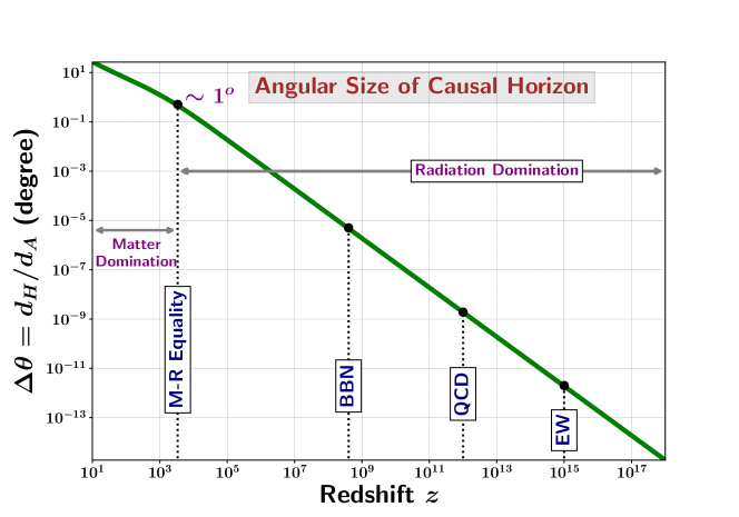
Figure 3: Angular size of the causal horizon, given by Eq. (34), is plotted as a function of redshift for the standard ${\rm\Lambda}$CDM universe.

Another intuitive way to understand the Horizon problem is to look at the conformal time elapsed between the beginning of the universe, until a given epoch, defined as,

$$\Delta\tau=\int_{0}^{t}\,\frac{{\rm d}\tilde{t}}{a(\tilde{t})}=\int_{0}^{a}\,\frac{{\rm d}\tilde{a}}{\tilde{a}^{2}\,H(\tilde{a})}\,\,$$ (38)

which is analogous to the comoving causal horizon $r_{H}=\frac{d_{H}}{a}$, and hence gives us the separation between comoving coordinates that have been in causal contact since the beginning of the universe. The advantage of using conformal time in eliciting the horizon problem is the following. The FLRW metric given in Eq. (2) can be written in terms of conformal time as

$${\rm d}s^{2}=a^{2}(\tau)\left[-{\rm d}\tau^{2}+\,\delta_{ij}\,{\rm d}x^{i}{\rm d}x^{j}\right]\,,$$ (39)

which is conformally equivalent to the metric of the Minkowski space-time. Hence, the causal structure of FLRW space-time in terms of the conformal time is equivalent to that of the Minkowski space-time. So we can draw the usual space-time diagrams of Special Relativity with light cones subtending $45^{\circ}$ angle with the space and time axes. Hence, for diametrically opposite points in the CMB (which are at a fixed comoving distance from us) to be in causal contact with each other, the conformal time elapsed between the beginning of the universe and recombination should be greater than the conformal time elapsed between recombination and today. However, from Eq. (38), we have

$$\Delta\tau(a)\propto\begin{cases}a\,;&{\rm RD}\,,\\ a^{1/2}\,;&{\rm MD}\,,\end{cases}$$ (40)

which indicates that the conformal time grows with scale factor in the standard Big Bang theory and hence its size would be extremely small at the time of recombination, namely,

$$\Delta\tau\left(a_{\rm BB}\to a_{\rm CMB}\right)\,\ll\,\Delta\tau\left(a_{\rm CMB}\to a_{0}\right)\,.$$

Hence, diametrically opposite points in the CMB sky could not have been in causal contact since the birth of the universe, leading to the Horizon problem. This is illustrated in Fig. 4.

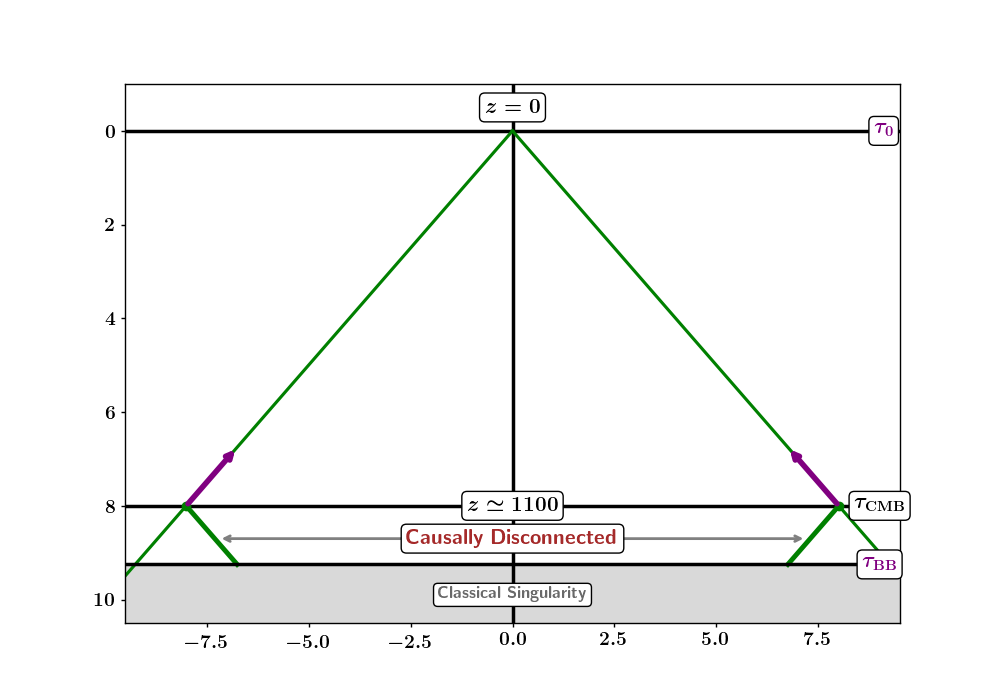
Figure 4: The conformal causal diagram of the universe in the standard cosmology where the universe began in the hot Big Bang phase being radiation dominated. This figure schematically illustrates the fact that diametrically opposite points in the CMB sky could not have been in causal contact by the time of photon decoupling due to the lack of enough conformal time between the classical Big Bang singularity and the epoch of recombination.

So we conclude that, in the standard hot Big Bang theory, the early universe seems to be comprised of an unnaturally large number of causally disconnected regions, each possessing the same average temperature and density. This again demands for a physical mechanism prior to the standard hot Big Bang phase which can bring the entire sky into causal contact by the commencement of the hot Big Bang phase.

3.3 Super-Hubble correlation of primordial perturbations

Towards the end of Sec. 2, we mentioned that the primordial seed fluctuations of the comoving curvature perturbation $\zeta$ are nearly adiabatic, Gaussian and almost scale-invariant. However, more interestingly, these fluctuations have a non-vanishing two-point auto-correlation (power spectrum or variance) at angular scales that are larger than the angular size of the Hubble radius in the CMB sky. This can be easily seen from the low-$l$ (large scale) angular power spectrum of temperature fluctuations in the CMB sky (see Fig. 1 of Ref. [2]). The physical size of the Hubble radius is defined as

$$R_{H}=\frac{1}{H}=\frac{1}{H_{i}}\,\left(\frac{a}{a_{i}}\right)^{\frac{3(1+w)}{2}}\,,$$ (41)

while the size of the comoving Hubble radius is given by

$$r_{h}=(aH)^{-1}=(a_{i}H_{i})^{-1}\,\left(\frac{a}{a_{i}}\right)^{\frac{1+3w}{2}}\,.$$ (42)

Comparing Eq. (31) with Eq. (41), we find the relation between the causal horizon and Hubble radius in a decelerating single component dominated universe to be

$$d_{H}=\left(\frac{2}{1+3w}\right)\,R_{H}.$$ (43)

Thus, a super-Hubble correlation in a decelerating universe also implies a super-Horizon correlation of primordial fluctuations. This naturally demands for a physical explanation. At this point, it is important to remind the reader of the crucial distinction between causal horizon and Hubble radius. Size of the causal horizon is determined by integrating over the expansion history, as can be seen from Eq. (28). Consequently, if the distance between two points in space at a given epoch is larger than the physical size of the causal horizon, then these two points were never in causal contact since the beginning of the universe. While, if two points are separated by a distance greater than the physical size of the Hubble radius at some epoch, then these points are not in causal contact at that epoch. However, this does not necessarily imply they were never in causal contact in the past.

Hence the resolution of the conundrum of super-Hubble primordial correlations involves the existence of an epoch prior to the hot Big Bang phase where the Hubble radius evolves differently as compared to the causal horizon. In fact, as we will see, in an accelerating universe the natural spacetime dynamics leads to length scales constantly being stretched outside the Hubble radius without violating causality.

4 The inflationary hypothesis

In this section, we will stress that a sufficiently long epoch of accelerated expansion of space prior to the hot Big Bang phase naturally addresses all of the above problems and provides appropriate initial conditions for the hot Big Bang phase. Hence, the hot Big Bang phase in the standard Big Bang theory is not the beginning of our universe, but rather the end of an earlier epoch of accelerated expansion. In fact, this is the key message that these lecture notes are meant to convey.

The resolution of the problems of fine tuning of initial conditions emerges from the key observation that all three initial condition problems of the hot Big Bang stem from one common dynamics of the decelerating universe, that is the fact that the comoving Hubble radius $r_{h}=(aH)^{-1}$ increases with time, as can be seen from Eqs. (21), (29) and (42). Consequently, we can address all of them by assuming a sufficiently long epoch of expansion history where the comoving Hubble radius decreases with time, namely

$$\frac{{\rm d}}{{\rm d}t}\left(aH\right)^{-1}<0\leavevmode\nobreak\ \Rightarrow\leavevmode\nobreak\ 1+\frac{\dot{H}}{H^{2}}>0\leavevmode\nobreak\ \Rightarrow\leavevmode\nobreak\ \ddot{a}>0,$$ (44)

which is equivalent to an accelerating or inflating universe. Let us explicitly demonstrate how inflation addresses the flatness and horizon problems, and generates fluctuations that are correlated over super-Hubble scales.

4.1 Addressing the flatness problem

The initial flatness problem of the hot Big Bang phase discussed in Sec. 3.1 can be naturally solved provided if there was a long enough period of inflation prior to the radiation domination, as discussed above. In particular, for a perfect fluid with EoS $w$ to drive inflation, we need

$$\frac{\ddot{a}}{a}>0\quad\Rightarrow\quad 1\,+\,3\,w<0\quad\Rightarrow\quad w<-1/3\,,$$

leading to

$$|\Omega_{\rm tot}(a)-1|=|\Omega_{\rm tot}(a_{i})-1|\,\left(\frac{a}{a_{i}}\right)^{-|1+3w|}\leavevmode\nobreak\ \propto\leavevmode\nobreak\ a^{-|1+3w|}\,.$$ (45)

Hence, during inflation, $|\Omega_{\rm tot}-1|$ or equivalently $|\Omega_{K}|$ decreases with time which results in $\Omega_{\rm tot}(a)$ being driven towards unity, as long as inflation lasts long enough. In particular, for near exponential inflation sourced by an effective cosmological constant $w\simeq-1$, we have

$$|\Omega_{\rm tot}(a_{\rm end})-1|=|\Omega_{\rm tot}(a_{i})-1|\,e^{-2\,\Delta N}\,,$$ (46)

where $\Delta N=\ln\left(a_{\rm end}/a_{i}\right)$ is the total number of e-folds of accelerated expansion during inflation. Assuming inflation began at some higher energy scale closer to the GUT scale, with the curvature density being of the same order as the total density i.e. of order unity,

$$|\Omega_{K}(a_{i})|=|\Omega_{\rm tot}(a_{i})-1|\approx\mathcal{O}(1)\,,$$

Eq. (46) leads to

$$|\Omega_{\rm tot}(a_{\rm end})-1|\approx\mathcal{O}(1)\times e^{-2\,\Delta N}\,.$$

We see that $|\Omega_{\rm tot}(a_{\rm end})-1|\leq 10^{-56}$ for $\Delta N\geq 64.47$. This demonstrates that starting from an order unity curvature term at the GUT scale, about $65$ e-folds of inflation is enough to result in $\Omega_{0K}\leq 10^{-2}$. In other words, if the hot Big Bang is not the beginning of our universe, but rather is the end of a sufficiently long enough period of inflation, then we expect the spatial curvature to be negligible at the present epoch.

4.2 Addressing the horizon problem

During the rapidly accelerated expansion of space, for which $\frac{1+3w}{2}<0$, the conformal time $\tau$ can be obtained by integrating Eq. (38) to be

$$\tau=\tau_{1}+\frac{1}{a_{1}H_{1}}\,\left|\frac{2}{1+3w}\right|\,\left[1-\left(\frac{a_{1}}{a}\right)^{|1+3w|/2}\right]\,,$$ (47)

where $a_{1}$ is the scale factor at some reference epoch $\tau_{1}$. Eq. (47) shows that the conformal time is negative and diverges at early times, $\tau\to-\infty$ as $a\to 0$. Thus, accelerated expansion yields a substantial amount of conformal time during the early history of the universe prior to $\tau=\tau_{1}$, which in turn brings together a large region of comoving space into causal contact going back in the past.

In order to see this more explicitly, let us specialise to the case of exponential inflation, for which

$$\tau=\tau_{1}+\frac{1}{a_{1}H}-\frac{1}{aH}\,.$$

Taking $\tau_{1}=-1/(a_{1}H)$, we derive the expression for the conformal time in de Sitter spacetime to be

$$\boxed{\tau=-\frac{1}{aH}}\,,$$ (48)

which tells us that the conformal time is large and negative at early times during inflation, while it approaches zero towards the end of inflation, namely,

$$\tau\,:\,-\infty\,\longrightarrow\,0$$

during inflation. Hence a sufficient amount of exponential expansion in the early universe results in bringing the entire CMB sky in causal contact, as shown schematically in Fig. 5.

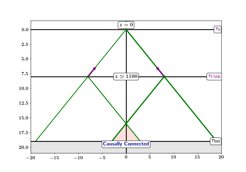
Figure 5: The conformal causal diagram of the universe in the presence of an early stage of exponential inflation before the commencement of the hot Big Bang phase. From this figure, it is clear that diametrically opposite points in the CMB sky could have easily been in causal contact if there was a sufficiently long period of inflation prior to the hot Big Bang phase, which facilitates for a substantial amount of conformal time to have elapsed in the past light cone.

Alternatively, the physical size of the causal horizon $d_{H}$ in an accelerated universe becomes much larger than the Hubble radius. In fact at the end of inflation, we have

$$d_{H}\sim e^{\Delta N}\,R_{H}\,,$$

where $\Delta N$ is the total number of e-folds of expansion of space during inflation. Hence the horizon size at any epoch in the post inflationary universe is much larger than the Hubble radius, which naturally resolves the horizon problem discussed in Sec. 3.2.

4.3 Generating super-Hubble fluctuations

During the accelerated expansion of space, the comoving Hubble radius, $r_{h}$, starts shrinking with time, i.e.

$$r_{h}\propto a^{-\frac{|1+3w|}{2}}\,$$

as can be seen from from Eq. (42). Since comoving length scales corresponding to the fluctuations remain fixed with time, a shrinking comoving Hubble radius causes length scales, that were initially shorter than the Hubble radius (known as sub-Hubble modes), to become larger than the Hubble radius (super-Hubble) at late times. Thus the rapid accelerated expansion of space during inflation dynamically stretches the wavelength of (initial) sub-Hubble fluctuations to large super-Hubble scales at late times. A long enough period of inflation ensures that by the end of inflation, all of the observable length scales in the CMB sky, which started out being sub-Hubble, would have become super-Hubble. On super-Hubble scales the comoving curvature fluctuations $\zeta$ remain frozen/constant, as we will see in Sec. 6.2.

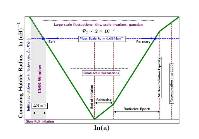
Figure 6: This figure schematically illustrates the evolution of the comoving Hubble radius $(aH)^{-1}$ with scale factor, both plotted on a logarithmic scale (we have assumed $H$ to be almost constant during inflation). $(aH)^{-1}$ decreases which causes physical scales to exit the Hubble radius during inflation. As $(aH)^{-1}$ rises during the post-inflationary epochs, physical scales begin to re-enter the Hubble radius. The CMB pivot scale, as used by the Planck mission, is set at $k_{*}=0.05\,{\rm Mpc}^{-1}$ and has been depicted by the dashed blue line.

Inflation thus provides a causal mechanism to generate correlated primordial fluctuations on super-Hubble scales. The final state of inflationary fluctuations then acts as the initial seed fluctuations for the hot Big Bang phase. The transition epoch between the end of inflation and the beginning of the hot Big Bang phase is called reheating (as mentioned before) which can last up to a few e-folds of (decelerated) expansion. Evolution of the Hubble radius during and after inflation is illustrated schematically in Fig. 6 using a comoving scale, and in Fig. 7 using the physical scale, assuming exponential expansion of space during inflation. The blue coloured lines indicate fluctuations of different wavelengths, while the blue stars indicate the Hubble-exit of the CMB pivot scale during inflation and, later, its Hubble-entry after the end of inflation. Figs. 6 and 7 demonstrate that long wavelength fluctuations, which made their Hubble-exit at early times during inflation, re-entered the Hubble radius at late times closer to the present epoch. On the other hand, shorter wavelength fluctuations became super-Hubble towards the end of inflation, and subsequently made their Hubble re-entry quite early after inflation had ended.

As the comoving Hubble radius began to increase (because of the decelerated expansion of space after inflation) and one by one, these frozen fluctuations became sub-Hubble again, they began evolving with time. Eventually, the fluctuations were amplified by gravitational instability to form the LSS of the universe. Note that several sources in the literature extensively refer to Hubble-exit and Hubble-entry as ‘horizon exit’ and ‘horizon entry’. However, in these lecture notes, we have made an attempt to avoid such phrases and stick to the more accurate phrases: Hubble-exit and Hubble-entry.

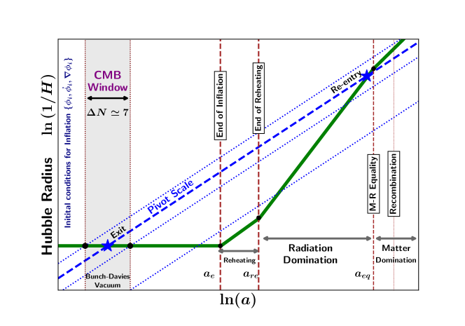
Figure 7: Evolution of the physical Hubble radius $1/H$ is shown with scale factor (both plotted in logarithmic scale). The physical Hubble radius $1/H$ stays almost constant during inflation which causes physical scales to exit the Hubble radius during inflation. $1/H$ rises in the post-inflationary epoch and the physical scales begin to re-enter the Hubble radius.

Hubble-exit and entry can be understood intuitively as follows: during inflation, accelerated expansion rapidly stretched the wavelengths of fluctuations. Eventually the frequencies of oscillations of these modes fell below the rate of expansion of space. Or equivalently, we say the modes became super-Hubble. Similarly after the end of inflation, the rate of expansion of space fell rapidly. Hence fluctuations which were super-Hubble can eventually began to oscillate once the rate of expansion fell below their frequencies of oscillations. Or equivalently, we say the fluctuation modes became sub-Hubble after their Hubble re-entry.

In general, a variety of functional forms of the scale factor $a(t)$ which supports accelerated expansion of space, i.e. $\ddot{a}>0$, can address the initial conditions problem of the hot Big Bang theory, as long as inflation lasts long enough. However, from the latest CMB observations we know that if inflation happened, then the accelerated expansion of space must have been nearly exponential, $a(t)\propto e^{Ht}$, where $H$ is almost constant during inflation. Hence we will primarily focus on the quasi-de Sitter expansion of space during inflation. Typically a period of quasi-de Sitter inflation lasting for at least 60–70 e-folds of expansion is enough to address the initial conditions for the hot Big Bang phase, as discussed in App. B. The comoving Hubble radius plotted in Fig. 6 is particularly convenient to refer to because of the symmetry between its fall during inflation and rise in the radiation dominated epoch. In fact, Fig. 6 demonstrates that in order to ensure that the largest observable length scales are sub-Hubble during inflation, the universe must spend approximately same number of e-folds of inflationary evolution as it does in the post-inflationary epoch.

In Einstein’s gravity, an accelerated expansion of space can be sourced by a negative pressure substance satisfying $w<-1/3$, as can be seen from Eq. (16). A natural candidate to drive inflation is a singlet scalar field $\varphi$ with self-interaction potential $V(\varphi)$ possessing a low enough effective mass $m_{\rm eff}^{2}\equiv\frac{{\rm d}^{2}V(\varphi)}{{\rm d}\varphi^{2}}\lesssim H^{2}$. Since by now the curious reader might have become bored with preceding long and detailed discussions on inflationary kinematics, let us move forward to delve into the rich physics of single field inflationary dynamics without further delay.

5 Scalar field dynamics of inflation

In these lecture notes, we focus on the simplest inflationary scenario sourced by a single scalar field $\varphi$, known as the inflaton field, with a self-interaction potential $V(\varphi)$ which is minimally coupled to gravity. The full system of Gravity + Scalar field is described by the action

$$S[\varphi]=\int{\rm d}^{4}x\,\sqrt{-g}\;{\cal L}(X,\varphi)\,,$$ (49)

where the Lagrangian density ${\cal L}(X,\varphi)$ is a function of the field $\varphi$ and the kinetic term

$$X\equiv\frac{1}{2}\,\partial_{\mu}\varphi\;\partial^{\mu}\varphi=\frac{1}{2}\,\partial_{\mu}\varphi\;\partial_{\nu}\varphi\,g^{\mu\nu}\,.$$ (50)

Varying Eq. (49) with respect to $\varphi$ results in the Euler-Lagrange field equation for the evolution of the scalar field, given by

$$\frac{\partial{\cal L}}{\partial\varphi}-\left(\frac{1}{\sqrt{-g}}\right)\partial_{\mu}\left(\sqrt{-g}\frac{\partial{\cal L}}{\partial\left(\partial_{\mu}\varphi\right)}\right)=0\,.$$ (51)

The energy-momentum tensor of the scalar field associated with the space-time translational invariance of the action in Eq. (49) is given by

$$T^{\mu\nu}=\left(\frac{\partial{\cal L}}{\partial X}\right)\,\left(\partial^{\mu}\varphi\;\partial^{\nu}\varphi\right)-g^{\mu\nu}\,{\cal L}\leavevmode\nobreak\ .$$ (52)

In Sec. 5.2, we will study linear perturbation theory during inflation. For that purpose, we will split the system into time-dependent uniform background and space (and time) dependent perturbations. We start with the discussion of the background scalar field $\phi(t)$ and space-time dynamics, described by the FLRW metric defined below.

5.1 Background dynamics during inflation

Specializing to a spatially flat FLRW universe and a homogeneous part $\phi(t)$ of the scalar field $\varphi(t,\vec{x})$, one finds

$${\rm d}s^{2}=-{\rm d}t^{2}+a^{2}(t)\;\left[{\rm d}x^{2}+{\rm d}y^{2}+{\rm d}z^{2}\right]\,,$$ (53)

$$T^{\mu}_{\;\>\;\nu}\equiv\mathrm{diag}\left(-\rho_{{}_{\phi}},\,p_{{}_{\phi}}\,\,p_{{}_{\phi}},\,p_{{}_{\phi}}\right)\,,$$ (54)

where the energy density $\rho_{{}_{\phi}}$, and pressure $p_{{}_{\phi}}$, of the homogeneous inflaton field are given by

$$\rho_{{}_{\phi}} = \left(\frac{\partial{\cal L}}{\partial X}\right)\,(2\,X)-{\cal L}\,,$$ (55)

$$p_{{}_{\phi}} = {\cal L},$$ (56)

with $X=-\frac{1}{2}\dot{\phi}^{2}$. Evolution of the scale factor $a(t)$ is governed by the Friedmann equations

$$\left(\frac{\dot{a}}{a}\right)^{2}\equiv H^{2}=\frac{1}{3m_{p}^{2}}\,\rho_{{}_{\phi}},$$ (57)

$$\frac{\ddot{a}}{a}\equiv\dot{H}+H^{2}=-\frac{1}{6m_{p}^{2}}\,\left(\rho_{{}_{\phi}}+3\,p_{{}_{\phi}}\right),$$ (58)

where $H\equiv\dot{a}/a$ is the Hubble parameter and $\rho_{{}_{\phi}}$ satisfies the conservation equation

$${\dot{\rho}_{{}_{\phi}}}=-3\,H\left(\rho_{{}_{\phi}}+p_{{}_{\phi}}\right)\leavevmode\nobreak\ .$$ (59)

In the standard inflationary paradigm, inflation is sourced by a scalar field $\phi$ with a potential $V(\phi)$ (see Fig. 8) which is minimally coupled to gravity. For a canonical scalar field, the Lagrangian density takes the form

$${\cal L}(X,\phi)=-X-V(\phi)\,.$$ (60)

Substituting Eq. (60) into Eq. (55) and Eq. (56), the expressions for energy density and pressure become

$$\rho_{{}_{\phi}} = \frac{1}{2}{\dot{\phi}}^{2}+\;V(\phi)\,,$$

$$p_{{}_{\phi}} = \frac{1}{2}{\dot{\phi}}^{2}-\;V(\phi)\,,\leavevmode\nobreak\ \leavevmode\nobreak\$$ (61)

consequently the two Friedmann Eqs. (57), (58) and the equation of motion Eq. (59) become

$$H^{2}=\frac{1}{3m_{p}^{2}}\,\rho_{\phi}=\frac{1}{3m_{p}^{2}}\left[\frac{1}{2}{\dot{\phi}}^{2}+V(\phi)\right],$$ (62)

$$\dot{H}\equiv\frac{\ddot{a}}{a}-H^{2}=-\frac{1}{2m_{p}^{2}}\,\dot{\phi}^{2}\,,$$ (63)

$${\ddot{\phi}}+3\,H{\dot{\phi}}+V_{,\phi}=0\,.$$ (64)

The evolution of various physical quantities during inflation is usually described with respect to the number of e-folds of expansion which is given by $N=\ln(a/a_{i})$, where $a_{i}$ is some arbitrary epoch at very early times during inflation. It is informative to write and solve the Friedmann equations in terms of the number of e-folds as follows:

$$H^{2} = \frac{V(\phi)}{3\,m_{p}^{2}-\frac{1}{2}\left(\frac{{\rm d}\phi}{{\rm d}N}\right)^{2}}\,;$$ (65)

$$\frac{{\rm d}H}{{\rm d}N} = -H\,\frac{1}{2m_{p}^{2}}\left(\frac{{\rm d}\phi}{{\rm d}N}\right)^{2}\,;$$ (66)

$$\frac{{\rm d}^{2}\phi}{{\rm d}N^{2}} = -\frac{{\rm d}\phi}{{\rm d}N}\left(3+\frac{1}{H}\,\frac{{\rm d}H}{{\rm d}N}\right)-\frac{1}{H^{2}}\,V_{,\phi}\,.$$ (67)

A better physical quantity to depict any epoch with scale factor $a$ during the inflationary expansion is the number of e-folds before the end of inflation which is defined as

$$N_{e}(a)=\ln\left(\frac{a_{e}}{a}\right)=\int_{t}^{t_{e}}H(t)\,{\rm d}t,$$ (68)

where $H(t)$ is the Hubble parameter during inflation, and $a_{e}$ denotes the scale factor at the end of inflation, hence $N_{e}=0$ corresponds to the end of inflation. Typically a period of quasi-de Sitter (exponential) inflation lasting for at least 60–70 e-folds is required in order to address the problems of the standard hot Big Bang model discussed in Sec. 3. We denote $N_{*}$ as the number of e-folds (before the end of inflation) when the CMB pivot scale

$$k_{*}=(aH)_{*}=0.05\leavevmode\nobreak\ \rm Mpc^{-1}$$ (69)

left the comoving Hubble radius during inflation. Typically $N_{*}\in[50,\,60]$ depending upon the details of reheating after inflation (see Ref. [73] and App. B).

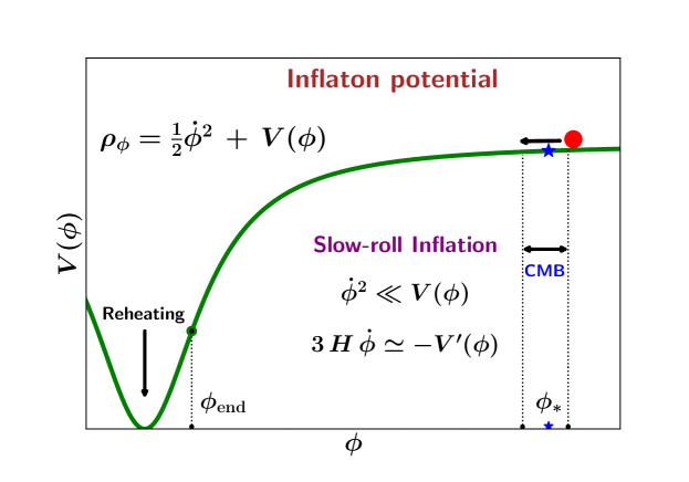
Figure 8: This figure schematically depicts a prototypical inflaton potential (solid green curve). The ‘CMB window’ represents field values corresponding to the Hubble-exit epochs of scales $k\in\left[0.0005,0.5\right]\leavevmode\nobreak\ {\rm Mpc}^{-1}$ that are observationally accessible with the latest CMB missions.

The quasi-de Sitter like phase corresponds to the inflaton field rolling slowly down the potential $V(\phi)$. For a variety of functional forms of the inflaton potential $V(\phi)$, there exists a slow-roll regime of inflation, ensured by the presence of the Hubble friction term [74, 33, 9, 75, 76, 77] in Eq. (64). This slow-roll regime can be conveniently characterised by the first two kinematic Hubble slow-roll parameters $\epsilon_{H}$, $\eta_{H}$, defined by  [78, 9]

$$\epsilon_{H} = -\frac{\dot{H}}{H^{2}}=-\frac{{\rm d}\,\ln{H}}{{\rm d}N}=\frac{1}{2m_{p}^{2}}\,\frac{\dot{\phi}^{2}}{H^{2}}\,;$$ (70)

$$\eta_{H} = -\frac{\ddot{\phi}}{H\dot{\phi}}=\epsilon_{H}-\frac{1}{2\epsilon_{H}}\,\frac{{\rm d}\epsilon_{H}}{{\rm d}N}\,,$$ (71)

where the slow-roll regime of inflation corresponds to

$$\epsilon_{H},\leavevmode\nobreak\ |\eta_{H}|\ll 1\,.$$ (72)

Note that $\epsilon_{H}\geq 0$, while $\eta_{H}$ may be negative or positive depending on whether $\epsilon_{H}$ is increasing or decreasing with time. Using the definition of the Hubble parameter, $H=\dot{a}/a$, we have $\ddot{a}/a=\dot{H}+H^{2}=H^{2}(1+\dot{H}/H^{2})$. From the expression for $\epsilon_{H}$ in Eq. (70), it is easy to see that

$$\frac{\ddot{a}}{a}=H^{2}\,\big{(}1-\epsilon_{H}\big{)}\,,$$ (73)

which implies that the universe accelerates, ${\ddot{a}}>0$, when $\epsilon_{H}<1$. Using equation (62), the expression for $\epsilon_{H}$ in Eq. (70) reduces to $\epsilon_{H}\simeq\frac{3}{2}\frac{\dot{\phi}^{2}}{V}$ when ${\dot{\phi}}^{2}\ll V$. In fact, under the slow-roll conditions in Eq. (72), the Friedmann equations given by Eqs. (62) and (64) take the form

$$H^{2} \simeq \frac{V(\phi)}{3\,m_{p}^{2}}\,;$$ (74)

$$\dot{\phi} \simeq -\frac{V_{,\phi}}{3\,H}\,.$$ (75)

The last expression is a consequence of $|\eta_{H}|\ll 1$, which ensures that the inflaton speed does not change too rapidly, resulting in a long enough period of accelerated expansion before the end of inflation. The classical slow-roll dynamics corresponding to Eq. (75) during inflation is similar to the slow terminal motion of an object where the attractive force and the restraining drag/friction force are almost balanced with each other. The slow-roll conditions in Eqs. (74) and (75) can be combined to obtain the slow-roll trajectory described by

$$\boxed{\dot{\phi}\simeq-\frac{m_{p}}{\sqrt{3}}\,\frac{V_{,\phi}}{\sqrt{V(\phi)}}}\,.$$ (76)

It is well known that the slow-roll trajectory is actually a local attractor for a number of different models of inflation, see Refs. [74, 33, 9, 75, 76, 77]. The slow-roll regime of inflation is described more systematically in terms of the Hubble flow parameters $\epsilon_{n}$ defined by

$$\epsilon_{n+1}=\frac{{\rm d}\ln\,\epsilon_{n}}{{\rm d}N}\,;\quad{\rm with}\quad\epsilon_{1}=\epsilon_{H}\,.$$ (77)

Accordingly, from Eq. (71), the second Hubble flow parameter $\epsilon_{2}$ is related to $\epsilon_{H}$ and $\eta_{H}$ via

$$\epsilon_{2}=2\left(\epsilon_{H}-\eta_{H}\right)\,.$$ (78)

Apart from the aforementioned kinematic slow-roll parameters, the slow-roll regime is also often characterised by the dynamical potential slow-roll parameters [9], defined by

$$\epsilon_{{}_{V}} = \frac{m_{p}^{2}}{2}\left(\frac{V_{,\phi}}{V}\right)^{2}\,;$$ (79)

$$\eta_{{}_{V}} = m_{p}^{2}\,\left(\frac{V_{,\phi\phi}}{V}\right)\,.$$ (80)

For small values of these parameters $\epsilon_{H}\ll 1,\,\eta_{H}\ll 1$, from Eqs. (70) and (75) one finds $\epsilon_{H}\simeq V_{,\phi}^{2}/(18\,m_{p}^{2}\,H^{4})$, which, using Eq. (74) becomes

$$\epsilon_{H}\simeq\frac{m_{p}^{2}}{2}\left(\frac{V_{,\phi}}{V}\right)^{2}=\epsilon_{{}_{V}}\,.$$

Similarly, taking a time derivative of Eq. (75) and incorporating it into Eq. (74), we get

$$\eta_{H}=-\frac{\ddot{\phi}}{H\dot{\phi}}\simeq\eta_{V}-\epsilon_{V}\,.$$

The end of inflation is marked by

$$\epsilon_{H}(\phi_{e})=1\simeq\epsilon_{{}_{V}}(\phi_{e})\,.$$

Furthermore, under the slow-roll approximations, since $\epsilon_{H}\simeq\epsilon_{{}_{V}}$, the Hubble-exit of the CMB pivot scale $k_{*}$ is denoted by the number of e-folds before the end of inflation $N_{*}$, which can be obtained from Eq. (68) to be

$$\boxed{N_{*}=\int_{t_{*}}^{t_{e}}{\rm d}t\,H(t)\leavevmode\nobreak\ =\leavevmode\nobreak\ \frac{1}{m_{p}}\,\int_{\phi_{e}}^{\phi_{*}}\,\frac{d\phi}{\sqrt{2\,\epsilon_{H}}}\leavevmode\nobreak\ \simeq\leavevmode\nobreak\ \frac{1}{m_{p}}\,\int_{\phi_{e}}^{\phi_{*}}\,\frac{d\phi}{\sqrt{2\,\epsilon_{{}_{V}}(\phi)}}}\,.$$ (81)

The above formula is quite useful in computing the value of $\phi_{*}$ for a given potential that supports slow roll, as we will see in Sec. 7.2.

Before proceeding further, we remind the reader of the distinction between the quasi-de Sitter (qdS) and slow-roll (SR) approximations.

• Quasi-de Sitter inflation corresponds to the condition $\epsilon_{H}\ll 1\leavevmode\nobreak\ \Rightarrow\leavevmode\nobreak\ \frac{1}{2}\,\dot{\phi}^{2}\ll V(\phi)\,.$

• Slow-roll inflation corresponds to both $\epsilon_{H},\,|\eta_{H}|\ll 1\,.$

Note that one can deviate from the slow-roll regime by having $|\eta_{H}|\geq 1$ while still maintaining the qdS expansion by keeping $\epsilon_{H}\ll 1$, which is exactly what happens during the so-called ultra slow-roll (USR) inflation [79, 80, 81, 82, 83]. This distinction will not be important for the rest of these lecture notes in the present version. Under either of the aforementioned assumptions, the conformal time, $\tau$, is given by Eq. (48) to be $\tau\simeq-1/(aH)$.

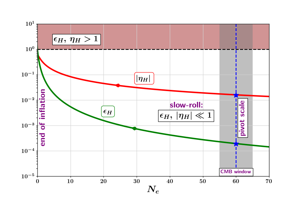
Figure 9: The evolution of the slow-roll parameters $\epsilon_{H}$ and $\eta_{H}$ is shown as a function of the number of e-folds before the end of inflation $N_{e}$ for Starobinsky potential (218). From this plot, it is easy to notice that at early times when $N_{e}\gg 1$, the slow-roll conditions are satisfied i.e $\epsilon_{H},\,|\eta_{H}|\ll 1$. However, the slow-roll conditions are violated towards the end of inflation (marked by $N_{e}=0$ and $\epsilon_{H}=1$).

During inflation, since the inflaton evolves monotonically, one can describe the evolution of the background dynamics by re-writing Eqs. (62)–(64) such that $\phi$ behaves as a time variable. Inflationary dynamics in terms of a $\phi$-clock is known as the Hamilton-Jacobi formalism [78] of inflation, discussed in App. C.

We conclude that a scalar field with a sufficiently shallow potential $V(\phi)$ with $\epsilon_{{}_{V}}\ll 1$ leads to nearly exponential (qdS) expansion of the background space-time during inflation, which successfully addresses the fine tuning of initial conditions for the background evolution, such as the flatness and the horizon problems, discussed in Secs. 3.1 and 3.2. As inflation progresses, since the friction coefficient $H$ falls with time (although slowly) the slow-roll parameter $\epsilon_{H}$ (also $\epsilon_{{}_{V}}$) increases and eventually becomes greater than unity, thus terminating the accelerated expansion of space. Towards the end of inflation, slow-roll conditions are violated (see Fig. 9). After the end of inflation, the inflaton field oscillates around the minimum of the potential. Subsequently, the oscillating inflaton condensate decays into matter and radiation, via a process called reheating, leading to the commencement of the hot Big Bang phase. We will return to the topic of reheating in Sec. 8.

Next, we move on to discuss how quantum fluctuations during inflation provides a natural mechanism for generating the initial seeds of structure formation in the universe.

5.2 Quantum fluctuations during Inflation

Our system is a canonical scalar field minimally coupled to gravity whose action is given by

$$S[g_{\mu\nu},\varphi]=\int\,{\rm d}^{4}x\,\sqrt{-g}\,\left(\,\frac{m_{p}^{2}}{2}\,R-\frac{1}{2}\,\partial_{\mu}\varphi\,\partial_{\nu}\varphi\,g^{\mu\nu}-V(\varphi)\right).$$ (82)

In perturbation theory, we split the metric and inflaton field into their corresponding homogeneous background pieces and fluctuations, namely

$$g_{\mu\nu}(t,\vec{x})=\bar{g}_{\mu\nu}(t)+\delta g_{\mu\nu}(t,\vec{x})\,;\quad\varphi(t,\vec{x})=\phi(t)+\delta\varphi(t,\vec{x})\,.$$

Note that the perturbed metric $\delta g_{\mu\nu}$ has 10 degrees of freedom, out of which only two are independent, while the rest are fixed by gauge freedom, and the Hamiltonian and momentum constraints. The perturbed line element in the Arnowitt-Deser-Misner (ADM) formalism [84, 85] can be written as

$${\rm d}s^{2}=-\alpha^{2}\,{\rm d}t^{2}+\gamma_{ij}\left({\rm d}x^{i}+\beta^{i}\,{\rm d}t\right)\left({\rm d}x^{j}+\beta^{j}\,{\rm d}t\right)\,,$$ (83)

where $\alpha=1+\delta\alpha$ and $\beta^{i}$ are the lapse and shift functions, while $\gamma_{ij}$ are the dynamical metric perturbations.

In these lecture notes, we will skip the detailed discussion of relativistic cosmological perturbation theory (which is an extremely important topic) and direct the interested readers to Refs. [86, 87, 9, 88, 89, 90, 35]. For the purpose of pedagogy and simplicity, we work in the comoving gauge defined by

$$\delta\varphi(t,\vec{x})=0\,;\quad\gamma_{ij}(t,\vec{x})=a^{2}\bigl{[}\bigl{(}1+2\,\zeta(t,\vec{x})\bigr{)}\,\delta_{ij}\,+\,h_{ij}(t,\vec{x})\bigr{]}\,.$$ (84)

In particular, two gauge-invariant light fields are guaranteed to exist in the single field inflationary scenario, which are

1. Scalar-type comoving curvature perturbations   $\zeta(t,\vec{x})\,;$

2. Tensor-type transverse and traceless perturbations   $h_{ij}(t,\vec{x})\,.$

The scalar fluctuations would eventually induce density and temperature perturbations in the hot Big Bang phase, and subsequently the large scale structure of the universe, while the tensor fluctuations propagate as gravitational waves (GWs) at late times and constitute a stochastic cosmological background of GWs.

The perturbed action in the comoving gauge can be expressed as

$$S[g_{\mu\nu},\varphi]=S_{B}[\bar{g}_{\mu\nu},\phi]+S^{(2)}[\zeta]+S^{(2)}[h_{ij}]+S_{\rm int}[\zeta,h_{ij}]\,,$$ (85)

where $S_{B}[\bar{g}_{\mu\nu},\phi]$ is the background action, while $S^{(2)}[\zeta],\,S^{(2)}[h_{ij}]$ are the quadratic actions for the scalar and tensor fluctuations (which results in linear field equations for the fluctuations). The term $S_{\rm int}[\zeta,h_{ij}]$ is the action for fluctuations beyond the linear order which we do not discuss in these lecture notes and direct the interested readers to Refs. [9, 85, 91].

The background action $S_{B}[\bar{g}_{\mu\nu},\phi]$ leads to the familiar Friedmann Equations

$$H^{2}=\left(\frac{\dot{a}}{a}\right)^{2}=\left(\frac{1}{3m_{p}^{2}}\right)\rho_{{}_{\phi}},$$

$$\dot{H}=-\frac{1}{2m_{p}^{2}}\dot{\phi}^{2}\leavevmode\nobreak\ ,$$

which result in an accelerated expansion of space for a suitable potential $V(\phi)$ at the background level. Under slow-roll condition $\epsilon_{H}\ll 1$, we get quasi-dS expansion $a(t)\sim e^{Ht}$.

The quadratic action for the (linear) scalar-type fluctuations in the comoving gauge is

$$S^{(2)}[\zeta]=\frac{1}{2}\int{\rm d}\tau\,{\rm d}^{3}\vec{x}\leavevmode\nobreak\ \left(am_{p}\sqrt{2\epsilon_{H}}\right)^{2}\,\left[(\zeta^{\prime})^{2}-(\partial_{i}\zeta)^{2}\right]\,,$$

and for the (linear) tensor-type perturbations is

$$S^{(2)}[h_{ij}]=\frac{1}{2}\int{\rm d}\tau\,{\rm d}^{3}\vec{x}\leavevmode\nobreak\ \,\left(\frac{a\,m_{p}}{2}\right)^{2}\left[(h^{\prime}_{ij})^{2}-(\partial_{l}h_{ij})^{2}\leavevmode\nobreak\ .\right]$$

At linear order in perturbation theory, the scalars, vectors and tensors are decoupled (the so-called SVT decomposition theorem), and hence their evolution during inflation can be studied separately, as discussed in Ref. [9]. We will begin with scalar fluctuations and then move on to study tensor fluctuations. In the following, we describe the evolution of perturbations during inflation generated by quantum fluctuations at linear order in perturbation theory. Note that the fluctuations are categorized into scalars, vectors and tensors depending on their transformation properties under the rotation group ${\rm SO}(3)$ on the three dimensional spatial hypersurfaces.

In the following section, we will delve into the study of scalar and tensor fluctuations during inflation after providing a brief introduction to the statistics of quantum vacuum fluctuations.

6 Correlators of inflationary fluctuations

The primary observables in cosmology are the late time cosmological correlators [91] which are in general the $N$-point correlation functions of different physical quantities, such as fluctuations in temperature and density contrast. For primordial fluctuations, which are the seeds of the late-time correlators, we will primarily be interested in the comoving curvature fluctuations $\zeta(t,\vec{x})$ and the transverse and traceless tensor fluctuations $h_{ij}(t,\vec{x})$.

As discussed in Ref. [91], an accurate measurement of the late time correlators of observables ${\cal O}_{i}(t,\vec{x})$ (in the form of CMB temperature and polarisation anisotropies as well as large scale clustering of matter in the universe) along with the evolution equations and matter-energy constituents, would eventually enable us to determine the $N$-point correlators of the initial fluctuations, denoted by $\Psi_{i}(t_{\rm ini},\vec{x})$ at the beginning of the hot Big Bang phase, and consequently at the end of inflation hypersurface. Schematically, this is represented as

$$\boxed{\langle\,\hat{\bm{\Psi}}_{1}(t,\vec{x})\,\hat{\bm{\Psi}}_{2}(t,\vec{x})\,\hat{\bm{\Psi}}_{3}(t,\vec{x})\,...\,\rangle_{{}_{\rm ini}}\leavevmode\nobreak\ \bm{\longleftarrow}\leavevmode\nobreak\ \langle\,\bm{{\cal O}}_{1}(t,\vec{x})\,\bm{{\cal O}_{2}}(t,\vec{x})\,\bm{{\cal O}_{3}}(t,\vec{x})...\rangle_{{}_{\rm late}}}$$

6.1 Statistics of vacuum quantum fluctuations

In this subsection, we provide a succinct discussion on the statistics of cosmological fluctuations at the end of inflation with a particular focus on the 2-point auto-correlator and the power spectrum. For a detailed account on the subject, we direct the readers to Refs. [92, 91] and the lecture notes.

We begin with the standard Fourier transform convention used throughout these notes, namely

$$\Psi(t,\vec{x}) = \int\frac{{\rm d}^{3}\vec{k}}{(2\pi)^{3}}\leavevmode\nobreak\ \Psi_{\vec{k}}(t)\leavevmode\nobreak\ e^{i\,\vec{k}.\vec{x}}\quad\,;$$ (86)

$$\quad\Psi_{\vec{k}}(t) = \int\,{\rm d}^{3}\vec{x}\leavevmode\nobreak\ \Psi(t,\vec{x})\leavevmode\nobreak\ e^{-i\,\vec{k}.\vec{x}}\,,$$ (87)

where $\Psi_{k}$ is the Fourier transformation of $\Psi$. If $\Psi(t,\vec{x})$ fluctuations are drawn from a statistical ensemble with a probability distribution function (PDF) $P[\Psi]$, then the variance of the fluctuations is defined as

$$\sigma_{\Psi}^{2}(t)\equiv\int\,{\rm d}\Psi\,P[\Psi]\,\Psi^{2}=\langle\,\Psi(t,\vec{x})\,\Psi(t,\vec{x})\,\rangle\,,$$ (88)

where $\langle...\rangle$ denotes statistical ensemble average with respect to the PDF $P[\Psi]$. The power spectrum can be written using the Fourier decomposition given in Eq. (86) as

$$\sigma_{\Psi}^{2}(t)=\int\frac{{\rm d}^{3}\vec{k}_{1}}{(2\pi)^{3}}\,\int\frac{{\rm d}^{3}\vec{k}_{2}}{(2\pi)^{3}}\,\langle\,\Psi_{\vec{k}_{1}}(t)\,\Psi_{\vec{k}_{2}}(t)\,\rangle\,e^{i\,\left(\vec{k}_{1}+\vec{k}_{2}\right).\vec{x}}.$$ (89)

The 2-point correlator in the momentum space is defined as

$$\langle\,\Psi_{\vec{k}_{1}}(t)\,\Psi_{\vec{k}_{2}}(t)\,\rangle\equiv\frac{2\pi^{2}}{k^{3}}\,{\cal P}_{\Psi}(t,\vec{k}_{1})\,\,(2\pi)^{3}\,\delta_{D}^{(3)}\left(\vec{k}_{1}+\vec{k}_{1}\right)\,,$$ (90)

where ${\cal P}_{\Psi}(t,\vec{k}_{1})$ is called the power spectrum of fluctuations $\Psi$. Assuming the background spacetime to be homogeneous and isotropic, so that the power spectrum only depends on $k=|\vec{k}_{1}|$, we get

$$\langle\,\Psi_{\vec{k}_{1}}(t)\,\Psi_{\vec{k}_{2}}(t)\,\rangle \equiv \frac{2\pi^{2}}{k^{3}}\,{\cal P}_{\Psi}(t,k)\,(2\pi)^{3}\,\delta_{D}^{(3)}\left(\vec{k}_{1}+\vec{k}_{1}\right)\,;$$ (91)

$$\sigma_{\Psi}^{2}(t) = \int{\rm d}\ln k\,{\cal P}_{\Psi}(t,k)\,,$$ (92)

which shows that the power spectrum ${\cal P}_{\Psi}(t,k)$ is the change in the variance per logarithm interval of $k$. Similarly, in order to study the higher-point statistics, we need to compute the skewness and the kurtosis; or equivalently, in Fourier space, the bispectrum $\langle\,\Psi_{\vec{k}_{1}}\Psi_{\vec{k}_{2}}\Psi_{\vec{k}_{3}}\,\rangle$ and the trispectrum $\langle\,\Psi_{\vec{k}_{1}}\Psi_{\vec{k}_{2}}\Psi_{\vec{k}_{3}}\,\Psi_{\vec{k}_{4}}\,\rangle$ respectively. In the present version of these lecture notes, we primarily focus on the 2-point correlators or the power spectra of scalar and tensor fluctuations. However, we provide a brief discussion on higher-point correlators in Sec. 6.4.

In order to characterize linear quantum fluctuations during inflation, we begin with the quantum field (in the Heisenberg picture)

$$\hat{\Psi}(t,\vec{x})=\int\,\frac{{\rm d}^{3}\vec{k}}{(2\pi)^{3}}\,\hat{\Psi}_{\vec{k}}(t)\,e^{i\vec{k}.\vec{x}}=\int\,\frac{{\rm d}^{3}\vec{k}}{(2\pi)^{3}}\,\left[f_{k}(t)\,e^{i\vec{k}.\vec{x}}\,\hat{a}_{\vec{k}}+f^{*}_{k}(t)\,e^{-i\vec{k}.\vec{x}}\,\hat{a}_{\vec{k}}^{\dagger}\right]\,,$$ (93)

with

$$\hat{\Psi}_{\vec{k}}(t)=f_{k}(t)\,\hat{a}_{\vec{k}}+f^{*}_{k}(t)\,\hat{a}_{-\vec{k}}^{\dagger}\,,$$ (94)

where $\hat{a}_{\vec{k}},\,\hat{a}_{\vec{k}}^{\dagger}$ are the creation and annihilation operators respectively, satisfying the usual commutation relation

$$\left[\hat{a}_{\vec{k}_{1}},\,\hat{a}_{\vec{k}_{2}}^{\dagger}\right]=(2\pi)^{3}\,\delta_{\rm D}^{3}\left(\vec{k}_{1}-\vec{k}_{2}\right)\,,$$ (95)

and the vacuum state $|0\rangle$ is defined by

$$\hat{a}_{\vec{k}}\,|0\rangle=0\,.$$ (96)

Similarly, the mode functions $f_{k}(t)$ satisfy the field equations for $\hat{\Psi}(t,\vec{x})$ and hence, they only depend upon $k=|\vec{k}|$. These mode functions are canonically normalized to

$$f_{k}\,\dot{f}_{k}^{\ast}-\dot{f}_{k}\,f_{k}^{\ast}=i\,\hbar\,,$$ (97)

so that the quantum field $\hat{\Psi}$ and its conjugate momentum $\hat{\Pi}_{\Psi}=\dot{\hat{\Psi}}$ satisfy the usual canonical commutation relation

$$\left[\hat{\Psi}(t,\vec{x}_{1}),\,\hat{\Pi}_{\Psi}(t,\vec{x}_{2})\right]\,=\,i\,\hbar\leavevmode\nobreak\ \delta_{D}^{(3)}\left(\vec{x}_{1}-\vec{x}_{2}\right)\,.$$ (98)

It is important to stress that the splitting of $\hat{\Psi}_{\vec{k}}(t)$ in terms of $\hat{a}_{\vec{k}}$ and $\hat{a}_{\vec{k}_{2}}^{\dagger}$ in Eq. (94) is not unique and there exists a family of mode functions $f_{k}$ satisfying Eqs. (96) and (97), as discussed in Ref. [93]. Hence, in contrast to the Minkowski spacetime fluctuations, there is no unique vacuum state $|0\rangle$ for the inflationary fluctuations at this stage.

For vacuum quantum fluctuations, using Eqs. (94) and (96), we get

$$\langle\,0\,|\,\hat{\Psi}_{\vec{k}_{1}}(t)\,\hat{\Psi}_{\vec{k}_{2}}(t)\,|\,0\,\rangle\,=\langle\,0\,|\,f_{\vec{k}_{1}}f_{\vec{k}_{2}}^{\ast}\,\hat{a}_{\vec{k}_{1}}\hat{a}_{-\vec{k}_{2}}^{\dagger}\,|\,0\,\rangle\,,$$

which, using Eq. (95), yields

$$\boxed{\langle\,\Psi_{\vec{k}_{1}}(t)\,\Psi_{\vec{k}_{2}}(t)\,\rangle\equiv\langle\,0\,|\,\hat{\Psi}_{\vec{k}_{1}}(t)\,\hat{\Psi}_{\vec{k}_{2}}(t)\,|\,0\,\rangle=|f_{k}(t)|^{2}\,(2\pi)^{3}\,\delta_{D}^{(3)}\left(\vec{k}_{1}+\vec{k}_{1}\right)}\,.$$ (99)

Using Eq. (91), we obtain the expression for the power spectrum of vacuum quantum fluctuations to be

$$\boxed{{\cal P}_{\Psi}(t,k)=\frac{k^{3}}{2\pi^{2}}\,|f_{k}(t)|^{2}}\,.$$ (100)

We stress that Eq. (91) is the general definition of the power spectrum, while the definition provided by Eq. (100) is only valid for vacuum quantum fluctuations. The appearance of the term $\delta_{D}^{(3)}(\vec{k}_{1}+\vec{k}_{1})$ in Eq. (99) is a consequence of translational invariance (homogeneity) of the background space, since the linear correlators respect the background isometries.

Sometimes the cosmological power spectrum is defined as

$$\tilde{{\cal P}}_{\Psi}(t,k)=\frac{2\pi^{2}}{k^{3}}\,{\cal P}_{\Psi}(t,k)\,,$$ (101)

where $\tilde{{\cal P}}_{\Psi}(t,k)$ is referred to as the dimensionful power spectrum, while ${\cal P}_{\Psi}(t,k)$ is referred to as the dimensionless power spectrum. In these notes, we will use Eq. (91) as the definition of power spectrum, rather than Eq. (101), in order to avoid confusion. However, it is important to keep this distinction in mind.

6.2 Scalar quantum fluctuations during inflation

The effective action for the inflationary scalar fluctuations $\zeta$ in the comoving gauge $\delta\varphi=0$ at linear order in perturbation theory (hence, the quadratic action) is given by [85, 91] (see App. D)

$$\boxed{\,S^{(2)}[\zeta(\tau,\vec{x})]=\frac{1}{2}\int{\rm d}\tau\,{\rm d}^{3}\vec{x}\leavevmode\nobreak\ \leavevmode\nobreak\ z^{2}\left[\,(\zeta^{\prime})^{2}-(\partial_{i}\zeta)^{2}\,\right]\,}\,,$$ (102)

where the ‘pump term’ $z$, and its derivatives are given by

$$z = am_{p}\sqrt{2\epsilon_{H}}\,;$$ (103)

$$\frac{z^{\prime}}{z} = aH\,\left(1+\epsilon_{H}-\eta_{H}\right)\,;$$ (104)

$$\frac{z^{\prime\prime}}{z} = \left(aH\right)^{2}\left[2+2\,\epsilon_{H}-3\,\eta_{H}+2\,\epsilon_{H}^{2}+\eta_{H}^{2}-3\,\epsilon_{H}\,\eta_{H}-\frac{1}{aH}\,\eta_{H}^{\prime}\right]\,.$$ (105)

We stress that the above expressions are exact at linear order in perturbation theory and have not been truncated at quadratic order in slow-roll parameters $\epsilon_{H},\,\eta_{H}$. Upon change of variable

$$v\equiv z\,{\zeta}\,,$$ (106)

the scalar action (102) takes the form

$$\boxed{\,S^{(2)}[v]=\frac{1}{2}\,\int\,{\rm d}\tau\,{\rm d}^{3}\vec{x}\,\left[\left(v^{\prime}\right)^{2}-\left(\partial_{i}v\right)^{2}+\frac{z^{\prime\prime}}{z}v^{2}\right]\,}\,,$$ (107)

The variable $v$, which itself is a scalar field like $\zeta$, is called the Mukhanov-Sasaki variable in the literature [94, 95]. Eq. (107) represents the action of a canonical massive scalar field in Minkowski spacetime. The field equation for $v$ is given by

$$v^{\prime\prime}\,+\,\left(-\nabla^{2}\,+\,{\cal M}_{\rm eff}^{2}\right)v=0\,,$$ (108)

where the time-dependent effective (tachyonic) mass term is given by [96]

$$\boxed{{\cal M}_{\rm eff}^{2}(\tau)\equiv-\frac{z^{\prime\prime}}{z}=-\left(aH\right)^{2}\left[2+2\,\epsilon_{H}-3\,\eta_{H}+2\,\epsilon_{H}^{2}+\eta_{H}^{2}-3\,\epsilon_{H}\,\eta_{H}-\frac{1}{aH}\,\eta_{H}^{\prime}\right]}\,.$$ (109)

The Fourier modes $v_{k}$ satisfy the Mukhanov-Sasaki equation, given by

$$\boxed{v^{\prime\prime}_{k}\,+\,\left(k^{2}+{\cal M}_{\rm eff}^{2}\right)v_{k}=0}\,.$$ (110)

Specializing to slow-roll inflation, $\epsilon_{H},\,|\eta_{H}|,\,|\eta_{H}^{\prime}|\ll 1$, the above equation in the quasi-de Sitter limit from Eq. (48) reduces to

$$v^{\prime\prime}_{k}\,+\,\left(\,k^{2}-2a^{2}H^{2}\,\right)v_{k}=0\leavevmode\nobreak\ \Rightarrow\leavevmode\nobreak\ \boxed{v^{\prime\prime}_{k}\,+\,\left(\,k^{2}-\frac{2}{\tau^{2}}\,\right)v_{k}=0}\,,$$ (111)

whose general solution is given by

$$v_{k}(\tau)=C_{1}\frac{1}{\sqrt{2k}}\left(1-\frac{i}{k\tau}\right)e^{-ik\tau}+C_{2}\frac{1}{\sqrt{2k}}\left(1+\frac{i}{k\tau}\right)e^{+ik\tau}\,.$$ (112)

The above expression will be crucial in our computation of the power spectrum of inflationary fluctuations below. Note that our primary goal is to compute the power spectrum of vacuum quantum fluctuations of $\zeta$ at late times (when all the observable modes $\zeta_{k}$ are super-Hubble), which is defined by

$${\cal P}_{\zeta}\equiv\frac{k^{3}}{2\pi^{2}}\,|{\zeta}_{k}|^{2}\Big{|}_{k\ll aH}=\frac{k^{3}}{2\pi^{2}}\,\frac{|v_{k}|^{2}}{z^{2}}\Big{|}_{k\ll aH}\,.$$ (113)

Hence, before quantitatively computing the power spectrum, let us understand the behaviour of each mode $\zeta_{k}$ in the super-Hubble regime. For this purpose, we write the following Euler-Lagrange field equation for $\zeta$ corresponding to the quadratic action (102):

$$\zeta^{\prime\prime}+2\left(\frac{z^{\prime}}{z}\right){\zeta}^{\prime}-\nabla^{2}\zeta=0\,,$$

which leads to the equation for the mode functions $\zeta_{k}$ to be

$$\boxed{{\zeta}^{\prime\prime}_{k}+2\left(\frac{z^{\prime}}{z}\right){\zeta}^{\prime}_{k}+k^{2}{\zeta}_{k}=0}\,.$$ (114)

At sufficiently late times when a mode is super-Hubble, namely $k\ll aH$ or equivalently, $-k\tau\ll 1$, we have

$${\zeta}^{\prime\prime}_{k}+2\left(\frac{z^{\prime}}{z}\right){\zeta}^{\prime}_{k}\simeq 0\,.$$

From Eq. (104), we know that $z^{\prime}/z=aH(1+\epsilon_{H}-\eta_{H})$. Specializing to slow-roll approximations and dropping $\epsilon_{H},\,\eta_{H}$, we have $z^{\prime}/z\simeq aH=-1/\tau$, leading to

$${\zeta}^{\prime\prime}_{k}\simeq\frac{2}{\tau}\,{\zeta}^{\prime}_{k}\,,$$

whose solution is given by

$$\zeta_{k}\simeq A_{k}+B_{k}\,\tau^{2}=A_{k}+\frac{B_{k}}{(aH)^{2}}\,,$$ (115)

with $A_{k},B_{k}$ being two integration constants. This shows that on super-Hubble scales, $\zeta_{k}$ comprises of a constant mode and a decaying mode. Note that at late times, since $\tau\to 0$, the decaying mode can be ignored, which leads to the conclusion that $\zeta_{k}$ remains constant or frozen outside the Hubble radius. This is demonstrated in Fig. 10 for the Starobinsky potential given in Eq. (218).

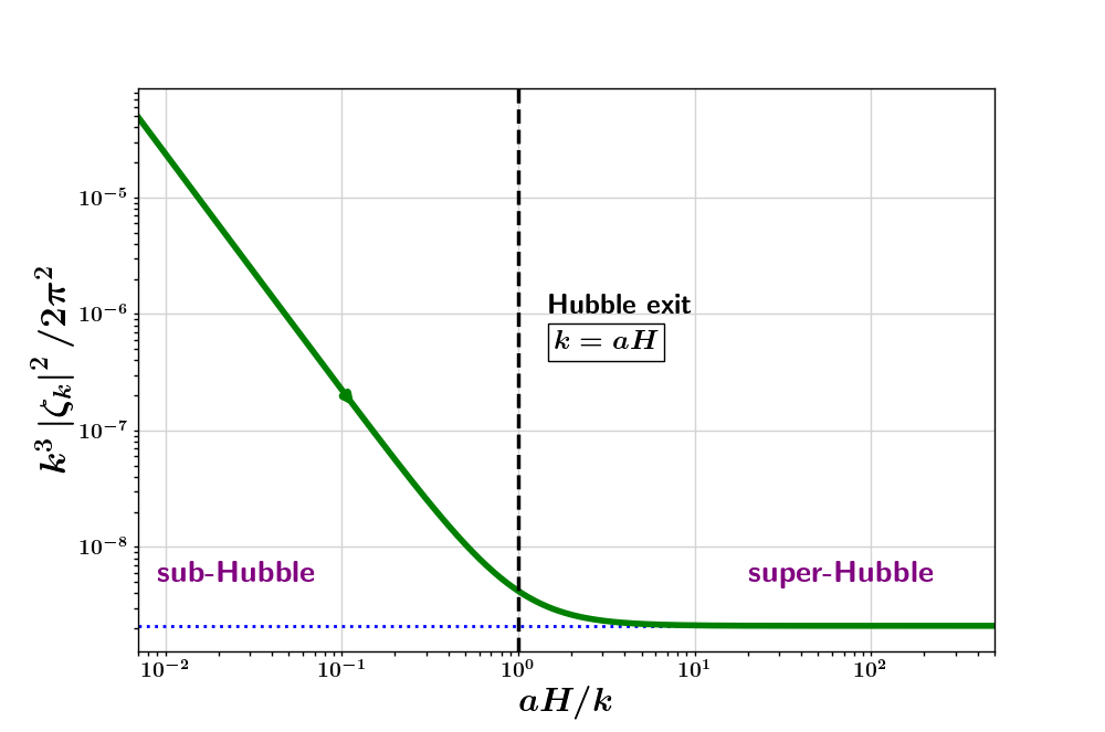
Figure 10: Evolution of the scalar power spectrum $\frac{k^{3}}{2\pi^{2}}|\zeta_{k}|^{2}$ is plotted by numerically solving Eq. (114) for a mode exiting the Hubble radius at about 60 e-folds before the end of inflation (for the Starobinsky potential given in Eq. 218). At early times when the mode is sub-Hubble, i.e. $k\gg aH$, the power decreases as ${\cal P}_{\zeta}\sim(aH)^{-2}$ as expected. After the Hubble-exit, the power freezes to a constant in the super-Hubble regime when $k\ll aH$. We note down its value after the mode-freezing as the super-Hubble scale power corresponding to that mode. Repeating the procedure for a range of scales $k$ yields us the power spectrum of scalar fluctuations. The same numerical analysis can be carried out for tensor fluctuations.

The conservation of $\zeta_{k}$ for adiabatic perturbations on super-Hubble scales is one of the most important consequences of the rapidly accelerated expansion during inflation. This allows us to translate/extrapolate the power spectra of inflationary fluctuations (at large cosmological scales) at the end of inflation through the unknown reheating history of the universe (discussed in Sec. 8), all the way until these fluctuations enter the Hubble radius closer to matter-radiation equality and recombination epochs. Thus, it enables inflation to make firm predictions about the late time structure in the universe. It is important to stress that the conservation of $\zeta_{k}$ for adiabatic perturbations on super-Hubble scales is also valid beyond Einstein’s gravity and potentially beyond linear perturbation theory, as demonstrated in Refs. [97, 98].

The aforementioned classical dynamics of $\zeta_{k}$ provides us with intuitive insights into the qualitative properties of super-Hubble scalar fluctuations during inflation. In order to quantitatively compute the power spectrum, we need to consider vacuum quantum fluctuations during inflation, for which we will treat the fields $\hat{\zeta}$ and $\hat{v}$ as quantum fields. Since the action for $\hat{v}$ in Eq. (107) is in the canonically normalized form, we will apply the method of canonical quantization discussed in Sec. 6.1 to quantize it. Working in the Heisenberg picture, we expand $\hat{v}$ in terms of creation and annihilation operators as follows:

$$\hat{v}(\tau,\vec{x})=\int\,\frac{{\rm d}^{3}\vec{k}}{(2\pi)^{3}}\,\hat{v}_{k}(\tau)\,e^{i\vec{k}.\vec{x}}=\int\,\frac{{\rm d}^{3}\vec{k}}{(2\pi)^{3}}\,\left[v_{k}(\tau)\,e^{i\vec{k}.\vec{x}}\,\hat{a}_{\vec{k}}+v^{*}_{k}(\tau)\,e^{-i\vec{k}.\vec{x}}\,\hat{a}_{\vec{k}}^{\dagger}\right]\,,$$ (116)

where the Fourier modes $\hat{v}_{k}$ are those of the one-dimensional time dependent quantum harmonic oscillators, that can be written as

$$\hat{v}_{k}(\tau)=v_{k}(\tau)\,\hat{a}_{\vec{k}}+v^{*}_{k}(\tau)\,\hat{a}_{-\vec{k}}^{\dagger}\,,$$ (117)

with $\hat{a}_{\vec{k}},\,\hat{a}_{\vec{k}}^{\dagger}$ being the annihilation and creation operators respectively, satisfying the usual commutation relations

$$\left[\hat{a}_{\vec{k}_{1}},\,\hat{a}_{\vec{k}_{2}}^{\dagger}\right]=(2\pi)^{3}\,\delta_{\rm D}^{3}\left(\vec{k}_{1}-\vec{k}_{2}\right)\,.$$ (118)

The mode functions $v_{k}(\tau)$ satisfy the Mukhanov-Sasaki Eq. (110), namely

$$v^{\prime\prime}_{k}\,+\,\left(k^{2}-\frac{z^{\prime\prime}}{z}\right)v_{k}=0\,,$$ (119)

and hence they only depend on the magnitude $k=|\vec{k}|$ of the comoving frequency.

Given a mode $k$, at sufficiently early times when it is deep in the sub-Hubble regime i.e $k\gg aH$, we can assume $v_{k}$ to be the fluctuations of a massless field in Minkowski spacetime. Consequently, we impose the Bunch-Davies vacuum initial condition [99]

$$\boxed{v_{k}\big{|}_{-k\tau\gg 1}=\frac{1}{\sqrt{2k}}\,e^{-ik\tau}}\,,$$ (120)

on each cosmologically observable mode at sufficiently early times during inflation. At this stage, it is important to point out that we will be using the results from quantum field theory(QFT) at two important places, namely: (i) in the definition of power spectrum given in Eq. (113), as discussed in Sec. 6.1, and (ii) in choosing the initial quantum vacuum which is characterised by the Bunch-Davies mode functions given in Eq. (120).

As discussed before, during inflation the comoving Hubble radius falls, causing modes to become super-Hubble i.e $k\ll aH$ and Eq. (110) dictates that $|v_{k}|\propto z$ and hence $\zeta_{k}$ approaches a constant value. By solving the Mukhanov-Sasaki equation we can estimate the dimensionless primordial power spectrum of $\zeta$ using Eq. (113). Imposing standard normalisation from QFT given in Eq. (97) and the Bunch-Davies initial conditions (120) on the general solution given in Eq. (112), we get

1. Normalisation $\Rightarrow\leavevmode\nobreak\ \leavevmode\nobreak\ |C_{1}|^{2}-|C_{2}|^{2}=1$ (where $\hbar=1$) ;

2. Bunch-Davies condition $\Rightarrow\leavevmode\nobreak\ \leavevmode\nobreak\ v_{k}(\tau)\longrightarrow\frac{1}{\sqrt{2k}}e^{-ik\tau}$ for $k|\tau|\gg 1\,,$

leading to

$$C_{1}=1,\leavevmode\nobreak\ C_{2}=0\,,$$

which then fixes the vacuum state $|0\rangle$, and yields the expression for the quasi-dS mode functions of the Mukhanov-Sasaki variable to be

$$\boxed{v_{k}(\tau)=\frac{1}{\sqrt{2k}}\left(1-\frac{i}{k\tau}\right)e^{-i\,k\tau}}\,,$$ (121)

with

$$\Rightarrow\left|v_{k}\right|^{2}=\frac{1}{2k}\,\frac{\left(1+k^{2}\tau^{2}\right)}{k^{2}\tau^{2}}\,.$$

Incorporating the Bunch-Davies initial condition imposed mode functions from Eq. (121), we obtain the scalar power spectrum, defined in Eq. ( 113), to be

$${\cal P}_{\zeta}(k)=\frac{1}{8\pi^{2}}\left(\frac{H}{m_{p}}\right)^{2}\frac{1}{\epsilon_{H}}\left[1+\left(\frac{k}{aH}\right)^{2}\right]\,,$$ (122)

which on super-Hubble scales, $k\ll aH$, is given by the (famous) expression

$$\boxed{{\cal P}_{\zeta}(k)\Big{|}_{k\ll aH}=\frac{1}{8\pi^{2}}\left(\frac{H}{m_{p}}\right)^{2}\frac{1}{\epsilon_{H}}}\leavevmode\nobreak\ ,$$ (123)

which shows that there is finite power on super-Hubble scales which depends on the Hubble parameter $H$ and the first slow-roll parameter $\epsilon_{H}$ during inflation. The scalar and tensor power spectra determined using the slow-roll approximations have been plotted in Fig. 11 for the Starobinsky potential given in Eq. (218). From Eqs. (122) and (123), it is easy to notice that the frozen value of the scalar power spectrum at late times $k\ll aH$ is half of its value at the Hubble-crossing $k=aH$, as can be seen in Fig. 10. However, since $H^{2}/\epsilon_{H}$ is almost constant during slow-roll, this implies,

$$\frac{H^{2}}{\epsilon_{H}}\bigg{|}_{k=aH}\,\simeq\,\frac{H^{2}}{\epsilon_{H}}\bigg{|}_{k\ll aH}\,,$$

we can use the corresponding values of $H$ and $\epsilon_{H}$ at the Hubble crossing of a particular mode to compute the power spectrum, as long as we are using Eq. (123), instead of Eq. (122). This is known as the Hubble-crossing formalism [100, 79].

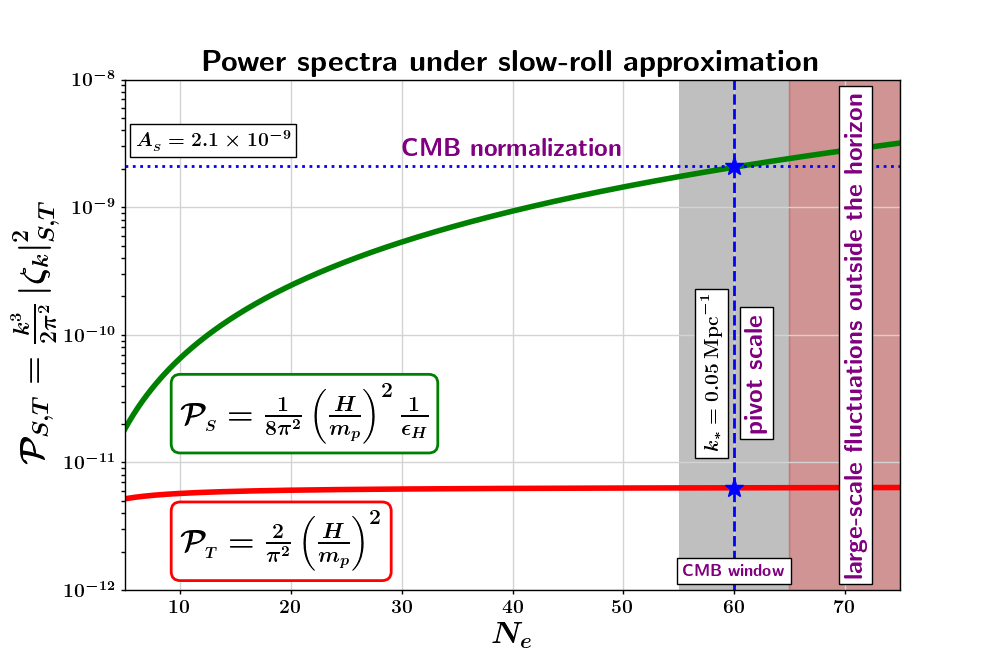
Figure 11: The power spectra of scalar and tensor quantum fluctuations (computed using the slow-roll formulae given by Eqs. (123) and (162) respectively) are shown for comoving modes exiting the Hubble radius at different number of e-folds $N_{e}$ before the end of inflation for the Starobinsky potential in Eq. (218). The CMB window (shown as the grey shaded region) corresponds to comoving modes in the range $k_{\rm CMB}\in[0.0005,0.5]\leavevmode\nobreak\ {\rm Mpc}^{-1}$ that are being probed by the current CMB missions. Fluctuations over larger scales (shown as the red shaded region) are outside the observable universe at present.

In order to compare the inflationary predictions with CMB observations, it is instructive to write the scalar power spectrum given in Eq. (123) in the form of a power-law as

$${\cal P}_{\zeta}(k)=A_{S}\left(\frac{k}{k_{*}}\right)^{n_{{}_{S}}-1}\,,$$ (124)

where, $A_{S}$ is the amplitude of scalar fluctuations at the pivot scale $k=k_{*}$. The scalar spectral index $n_{{}_{S}}-1$ is defined as

$$n_{{}_{S}}-1=\frac{{\rm d}\ln{\cal P}_{\zeta}}{{\rm d}\ln k}=\frac{{\rm d}\ln{\cal P}_{\zeta}}{{\rm d}N}\,\frac{{\rm d}N}{{\rm d}\ln k}\,,$$ (125)

which is to be computed at the Hubble-crossing $k=aH$ of a given mode. Hence we get

$$\frac{{\rm d}\ln k}{{\rm d}N}=1+\frac{{\rm d}\ln H}{{\rm d}N}=1-\epsilon_{H}\,,$$

leading to

$$\Rightarrow\frac{{\rm d}N}{{\rm d}\ln k}=\frac{1}{1-\epsilon_{H}}\simeq 1+\epsilon_{H}+{\cal O}\left(\epsilon_{H}^{2}\right)\,.$$ (126)

Similarly, from Eq. (123), we get

$$\frac{{\rm d}\ln{\cal P}_{\zeta}}{{\rm d}N}=2\,\frac{{\rm d}\ln H}{{\rm d}N}-\frac{{\rm d}\ln\epsilon_{H}}{{\rm d}N}\,,$$

which, using Eq. (71) becomes

$$\Rightarrow\frac{{\rm d}\ln{\cal P}_{\zeta}}{{\rm d}N}=2\,\eta_{H}-4\,\epsilon_{H}\,.$$ (127)

Incorporating Eqs. (126) and (127) into Eq. (125) we obtain the expression for the scalar spectral index $n_{{}_{S}}-1$ to be

$$\boxed{n_{{}_{S}}-1=2\,\eta_{H}-4\,\epsilon_{H}}\,.$$ (128)

Since $\epsilon_{H},\,|\eta_{H}|\ll 1$ during slow-roll inflation, Eq. (128) shows that $n_{{}_{S}}-1\simeq 0$, implying the power spectrum is almost scale-invariant with a tiny spectral tilt. It is possible that in some specific case, the inflationary dynamics yields $\eta_{H}=2\epsilon_{H}$, leading to an exact scale-invariant/Harrison-Zeldovich power spectrum with $n_{{}_{S}}=1$. However, this will require a particular fined tuned functional form of the potential $V(\phi)$, as shown in Ref. [101].

This is in sharp contrast to the quantum fluctuations of a massless free scalar field in Minkowski space for which the mode functions are given by

$$\boxed{v_{k}^{M}(t)=\frac{1}{\sqrt{2k}}e^{-ikt}}\,.$$ (129)

Hence the power spectrum is given by

$$\boxed{{\cal P}_{M}(k)=\left(\frac{k}{2\pi}\right)^{2}}\leavevmode\nobreak\ ,$$ (130)

which has a prominent blue tilt ${\cal P}_{M}(k)\propto\left(\frac{k}{2\pi}\right)^{2}$ on all scales, because of which the power is strongly suppressed on large scales and has negligible macroscopic consequence.

The key difference between inflationary fluctuations and fluctuations in Minkowski spacetime is the presence of the tachyonic mass term in Eq. (110), which forces the mode functions $v_{k}$ to grow linearly with scale factor, thus making sure that $\zeta_{k}$ is conserved on super-Hubble scales. In fact the growth/instability of $v_{k}$ can be understood from the fact that Eq. (110) describes an inverted oscillator at late times, when $k^{2}\tau^{2}\ll 1$, featuring a maximum at the centre [102] as shown in Fig. 12. Accordingly, $\zeta_{k}$ behaves like an over-damped oscillator whose damping term increases quickly/non-adiabatically as the mode becomes super-Hubble. To see this qualitatively, let us consider the effective frequency/mass term of the Mukhanov-Sasaki variable, namely

$$\Omega_{v}^{2}(k,\tau) = k^{2}+{\cal M}_{\rm eff}^{2}(\tau)=k^{2}-\frac{2}{\tau^{2}}\,;$$ (131)

$$\Omega_{v}^{{}^{\prime}}(k,\tau) = \frac{2}{\tau^{3}\,\Omega_{v}}\,,$$ (132)

for which, one obtains

$$\bigg{|}\frac{\Omega^{\prime}}{\Omega^{2}}\bigg{|}=\bigg{|}\frac{2}{\left(k^{2}\tau^{2}-2\right)^{3/2}}\bigg{|}\,.$$ (133)

The above expression demonstrates that $\big{|}\frac{\Omega^{\prime}}{\Omega^{2}}\big{|}\geq 1$ when $-k\tau\leq 2$, indicating violation of adiabaticity, as the mode approaches the Hubble radius, generating large excitations of the $\hat{v}$ quanta. The effective mass term of the $\hat{v}$ field becomes tachyonic after Hubble crossing. Hence, the initial Bunch-Davies type vacuum fluctuations appear to be in a highly excited state from the point of view of the late time Hamiltonian when the modes are super-Hubble. In the following, we will explicitly quantify the above qualitative arguments. Since this excited state corresponds to large occupation number of particles, the super-Hubble quantum fluctuations can be considered as classical in this regard [103, 102]. The issue of quantum-to-classical transition is rather complex and is a topic of intense investigation (see Refs. [104, 105, 106, 107, 108, 109, 110, 111, 112, 113, 114, 115, 116, 117, 118]).

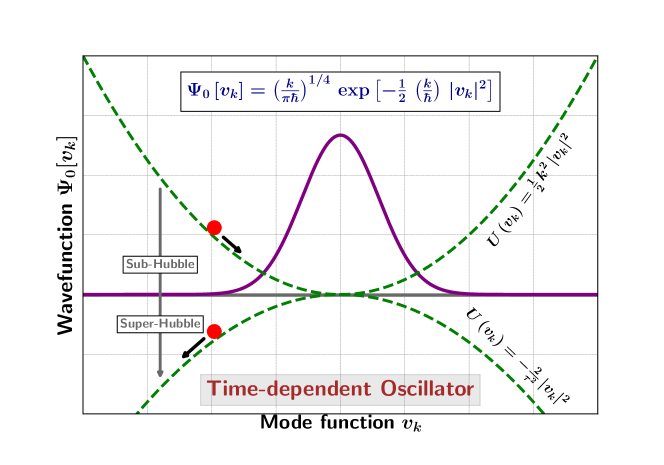
Figure 12: The time-dependent effective potential and the ground state wave function are plotted in green and purple respectively for a harmonic oscillator with a time dependent frequency as a representative of the Mukhanov-Sasaki mode functions $v_{k}$, as described by Eq. (119).

The quadratic action for $\hat{\zeta}$ in Eq. (102) can be written in terms of the Fourier modes by proceeding as follows. Incorporating the Fourier decomposition of $\hat{\zeta}$

$$\hat{\zeta}(\tau,\vec{x})=\int\frac{{\rm d}^{3}\vec{k}}{(2\pi)^{3}}\leavevmode\nobreak\ \hat{\zeta}_{\vec{k}}(\tau)\leavevmode\nobreak\ e^{i\,\vec{k}.\vec{x}}$$

into the action in Eq. (102), we get

$$S^{(2)}[\hat{\zeta}(\tau,\vec{x})]=\frac{1}{2}\int{\rm d}\tau\,z^{2}\int\frac{{\rm d}^{3}\vec{k}_{1}}{(2\pi)^{3}}\int\frac{{\rm d}^{3}\vec{k}_{2}}{(2\pi)^{3}}\int{\rm d}^{3}\vec{x}\,e^{i\left(\vec{k}_{1}+\vec{k}_{2}\right).\vec{x}}\left[\hat{\zeta}^{\prime}_{\vec{k}_{1}}\hat{\zeta}^{\prime}_{\vec{k}_{2}}-\left(i\,\vec{k}_{1}\right).\left(i\,\vec{k}_{2}\right)\hat{\zeta}_{\vec{k}_{1}}\hat{\zeta}_{\vec{k}_{2}}\right]\,.$$

Using the definition of Dirac delta function

$$\delta_{D}^{(3)}(\vec{k}_{1}+\vec{k}_{2})=\frac{1}{(2\pi)^{3}}\,\int{\rm d}^{3}\vec{x}\,e^{i\left(\vec{k}_{1}+\vec{k}_{2}\right).\vec{x}}\,,$$ (134)

we obtain the expression for the quadratic action of $\hat{\zeta}$ to be

$$S^{(2)}[\hat{\zeta}]=\frac{1}{2}\int{\rm d}\tau\int\frac{{\rm d}^{3}\vec{k}}{(2\pi)^{3}}\,z^{2}\left[\left(\hat{\zeta}_{k}^{\prime}\right)^{2}-k^{2}\,\hat{\zeta}_{k}^{2}\right]\,.$$ (135)

Similarly the quadratic action for the Mukhanov-Sasaki variable $\hat{v}$ from Eq. (107) becomes

$$S^{(2)}[\hat{v}]=\frac{1}{2}\int{\rm d}\tau\int\frac{{\rm d}^{3}\vec{k}}{(2\pi)^{3}}\left[\left(\hat{v}_{k}^{\prime}\right)^{2}-\left(k^{2}+{\cal M}_{\rm eff}^{2}\right)\hat{v}_{k}^{2}\right]\,.$$ (136)

From the above actions written in terms of Fourier modes, we can compute the vacuum expectation values of any relevant physical quantity associated with the quantum field $\hat{v}$, since we have fixed the vacuum $|0\rangle$ w.r.t to the Bunch-Davies condition imposed mode functions given in Eq. (121), re-written as

$$v_{k}(\tau) = \frac{1}{\sqrt{2k}}\left(1-\frac{i}{k\tau}\right)e^{-i\,k\tau}\,;$$ (137)

$$\zeta_{k}(\tau) = \frac{-\tau}{\sqrt{2k}}\left(\frac{H}{m_{p}}\right)\,\frac{1}{\sqrt{2\epsilon_{H}}}\left(1-\frac{i}{k\tau}\right)e^{-i\,k\tau}\,.$$ (138)

The conjugate momentum of the Mukhanov-Sasaki field is $\hat{\Pi}_{v}=\hat{v}^{\prime}$, while its Lagrangian density is given by

$${\cal L}_{v}^{(2)}=\frac{1}{2}\left[\left(\hat{v}^{\prime}\right)^{2}-\left(\partial_{i}\hat{v}\right)^{2}-{\cal M}_{\rm eff}^{2}\hat{v}^{2}\right]\,.$$

Hence the Hamiltonian corresponding to the Mukhanov-Sasaki field is

$$\hat{H}_{v}^{(2)}\equiv\int{\rm d}^{3}\vec{x}\,\left(\hat{v}\,\hat{\Pi}_{v}-{\cal L}^{(2)}\right)=\frac{1}{2}\int{\rm d}^{3}\vec{x}\,\left[\hat{\Pi}_{v}^{2}+\left(\partial_{i}\hat{v}\right)^{2}+{\cal M}_{\rm eff}^{2}\hat{v}^{2}\right]\,,$$ (139)

which takes the following form in terms of Fourier modes $\hat{v}_{k}$:

$$\hat{H}_{v}^{(2)}=\frac{1}{2}\int\frac{{\rm d}^{3}\vec{k}}{(2\pi)^{3}}\left[\left(\hat{v}_{k}^{\prime}\right)^{2}+\left(k^{2}+{\cal M}_{\rm eff}^{2}\right)\hat{v}_{k}^{2}\right]\,.$$ (140)

Expanding the quantum field $\hat{v}$ and its momentum $\hat{\Pi}_{v}$ in terms of creation and annihilation operators, as given in Eq. (116), we obtain

$$\hat{v}_{k}(\tau) = v_{k}(\tau)\,\hat{a}_{\vec{k}}+v_{k}^{\ast}(\tau)\,\hat{a}_{-\vec{k}}^{\dagger}\,;$$ (141)

$$\hat{\Pi}_{v}(\tau) = v^{\prime}_{k}(\tau)\,\hat{a}_{\vec{k}}+v_{k}^{\prime\ast}(\tau)\,\hat{a}_{-\vec{k}}^{\dagger}\,.$$ (142)

Using the above Eqs. (141), (142) in Eq. (140), we obtain

$$\hat{H}_{v}^{(2)}=\frac{1}{2}\int\frac{{\rm d}^{3}\vec{k}}{(2\pi)^{3}}\left[\left(\left(v_{k}^{\prime}\right)^{2}+\Omega_{k}^{2}v_{k}^{2}\right)\hat{a}_{\vec{k}}\hat{a}_{\vec{k}}+\left(\left(v_{k}^{\prime\ast}\right)^{2}+\Omega_{k}^{2}v_{k}^{\ast\,2}\right)\hat{a}_{-\vec{k}}^{\dagger}\hat{a}_{-\vec{k}}^{\dagger}\right.$$

$$\left.+\left(|v_{k}^{\prime}|^{2}+\Omega_{k}^{2}|v_{k}|^{2}\right)\left(\hat{a}_{\vec{k}}\hat{a}_{-\vec{k}}^{\dagger}+\hat{a}_{-\vec{k}}^{\dagger}\hat{a}_{\vec{k}}\right)\right],$$

where the time dependent frequency is given by

$$\Omega_{k}^{2}=k^{2}+{\cal M}_{\rm eff}^{2}(\tau)=k^{2}-\frac{2}{\tau^{2}}\,.$$

Using the commutation relation from Eq. (118), we get

$$\hat{a}_{\vec{k}}\hat{a}_{-\vec{k}}^{\dagger}=(2\pi)^{3}\,\delta_{D}^{(3)}(0)+\hat{a}_{-\vec{k}}^{\dagger}\hat{a}_{\vec{k}}\,,$$

which leads to

$$\hat{H}_{v}^{(2)}=\frac{1}{2}\int\frac{{\rm d}^{3}\vec{k}}{(2\pi)^{3}}\left[\left(\left(v_{k}^{\prime}\right)^{2}+\Omega_{k}^{2}v_{k}^{2}\right)\hat{a}_{\vec{k}}\hat{a}_{\vec{k}}\,+\,\left(\left(v_{k}^{\prime\ast}\right)^{2}+\Omega_{k}^{2}v_{k}^{\ast\,2}\right)\hat{a}_{-\vec{k}}^{\dagger}\hat{a}_{-\vec{k}}^{\dagger}\right.$$

$$\left.+\left(|v_{k}^{\prime}|^{2}+\Omega_{k}^{2}|v_{k}|^{2}\right)\left(2\hat{a}_{-\vec{k}}^{\dagger}\hat{a}_{\vec{k}}+(2\pi)^{3}\delta_{D}^{(3)}(0)\right)\right]\,.$$ (143)

The energy of the quantum field is given by the vacuum expectation value of the Hamiltonian, namely,

$$E_{v}\equiv\langle\,0\,|\,\hat{H}_{v}^{(2)}\,|\,0\,\rangle=\frac{1}{2}\,(2\pi)^{3}\,\delta_{D}^{(3)}(0)\,\int\frac{{\rm d}^{3}\vec{k}}{(2\pi)^{3}}\,\left[\,|v_{k}^{\prime}|^{2}+\Omega_{k}^{2}|v_{k}|^{2}\,\right]\,.$$ (144)

The appearance of the Dirac delta function indicates that formally the total vacuum energy of the quantum field is divergent, as expected. A better physical quantity to compute is the vacuum energy density, $\rho_{v}$. Noting that

$$(2\pi)^{3}\delta^{(3)}(0)=\lim_{|\vec{k}|\to 0}\,\int\,{\rm d}^{3}\vec{x}\,e^{i\,\vec{k}.\vec{x}}=\int\,{\rm d}^{3}\vec{x}\,,$$

the vacuum energy density can be obtained from Eq. (144) to be

$$\rho_{v}=\frac{1}{2}\,\int\frac{{\rm d}^{3}\vec{k}}{(2\pi)^{3}}\,\left[\,|v_{k}^{\prime}|^{2}+\Omega_{k}^{2}\,|v_{k}|^{2}\,\right]\,.$$ (145)

At this stage, it is important to obtain simplified expressions for $v_{k}$ and $v_{k}^{\prime}$, starting from Eq. (137), as

$$v_{k}(\tau) =\frac{1}{\sqrt{2k}}\left(1-\frac{i}{k\tau}\right)e^{-i\,k\tau}\leavevmode\nobreak\ \Rightarrow\leavevmode\nobreak\ |v_{k}(\tau)|^{2}=\frac{1}{2k}\left(1+\frac{1}{k^{2}\tau^{2}}\right)\,;$$ (146)

$$v_{k}^{\prime}(\tau) =\frac{1}{\sqrt{2k}}\,\frac{1}{\tau}\,\left[-1+i\left(\frac{1}{k\tau}-k\tau\right)\right]e^{-i\,k\tau}\leavevmode\nobreak\ \Rightarrow\leavevmode\nobreak\ |v_{k}^{\prime}(\tau)|^{2}=\frac{k}{2}\left(1-\frac{1}{k^{2}\tau^{2}}+\frac{1}{k^{4}\tau^{4}}\right)\,,$$ (147)

which can be used to compute the integrand of Eq. (145) to be

$$|v_{k}^{\prime}|^{2}+\Omega_{k}^{2}|v_{k}|^{2}\simeq|v_{k}^{\prime}|^{2}+\left(k^{2}-\frac{2}{\tau^{2}}\right)|v_{k}|^{2}=\frac{k}{2}\left(2-\frac{2}{k^{2}\tau^{2}}-\frac{1}{k^{4}\tau^{4}}\right)\,.$$ (148)

It is instructive to obtain the following sub-Hubble and super-Hubble limits of the above expression:

$$|v_{k}^{\prime}|^{2}+\Omega_{k}^{2}|v_{k}|^{2}\bigg{|}_{-k\tau\to\infty} = k\,;$$ (149)

$$|v_{k}^{\prime}|^{2}+\Omega_{k}^{2}|v_{k}|^{2}\bigg{|}_{-k\tau\to 0} = -\frac{k}{2}\left(\frac{1}{k^{4}\tau^{4}}\right)\,.$$ (150)

Incorporating the expression in Eq. (150) into Eq. (145), we obtain the energy density of the super-Hubble (IR) part of the $\hat{v}$ field to be

$$\rho_{v}\big{|}_{\rm IR}(\tau)=-\frac{1}{2}\int_{k_{\rm IR}}^{-1/\tau}\frac{{\rm d}^{3}\vec{k}}{(2\pi)^{3}}\leavevmode\nobreak\ \frac{k}{2}\,\left(\frac{1}{k^{4}\tau^{4}}\right)=-\frac{1}{4\pi^{2}}\frac{1}{\tau^{4}}\int_{k_{\rm IR}}^{-1/\tau}{\rm d}\,\left(\ln k\right)=-\frac{1}{4\pi^{2}}\frac{1}{\tau^{4}}\ln\left(\frac{-1}{k_{\rm IR}\tau}\right)\,,$$ (151)

where $k_{\rm IR}$ is a cut-off introduced to regulate the IR divergence (since inflation may have a beginning [119], $k_{\rm IR}$ corresponds to the comoving mode making its Hubble-exit at the beginning of inflation). Eq. (151) demonstrates that the energy density of the super-Hubble part of $\hat{v}$ diverges at late times, $-\tau\to 0$, which can be attributed to the fact that the effective mass term is tachyonic, as described previously in Fig. 12 with the analogy of an inverted oscillator. (Note that the energy density corresponding to the sub-Hubble (UV) part of the $\hat{v}$ field in Eq. (149) leads to the usual UV divergence associated with quantum fluctuations in Minkowski spacetime.)

Similarly we compute the expectation value of the occupation number density of particles of a given mode $k$ to be

$$\langle\,0\,|\,\hat{n}_{v}(k)\,|\,0\,\rangle\equiv\frac{1}{2}\,\Big{|}\frac{|v_{k}^{\prime}|^{2}+\Omega_{k}^{2}|v_{k}|^{2}}{k}\Big{|}_{-k\tau\to 0}-\frac{1}{2}\simeq\frac{1}{4}\,\left(\frac{-1}{k\tau}\right)^{4}\to\infty,$$ (152)

which diverges, indicating abundant excitations of $\hat{v}$ quanta, as discussed before. The corresponding energy density and particle number density for the $\hat{\zeta}$ field can be obtained by $\hat{\zeta}=\hat{v}/(am_{p}\sqrt{2\epsilon_{H}})$. Accordingly, the finite and frozen power spectrum of $\hat{\zeta}$ on super-Hubble scales can be justified in this Heisenberg picture. Note that similar arguments are also applicable for the tensor-type fluctuations discussed in Sec. 6.3. See App. F for a discussion on the quantum fluctuations of a massive scalar field in de Sitter spacetime and their relation to the inflationary scalar fluctuations.

Before concluding the treatment of scalar fluctuations, let us stress that the computation of the inflationary scalar power spectrum given in Eq. (123) is one of the key achievements of modern theoretical cosmology. This is certainly one of the most important applications of quantum field theory to curved spacetime in physics, generating the seeds for the large-scale cosmological structure in the universe. These results were first obtained in the early 1980s around the time of the famous Nuffield conference organised by Stephen Hawking and colleagues (see Ref. [121]) and were published in Refs. [10, 11, 12, 13]. For a historical account of the subject, see the popular Ref. [122].

6.3 Tensor quantum fluctuations during inflation

The gauge-invariant tensor fluctuations $h_{ij}(\tau,\vec{x})$ during inflation are described by the quadratic action [85, 91]

$$S^{(2)}[h_{ij}]=\frac{1}{2}\int{\rm d}\tau\leavevmode\nobreak\ {\rm d}^{3}\vec{x}\leavevmode\nobreak\ \left(\frac{am_{p}}{2}\right)^{2}\left[h_{ij}^{\prime 2}-(\partial_{l}h_{ij})^{2}\right]\,,$$ (153)

where the transverse and traceless tensor field $h_{ij}(\tau,\vec{x})$ satisfies

$$\partial^{i}\,h_{ij}=0\leavevmode\nobreak\ \leavevmode\nobreak\ \text{(transverse)}\,;\quad h_{i}^{i}=0\leavevmode\nobreak\ \leavevmode\nobreak\ \text{(traceless)}\,,$$ (154)

and can be decomposed into its two orthogonal polarization components,

$$h_{ij}(\tau,\vec{x}) =\frac{1}{\sqrt{2}}\begin{bmatrix}h_{+}&h_{\times}&0\\ h_{\times}&-h_{+}&0\\ 0&0&0\end{bmatrix}=\frac{1}{\sqrt{2}}\begin{bmatrix}1&0&0\\ 0&-1&0\\ 0&0&0\end{bmatrix}h_{+}(\tau,\vec{x})+\frac{1}{\sqrt{2}}\begin{bmatrix}0&1&0\\ 1&0&0\\ 0&0&0\end{bmatrix}h_{\times}(\tau,\vec{x})$$ (155)

$$=\frac{1}{\sqrt{2}}\leavevmode\nobreak\ \epsilon^{+}_{ij}\,h_{+}(\tau,\vec{x})+\frac{1}{\sqrt{2}}\leavevmode\nobreak\ \epsilon^{\times}_{ij}\,h_{\times}(\tau,\vec{x})\,,$$ (156)

with $\epsilon^{\lambda}_{ij}\epsilon^{ij\,\lambda^{\prime}}=2\delta^{\lambda\lambda^{\prime}};\leavevmode\nobreak\ \lambda=\{+,\times\}$. The action can be rewritten as

$$S^{(2)}[h_{+},\,h_{\times}]=\frac{1}{2}\int{\rm d}\tau\leavevmode\nobreak\ {\rm d}^{3}\vec{x}\leavevmode\nobreak\ \left(\frac{am_{p}}{2}\right)^{2}\,\sum_{\lambda=+,\times}\,\left[({h_{\lambda}}^{\prime})^{2}-(\partial_{l}h_{\lambda})^{2}\right]\,.$$ (157)

We define the two Mukhanov-Sasaki variables for the tensor perturbations to be

$$v_{\lambda}=\left(\frac{am_{p}}{2}\right)h_{\lambda}\,,$$ (158)

in terms of which the action becomes

$$\boxed{\,S^{(2)}[v_{+},\,v_{\times}]=\frac{1}{2}\int{\rm d}\tau\leavevmode\nobreak\ {\rm d}^{3}\vec{x}\leavevmode\nobreak\ \,\sum_{\lambda=+,\times}\,\left[({v_{\lambda}}^{\prime})^{2}-(\partial_{i}v_{\lambda})^{2}+\frac{a^{\prime\prime}}{a}\,{v_{\lambda}}^{2}\right]\,}\,,$$ (159)

which is equivalent to the action of two massless scalar fields in de Sitter spacetime, as can be inferred by comparing this with Eq. (107). The full power spectrum of tensor fluctuations is defined by

$${\cal P}_{T}(k) =\frac{k^{3}}{2\pi^{2}}\left(\absolutevalue{h_{+}}^{2}+\absolutevalue{h_{\times}}^{2}\right)=\frac{k^{3}}{2\pi^{2}}\left(\frac{2}{am_{p}}\right)^{2}\left(\absolutevalue{v_{+}}^{2}+\absolutevalue{v_{\times}}^{2}\right)\,.$$ (160)

Borrowing the result from Eq. (121) in Sec. (6.2), we obtain

$${\cal P}_{T}(k)=\frac{2}{\pi^{2}}\left(\frac{H}{m_{p}}\right)^{2}\left(1+k^{2}\tau^{2}\right)\,,$$ (161)

which on super-Hubble scales $|k\tau|\to 0$ takes the form

$$\boxed{{\cal P}_{T}(k)\Big{|}_{k\ll aH}=\frac{2}{\pi^{2}}\left(\frac{H}{m_{p}}\right)^{2}}\,.$$ (162)

The tensor power spectrum only depends upon the Hubble parameter during inflation, and hence encodes direct information about the energy scale of inflation. In contrast, the scalar power spectrum in Eq. (123) depends both on the Hubble parameter $H$ and the first slow-roll parameter $\epsilon_{H}$, as stressed before. The tensor power spectrum in de Sitter spacetime was originally computed by Starobinsky in his pioneering work [18] in 1979, a year before the inception of the inflationary hypothesis.

Similar to the scalar power spectrum in Eq. (124), we can also write the tensor power spectrum as a power law, that is,

$${\cal P}_{T}(k)=A_{T}\left(\frac{k}{k_{*}}\right)^{n_{{}_{T}}}$$ (163)

where $A_{T}$ is the amplitude of the tensor modes at the pivot scale $k_{*}$ which is chosen to be $k_{*}=0.05\,\rm Mpc^{-1}$ and $n_{{}_{T}}$ is the tensor spectral index. An important quantity is the tensor-to-scalar ratio which is defined as,

$$r=\frac{A_{T}}{A_{S}}=\frac{{\cal P}_{T}(k_{*})}{{\cal P}_{\zeta}(k_{*})}.$$ (164)

Using Eqs. (123) and (162), we have

$$r=16\,\epsilon_{H}$$ (165)

$$n_{{}_{T}}=-2\,\epsilon_{H}$$ (166)

Thus, a consistency relation can be established between the tensor spectral index and the tensor-to-scalar ratio as,

$$r=-8\,n_{{}_{T}}\,,$$ (167)

which can be used as a smoking gun test of the single field slow-roll inflationary paradigm.

By this stage, a careful reader must have noticed that the scalar spectral index is denoted as $n_{{}_{S}}-1$, while the tensor spectral index is denoted as $n_{{}_{T}}$. Such a difference in the notation is an unfortunate historical artifact. Since scale-invariance is an approximate symmetry during inflation, we should have denoted the scalar spectral index by $n_{{}_{S}}$, where $|n_{{}_{S}}|\ll 1$ is a small number. In fact, we had originally intended to use this improved notation throughout these lecture notes. However, this might have created potential confusion for the reader since most other sources use $n_{{}_{S}}-1$. For this reason, we have (reluctantly) reverted to use the standard $n_{{}_{S}}-1$ notation for the scalar spectral index. Furthermore, notice that in Fig. 14, we labelled the $X$-axis as scalar spectral index, although we plot $n_{{}_{S}}$, rather than $n_{{}_{S}}-1$. Again, we have reluctantly given in to such a convention in order to be consistent with Fig. 8 of Ref. [2].

Before moving on to study the dynamics of different popular inflationary models, it is important to remind the readers that we are working in natural units, where $\hbar,\,c=1$. Hence they do not appear in the expressions for the power spectra of quantum fluctuations in Eqs. (123) and (162). Putting $\hbar$ and $c$ back into the expressions for power spectra, we obtain

$${\cal P}_{\zeta}(k)\Big{|}_{k\ll aH} = \frac{1}{8\pi^{2}}\,\left(\frac{\hbar}{c^{5}}\right)\,\left(\frac{H}{m_{p}}\right)^{2}\,\frac{1}{\epsilon_{H}}\,,$$ (168)

$${\cal P}_{T}(k)\Big{|}_{k\ll aH} = \frac{2}{\pi^{2}}\,\left(\frac{\hbar}{c^{5}}\right)\,\left(\frac{H}{m_{p}}\right)^{2}\,.$$ (169)

6.4 Beyond linear perturbation theory: primordial non-Gaussianity

In Secs. 6.2 and 6.3, we computed the power spectra corresponding to the two-point auto-correlator of the scalar and tensor fluctuations at linear order in perturbation theory, using the quadratic actions given by Eqs. (102) and (153). At linear order, the scalar and tensor fluctuations behave like free (non-interacting) quantum fields and hence their wave functions are Gaussian [123]. Therefore, the computation of their skewness coming from the three-point (and higher odd-point) correlators using the quadratic action yields vanishing non-Gaussianity.

Even though the inflationary fluctuations are highly Gaussian, we expect a minimal amount of non-Gaussianity to be present because – (i) Einstein’s field equations are inherently non-linear, and (ii) the inflaton’s self-interaction potential $V(\phi)$ is usually not quadratic. In order to compute them carefully, we need to move beyond the free (quadratic) actions and work with the interaction action (85). In the following, we briefly mention some of the key results on primordial non-Gaussianity in the context of single field slow-roll inflation.

A systematic computation of primordial non-Gaussianity using the standard techniques of interacting QFT, known as the In-In formalism, was carried out in a pioneering work in Ref. [85]. For example, using the cubic order action, we can compute the (interacting) vacuum expectation value of the bispectrum ${\cal B}_{\zeta}\left(k_{1},k_{2},k_{3}\right)$, defined as

$$\langle\,\zeta_{\vec{k}_{1}}\,\zeta_{\vec{k}_{2}}\,\zeta_{\vec{k}_{3}}\,\rangle=(2\pi)^{3}\,\left(\frac{2\pi^{2}}{k_{1}\,k_{2}\,k_{3}}\right)^{2}\,{\cal B}_{\zeta}\left(k_{1},\,k_{2},\,k_{3}\right)\,\delta_{D}^{3}\left(\vec{k}_{1}+\vec{k}_{2}+\vec{k}_{3}\right)\,,$$ (170)

where the appearance of the Dirac delta function is a manifestation of the translational invariance (homogeneity) of space during inflation, namely $\vec{k}_{1}+\vec{k}_{2}+\vec{k}_{3}=0$ which form a closed triangle of vectors. This also indicates that the magnitude of the bispectrum depends on the shape of this triangle. In particular, in the squeezed limit where one of the modes ($k_{1}$) is long and becomes super-Hubble very early compared to the other two, i.e. $k_{1}\,\ll\,k_{2},\,k_{3}$, the bispectrum takes the form [85, 124]

$$\boxed{{\cal B}_{\zeta}\left(k_{1},\,k_{2},\,k_{3}\right)\big{|}_{k_{1}\,\ll\,k_{2},k_{3}}\leavevmode\nobreak\ =\leavevmode\nobreak\ \left(1-n_{{}_{S}}\right){\cal P}_{\zeta}(k_{2}){\cal P}_{\zeta}(k_{3})}\,,$$ (171)

which is known as the (Maldacena) single field consistency relation for the bispectrum. Since $1-n_{{}_{S}}\ll 1$, the bispectrum is predicted to be very small (although necessarily non-zero) in the squeezed limit.

The relative strength of the bispectrum is usually defined in the equilateral configuration with $k_{1}=k_{2}=k_{3}=k$ as [91]

$$f_{\rm NL}(k)=\frac{5}{18}\,\frac{{\cal B}_{\zeta}\left(k,\,k,\,k\right)}{{\cal P}_{\zeta}^{2}(k)}\,,$$ (172)

which is a measure of the fractional non-linearity present in the scalar fluctuations. Note that the factor $5/18$ is again an artifact of historical notation. The latest CMB observations [64] are consistent with $f_{\rm NL}=0$, establishing the highly Gaussian nature of primordial fluctuations and providing further support for the single field inflationary paradigm. In parallel with the bispectrum of the scalar fluctuations $\zeta$, one can also study the bispectrum of tensor fluctuations $h_{ij}$, as well as the 3-point cross-correlation between the two. Additionally, one can also compute the trispectrum, corresponding to the four-point correlator, of the scalar and tensor fluctuations.

The dynamics of primordial interactions during inflation are encoded in the properties of primordial non-Gaussianity, which can be inferred from the future CMB and LSS missions. Since inflation was supposed to have occurred at ultra-high energy scales, the branch of early universe cosmology that studies the structure of higher point correlators has been termed as ‘cosmological collider physics’ [125]. A significant improvement in the sensitivity of observational cosmology is anticipated in the coming few decades, especially in the context of galaxy clustering and $21\leavevmode\nobreak\ {\rm cm}$ intensity fluctuations, which will provide crucial constraints on primordial non-Gaussianity. Since our treatment of inflationary non-Gaussianity was very minimal, we refer the readers to Refs. [124, 126, 127, 128, 129, 130] for a detailed analysis on the subject.

6.5 Post-inflationary evolution of primordial fluctuations

In the preceding subsections, we computed the primordial scalar and tensor power spectra on super-Hubble scales from inflation which serve as initial seed fluctuations for the post-inflationary universe. In the following, we briefly discuss the evolution of primordial scalar and tensor fluctuations upon their Hubble-entry in the post-inflationary epochs. We begin with scalar fluctuations, which induce temperature and density fluctuations in the CMB, and later seed the large scale structure of the universe. We then move on to discuss the evolution of tensor fluctuations which propagate as primordial GWs and constitute a stochastic GW background at the present epoch.

6.5.1 Evolution of scalar fluctuations after inflation

After the end of inflation, the super-Hubble comoving curvature perturbations $\zeta_{k}$ begin to re-enter the Hubble radius when their comoving wavenumber becomes $k=aH$. Upon their Hubble-entry they begin to oscillate and evolve with time. They subsequently induce the observed temperature anisotropies of the CMB, which ultimately leads to the large scale clustering of galaxies in the universe and the formation of the cosmic web.

In the context of the CMB, the primary observable is the two-point auto-correlator of temperature fluctuations $\delta T/\bar{T}$ along two different directions $\hat{n}_{1},\,\hat{n}_{2}$ (unit vectors) in the sky, separated by an angle $\cos{\theta}=\hat{n}_{1}.\hat{n}_{2}$. The angular power spectrum ${\cal C}_{l}^{\rm TT}$ can be conveniently defined by expanding the temperature auto-correlator in terms of spherical harmonics as

$$\left\langle\,\frac{\delta T(\hat{n}_{1})}{\bar{T}}\,\frac{\delta T(\hat{n}_{2})}{\bar{T}}\,\right\rangle\Bigg{|}_{\tau_{\rm CMB}}=\sum_{l}\,\left(\frac{2l+1}{4\pi}\right)\,{\cal C}_{l}^{\rm TT}(\tau_{\rm CMB})\,\mathbb{P}_{l}(\cos{\theta})\,,$$ (173)

where $\mathbb{P}_{l}(\cos{\theta})$ are the Legendre polynomials [131]. The angular power spectrum ${\cal C}_{l}^{\rm TT}$ of the CMB temperature fluctuations can be related to the primordial power spectrum of comoving curvature fluctuations $\zeta$ via [91]

$$\boxed{\,C_{l}^{\rm TT}(\tau_{\rm CMB})=\frac{4\pi}{(2l+1)^{2}}\,\int{\rm d}\ln{k}\leavevmode\nobreak\ {\cal T}_{l}^{2}(k,\tau_{\rm CMB})\,{\cal P}_{\zeta}(k)\,}\,,$$ (174)

where the transfer function ${\cal T}_{l}(k,\tau_{\rm CMB})$ encapsulates the evolution of $\zeta_{k}$ starting from the epoch of its Hubble-entry until recombination, followed by a projection onto the CMB sky. By correctly computing the transfer function using linear perturbation theory in the post-inflationary universe, one can determine ${\cal C}_{l}^{\rm TT}$. Note that the angular power spectrum is sensitive to both the initial primordial fluctuations and the subsequent evolution of the universe until the present epoch, when the CMB observations are made. Thus, it contains crucial information about both the early and late universe. Apart from temperature fluctuations, one can also study the fluctuations in the polarisation of the CMB, which captures information about both scalar and tensor fluctuations in the early universe. The latest CMB observations by the Planck mission and BICEP/Keck collaboration have imposed stringent constraints on the primordial scalar and tensor fluctuations, which we discuss in Sec. 7.1.

The physics of CMB fluctuations as well as the formation of the LSS of the universe are two of the most important fields of research in cosmology. We will not elaborate further on this topic in these lecture notes since it requires a larger dedicated space, but rather we direct the interested readers to Refs. [132, 33, 35, 91].

6.5.2 Evolution of tensor fluctuations after inflation

The primordial tensor modes discussed in Sec. 6.3, which become super-Hubble during inflation, make their Hubble-entry at late times when $k=aH$, manifesting themselves as stochastic GWs [18, 22, 133]. The physical frequency of these stochastic GWs at the present epoch is given by

$$f=\frac{1}{2\pi}\left(\frac{k}{a_{0}}\right)=\frac{1}{2\pi}\left(\frac{a}{a_{0}}\right)H\leavevmode\nobreak\ ,$$ (175)

where $a$, $H$ correspond to the scale factor and Hubble parameter of the universe during the epoch when the corresponding tensor mode made its Hubble-entry. The characteristic frequencies of the relic GWs that become sub-Hubble prior to matter-radiation equality are large enough to enable them to be detected by GW observatories in the near future, such as the Laser Interferometer Gravitational-Wave Observatory (LIGO) [134], Laser Interferometer Space Antenna (LISA) [135], Big Bang Observer (BBO) [136] and Pulsar Timing Array (PTA) [137, 138, 139, 140], to name a few. While longer wavelength GWs can be detected via their signature on the power spectrum of B-mode polarisation of the CMB (see Refs. [141, 142, 143, 2, 144]). Using the expression for the Hubble parameter $H$ in terms of the temperature $T$ (corresponding to the Hubble-entry of GWs) from App. A, we obtain

$$\frac{H}{m_{\rm p}}=\left(\frac{\rho}{3m_{\rm p}^{4}}\right)^{\frac{1}{2}}=\left(\frac{\frac{\pi^{2}}{30}\,g_{T}\,T^{4}}{3m_{\rm p}^{4}}\right)^{\frac{1}{2}}=\pi\,\left(\frac{g_{T}}{90}\right)^{\frac{1}{2}}\,\left(\frac{T}{m_{\rm p}}\right)^{2}\,,$$ (176)

where $g_{T}$ is the effective number of relativistic degrees of freedom in the energy density at the temperature $T$. Using entropy conservation (see Refs. [24, 145] and App. A), one obtains

$$\frac{a}{a_{0}}=\left(\frac{a_{\rm eq}}{a_{0}}\right)\left(\frac{g_{\rm eq}^{s}}{g_{T}^{s}}\right)^{1/3}\left(\frac{T_{\rm eq}}{T}\right)\,,$$ (177)

where $g_{T}^{s}$ and $g_{\rm eq}^{s}$ are the effective number of relativistic degrees of freedom in the entropy density at some temperature $T$ and at the matter-radiation equality, respectively. Substituting $H$ from Eq. (176) and $a/a_{0}$ from Eq. (177) in Eq. (175), we obtain the following important expression for the present day frequency of GWs in terms of their Hubble-entry temperature

$$\boxed{\,f=7.36\times 10^{-8}\,{\rm Hz}\,\left(\frac{g_{0}^{s}}{g_{T}^{s}}\right)^{\frac{1}{3}}\,\left(\frac{g_{T}}{90}\right)^{\frac{1}{2}}\,\left(\frac{T}{{\rm GeV}}\right)\,}\leavevmode\nobreak\ .$$ (178)

Values of $f$ corresponding to relic GWs that became sub-Hubble at a number of important cosmic epochs are shown in table 1.

Epoch	Temperature $T$	GW Present day f (in Hz)
Matter-radiation equality	$\sim 0.8$ eV	$1.14\times 10^{-17}$
CMB pivot scale entry	$\sim 5$ eV	$8.5\times 10^{-17}$
Big Bang Nucleosynthesis	$\sim 1$ MeV	$1.8\times 10^{-11}$
QCD phase transition	$\sim 150$ MeV	$2.95\times 10^{-9}$
Electroweak symmetry breaking	$\sim 100$ GeV	$2.7\times 10^{-6}$

Table 1: Present day frequencies of relic GWs have been tabulated for five different temperature scales, associated with the Hubble-entry of the respective primordial tensor modes. In order to probe the epoch of reheating using relic GWs, the physical frequency corresponding to tensor modes which become sub-Hubble during reheating must satisfy $f>f_{{}_{\rm BBN}}\simeq 10^{-11}$ Hz so that reheating terminates before the commencement of BBN.

The evolution equation for the Fourier modes of the tensor fluctuations, defined in Eq. (155), can be obtained from the action in Eq. (157) to be

$$\boxed{\left({h}_{k}^{\lambda}\right)^{\prime\prime}+2\,\left(\frac{a^{\prime}}{a}\right)\left({h}_{k}^{\lambda}\right)^{\prime}+k^{2}\,{h}_{k}^{\lambda}=0}\,,$$ (179)

with $\lambda=\{+,\times\}$. Since $a\propto t^{2/\left(1+3w\right)}$, integrating $\int{\rm d}\tau=\int\frac{{\rm d}t}{a(t)}$, it is easy to obtain the expression for the scale factor $a(\tau)$ to be

$$a(\tau)=a_{i}\left[1+\frac{1+3w}{2}\,a_{i}H_{i}\,(\tau-\tau_{i})\right]^{2/(1+3w)}\,,$$ (180)

where $w$ is the EoS of the post-inflationary epoch; with $w=0,\,1/3,\,w_{{}_{\rm re}}$ corresponding to the EoS parameters during matter domination, radiation domination and reheating epochs respectively. The general solution to Eq. (179) can be expressed in terms of Bessel/Hankel functions (see Refs. [19, 22, 133]) and contains two integration constants, which can be fixed by imposing the initial conditions for $\{h_{k}^{\lambda},\,(h_{k}^{\lambda})^{\prime}\}$ on super-Hubble scales to match those of the inflationary super-Hubble tensor fluctuations. By evolving the modes across the history of the universe, one can obtain the final expression for $h_{k}^{\lambda}$ at the present epoch. For a complete derivation, we direct the readers to Refs. [19, 22].

The present day spectral density of stochastic GWs, defined in terms of the critical density, at the present epoch $\rho_{{}_{0c}}$ is [18, 22, 133]

$$\boxed{\,\Omega_{{}_{\rm GW}}(f)\equiv\frac{1}{\rho_{{}_{0c}}}\frac{\mathrm{d}\rho_{\rm GW}^{0}(f)}{\mathrm{d}\ln{f}}=\frac{1}{\rho_{{}_{0c}}}\frac{\mathrm{d}\rho_{\rm GW}^{0}(k)}{\mathrm{d}\ln{k}}\,}\,,$$ (181)

where the Fourier space energy density of GWs is defined as

$$\left<0\left|\hat{\rho}_{{}_{\rm GW}}(\tau,\vec{x})\right|0\right>=2\times\frac{m_{\rm p}^{2}}{8a^{2}(\tau)}\int\mathrm{d}\ln k\;\frac{k^{3}}{2\pi^{2}}\left[\left|(h_{k}^{\lambda})^{\prime}(\tau)\right|^{2}+k^{2}\left|h_{k}^{\lambda}(\tau)\right|^{2}\right]=\int\mathrm{d}\ln k\;\rho_{{}_{\rm GW}}(\tau,k)\,.$$ (182)

Deep inside the sub-Hubble regime where $k\tau\gg 1$, the tensor modes $h_{k}^{\lambda}(\tau)$ oscillate rapidly with frequency $k$. During such rapid oscillations, it can be shown [146] that $\left|(h_{k}^{\lambda})^{\prime}(\tau)\right|^{2}=k^{2}\left|h_{k}^{\lambda}(\tau)\right|^{2}$. Hence the Fourier space energy density of GWs becomes

$$\rho_{{}_{\rm GW}}(\tau,k)=\frac{m_{\rm p}^{2}}{4\,a^{2}(\tau)}\,\frac{k^{5}}{\pi^{2}}\left|h_{k}^{\lambda}(\tau)\right|^{2}\,.$$ (183)

Accordingly, the present day spectral density of stochastic GWs, defined in Eq. (181), is given by the following expressions [19, 147, 133, 148, 145]:

$$\Omega_{{}_{\rm GW}}^{(\rm RD)}(f) =\frac{1}{24}\,{\cal P}_{T}(f)\,\Omega_{0r}\,, f_{\rm eq}<f\leq f_{\rm re}\,,$$ (184)

$$\Omega_{{}_{\rm GW}}^{(\rm re)}(f) =\Omega_{{}_{\rm GW}}^{(\rm RD)}\left(\frac{f}{f_{\rm re}}\right)^{2\left(\frac{w-1/3}{w+1/3}\right)},\quad f_{\rm re}<f\leq f_{\rm e}\,.$$ (185)

Here $f_{\rm eq}$, $f_{\rm re}$, $f_{e}$ refer to the present day frequency of relic GWs corresponding to tensor modes that became sub-Hubble during the following stages: the epoch of matter-radiation equality ($f_{\rm eq}$), at the end of reheating (commencement of the radiation dominated epoch, $f_{\rm re}$) and at the end of inflation ($f_{e}$). The superscripts ‘RD’ and ‘re’ in $\Omega_{{}_{\rm GW}}$ refer to the radiative epoch and the epoch of reheating respectively. Note that $f_{\rm re}>f_{\rm BBN}\simeq 10^{-11}\leavevmode\nobreak\ {\rm Hz}$ in order for the universe to be in a thermal radiation dominated phase before the commencement of the BBN. Regarding the EoS $w=w_{{}_{\rm re}}$ appearing in Eq. (185) during the epoch of reheating, it is important to keep in mind the following points:

• In the case of perturbative reheating for $V(\phi)\propto\phi^{2n}$, the value of $w_{{}_{\rm re}}\equiv\left<w_{{}_{\phi}}\right>$ is given by $\left<w_{{}_{\phi}}\right>=\frac{n-1}{n+1}$, as discussed in Sec. 8.2.1.

• In the case of non-perturbative reheating, the physics of the reheating epoch can be quite complex, as discussed in Sec. 8.2.2. In this case $w_{{}_{\rm re}}$ is sometimes assumed to be a constant, for the sake of simplicity [149, 150, 151].

From Eqs. (184) and (185), it follows that the spectral density of stochastic GWs corresponding to modes that became sub-Hubble prior to matter-radiation equality is

$$\mbox{{\bf Radiative epoch:}}\leavevmode\nobreak\ \leavevmode\nobreak\ \Omega_{{}_{\rm GW}}^{(\rm RD)}(f) = \left(\frac{1}{24}\right)\,r\,A_{{}_{S}}\,\left(\frac{f}{f_{*}}\right)^{n_{{}_{T}}}\,\Omega_{0r}\leavevmode\nobreak\ ,\leavevmode\nobreak\ \leavevmode\nobreak\ f_{\rm eq}<f\leq f_{\rm re}\,,$$ (186)

$$\mbox{{\bf During reheating:}}\leavevmode\nobreak\ \leavevmode\nobreak\ \Omega_{{}_{\rm GW}}^{(\rm re)}(f) = \Omega_{{}_{\rm GW}}^{(\rm RD)}(f)\,\left(\frac{f}{f_{\rm re}}\right)^{2\left(\frac{w-1/3}{w+1/3}\right)},\leavevmode\nobreak\ \leavevmode\nobreak\ f_{\rm re}<f\leq f_{\rm e}\,\,,$$ (187)

where we have used ${\cal P}_{T}(f)={\cal P}_{T}(f_{*})\left(\frac{f}{f_{*}}\right)^{n_{{}_{T}}}$, with $A_{T}\equiv{\cal P}_{T}(f_{*})=r\,A_{{}_{S}}$ from Eq. (164). Recall that $f_{*}$ is the physical frequency (of GW) corresponding to the CMB pivot scale comoving wave number $k_{*}$, as can be seen from the definition in Eq. (175).

Eqs. (163), (184) and (185) allow us to define a local post-inflationary gravitational wave spectral index as follows:

$$n_{{}_{\rm GW}}=\frac{\mathrm{d}\ln{\Omega_{{}_{\rm GW}}(k)}}{\mathrm{d}\ln{k}}=\frac{\mathrm{d}\ln{\Omega_{{}_{\rm GW}}(f)}}{\mathrm{d}\ln{f}},$$ (188)

where

$$n_{{}_{\rm GW}}=n_{{}_{T}}+2\,\left(\frac{w-1/3}{w+1/3}\right),$$ (189)

which implies $n_{{}_{\rm GW}}>n_{{}_{T}}$ for $w>1/3$, $n_{{}_{\rm GW}}=n_{{}_{T}}$ for $w=1/3$, and $n_{{}_{\rm GW}}<n_{{}_{T}}$ for $w<1/3$, where $w$ is the background EoS and is given by $w=0$ during matter domination, $w=1/3$ during radiation domination and by $w=w_{\rm re}$ during reheating. Since $n_{{}_{T}}\simeq-2\epsilon_{H}$, the latest CMB constraints on the tensor-to-scalar ratio $r=16\,\epsilon_{H}\leq 0.036$, as discussed in Sec. 7.1, imply $|n_{{}_{T}}|\leq 0.0045$ (also, see Ref. [152]). Hence $n_{{}_{T}}$ is a very small quantity that does not generate an appreciable change in $\Omega_{{}_{\rm GW}}(k)$ over a 30 order of magnitude variation in $k$ (and hence in $f$). Therefore Eq. (189) effectively reduces to

$$n_{{}_{\rm GW}}\simeq 2\,\left(\frac{w-1/3}{w+1/3}\right)\leavevmode\nobreak\ .$$ (190)

Thus the post-inflationary EoS has a direct bearing on the spectral index of relic gravitational radiation with

$$n_{{}_{\rm GW}}\geq 0\leavevmode\nobreak\ \leavevmode\nobreak\ {\rm for}\leavevmode\nobreak\ \leavevmode\nobreak\ w>1/3$$

$$n_{{}_{\rm GW}}\simeq 0\leavevmode\nobreak\ \leavevmode\nobreak\ {\rm for}\leavevmode\nobreak\ \leavevmode\nobreak\ w=1/3$$

$$n_{{}_{\rm GW}}\lesssim 0\leavevmode\nobreak\ \leavevmode\nobreak\ {\rm for}\leavevmode\nobreak\ \leavevmode\nobreak\ w<1/3$$ (191)

which illustrates the extreme sensitivity of the GW spectral index to the background EoS of the universe.

Setting $n_{{}_{T}}=0$ for simplicity, one obtains

$${\bullet}\leavevmode\nobreak\ \leavevmode\nobreak\ \text{Matter domination}\ (w=0) \Rightarrow\leavevmode\nobreak\ \leavevmode\nobreak\ n_{{}_{\rm GW}}(k)\bigg{|}_{\rm MD}\ \ \simeq\leavevmode\nobreak\ -2\,,$$ (192)

$${\bullet}\leavevmode\nobreak\ \leavevmode\nobreak\ \text{Radiation domination}\ (w=1/3)\ \ \Rightarrow\leavevmode\nobreak\ \leavevmode\nobreak\ n_{{}_{\rm GW}}(k)\bigg{|}_{\rm RD}\ \ \simeq\leavevmode\nobreak\ \leavevmode\nobreak\ 0\,.$$ (193)

$\bullet$  During the pre-hot Big Bang epoch the GW spectrum depends upon the EoS during reheating. In the context of perturbative reheating, during coherent oscillations of the inflaton around the minimum of the potential $V(\phi)\propto\phi^{2n}$, (and using the standard result $w_{\rm re}=\langle w_{\phi}\rangle=\frac{n-1}{n+1}$ from Eq. (233) in Eq. (190)) one finds

$$n_{{}_{\rm GW}}(k)\bigg{|}_{\rm OSC}=2\left(\frac{n-2}{2n-1}\right)\,.$$ (194)

However, in marked contrast to perturbative reheating, in models with non-perturbative reheating the reheating/preheating epoch can be a complex affair with explosive (resonant) particle production, backreaction and non-equilibrium field theory all playing a significant role until thermalization is finally reached, as discussed in Sec. 8.2.2. For the sake of simplicity this epoch is usually characterised (see [150, 153, 151, 149]) by a constant effective EoS parameter, $w_{{}_{\rm re}}$, so that the general formulae in Eqs. (186)–(189) also have bearing on this scenario.

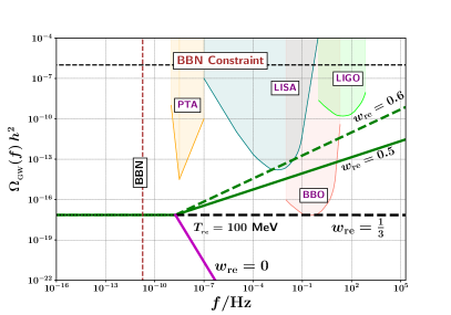
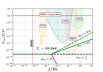
Figure 13: The spectral energy density of relic gravitational waves is shown from the perspective of ongoing and near future GW observatories such as the advanced LIGO, LISA, BBO and PTA. The left panel depicts the spectrum of relic GWs corresponding to reheating EoS $w_{{}_{\rm re}}=0,\leavevmode\nobreak\ 1/3,\leavevmode\nobreak\ 1/2,\leavevmode\nobreak\ 3/5$, plotted in solid purple, dashed black, solid green and dashed green curves respectively, for a fixed reheating temperature $T_{{}_{\rm re}}=100$ MeV and tensor-to-scalar ratio $r\simeq 0.003$. The right panel shows the same but with the higher reheating temperature $T_{{}_{\rm re}}=100$ GeV. The figure demonstrates that primordial GWs with a blue-tilted spectral energy density, $n_{{}_{\rm GW}}>0$, corresponding to relatively stiff EoS during reheating, will be easier to detect in the near future.

Primordial GWs from inflation have not been observed so far, and we currently have an upper bound on the tensor-to-scalar ratio from CMB observations as $r\leq 0.036$. However, Eqs. (186) and (187) indicate that the amplitude of the GW spectral density depends on the tensor-to-scalar ratio $r$, while their tilt at high frequency scales depends upon the reheating EoS $w_{{}_{\rm re}}$. The predicted spectral energy density of GWs has been illustrated in Fig. 13 in the light of both ongoing and near future GW observatories, such as the aLIGO [134], LISA [135], BBO [136] and PTA [137, 138, 139, 140]. The left panel shows the spectrum of relic GWs corresponding to reheating EoS $w_{{}_{\rm re}}=0,\,1/3,\,1/2,\,3/5$, plotted in solid purple, dashed black, solid green and dashed green curves respectively, for a fixed (and quite low) reheating temperature $T_{{}_{\rm re}}=100$ MeV and tensor-to-scalar ratio $r\simeq 0.003$. The right panel depicts the same but with a higher reheating temperature $T_{{}_{\rm re}}=100$ GeV. From Fig. 13, it is clear that primordial GWs with a blue-tilted spectral energy density, $n_{{}_{\rm GW}}>0$, corresponding to relatively stiff EoS during reheating, will be easier to detect in the near future [133].

7 Observational constraints on single field inflation

7.1 Implications of observational constraints

The latest CMB observations by the Planck mission and BICEP/Keck collaboration in Refs. [144, 2] have imposed stringent constraints on the scalar spectral index $n_{{}_{S}}$ and tensor-to-scalar-ratio $r$ at large angular scales, given by

$$\boxed{\leavevmode\nobreak\ n_{{}_{S}}\,\in\,\left[\,0.957,\,0.976\,\right]\,,\quad r(k_{*})\,\leq\,0.036\leavevmode\nobreak\ }\leavevmode\nobreak\ \leavevmode\nobreak\ \mbox{at}\leavevmode\nobreak\ \leavevmode\nobreak\ 95\%\leavevmode\nobreak\ \mbox{C.L}\,.$$ (195)

Additionally, the CMB observations are consistent with $n_{{}_{S}}$ being a constant, without exhibiting any scale dependence or running. The amplitude of scalar fluctuations at the CMB pivot scale has been measured to be [2]

$${\cal P}_{\zeta}(k_{*})\equiv A_{S}=2.1\times 10^{-9}\,,$$ (196)

The constraint $r\leq 0.036$ gets translated to a constraint on the amplitude of the tensor modes

$${\cal P}_{T}(k_{*})\equiv A_{T}\leq 7.56\times 10^{-11}\,,$$ (197)

and hence, using Eq. (162), the Hubble parameter during (slow-roll) inflation is constrained to be

$$\boxed{\leavevmode\nobreak\ H_{\rm inf}\leq 1.93\times 10^{-5}\,m_{p}=4.69\times 10^{13}\ \rm{GeV}\leavevmode\nobreak\ }\,.$$ (198)

We can find the energy scale during inflation using the above parameters and the Friedmann equation $H^{2}_{\rm inf}\simeq\rho_{\rm inf}/{3m_{p}^{2}}$,

$$E_{\rm inf}=(\rho_{\rm inf})^{1/4}\implies E_{\rm inf}\leq 1.4\times 10^{16}\ \rm{GeV}\,,$$ (199)

implying that we are working with scales below the Planck scale ($\sim 10^{18}{\rm GeV}$) which is consistent with our description of inflation using General Relativity. During slow-roll inflation, using Eq. (165), constraints can be placed on $\epsilon_{H}$, $n_{{}_{T}}$ and $\eta_{H}$, namely $\epsilon_{H}\leq 0.00225$, $|n_{{}_{T}}|\leq 0.0045$, and $|\eta_{H}|\simeq 0.02$, respectively. These constraints further imply $w_{\phi}\leq-0.9985$, which is consistent with a state of exponential expansion. For further details on the implications of the latest observations for the inflationary paradigm, see Ref. [152].

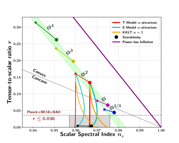
Figure 14: This figure plots the tensor-to-scalar ratio $r$ versus the scalar spectral index $n_{{}_{S}}$ for a number of inflationary potentials (the thinner and thicker dots and curves correspond to $N_{*}=50,\leavevmode\nobreak\ 60$ respectively). These include predictions of plateau potentials such as the Starobinsky model, the Standard Model Higgs inflation, the T-model and E-model $\alpha$-attractors as well as KKLT inflation. The CMB 2$\sigma$ bound $0.957\leq n_{{}_{S}}\leq 0.976$ and the upper bound on the tensor-to-scalar ratio $r\leq 0.036$ are indicated by the shaded grey coloured region. Given the upper bound on $r$, it is easy to see that observations appear to favour concave potentials over the convex ones.

The number of e-folds elapsed between the time when the pivot scale left the Hubble radius until the end of inflation is given by,

$$N_{*}=\frac{1}{m_{p}}\int^{\phi_{*}}_{\phi_{e}}\frac{d\phi}{\sqrt{2\epsilon_{H}}},$$ (200)

where $\phi_{*}$ and $\phi_{e}$ are the field values when the pivot scale exits the horizon and at the end of inflation respectively. Since $\epsilon_{H}$ is almost constant during inflation, the above Eq. (200) can be approximated as,

$$N_{*}\simeq\frac{\Delta\phi}{m_{p}}\times\frac{1}{\sqrt{2\epsilon_{H}}}\leavevmode\nobreak\ ,$$ (201)

with $\Delta\phi=\phi_{*}-\phi_{e}$. Using the expression for the tensor-to-scalar ratio from Eq. (165), we can write the field displacement as

$$\boxed{\leavevmode\nobreak\ \frac{\Delta\phi}{m_{p}}\,\simeq\,2.12\,\left(\frac{N_{*}}{60}\right)\left(\frac{r}{0.01}\right)^{1/2}\leavevmode\nobreak\ }\,,$$ (202)

which is known as the Lyth bound. The above expression implies that in order to generate large, potentially observable, tensor fluctuations, the field displacement during single field inflation must be super-Planckian, namely $\Delta\phi=\phi_{*}-\phi_{e}>m_{p}$, which has important implications for inflationary model building [9, 154]. Models of inflation in which the field displacement is super-Planckian are called large-field models. From an effective field theory (EFT) perspective, such a super-Planckian field displacement in the large-field models imply that an infinite number of terms of the form $a_{n}\,\left(\phi/\Lambda_{c}\right)^{n}\,V(\phi)$ contribute to the inflationary action (82) with each term contributing almost equally, namely $a_{n}\sim\mathcal{O}(1)$ for all $n$ (the cut-off scale $\Lambda_{c}\leq m_{p}$). Hence, the large-field models, although interesting from the observational perspective, are relatively difficult to construct in the EFT, and require additional symmetry constraints from the fundamental UV physics [154].

Note that the BICEP/Keck collaboration have actually constrained the tensor-to-scalar ratio $r$ at the scale $k=0.002\leavevmode\nobreak\ {\rm Mpc}^{-1}$. The tensor-to-scalar ratio $r$ at any $k\in[0.0005,\,0.5]$ can be approximated as,

$$r(k)=\frac{{\cal P}_{T}(k)}{{\cal P}_{S}(k)}=\frac{{\cal P}_{T}(k_{*})}{{\cal P}_{S}(k_{*})}\left[\frac{\left(k/k_{*}\right)^{n_{{}_{T}}}}{\left(k/k_{*}\right)^{n_{{}_{S}}-1}}\right]=\frac{A_{T}}{A_{S}}\left(\frac{k}{k_{*}}\right)^{1-n_{{}_{S}}+n_{{}_{T}}}\,,$$ (203)

showcasing the near scale-invariance of the ratio. Knowing the fact that the spectral index $|n_{{}_{T}}|\ll 1$, we obtain

$$r\big{|}_{k=0.002\leavevmode\nobreak\ {\rm Mpc}^{-1}}\simeq r\big{|}_{k=0.05\leavevmode\nobreak\ {\rm Mpc}^{-1}}\,\left(\frac{0.002}{0.05}\right)^{0.035}\simeq 0.89\times r\big{|}_{k=0.05\leavevmode\nobreak\ {\rm Mpc}^{-1}}\,.$$

Hence, the constraint on $r$ at $k=0.002\leavevmode\nobreak\ {\rm Mpc}^{-1}$ by the BICEP/Keck collaboration can be directly translated into the constraint at the Planck pivot scale $k_{*}=0.05\leavevmode\nobreak\ {\rm Mpc}^{-1}$ within $10\%$ accuracy.

As discussed in Sec. 5, the aforementioned CMB observations [2] by the Planck collaboration span a range of comoving frequency scales $k\in[0.0005,\,0.5]\leavevmode\nobreak\ {\rm Mpc}^{-1}$. Assuming the scalar power spectrum to be strictly of the power-law form given in Eq. (124) with spectral index $n_{{}_{S}}-1$, we can express the variance of $\zeta$ using Eq. (92) as

$$\sigma_{\zeta}^{2}\,\big{|}_{\rm CMB}=A_{S}\,\int_{y_{\rm min}}^{y_{\rm max}}\,\frac{{\rm d}\,y}{y}\,y^{n_{S}-1}\,,$$ (204)

where $y=k/k_{*}$ and $k_{*}=0.05\leavevmode\nobreak\ {\rm Mpc}^{-1}$. Since $k_{\rm min}=0.0005\leavevmode\nobreak\ {\rm Mpc}^{-1}$ and $k_{\rm max}=0.5\leavevmode\nobreak\ {\rm Mpc}^{-1}$, we find $y_{\rm min}=0.1$ and $y_{\rm max}=10$. Assuming the spectral index $n_{{}_{S}}$ to be almost constant, as suggested by the CMB observations, and using the value of $A_{S}$ from Eq. (196), we obtain the variance of CMB fluctuations to be

$$\sigma_{\zeta}^{2}\,\big{|}_{\rm CMB}\simeq 9.7\times 10^{-9}\,,$$ (205)

and the corresponding standard deviation becomes $\sigma_{\zeta}\simeq 9.9\times 10^{-5}$. Hence, the typical size of curvature fluctuations in the CMB sky is often quoted as $\Delta\zeta\simeq 10^{-4}$.

7.2 Dynamics of popular inflationary models

In this section, we discuss how to compute the inflationary observables $\{n_{{}_{S}},\,r\}$ for a given model which supports slow-roll inflation. Traditionally, convex potentials which are steeper than $V(\phi)\propto\phi$ received more attention because they exhibit large field displacement during inflation and generate large (and easier to observe) tensor-to-scalar ratios. Amongst these large field models, the most popular ones were the quadratic potential $V(\phi)\propto\phi^{2}$ and the quartic potential $V(\phi)\propto\phi^{4}$ proposed in Ref. [7] in the context of chaotic inflation. Therefore most lecture notes on inflation provide a detailed discussion on these two chaotic inflationary potentials.

However, the BICEP/Keck bound on the tensor-to-scalar ratio strongly favours concave potentials, including asymptotically flat potentials, which are shallower than $V(\phi)\propto\phi$ (see Fig. 14). Hence we will primarily focus on computing the inflationary observables of a number of asymptotically flat potentials. An asymptotically flat potential has the general functional form

$$V(\phi)=V_{0}\,{\cal F}\left(\lambda\frac{\phi}{m_{p}}\right)\leavevmode\nobreak\ ,$$ (206)

such that ${\cal F}(\phi)\longrightarrow 1$ at large field values $\lambda\phi\gg m_{p}$, where $\lambda$ is a free parameter. Such a potential, schematically represented in Fig. 8, usually features one or two plateau-like wings for large field values away from the minimum of the potential, depending on whether the potential is asymmetric or symmetric. Additionally, an asymptotically flat potential might approach the plateau either exponentially or algebraically. Below we briefly discuss a number of important plateau potentials in light of the latest CMB observations, keeping one example of plateau models belonging to one of the following categories.

1. Symmetric or asymmetric plateau potentials.

2. Single or double parameter plateau potentials.

3. Potentials with an exponential or algebraic approach to the plateau.

Before diving into asymptotically flat potentials, we first discuss monomial potentials which have the simplest functional form. We also use the monomial potential to explicitly demonstrate how to carry out the computation of inflationary observables for a given potential.

7.2.1 Monomial potentials

Monomial potentials are described by the functional form

$$V(\phi)=V_{0}\left(\frac{\phi}{m_{p}}\right)^{p}\,,\quad{\rm with}\quad p>0\,,$$ (207)

for which the potential slow-roll parameters, given in Eqs. (79) and (80), take the form

$$\epsilon_{{}_{V}}(\phi)=\frac{p^{2}}{2}\,\left(\frac{m_{p}}{\phi}\right)^{2}\,;\quad\eta_{{}_{V}}(\phi)=p(p-1)\,\left(\frac{m_{p}}{\phi}\right)^{2}\,.$$ (208)

Under the slow-roll approximations, the value of the inflaton field at the end of inflation, $\phi_{e}$, is given by

$$\epsilon_{{}_{V}}(\phi_{e})=1\,,$$

which, using Eq. (208) leads to

$$\frac{\phi_{e}}{m_{p}}=\frac{p}{\sqrt{2}}\,.$$ (209)

We would next like to compute the value of the inflaton field $\phi_{*}$ during the Hubble-exit of the CMB pivot scale $k_{*}$ for a given potential. Incorporating Eq. (208) into Eq. (81), and using Eq. (209), we obtain

$$N_{*}=\frac{1}{p}\,\int_{\phi_{e}}^{\phi_{*}}\,\frac{\phi\,{\rm d}\phi}{m_{p}^{2}}=\frac{1}{2p}\left[\left(\frac{\phi_{*}}{m_{p}}\right)^{2}-\frac{p^{2}}{2}\right]\,$$

leading to

$$\frac{\phi_{*}}{m_{p}}=\left(2\,p\,N_{*}+\frac{p^{2}}{2}\right)^{1/2}\,,$$ (210)

which yields

$$\epsilon_{{}_{V}}(\phi_{*})=\frac{p}{4\,N_{*}+p}\,;\quad\eta_{{}_{V}}(\phi_{*})=\frac{2\,(p-1)}{4\,N_{*}+p}\,.$$ (211)

In the slow-roll limit, $\epsilon_{H}\simeq\epsilon_{{}_{V}}$ and $\eta_{H}\simeq\eta_{{}_{V}}-\epsilon_{{}_{V}}$. Hence the expressions for the scalar spectral index from Eq. (128) and tensor-to-scalar ratio from Eq. (165) become

$$n_{{}_{S}}-1=2\,\eta_{{}_{V}}(\phi_{*})-6\,\epsilon_{{}_{V}}(\phi_{*})\,;\quad r=16\,\epsilon_{{}_{V}}(\phi_{*})\,,$$ (212)

which for the monomial potential, using Eq. (211), become

$$n_{{}_{S}} = \frac{4\,N_{*}-3\,p}{4\,N_{*}+p}\,;$$ (213)

$$r = \frac{16\,p}{\left(4\,N_{*}+p\right)}\,.$$ (214)

The convex-concave divide can be determined by looking at the $\{n_{{}_{S}},\,r\}$ predictions of the linear potential $V(\phi)\propto\phi$. For $p=1$ in Eq. (207), using Eqs. (213) and (214) we obtain

$$n_{{}_{S}}=\frac{4\,N_{*}-3}{4\,N_{*}+1}\,;\quad r=\frac{16}{4\,N_{*}+1}\,,$$

yielding

$$r=4\left(1-n_{{}_{S}}\right)\,,$$ (215)

which is the dashed grey line, marked as a divider between the predictions of convex and concave potentials in Fig. 14. In order to determine the value of $V_{0}$ (for different $p$), we compute the scalar power spectrum from Eq. (123) under the slow-roll approximations in Eqs. (74) and (75). The slow-roll power spectrum at the pivot scale takes the form

$${\cal P}_{\zeta}(\phi_{*})=\frac{1}{24\pi^{2}}\,\left[\frac{V(\phi_{*})}{m_{p}^{4}}\right]\,\frac{1}{\epsilon_{{}_{V}}(\phi_{*})}\,.$$ (216)

Using Eqs. (210) and (211) and imposing the CMB normalization, we obtain

$$\frac{1}{24\pi^{2}}\,\frac{V(\phi_{*})}{m_{p}^{4}}\,\frac{1}{\epsilon_{{}_{V}}(\phi_{*})}=2.1\times 10^{-9}\,,$$

which yields

$$\frac{V_{0}}{m_{p}^{4}}\simeq 2.5\times 10^{-7}\,\left[\frac{p^{2}}{\left(2\,p\,N_{*}+p^{2}/2\right)^{\frac{p}{2}+1}}\right]\,,$$ (217)

where we typically expect $N_{*}\in[50,\,60]$ depending upon the reheating history, as discussed in App. B. For a given value of $p$, the monomial potential in Eq. (207) contains only a single parameter $V_{0}$, which is completely fixed by the CMB normalisation to be Eq. (217). The predictions for the CMB observables $\{n_{{}_{S}},\,r\}$ of the monomial potential have been shown by the lime coloured shaded region, corresponding to different values of $p$, in Fig. 14. Unfortunately, the latest CMB observations [2, 144] strongly disfavour the entire family of monomial potentials. Hence, we move on to discuss a number of asymptotically flat potentials next that are favoured by the latest observations.

7.2.2 Asymptotically flat potentials

For most functional forms ${\cal F}(\phi)$ of the potential in Eq. (206), it is difficult to analytically integrate Eq. (81) and invert it to determine $\phi_{*}$. For potentials that approach the plateau exponentially, the inversion of Eq. (81) often involves the Lambert function [131, 17]. Therefore one either makes reasonable analytical approximations or computes $\phi_{*}$ numerically [156]. In the following, we will not expand upon the techniques used to compute $\{n_{{}_{S}},\,r\}$, rather we will simply state the known results. The predictions for $\{n_{{}_{S}},\,r\}$ for different asymptotically flat potentials, as plotted in Fig. 14, were obtained numerically in order to be more accurate.

Starobinsky potential

The potential for Starobinsky inflation [3, 157] takes the form

$$V(\phi)=V_{0}\,\left(1-e^{-\frac{2}{\sqrt{6}}\frac{\phi}{m_{p}}}\right)^{2}\,,$$ (218)

which is shown in Fig. 15.

The left wing of the potential is too steep to support inflation (because on the left wing, $\epsilon_{{}_{V}}(\phi)>1$), while the inflationary right wing is asymptotically flat. This potential features a single parameter $V_{0}$, which is related to the scalaron mass $m$ by $V_{0}=\frac{3}{4}\,m^{2}m_{p}^{2}$ [77], and whose value is completely fixed by the CMB normalization (196). The predictions of $\{n_{{}_{S}},r\}$ for the Starobinsky potential are given by

$$n_{{}_{S}}\simeq 1-\frac{2}{N_{*}}\,,\leavevmode\nobreak\ \leavevmode\nobreak\ r\simeq\frac{12}{N_{*}^{2}}\,,\leavevmode\nobreak\ {\rm for}\leavevmode\nobreak\ N_{*}\gg 1\,;$$ (219)

which are shown by black coloured dots in Fig. 14. As per standard convention, the smaller and larger black dots represent $\{n_{{}_{S}},r\}$ predictions corresponding to $N_{*}=50,\,60$ respectively. It is important to note that the predictions of Starobinsky inflation lie at the centre of the observationally allowed region of $\{n_{{}_{S}},r\}$ (shown in grey in Fig. 14), making it one of the most popular inflationary models at present.

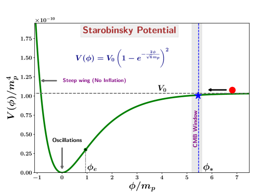
Figure 15: This figure shows the Starobinsky potential given by Eq. (218) with the CMB pivot scale $k_{*}=0.05\leavevmode\nobreak\ {\rm Mpc}^{-1}$ labelled using a blue coloured star, and the grey colour CMB window $k_{\rm CMB}\in\left[0.0005,\,0.5\right]\leavevmode\nobreak\ {\rm Mpc}^{-1}$ in the field space. It is clear that the CMB window constitutes only a tiny portion of the available field space between $\phi_{\rm CMB}$ and the end of inflation $\phi_{e}$.

$\alpha$-attractor potentials

The $\alpha$-attractors belong to a broad class of superconformal inflationary models featuring a parameter $\alpha$ in the inflaton potential, which is inversely proportional to the curvature of the Kahler manifold in supergravity [159, 160]. Two of the most popular models amongst them are the T- and the E-model $\alpha$-attractors, because their predictions for $\{n_{{}_{S}},\,r\}$ are consistent with the latest CMB observations. We begin with the inflationary predictions of the T-model, before moving on to the E-model.

1. T-model $\alpha$-attractor: The T-model $\alpha$-attractor potential [159, 160] is a symmetric plateau potential of the functional form

   $$V(\phi)=V_{0}\,\tanh^{p}{\left(\lambda\frac{\phi}{m_{p}}\right)}\,,$$ (220)

   where $p$ is a positive real number and $\lambda$ is related to $\alpha$ by $\lambda^{2}=\frac{1}{6\alpha}$, see Ref. [152]. For a given value of $p$, the T-model potential has two parameters, namely $V_{0}$ and $\lambda$. As usual, the value of $V_{0}$ is fixed by the CMB normalization while $\lambda$ determines the predicted value of $\{n_{{}_{\rm S}},r\}$ for this potential.

   

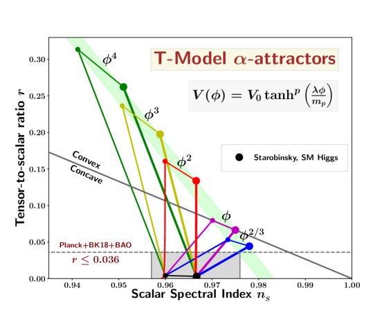
   Figure 16: This figure is a plot of the tensor-to-scalar ratio $r$, versus the scalar spectral index $n_{{}_{\rm S}}$, for the T-model $\alpha$-attractor in Eq. (220) (the thinner and thicker curves correspond to $N_{*}=50,\,60$ respectively). The green, olive, red, magenta and blue curves correspond to $p=4,3,2,1,2/3$, in Eq. (220), respectively. The latest CMB 2$\sigma$ bound $0.957\leq n_{{}_{\rm S}}\leq 0.976$ and the upper bound on the tensor-to-scalar ratio $r\leq 0.036$ are indicated by the grey coloured shaded region. It is important to note that upon increasing the value of $\lambda$, the predictions of the T-model potential for different values of $p$ converge towards the cosmological attractor at the centre, described by Eq. (221). For $\lambda\gtrsim 0.1$, the predictions of the T-model become compatible with the latest CMB $2\sigma$ bound.

   Predictions of the simplest T-model potential, which corresponds to $p=2$ in Eq. (220), are shown by the red coloured curves in Fig. 14. As we vary value of $\lambda$ from $\lambda:0\longrightarrow\infty$, the $r$ versus $n_{{}_{\rm S}}$ values trace out continuous curves in Fig. 14 (the thinner and thicker red curves correspond to $N_{*}=50,\,60$ respectively). We notice that in one limit, namely $\lambda\ll 1$, the CMB predictions for $\{n_{{}_{\rm S}},r\}$ of the T-model match with that of the quadratic potential $V(\phi)\propto\phi^{2}$, owing to the fact that the potential in Eq. (220) for $p=2$ behaves like $V(\phi)\propto\phi^{2}$ for $\lambda\phi\ll m_{p}$. In fact this is true in general for the T-model potential with any value of $p$ in (220), leading to the behaviour $V(\phi)\propto\phi^{p}$ for $\lambda\phi\ll m_{p}$, which is demonstrated in Fig. 16. However in the opposite limit, namely $\lambda\geq 1$ (which results in $\exp\left(\lambda\phi_{*}/m_{p}\right)\gg 1$), the predictions of the T-model become [160]

   $$n_{{}_{\rm S}}\simeq 1-\frac{2}{N_{*}}\,;\quad r\simeq\frac{2}{\lambda^{2}N_{*}^{2}}\,,\leavevmode\nobreak\ {\rm for}\leavevmode\nobreak\ N_{*}\gg 1\,,$$ (221)

   which is independent of $p$ (see Ref. [145]). Due to this property these models are called ‘cosmological attractors’ [160].

2. E-model $\alpha$-attractor:

   The E-model $\alpha$-attractor potential [159, 160] is an asymmetric plateau potential of the functional form

   $$V(\phi)=V_{0}\,\left(1-e^{-\lambda\frac{\phi}{m_{p}}}\right)^{p}\,,$$ (222)

   where $p$ is a positive real number. For $p=2$ and $\lambda=2/\sqrt{6}$, the E-model potential coincides with the Starobinsky potential. In the limit $\lambda\geq 1$ (which results in $\exp\left(\lambda\phi_{*}/m_{p}\right)\gg 1$), the predictions of the E-model become [160]

   $$n_{{}_{\rm S}}\simeq 1-\frac{2}{N_{*}}\,,\leavevmode\nobreak\ \leavevmode\nobreak\ r\simeq\frac{8}{\lambda^{2}N_{*}^{2}}\,,\leavevmode\nobreak\ {\rm for}\leavevmode\nobreak\ N_{*}\gg 1\,,$$ (223)

   which again is independent of $p$ (see [145]). The CMB predictions $\{n_{{}_{\rm S}},r\}$ of the E-model potential are shown by the cyan colour curves in Fig. 14 for the case $p=2$. (the thinner and thicker cyan curves correspond to $N_{*}=50,\,60$ respectively).

In all three of the aforementioned models, the potentials approach the plateau, $V(\phi)\to V_{0}$, exponentially as $\phi\to\infty$. In the following we briefly discuss the strongly motivated D-brane KKLT potential which instead approaches the plateau algebraically.

D-brane KKLT potential

The D-brane KKLT inflation [161, 162, 160] potential (which is analogous to the polynomial $\alpha$-attractor potential [163]) has the following general form

$$V(\phi)=V_{0}\,\left[\frac{\phi^{n}}{\phi^{n}+M^{n}}\right]\,,$$ (224)

where $n$ is a positive integer and $M$ is a fundamental scale of the theory. This is a symmetric plateau potential which approaches the plateau behaviour algebraically, in contrast to the exponential approach to plateau behaviour exhibited by the T-model potential.

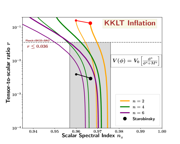
Figure 17: This figure is a plot of the tensor-to-scalar ratio $r$ versus the scalar spectral index $n_{{}_{S}}$ for KKLT inflation (the thinner and thicker curves correspond to $N_{*}=50,\,60$ respectively). The latest CMB 2$\sigma$ bounds on the scalar spectral index $0.957\leq n_{{}_{S}}\leq 0.976$ and the upper bound on the tensor-to-scalar ratio $r\leq 0.036$ are indicated by the grey coloured shaded region. Upon decreasing the value of parameter $M$ in the KKLT potential, the tensor-to-scalar ratio $r$ decreases and hence the model satisfies the CMB bound for smaller values of $M$.

In the limit $M\gg m_{p}$, the CMB window (around the field value $\phi=\phi_{*}$ corresponding to the Hubble-exit of the pivot scale $k_{*}$) belongs to the segment of the potential where it has a monomial power law form $V(\phi)\propto\phi^{n}$, and hence its predictions are strongly disfavoured by observations. In the opposite limit, namely $M\ll m_{p}$, the CMB window belongs to the plateau-like segment, $V(\phi)\simeq V_{0}$, whose predictions satisfy the CMB data very well. Figure 17 shows the $r$ versus $n_{{}_{S}}$ plot for the KKLT potential in Eq. (224) for three different values of $n$ (the thinner and thicker curves correspond to $N_{*}=50,\,60$ respectively). From this figure, it is easy to infer that the predictions of the KKLT potential (224) for $\{n_{{}_{S}},r\}$ do not reach a common attractor regime for different values of $n$ (in contrast to those of the T-model and E-model), rather they cover a large horizontal portion of the observationally allowed region of $n_{{}_{S}}$, as highlighted in Ref. [160]. The relevance of plotting $r$ on a logarithmic scale was highlighted in Ref. [164].

A large class of asymptotically flat potentials can be categorized into different universality classes, depending on their predictions of $\{n_{{}_{S}},\,r\}$. In this scheme, the T- and E-model $\alpha$-attractors belong to the same universality class, while the D-brane KKLT inflation belongs to a different class. We will not elaborate further on this point and direct the interested readers to Refs. [165, 166, 167, 168, 169, 170].

The number of single field inflationary models proposed in the literature is rather large at present, out of which we have chosen only a few to illustrate their inflationary dynamics in these lecture notes. For a more extensive list of inflationary models, see Ref. [17]. Furthermore, we have discussed the aforementioned models from a phenomenological point of view, without much reference to their microscopic/fundamental origin. Inflationary model building from fundamental physics, such as String Theory, is an important and active area of research, see Ref. [9, 154].

8 Post-inflationary inflaton dynamics and reheating

The universe makes a transition from the accelerated expansion during inflation to a decelerated expansion at the end of inflation when $\epsilon_{H}=1\,\Rightarrow\,\dot{\phi}^{2}=V(\phi)$. After the end of inflation, the inflaton field oscillates around the minimum of the potential. The time-averaged Hubble parameter of this decelerating universe keeps falling as $\langle H\rangle\propto 1/t$ on time scales longer than the period oscillation, and hence at sufficiently late times, we can ignore the expansion of space while dealing with the inflaton oscillations [171]. Such oscillations are called coherent oscillations. We will begin with a discussion on the coherently oscillating inflaton field after inflation, in the absence of any external coupling. Then we will move on to study the decay of the inflaton in the presence of an external coupling.

8.1 Coherently oscillating scalar field

During coherent oscillations of a scalar field, since the expansion of the universe can be ignored on shorter time scales, the density of the field

$$\rho_{\phi}\equiv\frac{1}{2}\dot{\phi}^{2}+V(\phi)\simeq V(\phi_{0})\,,$$ (225)

is almost a constant over oscillation time scales. Here $\phi_{0}(t)$ is the amplitude of the oscillations which decreases slowly due to the expansion of the universe on time scales that are much longer than the time period of oscillations of the inflaton field. Such an approximation is usually known as the adiabatic approximation. Using Eq. (225) the inflaton speed can be expressed as

$$\dot{\phi}=\sqrt{2\,\big{(}V(\phi_{0})-V(\phi)\big{)}}\,.$$ (226)

Let us calculate the time averaged equation of state $\langle w_{\phi}\rangle$ and time period of coherent oscillations of the inflaton around a monomial potential

$$V(\phi)=V_{0}\left(\frac{\phi}{m_{p}}\right)^{2n}\,;\quad{\rm with}\quad n>0\,.$$ (227)

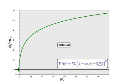
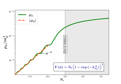
Figure 18: Evolution of the inflaton field dynamics (left panel) and energy density (right panel) is shown as a function of the number of e-folds before the end of inflation, $N_{e}$. After the end of inflation, the inflaton $\phi$ begins to oscillate around the minimum of the potential. At late times, the oscillations becomes coherent and the time-averaged equation of state becomes $\langle w_{\phi}\rangle=0$, leading to a pressureless matter-like behaviour. Consequently, the time averaged energy density of the inflaton falls as $\rho_{\phi}\propto 1/a^{3}$.

8.1.1 Time-averaged equation of state

The equation of state of a scalar field is defined as

$$w_{\phi}=\frac{p_{\phi}}{\rho_{\phi}}=\frac{\frac{1}{2}\,\dot{\phi}^{2}-V(\phi)}{\frac{1}{2}\,\dot{\phi}^{2}+V(\phi)}\,,$$ (228)

from which we get

$$\Rightarrow 1+w_{\phi}=\frac{\dot{\phi}^{2}}{\rho_{\phi}}=2\,\frac{V(\phi_{0})-V(\phi)}{V(\phi_{0})}\,,$$

leading to

$$1+w_{\phi}=2\,\left[1-\frac{V(\phi)}{V(\phi_{0})}\right]\,.$$ (229)

For the monomial potential in Eq. (227), the above expression becomes

$$1+w_{\phi}=2\,\left[1-\left(\frac{\phi}{\phi_{0}}\right)^{2n}\right]\,.$$ (230)

Averaging the above quantity over a period of an oscillation ($T_{\rm osc}$) gives us

$$\langle 1+w_{\phi}\rangle\equiv 1+\langle w_{\phi}\rangle=\frac{\int_{0}^{T_{\rm osc}}\,{\rm d}t\,\left(1+w_{\phi}\right)}{\int_{0}^{T_{\rm osc}}\,{\rm d}t}=\frac{2\,\int_{-\phi_{0}}^{\phi_{0}}\,{\rm d}\phi\,\left(\frac{1+w_{\phi}}{\dot{\phi}}\right)}{2\int_{-\phi_{0}}^{\phi_{0}}\,{\rm d}\phi\,\left(\frac{1}{\dot{\phi}}\right)}\,.$$

Incorporating

$$\dot{\phi}=\sqrt{2\,V(\phi_{0})\left(1-\frac{V(\phi)}{V(\phi_{0})}\right)}=\sqrt{2\,V(\phi_{0})\left(1-\left(\frac{\phi}{\phi_{0}}\right)^{2n}\right)}\,,$$

and using Eq. (230), we get

$$1+\langle w_{\phi}\rangle=\frac{2\,\int_{-\phi_{0}}^{\phi_{0}}\,{\rm d}\phi\,\frac{1-\left(\phi/\phi_{0}\right)^{2n}}{\sqrt{2\,V(\phi_{0})\left(1-\left(\phi/\phi_{0}\right)^{2n}\right)}}}{\int_{-\phi_{0}}^{\phi_{0}}\,{\rm d}\phi\,\frac{1}{\sqrt{2\,V(\phi_{0})\left(1-\left(\phi/\phi_{0}\right)^{2n}\right)}}}\,.$$

Defining $y=\phi/\phi_{0}$ so that $\phi\to\phi_{0}\,\implies\,y\to 1$, we get

$$1+\langle w_{\phi}\rangle=\frac{2\,\int_{-1}^{1}\,{\rm d}y\,\frac{1-y^{2n}}{\sqrt{1-y^{2n}}}}{\int_{-1}^{1}\,{\rm d}y\,\frac{1}{\sqrt{1-y^{2n}}}}$$

which can be written as

$$1+\langle w_{\phi}\rangle=\frac{2\,\int_{0}^{1}\,{\rm d}y\,\left(1-y^{2n}\right)^{1/2}}{\int_{0}^{1}\,{\rm d}y\,\left(1-y^{2n}\right)^{-1/2}}\,.$$ (231)

Using the integral relations

$$\int_{0}^{1}\,{\rm d}y\,\left(1-y^{2n}\right)^{1/2}=\frac{\Gamma\left(\frac{1}{2}\right)\Gamma\left(1+\frac{1}{2n}\right)}{2\,\Gamma\left(\frac{3}{2}+\frac{1}{2n}\right)}\,;\quad\int_{0}^{1}\,{\rm d}y\,\left(1-y^{2n}\right)^{-1/2}=\frac{\Gamma\left(\frac{1}{2}\right)\Gamma\left(1+\frac{1}{2n}\right)}{\Gamma\left(\frac{1}{2}+\frac{1}{2n}\right)}\,,$$ (232)

we get

$$1+\langle w_{\phi}\rangle=\frac{\Gamma\left(\frac{1}{2}+\frac{1}{2n}\right)}{\Gamma\left(\frac{3}{2}+\frac{1}{2n}\right)}=\frac{2n}{n+1}\,,$$

leading to the well-known final expression for the time-averaged equation of state, as first obtained in Ref. [171], to be

$$\boxed{\leavevmode\nobreak\ \langle w_{\phi}\rangle=\frac{n-1}{n+1}\leavevmode\nobreak\ }\,.$$ (233)

Hence, for oscillations around a quadratic potential ($n=1$), $\langle w_{\phi}\rangle=0$ (matter-like) and around a quartic potential ($n=2$), $\langle w_{\phi}\rangle=1/3$ (radiation-like), while $\langle w_{\phi}\rangle\leq-1/3$ for $n\leq 1/2$, which leads to an accelerated expansion.

8.1.2 Period of an anharmonic oscillator

The time period of oscillations is defined as

$$T_{\rm osc}=\int_{0}^{T_{\rm osc}}{\rm d}t=2\,\int^{\phi_{0}}_{-\phi_{0}}\frac{{\rm d}\phi}{\dot{\phi}},$$ (234)

which can be written for the monomial potential (227), using Eq. (226), as

$$T_{\rm osc}=\frac{2}{\sqrt{2V(\phi_{0})}}\int_{-\phi_{0}}^{\phi_{0}}\,{\rm d}\phi\frac{1}{\left[1-\left(\phi/\phi_{0}\right)^{2n}\right]^{1/2}}\,.$$

Using the variable redefinition $y=\phi/\phi_{0}$, we obtain

$$T_{\rm osc}=\frac{2\phi_{0}}{\sqrt{2V(\phi_{0})}}\int_{-1}^{1}\,{\rm d}y\frac{1}{\left[1-y^{2n}\right]^{1/2}}=\frac{4\phi_{0}}{\sqrt{2V(\phi_{0})}}\int_{0}^{1}\,{\rm d}y\left[1-y^{2n}\right]^{-1/2}$$

Now using the integral identity in Eq. (232), we obtain

$$T_{\rm osc}=2\sqrt{2\pi}\,\frac{\phi_{0}}{\sqrt{V(\phi_{0})}}\frac{\Gamma\left(1+\frac{1}{2n}\right)}{\Gamma\left(\frac{1}{2}+\frac{1}{2n}\right)}\,,$$

which, using Eq. (227), yields the final expression

$$\boxed{\leavevmode\nobreak\ T_{\rm osc}=2\sqrt{2\pi}\,\frac{m_{p}}{\sqrt{V_{0}}}\,\frac{\Gamma\left(1+\frac{1}{2n}\right)}{\Gamma\left(\frac{1}{2}+\frac{1}{2n}\right)\leavevmode\nobreak\ }\,\left(\frac{\phi_{0}}{m_{p}}\right)^{1-n}}\,.$$ (235)

Eq. (235) clearly demonstrates that for $n=1$, the period of oscillation is independent of the amplitude $\phi_{0}$. Note that in deriving Eqs. (233) and (235), we never used the assumption that $n$ is an integer in Eq. (207). Hence our primary results given in Eqs. (233) and (235) are valid for all $n\in\mathbb{R}^{+}$. Also notice that for $n>1$, the period of oscillation becomes shorter as we increase the amplitude of the oscillations $\phi_{0}$, while for $n<1$, the period becomes longer with higher values of $\phi_{0}$. It means that the quadratic potential is a special case (simple harmonic oscillator) for which the frequency of oscillations is completely independent of the amplitude, as we learned a long way back in our introductory physics course [172], thanks to the great Galileo Galilei who first made this crucial observation.

Before moving on to discuss the decay of the inflaton, let us stress that Eqs. (233) and (235) are also (more or less) applicable to asymptotically flat potentials because the coherent oscillations after the end of inflation are only sensitive to the functional form of the minimum of the potential, rather than to the inflationary plateau wing. However, if the plateau is flat enough, then during the first few oscillations, the inflaton field explores some parts of the plateau, as a result of which the inflaton field behaves like a self-interacting oscillating condensate. To be precise, consider oscillations around the minimum of a plateau potential of the functional form

$$V(\phi)=V_{0}\left(\frac{\phi}{m_{p}}\right)^{2n}-|U(\phi)|\,,$$ (236)

where the attractive self-interaction term, $U(\phi)$, is due to the flattening of the potential at large field values. The potential is schematically plotted in Fig. 19.

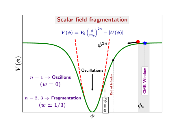
Figure 19: This figure schematically illustrates a typical asymptotically flat inflaton potential of the form (236). Here $\phi_{c}$ is the critical field value around which the potential flattens away from its monomial form $V(\phi)\sim\phi^{2n}$. The attractive self-interaction $U(\phi)$ results in the fragmentation of the oscillating inflaton condensate due to non-linear effects. For $n=1$, these fragments behave as non-relativistic oscillons, while for $n>1$, the fragments behave as transients which quickly decay into scalar radiation.

The inflaton condensate oscillating around the potential (236) fragments to form dense scalar field lumps due to the presence of the non-linear attractive self-interaction $U(\phi)$. For $n=1$, i.e., oscillations around a predominantly quadratic potential (which flattens for large field values), these scalar field lumps behave like quasi-solitonic objects whose localised energy density remains fixed while the field value oscillates with time around a fixed radial profile, as demonstrated in Refs. [173, 174]. Such quasi-breather scalar field lumps/configurations are known as pulsons or oscillons. Oscillons are quite long lived and have interesting cosmological implications. However, in these pedagogical lecture notes, we do not elaborate further on oscillons and direct the interested readers to Refs. [173, 175, 176, 174, 177, 178, 179, 180, 181, 182]. For $n>1$, the fragments behave as transients which quickly decay into scalar radiation with $w\simeq 1/3$ as discussed in Ref. [174].

In the above analysis, we ignored the coupling of the inflaton field to other (scalar, spinor and tensor) degrees of freedom. In the presence of external coupling, the inflaton decays into the particles of the coupled fields which eventually leads to reheating of the universe to the hot Big Bang phase, as we now begin to explore.

8.2 External coupling and decay of the inflaton condensate

Due to its external coupling, the inflaton condensate $\phi$ decays into one or more offspring fields ($\chi,\,\psi,\,A_{\mu}$ etc), which then interact and decay into further particles before finally thermalizing leading to the commencement of Big Bang Nucleosysthesis (BBN). Reheating is supposed to be (directly or indirectly) the origin of (almost) all matter in the hot Big Bang universe [27]. During the post-inflationary oscillations, the inflaton decay can occur either perturbatively, due to the decay of individual massive inflaton particles, or non-perturbatively via the mechanism of parametric resonance due to the coherent nature of the inflaton field oscillations. Which of these two ways is predominant depends upon the amplitude of inflaton oscillations as well as the nature of the coupling between the inflaton and other bosonic/fermionic degrees of freedom.

8.2.1 Perturbative reheating

In the perturbative reheating framework, the inflaton field (after the end of inflation) is assumed to be comprised of a large number of massive inflaton particles (of low momenta), each of which can decay independently into the quanta of the coupled offspring fields, and the corresponding decay rate $\Gamma$ can be computed using the standard Feynman rules [27]. The perturbative theory of reheating was originally developed in the context of the new inflationary scenario in [23]. Phenomenologically, it amounts to adding a friction term $\Gamma{\dot{\phi}}$ to the classical equation of motion of the inflaton field oscillating around the minimum of its potential  [23, 24], i.e.

$${\ddot{\phi}}+\left(3H+\Gamma\right){\dot{\phi}}+V_{,\phi}(\phi)=0\,.$$ (237)

The perturbative theory of reheating works well if either (a) the inflaton decays only into fermions $\psi$ through a Yukawa-type interaction $h\psi{\bar{\psi}}\phi$, with a weak coupling constant $h$ satisfying $h^{2}\ll m_{\phi}/m_{p}$, or (b) the coupling of the inflaton to a scalar boson $\chi$, described by the interaction $\frac{1}{2}g^{2}\phi^{2}\chi^{2}$, is weak with $g\ll 3\times 10^{-4}$, making particle production via non-perturbative effects (parametric resonance) ineffective [27].

In the perturbative regime, since inflaton decay is a slow process, the reheating EoS is given by the time averaged EoS of the inflaton field during its oscillations around the minimum of the potential, i.e $w_{\rm re}=\langle w_{\phi}\rangle$. For monomial potentials, $V(\phi)\propto\phi^{2n}$, the equation of state during reheating is given by Eq. (233) to be

$$w_{\rm re}=\langle w_{\phi}\rangle=\frac{n-1}{n+1}\,.$$

At the beginning of reheating, $H\gg\Gamma$, otherwise significant particle production during inflation will modify the inflaton potential and might spoil the CMB predictions. Hence reheating in the perturbative scenario gets completed only when the (decreasing) expansion rate becomes equal to the decay rate at late times so that $H\simeq\Gamma$. Following thermalization, the reheating temperature can be computed by considering

$$\Gamma\simeq H=\sqrt{\frac{1}{3m_{p}^{2}}\,\rho(T_{\rm re})}\Rightarrow\Gamma=\sqrt{\frac{1}{3m_{p}^{2}}\,\frac{\pi^{2}}{30}\,g_{*}(T_{\rm re})\,T_{\rm re}^{4}}$$

leading to

$$\boxed{\leavevmode\nobreak\ T_{\rm re}\simeq\left(\frac{\pi^{2}\,g_{*}}{90}\right)^{-1/4}\,\Big{(}\Gamma\,m_{\rm p}\Big{)}^{1/2}=2.4\times 10^{18}\times\left(\frac{\pi^{2}\,g_{*}}{90}\right)^{-1/4}\,\Big{(}\frac{\Gamma}{m_{p}}\Big{)}^{1/2}\leavevmode\nobreak\ {\rm GeV}\leavevmode\nobreak\ }\,,$$ (238)

which, intriguingly, is independent of both the duration of inflation and the properties of the inflaton potential $V(\phi)$. As stressed above, since the coupling between the inflaton and the external fields can alter, via radiative corrections, the shape of $V(\phi)$ during inflation, this places strong constraints on the total decay rate [27, 28, 184]. This in turn implies that the reheating temperature in perturbative models will be relatively low, typically $T_{\rm re}<10^{9}$ GeV (see the introductory lecture notes), and hence the duration of reheating $N_{\rm re}$ is quite long and reheating is inefficient in the perturbative regime [27].

8.2.2 Non-perturbative reheating

For inflationary models in which the main source of reheating is through the decay of the inflaton into bosons, non-perturbative effects might become important to the coherent oscillations of the inflaton field. The scenario is analogous to particle production in the presence of time dependent external fields. To be concrete, we will focus on the scenario of the inflaton coupled to a single massless scalar offspring field $\chi$ through an interaction ${\cal I}(\varphi,\chi)$, with the model being described by the action

$$S[g_{\mu\nu},\,\varphi,\,\chi]=\int{\rm d}^{4}x\leavevmode\nobreak\ \sqrt{-g}\,\left[\frac{m_{p}^{2}}{2}\,R-\frac{1}{2}\,\partial_{\mu}\varphi\,\partial_{\nu}\varphi\,g^{\mu\nu}-\frac{1}{2}\,\partial_{\mu}\chi\,\partial_{\nu}\chi\,g^{\mu\nu}-V(\varphi)-{\cal I}(\varphi,\chi)\right]\,.$$ (239)

The corresponding field equations are given by

$$\ddot{\varphi}-\frac{\nabla^{2}}{a^{2}}\varphi+3H\dot{\varphi}+V_{,\varphi}+{\cal I}_{,\varphi}=0\leavevmode\nobreak\ ,$$ (240)

$$\ddot{\chi}-\frac{\nabla^{2}}{a^{2}}\chi+3H\dot{\chi}+{\cal I}_{,\chi}=0\,,$$ (241)

with

$$H^{2}\,=\,\frac{1}{3\,m_{p}^{2}}\,\left[\frac{1}{2}\,\dot{\varphi}^{2}+\frac{1}{2}\,\frac{\vec{\nabla}\varphi}{a}.\frac{\vec{\nabla}\varphi}{a}+V(\varphi)+\frac{1}{2}\,\dot{\chi}^{2}+\frac{1}{2}\,\frac{\vec{\nabla}\chi}{a}.\frac{\vec{\nabla}\chi}{a}+{\cal I}(\varphi,\,\chi)\right]\,.$$ (242)

Eqs. (240)–(242) indicate that the dynamics of reheating is a complicated, non-linear and non-thermal process. Hence, various approximations corresponding to neglecting different terms in the above set of equations are usually carried out in the literature, some of which have been indicated by the arrow marks in the following (to be made more explicit later).

$$\ddot{\varphi}-\cancelto{0}{\frac{\nabla^{2}}{a^{2}}}\varphi+\cancelto{0}{3H\dot{\varphi}}+V_{,\varphi}(\varphi)+\cancelto{0}{{\cal I}_{,\varphi}}=0\,$$

$$\ddot{\chi}-\frac{\nabla^{2}}{a^{2}}\chi+\cancelto{0}{3H\dot{\chi}}+{\cal I}_{,\chi}=0\,,$$

$$H^{2}\,=\,\frac{1}{3\,m_{p}^{2}}\,\left[\frac{1}{2}\,\dot{\varphi}^{2}+\frac{1}{2}\,\cancelto{0}{\frac{\vec{\nabla}\varphi}{a}.\frac{\vec{\nabla}\varphi}{a}}+V(\varphi)+\frac{1}{2}\,\cancelto{0}{\dot{\chi}^{2}}+\frac{1}{2}\,\cancelto{0}{\frac{\vec{\nabla}\chi}{a}.\frac{\vec{\nabla}\chi}{a}}+\cancelto{0}{{\cal I}(\varphi,\,\chi)}\right]\,.$$

One also makes further assumptions by considering a particular form of the potential, for example, previously we considered a monomial potential given in Eq. (227). In these notes, we will focus on a quadratic-quadratic inflaton coupling to the offspring field $\chi$ of the form

$${\cal I}(\varphi,\,\chi)=\frac{1}{2}\,g^{2}\,\varphi^{2}\,\chi^{2}\,.$$ (243)

In the post inflationary epoch, the universe goes through inflaton decay, thermalization and reheating via a sequence of successive stages as discussed below (see Refs. [25, 26, 27, 28, 29, 30, 31]).

(1) Preheating:

The early stage of inflaton decay, known as preheating, involves the phenomenon of parametric resonance brought about by the coherent oscillations of the inflaton $\phi$ around the minimum of its potential [28]. In order to understand this regime, one usually makes a number of (physically reasonable) approximations. Since the inflaton behaves as a homogeneous condensate at the end of inflation, its gradient term in Eq. (240) may be dropped. Furthermore, since we are working in the cold inflationary regime for which particle production can be ignored during inflation, we assume that the $\chi$ field is in its vacuum at the beginning of reheating. The energy budget of the universe in this regime is dominated by the inflaton condensate, hence $\chi$ can be treated as a test field.

A convenient way to characterise the dynamics during the early stages of preheating is to linearize the field fluctuations in Eqs. (240)-(241) and carry out the standard Floquet analysis. To begin with, we split each of the field contents in the Eqs. (240)-(242) into a homogeneous background and small fluctuations around that background, namely

$$\varphi(t,\vec{x}) = \phi(t)+\delta\varphi(t,\vec{x})\,;$$ (244)

$$\chi(t,\vec{x}) = \bar{\chi}(t)+\delta\chi(t,\vec{x})\,.$$ (245)

As discussed before, since the $\chi$ field is expected to be in its vacuum state at the end of inflation, we have $\bar{\chi}(t)\simeq 0$, leading to $\delta\chi(t,\vec{x})=\chi(t,\vec{x})$. From hereon, we will simply denote the fluctuations $\delta\chi$ as $\chi$. We use the following approximations to retain only terms that are linear in the fluctuations $\delta\varphi$ and $\chi$.

1. The energy density of the system is predominantly contained in the homogeneous inflaton condensate $\phi(t)$, i.e.

   $$|\phi(t)|\,\gg\,|\delta\varphi(t,\vec{x})|,\,|\chi(t,\vec{x})|\,;$$

   and

   $$\rho_{\phi}\,\gg\,\rho_{\chi},\,\rho_{\delta\varphi}\,.$$

2. Since $\bar{\chi}(t)=0$, the interaction term ${\cal I}(\varphi,\chi)$ becomes

   $${\cal I}(\varphi,\chi)={\cal I}(\phi+\delta\varphi,\chi)\simeq\frac{1}{2}\,g^{2}\,\phi^{2}(t)\,\chi^{2}\,,$$

   which can be dropped from the Friedmann Eq. (242) at linear order. Furthermore, we find

   $${\cal I}_{,\varphi}\equiv g^{2}\,\varphi\,\chi^{2}=g^{2}\,\left(\phi(t)+\delta\varphi\right)\,\chi^{2}\simeq g^{2}\,\phi(t)\,\chi^{2}\,,$$

   which can be dropped from the evolution Eq. (240) at linear order. Similarly, the last term of the left hand side of Eq. (240) becomes

   $${\cal I}_{,\chi}\equiv g^{2}\,\varphi^{2}\,\chi=g^{2}\,\left(\phi(t)+\delta\varphi\right)^{2}\,\chi\simeq g^{2}\,\phi^{2}(t)\,\chi$$

   at linear order.

3. Under the linear approximation, the inflaton potential becomes

   $$V(\varphi)=V(\phi+\delta\varphi)\simeq V(\phi)+V_{,\phi}(\phi)\,\delta\varphi$$

   and its derivative becomes

   $$V_{,\varphi}(\varphi)=V_{,\varphi}(\phi+\delta\varphi)\simeq V_{,\phi}(\phi)+V_{,\phi\phi}(\phi)\,\delta\varphi\,.$$

We again stress that these approximations are valid during the early stages of preheating, before backreactions from $\delta\varphi$ and $\chi$ become significant, i.e., before $\rho_{\delta\varphi,\chi}\sim\rho_{\phi}$. Under the aforementioned approximations, Eqs. (240)-(241) become

$$\ddot{\phi}+3H\dot{\phi}+V_{,\phi} = 0\,;$$ (246)

$${\delta\ddot{\varphi}}+3H{\delta\dot{\varphi}}+\left[-\frac{\nabla^{2}}{a^{2}}+V_{,\varphi\varphi}(\phi)\right]\delta\varphi = 0\,;$$ (247)

$$\ddot{\chi}+3H\dot{\chi}+\left[-\frac{\nabla^{2}}{a^{2}}+g^{2}\,\phi^{2}\right]\,\chi = 0\,,$$ (248)

and the Friedmann Eq. (242) becomes

$$H^{2}=\frac{1}{3\,m_{p}^{2}}\,\left[\frac{1}{2}\,\dot{\phi}^{2}+V(\phi)\right]\,.$$ (249)

Note that in Eqs. (246) and (249) we have dropped the $\delta\varphi$ terms in order to describe the background dynamics in terms of the purely homogeneous condensate at the end of inflation. Hence, they represent the background equations, w.r.t which fluctuations are defined. The corresponding equations for the evolution of the Fourier modes $\delta\varphi_{k}$ and $\chi_{k}$ take the following form

$$\ddot{\delta\varphi_{k}}+3H\dot{\delta\varphi_{k}}+\left[\frac{k^{2}}{a^{2}}+V_{,\phi\phi}(\phi)\right]\delta\varphi_{k} = 0\,;$$ (250)

$$\ddot{\chi}_{k}+3H\dot{\chi}_{k}+\left[\frac{k^{2}}{a^{2}}+g^{2}\,\phi^{2}\right]\chi_{k} = 0\,.$$ (251)

Eqs. (250) and (251) describe two independent parametric oscillators with time-dependent damping terms $3H\dot{\delta\varphi_{k}}$ and $3H\dot{\chi_{k}}$ and parametric frequencies of the form

$$\Omega^{2}_{\delta\varphi}(k,t)=\frac{k^{2}}{a^{2}}+V_{,\phi\phi}(\phi)\,;\quad\Omega^{2}_{\chi}(k,t)=\frac{k^{2}}{a^{2}}+g^{2}\,\phi^{2}(t)\,.$$

For simplicity, we ignore the expansion of the background space ($H\simeq 0,\,a=1$), which is a reasonable assumption on (the inflaton oscillation) time scales that are much shorter compared to the time scale of expansion of space, $H^{-1}$. Since we will not discuss inflaton fragmentation, we further ignore the inflaton fluctuations $\delta\varphi$. Consequently, the system is reduced to

$$\ddot{\chi}_{k}+\left[k^{2}+g^{2}\,\phi^{2}(t)\right]\chi_{k} = 0\,;$$ (252)

$$\ddot{\phi}\,+\,V_{,\phi}(\phi) = 0\,.$$ (253)

Eq. (252) describes the motion of an oscillator with a time dependent frequency $\Omega_{k}^{2}(t)=k^{2}+g^{2}\phi^{2}(t)$. Since $\phi(t)$ is oscillating, $\Omega_{k}^{2}(t)$ also oscillates with time. Thus, Eq. (252) describes the motion of a parametric oscillator and can lead to exponential growth of $\chi_{k}$ for certain ranges of $k$ due to a phenomenon called parametric resonance. For inflaton oscillations around a quadratic potential

$$V(\phi)=\frac{1}{2}\,m^{2}\,\phi^{2}\,,$$

the solution to Eq. (253) is given by

$$\phi(t)=\phi_{0}\,\cos{\left(mt\right)}\,,$$ (254)

for which Eq. (252) simplifies to

$$\ddot{\chi}_{k}+\left[\left(k^{2}+\frac{g^{2}\phi^{2}_{0}}{2}\right)+\frac{g^{2}\phi^{2}_{0}}{2}\,\cos{(2mt)}\right]\chi_{k}=0\,,$$

which, under the change in variable

$$T=mt+\frac{\pi}{2}\,$$

takes the form of the Mathieu Equation

$$\boxed{\leavevmode\nobreak\ \frac{{\rm d}^{2}\chi_{k}}{{\rm d}T^{2}}+\left[A_{k}-2q\,\cos(2T)\,\right]\chi_{k}=0\leavevmode\nobreak\ }$$ (255)

where the resonance parameters $q,\,A_{k}$ are given by

$$q=\frac{g^{2}}{4}\left(\frac{\phi_{0}}{m}\right)^{2}\,;\quad A_{k}=\left(\frac{k}{m}\right)^{2}+2\,q\,.$$ (256)

In Floquet theory [185, 186, 131], the Mathieu equation admits solutions of the form

$$\chi_{k}(T)=\mathcal{M}_{k}^{(+)}(T)\leavevmode\nobreak\ e^{\mu_{k}T}+\mathcal{M}_{k}^{(-)}(T)\leavevmode\nobreak\ e^{-\mu_{k}T}$$ (257)

where $\mathcal{M}_{k}^{(+)}$ and $\mathcal{M}_{k}^{(-)}$ are periodic functions and $\mu_{k}$ is called the Floquet/Mathieu exponent. For certain ranges of values of $k$ if ${\real(\mu_{k})}\neq 0$, the solution to the Mathieu equation, namely Eq. (257), grows exponentially with time leading to parametric resonance.

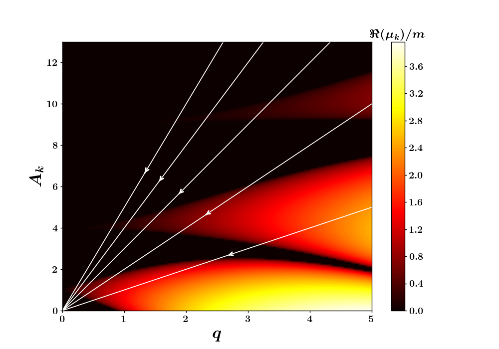
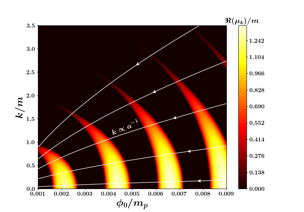
Figure 20: The instability charts of the Mathieu Eq. (255) are shown here. The magnitude of the Floquet exponent $\mu_{k}$ depends upon $A_{k}=(k/m)^{2}+2q$, where $q=g^{2}\phi^{2}_{0}/(4m^{2})$ being the resonance parameter. The parameter space $\{q,\,A_{k}\}$ can be divided into two parts- unstable (yellow) and stable (maroon). Resonant production of $\chi$-particles from the inflaton happens when $A_{k}$ and $q$ lie in the unstable region, corresponding to the Floquet exponent $\real(\mu_{k})\neq 0$. The white lines indicate the redshifting of physical momenta $k_{p}\propto k/a$, and the inflaton amplitude $\phi_{0}(t)$ at longer time scales due to the expansion of the universe. The left panel depicts the instability chart in terms of the Mathieu parameters $\{q,\,A_{k}\}$, while the right panel shows the same in terms of the physical parameters $\{\phi_{0},\,k\}$.

The instability chart of the Mathieu equation is shown in Fig. 20, where the magnitude of ${\real(\mu_{k})}$ is plotted as a function of the parameters $\phi_{0}$ and $k$ (both being positive). The regions in the chart are broadly classified into ‘stable’ where ${\real(\mu_{k})}=0$ and ‘unstable’ where ${\real(\mu_{k})}\neq 0$. The solutions to Eq. (255) in the unstable regions contain an exponential instability $\chi_{k}\propto\exp(\mu_{k}T)$, which corresponds to an exponential growth in the occupation number density $n_{\chi}(k)$ of the produced particles [28], i.e.

$$n_{\chi}(k)\equiv\frac{1}{2\Omega_{\chi}}\left[\bigg{|}\frac{{\rm d}{\chi_{k}}}{{\rm dT}}\bigg{|}^{2}+\Omega_{\chi}^{2}\,|\chi_{k}|^{2}\right]-\frac{1}{2}\,\propto\,e^{2\mu_{k}T}\,,$$

which can be interpreted as explosive particle production.

In accordance with the band structure of these stable and unstable regions, parametric resonance can be further classified into narrow and broad regimes.

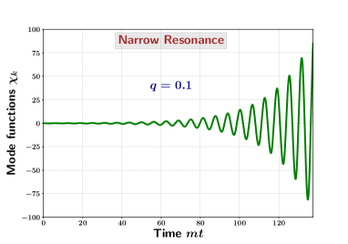
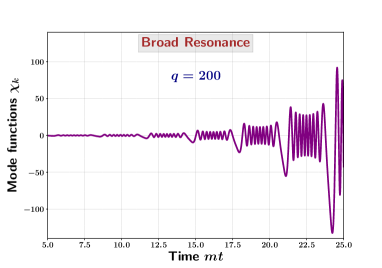
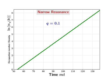
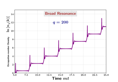
Figure 21: Narrow parametric resonance of the $\chi$-field for $q\sim 0.1$ is shown in green (left) and broad parametric resonance for $q\sim 200$ (right) is shown in purple for modes lying inside the narrow and broad resonance bands, respectively, corresponding to the Mathieu Eq. (255). The upper figures show the growth in the amplitude of the mode functions, while the lower ones show the growth of the (logarithm of the) occupation-number density, $n_{\chi}(k)$. The particle number densities grow exponentially for such resonant modes, with broad resonance being more efficient than the narrow one. Note that in the broad band resonance, peaks in the particle number density occur whenever the inflaton field value vanishes, i.e., $\phi(t)=0$.

1. Narrow Resonance:

   Narrow band resonance occurs when the instability band width is quite narrow. From Fig. 20 for Eq. (255), the narrow resonance is observed for $q\rightarrow 0$ and $A_{k}\rightarrow n^{2}$ ($n\in\mathbb{Z}^{+}$). The width of a narrow band is given by $\Delta k/m\sim q^{n}$. Such resonance occurs only due to the dense occupation of $\chi$ modes leading to a smooth exponential increase of $n_{k}$ as shown in Fig. 21. The first narrow instability band corresponds to $n=1$, which is described by $A_{k}\sim 1\pm q$. It is the widest and most important band in this narrow regime, which can be interpreted as the production of two $\chi$-particles with momentum $k\approx m$ from the decay of two inflaton particles, which is an excellent match with the perturbative analysis. Indeed, narrow resonance bands with higher $n$ can be interpreted as the simultaneous non-perturbative decay of $2n$-inflaton particles into a pair of $\chi$-particles with momentum $k\approx nm\geq m$. In the narrow regime, since the interactions are weak, $\Omega_{\chi}^{2}(k)\approx k^{2}$ stays almost a constant. Hence the inflaton condensate continues to oscillate coherently.

2. Broad Resonance:

   Broad band parametric resonance corresponds to the broader instability regions in Fig. 20. For Eq. (255), such resonance occurs in the non-perturbative limit $q\gtrsim 1$. Inflaton decay in the broad resonance regime is much more efficient than its narrow counterpart, as a continuous region of $k$ modes is available for particle production. As shown in Fig. 21, particle production occurs in bursts (rather than smoothly as in narrow resonance) due to the non-adiabatic change in the effective frequency, $\Omega^{2}_{\chi}(k,T)=A_{k}-2q\,\cos(2T)$, of the parametric oscillator, namely

   $$\frac{1}{\Omega^{2}_{\chi}(k,T)}\,\Big{|}\frac{{\rm d}\Omega_{\chi}}{{\rm d}T}\Big{|}\,\geq\,1\,.$$ (258)

   Using Eq. (256), the above condition for non-adiabatic particle production becomes

   $$2q\,|\sin{(2T)}|\,\geq\,\left[\left(\frac{k}{m}\right)^{2}+4q\,\sin^{2}(T)\right]^{3/2}\,,$$ (259)

   which is easy to satisfy in the neighbourhood of $T=n\pi$ for $k/m\ll q$, even for $k\geq m$, as shown in Fig. 22, also see Ref [28].

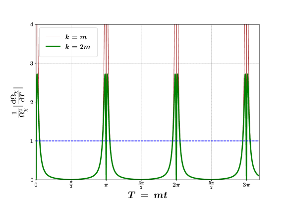
Figure 22: Violation of the adiabaticity condition, as stated in Eq. (259), is demonstrated in the broad parametric resonance regime of the Mathieu Eq. (255) with a resonance parameter $q=200$. The brown and green curves correspond to $k=m$ and $k=2m$ respectively. Particle production in the broad resonance regime takes place in the neighbourhood of $T=n\pi$ where the adiabaticity condition is violated, i.e $\frac{1}{\Omega^{2}_{\chi}}\,\Big{|}\frac{{\rm d}\Omega_{\chi}}{{\rm d}T}\Big{|}\,\geq\,1$ (for the segments of the green and brown curves above the blue dashed line).

Hence in the broad resonance regime, it is possible to produce quanta of the offspring field with momenta greater than the rest mass of the inflaton, as can be seen from Fig. 20. This non-perturbative effect is a distinctive feature of the broad parametric resonance [28].

(2) Backreaction:

The second stage witnesses the backreaction of explosively growing $\chi$ particles on the homogeneous inflaton condensate $\phi(t)$. Backreaction becomes significant when the energy density of the fluctuations becomes comparable to that of the condensate i.e., $\rho_{\chi},\rho_{\delta\varphi}\sim\rho_{\phi}$, leading to the fragmentation of the inflaton condensate. Since the coherent oscillations are hindered, parametric resonance is quenched [28] and the production of $\chi$ particles slows down appreciably.

(3) Scattering and thermalization:

In the third and final phase, the remaining inflaton condensate $\phi(t)$ decays perturbatively, leading to a large number of decay products. This in turn leads to the re-scattering off these new decay products, which further decay into the quanta of other fields that they are (very weakly) coupled to. Eventually the decay products thermalize resulting in the commencement of the familiar radiation-dominated hot Big Bang phase, acquiring a reheating temperature $T_{\rm re}$ (which is different from the result obtained in the perturbative approach given in Eq. (238)). Thus the end of the third stage leads to the commencement of the radiative hot Big Bang phase of expansion during which the EoS in the universe is $p\simeq\rho/3$. Note that the exact mechanism by which the universe thermalized after the inflaton decay is not currently known, however, see Refs. [187, 188, 189].

In the above discussion of preheating via parametric resonance, we ignored the effects of the background space which continues to expand as reheating proceeds. In practice, since $H\neq 0$, the physical momenta of the produced $\chi$ field quanta, given by $k_{p}=k/a$, get redshifted away from the broad resonance band, as shown by the white flow lines in Fig. 20. Consequently, resonant production of $\chi$ particles are quenched and the inflaton eventually proceeds to decay perturbatively. In certain cases, the effects of expansion of space leads to stochastic resonance during preheating, as discussed in Ref. [28]. However, we will not elaborate further on such complex phenomenology associated with reheating.

The dynamics of the aforementioned three stages of reheating is quite complex and usually requires a numerical treatment using lattice simulations of the full non-linear field equations [32, 190, 191]. Reheating dynamics is one of the important open problems in theoretical and observational cosmology. For a detailed account of reheating, we direct the interested readers to Ref. [31].

9 Discussions

The physics of inflation is quite broad and rich, consisting of topics ranging from fundamental physics, String Theory and UV completeness to the observational aspects of CMB and LSS. Furthermore, the inflationary cosmology involves signals in the form of primordial features such as the relic gravitational waves, primordial non-Gaussianity, primordial black holes (PBHs) etc. Additionally, a number of important topics, such as the initial conditions for inflation, eternal inflation and multiverse, loop corrections to inflationary correlators, effective field theory of inflation and alternatives to inflation, are of great interest to researchers in the field.

In these lecture notes we covered only some aspects of inflationary cosmology, although we made an attempt to be comprehensive and pedagogical in our approach to these topics. Consequently, we have left out some of the aforementioned key aspects of inflation in the present version of these lecture notes. Therefore, before concluding, we provide brief discussions on some of the important topics in inflationary cosmology that were not covered in the preceding sections.

• Relativistic cosmological perturbation theory: While computing the power spectra of inflationary scalar and tensor perturbations, we worked in the framework of gauge-invariant relativistic perturbation theory [192], and made use of a number of standard results from perturbation theory, especially in Secs. 6.2, 6.3 and 6.4. However, we did not provide a detailed introduction to the subject, for which we point the readers to Refs. [86, 132, 193, 87, 9, 88, 89, 35].

• Beyond two-point correlators – primordial non-Gaussianity: The imprints of high energy primordial interactions during inflation are encoded in the higher-order correlation functions of inflationary scalar and tensor fluctuations. This makes the study of primordial non-Gaussianity one of the most important frontiers in early universe cosmology [194, 130]. However, our treatment of the subject was minimal in Sec. 6.4. In fact, apart from the standard In-In formalism (interaction picture in QFT) [85, 195, 196, 126, 197, 128, 125], there are a number of alternate techniques to compute the higher order primordial correlators, such as the $\delta$N formalism [198, 199, 200, 201, 202, 203, 204, 205, 206, 207, 208], wave functional $\Psi[\zeta]$ approach [209, 210] and cosmological bootstrap [211, 212, 213, 214, 215, 216, 217, 218, 219, 220, 221]. A thorough account of the subject can be found in the lecture notes.

• Inflationary model building: In Sec. 7.1, we stressed that in the single field slow-roll inflationary framework, the latest CMB observations favour asymptotically flat potentials. Furthermore, in Sec. 7.2, we discussed the dynamics of a number of asymptotically flat potentials, in light of the recent observations. However, our presentation in Sec. 7 was rather phenomenological, without reference to the microphysical origin of the scalar field and its potential. Inflationary model building from the perspective of (potentially UV-complete) fundamental physics, both in the context of quantum field theory and String Theory is an important and active field of research, see Refs. [8, 222, 154].

• Effective field theory (EFT) of inflation: A convenient way to study inflationary dynamics for a large class of models in a model-independent way is the formalism of EFT applied to inflation [223, 224, 225]. Since the time-translational symmetry of pure de Sitter spacetime is spontaneously broken during inflation (in order to ensure the end of inflation), working in the unitary gauge, a general EFT can be constructed keeping the lowest dimensional operators invariant under spatial diffeomorphisms [223]. The EFT approach enables us to systematically incorporate high energy corrections to slow-roll inflationary dynamics.

• Observational probes of inflation: Since the inflationary correlators constitute one of the primary probes of ultra-high energy physics of the early universe, a plethora of precision observational missions have been dedicated to scrutinize various predictions of the inflationary scenario. This is an important topic in fundamental observational cosmology, especially in the context of CMB, galaxy clustering, and 21 cm intensity fluctuations. Since our treatment of the observational aspects of inflation in Sec. 6.5 was minimal, we direct the readers to Refs. [132, 15, 16, 33, 226, 227, 228, 229, 230, 231, 232, 35, 91] for a more elaborate discussion on the subject.

• Beyond slow-roll inflation: The latest CMB observations provide support for the single field slow-roll paradigm of inflation and favour asymptotically flat potentials, as discussed in Sec. 7.1. However, it is important to stress that the CMB and LSS observations are sensitive to the comoving wavenumbers in the range $k_{\rm CMB}\in[0.0005,0.5]\leavevmode\nobreak\ {\rm Mpc}^{-1}$, which correspond to only $7$-$8$ e-folds of accelerated expansion during inflation, and hence a relatively small region of the inflaton potential, see Fig. 8.

  On smaller scales, possible deviations from the slow-roll dynamics may lead to interesting changes in the spectra of primordial perturbations [79, 80, 81, 233]. In particular, if the scalar perturbations are sufficiently large on small scales, then Primordial Black Holes (PBHs) may form when these modes enter the Hubble radius during the post-inflationary epoch [234, 235, 236, 237, 238, 239, 240]. PBHs are therefore a powerful probe of the inflaton potential over the full range of field values. Large, potentially PBH forming, fluctuations can be generated by a feature in the inflationary potential [241, 242, 243, 244, 245, 246], such as a flat inflection point shown in Fig. 23. Such a feature can substantially slow down the already slowly rolling inflaton field, causing the inflaton to enter into an ultra slow-roll (USR) phase, which leads to an enhancement of the power spectrum, ${\cal P}_{\zeta}$, of the primordial curvature perturbations, see Refs. [79, 80, 81, 247, 82, 248, 243, 249, 250, 251, 252, 253]. Although scalar and tensor fluctuations are decoupled at linear order in perturbation theory, second-order tensor fluctuations can be sourced by the enhanced first-order scalar fluctuations and hence they are called the Scalar-induced Gravitational Waves (SIGWs). The study of enhancement of the small-scale primordial fluctuations is an active topic of research at present, especially in the context of PBH formation, since PBHs are a natural candidate for dark matter, see Refs. [254, 255, 256, 242, 257, 258, 259, 260].

  

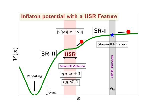
  Figure 23: A schematic illustration of a plateau potential (solid green line). The ‘CMB Window’ represents field values corresponding to cosmological scales $k_{\rm CMB}\in\left[0.0005,0.5\right]\leavevmode\nobreak\ {\rm Mpc}^{-1}$ that are probed by CMB observations. The blue star represents the CMB pivot scale $k_{*}=0.05\,{\rm Mpc}^{-1}$. The potential has a flat inflection-point like segment (highlighted with pink shading) which results in ultra slow-roll (USR) inflation. After the first slow-roll phase (SR-I) near the CMB Window, the inflaton enters into an USR phase. During this transient phase of USR, the second slow-roll condition is violated, specifically $\eta_{H}\simeq+3$. This leads to an enhancement in the primordial perturbations on small scales. Later, the inflaton emerges from the USR into another slow-roll phase (SR-II) before inflation ends at $\phi_{\rm end}$.

• Large quantum fluctuations and stochastic inflation: Under certain conditions, the comoving curvature fluctuations during inflation can be quite large, e.g. in the scenarios of eternal inflation [8, 261, 262, 263, 264, 265, 266, 123, 267, 268] (on length scales larger than $k_{\rm CMB}^{-1}$) and PBH formation (on length scales smaller than $k_{\rm CMB}^{-1}$) as discussed above. In such situations, one needs a convenient formalism to resum the non-linearities associated with the fluctuations in order to carry out the computation of inflationary correlators accurately. The stochastic inflation formalism [12, 269, 270, 271, 272, 273] is an useful approach in this direction. It is an effective treatment of the dynamics of the long-wavelength (IR) part of the inflaton field coarse-grained on scales much greater than the Hubble radius i.e. $k\leq\sigma\,aH$, with the constant $\sigma\ll 1$. In this framework, the evolution of the coarse-grained inflaton field is governed by two first-order non-linear stochastic Langevin-type differential equations which receive constant quantum kicks from the small scale UV modes that are exiting the Hubble radius due to the accelerated expansion during inflation. Hence the small-scale fluctuations constitute classical stochastic noise terms in the Langevin equations. The formalism is usually combined with the classical $\delta N$ formalism [12, 198, 98, 97, 274] in order to compute cosmological correlators in this framework. This leads to the emergence of the stochastic $\delta{\cal N}$ formalism, see Refs.  [269, 275, 276, 277, 278, 279, 83].

  Typical fluctuations, which induce temperature anisotropies in the CMB and seed the formation of large scale structure of the universe, belong to the head of the primordial PDF, which is predominantly Gaussian [85, 124, 130, 64]. However, rare fluctuations, such as those leading to eternal inflation and primordial black hole formation, belong to the tail of the PDF which is expected to be highly non-Gaussian [278, 280, 281, 123, 267, 282, 283], as illustrated schematically in Fig. 24. The tail of the primordial PDF can be determined in the framework of stochastic $\delta{\cal N}$ formalism by using the techniques of first-passage time analysis [277, 278, 280, 279, 284, 281, 279, 83, 285].

  

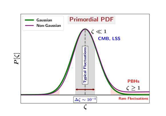
  Figure 24: A schematic illustration of the probability distribution (PDF), $P[\zeta]$, of the primordial curvature fluctuations $\zeta$. The typical fluctuations, which induce temperature fluctuations in the CMB and facilitate the formation of large scale structure of the universe, belong to the head of the primordial PDF (represented by grey colour shaded region) which is predominantly Gaussian (green colour curve). However, rare fluctuations, such as those leading to eternal inflation and primordial black hole formation, belong to the tail of the PDF (represented by pink colour shaded region) which can be highly non-Gaussian (purple colour curve).

• Multi-field inflation: In these lecture notes we primarily focused on the simplest scenario of single field inflationary dynamics. Since inflation is supposed to have taken place in the very early universe at energy scales much higher than that of the Standard Model (SM) of particle physics, it is expected to be described in the framework of beyond SM physics, such as supersymmetry, supergravity and string theory. Most beyond SM theories feature multiple scalar degrees of freedom which might have been relevant during inflation. Hence the multi-field inflationary framework have been investigated extensively over the past three decades [286, 287, 288, 289, 290, 291, 292, 293, 294, 295, 296]. They have distinctive signatures in the form of primordial non-Gaussianity and isocurvature perturbations, which make testing the multi-field inflationary scenario an important observational target for the upcoming decades [201, 297, 298, 299, 300, 301, 302, 303].

• Dissipative effects during inflation: In the standard inflationary scenario, the inflaton couplings to external fields are assumed to be very small. Particle production during inflation can be ignored because the accelerated expansion of space rapidly dilutes the number densities of the produced particles. Hence, the inflaton decay becomes significant only after the end of inflation when the expansion of space begins to decelerate, ultimately leading to reheating, as discussed in Sec. 8. However, if the inflaton couplings to other degrees of freedom are strong enough, then particle production during inflation leads to a non-negligible backreaction on the inflaton dynamics, modifying the inflationary predictions of the primordial perturbations. In general, such scenarios are collectively referred to as dissipative inflation [304, 305, 306, 307, 308, 309, 310, 311, 312, 313]. In certain regimes, the produced light degrees of freedom behave as a (sub-dominant) thermal radiation bath during inflation, leading to the emergence of warm inflation [314, 315, 316, 317, 318]. The warm inflationary paradigm exhibits certain advantages over the standard dissipationless cold inflationary paradigm from the perspective of fundamental model building as well as reheating, see Refs. [319, 320, 183].

• Initial conditions for Inflation: Our discussions in Sec. 4 stressed that once inflation begins, and lasts for a sufficiently long number of e-folds of expansion, it successfully addresses the initial conditions for the hot Big Bang phase. However, we did not make any comment on whether inflation can begin starting from generic initial conditions in the pre-inflationary universe, closer to the Planck scale. In fact, the investigation of initial conditions for inflation is an important conceptual exercise, and there has been a great deal of research work on the topic, both analytically and computationally, see Refs. [74, 33, 9, 75, 76, 77, 321, 322, 323, 324, 325, 65, 326, 67, 327, 328, 329, 330, 331].

• Alternatives to inflation: While cosmic inflation is certainly the leading scenario in explaining the initial conditions for the hot Big Bang, there exit a number of alternatives to inflation [332, 333, 334, 335, 336, 337] which can also address the initial conditions, and are consistent with the observations of primordial perturbations at present. Amongst these are the matter bounce scenario [338, 339, 340], pre-Big Bang and the ekpyrotic cosmology [341, 342, 343, 344, 345, 346, 347, 348], and emergent string gas cosmology [349, 350, 351], to mention a few. However, many of the future observational probes will be dedicated to provide a decisive direction, either for, or against the inflationary paradigm, see Refs. [15, 16, 352, 353, 354, 355, 356].

10 Supplementary sources

There exist a number of excellent sources (lecture notes/reviews) in the literature on cosmic inflation. In the following, I refer to some of the sources that I have personally found useful over the years.

1. I originally learned inflation from three sources: (i) Handwritten lecture notes by Paolo Creminelli given at ICTP in 2013/14, (ii) a set of lectures on inflation given by Nima Arkani-Hamed (link to the videos) and Juan Maldacena (link to the videos) at the ICTP Spring School in 2014, and finally (iii) ‘TASI Lectures on Inflation’ by Daniel Baumann in Ref. [9].

2. Lecture notes on ‘Inflation and the theory of cosmological perturbations’ by Antonio Riotto in Ref. [103].

3. ‘TASI lectures on Inflation’ by William Kinney in Ref. [100].

4. Lecture notes titled ‘An introduction to inflation and cosmological perturbation theory’ by L. Sriramkumar in Ref. [90].

5. TASI ‘Lectures on Inflation’ by Leonardo Senatore in Ref. [225].

6. Standard cosmology textbooks such as the ‘Physical Foundations of Cosmology’ by Mukhanov [33], ‘Introduction to the theory of the early universe: Cosmological perturbations and inflationary theory’ by Gorbunov and Rubakov [89] and ‘Cosmology’ by Daniel Baumann [35].

7. ‘TASI lectures on Primordial Cosmology’ by Daniel Baumann in Ref. [91] which have been quite useful to me in the past few years.

8. A set of lectures on inflation by Matthew Kleban at the ICTP Summer School 2018 (link to the YouTube playlist).

9. ‘Lectures on Cosmological Correlations’ by Daniel Baumann and Austin Joyce, given in the github link, covering more recent developments in the field.

Appendices

Appendix A Hubble parameter in the early universe

The early universe is assumed to be thermal and radiation dominated, at least up to a temperature of $T_{\rm EW}\sim 200\leavevmode\nobreak\$GeV. The radiation density of the thermal plasma is given by

$$\rho_{r}(T)=\frac{\pi^{2}}{30}\,g_{*}(T)\,T^{4},$$ (260)

where, $g_{*}(T)$ is the effective number of relativistic degrees of freedom in the energy density at temperature $T$. In the flat ${\rm\Lambda}$CDM model, matter, radiation and dark energy evolve without interacting with each other at lower redshifts (late times). However, that was not the case in the very early universe. Due to the presence of high density and temperature conditions, the universe was in an extremely hot and dense plasma state. Hence the rate of interactions were higher, and matter and radiation could convert into each other more easily. Since entropy is conserved for a thermal distribution, keeping track of the entropy is quite useful in determining the evolution of radiation density and temperature in the hot Big Bang phase. Using the conservation of entropy [24],

$$S_{0}=S_{T},$$ (261)

where, $S_{0}$ is the entropy today and $S_{T}$ is the entropy measured at some temperature T in the past. This leads to

$$s_{0}\,a_{0}^{3}=s_{T}\,a^{3},$$ (262)

where $s$ is the entropy density given by

$$s=\frac{2\pi^{2}}{45}\,g^{s}_{*}(T)\,T^{3}\,,$$

and $g^{s}_{*}$ is the effective number of relativistic degrees of freedom in the entropy density. Hence, Eq. (262) can be written as

$$\frac{2\pi^{2}}{45}\,T_{0}^{3}\,g^{s}_{0,*}\,a_{0}^{3}=\frac{2\pi^{2}}{45}\,{T^{3}}\,g^{s}_{*}\,{a}^{3}\,,$$

yielding

$$\boxed{T=\left(\frac{g^{s}_{0,*}}{g^{s}_{*}}\right)^{1/3}\,\left(\frac{a_{0}}{a}\right)\,T_{0}=\left(\frac{g^{s}_{0,*}}{g^{s}_{*}}\right)^{1/3}\,\left(1+z\right)\,T_{0}}\,.$$ (263)

Inserting Eq. (263) into Eq. (260), we obtain the expression for the radiation energy density at any given redshift $z$ to be

$$\rho_{r}(T)=\frac{\pi^{2}}{30}\,g_{*}(T)\,\left(\frac{g^{s}_{0,*}}{g^{s}_{*}}\right)^{4/3}\,(1+z)^{4}\,T_{0}^{4}\,,$$ (264)

while the radiation energy density at the present epoch is given by

$$\rho_{0r}=\frac{\pi^{2}}{30}\,g_{0,*}\,T_{0}^{4}\,.$$ (265)

Accordingly, using the Friedmann Eq. (6) with $K=0$, we obtain the expression for the Hubble parameter as a function of redshift in the radiation dominated epoch to be

$$\boxed{H(z)\simeq H_{0}\,\left(\Omega_{0r}\,\frac{g_{*}}{g_{0,*}}\right)^{1/2}\,\left(\frac{g^{s}_{0,*}}{g^{s}_{*}}\right)^{2/3}\,(1+z)^{2}}\,.$$ (266)

Appendix B Kinematics of reheating and the duration of inflation

The epoch of reheating is usually characterized by a set of three parameters $\{w_{{}_{\rm re}},N_{{}_{\rm re}},T_{{}_{\rm re}}\}$, namely, the effective equation of state (EoS) during reheating $w_{{}_{\rm re}}$, the duration of reheating $N_{{}_{\rm re}}$ and the temperature at the end of reheating $T_{{}_{\rm re}}$, when the universe transits to a thermalized radiation dominated hot Big Bang phase. The duration of reheating can be defined by the number of $e$-folds of expansion between the end of inflation $a_{e}$ and the end of reheating (or equivalently, the commencement of radiation domination) $a_{re}$, given by

$$N_{{}_{\rm re}}=\ln\left(\frac{a_{\rm re}}{a_{e}}\right)\,.$$ (267)

While $N_{{}_{\rm re}}$ and $T_{{}_{\rm re}}$ are interesting physical quantities, in their own right, describing the epoch of reheating, they are also potentially important for correctly interpreting the bounds on the CMB observables such as the scalar spectral index $n_{{}_{S}}$ and the tensor-to-scalar ratio $r$.

Following the evolution of the comoving Hubble radius from the epoch of Hubble-exit, at $a=a_{k}$, of a comoving scale $k$, through its post-inflationary Hubble-entry at $a=a_{p}$, until the present epoch $a=a_{0}$, we obtain

$$\ln{\left(\frac{k}{a_{0}H_{0}}\right)}=-N_{k}^{\rm inf}-N_{{}_{\rm re}}-N_{{}_{\rm RD}}-\ln{\left(1+z_{\rm eq}\right)}+\ln{\frac{H_{k}^{\rm inf}}{H_{0}}}\leavevmode\nobreak\ ,$$ (268)

where $H_{k}^{\rm inf}$ is the Hubble parameter at the time of the Hubble-exit of the scale $k$, $N_{k}^{\rm inf}=\ln{\left(a_{e}/a_{k}\right)}$ is the number of $e$-folds between the Hubble-exit (of scale $k$) and the end of inflation, $N_{{}_{\rm RD}}$ is the duration of the radiation dominated epoch and $z_{\rm eq}$ is the redshift at the epoch of matter-radiation equality. In general, $k$ may correspond to any observable CMB scale in the range $k\in\left[0.0005,0.5\right]\leavevmode\nobreak\ {\rm Mpc}^{-1}$. The CMB pivot scale, namely $k\equiv k_{*}=0.05\leavevmode\nobreak\ {\rm Mpc}^{-1}$, makes its Hubble-entry during the radiative epoch at $a_{p}\sim 4\times 10^{-5}\,a_{0}$, see Fig. 25.

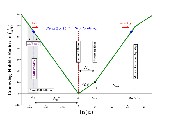
Figure 25: Schematic illustration of the evolution of the comoving Hubble radius $(aH)^{-1}$ with scale factor. During inflation $(aH)^{-1}$ decreases which causes physical scales to exit the Hubble radius. After inflation ends $(aH)^{-1}$ increases, and physical scales begin to enter the Hubble radius. The CMB pivot scale, as used by the Planck mission, is set at $k_{*}=0.05\leavevmode\nobreak\ {\rm Mpc}^{-1}$. It enters the Hubble radius during the radiation dominated epoch when $a_{p}\sim 4\times 10^{-5}\,a_{0}$. Note that the duration of reheating $N_{{}_{\rm re}}$, and hence the duration of the radiation dominated epoch $N_{{}_{\rm RD}}$, changes for different values of the reheating equation of state $w_{{}_{\rm re}}$. Recall that $(aH)^{-1}\propto a$ during the radiative regime and $(aH)^{-1}\propto a^{-1}$ during inflation.

The primary goal here is to characterize the epoch of reheating between the end of inflation $a_{e}$ and the commencement of the radiative epoch $a_{\rm re}$. Assuming the effective EoS $w_{{}_{\rm re}}$ during reheating to be a constant allows us to match the density at the beginning of the radiative epoch to the density at the end of inflation by

$$\rho_{{}_{\rm re}}=\rho_{e}\left(\frac{a_{e}}{a_{\rm re}}\right)^{3(1+w_{{}_{\rm re}})}\leavevmode\nobreak\ ,$$ (269)

which yields the following expression for the duration of reheating [145]:

$$N_{{}_{\rm re}}\equiv\ln{\left(\frac{a_{\rm re}}{a_{e}}\right)}=\frac{1}{3(1+w_{{}_{\rm re}})}\ln{\left(\frac{\rho_{e}}{\rho_{{}_{\rm re}}}\right)}\leavevmode\nobreak\ .$$ (270)

Expressing $\rho_{{}_{\rm re}}$ in terms of the reheating temperature $T_{{}_{\rm re}}$, we obtain

$$N_{{}_{\rm re}}=\frac{1}{3(1+w_{{}_{\rm re}})}\ln{\left(\frac{\rho_{e}}{\frac{\pi^{2}}{30}\,g_{\rm re}T_{{}_{\rm re}}^{4}}\right)}\leavevmode\nobreak\ ,$$ (271)

where $g_{\rm re}\equiv g(T_{{}_{\rm re}})$ is the effective number of relativistic degrees of freedom at the end of reheating. Applying entropy conservation, as discussed in App. A, to express $T_{{}_{\rm re}}$ in terms of $a_{\rm re}$, we obtain

$$T_{{}_{\rm re}}=\left(\frac{g_{\rm eq}^{s}}{g_{\rm re}^{s}}\right)^{\frac{1}{3}}\left(\frac{a_{\rm eq}}{a_{\rm re}}\right)T_{\rm eq}\leavevmode\nobreak\ ,$$ (272)

where $g_{\rm eq}^{s}$ and $g_{\rm re}^{s}$ are the effective number of relativistic degrees of freedom in the entropy at the epoch of matter-radiation equality and at the end of reheating respectively, while $T_{\rm eq}$ is the temperature at the matter-radiation equality. Incorporating (272) into (271), we obtain (see Ref. [145])

$$N_{{}_{\rm re}}=\frac{4}{3(1+w_{{}_{\rm re}})}\left[\frac{1}{4}\ln{\left(\frac{30}{\pi^{2}g_{\rm re}}\right)}+\frac{1}{3}\ln{\left(\frac{g_{\rm re}^{s}}{g_{\rm eq}^{s}}\right)}+\ln{\left(\frac{\rho_{e}^{\frac{1}{4}}}{T_{\rm eq}}\right)}-N_{{}_{\rm RD}}\right]\leavevmode\nobreak\ .$$ (273)

Substituting $N_{{}_{\rm RD}}$ from (268) into (273), we arrive at an important expression for the duration of reheating, namely (see Ref. [145])

$$N_{{}_{\rm re}}=\frac{4}{3(1+w_{{}_{\rm re}})}\left[\frac{1}{4}\ln{\left(\frac{30}{\pi^{2}g_{\rm re}}\right)}+\frac{1}{3}\ln{\left(\frac{g_{\rm re}^{s}}{g_{0}^{s}}\right)}+\ln{\left(\frac{\rho_{e}^{\frac{1}{4}}}{H_{k}^{\rm inf}}\right)}+\ln{\left(\frac{k}{a_{0}T_{0}}\right)}+N_{k}^{\rm inf}+N_{{}_{\rm re}}\right]\leavevmode\nobreak\ .$$ (274)

Note that if $w_{{}_{\rm re}}=1/3$, then the term $N_{{}_{\rm re}}$ cancels from both sides of (274), yielding the following expression for $N_{k}^{\rm inf}$

$$N_{k}^{\rm inf}=-\left[\ln{\left(\frac{k}{a_{0}T_{0}}\right)}+\ln{\left(\frac{\rho_{e}^{\frac{1}{4}}}{H_{k}^{\rm inf}}\right)}+\frac{1}{4}\ln{\left(\frac{30}{\pi^{2}g_{\rm re}}\right)}+\frac{1}{3}\ln{\left(\frac{g_{\rm re}^{s}}{g_{0}^{s}}\right)}\right]\leavevmode\nobreak\ .$$ (275)

This arises because the end of reheating, and hence the beginning of the radiative epoch, cannot be strictly defined within this framework if $w_{{}_{\rm re}}=1/3$. However for $w_{{}_{\rm re}}\neq 1/3$ one obtains the following final expression for $N_{{}_{\rm re}}$ from Eq. (274)

$$N_{{}_{\rm re}}=-\frac{4}{1-3w_{{}_{\rm re}}}\left[N_{k}^{\rm inf}+\ln{\left(\frac{\rho_{e}^{\frac{1}{4}}}{H_{k}^{\rm inf}}\right)}+\ln{\left(\frac{k}{a_{0}T_{0}}\right)+\frac{1}{4}\ln{\left(\frac{30}{\pi^{2}g_{\rm re}}\right)}+\frac{1}{3}\ln{\left(\frac{g_{\rm re}^{s}}{g_{0}^{s}}\right)}}\right]\leavevmode\nobreak\ .$$ (276)

Accordingly the expression for the reheating temperature $T_{{}_{\rm re}}$ in terms of the duration of reheating $N_{{}_{\rm re}}$ and effective reheating EoS, $w_{{}_{\rm re}}$, follows from (271) to be

$$T_{{}_{\rm re}}=\left(\frac{30\rho_{e}}{\pi^{2}g_{\rm re}}\right)^{\frac{1}{4}}e^{-\frac{3}{4}\left(1+w_{{}_{\rm re}}\right)N_{{}_{\rm re}}}\leavevmode\nobreak\ .$$ (277)

Note that the expressions (276) and (277) are valid only for $w_{{}_{\rm re}}\neq 1/3$. We return to the case $w_{{}_{\rm re}}=1/3$ at the end of this subsection, for which the relevant final expression for $N_{k}^{\rm inf}$, following Eq. (275), is given in Eq. (282).

In the context of single field slow-roll inflation, the value of the inflaton field at the end of inflation $\phi_{e}$ can be determined from the condition

$$\epsilon_{{}_{V}}(\phi_{e})=\frac{m_{\rm p}^{2}}{2}\left(\frac{V_{,\phi}}{V}\right)^{2}\bigg{|}_{\phi_{e}}\simeq 1\leavevmode\nobreak\ ,$$ (278)

and the corresponding inflaton density at the end of inflation is given by

$$\rho_{e}\equiv\rho_{\phi}\bigg{|}_{\phi_{e}}=\frac{1}{2}\dot{\phi}^{2}+V(\phi)\bigg{|}_{\phi_{e}}\simeq\frac{3}{2}V(\phi_{e})\equiv\frac{3}{2}V_{e}\leavevmode\nobreak\ .$$

Substituting $\rho_{e}=\frac{3}{2}V_{e}$ in (277) results in the following expression for the reheating temperature

$$T_{{}_{\rm re}}=\left(\frac{45}{\pi^{2}g_{\rm re}}\right)^{\frac{1}{4}}V_{e}^{\frac{1}{4}}\,e^{-\frac{3}{4}\left(1+w_{{}_{\rm re}}\right)N_{{}_{\rm re}}}\leavevmode\nobreak\ .$$ (279)

Assuming $k$ to be the CMB pivot scale, $k\equiv k_{*}=a_{k}H_{k}^{\rm inf}=a_{p}H_{p}=0.05\leavevmode\nobreak\ {\rm Mpc}^{-1}$ in (276) and inserting the values of $T_{0}$, $g_{0}^{s}$, $g_{\rm re}$ and $g_{\rm re}^{s}$, one arrives at the following formula which expresses the duration of reheating $N_{{}_{\rm re}}$ as a function of the reheating EoS, $w_{{}_{\rm re}}$, on the one hand, and parameters of the inflationary potential $V_{e}$, $H_{k}^{\rm inf}$, on the other:

$$N_{{}_{\rm re}}=\frac{4}{1-3w_{{}_{\rm re}}}\left[61.55-N_{k}^{\rm inf}-\ln{\left(\frac{V_{e}^{\frac{1}{4}}}{H_{k}^{\rm inf}}\right)}\right]\leavevmode\nobreak\ ,\leavevmode\nobreak\ \leavevmode\nobreak\ \leavevmode\nobreak\ \leavevmode\nobreak\ w_{{}_{\rm re}}\neq 1/3.$$ (280)

Eqs. (280) and (279) capture some of the essential implications of reheating kinematics on CMB observables and possess important physical significance. For example, it is easy to see, from Eq. (280), that for a softer reheating EoS with $w_{{}_{\rm re}}<1/3$, a higher value of $N_{k}^{\rm inf}$ corresponds to a shorter reheating period $N_{{}_{\rm re}}$, for a given model of inflation. Exactly the opposite is true for a stiffer EoS with $w_{{}_{\rm re}}>1/3$. In this case the RHS of Eq. (280) flips sign so that a larger value of $N_{k}^{\rm inf}$ implies a larger $N_{{}_{\rm re}}$ and hence a longer duration of reheating. Similarly Eq. (279) implies that the longer is the duration of reheating $N_{{}_{\rm re}}$, the lower will be the reheating temperature $T_{{}_{\rm re}}$. Moreover this result is independent of the value of $w_{{}_{\rm re}}$ simply because $1+w_{{}_{\rm re}}>0$ (since $w_{{}_{\rm re}}>-1/3$ by definition). Another interesting aspect of Eq. (280) is that, given an inflationary potential with a fixed value of $N_{k}^{\rm inf}$ (which satisfies the CMB bound on $n_{{}_{S}}\in\left[0.957,0.976\right]$), the duration of reheating $N_{{}_{\rm re}}$ increases with an increase in the effective EoS $w_{{}_{\rm re}}$ as long as $w_{{}_{\rm re}}<1/3$. This is demonstrated in the left panel of Fig. 26 in which $N_{{}_{\rm re}}^{(1)}<N_{{}_{\rm re}}^{(2)}$ for $w_{{}_{\rm re}}^{(1)}<w_{{}_{\rm re}}^{(2)}<1/3$. Similarly $N_{{}_{\rm re}}$ increases with a decrease in the effective EoS, $w_{{}_{\rm re}}$, if $w_{{}_{\rm re}}>1/3$. This is shown in the right panel of fig. 26 where $N_{{}_{\rm re}}^{(1)}<N_{{}_{\rm re}}^{(2)}$ for $w_{{}_{\rm re}}^{(1)}>w_{{}_{\rm re}}^{(2)}>1/3$. These arguments also indicate that $w=1/3$ is a critical value of the EoS during reheating.

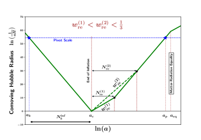
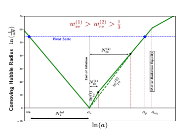
Figure 26: This figure schematically illustrates the evolution of the comoving Hubble radius $(aH)^{-1}$ with scale factor of the universe and explicitly depicts the dependence of the duration of reheating on the reheating equation of state for a particular inflationary model with a given $N_{k}^{\rm inf}$. The left panel shows that for shallow reheating EoS $w_{{}_{\rm re}}<1/3$, the duration of reheating $N_{{}_{\rm re}}$ is longer for a higher value of $w_{{}_{\rm re}}$, namely $N_{{}_{\rm re}}^{(1)}<N_{{}_{\rm re}}^{(2)}$ for $w_{{}_{\rm re}}^{(1)}<w_{{}_{\rm re}}^{(2)}$. The right panel demonstrates that for a stiffer reheating EoS $w_{{}_{\rm re}}>1/3$, the duration of reheating $N_{{}_{\rm re}}$ is shorter for a higher value of $w_{{}_{\rm re}}$, namely $N_{{}_{\rm re}}^{(1)}<N_{{}_{\rm re}}^{(2)}$ for $w_{{}_{\rm re}}^{(1)}>w_{{}_{\rm re}}^{(2)}$, in accordance with equation (280). Note that $(aH)^{-1}\propto a$ during the radiative regime and $(aH)^{-1}\propto a^{-1}$ during inflation. For comparison see Fig. 25.

Turning attention to $T_{{}_{\rm re}}$, one notes that conservative upper and lower bounds on this quantity can be placed from the following considerations. In Sec. 7.1, we learned that the CMB upper bound on the tensor-to-scalar ratio, namely $r\leq 0.036$, translates into an upper bound on the inflationary Hubble scale $H_{k}^{\rm inf}\leq 4.7\times 10^{13}\leavevmode\nobreak\ {\rm GeV}$, which in turn sets an upper bound on the energy scale of inflation $T_{\inf}\leq 1.4\times 10^{16}\leavevmode\nobreak\ {\rm GeV}$. Since reheating happens after the end of inflation, one gets $T_{{}_{\rm re}}\leq 1.4\times 10^{16}\leavevmode\nobreak\ {\rm GeV}$ as an absolute upper bound on the reheating temperature. Similarly, in order to preserve the success of the hot Big Bang phase, reheating must terminate before the beginning of Big Bang Nucleosynthesis (BBN) yielding the absolute lower bound $T_{{}_{\rm re}}\gg 1\leavevmode\nobreak\ {\rm MeV}$. Hence the most conservative bounds on the reheating temperature are

$$1\,{\rm MeV}\ll T_{{}_{\rm re}}\leq 10^{16}\,{\rm GeV}\,.$$ (281)

Note that Eq. (280) is only applicable for reheating EoS with $w_{{}_{\rm re}}\neq 1/3$. For $w_{{}_{\rm re}}=1/3$, using Eq. (275), assuming $k$ to be the CMB pivot scale, i.e $k\equiv k_{*}=0.05\leavevmode\nobreak\ {\rm Mpc}^{-1}$ and inserting the values of $T_{0}$, $g_{0}^{s}$, $g_{\rm re}$ and $g_{\rm re}^{s}$, as was previously done for the case $w_{{}_{\rm re}}\neq 1/3$, one obtains the following strong prediction for $N_{k}^{\rm inf}$.

$$N_{k}^{\rm inf}=61.55-\ln{\left(\frac{V_{e}^{\frac{1}{4}}}{H_{k}^{\rm inf}}\right)}\,.$$ (282)

Since $H_{e}^{\rm inf}=\sqrt{3m_{p}^{2}\,V_{e}}$, Eq. (282) becomes

$$N_{k}^{\rm inf}=61.3-\frac{1}{2}\,\ln{\left[\frac{H_{e}\,m_{p}}{\left(H_{k}^{\rm inf}\right)^{2}}\right]}\,.$$ (283)

For the standard quasi-dS inflation, since $H_{e}\simeq H_{k}^{\rm inf}$, we obtain the final expression

$$\boxed{N_{k}^{\rm inf}=61.3-\frac{1}{2}\,\ln{\left(\frac{m_{p}}{H_{k}^{\rm inf}}\right)}}\,,$$ (284)

which results in

$$N_{k}^{\rm inf}=\begin{cases}55.5\,;&H_{k}^{\rm inf}=2.4\times 10^{13}\,{\rm GeV}\,,\\ 52.1\,;&H_{k}^{\rm inf}=2.4\times 10^{10}\,{\rm GeV}\,,\\ 48.6\,;&H_{k}^{\rm inf}=2.4\times 10^{7}\,{\rm GeV}\,.\end{cases}$$ (285)

If reheating lasts longer with an EoS $w_{{}_{\rm re}}\neq 1/3$, then $N_{k}^{\rm inf}$ would span a larger range.

Appendix C Inflaton-clock dynamics: Hamilton-Jacobi formalism

In the standard scenario of single field slow-roll inflation, the inflaton field $\phi$ evolves monotonically during inflation. Hence, one can use $\phi$ as a clock to describe the dynamics of the background spacetime. This $\phi$-clock evolution is particularly useful in obtaining the functional form of the potential $V(\phi)$, given an inflationary evolution $H(t)$, or vice versa.

In order to achieve this, let us convert the time variable in the Friedmann equations from cosmic time $t$ to the inflaton clock time $\phi$. From Eq. (63), we get

$$\dot{H}\equiv\frac{{\rm d}H}{{\rm d}\phi}\,\dot{\phi}=-\frac{1}{2m_{p}^{2}}\,\dot{\phi}^{2}\,,$$

leading to

$$\left(\frac{{\rm d}H}{{\rm d}\phi}\right)^{2}=\frac{\dot{\phi}^{2}}{4\,m_{p}^{4}}\,.$$ (286)

Replacing the value of $\dot{\phi}^{2}$ from Eq. (62), we obtain

$$\boxed{\leavevmode\nobreak\ \left(\frac{{\rm d}H}{{\rm d}\phi}\right)^{2}\leavevmode\nobreak\ =\leavevmode\nobreak\ \frac{3}{2}\,\left[\frac{H(\phi)}{m_{p}}\right]^{2}-\,\frac{1}{2}\,\frac{V(\phi)}{m_{p}^{4}}\leavevmode\nobreak\ }\,,$$ (287)

known as the Hamilton-Jacobi equation which is a first-order non-linear ordinary differential equation that describes the evolution of $H(\phi)$ during inflation for a given potential $V(\phi)$. The corresponding expressions for the slow-roll parameters $\epsilon_{H},\,\eta_{H}$ becomes

$$\epsilon_{H} = 2\,m_{p}^{2}\,\left(\frac{H_{,\phi}}{H}\right)^{2}\,,$$ (288)

$$\eta_{H} = 2\,m_{p}^{2}\,\left(\frac{H_{,\phi\phi}}{H}\right)\,.$$ (289)

The Hamilton-Jacobi formalism has a number of important applications in inflationary cosmology. In particular, it is a convenient way to demonstrate that the slow-roll trajectory given in Eq. (75) is a local attractor, see Refs. [78, 9]. Another important application of Eq. (287) is to determine the functional form of $V(\phi)$ which leads to a particular expansion history $H(t)$ during inflation [357], as mentioned before. Let us proceed to demonstrate this for power-law inflation.

In Sec. 5.1 we discussed inflation in the quasi-de Sitter paradigm where the expansion of space was nearly exponential, $a(t)\propto a^{Ht}$. However, it is also possible to realise inflationary expansion which is not exponential. A key example of such a non-exponential inflation is the so called power-law inflation where the scale factor of the universe evolves as a monomial or power-law function of time, namely

$$a(t)\propto t^{p}\,;\quad{\rm with}\quad p>1\leavevmode\nobreak\ \leavevmode\nobreak\ \Rightarrow\leavevmode\nobreak\ \leavevmode\nobreak\ H(t)=\frac{p}{t}\,.$$ (290)

Since $p>1$, we have $\ddot{a}>0$, leading to accelerated expansion or inflation. We are then interested in determining the functional form of $V(\phi)$ which facilitates such a power-law expansion of space. To determine $V(\phi)$, we first replace the time dependence of $H$ with the $\phi$ dependence via the following steps. Using Eq. (63) and (290), we get

$$\dot{\phi}^{2}\equiv-2\,m_{p}^{2}\,\dot{H}=\frac{2p\,m_{p}^{2}}{t^{2}}\,,$$

which leads to

$$\frac{\phi(t)}{m_{p}}=\sqrt{2p}\,\ln\left(\frac{t}{t_{1}}\right)\,,$$

where $t_{1}$ is an integration constant. By inverting the above expression, we obtain cosmic time in terms of $\phi$ to be

$$t=t_{1}\,e^{\frac{1}{\sqrt{2p}}\,\frac{\phi}{m_{p}}}\,.$$ (291)

Incorporating this into the expression for $H(t)$ in Eq. (290), we obtain the final expression for the Hubble parameter and its derivative in terms of $\phi$-clock to be

$$H(\phi) = H_{1}\,e^{-\frac{1}{\sqrt{2p}}\,\frac{\phi}{m_{p}}}\,,$$ (292)

$$H_{,\phi}(\phi) = -\frac{1}{\sqrt{2p}}\,\left(\frac{H_{1}}{m_{p}}\right)\,e^{-\frac{1}{\sqrt{2p}}\,\frac{\phi}{m_{p}}}\,,$$ (293)

where $H_{1}=p/t_{1}$. The expression for the scalar field potential $V(\phi)$ from the Hamilton-Jacobi Eq. (287) is given by

$$\boxed{\leavevmode\nobreak\ \frac{V(\phi)}{m_{p}^{4}}\leavevmode\nobreak\ =\leavevmode\nobreak\ 3\,\left[\frac{H(\phi)}{m_{p}}\right]^{2}-2\,\left(\frac{{\rm d}H}{{\rm d}\phi}\right)^{2}\leavevmode\nobreak\ }\,,$$ (294)

which, using Eq. (293), becomes

$$\boxed{V(\phi)=V_{0}\,e^{-\lambda\,\frac{\phi}{m_{p}}}}\,,$$ (295)

with

$$V_{0}=\left(3-\frac{1}{p}\right)\left(\frac{H_{1}}{m_{p}}\right)^{2}\,m_{p}^{4}\,,\quad\boxed{\lambda\,=\,\sqrt{\frac{2}{p}}}\,.$$ (296)

Power-law inflation was amongst the earliest studied inflationary models, see Ref. [358]. Unfortunately, their slow-roll predictions for $\{n_{{}_{S}},\,r\}$ do not satisfy the CMB constraints, as can be seen from the purple colour curve in Fig. 14.

From the above analysis, we conclude that an exponential potential leads to the power-law expansion of space. Since we did not make use of the fact that $p>1$, the conclusion can be extended to decelerated expansion of space for $p<1$. In fact exponential potentials play an important roll in the post-inflationary scalar field dynamics. They appear in String Theory [359] and have interesting tracker properties [360] in the presence of a dominant background matter-energy component with EoS $w_{B}$, provided they are steep enough, i.e. $\lambda^{2}>3(1+w_{B})$. Consequently, they have been used extensively both in the context of dark energy [361, 362] and dark matter [363] with appropriate modifications.

Appendix D Mukhanov-Sasaki equation for scalar fluctuations

In this Appendix we outline the derivation of the Mukhanov-Sasaki equation, first in the comoving gauge and then in the spatially flat gauge. Starting from the action of a canonical scalar field minimally coupled to gravity

$$S[g_{\mu\nu},\varphi]=\int\,{\rm d}^{4}x\,\sqrt{-g}\,\left(\,\frac{m_{p}^{2}}{2}\,R-\frac{1}{2}\,\partial_{\mu}\varphi\,\partial_{\nu}\varphi\,g^{\mu\nu}-V(\varphi)\right)\leavevmode\nobreak\ ,$$

we consider linear field fluctuations $\varphi(t,\vec{x})=\phi(t)+\delta\varphi(t,\vec{x})$ and the linearly perturbed ADM metric of the form [84, 85]

$${\rm d}s^{2}=-\alpha^{2}\,{\rm d}t^{2}+\gamma_{ij}\left({\rm d}x^{i}+\beta^{i}\,{\rm d}t\right)\left({\rm d}x^{j}+\beta^{j}\,{\rm d}t\right)\,,$$

where $\alpha=1+\delta\alpha$ and $\beta^{i}$ are the lapse and shift functions, which appear as Lagrange multipliers in the perturbed action. However, $\gamma_{ij}$ are the dynamical metric perturbations in the ADM formalism.

D.1 Comoving gauge

In the comoving gauge in which inflaton fluctuations vanish, we have

$$\delta\varphi(t,\vec{x})=0\,;\quad\gamma_{ij}(t,\vec{x})=a^{2}\bigl{[}\bigl{(}1+2\,\zeta(t,\vec{x})\bigr{)}\,\delta_{ij}\,+\,h_{ij}(t,\vec{x})\bigr{]}\,.$$

By varying the perturbed action w.r.t the lapse and shift, we obtain the GR momentum and Hamiltonian constraints (see Refs. [85, 91]) to be

$$\delta\alpha=\frac{\dot{\zeta}}{H}\,;\leavevmode\nobreak\ \leavevmode\nobreak\ \leavevmode\nobreak\ \leavevmode\nobreak\ \partial_{i}\beta^{i}=-\frac{\partial^{2}\zeta}{H}+\frac{1}{2}\,a^{2}\left(\frac{\dot{\phi}^{2}}{H^{2}}\right)\,\dot{\zeta}\,.$$ (297)

Incorporating the above expressions into the action, expanding around the background, the quadratic action for $\zeta$ becomes [85, 91]

$$S^{(2)}[\zeta]=\int{\rm d}t\,{\rm d}^{3}\vec{x}\leavevmode\nobreak\ \leavevmode\nobreak\ a^{3}\,\epsilon_{H}\,\left[\,\dot{\zeta}^{2}-\left(\frac{\partial_{i}\zeta}{a}\right)^{2}\,\right]\,,$$ (298)

which, in terms of conformal time $\tau$, takes the form

$$S^{(2)}[\zeta]=\frac{1}{2}\int{\rm d}\tau\,{\rm d}^{3}\vec{x}\leavevmode\nobreak\ 2\,a^{2}\,m_{p}^{2}\,\epsilon_{H}\,\left[(\zeta^{\prime})^{2}-(\partial_{i}\zeta)^{2}\right]\,.$$

With the change of variable $v=am_{p}\sqrt{2\epsilon_{H}}\,\zeta$, the Fourier modes $v_{k}$ satisfy the Mukhanov-Sasaki equation

$$v_{k}^{\prime\prime}+\left[k^{2}+{\cal M}_{\rm eff}^{2}(\tau)\right]\,v_{k}=0\leavevmode\nobreak\ ,$$

with

$${\cal M}_{\rm eff}^{2}(\tau)=-\frac{\left(a\,m_{p}\,\sqrt{2\epsilon_{H}}\right)^{\prime\prime}}{a\,m_{p}\,\sqrt{2\epsilon_{H}}}=-(aH)^{2}\left[2+2\epsilon_{H}-3\eta_{H}+2\epsilon_{H}^{2}+\eta_{H}^{2}-3\epsilon_{H}\eta_{H}-\frac{1}{aH}\,\eta^{\prime}_{H}\right]\,.$$ (299)

D.2 Spatially flat gauge

In the spatially flat gauge

$$\gamma_{ij}(t,\vec{x})=a^{2}(t)\bigl{[}\delta_{ij}\,+\,h_{ij}(t,\vec{x})\bigr{]}\,.$$

Imposing the GR momentum and Hamiltonian constraints, one obtains (see Ref. [85])

$$\delta\alpha=\sqrt{\frac{\epsilon_{H}}{2}}\,\frac{\delta\varphi}{m_{p}}\,;\leavevmode\nobreak\ \leavevmode\nobreak\ \leavevmode\nobreak\ \leavevmode\nobreak\ \partial_{i}\beta^{i}=-\epsilon_{H}\,\frac{{\rm d}}{{\rm d}t}\left(\frac{1}{\sqrt{2\epsilon_{H}}}\,\frac{\delta\varphi}{m_{p}}\right)\leavevmode\nobreak\ .$$

Incorporating the above expressions into the action, expanding around the background, the quadratic action for $\delta\varphi$ fluctuations becomes [85, 91]

$$S^{(2)}[\delta\varphi]=\frac{1}{2}\,\int\,{\rm d}t{\rm d}^{3}{\vec{x}}\leavevmode\nobreak\ a^{3}\left[\delta\dot{\varphi}^{2}-\frac{(\partial_{i}\delta\varphi)^{2}}{a^{2}}-\left(\frac{{\rm d}^{2}V(\phi)}{{\rm d}\phi^{2}}+2\,\epsilon_{H}\,H^{2}\,\left(2\,\eta_{H}-\epsilon_{H}-3\right)\right)\delta\varphi^{2}\right]\,.$$ (300)

The Euler-Lagrange equation for $\delta\varphi$ is given by

$$\delta\ddot{\varphi}+3\,H\,\delta\dot{\varphi}-\frac{\nabla^{2}}{a^{2}}\,\delta\varphi-a^{2}H^{2}\left(2-\epsilon_{H}-\frac{1}{H^{2}}\,\frac{{\rm d}^{2}V(\phi)}{{\rm d}\phi^{2}}-\frac{2\dot{\phi}}{m_{p}^{2}H^{3}}\,\frac{{\rm d}V(\phi)}{{\rm d}\phi}-\frac{\dot{\phi}^{2}}{m_{p}^{4}H^{4}}\,V\right)\,\delta\varphi=0\leavevmode\nobreak\ .$$ (301)

With the change of variable $v=a\,\delta\varphi$, the Fourier modes $v_{k}$ satisfy the Mukhanov-Sasaki equation

$$v_{k}^{\prime\prime}+\left[k^{2}+{\cal M}_{\rm eff}^{2}(\tau)\right]\,v_{k}=0\leavevmode\nobreak\ ,$$

with

$${\cal M}_{\rm eff}^{2}(\tau) =-a^{2}H^{2}\left(2-\epsilon_{H}-\frac{1}{H^{2}}\,\frac{{\rm d}^{2}V(\phi)}{{\rm d}\phi^{2}}-\frac{2\dot{\phi}}{m_{p}^{2}H^{3}}\,\frac{{\rm d}V(\phi)}{{\rm d}\phi}-\frac{\dot{\phi}^{2}}{m_{p}^{4}H^{4}}\,V\right)\,,$$

$$=-(aH)^{2}\left[2+2\epsilon_{H}-3\eta_{H}+2\epsilon_{H}^{2}+\eta_{H}^{2}-3\epsilon_{H}\eta_{H}-\frac{1}{aH}\,\eta^{\prime}_{H}\right]\,.$$ (302)

which is the same as that in the comoving gauge.

Appendix E Analytical solution of the Mukhanov-Sasaki equation

For slow-roll potentials, the Mukhanov-Sasaki (MS) Eq. (110) can be written as a Bessel equation assuming

$$-(aH)^{-2}\,{\cal M}_{\rm eff}^{2}=\nu^{2}-1/4$$

to be a constant, which can be solved analytically (see Refs. [364]). In this Appendix we present this solution in terms of both Hankel functions (in App. E.1) and Bessel functions (in App. E.2).

For the analytical treatment, we write the Mukhanov-Sasaki (MS) Eq. (110) as

$$\frac{{\rm d}^{2}v_{k}}{{\rm d}\tau^{2}}+\left[\,k^{2}-\frac{\nu^{2}-\frac{1}{4}}{\tau^{2}}\,\right]v_{k}=0\leavevmode\nobreak\ .$$ (303)

It is convenient to define a new time variable

$$T=-k\tau=\frac{k}{a\,H}\,,$$ (304)

in terms of which the MS Eq. (303) takes the form

$$\boxed{\,\frac{{\rm d}^{2}v_{k}}{{\rm d}T^{2}}+\left[\,1-\frac{\nu^{2}-\frac{1}{4}}{T^{2}}\,\right]v_{k}=0\,}\,.$$ (305)

All modes undergo Hubble-exit at $T=1$, with sub (super)-Hubble scales corresponding to $T\gg(\ll)1$. Using the variable redefinition $F=v_{k}/\sqrt{T}$, this equation can be transformed into the more familiar Bessel equation:

$$\frac{{\rm d}^{2}F}{{\rm d}T^{2}}+\frac{1}{T}\,\frac{{\rm d}F}{{\rm d}T}+\left[\,1-\frac{\nu^{2}}{T^{2}}\,\right]F=0\leavevmode\nobreak\ .$$ (306)

The general solution to Eq. (306) (when $\nu$ is not an integer) can be written either as a linear combination of Hankel functions of the first and second kind $\{H_{\nu}^{(1)}(T),\,H_{\nu}^{(2)}(T)\}$ or as a linear combination of positive and negative order ($\pm\nu$) Bessel functions of the first kind $\{J_{-\nu}(T),\,J_{\nu}(T)\}$. The functions are related by [131]

$$H_{\nu}^{(1,2)}(T)=\frac{\pm J_{-\nu}(T)\mp e^{\mp i\pi\nu}\,J_{\nu}(T)}{i\sin{(\pi\nu)}}\,.$$ (307)

E.1 In terms of Hankel functions

The general solution to the Bessel Eq. (306) in terms of the Hankel functions is given by

$$F(T)=C_{1}\,H_{\nu}^{(1)}(T)\,+\,C_{2}\,H_{\nu}^{(2)}(T)\leavevmode\nobreak\ ,$$ (308)

where the coefficients $C_{1}$ and $C_{2}$ are fixed by initial/boundary conditions. Hence the solution to the MS equation can be written as

$$v_{k}(T)=\sqrt{T}\,\left[\,C_{1}\,H_{\nu}^{(1)}(T)\,+\,C_{2}\,H_{\nu}^{(2)}(T)\,\right]\,.$$ (309)

In the sub-Hubble limit, $T\gg 1$, the Hankel functions take the form [131]

$$H_{\nu}^{(1)}(T)\bigg{|}_{T\to\infty} \simeq\sqrt{\frac{2}{\pi}}\,\frac{1}{\sqrt{T}}\,e^{iT}\,e^{-i\left(\nu+\frac{1}{2}\right)\frac{\pi}{2}}\,,$$ (310)

$$H_{\nu}^{(2)}(T)\bigg{|}_{T\to\infty} \simeq\sqrt{\frac{2}{\pi}}\,\frac{1}{\sqrt{T}}\,e^{-iT}\,e^{i\left(\nu+\frac{1}{2}\right)\frac{\pi}{2}}\,,$$ (311)

while in the super-Hubble limit, $T\ll 1$, the Hankel functions take the form [131]

$$H_{\nu}^{(1)}(T)\bigg{|}_{T\to 0} \simeq\sqrt{\frac{2}{\pi}}\,e^{-i\frac{\pi}{2}}\,2^{\nu-\frac{3}{2}}\,\frac{\Gamma(\nu)}{\Gamma(\frac{3}{2})}\,T^{-\nu}\,,$$ (312)

$$H_{\nu}^{(2)}(T)\bigg{|}_{T\to 0} \simeq\leavevmode\nobreak\ -\sqrt{\frac{2}{\pi}}\,e^{-i\frac{\pi}{2}}\,2^{\nu-\frac{3}{2}}\,\frac{\Gamma(\nu)}{\Gamma(\frac{3}{2})}\,T^{-\nu}\,.$$ (313)

The Bunch-Davies conditions, for the mode functions take the form

$$v_{k}(T)\bigg{|}_{T\to\infty}\to\frac{1}{\sqrt{2k}}\,e^{iT}=\sqrt{T}\,C_{1}H_{\nu}^{(1)}(T)\bigg{|}_{T\to\infty}\leavevmode\nobreak\ ,$$

which yields

$$C_{1}=\frac{1}{\sqrt{2k}}\,\sqrt{\frac{\pi}{2}}\,e^{i\left(\nu+\frac{1}{2}\right)\frac{\pi}{2}}\leavevmode\nobreak\ ,\leavevmode\nobreak\ \leavevmode\nobreak\ \leavevmode\nobreak\ {\rm and}\leavevmode\nobreak\ \leavevmode\nobreak\ \leavevmode\nobreak\ C_{2}=0\leavevmode\nobreak\ ,$$

and hence the final expression for the mode functions becomes

$$\boxed{\,v_{k}(T)=e^{i\left(\nu+\frac{1}{2}\right)\frac{\pi}{2}}\,\sqrt{\frac{\pi}{2}}\,\frac{1}{\sqrt{2k}}\,\sqrt{T}\,H_{\nu}^{(1)}(T)\,}\,.$$ (314)

Using Eq. (113), the power spectrum for comoving curvature perturbations can be found to be

$${\cal P}_{\zeta}(k)\equiv\frac{k^{3}}{2\pi^{2}}\,\frac{|v_{k}|^{2}}{a^{2}m_{p}^{2}\,2\epsilon_{H}}=\frac{1}{8\pi^{2}\,\epsilon_{H}}\left(\frac{H}{m_{p}}\right)^{2}\times\frac{\pi}{2}\,T^{3}\,|H_{\nu}^{(1)}(T)|^{2}\,.$$ (315)

Using the super-Hubble limit of the Hankel function of the first kind from Eq. (312) and replacing $T=k/(aH)$ from Eq. (304), we obtain the power spectrum on super-Hubble scales to be

$$\boxed{\leavevmode\nobreak\ {\cal P}_{\zeta}(k)\big{|}_{k\ll aH}=2^{2\left(\nu-3/2\right)}\,\left[\frac{\Gamma(\nu)}{\Gamma\left(3/2\right)}\right]^{2}\times\frac{1}{8\pi^{2}\,\epsilon_{H}}\left(\frac{H}{m_{p}}\right)^{2}\left(\frac{k}{aH}\right)^{-2\left(\nu-3/2\right)}\leavevmode\nobreak\ }\,,$$ (316)

which gets reduced to Eq. (123) in the quasi-dS limit $\nu\to 3/2$.

E.2 In terms of Bessel functions

The general solution to the Bessel equation, Eq. (306), in terms of the Bessel functions of the first kind of order $\pm\nu$ is given by

$$F(T)=\sqrt{\frac{\pi}{2}}\,\frac{1}{\sin{(\pi\nu)}}\,\left[\,C_{+}\,J_{-\nu}(T)\,+\,C_{-}\,J_{\nu}(T)\,\right]\leavevmode\nobreak\ ,$$ (317)

where the coefficients $C_{+}$ and $C_{-}$ are again to be fixed by initial/boundary conditions. Hence the solution to MS Eq. (110) can be written as

$$v_{k}(T)=\sqrt{\frac{\pi}{2}}\,\frac{1}{\sin{(\pi\nu)}}\,\sqrt{T}\,\left[\,C_{+}\,J_{-\nu}(T)\,+\,C_{-}\,J_{\nu}(T)\,\right]\,.$$ (318)

Imposing Bunch-Davies initial conditions we get

$$C_{+}=-i\,\frac{1}{\sqrt{2k}}\,e^{i\left(\nu+\frac{1}{2}\right)\frac{\pi}{2}}\leavevmode\nobreak\ ,\leavevmode\nobreak\ \leavevmode\nobreak\ \leavevmode\nobreak\ {\rm and}\leavevmode\nobreak\ \leavevmode\nobreak\ \leavevmode\nobreak\ C_{-}=i\,\frac{1}{\sqrt{2k}}\,e^{i\left(\nu+\frac{1}{2}\right)\frac{\pi}{2}}\,e^{-i\pi\nu}\leavevmode\nobreak\ ,$$

and hence the final expression for the mode functions becomes

$$v_{k}(T)=-i\,\sqrt{\frac{\pi}{2}}\,\frac{e^{i\left(\nu+\frac{1}{2}\right)\frac{\pi}{2}}}{\sin{(\pi\nu)}}\,\frac{1}{\sqrt{2k}}\,\sqrt{T}\left[\,J_{-\nu}(T)\,-e^{-i\pi\nu}\,J_{\nu}(T)\,\right]\leavevmode\nobreak\ .$$ (319)

With the help of Eq. (307), we see by equating Eqs. (309) and (318), that the relation between the Hankel coefficients $\{C_{1},\,C_{2}\}$ and Bessel coefficients $\{C_{+},\,C_{-}\}$ is given by

$$C_{1}=i\sqrt{\frac{\pi}{2}}\,\left[\,\frac{C_{+}+e^{-i2\pi\nu}C_{-}}{1-e^{-i2\pi\nu}}\,\right]\,,\leavevmode\nobreak\ \leavevmode\nobreak\ \leavevmode\nobreak\ C_{2}=i\sqrt{\frac{\pi}{2}}\,\left[\,\frac{C_{+}+e^{i\pi\nu}C_{-}}{1-e^{-i2\pi\nu}}\,\right]e^{-i2\pi\nu}\,.$$ (320)

In Eq. (316), we expressed the power spectrum in terms of Hankel functions. However, the same can alternatively be expressed in terms of the Bessel functions by using Eqs. (307) and (320).

Appendix F Inflationary fluctuations as a massive scalar in pure dS

In this appendix, we will show that the inflationary fluctuations can be thought of as the fluctuations of a massive field in pure de Sitter spacetime. The action of a massive scalar field (Klein-Gordon field) $\chi$ in dS is given by

$$S_{\rm dS}[\chi]=\int{\rm d}^{4}x\,\sqrt{-g}\,\left[-\frac{1}{2}\,\partial_{\mu}\chi\;\partial_{\nu}\chi\,g^{\mu\nu}-\frac{1}{2}\,M^{2}\,\chi^{2}\right]\,.$$ (321)

Using the expression for the FLRW metric in terms of the conformal time, as given in Eq. (39), for which $\sqrt{-g}=a^{4}$, the above action can be written as

$$S_{\rm dS}[\chi]=\frac{1}{2}\int{\rm d}\tau\,{\rm d}^{3}\vec{x}\leavevmode\nobreak\ a^{2}\left[(\chi^{\prime})^{2}-(\partial_{i}\chi)^{2}-a^{2}M^{2}\,\chi^{2}\right]\,.$$ (322)

In order to convert the above expression into the action of a canonical scalar field in Minkowski spacetime, we define the new field variable

$$u(\tau,\,\vec{x})=a(\tau)\,\chi(\tau,\,\vec{x})\quad\Rightarrow\quad\chi^{\prime}(\tau,\,\vec{x})=\frac{u^{\prime}}{a}-\frac{a^{\prime}}{a}\,\frac{u}{a}\,,$$ (323)

which reduces the action (322) to

$$S_{\rm dS}[u]=\frac{1}{2}\int{\rm d}\tau\,{\rm d}^{3}\vec{x}\leavevmode\nobreak\ \left[(u^{\prime})^{2}-(\partial_{i}u)^{2}-a^{2}M^{2}\,u^{2}-2\,\frac{a^{\prime}}{a}\,uu^{\prime}+\left(\frac{a^{\prime}}{a}\right)^{2}\,u^{2}\right]\,.$$ (324)

Incorporating

$$2\,\frac{a^{\prime}}{a}\,uu^{\prime}=\left[\left(\frac{a^{\prime}}{a}\right)\,u^{2}\right]^{\prime}-\frac{a^{\prime\prime}}{a}\,u^{2}$$

into Eq. (324), and dropping the boundary (total time derivative) term, we get the final expression for the scalar field action to be

$$\boxed{\leavevmode\nobreak\ S_{\rm dS}[u]=\frac{1}{2}\int{\rm d}\tau\,{\rm d}^{3}\vec{x}\leavevmode\nobreak\ \left[(u^{\prime})^{2}-(\partial_{i}u)^{2}-\left(a^{2}M^{2}\,-\,\frac{a^{\prime\prime}}{a}\right)u^{2}\right]\leavevmode\nobreak\ }\,,$$ (325)

which represents the action of a scalar field $u(\tau,\vec{x})$ in the Minkowski spacetime with a time-dependent effective mass given by

$$\boxed{\,{\cal M}_{\rm mdS}^{2}(\tau)\equiv M^{2}\,a^{2}(\tau)\,-\,\frac{a^{\prime\prime}}{a}=\frac{\left(M/H\right)^{2}-2}{\tau^{2}}\,}\,,$$ (326)

where we used

$$a=-\frac{1}{H\tau}\,,\quad\text{and}\quad\frac{a^{\prime\prime}}{a}=\frac{2}{\tau^{2}}\,,$$

for the dS spacetime. If $\chi$ was a massless field with $M=0$, then the effective mass term (326) gets reduced to

$$\boxed{\,{\cal M}_{\rm mdS}^{2}(\tau)=-\frac{a^{\prime\prime}}{a}=-\frac{2}{\tau^{2}}\,}\,,$$ (327)

which demonstrates that a massless field in de Sitter spacetime is analogous to a massive field, with time-dependent tachyonic mass, in the Minkowski spacetime. The first equality in Eq. (327) is true in general for any FLRW spacetime, see Ref. [364, 91]. In fact, the effect of expansion of space has appeared as a time dependent mass term (326) or (327) in the effective Minkowski action (325).

Nevertheless, going back to the massive field case with action (325), the corresponding equation of dynamics of the Fourier mode functions of the canonical scalar $u(\tau,\vec{x})$ becomes

$$\frac{{\rm d}^{2}u_{k}}{{\rm d}\tau^{2}}+\left[\,k^{2}-\frac{\nu_{\rm mdS}^{2}-\frac{1}{4}}{\tau^{2}}\,\right]u_{k}=0\,,$$ (328)

where

$$\boxed{\,\nu_{\rm mdS}^{2}=\frac{9}{4}-\frac{M^{2}}{H^{2}}\,}$$ (329)

is a constant. Following the discussion in App. (E.1), the Bunch-Davies initial condition imposed solution to Eq. (328) is given by

$$v_{k}(\tau)=e^{i\left(\nu_{\rm mdS}+\frac{1}{2}\right)\frac{\pi}{2}}\,\sqrt{\frac{\pi}{2}}\,\frac{1}{\sqrt{2k}}\,\sqrt{-k\tau}\,H_{\nu\,{\rm mdS}}^{(1)}(-k\tau)\,.$$ (330)

The power spectrum of the massive $\chi$ field becomes

$${\cal P}_{\chi}(k)\equiv\frac{k^{3}}{2\pi^{2}}\,\frac{|u_{k}|^{2}}{a^{2}}=\left(\frac{H}{2\pi}\right)^{2}\times\frac{\pi}{2}\,(-k\tau)^{3}\,|H_{\nu\,{\rm mdS}}^{(1)}(-k\tau)|^{2}\,.$$ (331)

Using the super-Hubble limit of the Hankel function of the first kind from Eq. (312), we obtain the power spectrum of $\chi$ on super-Hubble scales to be

$$\boxed{\leavevmode\nobreak\ {\cal P}_{\chi}(k)\big{|}_{-k\tau\ll 1}=2^{2\left(\nu_{\rm mdS}-3/2\right)}\,\left[\frac{\Gamma(\nu_{\rm mdS})}{\Gamma\left(3/2\right)}\right]^{2}\times\left(\frac{H}{2\pi}\right)^{2}\left(\frac{k}{aH}\right)^{\left(3-2\nu_{\rm mdS}\right)}\leavevmode\nobreak\ }\,,$$ (332)

which, in the massless limit $\nu_{\rm mdS}\to 3/2$, gets reduced to the famous result

$$\boxed{\leavevmode\nobreak\ {\cal P}_{\chi}(k)\big{|}_{-k\tau\ll 1}\,=\,\left(\frac{H}{2\pi}\right)^{2}\leavevmode\nobreak\ }\,.$$ (333)

The above expression shows that the power spectrum of a massless scalar field in the dS spacetime is scale-invariant, which is a reflection of the conformal symmetry of dS spacetime.

Let us turn our attention back to the massive case. Assuming $M<\frac{3}{2}\,H$ (known as the principal series), for which $\nu_{\rm mdS}^{2}>0$ and hence $\nu_{\rm mdS}$ is real, Eq. (332) demonstrates that the power spectrum of a massive field in the dS spacetime has a blue tilt, given by

$$n_{{}_{\chi}}=3-2\,\nu_{\rm mdS}\,.$$ (334)

If the mass of the scalar field is much smaller compared to the Hubble scale, then the scalar spectral index is given by

$$n_{{}_{\chi}}\big{|}_{m\ll H}=\frac{2}{3}\,\frac{M^{2}}{H^{2}}\,.$$

However, if $M>\frac{3}{2}\,H$ (known as the complementary series), then $\nu_{\rm mdS}^{2}<0$ and hence $\nu_{\rm mdS}$ becomes imaginary. An imaginary $\nu_{\rm mdS}$ results in an exponentially suppressed power spectrum due to the presence of the term $e^{i\left(\nu_{\rm mdS}+\frac{1}{2}\right)\frac{\pi}{2}}$ in Eq. (330). Therefore, the dominant contributions to the primordial power spectra are expected from light degrees of freedom. This concludes our discussion on massive scalar field in pure dS spacetime.

Coming back to inflationary scalar fluctuations, the Mukhanov-Sasaki Eq. (110) for the inflationary scalar fluctuations can be written as

$$\frac{{\rm d}^{2}v_{k}}{{\rm d}\tau^{2}}+\left[\,k^{2}-\frac{\nu_{\rm inf}^{2}-\frac{1}{4}}{\tau^{2}}\,\right]v_{k}=0\leavevmode\nobreak\ ,$$ (335)

where (the Hankel exponent) $\nu_{\rm inf}$ is given by

$$\nu_{\rm inf}^{2}\equiv-{\cal M}_{\rm eff}^{2}\,\tau^{2}+\frac{1}{4}=\frac{9}{4}+2\,\epsilon_{H}-3\,\eta_{H}+2\,\epsilon_{H}^{2}+\eta_{H}^{2}-3\,\epsilon_{H}\,\eta_{H}-\frac{1}{aH}\,\eta^{\prime}_{H}\,.$$ (336)

Since the recent CMB observations favour asymptotically flat potentials with $\epsilon_{H}\ll|\eta_{H}|$, we can impose the qdS approximation and ignore $\epsilon_{H}$. Furthermore, assuming $\eta_{H}$ to be roughly a constant, Eq. (336) takes the form

$$\nu_{\rm inf}^{2}\simeq\frac{9}{4}-\eta_{H}\left(3-\eta_{H}\right)=\left(\frac{3}{2}-\eta_{H}\right)^{2}\,.$$ (337)

Comparing Eqs. (337) and (329), we can define the mass of inflationary scalar fluctuations to be

$${\cal M}_{\rm inf}^{2}=\eta_{H}\left(3-\eta_{H}\right)H^{2}\,.$$ (338)

Note that ${\cal M}_{\rm inf}^{2}>0$ for $\eta_{H}\in\left(0,3\right)$ while the fluctuations are tachyonic for $\eta_{H}<0$ and $\eta_{H}>3$.

References

- [1] N. Aghanim “Planck 2018 results. I. Overview and the cosmological legacy of Planck” In Astron. Astrophys. 641, 2020, pp. A1 DOI: 10.1051/0004-6361/201833880
- [2] Y. Akrami “Planck 2018 results. X. Constraints on inflation” In Astron. Astrophys. 641, 2020, pp. A10 DOI: 10.1051/0004-6361/201833887
- [3] Alexei A. Starobinsky “A New Type of Isotropic Cosmological Models Without Singularity” In Phys. Lett. B 91, 1980, pp. 99–102 DOI: 10.1016/0370-2693(80)90670-X
- [4] Alan H. Guth “The Inflationary Universe: A Possible Solution to the Horizon and Flatness Problems” In Phys. Rev. D 23, 1981, pp. 347–356 DOI: 10.1103/PhysRevD.23.347
- [5] Andrei D. Linde “A New Inflationary Universe Scenario: A Possible Solution of the Horizon, Flatness, Homogeneity, Isotropy and Primordial Monopole Problems” In Phys. Lett. B 108, 1982, pp. 389–393 DOI: 10.1016/0370-2693(82)91219-9
- [6] Andreas Albrecht and Paul J. Steinhardt “Cosmology for Grand Unified Theories with Radiatively Induced Symmetry Breaking” In Phys. Rev. Lett. 48, 1982, pp. 1220–1223 DOI: 10.1103/PhysRevLett.48.1220
- [7] Andrei D. Linde “Chaotic Inflation” In Phys. Lett. B 129, 1983, pp. 177–181 DOI: 10.1016/0370-2693(83)90837-7
- [8] Andrei D. Linde “Particle physics and inflationary cosmology”, 1990 arXiv:hep-th/0503203
- [9] Daniel Baumann “Inflation” In Theoretical Advanced Study Institute in Elementary Particle Physics: Physics of the Large and the Small, 2011, pp. 523–686 DOI: 10.1142/9789814327183_0010
- [10] Viatcheslav F. Mukhanov and G.. Chibisov “Quantum Fluctuations and a Nonsingular Universe” In JETP Lett. 33, 1981, pp. 532–535
- [11] S.. Hawking “The Development of Irregularities in a Single Bubble Inflationary Universe” In Phys. Lett. B 115, 1982, pp. 295 DOI: 10.1016/0370-2693(82)90373-2
- [12] Alexei A. Starobinsky “Dynamics of Phase Transition in the New Inflationary Universe Scenario and Generation of Perturbations” In Phys. Lett. B 117, 1982, pp. 175–178 DOI: 10.1016/0370-2693(82)90541-X
- [13] Alan H. Guth and S.. Pi “Fluctuations in the New Inflationary Universe” In Phys. Rev. Lett. 49, 1982, pp. 1110–1113 DOI: 10.1103/PhysRevLett.49.1110
- [14] N. Aghanim “Planck 2018 results. VI. Cosmological parameters” [Erratum: Astron.Astrophys. 652, C4 (2021)] In Astron. Astrophys. 641, 2020, pp. A6 DOI: 10.1051/0004-6361/201833910
- [15] Max Tegmark “What does inflation really predict?” In JCAP 04, 2005, pp. 001 DOI: 10.1088/1475-7516/2005/04/001
- [16] Scott Dodelson “Coherent phase argument for inflation” In AIP Conf. Proc. 689.1, 2003, pp. 184–196 DOI: 10.1063/1.1627736
- [17] Jerome Martin, Christophe Ringeval and Vincent Vennin “Encyclopædia Inflationaris” In Phys. Dark Univ. 5-6, 2014, pp. 75–235 DOI: 10.1016/j.dark.2014.01.003
- [18] Alexei A. Starobinsky “Spectrum of relict gravitational radiation and the early state of the universe” In JETP Lett. 30, 1979, pp. 682–685
- [19] Varun Sahni “The Energy Density of Relic Gravity Waves From Inflation” In Phys. Rev. D 42, 1990, pp. 453–463 DOI: 10.1103/PhysRevD.42.453
- [20] Bruce Allen “The Stochastic Gravity Wave Background in Inflationary Universe Models” In Phys. Rev. D 37, 1988, pp. 2078 DOI: 10.1103/PhysRevD.37.2078
- [21] Scott Dodelson, William H. Kinney and Edward W. Kolb “Cosmic microwave background measurements can discriminate among inflation models” In Phys. Rev. D 56, 1997, pp. 3207–3215 DOI: 10.1103/PhysRevD.56.3207
- [22] Chiara Caprini and Daniel G. Figueroa “Cosmological Backgrounds of Gravitational Waves” In Class. Quant. Grav. 35.16, 2018, pp. 163001 DOI: 10.1088/1361-6382/aac608
- [23] Andreas Albrecht, Paul J. Steinhardt, Michael S. Turner and Frank Wilczek “Reheating an Inflationary Universe” In Phys. Rev. Lett. 48, 1982, pp. 1437 DOI: 10.1103/PhysRevLett.48.1437
- [24] Edward W. Kolb and Michael S. Turner “The Early Universe”, 1990 DOI: 10.1201/9780429492860
- [25] Lev Kofman, Andrei D. Linde and Alexei A. Starobinsky “Reheating after inflation” In Phys. Rev. Lett. 73, 1994, pp. 3195–3198 DOI: 10.1103/PhysRevLett.73.3195
- [26] Y. Shtanov, Jennie H. Traschen and Robert H. Brandenberger “Universe reheating after inflation” In Phys. Rev. D 51, 1995, pp. 5438–5455 DOI: 10.1103/PhysRevD.51.5438
- [27] Lev A. Kofman “The Origin of matter in the universe: Reheating after inflation”, 1996 arXiv:astro-ph/9605155
- [28] Lev Kofman, Andrei D. Linde and Alexei A. Starobinsky “Towards the theory of reheating after inflation” In Phys. Rev. D 56, 1997, pp. 3258–3295 DOI: 10.1103/PhysRevD.56.3258
- [29] Patrick B. Greene, Lev Kofman, Andrei D. Linde and Alexei A. Starobinsky “Structure of resonance in preheating after inflation” In Phys. Rev. D 56, 1997, pp. 6175–6192 DOI: 10.1103/PhysRevD.56.6175
- [30] Mustafa A. Amin, Mark P. Hertzberg, David I. Kaiser and Johanna Karouby “Nonperturbative Dynamics Of Reheating After Inflation: A Review” In Int. J. Mod. Phys. D 24, 2014, pp. 1530003 DOI: 10.1142/S0218271815300037
- [31] Kaloian D. Lozanov “Lectures on Reheating after Inflation”, 2019 arXiv:1907.04402 [astro-ph.CO]
- [32] Stefan Antusch, Daniel G. Figueroa, Kenneth Marschall and Francisco Torrenti “Characterizing the postinflationary reheating history: Single daughter field with quadratic-quadratic interaction” In Phys. Rev. D 105.4, 2022, pp. 043532 DOI: 10.1103/PhysRevD.105.043532
- [33] V. Mukhanov “Physical Foundations of Cosmology” Oxford: Cambridge University Press, 2005 DOI: 10.1017/CBO9780511790553
- [34] Valery A. Rubakov and Dmitry S. Gorbunov “Introduction to the Theory of the Early Universe: Hot big bang theory” Singapore: World Scientific, 2017 DOI: 10.1142/10447
- [35] Daniel Baumann “Cosmology” Cambridge University Press, 2022 DOI: 10.1017/9781108937092
- [36] Thomas P. Sotiriou and Valerio Faraoni “f(R) Theories Of Gravity” In Rev. Mod. Phys. 82, 2010, pp. 451–497 DOI: 10.1103/RevModPhys.82.451
- [37] Wendy L. Freedman “Measurements of the Hubble Constant: Tensions in Perspective” In Astroph. J. 919.1, 2021, pp. 16 DOI: 10.3847/1538-4357/ac0e95
- [38] Steffen Hagstotz, Robert Reischke and Robert Lilow “A new measurement of the Hubble constant using fast radio bursts” In Mon. Not. Roy. Ast. Soc. 511.1, 2022, pp. 662–667 DOI: 10.1093/mnras/stac077
- [39] Qin Wu, Guo-Qiang Zhang and Fa-Yin Wang “An 8 per cent determination of the Hubble constant from localized fast radio bursts” In Mon. Not. Roy. Ast. Soc. 515.1, 2022, pp. L1–L5 DOI: 10.1093/mnrasl/slac022
- [40] Adam G. Riess et al. “A 2.4% Determination of the Local Value of the Hubble Constant” In Astroph. J. 826.1, 2016, pp. 56 DOI: 10.3847/0004-637X/826/1/56
- [41] Adam G. Riess et al. “New Parallaxes of Galactic Cepheids from Spatially Scanning the Hubble Space Telescope: Implications for the Hubble Constant” In Astroph. J. 855.2, 2018, pp. 136 DOI: 10.3847/1538-4357/aaadb7
- [42] Adam G. Riess et al. “Large Magellanic Cloud Cepheid Standards Provide a 1% Foundation for the Determination of the Hubble Constant and Stronger Evidence for Physics beyond CDM” In Astroph. J. 876.1, 2019, pp. 85 DOI: 10.3847/1538-4357/ab1422
- [43] Adam G. Riess et al. “Cosmic Distances Calibrated to 1% Precision with Gaia EDR3 Parallaxes and Hubble Space Telescope Photometry of 75 Milky Way Cepheids Confirm Tension with CDM” In Astroph. J. Lett. 908.1, 2021, pp. L6 DOI: 10.3847/2041-8213/abdbaf
- [44] Gianfranco Bertone and Dan Hooper “History of dark matter” In Rev. Mod. Phys. 90.4, 2018, pp. 045002 DOI: 10.1103/RevModPhys.90.045002
- [45] P… Peebles “Growth of the nonbaryonic dark matter theory” In Nature Astron. 1.3, 2017, pp. 0057 DOI: 10.1038/s41550-017-0057
- [46] Anne M. Green “Dark matter in astrophysics/cosmology” In SciPost Phys. Lect. Notes 37, 2022, pp. 1 DOI: 10.21468/SciPostPhysLectNotes.37
- [47] Varun Sahni “Dark matter and dark energy” In Lect. Notes Phys. 653, 2004, pp. 141–180 DOI: 10.1007/b99562
- [48] S. Perlmutter “Measurements of and from 42 High Redshift Supernovae” In Astrophys. J. 517, 1999, pp. 565–586 DOI: 10.1086/307221
- [49] S. Perlmutter “Discovery of a supernova explosion at half the age of the Universe and its cosmological implications” In Nature 391, 1998, pp. 51–54 DOI: 10.1038/34124
- [50] Adam G. Riess “Observational evidence from supernovae for an accelerating universe and a cosmological constant” In Astron. J. 116, 1998, pp. 1009–1038 DOI: 10.1086/300499
- [51] Edmund J. Copeland, M. Sami and Shinji Tsujikawa “Dynamics of dark energy” In Int. J. Mod. Phys. D 15, 2006, pp. 1753–1936 DOI: 10.1142/S021827180600942X
- [52] Varun Sahni and Alexei Starobinsky “Reconstructing Dark Energy” In Int. J. Mod. Phys. D 15, 2006, pp. 2105–2132 DOI: 10.1142/S0218271806009704
- [53] Albert Einstein “Cosmological Considerations in the General Theory of Relativity” In Sitzungsber. Preuss. Akad. Wiss. Berlin (Math. Phys. ) 1917, 1917, pp. 142–152
- [54] Ya.. Zel’dovich, Andrzej Krasinski and Ya.. Zeldovich “The Cosmological constant and the theory of elementary particles” In Sov. Phys. Usp. 11, 1968, pp. 381–393 DOI: 10.1007/s10714-008-0624-6
- [55] Steven Weinberg “Anthropic Bound on the Cosmological Constant” In Phys. Rev. Lett. 59, 1987, pp. 2607 DOI: 10.1103/PhysRevLett.59.2607
- [56] Steven Weinberg “The Cosmological Constant Problem” In Rev. Mod. Phys. 61, 1989, pp. 1–23 DOI: 10.1103/RevModPhys.61.1
- [57] Lawrence M. Krauss and Michael S. Turner “The Cosmological constant is back” In Gen. Rel. Grav. 27, 1995, pp. 1137–1144 DOI: 10.1007/BF02108229
- [58] Varun Sahni and Alexei A. Starobinsky “The Case for a positive cosmological Lambda term” In Int. J. Mod. Phys. D 9, 2000, pp. 373–444 DOI: 10.1142/S0218271800000542
- [59] P… Peebles and Bharat Ratra “The Cosmological Constant and Dark Energy” In Rev. Mod. Phys. 75, 2003, pp. 559–606 DOI: 10.1103/RevModPhys.75.559
- [60] T. Padmanabhan “Cosmological constant: The Weight of the vacuum” In Phys. Rept. 380, 2003, pp. 235–320 DOI: 10.1016/S0370-1573(03)00120-0
- [61] Sean M. Carroll “The Cosmological constant” In Living Rev. Rel. 4, 2001, pp. 1 DOI: 10.12942/lrr-2001-1
- [62] Raphael Bousso “TASI Lectures on the Cosmological Constant” In Gen. Rel. Grav. 40, 2008, pp. 607–637 DOI: 10.1007/s10714-007-0557-5
- [63] S.. Hawking and R. Penrose “The Singularities of gravitational collapse and cosmology” In Proc. Roy. Soc. Lond. A 314, 1970, pp. 529–548 DOI: 10.1098/rspa.1970.0021
- [64] Y. Akrami “Planck 2018 results. IX. Constraints on primordial non-Gaussianity” In Astron. Astrophys. 641, 2020, pp. A9 DOI: 10.1051/0004-6361/201935891
- [65] J.. Hartle and S.. Hawking “Wave Function of the Universe” In Phys. Rev. D 28, 1983, pp. 2960–2975 DOI: 10.1103/PhysRevD.28.2960
- [66] S.. Hawking “The Quantum State of the Universe” In Nucl. Phys. B 239, 1984, pp. 257 DOI: 10.1016/0550-3213(84)90093-2
- [67] Alexander Vilenkin “Creation of Universes from Nothing” In Phys. Lett. B 117, 1982, pp. 25–28 DOI: 10.1016/0370-2693(82)90866-8
- [68] Misao Sasaki, Takahiro Tanaka, Kazuhiro Yamamoto and Jun’ichi Yokoyama “Quantum state inside a vacuum bubble and creation of an open universe” In Phys. Lett. B 317, 1993, pp. 510–516 DOI: 10.1016/0370-2693(93)91364-S
- [69] M. Sasaki, T. Tanaka, K. Yamamoto and J. Yokoyama “Quantum state inside a vacuum bubble and creation of an open thermal universe” In 37th Yamada Conference: Evolution of the Universe and its Observational Quest, 1993, pp. 93–98
- [70] Marcus Spradlin, Andrew Strominger and Anastasia Volovich “Les Houches lectures on de Sitter space” In Les Houches Summer School: Session 76: Euro Summer School on Unity of Fundamental Physics: Gravity, Gauge Theory and Strings, 2001, pp. 423–453 arXiv:hep-th/0110007
- [71] Raphael Bousso “Adventures in de Sitter space” In Workshop on Conference on the Future of Theoretical Physics and Cosmology in Honor of Steven Hawking’s 60th Birthday, 2002, pp. 539–569 arXiv:hep-th/0205177
- [72] Dionysios Anninos “De Sitter Musings” In Int. J. Mod. Phys. A 27, 2012, pp. 1230013 DOI: 10.1142/S0217751X1230013X
- [73] Andrew R Liddle and Samuel M Leach “How long before the end of inflation were observable perturbations produced?” In Phys. Rev. D 68, 2003, pp. 103503 DOI: 10.1103/PhysRevD.68.103503
- [74] V.. Belinsky, I.. Khalatnikov, L.. Grishchuk and Ya.. Zeldovich “INFLATIONARY STAGES IN COSMOLOGICAL MODELS WITH A SCALAR FIELD” In Phys. Lett. B 155, 1985, pp. 232–236 DOI: 10.1016/0370-2693(85)90644-6
- [75] Grant N. Remmen and Sean M. Carroll “Attractor Solutions in Scalar-Field Cosmology” In Phys. Rev. D 88, 2013, pp. 083518 DOI: 10.1103/PhysRevD.88.083518
- [76] Robert Brandenberger “Initial conditions for inflation — A short review” In Int. J. Mod. Phys. D 26.01, 2016, pp. 1740002 DOI: 10.1142/S0218271817400028
- [77] Swagat S. Mishra, Varun Sahni and Alexey V. Toporensky “Initial conditions for Inflation in an FRW Universe” In Phys. Rev. D 98.8, 2018, pp. 083538 DOI: 10.1103/PhysRevD.98.083538
- [78] Andrew R. Liddle, Paul Parsons and John D. Barrow “Formalizing the slow roll approximation in inflation” In Phys. Rev. D 50, 1994, pp. 7222–7232 DOI: 10.1103/PhysRevD.50.7222
- [79] William H. Kinney “Horizon crossing and inflation with large eta” In Phys. Rev. D 72, 2005, pp. 023515 DOI: 10.1103/PhysRevD.72.023515
- [80] Hayato Motohashi, Alexei A. Starobinsky and Jun’ichi Yokoyama “Inflation with a constant rate of roll” In JCAP 09, 2015, pp. 018 DOI: 10.1088/1475-7516/2015/09/018
- [81] Konstantinos Dimopoulos “Ultra slow-roll inflation demystified” In Phys. Lett. B 775, 2017, pp. 262–265 DOI: 10.1016/j.physletb.2017.10.066
- [82] Chris Pattison, Vincent Vennin, Hooshyar Assadullahi and David Wands “The attractive behaviour of ultra-slow-roll inflation” In JCAP 08, 2018, pp. 048 DOI: 10.1088/1475-7516/2018/08/048
- [83] Swagat S. Mishra, Edmund J. Copeland and Anne M. Green “Primordial black holes and stochastic inflation beyond slow roll. Part I. Noise matrix elements” In JCAP 09, 2023, pp. 005 DOI: 10.1088/1475-7516/2023/09/005
- [84] Richard L. Arnowitt, Stanley Deser and Charles W. Misner “The Dynamics of general relativity” In Gen. Rel. Grav. 40, 2008, pp. 1997–2027 DOI: 10.1007/s10714-008-0661-1
- [85] Juan Martin Maldacena “Non-Gaussian features of primordial fluctuations in single field inflationary models” In JHEP 05, 2003, pp. 013 DOI: 10.1088/1126-6708/2003/05/013
- [86] Viatcheslav F. Mukhanov, H.. Feldman and Robert H. Brandenberger “Theory of cosmological perturbations. Part 1. Classical perturbations. Part 2. Quantum theory of perturbations. Part 3. Extensions” In Phys. Rept. 215, 1992, pp. 203–333 DOI: 10.1016/0370-1573(92)90044-Z
- [87] Karim A. Malik and David Wands “Cosmological perturbations” In Phys. Rept. 475, 2009, pp. 1–51 DOI: 10.1016/j.physrep.2009.03.001
- [88] David H. Lyth and Andrew R. Liddle “The primordial density perturbation: Cosmology, inflation and the origin of structure”, 2009
- [89] Dmitry S. Gorbunov and Valery A. Rubakov “Introduction to the theory of the early universe: Cosmological perturbations and inflationary theory”, 2011 DOI: 10.1142/7873
- [90] L. Sriramkumar “An introduction to inflation and cosmological perturbation theory”, 2009 arXiv:0904.4584 [astro-ph.CO]
- [91] Daniel Baumann “Primordial Cosmology” In PoS TASI2017, 2018, pp. 009 DOI: 10.22323/1.305.0009
- [92] J.. Bardeen, J.. Bond, N. Kaiser and A.. Szalay “The Statistics of Peaks of Gaussian Random Fields” In Astroph. J. 304, 1986, pp. 15 DOI: 10.1086/164143
- [93] Bruce Allen “Vacuum States in de Sitter Space” In Phys. Rev. D 32, 1985, pp. 3136 DOI: 10.1103/PhysRevD.32.3136
- [94] Misao Sasaki “Large Scale Quantum Fluctuations in the Inflationary Universe” In Prog. Theor. Phys. 76, 1986, pp. 1036 DOI: 10.1143/PTP.76.1036
- [95] Viatcheslav F. Mukhanov “Quantum Theory of Gauge Invariant Cosmological Perturbations” In Sov. Phys. JETP 67, 1988, pp. 1297–1302
- [96] Swagat S. Mishra, Edmund J. Copeland and Anne M. Green “Primordial black holes and stochastic inflation beyond slow roll: I – noise matrix elements”, 2023 arXiv:2303.17375 [astro-ph.CO]
- [97] David Wands, Karim A. Malik, David H. Lyth and Andrew R. Liddle “A New approach to the evolution of cosmological perturbations on large scales” In Phys. Rev. D 62, 2000, pp. 043527 DOI: 10.1103/PhysRevD.62.043527
- [98] David H. Lyth, Karim A. Malik and Misao Sasaki “A General proof of the conservation of the curvature perturbation” In JCAP 05, 2005, pp. 004 DOI: 10.1088/1475-7516/2005/05/004
- [99] T.. Bunch and P… Davies “Quantum Field Theory in de Sitter Space: Renormalization by Point Splitting” In Proc. Roy. Soc. Lond. A 360, 1978, pp. 117–134 DOI: 10.1098/rspa.1978.0060
- [100] William H. Kinney “TASI Lectures on Inflation”, 2009 arXiv:0902.1529 [astro-ph.CO]
- [101] Alexei A. Starobinsky “Inflaton field potential producing the exactly flat spectrum of adiabatic perturbations” In JETP Lett. 82, 2005, pp. 169–173 DOI: 10.1134/1.2121807
- [102] Alan H. Guth and So-Young Pi “The Quantum Mechanics of the Scalar Field in the New Inflationary Universe” In Phys. Rev. D 32, 1985, pp. 1899–1920 DOI: 10.1103/PhysRevD.32.1899
- [103] Antonio Riotto “Inflation and the theory of cosmological perturbations” In ICTP Lect. Notes Ser. 14, 2003, pp. 317–413 arXiv:hep-ph/0210162
- [104] Claus Kiefer, David Polarski and Alexei A. Starobinsky “Quantum to classical transition for fluctuations in the early universe” In Int. J. Mod. Phys. D 7, 1998, pp. 455–462 DOI: 10.1142/S0218271898000292
- [105] Claus Kiefer and David Polarski “Emergence of classicality for primordial fluctuations: Concepts and analogies” In Annalen Phys. 7, 1998, pp. 137–158 DOI: 10.1002/andp.2090070302
- [106] Claus Kiefer, Julien Lesgourgues, David Polarski and Alexei A. Starobinsky “The Coherence of primordial fluctuations produced during inflation” In Class. Quant. Grav. 15, 1998, pp. L67–L72 DOI: 10.1088/0264-9381/15/10/002
- [107] Cliff P. Burgess, R. Holman and D. Hoover “Decoherence of inflationary primordial fluctuations” In Phys. Rev. D 77, 2008, pp. 063534 DOI: 10.1103/PhysRevD.77.063534
- [108] Claus Kiefer, Ingo Lohmar, David Polarski and Alexei A. Starobinsky “Origin of classical structure in the Universe” In J. Phys. Conf. Ser. 67, 2007, pp. 012023 DOI: 10.1088/1742-6596/67/1/012023
- [109] Claus Kiefer and David Polarski “Why do cosmological perturbations look classical to us?” In Adv. Sci. Lett. 2, 2009, pp. 164–173 DOI: 10.1166/asl.2009.1023
- [110] Jerome Martin “The Quantum State of Inflationary Perturbations” In J. Phys. Conf. Ser. 405, 2012, pp. 012004 DOI: 10.1088/1742-6596/405/1/012004
- [111] David H. Lyth and David Seery “Classicality of the primordial perturbations” In Phys. Lett. B 662, 2008, pp. 309–313 DOI: 10.1016/j.physletb.2008.03.010
- [112] Kinjalk Lochan, Krishnamohan Parattu and T. Padmanabhan “Quantum Evolution Leading to Classicality: A Concrete Example” In Gen. Rel. Grav. 47.1, 2015, pp. 1841 DOI: 10.1007/s10714-014-1841-9
- [113] C.. Burgess, R. Holman, G. Tasinato and M. Williams “EFT Beyond the Horizon: Stochastic Inflation and How Primordial Quantum Fluctuations Go Classical” In JHEP 03, 2015, pp. 090 DOI: 10.1007/JHEP03(2015)090
- [114] Jerome Martin and Vincent Vennin “Quantum Discord of Cosmic Inflation: Can we Show that CMB Anisotropies are of Quantum-Mechanical Origin?” In Phys. Rev. D 93.2, 2016, pp. 023505 DOI: 10.1103/PhysRevD.93.023505
- [115] C.. Burgess “Intro to Effective Field Theories and Inflation”, 2017 arXiv:1711.10592 [hep-th]
- [116] Jerome Martin and Vincent Vennin “Observational constraints on quantum decoherence during inflation” In JCAP 05, 2018, pp. 063 DOI: 10.1088/1475-7516/2018/05/063
- [117] Thomas Colas “Open Effective Field Theories for primordial cosmology : dissipation, decoherence and late-time resummation of cosmological inhomogeneities”, 2023
- [118] Arpan Bhattacharyya et al. “The Early Universe as an Open Quantum System: Complexity and Decoherence”, 2024 arXiv:2401.12134 [hep-th]
- [119] Arvind Borde, Alan H. Guth and Alexander Vilenkin “Inflationary space-times are incompletein past directions” In Phys. Rev. Lett. 90, 2003, pp. 151301 DOI: 10.1103/PhysRevLett.90.151301
- [120] P… Ade “Detection of -Mode Polarization at Degree Angular Scales by BICEP2” In Phys. Rev. Lett. 112.24, 2014, pp. 241101 DOI: 10.1103/PhysRevLett.112.241101
- [121] “THE VERY EARLY UNIVERSE. PROCEEDINGS, NUFFIELD WORKSHOP, CAMBRIDGE, UK, JUNE 21 - JULY 9, 1982”, 1984
- [122] Alan H. Guth “The inflationary universe: The quest for a new theory of cosmic origins”, 1997
- [123] Marco Celoria, Paolo Creminelli, Giovanni Tambalo and Vicharit Yingcharoenrat “Beyond perturbation theory in inflation” In JCAP 06, 2021, pp. 051 DOI: 10.1088/1475-7516/2021/06/051
- [124] Paolo Creminelli “On non-Gaussianities in single-field inflation” In JCAP 10, 2003, pp. 003 DOI: 10.1088/1475-7516/2003/10/003
- [125] Nima Arkani-Hamed and Juan Maldacena “Cosmological Collider Physics”, 2015 arXiv:1503.08043 [hep-th]
- [126] Xingang Chen “Primordial Non-Gaussianities from Inflation Models” In Adv. Astron. 2010, 2010, pp. 638979 DOI: 10.1155/2010/638979
- [127] Eiichiro Komatsu “Hunting for Primordial Non-Gaussianity in the Cosmic Microwave Background” In Class. Quant. Grav. 27, 2010, pp. 124010 DOI: 10.1088/0264-9381/27/12/124010
- [128] Yi Wang “Inflation, Cosmic Perturbations and Non-Gaussianities” In Commun. Theor. Phys. 62, 2014, pp. 109–166 DOI: 10.1088/0253-6102/62/1/19
- [129] Hayden Lee, Daniel Baumann and Guilherme L. Pimentel “Non-Gaussianity as a Particle Detector” In JHEP 12, 2016, pp. 040 DOI: 10.1007/JHEP12(2016)040
- [130] P. Meerburg “Primordial Non-Gaussianity” In Bull. Am. Astron. Soc. 51.3, 2019, pp. 107 arXiv:1903.04409 [astro-ph.CO]
- [131] “NIST Digital Library of Mathematical Functions” F. W. J. Olver, A. B. Olde Daalhuis, D. W. Lozier, B. I. Schneider, R. F. Boisvert, C. W. Clark, B. R. Miller, B. V. Saunders, H. S. Cohl, and M. A. McClain, eds., https://dlmf.nist.gov/, Release 1.1.12 of 2023-12-15 URL: https://dlmf.nist.gov/
- [132] Scott Dodelson “Modern Cosmology” Amsterdam: Academic Press, 2003
- [133] Daniel G. Figueroa and Erwin H. Tanin “Ability of LIGO and LISA to probe the equation of state of the early Universe” In JCAP 08, 2019, pp. 011 DOI: 10.1088/1475-7516/2019/08/011
- [134] B. Abbott “Analysis of first LIGO science data for stochastic gravitational waves” In Phys. Rev. D 69, 2004, pp. 122004 DOI: 10.1103/PhysRevD.69.122004
- [135] Pierre Auclair “Cosmology with the Laser Interferometer Space Antenna” In Living Rev. Rel. 26.1, 2023, pp. 5 DOI: 10.1007/s41114-023-00045-2
- [136] G.. Harry et al. “Laser interferometry for the big bang observer” [Erratum: Class.Quant.Grav. 23, 7361 (2006)] In Class. Quant. Grav. 23, 2006, pp. 4887–4894 DOI: 10.1088/0264-9381/23/15/008
- [137] Adeela Afzal “The NANOGrav 15 yr Data Set: Search for Signals from New Physics” In Astrophys. J. Lett. 951.1, 2023, pp. L11 DOI: 10.3847/2041-8213/acdc91
- [138] J. Antoniadis “The second data release from the European Pulsar Timing Array: V. Implications for massive black holes, dark matter and the early Universe”, 2023 arXiv:2306.16227 [astro-ph.CO]
- [139] J. Antoniadis et al. “The second data release from the European Pulsar Timing Array: III. Search for gravitational wave signals” In Astronomy & Astrophysics 678 EDP Sciences, 2023, pp. A50 DOI: 10.1051/0004-6361/202346844
- [140] J Antoniadis et al. “The International Pulsar Timing Array second data release: Search for an isotropic gravitational wave background” In Monthly Notices of the Royal Astronomical Society 510.4 Oxford University Press (OUP), 2022, pp. 4873–4887 DOI: 10.1093/mnras/stab3418
- [141] Marc Kamionkowski, Arthur Kosowsky and Albert Stebbins “A Probe of primordial gravity waves and vorticity” In Phys. Rev. Lett. 78, 1997, pp. 2058–2061 DOI: 10.1103/PhysRevLett.78.2058
- [142] Uros Seljak and Matias Zaldarriaga “Signature of gravity waves in polarization of the microwave background” In Phys. Rev. Lett. 78, 1997, pp. 2054–2057 DOI: 10.1103/PhysRevLett.78.2054
- [143] Marc Kamionkowski, Arthur Kosowsky and Albert Stebbins “Statistics of cosmic microwave background polarization” In Phys. Rev. D 55, 1997, pp. 7368–7388 DOI: 10.1103/PhysRevD.55.7368
- [144] P… Ade “Improved Constraints on Primordial Gravitational Waves using Planck, WMAP, and BICEP/Keck Observations through the 2018 Observing Season” In Phys. Rev. Lett. 127.15, 2021, pp. 151301 DOI: 10.1103/PhysRevLett.127.151301
- [145] Swagat S. Mishra, Varun Sahni and Alexei A. Starobinsky “Curing inflationary degeneracies using reheating predictions and relic gravitational waves” In JCAP 05, 2021, pp. 075 DOI: 10.1088/1475-7516/2021/05/075
- [146] Latham A. Boyle and Paul J. Steinhardt “Probing the early universe with inflationary gravitational waves” In Physical Review D 77.6 American Physical Society (APS), 2008 DOI: 10.1103/physrevd.77.063504
- [147] Varun Sahni, M. Sami and Tarun Souradeep “Relic gravity waves from brane world inflation” In Phys. Rev. D 65, 2002, pp. 023518 DOI: 10.1103/PhysRevD.65.023518
- [148] Yohei Ema, Ryusuke Jinno and Kazunori Nakayama “High-frequency Graviton from Inflaton Oscillation” In JCAP 09, 2020, pp. 015 DOI: 10.1088/1475-7516/2020/09/015
- [149] Jessica L. Cook, Emanuela Dimastrogiovanni, Damien A. Easson and Lawrence M. Krauss “Reheating predictions in single field inflation” In JCAP 04, 2015, pp. 047 DOI: 10.1088/1475-7516/2015/04/047
- [150] Liang Dai, Marc Kamionkowski and Junpu Wang “Reheating constraints to inflationary models” In Phys. Rev. Lett. 113, 2014, pp. 041302 DOI: 10.1103/PhysRevLett.113.041302
- [151] Julian B. Munoz and Marc Kamionkowski “Equation-of-State Parameter for Reheating” In Phys. Rev. D 91.4, 2015, pp. 043521 DOI: 10.1103/PhysRevD.91.043521
- [152] Swagat S. Mishra and Varun Sahni “Canonical and Non-canonical Inflation in the light of the recent BICEP/Keck results”, 2022 arXiv:2202.03467 [astro-ph.CO]
- [153] Paolo Creminelli et al. “ Inflation at its Endpoint” In Phys. Rev. D 90.8, 2014, pp. 083513 DOI: 10.1103/PhysRevD.90.083513
- [154] Daniel Baumann and Liam McAllister “Inflation and String Theory”, Cambridge Monographs on Mathematical Physics Cambridge University Press, 2015 DOI: 10.1017/CBO9781316105733
- [155] Andrei Linde “On the problem of initial conditions for inflation” In Found. Phys. 48.10, 2018, pp. 1246–1260 DOI: 10.1007/s10701-018-0177-9
- [156] Siddharth S. Bhatt, Swagat S. Mishra, Soumen Basak and Surya N. Sahoo “Numerical simulations of inflationary dynamics: slow roll and beyond”, 2022 arXiv:2212.00529 [gr-qc]
- [157] Brian Whitt “Fourth Order Gravity as General Relativity Plus Matter” In Phys. Lett. B 145, 1984, pp. 176–178 DOI: 10.1016/0370-2693(84)90332-0
- [158] Yuri Shtanov, Varun Sahni and Swagat S. Mishra “Tabletop potentials for inflation from f(R) gravity” In JCAP 03, 2023, pp. 023 DOI: 10.1088/1475-7516/2023/03/023
- [159] Renata Kallosh, Andrei Linde and Diederik Roest “Superconformal Inflationary -Attractors” In JHEP 11, 2013, pp. 198 DOI: 10.1007/JHEP11(2013)198
- [160] Renata Kallosh and Andrei Linde “On hilltop and brane inflation after Planck” In JCAP 09, 2019, pp. 030 DOI: 10.1088/1475-7516/2019/09/030
- [161] Shamit Kachru, Renata Kallosh, Andrei D. Linde and Sandip P. Trivedi “De Sitter vacua in string theory” In Phys. Rev. D 68, 2003, pp. 046005 DOI: 10.1103/PhysRevD.68.046005
- [162] Shamit Kachru et al. “Towards inflation in string theory” In JCAP 10, 2003, pp. 013 DOI: 10.1088/1475-7516/2003/10/013
- [163] Renata Kallosh and Andrei Linde “Polynomial -attractors” In JCAP 04.04, 2022, pp. 017 DOI: 10.1088/1475-7516/2022/04/017
- [164] Laura Iacconi, Matteo Fasiello, Jussi Väliviita and David Wands “Novel CMB constraints on the parameter in alpha-attractor models” In JCAP 10, 2023, pp. 015 DOI: 10.1088/1475-7516/2023/10/015
- [165] Diederik Roest “Universality classes of inflation” In JCAP 01, 2014, pp. 007 DOI: 10.1088/1475-7516/2014/01/007
- [166] Viatcheslav Mukhanov “Quantum Cosmological Perturbations: Predictions and Observations” In Eur. Phys. J. C 73, 2013, pp. 2486 DOI: 10.1140/epjc/s10052-013-2486-7
- [167] Viatcheslav Mukhanov “Inflation without Selfreproduction” In Fortsch. Phys. 63, 2015, pp. 36–41 DOI: 10.1002/prop.201400074
- [168] Roberto Gobbetti, Enrico Pajer and Diederik Roest “On the Three Primordial Numbers” In JCAP 09, 2015, pp. 058 DOI: 10.1088/1475-7516/2015/09/058
- [169] Paolo Creminelli et al. “Implications of the scalar tilt for the tensor-to-scalar ratio” In Phys. Rev. D 92.12, 2015, pp. 123528 DOI: 10.1103/PhysRevD.92.123528
- [170] Jerome Martin, Christophe Ringeval and Vincent Vennin “Shortcomings of New Parametrizations of Inflation” In Phys. Rev. D 94.12, 2016, pp. 123521 DOI: 10.1103/PhysRevD.94.123521
- [171] Michael S. Turner “Coherent Scalar Field Oscillations in an Expanding Universe” In Phys. Rev. D 28, 1983, pp. 1243 DOI: 10.1103/PhysRevD.28.1243
- [172] Daniel Kleppner and Robert Kolenkow “An Introduction to Mechanics” Cambridge University Press, 2013
- [173] Mustafa A. Amin et al. “Oscillons After Inflation” In Phys. Rev. Lett. 108, 2012, pp. 241302 DOI: 10.1103/PhysRevLett.108.241302
- [174] Kaloian D. Lozanov and Mustafa A. Amin “Self-resonance after inflation: oscillons, transients and radiation domination” In Phys. Rev. D 97.2, 2018, pp. 023533 DOI: 10.1103/PhysRevD.97.023533
- [175] Shuang-Yong Zhou et al. “Gravitational Waves from Oscillon Preheating” In JHEP 10, 2013, pp. 026 DOI: 10.1007/JHEP10(2013)026
- [176] Kaloian D. Lozanov and Mustafa A. Amin “End of inflation, oscillons, and matter-antimatter asymmetry” In Phys. Rev. D 90.8, 2014, pp. 083528 DOI: 10.1103/PhysRevD.90.083528
- [177] Kaloian D. Lozanov and Mustafa A. Amin “Gravitational perturbations from oscillons and transients after inflation” In Phys. Rev. D 99.12, 2019, pp. 123504 DOI: 10.1103/PhysRevD.99.123504
- [178] Rafid Mahbub and Swagat S. Mishra “Oscillon formation from preheating in asymmetric inflationary potentials” In Phys. Rev. D 108.6, 2023, pp. 063524 DOI: 10.1103/PhysRevD.108.063524
- [179] Jinsu Kim and John McDonald “Inflaton Condensate Fragmentation: Analytical Conditions and Application to -Attractor Models” In Phys. Rev. D 95.12, 2017, pp. 123537 DOI: 10.1103/PhysRevD.95.123537
- [180] Jinsu Kim and John McDonald “General analytical conditions for inflaton fragmentation: Quick and easy tests for its occurrence” In Phys. Rev. D 105.6, 2022, pp. 063508 DOI: 10.1103/PhysRevD.105.063508
- [181] Mustafa A. Amin et al. “Gravitational waves from asymmetric oscillon dynamics?” In Phys. Rev. D 98, 2018, pp. 024040 DOI: 10.1103/PhysRevD.98.024040
- [182] Hong-Yi Zhang et al. “Classical Decay Rates of Oscillons” In JCAP 07, 2020, pp. 055 DOI: 10.1088/1475-7516/2020/07/055
- [183] Arjun Berera “The Warm Inflation Story” In Universe 9.6, 2023, pp. 272 DOI: 10.3390/universe9060272
- [184] Rouzbeh Allahverdi, Robert Brandenberger, Francis-Yan Cyr-Racine and Anupam Mazumdar “Reheating in Inflationary Cosmology: Theory and Applications” In Ann. Rev. Nucl. Part. Sci. 60, 2010, pp. 27–51 DOI: 10.1146/annurev.nucl.012809.104511
- [185] N.W. McLachlan “Theory and Application of Mathieu Functions” Clarendon Press, 1947 URL: https://books.google.co.in/books?id=pCXEvwEACAAJ
- [186] W. Magnus and S. Winkler “Hill’s Equation”, Dover Books on Mathematics Series Dover Publications, 2004 URL: https://books.google.co.uk/books?id=ML5wm-T4RVQC
- [187] Raphael Micha and Igor I. Tkachev “Relativistic turbulence: A Long way from preheating to equilibrium” In Phys. Rev. Lett. 90, 2003, pp. 121301 DOI: 10.1103/PhysRevLett.90.121301
- [188] Raphael Micha and Igor I. Tkachev “Preheating and thermalization after inflation” In 5th Internationa Conference on Strong and Electroweak Matter, 2003, pp. 210–219 DOI: 10.1142/9789812704498_0020
- [189] Raphael Micha and Igor I. Tkachev “Turbulent thermalization” In Phys. Rev. D 70, 2004, pp. 043538 DOI: 10.1103/PhysRevD.70.043538
- [190] Daniel G. Figueroa, Adrien Florio, Francisco Torrenti and Wessel Valkenburg “CosmoLattice: A modern code for lattice simulations of scalar and gauge field dynamics in an expanding universe” In Comput. Phys. Commun. 283, 2023, pp. 108586 DOI: 10.1016/j.cpc.2022.108586
- [191] Daniel G. Figueroa, Adrien Florio and Francisco Torrenti “Present and future of CosmoLattice”, 2023 arXiv:2312.15056 [astro-ph.CO]
- [192] James M. Bardeen “Gauge Invariant Cosmological Perturbations” In Phys. Rev. D 22, 1980, pp. 1882–1905 DOI: 10.1103/PhysRevD.22.1882
- [193] Robert H. Brandenberger “Lectures on the theory of cosmological perturbations” In Lect. Notes Phys. 646, 2004, pp. 127–167 DOI: 10.1007/978-3-540-40918-2_5
- [194] E. Komatsu “Non-Gaussianity as a Probe of the Physics of the Primordial Universe and the Astrophysics of the Low Redshift Universe”, 2009 arXiv:0902.4759 [astro-ph.CO]
- [195] Steven Weinberg “Quantum contributions to cosmological correlations” In Phys. Rev. D 72, 2005, pp. 043514 DOI: 10.1103/PhysRevD.72.043514
- [196] Peter Adshead, Richard Easther and Eugene A. Lim “The ’in-in’ Formalism and Cosmological Perturbations” In Phys. Rev. D 80, 2009, pp. 083521 DOI: 10.1103/PhysRevD.80.083521
- [197] Steven B. Giddings and Martin S. Sloth “Cosmological diagrammatic rules” In JCAP 07, 2010, pp. 015 DOI: 10.1088/1475-7516/2010/07/015
- [198] Misao Sasaki and Ewan D. Stewart “A General analytic formula for the spectral index of the density perturbations produced during inflation” In Prog. Theor. Phys. 95, 1996, pp. 71–78 DOI: 10.1143/PTP.95.71
- [199] Naonori S. Sugiyama, Eiichiro Komatsu and Toshifumi Futamase “N formalism” In Phys. Rev. D 87.2, 2013, pp. 023530 DOI: 10.1103/PhysRevD.87.023530
- [200] David Seery and James E. Lidsey “Primordial non-Gaussianities in single field inflation” In JCAP 06, 2005, pp. 003 DOI: 10.1088/1475-7516/2005/06/003
- [201] David Seery and James E. Lidsey “Primordial non-Gaussianities from multiple-field inflation” In JCAP 09, 2005, pp. 011 DOI: 10.1088/1475-7516/2005/09/011
- [202] David Seery, James E. Lidsey and Martin S. Sloth “The inflationary trispectrum” In JCAP 01, 2007, pp. 027 DOI: 10.1088/1475-7516/2007/01/027
- [203] David Seery and James E. Lidsey “Non-Gaussianity from the inflationary trispectrum” In JCAP 01, 2007, pp. 008 DOI: 10.1088/1475-7516/2007/01/008
- [204] David Seery, Karim A. Malik and David H. Lyth “Non-gaussianity of inflationary field perturbations from the field equation” In JCAP 03, 2008, pp. 014 DOI: 10.1088/1475-7516/2008/03/014
- [205] Ali Akbar Abolhasani and Misao Sasaki “Single-field consistency relation and -formalism” In JCAP 08, 2018, pp. 025 DOI: 10.1088/1475-7516/2018/08/025
- [206] David Wands “Local non-Gaussianity from inflation” In Class. Quant. Grav. 27, 2010, pp. 124002 DOI: 10.1088/0264-9381/27/12/124002
- [207] David Langlois, Filippo Vernizzi and David Wands “Non-linear isocurvature perturbations and non-Gaussianities” In JCAP 12, 2008, pp. 004 DOI: 10.1088/1475-7516/2008/12/004
- [208] Eleftheria Tzavara and Bartjan Tent “Bispectra from two-field inflation using the long-wavelength formalism” In JCAP 06, 2011, pp. 026 DOI: 10.1088/1475-7516/2011/06/026
- [209] Nima Arkani-Hamed, Paolo Benincasa and Alexander Postnikov “Cosmological Polytopes and the Wavefunction of the Universe”, 2017 arXiv:1709.02813 [hep-th]
- [210] Aaron Hillman and Enrico Pajer “A differential representation of cosmological wavefunctions” In JHEP 04, 2022, pp. 012 DOI: 10.1007/JHEP04(2022)012
- [211] Paolo Benincasa “Amplitudes meet Cosmology: A (Scalar) Primer”, 2022 DOI: 10.1142/S0217751X22300101
- [212] Daniel Baumann et al. “Snowmass White Paper: The Cosmological Bootstrap” In Snowmass 2021, 2022 arXiv:2203.08121 [hep-th]
- [213] Juan M. Maldacena and Guilherme L. Pimentel “On graviton non-Gaussianities during inflation” In JHEP 09, 2011, pp. 045 DOI: 10.1007/JHEP09(2011)045
- [214] Nima Arkani-Hamed, Daniel Baumann, Hayden Lee and Guilherme L. Pimentel “The Cosmological Bootstrap: Inflationary Correlators from Symmetries and Singularities” In JHEP 04, 2020, pp. 105 DOI: 10.1007/JHEP04(2020)105
- [215] Daniel Baumann et al. “The cosmological bootstrap: weight-shifting operators and scalar seeds” In JHEP 12, 2020, pp. 204 DOI: 10.1007/JHEP12(2020)204
- [216] Santiago Agui Salcedo, Mang Hei Gordon Lee, Scott Melville and Enrico Pajer “The Analytic Wavefunction” In JHEP 06, 2023, pp. 020 DOI: 10.1007/JHEP06(2023)020
- [217] Harry Goodhew, Sadra Jazayeri and Enrico Pajer “The Cosmological Optical Theorem” In JCAP 04, 2021, pp. 021 DOI: 10.1088/1475-7516/2021/04/021
- [218] Harry Goodhew, Sadra Jazayeri, Mang Hei Gordon Lee and Enrico Pajer “Cutting cosmological correlators” In JCAP 08, 2021, pp. 003 DOI: 10.1088/1475-7516/2021/08/003
- [219] Scott Melville and Enrico Pajer “Cosmological Cutting Rules” In JHEP 05, 2021, pp. 249 DOI: 10.1007/JHEP05(2021)249
- [220] David Stefanyszyn, Xi Tong and Yuhang Zhu “Cosmological Correlators Through the Looking Glass: Reality, Parity, and Factorisation”, 2023 arXiv:2309.07769 [hep-th]
- [221] Sadra Jazayeri, Enrico Pajer and David Stefanyszyn “From locality and unitarity to cosmological correlators” In JHEP 10, 2021, pp. 065 DOI: 10.1007/JHEP10(2021)065
- [222] David H. Lyth and Antonio Riotto “Particle physics models of inflation and the cosmological density perturbation” In Phys. Rept. 314, 1999, pp. 1–146 DOI: 10.1016/S0370-1573(98)00128-8
- [223] Clifford Cheung et al. “The Effective Field Theory of Inflation” In JHEP 03, 2008, pp. 014 DOI: 10.1088/1126-6708/2008/03/014
- [224] Steven Weinberg “Effective Field Theory for Inflation” In Phys. Rev. D 77, 2008, pp. 123541 DOI: 10.1103/PhysRevD.77.123541
- [225] Leonardo Senatore “Lectures on Inflation” In Theoretical Advanced Study Institute in Elementary Particle Physics: New Frontiers in Fields and Strings, 2017, pp. 447–543 DOI: 10.1142/9789813149441_0008
- [226] J.. Bond and G. Efstathiou “Cosmic background radiation anisotropies in universes dominated by nonbaryonic dark matter” In Astrophys. J. Lett. 285, 1984, pp. L45–L48 DOI: 10.1086/184362
- [227] Wayne Hu “Lecture Notes on CMB Theory: From Nucleosynthesis to Recombination”, 2008 arXiv:0802.3688 [astro-ph]
- [228] Anthony Challinor, Hiranya Peiris, Mario Novello and Santiago Perez “Lecture notes on the physics of cosmic microwave background anisotropies” In AIP Conference Proceedings AIP, 2009 DOI: 10.1063/1.3151849
- [229] F. Bernardeau, S. Colombi, E. Gaztanaga and R. Scoccimarro “Large scale structure of the universe and cosmological perturbation theory” In Phys. Rept. 367, 2002, pp. 1–248 DOI: 10.1016/S0370-1573(02)00135-7
- [230] George R. Blumenthal, S.. Faber, Joel R. Primack and Martin J. Rees “Formation of Galaxies and Large Scale Structure with Cold Dark Matter” In Nature 311, 1984, pp. 517–525 DOI: 10.1038/311517a0
- [231] Jonathan R. Pritchard and Abraham Loeb “Evolution of the 21 cm signal throughout cosmic history” In Phys. Rev. D 78, 2008, pp. 103511 DOI: 10.1103/PhysRevD.78.103511
- [232] Steven Furlanetto “Astro 2020 Science White Paper: Fundamental Cosmology in the Dark Ages with 21-cm Line Fluctuations”, 2019 arXiv:1903.06212 [astro-ph.CO]
- [233] Gianmassimo Tasinato “An analytic approach to non-slow-roll inflation” In Phys. Rev. D 103.2, 2021, pp. 023535 DOI: 10.1103/PhysRevD.103.023535
- [234] Stephen Hawking “Gravitationally collapsed objects of very low mass” In Mon. Not. Roy. Astron. Soc. 152, 1971, pp. 75 DOI: 10.1093/mnras/152.1.75
- [235] Bernard J. Carr and S.. Hawking “Black holes in the early Universe” In Mon. Not. Roy. Astron. Soc. 168, 1974, pp. 399–415 DOI: 10.1093/mnras/168.2.399
- [236] Bernard J. Carr “The Primordial black hole mass spectrum” In Astrophys. J. 201, 1975, pp. 1–19 DOI: 10.1086/153853
- [237] Misao Sasaki, Teruaki Suyama, Takahiro Tanaka and Shuichiro Yokoyama “Primordial black holes—perspectives in gravitational wave astronomy” In Class. Quant. Grav. 35.6, 2018, pp. 063001 DOI: 10.1088/1361-6382/aaa7b4
- [238] Albert Escrivà, Florian Kuhnel and Yuichiro Tada “Primordial Black Holes”, 2022 arXiv:2211.05767 [astro-ph.CO]
- [239] Christian T. Byrnes and Philippa S. Cole “Lecture notes on inflation and primordial black holes”, 2021 arXiv:2112.05716 [astro-ph.CO]
- [240] Ogan Özsoy and Gianmassimo Tasinato “Inflation and Primordial Black Holes” In Universe 9.5, 2023, pp. 203 DOI: 10.3390/universe9050203
- [241] Alexei A. Starobinsky “Spectrum of adiabatic perturbations in the universe when there are singularities in the inflation potential” In JETP Lett. 55, 1992, pp. 489–494
- [242] P. Ivanov, P. Naselsky and I. Novikov “Inflation and primordial black holes as dark matter” In Phys. Rev. D 50, 1994, pp. 7173–7178 DOI: 10.1103/PhysRevD.50.7173
- [243] Swagat S. Mishra and Varun Sahni “Primordial Black Holes from a tiny bump/dip in the Inflaton potential” In JCAP 04, 2020, pp. 007 DOI: 10.1088/1475-7516/2020/04/007
- [244] H.. Ragavendra, Pankaj Saha, L. Sriramkumar and Joseph Silk “Primordial black holes and secondary gravitational waves from ultraslow roll and punctuated inflation” In Phys. Rev. D 103.8, 2021, pp. 083510 DOI: 10.1103/PhysRevD.103.083510
- [245] Alexandros Karam et al. “Anatomy of single-field inflationary models for primordial black holes” In JCAP 03, 2023, pp. 013 DOI: 10.1088/1475-7516/2023/03/013
- [246] Philippa S. Cole, Andrew D. Gow, Christian T. Byrnes and Subodh P. Patil “Primordial black holes from single-field inflation: a fine-tuning audit” In JCAP 08, 2023, pp. 031 DOI: 10.1088/1475-7516/2023/08/031
- [247] Jessica L. Cook and Lawrence M. Krauss “Large Slow Roll Parameters in Single Field Inflation” In JCAP 03, 2016, pp. 028 DOI: 10.1088/1475-7516/2016/03/028
- [248] Christian T. Byrnes, Philippa S. Cole and Subodh P. Patil “Steepest growth of the power spectrum and primordial black holes” In JCAP 06, 2019, pp. 028 DOI: 10.1088/1475-7516/2019/06/028
- [249] Philippa S. Cole, Andrew D. Gow, Christian T. Byrnes and Subodh P. Patil “Steepest growth re-examined: repercussions for primordial black hole formation”, 2022 arXiv:2204.07573 [astro-ph.CO]
- [250] Ogan Özsoy and Gianmassimo Tasinato “On the slope of the curvature power spectrum in non-attractor inflation” In JCAP 04, 2020, pp. 048 DOI: 10.1088/1475-7516/2020/04/048
- [251] Ogan Özsoy and Gianmassimo Tasinato “Consistency conditions and primordial black holes in single field inflation” In Phys. Rev. D 105.2, 2022, pp. 023524 DOI: 10.1103/PhysRevD.105.023524
- [252] Gianmassimo Tasinato “Large || approach to single field inflation” In Phys. Rev. D 108.4, 2023, pp. 043526 DOI: 10.1103/PhysRevD.108.043526
- [253] Gianmassimo Tasinato “Non-Gaussianities and the large || approach to inflation” In Phys. Rev. D 109.6, 2024, pp. 063510 DOI: 10.1103/PhysRevD.109.063510
- [254] George F. Chapline “Cosmological effects of primordial black holes” In Nature 253.5489, 1975, pp. 251–252 DOI: 10.1038/253251a0
- [255] P. Meszaros “Primeval black holes and galaxy formation” In Astron. Astrophys. 38, 1975, pp. 5–13
- [256] I.. Novikov, A.. Polnarev, A.. Starobinskii and Ia.. Zeldovich “Primordial black holes” In Astron. Astrophys. 80.1, 1979, pp. 104–109
- [257] Bernard Carr, Florian Kuhnel and Marit Sandstad “Primordial Black Holes as Dark Matter” In Phys. Rev. D 94.8, 2016, pp. 083504 DOI: 10.1103/PhysRevD.94.083504
- [258] Anne M. Green and Bradley J. Kavanagh “Primordial Black Holes as a dark matter candidate” In J. Phys. G 48.4, 2021, pp. 043001 DOI: 10.1088/1361-6471/abc534
- [259] Bernard Carr and Florian Kuhnel “Primordial Black Holes as Dark Matter: Recent Developments” In Ann. Rev. Nucl. Part. Sci. 70, 2020, pp. 355–394 DOI: 10.1146/annurev-nucl-050520-125911
- [260] Anne M. Green “Primordial Black Holes as a dark matter candidate – a brief overview”, 2024 arXiv:2402.15211 [astro-ph.CO]
- [261] Andrei D. Linde “Eternally Existing Selfreproducing Chaotic Inflationary Universe” In Phys. Lett. B 175, 1986, pp. 395–400 DOI: 10.1016/0370-2693(86)90611-8
- [262] Andrei D. Linde “ETERNAL CHAOTIC INFLATION” In Mod. Phys. Lett. A 1, 1986, pp. 81 DOI: 10.1142/S0217732386000129
- [263] Alan H. Guth “Eternal inflation and its implications” In J. Phys. A 40, 2007, pp. 6811–6826 DOI: 10.1088/1751-8113/40/25/S25
- [264] Paolo Creminelli et al. “The Phase Transition to Slow-roll Eternal Inflation” In JHEP 09, 2008, pp. 036 DOI: 10.1088/1126-6708/2008/09/036
- [265] Tom Rudelius “Conditions for (No) Eternal Inflation” In JCAP 08, 2019, pp. 009 DOI: 10.1088/1475-7516/2019/08/009
- [266] Andrei Linde “A brief history of the multiverse” In Rept. Prog. Phys. 80.2, 2017, pp. 022001 DOI: 10.1088/1361-6633/aa50e4
- [267] Timothy Cohen, Daniel Green and Akhil Premkumar “Large deviations in the early Universe” In Phys. Rev. D 107.8, 2023, pp. 083501 DOI: 10.1103/PhysRevD.107.083501
- [268] Timothy Cohen, Daniel Green and Akhil Premkumar “A tail of eternal inflation” In SciPost Phys. 14.5, 2023, pp. 109 DOI: 10.21468/SciPostPhys.14.5.109
- [269] Alexei A. Starobinsky “STOCHASTIC DE SITTER (INFLATIONARY) STAGE IN THE EARLY UNIVERSE” In Lect. Notes Phys. 246, 1986, pp. 107–126 DOI: 10.1007/3-540-16452-9_6
- [270] D.. Salopek and J.. Bond “Nonlinear evolution of long wavelength metric fluctuations in inflationary models” In Phys. Rev. D 42, 1990, pp. 3936–3962 DOI: 10.1103/PhysRevD.42.3936
- [271] D.. Salopek and J.. Bond “Stochastic inflation and nonlinear gravity” In Phys. Rev. D 43, 1991, pp. 1005–1031 DOI: 10.1103/PhysRevD.43.1005
- [272] Alexei A. Starobinsky and Junichi Yokoyama “Equilibrium state of a selfinteracting scalar field in the De Sitter background” In Phys. Rev. D 50, 1994, pp. 6357–6368 DOI: 10.1103/PhysRevD.50.6357
- [273] Julien Grain and Vincent Vennin “Stochastic inflation in phase space: Is slow roll a stochastic attractor?” In JCAP 05, 2017, pp. 045 DOI: 10.1088/1475-7516/2017/05/045
- [274] David H. Lyth and Yeinzon Rodriguez “The Inflationary prediction for primordial non-Gaussianity” In Phys. Rev. Lett. 95, 2005, pp. 121302 DOI: 10.1103/PhysRevLett.95.121302
- [275] Tomohiro Fujita, Masahiro Kawasaki, Yuichiro Tada and Tomohiro Takesako “A new algorithm for calculating the curvature perturbations in stochastic inflation” In JCAP 12, 2013, pp. 036 DOI: 10.1088/1475-7516/2013/12/036
- [276] Tomohiro Fujita, Masahiro Kawasaki and Yuichiro Tada “Non-perturbative approach for curvature perturbations in stochastic formalism” In JCAP 10, 2014, pp. 030 DOI: 10.1088/1475-7516/2014/10/030
- [277] Vincent Vennin and Alexei A. Starobinsky “Correlation Functions in Stochastic Inflation” In Eur. Phys. J. C 75, 2015, pp. 413 DOI: 10.1140/epjc/s10052-015-3643-y
- [278] Chris Pattison, Vincent Vennin, Hooshyar Assadullahi and David Wands “Quantum diffusion during inflation and primordial black holes” In JCAP 10, 2017, pp. 046 DOI: 10.1088/1475-7516/2017/10/046
- [279] Chris Pattison, Vincent Vennin, David Wands and Hooshyar Assadullahi “Ultra-slow-roll inflation with quantum diffusion” In JCAP 04, 2021, pp. 080 DOI: 10.1088/1475-7516/2021/04/080
- [280] Jose Marı́a Ezquiaga, Juan Garcı́a-Bellido and Vincent Vennin “The exponential tail of inflationary fluctuations: consequences for primordial black holes” In JCAP 03, 2020, pp. 029 DOI: 10.1088/1475-7516/2020/03/029
- [281] Daniel G. Figueroa, Sami Raatikainen, Syksy Rasanen and Eemeli Tomberg “Non-Gaussian Tail of the Curvature Perturbation in Stochastic Ultraslow-Roll Inflation: Implications for Primordial Black Hole Production” In Phys. Rev. Lett. 127.10, 2021, pp. 101302 DOI: 10.1103/PhysRevLett.127.101302
- [282] Giacomo Ferrante, Gabriele Franciolini, Antonio Iovino and Alfredo Urbano “Primordial non-Gaussianity up to all orders: Theoretical aspects and implications for primordial black hole models” In Phys. Rev. D 107.4, 2023, pp. 043520 DOI: 10.1103/PhysRevD.107.043520
- [283] Andrew D. Gow et al. “Non-perturbative non-Gaussianity and primordial black holes” In EPL 142.4, 2023, pp. 49001 DOI: 10.1209/0295-5075/acd417
- [284] Aritra De and Rafid Mahbub “Numerically modeling stochastic inflation in slow-roll and beyond” In Phys. Rev. D 102.12, 2020, pp. 123509 DOI: 10.1103/PhysRevD.102.123509
- [285] Vincent Vennin and David Wands “Quantum diffusion and large primordial perturbations from inflation”, 2024 arXiv:2402.12672 [astro-ph.CO]
- [286] Andrei D. Linde “Hybrid inflation” In Phys. Rev. D 49, 1994, pp. 748–754 DOI: 10.1103/PhysRevD.49.748
- [287] Jai-chan Hwang and Hyerim Noh “Cosmological perturbations with multiple scalar fields” In Phys. Lett. B 495, 2000, pp. 277–283 DOI: 10.1016/S0370-2693(00)01253-3
- [288] S. Groot Nibbelink and B… Tent “Density perturbations arising from multiple field slow roll inflation”, 2000 arXiv:hep-ph/0011325
- [289] Christopher Gordon, David Wands, Bruce A. Bassett and Roy Maartens “Adiabatic and entropy perturbations from inflation” In Phys. Rev. D 63, 2000, pp. 023506 DOI: 10.1103/PhysRevD.63.023506
- [290] Jai-chan Hwang and Hyerim Noh “Cosmological perturbations with multiple fluids and fields” In Class. Quant. Grav. 19, 2002, pp. 527–550 DOI: 10.1088/0264-9381/19/3/308
- [291] S. Groot Nibbelink and B… Tent “Scalar perturbations during multiple field slow-roll inflation” In Class. Quant. Grav. 19, 2002, pp. 613–640 DOI: 10.1088/0264-9381/19/4/302
- [292] Jai-chan Hwang and Hyerim Noh “Second-order perturbations of cosmological fluids: Relativistic effects of pressure, multi-component, curvature, and rotation” In Phys. Rev. D 76, 2007, pp. 103527 DOI: 10.1103/PhysRevD.76.103527
- [293] David Wands “Multiple field inflation” In Lect. Notes Phys. 738, 2008, pp. 275–304 DOI: 10.1007/978-3-540-74353-8_8
- [294] Leonardo Senatore and Matias Zaldarriaga “The Effective Field Theory of Multifield Inflation” In JHEP 04, 2012, pp. 024 DOI: 10.1007/JHEP04(2012)024
- [295] Jai-chan Hwang, Hyerim Noh and Chan-Gyung Park “Fully non-linear cosmological perturbations of multicomponent fluid and field systems” In Mon. Not. Roy. Astron. Soc. 461.3, 2016, pp. 3239–3258 DOI: 10.1093/mnras/stw1505
- [296] Jinn-Ouk Gong “Multi-field inflation and cosmological perturbations” In Int. J. Mod. Phys. D 26.01, 2016, pp. 1740003 DOI: 10.1142/S021827181740003X
- [297] Courtney M. Peterson and Max Tegmark “Testing Two-Field Inflation” In Phys. Rev. D 83, 2011, pp. 023522 DOI: 10.1103/PhysRevD.83.023522
- [298] Ana Achucarro et al. “Features of heavy physics in the CMB power spectrum” In JCAP 01, 2011, pp. 030 DOI: 10.1088/1475-7516/2011/01/030
- [299] Courtney M. Peterson and Max Tegmark “Testing multifield inflation: A geometric approach” In Phys. Rev. D 87.10, 2013, pp. 103507 DOI: 10.1103/PhysRevD.87.103507
- [300] Joseph Elliston, David Seery and Reza Tavakol “The inflationary bispectrum with curved field-space” In JCAP 11, 2012, pp. 060 DOI: 10.1088/1475-7516/2012/11/060
- [301] C.. Burgess, M.. Horbatsch and Subodh.. Patil “Inflating in a Trough: Single-Field Effective Theory from Multiple-Field Curved Valleys” In JHEP 01, 2013, pp. 133 DOI: 10.1007/JHEP01(2013)133
- [302] David I. Kaiser and Evangelos I. Sfakianakis “Multifield Inflation after Planck: The Case for Nonminimal Couplings” In Phys. Rev. Lett. 112.1, 2014, pp. 011302 DOI: 10.1103/PhysRevLett.112.011302
- [303] Katelin Schutz, Evangelos I. Sfakianakis and David I. Kaiser “Multifield Inflation after Planck: Isocurvature Modes from Nonminimal Couplings” In Phys. Rev. D 89.6, 2014, pp. 064044 DOI: 10.1103/PhysRevD.89.064044
- [304] Robert H. Brandenberger “Quantum Field Theory Methods and Inflationary Universe Models” In Rev. Mod. Phys. 57, 1985, pp. 1 DOI: 10.1103/RevModPhys.57.1
- [305] David H. Lyth and David Roberts “Cosmological consequences of particle creation during inflation” In Phys. Rev. D 57, 1998, pp. 7120–7129 DOI: 10.1103/PhysRevD.57.7120
- [306] Arjun Berera, Marcelo Gleiser and Rudnei O. Ramos “Strong dissipative behavior in quantum field theory” In Phys. Rev. D 58, 1998, pp. 123508 DOI: 10.1103/PhysRevD.58.123508
- [307] Diana Lopez Nacir, Rafael A. Porto, Leonardo Senatore and Matias Zaldarriaga “Dissipative effects in the Effective Field Theory of Inflation” In JHEP 01, 2012, pp. 075 DOI: 10.1007/JHEP01(2012)075
- [308] Mohamed M. Anber and Lorenzo Sorbo “Naturally inflating on steep potentials through electromagnetic dissipation” In Phys. Rev. D 81, 2010, pp. 043534 DOI: 10.1103/PhysRevD.81.043534
- [309] Peter Adshead and Evangelos I. Sfakianakis “Fermion production during and after axion inflation” In JCAP 11, 2015, pp. 021 DOI: 10.1088/1475-7516/2015/11/021
- [310] Diana Lopez Nacir, Rafael A. Porto and Matias Zaldarriaga “The consistency condition for the three-point function in dissipative single-clock inflation” In JCAP 09, 2012, pp. 004 DOI: 10.1088/1475-7516/2012/09/004
- [311] Jessica L. Cook and Lorenzo Sorbo “Particle production during inflation and gravitational waves detectable by ground-based interferometers” [Erratum: Phys.Rev.D 86, 069901 (2012)] In Phys. Rev. D 85, 2012, pp. 023534 DOI: 10.1103/PhysRevD.85.023534
- [312] Jessica Lauren Cook “Gravitational Wave Production through Decay of the Inflaton into Intermediary Fields During Slow Roll Inflation”, 2013 DOI: 10.7275/f236-9f82
- [313] Paolo Creminelli, Soubhik Kumar, Borna Salehian and Luca Santoni “Dissipative inflation via scalar production” In JCAP 08, 2023, pp. 076 DOI: 10.1088/1475-7516/2023/08/076
- [314] Arjun Berera “Warm inflation” In Phys. Rev. Lett. 75, 1995, pp. 3218–3221 DOI: 10.1103/PhysRevLett.75.3218
- [315] Arjun Berera, Marcelo Gleiser and Rudnei O. Ramos “A First principles warm inflation model that solves the cosmological horizon / flatness problems” In Phys. Rev. Lett. 83, 1999, pp. 264–267 DOI: 10.1103/PhysRevLett.83.264
- [316] Arjun Berera, Ian G. Moss and Rudnei O. Ramos “Warm Inflation and its Microphysical Basis” In Rept. Prog. Phys. 72, 2009, pp. 026901 DOI: 10.1088/0034-4885/72/2/026901
- [317] Kim V. Berghaus, Peter W. Graham and David E. Kaplan “Minimal Warm Inflation” [Erratum: JCAP 10, E02 (2023)] In JCAP 03, 2020, pp. 034 DOI: 10.1088/1475-7516/2020/03/034
- [318] Mehrdad Mirbabayi and Andrei Gruzinov “Shapes of non-Gaussianity in warm inflation” In JCAP 02, 2023, pp. 012 DOI: 10.1088/1475-7516/2023/02/012
- [319] Hirosi Ooguri, Eran Palti, Gary Shiu and Cumrun Vafa “Distance and de Sitter Conjectures on the Swampland” In Phys. Lett. B 788, 2019, pp. 180–184 DOI: 10.1016/j.physletb.2018.11.018
- [320] Suratna Das “Warm Inflation in the light of Swampland Criteria” In Phys. Rev. D 99.6, 2019, pp. 063514 DOI: 10.1103/PhysRevD.99.063514
- [321] Alexei A. Starobinsky “Isotropization of arbitrary cosmological expansion given an effective cosmological constant” In JETP Lett. 37, 1983, pp. 66–69
- [322] Lars Gerhard Jensen and Jaime A. Stein-Schabes “Is Inflation Natural?” In Phys. Rev. D 35, 1987, pp. 1146 DOI: 10.1103/PhysRevD.35.1146
- [323] Yuichi Kitada and Kei-ichi Maeda “Cosmic no hair theorem in power law inflation” In Phys. Rev. D 45, 1992, pp. 1416–1419 DOI: 10.1103/PhysRevD.45.1416
- [324] A. Maleknejad and M.. Sheikh-Jabbari “Revisiting Cosmic No-Hair Theorem for Inflationary Settings” In Phys. Rev. D 85, 2012, pp. 123508 DOI: 10.1103/PhysRevD.85.123508
- [325] Dalia S. Goldwirth and Tsvi Piran “Initial conditions for inflation” In Phys. Rept. 214, 1992, pp. 223–291 DOI: 10.1016/0370-1573(92)90073-9
- [326] Andrei D. Linde “Quantum Creation of the Inflationary Universe” In Lett. Nuovo Cim. 39, 1984, pp. 401–405 DOI: 10.1007/BF02790571
- [327] Andreas Albrecht, Robert H. Brandenberger and Richard Matzner “Inflation With Generalized Initial Conditions” In Phys. Rev. D 35, 1987, pp. 429 DOI: 10.1103/PhysRevD.35.429
- [328] Richard Easther, Layne C. Price and Javier Rasero “Inflating an Inhomogeneous Universe” In JCAP 08, 2014, pp. 041 DOI: 10.1088/1475-7516/2014/08/041
- [329] Dalia S. Goldwirth and Tsvi Piran “Inhomogeneity and the Onset of Inflation” In Phys. Rev. Lett. 64, 1990, pp. 2852–2855 DOI: 10.1103/PhysRevLett.64.2852
- [330] William E. East, Matthew Kleban, Andrei Linde and Leonardo Senatore “Beginning inflation in an inhomogeneous universe” In JCAP 09, 2016, pp. 010 DOI: 10.1088/1475-7516/2016/09/010
- [331] Katy Clough et al. “Robustness of Inflation to Inhomogeneous Initial Conditions” In JCAP 09, 2017, pp. 025 DOI: 10.1088/1475-7516/2017/09/025
- [332] Robert H. Brandenberger “Alternatives to the inflationary paradigm of structure formation” In Int. J. Mod. Phys. Conf. Ser. 01, 2011, pp. 67–79 DOI: 10.1142/S2010194511000109
- [333] Robert H. Brandenberger “Beyond Standard Inflationary Cosmology” In Beyond Spacetime, 2020, pp. 79–104 DOI: 10.1017/9781108655705.005
- [334] Paolo Creminelli and Leonardo Senatore “A Smooth bouncing cosmology with scale invariant spectrum” In JCAP 11, 2007, pp. 010 DOI: 10.1088/1475-7516/2007/11/010
- [335] Anna Ijjas and Paul J. Steinhardt “A new kind of cyclic universe” In Phys. Lett. B 795, 2019, pp. 666–672 DOI: 10.1016/j.physletb.2019.06.056
- [336] Anna Ijjas and Paul J. Steinhardt “Bouncing Cosmology made simple” In Class. Quant. Grav. 35.13, 2018, pp. 135004 DOI: 10.1088/1361-6382/aac482
- [337] Peter W. Graham, David E. Kaplan and Surjeet Rajendran “Born again universe” In Phys. Rev. D 97.4, 2018, pp. 044003 DOI: 10.1103/PhysRevD.97.044003
- [338] Fabio Finelli and Robert Brandenberger “On the generation of a scale invariant spectrum of adiabatic fluctuations in cosmological models with a contracting phase” In Phys. Rev. D 65, 2002, pp. 103522 DOI: 10.1103/PhysRevD.65.103522
- [339] Robert Brandenberger and Patrick Peter “Bouncing Cosmologies: Progress and Problems” In Found. Phys. 47.6, 2017, pp. 797–850 DOI: 10.1007/s10701-016-0057-0
- [340] David Wands “Duality invariance of cosmological perturbation spectra” In Phys. Rev. D 60, 1999, pp. 023507 DOI: 10.1103/PhysRevD.60.023507
- [341] M. Gasperini and G. Veneziano “Pre - big bang in string cosmology” In Astropart. Phys. 1, 1993, pp. 317–339 DOI: 10.1016/0927-6505(93)90017-8
- [342] James E. Lidsey, David Wands and Edmund J. Copeland “Superstring cosmology” In Phys. Rept. 337, 2000, pp. 343–492 DOI: 10.1016/S0370-1573(00)00064-8
- [343] M. Gasperini and G. Veneziano “The Pre - big bang scenario in string cosmology” In Phys. Rept. 373, 2003, pp. 1–212 DOI: 10.1016/S0370-1573(02)00389-7
- [344] Justin Khoury, Burt A. Ovrut, Paul J. Steinhardt and Neil Turok “The Ekpyrotic universe: Colliding branes and the origin of the hot big bang” In Phys. Rev. D 64, 2001, pp. 123522 DOI: 10.1103/PhysRevD.64.123522
- [345] Rathul Nath Raveendran and L. Sriramkumar “Primordial features from ekpyrotic bounces” In Phys. Rev. D 99.4, 2019, pp. 043527 DOI: 10.1103/PhysRevD.99.043527
- [346] Rathul Nath Raveendran, Debika Chowdhury and L. Sriramkumar “Viable tensor-to-scalar ratio in a symmetric matter bounce” In JCAP 01, 2018, pp. 030 DOI: 10.1088/1475-7516/2018/01/030
- [347] Aaron M. Levy, Anna Ijjas and Paul J. Steinhardt “Scale-invariant perturbations in ekpyrotic cosmologies without fine-tuning of initial conditions” In Phys. Rev. D 92.6, 2015, pp. 063524 DOI: 10.1103/PhysRevD.92.063524
- [348] Anna Ijjas, Jean-Luc Lehners and Paul J. Steinhardt “General mechanism for producing scale-invariant perturbations and small non-Gaussianity in ekpyrotic models” In Phys. Rev. D 89.12, 2014, pp. 123520 DOI: 10.1103/PhysRevD.89.123520
- [349] Robert H. Brandenberger and C. Vafa “Superstrings in the Early Universe” In Nucl. Phys. B 316, 1989, pp. 391–410 DOI: 10.1016/0550-3213(89)90037-0
- [350] Robert H. Brandenberger “String Gas Cosmology: Progress and Problems” In Class. Quant. Grav. 28, 2011, pp. 204005 DOI: 10.1088/0264-9381/28/20/204005
- [351] Robert H. Brandenberger “String Gas Cosmology”, 2008 arXiv:0808.0746 [hep-th]
- [352] Robert H. Brandenberger “Is the spectrum of gravitational waves the “Holy Grail” of inflation?” In Eur. Phys. J. C 79.5, 2019, pp. 387 DOI: 10.1140/epjc/s10052-019-6883-4
- [353] Sunny Vagnozzi and Abraham Loeb “The Challenge of Ruling Out Inflation via the Primordial Graviton Background” In Astrophys. J. Lett. 939.2, 2022, pp. L22 DOI: 10.3847/2041-8213/ac9b0e
- [354] Ana Achúcarro “Inflation: Theory and Observations”, 2022 arXiv:2203.08128 [astro-ph.CO]
- [355] Daniel Green “Cosmic Signals of Fundamental Physics” In PoS TASI2022, 2024, pp. 005 DOI: 10.22323/1.439.0005
- [356] Kevork Abazajian “Snowmass 2021 CMB-S4 White Paper”, 2022 arXiv:2203.08024 [astro-ph.CO]
- [357] James E. Lidsey et al. “Reconstructing the inflation potential : An overview” In Rev. Mod. Phys. 69, 1997, pp. 373–410 DOI: 10.1103/RevModPhys.69.373
- [358] F. Lucchin and S. Matarrese “Power Law Inflation” In Phys. Rev. D 32, 1985, pp. 1316 DOI: 10.1103/PhysRevD.32.1316
- [359] Fien Apers et al. “String Theory and the First Half of the Universe”, 2024 arXiv:2401.04064 [hep-th]
- [360] Edmund J. Copeland, Andrew R Liddle and David Wands “Exponential potentials and cosmological scaling solutions” In Phys. Rev. D 57, 1998, pp. 4686–4690 DOI: 10.1103/PhysRevD.57.4686
- [361] T. Barreiro, Edmund J. Copeland and N.. Nunes “Quintessence arising from exponential potentials” In Phys. Rev. D 61, 2000, pp. 127301 DOI: 10.1103/PhysRevD.61.127301
- [362] Satadru Bag, Swagat S. Mishra and Varun Sahni “New tracker models of dark energy” In JCAP 08, 2018, pp. 009 DOI: 10.1088/1475-7516/2018/08/009
- [363] Swagat S. Mishra, Varun Sahni and Yuri Shtanov “Sourcing Dark Matter and Dark Energy from -attractors” In JCAP 06, 2017, pp. 045 DOI: 10.1088/1475-7516/2017/06/045
- [364] N.. Birrell and P… Davies “Quantum Fields in Curved Space”, Cambridge Monographs on Mathematical Physics Cambridge, UK: Cambridge Univ. Press, 1984 DOI: 10.1017/CBO9780511622632