Effective time–dependent temperature for fermionic master equations
beyond the Markov and the secular approximations

Abstract

We consider a quantum system coupled to environment at a fixed temperature and describe the reduced evolution of the system by means of a Redfield equation with effective time–dependent contact temperature obeying a universal law. At early times, after the system and environment start in a product state, the effective contact temperature appears to be much higher, yet eventually it settles down towards the true environment value. In this way, we obtain a method which includes non–Markovian effects and can be further applied to various types of GKSL equations, beyond the secular approximation and time–averaging methods. We derive the theory from first principles and discuss its application using a simple example of a single quantum dot.

I Introduction

When dealing with open quantum systems [1] interacting with an infinite environment, exact solutions can be found in some special cases [2, 3, 4, 5, 6, 7, 8, 9, 10, 11]. However, as soon as any interactions, such as Coulomb, are present it becomes almost impossible to solve them exactly [2, 12, 13, 14]. In order to explore the system alone, it is possible to eliminate the baths from the description and obtain a formally exact time–nonlocal (non–Markovian) master equation [15, 16, 17, 18, 19] for the quantum system which contains information about the full history including the formation of coherences between the environment and the system [6, 1].

At the lowest order of perturbation theory in the system–bath coupling, using the (first) Markov assumption, it can be approximated by the time–local master equation for the system’s density matrix with time–dependent (non–Markovian) coefficients, known as the Redfield–I equation [1, 20]. It does not include the full history but its time–dependent coefficients maintain residual information about the formation of coherences between the environment and the system. Although this equation offers a good approximation of the system dynamics [21] it is also known for its mathematical problems, originating in the first order time–dependent perturbation theory, of not preserving the positivity of the density matrix which may result in negative probabilities and non–physical behavior of observables [22, 23, 24, 25, 21, 26].

Partially these problems are related to the transition rates of the system described by the time–dependent coefficients, which we denote symbolically $F_{\Delta E,T_{\text{B}}}(t)$ (for transition energy $\Delta E$ and temperature $T_{\text{B}}$), showing excessive oscillations and becoming temporarily negative (problem 1). In order to remove the oscillations, an additional approximation extends the initial integration time to the infinite past ($t_{0}\rightarrow-\infty$) by which the resulting Liouville operator becomes time–independent and gives the (now Markovian) Redfield–II master equation with static and positive coefficients $F_{\Delta E,T_{\text{B}}}(\infty)$. Those, however, show another problem (the more popular one of the two, regarding literature): not only single coefficients $F_{\Delta E,T_{\text{B}}}$ but also their [matrix–valued] combinations, involved in generic transitions with different transition energies $\Delta E$, can lead to excess coherences between energy states and thus also violate the positivity of the density matrix (problem 2) [22, 23, 24, 25, 21, 26].

A standard, however drastic, way to deal with the latter problem is the secular approximation [1, 27] that artificially removes energy coherences from the system by which the master equation attains the Gorini–Kossakowski–Sudarshan–Lindblad (GKSL) form which preserves all important properties of the density matrix [1, 28, 29, 30]. However, the secular approximation is known to miss some important physical information about coherences between energy states in the system, as demonstrated e.g. in [25, 31, 26, 32]. Along similar lines as in [33, 34, 35], in [25, 32] we proposed a refined method of coherent approximation which allows to keep the mathematically maximal amount of coherences in the system, also leading to a GKSL equation. In addition, there exist further regularization methods [34, 36, 37, 38, 39] which also lead to GKSL master equations. Due to their simplicity and direct interpretation of the jump operators, the GKSL master equations can be usually derived from phenomenological [33, 25] or microscopic [21, 25, 34, 36, 37] points of view.

However, due to their Markovian behavior, the GKSL equations neglect memory effects and relaxation dynamics of the environment as well as effects related to the formation of coherences between the environment and the system. In particular, neglecting the time dependence of the coefficients leads to a loss of accuracy at short times which can be partly compensated by the “initial slip” method, artificially adjusting the initial state of the system to the later development [23, 24, 40]. The behavior at short times has been also discussed in the context of time–local master equations [34, 37, 41, 42, 43]. One popular approach which deals with the problem of time–dependent coefficients is the dynamical coarse graining (DCG) method [41]. It improves the behavior at short times and preserves the properties of the density matrix. However, due to the averaging character of the coarse graining, this method becomes similar to the secular approximation for late times, affected by the above mentioned problems.

In Ref. [21], various master equations have been compared with exact solutions. The general conclusion was that “the simple Redfield–I equation with time–dependent coefficients is significantly more accurate than all other methods”. Therefore, we take it as a natural starting point to study a generic tunnel coupling between the system and a fermionic environment. Studying the time–dependent coefficients $F_{\Delta E,T_{\text{B}}}(t)$ in more detail we realized that their defining integrals, parameterized by the time $t$, temperature $T_{\text{B}}$, and energy difference $\Delta E$, can be very accurately and uniformly in all three parameters approximated by a simple family of functions ${\cal F}_{\Delta E,T_{\text{B}}}(t)$, obtained by approximate calculation of their defining integral. A surprising observation is that the result has again the form of the static coefficients $F_{\Delta E,T(t)}(\infty)$ with now time–dependent temperature

$$T(t)=T_{\text{B}}\Bigl{/}\tanh\left(\frac{4k_{\text{B}}T_{\text{B}}}{\hbar\pi}(t-t_{0})\right).$$ (1)

It is universal in the sense that it depends only on the true bath temperature $T_{\text{B}}$, the Boltzmann and Planck constants $k_{\text{B}}$ and $\hbar$, the initial time $t_{0}$ and time $t$ but not on the energy differences $\Delta E$ nor on any details of the system or the coupling. It has the properties that $T(t_{0})\rightarrow\infty$ and $T(\infty)\rightarrow T_{\text{B}}$. That replacement leads to a modified Redfield–I equation with time–dependent coefficients, known analytically for all values of parameters $\Delta E,T_{\text{B}}$ and $t$ and satisfying all relevant limiting cases. Most importantly, the time-dependent temperature solves problem 1 since it removes both excessive oscillations and negative values by ensuring $0\leq F_{\Delta E,T(t)}(\infty)\leq 1$. It can be naturally combined with the regularisation methods, discussed above, to solve problem 2 thus bringing the equation into a time–dependent GKSL form.

The main goal of this paper is to propose a universal approach in form of a time–local master equation, offering high accuracy at all times and preserving the properties of the density matrix, which includes non–Markovian relaxation processes beyond the secular approximation and time–averaging methods.

II The model

In the following, we will focus on fermionic systems and fermionic environments which can exchange particles. We consider a finite quantum system described by the Hamiltonian written in its Fock–eigenbasis

$$H_{\text{S}}=\sum_{l=1}^{\dim(S)}E_{l}\ket{E_{l}}\bra{E_{l}}$$ (2)

coupled to $M$ fermionic baths, described by the Hamiltonian

$$H_{\text{B}}=\sum_{m=1}^{M}\sum_{k}\varepsilon_{m,k}\,b{}^{\dagger}_{m,k}\,b_{m,k},$$ (3)

via the coupling Hamiltonian

$$H_{\text{C}}=\sum_{m=1}^{M}\sum_{k}\gamma_{m,k}\,c{}^{\dagger}_{m}\otimes\,b_{m,k}+{\rm{h.c.}}$$ (4)

(brought to the tensor product form via the Jordan–Wigner transformation [44]). Here, $c{}^{\dagger}_{m}$ and $c_{m}$ are fermionic creation and annihilation operators in the system, respectively, whereas $b{}^{\dagger}_{m,k}$ and $b_{m,k}$ are the fermionic creation and annihilation operators, respectively, at bath $m$ in the mode $k$ which are associated with the energy $\varepsilon_{m,k}$ and satisfy $\{b{}^{\dagger}_{m,k},b_{n,l}\}=\delta_{mn}\delta_{kl}$, $\{b_{m,k},b_{n,l}\}=0$. The coefficients $\gamma_{m,k}$ give the tunneling amplitudes between the system and the mode $k$ in the bath $m$. The total Hamiltonian reads then

$$H=H_{S}\otimes\mathrm{1}_{\text{B}}+\mathrm{1}_{\text{S}}\otimes H_{\text{B}}+H_{\text{C}}.$$ (5)

We assume that the dimension of the system, $\dim(S)$, is small compared to the number of degrees of freedom of the baths, $\dim(S)\ll\dim(B)$. This justifies the treatment of the system as open, coupled to the much larger environment, which shall be subsequently eliminated from the description. We assume also that the full system begins its evolution at time $t=t_{0}$ in a product state described by the density matrix $\rho(t_{0})=\rho_{\text{S}}(t_{0})\otimes\rho_{B}(t_{0})$ where $\rho_{S}(t_{0})$ refers to the system while

$$\rho_{B}(t_{0})\sim e^{-\left(H_{\text{B}}-\mu\sum_{m,k}b^{\dagger}_{m,k}b_{m,k}\right)/(k_{\text{B}}T_{\text{B}})}$$ (6)

refers to the baths at thermal equilibrium (Gibbs state) with temperature $T_{\text{B}}$ and chemical potential $\mu$ and satisfies $[H_{B},\rho_{B}]=0$.

For a Hamilton operator of the form (5), in section III, we will derive a time–dependent Redfield equation including time–dependent coefficients. In section IV, we will discuss these coefficients and identify that their excessive oscillations lead to non–physical effects. Furthermore, we will demonstrate that the time–dependent coefficients can be interpreted, to a very good approximation, as the static coefficients with an effective time–dependent contact temperature, $T(t)$. Using this interpretation, we will find a time–local master equation with positive time–dependent coefficients.

As the simplest example, demonstrating the application of the method, we will consider a single quantum dot with Coulomb interaction coupled to a fermionic bath in which the problems of the time–dependent Redfield–I equation become already apparent. In section V, we will compare the solutions of the Redfield–I equation to its version using the time–dependent temperature and to static GKSL equations. In section VI, we will compare the above approximation schemes with exact solutions obtained for a non–Coulomb–interacting quantum dot.

III Time–dependent Redfield equation

In order to effectively eliminate the environment form the description, we apply the Born and the first Markov approximations to the bath and the system evolution and, by tracing out the baths’ degrees of freedom in the von Neumann equation expanded to the lowest non–vanishing order in the system–bath couplings, ${\mathcal{O}}\left(|\gamma_{m,k}|^{2}\right)$, we will arrive at the Redfield–I master equation [1, 20]

$$\partial_{t}\rho_{\text{I}}(t)=\\ -\int_{0}^{t-t_{0}}\text{d}\tau\text{ }\text{tr}_{\text{B}}[H_{\text{C,I}}(t),[H_{\text{C,I}}(t-\tau),\rho_{\text{S,I}}(t)\otimes\rho_{\text{B}}(t_{0})]].$$ (7)

The index “I” indicates the interaction picture generated by the coupling Hamiltonian $H_{C}$. Furthermore, we set $\hbar=1$ for convenience.

With the baths at the thermal equilibrium, satisfying $\Braket{b^{\dagger}_{m,k}b_{m^{\prime},k^{\prime}}}=\delta_{k,k^{\prime}}\delta_{m,m^{\prime}}f_{+}(\epsilon_{k},T_{\text{B}})$, and the Fermi function $f_{\pm}(\varepsilon_{k},T_{\text{B}})=[1+\exp\{\pm(\varepsilon_{k}-\mu)/(k_{\text{B}}T_{\text{B}})\}]^{-1}$, the Redfield–I master equation, now in the Schrödinger picture, can be also written in the form

$$\partial_{t}\,\rho(t)=-i\,[H_{S},\rho(t)]+{\cal L}_{t}\,\rho(t)$$ (8)

with the superoperator ${\cal L}_{t}$ acting in the full Liouville space which is, in general, not positivity preserving. It can be split into two parts, ${\cal L}_{t}=-i[\delta H_{S}(t),\cdot]+\widetilde{\cal L}_{t}$, of which the first can be included in the “renormalized” (or “Lamb-shifted”) hermitian, possibly time–dependent Hamiltonian

$$\begin{split}&\widetilde{H}_{S}(t)=H_{S}+\delta H_{S}(t)=H_{S}\\ &-i\sum_{\begin{subarray}{c}m,\alpha\\ \Delta E,\Delta E^{\prime}\end{subarray}}\frac{A^{\alpha}_{m}(t,\Delta E)-\overline{A^{\alpha}_{m}(t,\Delta E^{\prime})}}{4}K^{\alpha}_{m}(\Delta E^{\prime})^{\dagger}K^{\alpha}_{m}(\Delta E)\end{split}$$ (9)

with

$$K^{\pm}_{m}(\Delta E)=\sum_{k,l}\delta_{E_{k}-E_{l},\pm\Delta E}\Ket{E_{k}}\!\!\Bra{E_{k}}c^{\pm}_{m}\Ket{E_{l}}\!\!\Bra{E_{l}}$$ (10)

and

$$\begin{split}{A^{\pm}_{m}(t,\Delta E)}&=2\int_{0}^{t-t_{0}}\text{d}\tau\sum_{k}|\gamma_{m,k}|^{2}f_{\pm}(\epsilon_{k},T_{\text{B}})\,e^{\pm i(\epsilon_{k}-\Delta E)\tau}\\ &=\int_{0}^{t-t_{0}}\text{d}\tau\int_{-\infty}^{\infty}\frac{\text{d}\omega}{\pi}\Gamma_{m}(\omega)f_{\pm}(\omega,T_{\text{B}})\,e^{\pm i(\omega-\Delta E)\tau}\end{split}$$ (11)

where we introduced $c^{-}_{m}=c_{m}$, $c_{m}^{+}=c_{m}^{\dagger}$ and $\Gamma_{m}(\omega)=2\pi\sum_{k}|\gamma_{m,k}|^{2}\delta(\omega-\varepsilon_{m,k})$. Since the bath’s spectrum should be dense, in the following we will assume that $\Gamma_{m}(\omega)$ becomes a continuous function with an effective bandwidth $\Delta_{\Gamma}$ [26]. Since this will restrict our further considerations to times $t-t_{0}\gg 1/\Delta_{\Gamma}$ it should be assumed that $1/\Delta_{\Gamma}$ is shorter than any other relevant timescale. For simplicity of the presentation, we will consider here only the wideband limit $\Delta_{\Gamma}\rightarrow\infty$ with constant $\Gamma_{m}(\omega)=\Gamma_{m}$ for all energies $\omega$ (cf. App. B for a discussion). $\Delta E$ refer to all possible differences of eigenenergies of the system Hamiltonian $H_{S}$ while $\alpha=\pm$ refers to creation ($+$) and annihilation ($-$) processes.

The Redfield–I equation becomes

$$\partial_{t}\rho=-i[\widetilde{H}_{S},\rho]+\widetilde{\cal L}_{t}\,\rho$$ (12)

with the new Liouville superoperator

$$\widetilde{\cal L}_{t}\rho=\sum_{\begin{subarray}{c}m,\alpha\\ \Delta E,\Delta E^{\prime}\end{subarray}}M^{\alpha}_{m}(t,\Delta E,\Delta E^{\prime})\,{\cal L}_{m}^{\alpha}(\Delta E,\Delta E^{\prime})\,\rho,$$ (13)

including the coefficients

$$M^{\alpha}_{m}(t,\Delta E,\Delta E^{\prime})=\frac{A^{\alpha}_{m}(t,\Delta E)+\overline{A^{\alpha}_{m}(t,\Delta E^{\prime})}}{2}$$ (14)

and the superoperators

$${\cal L}_{m}^{\alpha}(\Delta E,\Delta E^{\prime})\rho=K^{\alpha}_{m}(\Delta E)\,\rho\,K^{\alpha}_{m}(\Delta E^{\prime})^{\dagger}\\ -\frac{1}{2}\left\{K^{\alpha}_{m}(\Delta E^{\prime})^{\dagger}K^{\alpha}_{m}(\Delta E),\rho\right\}.$$ (15)

The indices $m,\alpha$ refer to the effective relaxation channels. The total Liouville superoperator $\widetilde{\cal L}_{t}$ does not necessarily preserve the positivity of $\rho$, as explained in Sec. I. The coefficients $M^{\alpha}_{m}(t,\Delta E,\Delta E^{\prime})$ are time–depenent due to integration over a finite history, between the starting point at $t=t_{0}$, when the system and the bath were prepared in a product state, and the current time $t$.

In the standard scheme, the coefficients are stabilized by the (second) Markov approximation, shifting the staring point of the evolution to $t_{0}=-\infty$. Hence, the Markovian independence of the history is obtained by including the infinite history. The coefficients reduce to constants depending only on the Fermi distribution of the bath leading to the Redfield–II equation. It provides the staring point for further approximations, e.g. the secular, coherent or other approximations [33, 34, 35, 25, 32, 34, 36, 37, 38, 39], leading to various versions of the GKSL equation (cf. App. A).

IV Time–dependent temperature

IV.1 Real part of $A^{\pm}_{m}(t,\Delta E)$

Here, we first stay with the Redfield–I equation and look closer at the time–dependence of the coefficients $A^{\pm}_{m}(t,\Delta E)$. In the wideband limit (for non–wideband cf. App. B), the real part of (11) becomes

$$\Gamma_{m}F^{\pm}_{\Delta E,T_{\text{B}}}(t)=\mbox{Re}\,A^{\pm}_{m}(t,\Delta E)$$ (16)

where

$$F^{\pm}_{\Delta E,T_{\text{B}}}(t)\equiv\frac{1}{2}\mp k_{\text{B}}T_{\text{B}}\int_{0}^{t-t_{0}}\frac{\sin[(\Delta E-\mu)\tau]}{\sinh(\pi k_{\text{B}}T_{\text{B}}\tau)}d\tau.$$ (17)

For $k_{\text{B}}T_{\text{B}}\lesssim|\Delta E-\mu|/4$ the factors $F^{\pm}_{\Delta E,T_{\text{B}}}(t)$ show excessive oscillations and become negative or larger than one for times $t\sim 1/|\Delta E-\mu|$ (cf. Fig. 1, top). This leads to the above mentioned problems of the Redfield equation (cf. Sec. I) resulting in violation of the positivity of the density matrix (cf. also Sec. V for particular examples).

At the initial time, $F^{\pm}_{\Delta E,T_{\text{B}}}(t=t_{0})=\frac{1}{2}$ is independent of the energy difference $\Delta E$ and temperature $T_{\text{B}}$. This corresponds to the Fermi function $f_{\pm}(\Delta E,{\infty})\leavevmode\nobreak\ =\leavevmode\nobreak\ \frac{1}{2}$ at infinite temperature. The Redfield equation (12) simplifies then to the GKSL equation (cf. App. A) coupled to infinitely hot baths with $L_{m,-}=c_{m}/\sqrt{2}$ and $L_{m,+}=c_{m}^{\dagger}/\sqrt{2}$, where $L_{m,\pm}$ are functions of $c_{m}$ and $c_{m}^{\dagger}$ only. In case when different $c_{m}$’s correspond to separate sites $m$ then these Lindblad operators become fully local.

If $t-t_{0}$ is large compared to the characteristic timescale

$$\tau_{\text{c}}=\min\left(\frac{1}{k_{\text{B}}T_{\text{B}}},\frac{1}{|\Delta E-\mu|}\right)$$ (18)

given by the inverse thermal energy and the inverse energy distance to the chemical potential, whichever is smaller, the integral (17) converges and the coefficients

$$F^{\pm}_{\Delta E,T_{\text{B}}}(t\gg\tau_{\text{c}})\approx f_{\pm}(\Delta E,T_{\text{B}})$$ (19)

approach the Fermi function for the bath temperature $T_{\text{B}}$.

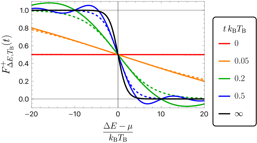
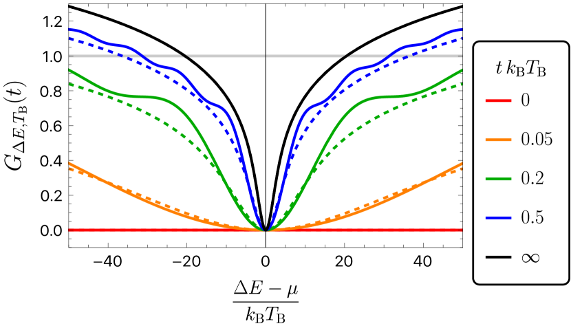
Figure 1: Solid lines show the real part $F^{+}_{\Delta E,T_{\text{B}}}(t)$ (top) and the imaginary part $G_{\Delta E,T_{\text{B}}}(t)$ (bottom) of the coefficients $A^{+}_{m}(t,\Delta E)$ as functions of $\Delta E$ in units of $k_{\text{B}}T$. The dashed lines show the approximations based on the time-dependent temperature $T(t)$, the real part ${\cal F}^{+}_{\Delta E,T_{\text{B}}}(t)$ (top) and the imaginary part ${{\cal G}}_{\Delta E,T_{\text{B}}}(t)$ (bottom). Different colors correspond to various times $t$. For $t=0$ (red) and $t\rightarrow\infty$ (black), the solid and dashed lines match together. The original real parts $F^{+}_{\Delta E,T_{\text{B}}}(t)$ overshoot the interval $[0,1]$ while their approximations stay within it.

Our main finding, from the technical point of view, is that the integral in (17) can be uniformly in $t,\Delta E$ and $T_{\text{B}}$ approximated by the function

$$I =k_{\text{B}}T_{\text{B}}\int_{0}^{t-t_{0}}\frac{\sin[(\Delta E-\mu)\tau]}{\sinh(\pi k_{\text{B}}T_{\text{B}}\tau)}d\tau$$ (20)

$$\approx\frac{1}{\pi}\mbox{Si}\left[\frac{\pi(\Delta E-\mu)}{4k_{\text{B}}T_{\text{B}}}\tanh\left(\frac{4k_{\text{B}}T_{\text{B}}(t-t_{0})}{\pi}\right)\right],$$ (21)

with Si being the sine integral function. It relies on the astonishing similarity (58) discussed in App. C (cf. Fig. 9). It still shows the unwanted excess oscillations as in original $F^{\pm}_{\Delta E,T_{\text{B}}}(t)$ (cf. Fig. 1). These can be most clearly observed in the limit $T_{\text{B}}\rightarrow 0$ when (21) becomes exact

$$I=\int_{0}^{t-t_{0}}\text{d}\tau\frac{\sin[(\Delta E-\mu)\tau]}{\pi\tau}=\frac{\mbox{Si}[(\Delta E-\mu)(t-t_{0})]}{\pi}$$ (22)

and can assume values out of the range $[-\frac{1}{2},\frac{1}{2}]$ which may lead to negative values of $F^{\pm}_{\Delta E,T_{\text{B}}}(t)$ in (17). Therefore, in the last step, we replace the sine integral function by $\tanh$ which has a similar form but stays bounded in the proper region without any oscillations (cf. Fig. 9), by which we arrive at

$$I \approx\frac{1}{2}\tanh\left[\frac{(\Delta E-\mu)}{2\,k_{\text{B}}T_{\text{B}}}\tanh\left(\frac{4\,k_{\text{B}}T_{\text{B}}(t-t_{0})}{\pi}\right)\right]$$ (23)

(cf. App. C.2 for the full derivation).

In the limit $t\rightarrow\infty$ the approximation (23) becomes an equality (with the inner $\tanh(\infty)=1$) and inserted into (17) delivers the static Fermi function (19). By inserting the full approximation obtained in (23) into the formula (17) and denoting the approximated coefficients as ${\cal F}^{\pm}_{\Delta E,T_{\text{B}}}(t)$ we find that the result can be recast as a Fermi function, too, (cf. Fig. 1, top)

$$F^{\pm}_{\Delta E,T_{\text{B}}}(t)\approx{\cal F}^{\pm}_{\Delta E,T_{\text{B}}}(t)\equiv F^{\pm}_{\Delta E,T(t)}(\infty)=f_{\pm}(\Delta E,T(t)),$$ (24)

now with a modified, time–dependent temperature

$$T(t)=T_{\text{B}}\Bigl{/}\tanh\left(\frac{4k_{\text{B}}T_{\text{B}}}{\pi}(t-t_{0})\right),$$ (25)

(cf. Fig. 2).

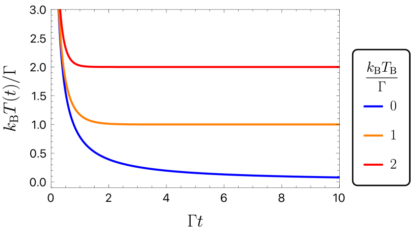
Figure 2: Evolution of the time–dependent effective temperature $T(t)$ for various temperatures of the bath $T_{\text{B}}$.

The effective temperature $T(t)$ is universal, i.e. independent of $\Delta E$. It diverges at short times,

$$T(t)\approx\frac{\pi}{4k_{\text{B}}(t-t_{0})}\equiv T_{0}(t)\quad\text{for}\quad t-t_{0}\ll\frac{1}{k_{\text{B}}T_{\text{B}}}$$ (26)

and converges to the true bath temperature $T(t)\rightarrow T_{\text{B}}$ for late times $t\rightarrow\infty$ (cf. Fig. 2). We will refer to it as the effective contact temperature, for the origin of its time–dependence is in the contact of the system with the environment at $t=t_{0}$ and start of the build–up of correlations (which were assumed to be absent for $t<t_{0}$).

The approximate coefficients directly satisfy three important limiting cases, for $t\rightarrow\infty,t\rightarrow 0$ and $T_{\text{B}}\rightarrow\infty$, which can be directly obtained from the integral (17) and the fourth limiting case, for $T_{\text{B}}\rightarrow 0$, which resolves the problem of excess oscillations observed in (22) and replaces the result with a non–oscillatory function,

$${\cal F}^{\pm}_{\Delta E,T_{\text{B}}}(t\rightarrow\infty) =\frac{1}{2}\mp\frac{1}{2}\tanh\frac{\Delta E-\mu}{2k_{\text{B}}T_{\text{B}}}=f_{\pm}(\Delta E,T_{\text{B}}),$$

$${\cal F}^{\pm}_{\Delta E,T_{\text{B}}}(t\rightarrow 0) =\frac{1}{2}=f_{\pm}(\Delta E,\infty),$$

$${\cal F}^{\pm}_{\Delta E,T_{\text{B}}\rightarrow\infty}(t) =\frac{1}{2}=f_{\pm}(\Delta E,\infty),$$

$${\cal F}^{\pm}_{\Delta E,T_{\text{B}}\rightarrow 0}(t) =\frac{1}{2}\mp\frac{1}{2}\tanh\!\frac{2(\Delta E-\mu)(t-t_{0})}{\pi}$$

$$=f_{\pm}(\Delta E,T_{0}(t)),$$ (27)

where $T_{0}(t)$ is given in (26). In all cases ${\cal F}^{\pm}_{\Delta E,T_{\text{B}}}(t)$ stays in the required range $[0,1]$ (cf. Fig. 1, top).

Approach	Coefficients	Value	for $T_{\text{B}}=0$
Redfield–I	$F^{\pm}_{\Delta E,T_{\text{B}}}(t)$		$\frac{1}{2}\mp\mbox{Si}(\Delta Et)/\pi$
modified Redfield–I	${\cal F}^{\pm}_{\Delta E,T_{\text{B}}}(t)=f_{\pm}(\Delta E,T(t))$	$\frac{1}{2}\mp\frac{1}{2}\tanh\left[\frac{\Delta E}{2\,k_{\text{B}}T_{\text{B}}}\tanh\left(\frac{4\,k_{\text{B}}T_{\text{B}}t}{\pi}\right)\right]$	$\frac{1}{2}\mp\frac{1}{2}\tanh\left(\frac{2\Delta Et}{\pi}\right)$
static Redfield–II	$F^{\pm}_{\Delta E,T_{\text{B}}}(\infty)=f_{\pm}(\Delta E,T_{\text{B}})$	$\frac{1}{2}\mp\frac{1}{2}\tanh\left(\frac{\Delta E}{2\,k_{\text{B}}T_{\text{B}}}\right)$	$\Theta(-\Delta E)$

Table 1: Overview of the discussed approximation schemes. The constants $\mu$ and $t_{0}$ were set to zero for brevity.

IV.2 Imaginary part of $A^{\pm}_{m}(t,\Delta E)$

After we have considered the real part of $A^{\pm}_{m}(t,\Delta E)$ we next focus on its imaginary part. In the wideband limit, $\text{Im}\,A^{\pm}_{m}(t,\Delta E)$ diverges. However, (9) and (14) contain only differences, $\text{Im}\,A^{\pm}_{m}(t,\Delta E)-\text{Im}\,A^{\pm}_{m}(t,\Delta E^{\prime})$, which are finite. Therefore we define

$$\Gamma_{m}G_{\Delta E,T_{\text{B}}}(t)=\mbox{Im}\,A^{\pm}_{m}(t,\Delta E)-\mbox{Im}\,A^{\pm}_{m}(t,\mu)$$ (28)

(which is independent of $\pm$) by choosing a universal value, $\Delta E^{\prime}=\mu$, for the counter–term and obtain

$$G_{\Delta E,T_{\text{B}}}(t)\equiv k_{\text{B}}T_{\text{B}}\int_{0}^{t-t_{0}}\frac{1-\cos[(\Delta E-\mu)\tau]}{\sinh(\pi k_{\text{B}}T_{\text{B}}\tau)}d\tau.$$ (29)

Applying similar approximations as for the real part of $A^{\pm}_{m}(t,\Delta E)$ we find

$$G_{\Delta E,T_{\text{B}}}(t)\approx\frac{1}{\pi}\text{Re}\Biggl{[}\psi\left(\frac{1}{2}+i\frac{\Delta E-\mu}{2\pi k_{\text{B}}T(t)}\right)-\psi\left(\frac{1}{2}\right)\Biggr{]}$$ (30)

with the same effective temperature $T(t)$ as in (25) (cf. Fig. 1 and App. C.3). Denoting the right–hand side by ${\cal G}_{\Delta E,T_{\text{B}}}(t)$, we arrive, in full analogy to (24), at

$$G_{\Delta E,T_{\text{B}}}(t)\approx{\cal G}_{\Delta E,T_{\text{B}}}(t)\equiv G_{\Delta E,T(t)}(\infty).$$ (31)

This confirms that the effective contact temperature $T(t)$ can be used in both, the real and the imaginary part of $A^{\pm}_{m}(t,\Delta E)$.

In the next two sections, V and VI, we will consider a simple system consisting of a single quantum dot in order to compare the different approaches analytically and numerically:

• exact solutions (for the non–interacting system),

• Redfield–I equation with time–dependent coefficients $F^{\pm}_{\Delta E,T_{\text{B}}}(t)$ leading to positivity problem 1 due to overshooting the range $[0,1]$,

• modified Redfield–I equation with approximate coefficients ${\cal F}^{\pm}_{\Delta E,T_{\text{B}}}(t)\in[0,1]$ based on time–dependent temperature $T(t)$,

• Redfield–II equation with static coefficients $F^{\pm}_{\Delta E,T_{\text{B}}}(\infty)\in[0,1],$

summarized in Tab. 1. We will concentrate only on the real part $F^{\pm}_{\Delta E,T_{\text{B}}}(t)$ since the imaginary part $G_{\Delta E,T_{\text{B}}}(t)$ will not be significant for that system. For larger systems than one quantum dot, we would also deal with the problem 2 of non–positivity of some $2\times 2$ matrix valued coefficients, ${\cal M}\ngeq 0$, in which case we might want to further approximate the Redfield–I and II equations to the Lindblad form with modified $\widetilde{\cal M}\geq 0$ (cf. App. A), [45].

V Example: single Quantum dot

Here, we consider a simple system to demonstrate the application of the above proposed approximation method based on the time–dependent temperature. We choose a single quantum dot described by

$$H_{\text{S}}=Un_{\uparrow}n_{\downarrow}+\epsilon(n_{\uparrow}+n_{\downarrow})$$ (32)

with $n_{s}=c^{\dagger}_{s}c_{s}$, spin $s=\uparrow,\,\downarrow$, Coulomb interaction $U>0$ and onsite energy $\varepsilon$, satisfying $-U<\varepsilon-\mu<0$. The system has $\dim(S)=4$ eigenstates, cf. (2), and is connected to $M=2$ baths with different spin polarizations, cf. (3) and (4). Both, in the static (second) Markov approximation, for $t_{0}\rightarrow-\infty$, as well as in the time–dependent effective temperature approximation, with $t_{0}=0$, (12) reduces to a GKSL equation (cf. App. A) with the Lindblad dissipators (54) or (56) (which differ only by non–physical coherences between states with different occupation numbers)

$$L^{\pm}_{s,1} =\sqrt{f_{\pm}(\varepsilon,\widetilde{T}(t))}\,c^{\pm}_{s}(1-n_{\bar{s}}),$$ (33)

$$L^{\pm}_{s,2} =\sqrt{f_{\pm}(\varepsilon+U,\widetilde{T}(t))}\,c^{\pm}_{s}n_{\bar{s}},$$ (34)

for tunneling in/out ($\pm$) of the first (33) and second electron (34) with spin $s$. The temperature $\widetilde{T}(t)$ in the Fermi functions $f_{\pm}$ is either constant and equal $T_{\text{B}}$ or time–dependent as given by (25). In the static case, for $T_{\text{B}}=0$, the states $\Ket{\uparrow}\!\!\Bra{\uparrow}$ and $\Ket{\downarrow}\!\!\Bra{\downarrow}$ are “frozen”. However, the effective time–dependent temperature $T(t)$, even for $T_{\text{B}}=0$, becomes initially large, $T(t\approx 0)\rightarrow\infty$, cf. (26), and the system is temporarily driven towards the fully mixed “hot” state

$$\rho_{\infty}=\frac{1}{4}\Bigl{[}\Ket{0}\!\!\Bra{0}+\Ket{\uparrow}\!\!\Bra{\uparrow}+\Ket{\downarrow}\!\!\Bra{\downarrow}+\Ket{\uparrow\downarrow}\!\!\Bra{\uparrow\downarrow}\Bigr{]}.$$ (35)

Eventually, as $T(t)\rightarrow T_{\text{B}}=0$, it relaxes to some mixture $a\Ket{\uparrow}\!\!\Bra{\uparrow}+b\Ket{\downarrow}\!\!\Bra{\downarrow}$ with $a+b=1$. Starting with the pure state $\Ket{\uparrow}\!\!\Bra{\uparrow}$, the final spin–$z$ $\Braket{S_{z}}=(a-b)/2$ will measure how strong the influence of the “hot” period on the effective dynamics was. This observable satisfies an autonomous differential equation (valid for any $T_{\text{B}}$)

$$\dot{S}^{\text{eff}}_{z}(t)=-\Gamma\bigl{[}1-f_{+}(\epsilon,T(t))+f_{+}(\epsilon+U,T(t))\bigr{]}S^{\text{eff}}_{z}(t)$$ (36)

which can be integrated to

$$S^{\text{eff}}_{z}(t)=S_{z}(0)\exp\left[-2\Gamma\int_{0}^{t}\text{d}t^{\prime}f_{+}(\epsilon+U,T(t^{\prime}))\right]$$ (37)

where we have chosen the special value $\varepsilon=\mu-U/2$ for convenience. For $T_{\text{B}}>0$ this integral is difficult to calculate but it diverges for $t\rightarrow\infty$ and thus leads to $S_{z}(\infty)=0$. For $T_{\text{B}}=0$, we have $k_{\text{B}}T(t)=\pi/(4t)$ (cf. (25)) and this integral can be calculated exactly to give

$$S^{\text{eff}}_{z}(t)=S_{z}(0)\,e^{-2\Gamma t}\left(1+e^{\frac{2U}{\pi}t}\right)^{\frac{\Gamma\pi}{U}}2^{-\pi\frac{\Gamma}{U}}$$ (38)

which for $t\gg 1/U$ has the limit

$$S^{\text{eff}}_{z}(t)\cong 2^{-\pi\Gamma/U}S_{z}(0).$$ (39)

It means that the initial spin–z, $S_{z}(0)$, decays in a non–perturbative way, which is enhanced by the system–bath coupling $\Gamma$ and suppressed by the Coulomb repulsion $U$. This is in contradiction to the observation that both pure states are “frozen” in the static (second) Markov case.

Also for the not approximated Redfield–I master equation (12) the spin–$z$ can be calculated analogously to (37)

$$S_{z}(t)=S_{z}(0)\exp\left[-2\,\Gamma\int_{0}^{t}F^{+}_{\Delta E=\epsilon+U,T_{\text{B}}}(t^{\prime})\,dt^{\prime}\right].$$ (40)

In this particular system and for $T_{\text{B}}=0$ the integral can be evaluated exactly and gives

$$S_{z}(t)=S_{z}(0)\,e^{-\Gamma t}\times\\ \exp\Biggl{[}\frac{4\,\Gamma}{\pi U}\left(\cos\left(\frac{Ut}{2}\right)-1\right)+\frac{2\,\Gamma\,t}{\pi}\mbox{Si}\left(\frac{Ut}{2}\right)\Biggr{]}$$ (41)

which for $t\gg 1/U$ gives

$$S_{z}(t)\cong e^{-4\,\Gamma/(\pi U)}S_{z}(0).$$ (42)

Due to $2^{-\pi\Gamma/U}<e^{-4\,\Gamma/(\pi U)}$, the approximation with the effective temperature (39) slightly overestimates the effect compared to the prediction of the Redfield–I master equation (42), however, both stay within the same order of magnitude which justifies the effective temperature approximation (cf. Fig. 3). On the other hand, the Redfield–I master equation (12) does not preserve the positivity of the density matrix (cf. Sec. IV) and leads to negative probability, as shown in Fig. 3 (second from bottom) whereas the effective temperature approximation is free of this problem. For bath temperatures $T_{\text{B}}>0$, both results decay to $S_{z}(\infty)=0$ at late times. However, at short times, $t\ll\tau_{\text{c}}$, and small bath temperature $T_{\text{B}}$, the Redfield–I master equation and the effective temperature approximation give $S_{z}(t)\sim\exp\left(-\Gamma t\right)$ while in the static approximation the decay is exponentially suppressed, $S_{z}(t)\sim\exp\left(-2\,\Gamma e^{-U/(2k_{\text{B}}T_{\text{B}})}t\right)$.

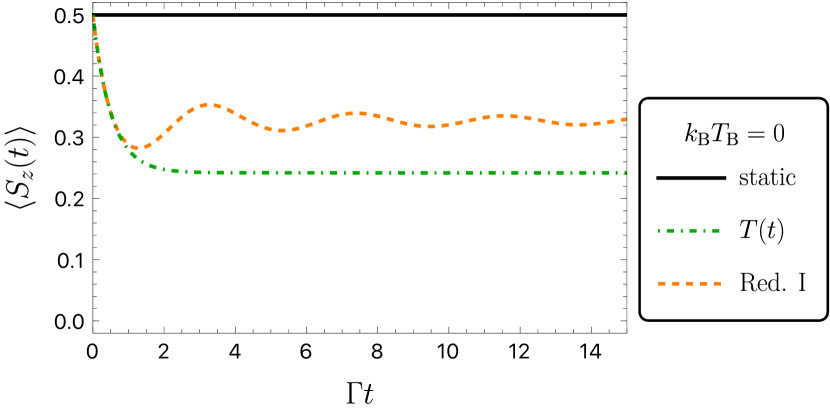
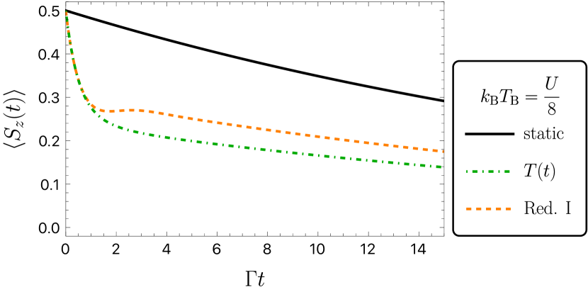
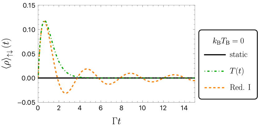
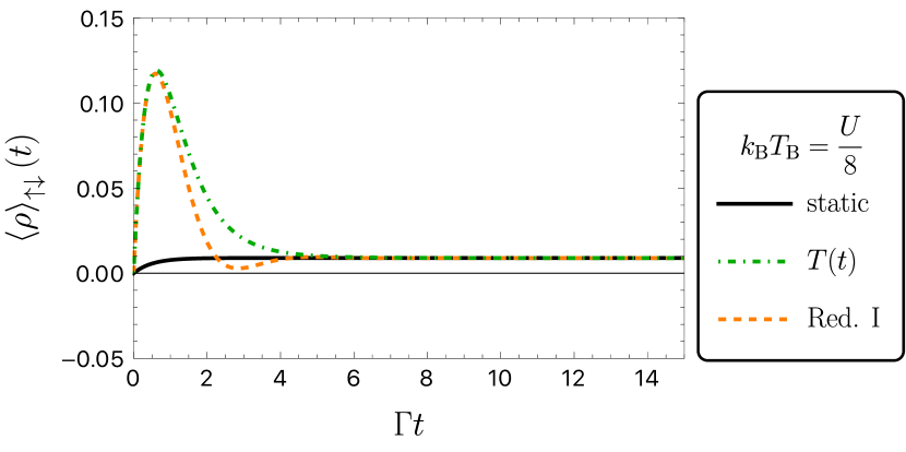
Figure 3: One quantum dot. Top pair: spin $\Braket{S_{z}(t)}$ as a function of time for the static Markov and the effective temperature approximations as well as for the Redfield–I master equation (12). The Coulomb interaction is $U=3\,\Gamma$, the onsite potential is $\epsilon=\mu-\frac{U}{2}$, and the bath temperature is $T_{\text{B}}=0$ or $k_{\text{B}}T_{\text{B}}=U/8$. The initial state is $\rho_{S}(0)=\Ket{\uparrow}\!\!\Bra{\uparrow}$. Bottom pair: Probability of the double occupation $\Braket{\rho}_{\uparrow\downarrow}(t)\equiv\braket{\uparrow\downarrow}{\rho(t)}{\uparrow\downarrow}$ as a function of time, here identical with the zero occupation $\Braket{\rho}_{0}(t)\equiv\braket{0}{\rho(t)}{0}$. Both can get negative for the Redfield equation. The energy, given by $\Braket{H_{\text{S}}-\mu N}=U\left[\Braket{\rho}_{\uparrow\downarrow}+\Braket{\rho}_{0}-1\right]/2$ with $N=n_{\uparrow}+n_{\downarrow}$, also swings below its theoretical lower limit $-U/2$ for $T_{\text{B}}=0$. The parameters are the same as for $\Braket{S_{z}(t)}$, respectively.

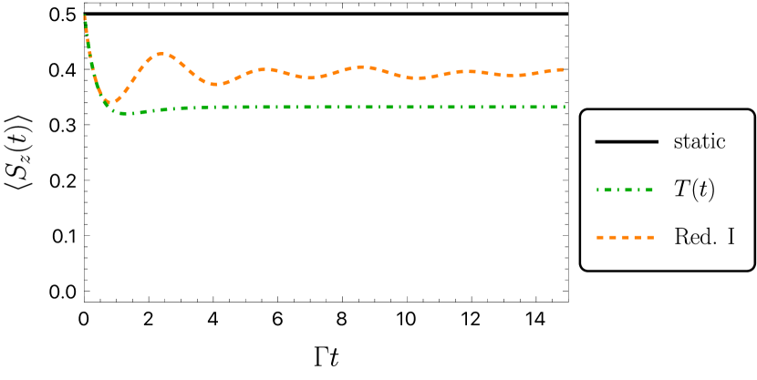
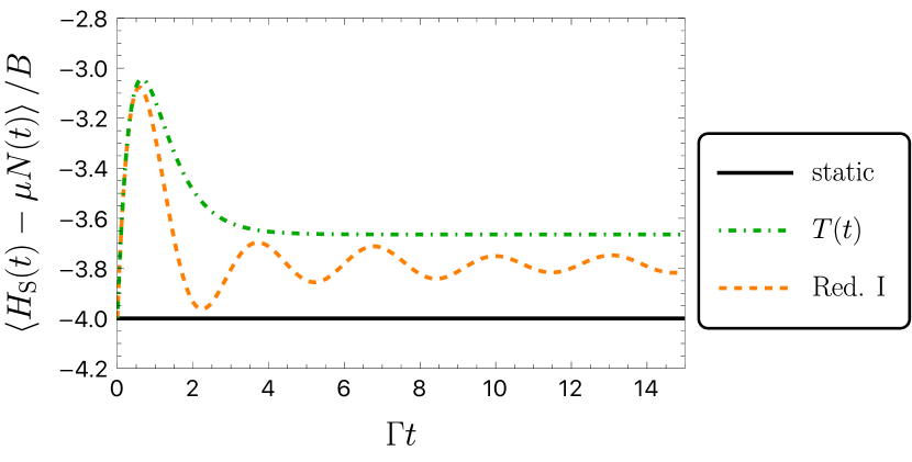
Figure 4: One quantum dot. Spin $\Braket{S_{z}(t)}$ (top) and energy $\Braket{H_{\text{S}}(t)-\mu N(t)}$ with $N=n_{\uparrow}+n_{\downarrow}$ (bottom) as functions of time for the static Markov and the effective temperature approximations as well as for the Redfield–I master equation (12). The Coulomb interaction is $U=3\,\Gamma$, the onsite potential is $\epsilon=\mu-U/2$, the bath temperature is $T_{\text{B}}=0$, the magnetic field is $B=\Gamma/2$, and the initial state is $\rho_{S}(0)=\Ket{\uparrow}\!\!\Bra{\uparrow}$ (ground state).

By a similar mechanism, the contact temperature can even lead to an excitation of the ground state and deposit energy into the system. By adding a magnetic field in the $z$–direction with the Hamiltonian $H_{z}=2BS_{z}$ we obtain together with (32)

$$H_{S}=Un_{\uparrow}n_{\downarrow}+(\varepsilon-B)n_{\uparrow}+(\varepsilon+B)n_{\downarrow}$$ (43)

and lift the degeneracy between the $\ket{\uparrow}$ and $\ket{\downarrow}$ states. We choose $T_{\text{B}}=0$ and start in the ground state $\rho_{S}(0)=\Ket{\uparrow}\!\!\Bra{\uparrow}$. By connecting the system with the bath at $t=t_{0}=0$, due to the high effective temperature $T(t)$ at short times, there will be an increase of energy in the system

$$\Delta H_{\text{S}}=H_{\text{S}}(\infty)-H_{\text{S}}(0)=-2B(S_{z}(\infty)-S_{z}(0)),$$ (44)

cf. Fig. 4. In the limit of weak $B$, it can be evaluated to

$$\Delta H_{\text{S}}=B\left(1-e^{-4\,\Gamma/(\pi U)}\right)+\mathcal{O}\left(\frac{B^{2}}{U}\right)$$ (45)

for the Redfield–I master equation (12) and to

$$\Delta H_{\text{S}}=B\left(1-2^{-\pi\Gamma/U}\right)+\mathcal{O}\left(\frac{B^{2}}{U}\right)$$ (46)

for the effective temperature approximation, where again the latter method slightly overestimates the result.

VI Non–interacting quantum dot as benchmark

Since the proposed effective temperature method is an approximation to the Redfield equation which in turn is also an approximation itself, it does not provide a proper benchmark for testing the accuracy. Especially, in the situations when the Redfield equation leads to mathematical problems the comparison is unclear. Therefore, we consider here the non–interacting case with $U=0$ which is exactly solvable and compare the different master equation approaches with it.

Without the Coulomb interaction, the system splits into two identical copies of a spinless system

$$H=\epsilon\,n+\sum_{k}\left(\gamma_{k}c\,a_{k}^{\dagger}+\text{h.c.}\right)+\sum_{k}\epsilon_{k}a_{k}^{\dagger}a_{k}$$ (47)

with $n=c^{\dagger}c$. Starting from the Heisenberg equation of motion and Laplace transformation technique [8, 10], it is possible to express the annihilation operator of the dot in the Heisenberg picture

$$c_{\text{H}}(t)=e^{-i\epsilon t-\frac{\Gamma}{2}t}c_{\text{H}}(0)+\sum_{k}\gamma_{k}^{*}a_{k}\left(\frac{e^{-i\epsilon t-\frac{\Gamma}{2}t}-e^{-i\epsilon_{k}t}}{i(\epsilon_{k}-\epsilon)-\frac{\Gamma}{2}}\right)$$ (48)

in terms of the operators $c=c_{\text{H}}(0)$ and $a_{k}$ in the Schrödinger picture. Assuming an initial product state between the dot and a Fermi distributed bath leads to

$$\left<n(t)\right>=e^{-\Gamma t}\left<n(0)\right>\\ +\Gamma\int_{-\infty}^{\infty}\frac{\text{d}\omega}{2\pi}f_{+}(\omega+\epsilon,T_{\text{B}})\frac{e^{-\Gamma t}+1-2\cos(\omega t)e^{-\frac{\Gamma}{2}t}}{\omega^{2}+\frac{\Gamma^{2}}{4}}.$$ (49)

Fig. 5 compares the exact solution (49) and the different master equations as functions of time.

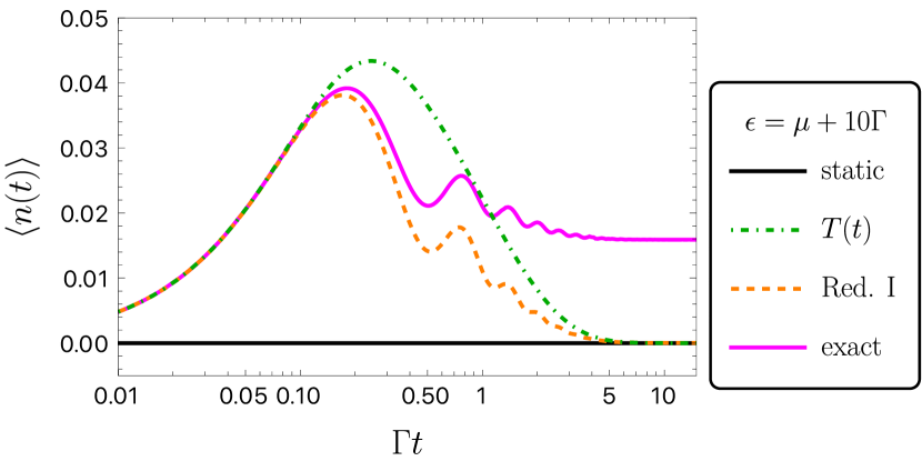
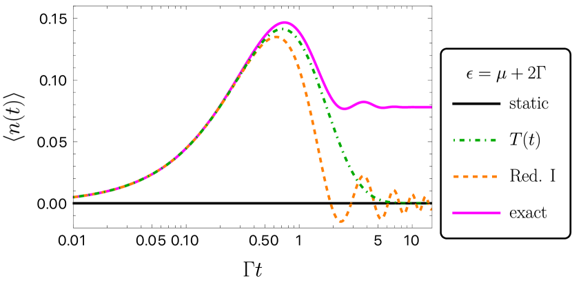
Figure 5: Particle number $\left<n(t)\right>$ as a function of time (logarithmic scale). The lines show the various master equations and exact solution (49) with $T_{\text{B}}=0$, $U=0$, $\Braket{n(0)}=0$ and $\epsilon=\mu+10\,\Gamma$ (top) or $\epsilon=\mu+2\,\Gamma$ (bottom).

Due to forbidden energy transitions for $\epsilon>\mu$ and $T_{\text{B}}=0$, the static approximation leads to no dynamics when starting with an initially empty dot. In contrary, the exact solution and both time–dependent Redfield–I master equations, original and modified with the effective temperature, describe relaxation for short times, $t\lesssim\tau_{\text{c}}$. In this regime, the exact solution agrees with both time–dependent Redfield–I master equations. It justifies the special behavior of the time–dependent effective temperature $T(t)$ at short times which is necessary for the correct description of the dynamics and reflects the physical consequence of the initial connection between the quantum dot and the bath.

For later times $t>\tau_{\text{c}}$ and the chosen parameters, the exact solution deviates from all master equation solutions by the same order of magnitude which can be asymptotically described by $\left|\left<n(\infty)\right>_{\text{exact}}-\left<n(\infty)\right>_{\text{ME}}\right|\approx\Gamma/(2\pi|\epsilon-\mu|)$. It is important to note that the effect of both time–dependent master equations compared to the static Markov approximation decays as $\Gamma/|\epsilon-\mu|$, too.

Summarizing, both time–dependent master equations show a perfect agreement with the exact solution for short times $t\lesssim\tau_{\text{c}}$. This is even true for parameters where $|\epsilon-\mu|$ is small and the master equations may fail for later times.

VII Conclusions

We considered a quantum system connected to a thermal bath at fixed temperature $T_{\text{B}}$. By eliminating the bath from the description we derived an approximation of the first Redfield equation with time–dependent coefficients which offers the interpretation of an effective time–dependent temperature $T(t)$ (25). For times smaller than the characteristic time $\tau_{\text{c}}$ (18), the effective temperature is very large, $T(t)\rightarrow\infty$, which can be explained by the fact that at short timescales all energetically forbidden transitions are allowed. At timescales much larger than $\tau_{\text{c}}$, the effective temperature $T(t)$ converges against the true environment temperature $T_{\text{B}}$. The use of the effective temperature $T(t)$ fixes also the problems of non–positivity in the development of the density matrix by the Redfield equation.

We demonstrated these effects on the example of a single quantum dot with Coulomb interaction (Sec. V) which we also compared with exact solutions for a system without the Coulomb interaction, using it as a benchmark (Sec. VI). In both cases we have shown a qualitative and quantitative agreement between the solutions of the original time–dependent Redfield master equation and its approximation based on the time–dependent temperature. In the case without the Coulomb interaction, we have shown a good agreement between the solutions of the Redfield equations and the exact solution. For short times, we see a perfect agreement even for parameters for which the Redfield approximation generally does not hold at later times. This confirms that the effective temperature scheme offers an approximation which is as close to the exact solution as the original Redfield equation and combines a perfect match at short times with being free of any mathematical flaws at later times.

The time–dependent temperature approximation implicitly accounts for non–Markovian processes in the baths and comprises the formation of coherences between the environment and the system. It lefts open space for further approximations and, therefore, can be applied to various types of originally time–independent master equations, beyond the secular approximation or time–averaging methods.

VIII Acknowledgments

The authors thank Gernot Schaller for fruitful discussions and valuable feedback on the manuscript. We gratefully acknowledge funding by the Deutsche Forschungsgemeinschaft (DFG, German Research Foundation) — Project 278162697 — SFB 1242.

Appendix A From Redfield to Lindblad

In the derivation of the Redfield–I equation (8) (cf. Sec. III), at the lowest order in the system–environment coupling strength, the preservation of positivity of the density matrix in the evolution gets lost. Here, we discuss its corrections leading towards GKSL master equations [33, 34, 35, 25, 32, 1, 27].

For transition processes in the system involving the energy differences, $\Delta E$ and $\Delta E^{\prime}$, we consider the blocks

$$\begin{split}{\cal M}^{\pm}_{\Delta E,\Delta E^{\prime}}(t)&=\begin{pmatrix}M_{\pm}(t,\Delta E,\Delta E),&M_{\pm}(t,\Delta E,\Delta E^{\prime})\\ M_{\pm}(t,\Delta E^{\prime},\Delta E),&M_{\pm}(t,\Delta E^{\prime},\Delta E^{\prime})\end{pmatrix}\\ &=\begin{pmatrix}F^{\pm}_{\Delta E,T_{\text{B}}}(t),&\frac{F^{\pm}_{\Delta E,T_{\text{B}}}(t)+F^{\pm}_{\Delta E^{\prime},T_{\text{B}}}(t)}{2}+i\frac{G_{\Delta E,T_{\text{B}}}(t)-G_{\Delta E^{\prime},T_{\text{B}}}(t)}{2}\\ \frac{F^{\pm}_{\Delta E,T_{\text{B}}}(t)+F^{\pm}_{\Delta E^{\prime},T_{\text{B}}}(t)}{2}-i\frac{G_{\Delta E,T_{\text{B}}}(t)-G_{\Delta E^{\prime},T_{\text{B}}}(t)}{2},&F^{\pm}_{\Delta E^{\prime},T_{\text{B}}}(t)\end{pmatrix}\end{split}$$ (50)

built with $M_{\pm}(t,\Delta E,\Delta E^{\prime})\equiv M_{m}^{\pm}(t,\Delta E,\Delta E^{\prime})/\Gamma_{m}$ independent of $m$ (the coefficients $F$ and $G$ are defined in (17) and (29), respectively). If the coefficients $F^{\pm}_{\Delta E,T_{\text{B}}}(t)$ become negative (cf. Fig. 1) the blocks ${\cal M}$ cease to be positive definite what translates also into the total Liouville operator (13). Therefore, we propose in this work the approximation (24) which replaces them with new coefficients ${\cal F}^{\pm}_{\Delta E,T_{\text{B}}}(t)\in[0,1]$. For consistency, we also replace the $G^{\pm}_{\Delta E,T_{\text{B}}}(t)$ coefficients with ${\cal G}^{\pm}_{\Delta E,T_{\text{B}}}(t)$ according to (31) (cf. Sec. IV).

However, in general, also the approximated matrices $\mathcal{M}^{\pm}_{\Delta E,\Delta E^{\prime}}(t)$ are not positive definite for $\Delta E\neq\Delta E^{\prime}$, having one positive and one negative eigenvalue, what presents another possible reason for the the non-positivity of the total Liouville operator (13).

A.1 Secular approximation

The off–diagonal elements of ${\cal M}^{\pm}_{\Delta E,\Delta E^{\prime}}(t)$ correspond to coherences between states with different energies (in the Liouville space), which oscillate in time. The secular approximation [1, 27] averages out the oscillations and effectively removes the off–diagonal terms by which

$$\mathcal{M}^{\pm,\text{sec}}_{\Delta E,\Delta E^{\prime}}(t)=\begin{pmatrix}{\cal F}^{\pm}_{\Delta E,T_{\text{B}}}(t)&0\\ 0&{\cal F}^{\pm}_{\Delta E^{\prime},T_{\text{B}}}(t)\end{pmatrix}$$ (51)

are obviously positive definite. It is equivalent to the replacement of the coefficients $M^{\pm}_{m,s}$ in (14) with

$$M^{\text{sec}}_{\pm}(t,\Delta E,\Delta E^{\prime})=\delta_{\Delta E,\Delta E^{\prime}}{\cal F}^{\pm}_{\Delta E,T_{\text{B}}}(t).$$ (52)

The Liouville superoperator (13) reduces then to the Lindblad form which preserves positivity.

$$\begin{split}&\widetilde{\cal L}\,\rho=\\ &\sum_{\begin{subarray}{c}m,\alpha\\ \Delta E\end{subarray}}\left[L_{m}^{\alpha}(\Delta E)\,\rho\,L_{m}^{\alpha}(\Delta E){}^{\dagger}-\frac{1}{2}\{L_{m}^{\alpha}(\Delta E){}^{\dagger}L_{m}^{\alpha}(\Delta E),\rho\}\right]\end{split}$$ (53)

with the secular Lindblad jump operators

$$L^{\pm,\text{sec}}_{m}(t,\Delta E)=\sqrt{\Gamma_{m}}\times\\ \sum_{i,j}\delta_{\pm\Delta E,E_{i}-E_{j}}\sqrt{{\cal F}^{+}_{E_{i}-E_{j},T_{\text{B}}}(t)}\,\Ket{E_{i}}\!\!\Bra{E_{i}}c^{\pm}_{m}\Ket{E_{j}}\!\!\Bra{E_{j}}$$ (54)

defined for each energy difference $\Delta E=E_{i}-E_{j}$ appearing in the spectrum of the Hamiltonian $H_{\text{S}}$. The double sum runs over all eigenstates $\ket{E_{l}}$ of the system Hamiltonian $H_{\text{S}}$ with eigenenergies $E_{l}$. As we see, the secular approximation automatically removes the imaginary parts $G_{\Delta E,T_{\text{B}}}(t)$.

A.2 Coherent approximation

Because the secular approximation removes too much information and can miss important physics, we developed in [25, 32], along the lines of [33, 34, 35], the coherent approximation as the least invasive method of restoring positivity. The arithmetic mean of the real parts in the off-diagonal terms of $\mathcal{M}^{\pm}_{\Delta E,\Delta E^{\prime}}(t)$ is replaced by the geometric mean while the imaginary parts are removed

$$\mathcal{M}^{\pm,\text{coh}}_{\Delta E,\Delta E^{\prime}}(t)=\\ \begin{pmatrix}{\cal F}^{\pm}_{\Delta E,T_{\text{B}}}(t),&\sqrt{{\cal F}^{\pm}_{\Delta E,T_{\text{B}}}(t){\cal F}^{\pm}_{\Delta E^{\prime},T_{\text{B}}}(t)}\\ \sqrt{{\cal F}^{\pm}_{\Delta E,T_{\text{B}}}(t){\cal F}^{\pm}_{\Delta E^{\prime},T_{\text{B}}}(t)},&{\cal F}^{\pm}_{\Delta E^{\prime},T_{\text{B}}}(t)\end{pmatrix}.$$ (55)

In this way, the negative eigenvalue gets shifted up to zero while the diagonal elements, directly influencing energy populations, stay untouched. The Liouville operator (53) is then given in terms of the coherent Lindblad jump operators

$$L^{\pm,\text{coh}}_{m}(t)=\\ \sqrt{\Gamma_{m}}\sum_{i,j}\sqrt{{\cal F}^{\pm}_{E_{i}-E_{j},T_{\text{B}}}(t)}\,\Ket{E_{i}}\!\!\Bra{E_{i}}c^{\pm}_{m}\Ket{E_{j}}\!\!\Bra{E_{j}}.$$ (56)

They are equal to coherent sums of the secular jump operators, $L^{\pm,\text{coh}}_{m}(t)=\sum_{\Delta E}L^{\pm,\text{sec}}_{m}(t,\Delta E)$ over the spectrum of the energy differences which motivates their name. For more details regarding their derivation and discussion of their properties we refer to [32, App. A]. Within this approximations, the imaginary parts $G^{\pm}_{\Delta E,T_{\text{B}}}(t)$ are also eliminated.

Appendix B Beyond the wideband limit

In the wideband limit, where $\Gamma(\omega)$ is assumed constant everywhere, we find for the coupling coefficients the finite short–time limit $\lim_{t\rightarrow t_{0}}A_{m}^{\pm}(t,\Delta E)=\Gamma_{m}/2$. For any integrable function $\Gamma(\omega)$, however, the coefficients must vanish at short times $\lim_{t\rightarrow t_{0}}A_{m}^{\pm}(t,\Delta E)=0$ since $|A_{m}^{\pm}(t,\Delta E)|\leavevmode\nobreak\ \leq\leavevmode\nobreak\ \|\Gamma_{m}\|_{1}(t-t_{0})/\pi$ with $\|\Gamma_{m}\|_{1}$ the $L^{1}$–norm. Consequently, the equations (16)–(17) and (28)–(29) cannot hold for very short times, $t-t_{0}\lesssim 1/\|\Gamma_{m}\|_{1}$. In the particular example of a Lorentz–like distribution

$$\Gamma_{m}(\omega) =\frac{\Gamma_{m}\Delta_{\Gamma}^{2}}{\Delta_{\Gamma}^{2}+(\Delta E-\omega)^{2}}, \|\Gamma_{m}\|_{1} =\pi\,\Gamma_{m}\Delta_{\Gamma}$$ (57)

the width $\Delta_{\Gamma}$ determines the scale of agreement with the wideband limit, namely, for $t-t_{0}\!\gg\!1/\Delta_{\Gamma}$ the coefficients $A_{m}^{\pm}(t,\Delta E)$ become well approximated by the wideband limit (cf. Figure 6). (For more general $\Gamma_{m}(\omega)$, the conditions hold analogously with $\Delta_{\Gamma}$ determined by the variation of $\Gamma(\omega)$ [26, Sec. 4].) If additionally $\Delta_{\Gamma}\gg 1/\tau_{\text{c}}=\max\left(k_{\text{B}}T_{\text{B}},|\Delta E-\mu|\right)\gtrsim\Gamma_{m}$ the effects of the time–dependent temperature $T(t)$ become relevant.

Figure 6: Coefficients $F^{\alpha}_{\Delta E,T_{\text{B}}}(t)$ with $\alpha=-$ (solid lines) and $\alpha=+$ (dashed lines) as functions of time. The black lines show $F^{\alpha}_{\Delta E,T_{\text{B}}}(t)$ in the wideband limit (cf. (17)) while other lines show $F^{\alpha}_{\Delta E,T_{\text{B}}}(t)$ for the Lorentzian (57) with $\Delta_{\Gamma}=2(\Delta E-\mu)=2/\tau_{\text{c}}$ (orange) or $\Delta_{\Gamma}=10(\Delta E-\mu)=10/\tau_{\text{c}}$ (blue). The temperature is $T_{\text{B}}=0$ and $\Delta E-\mu>0$.

Appendix C Derivation of the $T(t)$ approximation

In order to derive the approximation (23) we first need to introduce a useful similarity.

C.1 Functional similarity

There holds an astonishing similarity between the two hyperbolic functions

$$\frac{x}{\sinh(x)}\approx\frac{1}{\cosh^{2}(4x/\pi^{2})},$$ (58)

as shown in Fig. 9. Despite intensive (re)search and discussion [47] we did not succeed in providing any elementary proof of it. The constant $4/\pi^{2}$ is chosen by the requirement that both functions have equal integrals over $[0,\infty)$ which will have a physical significance in our applications.

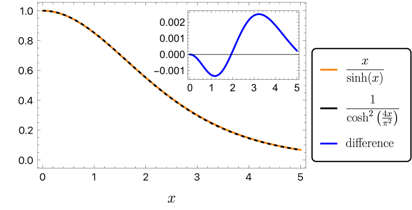
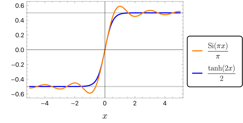
Figure 7: Astonishing similarity between $x/\sinh(x)$ (orange) and $1/\cosh^{2}(4x/\pi^{2})$ (black) with their difference in the inset (blue).

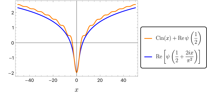
Figure 8: Comparison of ${\mbox{Si}(\pi x)}/{\pi}$ (orange) with ${\tanh(2x)}/{2}$ (blue) as functions of $x$.

Figure 9: Comparison of $\text{Cin}(x)+\text{Re}\left[\psi(1/2)\right]$ (orange) with $\text{Re}\left[\psi\left(1/2+2ix/\pi^{2}\right)\right]$ (blue) as functions of $x$.

C.2 Estimation of the integral (20)

Here, we will apply the discovered functional similarity (58) to the integral (20). First we split the integrand into a product and use the similarity (58) to obtain

$$I =T_{\text{B}}\int_{0}^{t-t_{0}}\frac{\sin(\Delta E^{\prime}\tau)}{\sinh(\pi T_{\text{B}}\tau)}d\tau$$ (59)

$$=\frac{\Delta E^{\prime}}{\pi}\int_{0}^{t-t_{0}}\frac{\pi T_{\text{B}}\tau}{\sinh(\pi T_{\text{B}}\tau)}\frac{\sin(\Delta E^{\prime}\tau)}{\Delta E^{\prime}\tau}d\tau$$

$$\approx\frac{\Delta E^{\prime}}{\pi}\int_{0}^{t-t_{0}}\frac{\pi T_{\text{B}}\tau}{\cosh^{2}(4T_{\text{B}}\tau/\pi)}\frac{\sin(\Delta E^{\prime}\tau)}{\Delta E^{\prime}\tau}d\tau$$ (60)

with $\Delta E^{\prime}\equiv\Delta E-\mu$ and omit the Boltzmann constant for shorter notation. In order to calculate this integral analytically, we use in the second factor the following trick: We observe that the first factor contributes significantly only for $4T_{\text{B}}\tau/\pi\lesssim 1$ (and is negligible otherwise) where the $\tanh$–function is almost linear so that we can replace $\tau\approx\pi\tanh(4T_{\text{B}}\tau/\pi)/(4T_{\text{B}})$. This brings us to

$$I\approx\frac{\Delta E^{\prime}}{\pi}\int_{0}^{t-t_{0}}\frac{1}{\cosh^{2}\left(\frac{4T_{\text{B}}\tau}{\pi}\right)}\frac{\sin\left(\frac{\pi\Delta E^{\prime}}{4T_{\text{B}}}\tanh\left(\frac{4T_{\text{B}}\tau}{\pi}\right)\right)}{\frac{\pi\Delta E^{\prime}}{4T_{\text{B}}}\tanh\left(\frac{4T_{\text{B}}\tau}{\pi}\right)}d\tau$$ (61)

which, by substituting $u=\frac{\pi\Delta E^{\prime}}{4T_{\text{B}}}\tanh\left(\frac{4T_{\text{B}}\tau}{\pi}\right)$, leads to the result

$$I\approx\frac{1}{\pi}\mbox{Si}\left[\frac{\pi\Delta E^{\prime}}{4T_{\text{B}}}\tanh\left(\frac{4T_{\text{B}}(t-t_{0})}{\pi}\right)\right],$$ (62)

with Si being the sine integral function. The result inherits, however, the disadvantage of the exact coefficient $F_{\Delta E,T_{\text{B}}}(t)$ which overshoots beyond the allowed range, namely, $|I|$ increases above the value $1/2$ which leads to problems (cf. Sec. IV). But its behavior at early and late times $t$ as well as small and large $\Delta E$ values is the same as in the tanh-formula (23) which is free of that problem. Treating the excess oscillations (cf. Fig. 10) as an error of the first order approximation (in the coupling between the system and the bath) we want to correct it to physically acceptable range bearing physical interpretation. For this sake we observe that the sine integral (Si) function is close to $\mbox{Si}(\pi x)/\pi\approx\tanh(2x)/2$ which builds the Fermi function and stays in the proper range (cf. Fig. 9). That replacement delivers the final approximation

$$I\approx\frac{1}{2}\tanh\left[\frac{\Delta E^{\prime}}{2T_{\text{B}}}\tanh\left(\frac{4T_{\text{B}}(t-t_{0})}{\pi}\right)\right]$$ (63)

which, technically, presents our main result (23). The connection to the Fermi function is an essential point which allows us to interpret the final result, used in $F^{\pm}_{\Delta E,T_{\text{B}}}(t)$ (17), as the Fermi distribution with modified, time–dependent temperature $T(t)$ (25).

An alternative way to motivate this approximation [48, Ch. 3] (much simpler to derive but not uniform in $\Delta E$) is to introduce the effective temperature by matching the slopes of the Fermi distribution and of the coefficient $F^{-}_{\Delta E,T_{\text{B}}}(t)$ at $\Delta E=\mu$

$$\begin{split}\frac{1}{4T(t)}&=\left.\frac{\partial F^{-}_{\Delta E,T_{\text{B}}}(t)}{\partial\Delta E}\right|_{\Delta E=\mu}=\int_{0}^{t-t_{0}}\frac{T_{\text{B}}\tau\;d\tau}{\sinh(\pi T_{\text{B}}\tau)}.\end{split}$$ (64)

Using again the astonishing similarity $x/\sinh(x)\approx 1/\cosh^{2}(4x/\pi^{2})$ (cf. (58) in App. C.1 ), (25) follows.

Figure 10: Compared are the exact value of the integral $I$ (59) (orange), Si–tanh approximation (62) (blue) and tanh–tanh approximation (63) (green). The temperature of the bath is $T_{\text{B}}=0.08|\Delta E-\mu|$.

C.3 Estimation of the integral (29)

Applying the same approximations as discussed in Sec. C.2 to the integral (29), we derive

$$G_{\Delta E,T_{\text{B}}}(t)=T_{\text{B}}\int_{0}^{t-t_{0}}\frac{1-\cos(\Delta E^{\prime}\tau)}{\sinh(\pi T_{\text{B}}\tau)}d\tau$$

$$\approx\frac{\Delta E^{\prime}}{\pi}\int_{0}^{t-t_{0}}\frac{\pi T_{\text{B}}\tau}{\cosh^{2}(4T_{\text{B}}\tau/\pi)}\frac{1-\cos(\Delta E^{\prime}\tau)}{\Delta E^{\prime}\tau}d\tau$$

$$\approx\frac{\Delta E^{\prime}}{\pi}\int_{0}^{t-t_{0}}\frac{1}{\cosh^{2}\left(\frac{4T_{\text{B}}\tau}{\pi}\right)}\frac{1-\cos\left(\frac{\pi\Delta E^{\prime}}{4T_{\text{B}}}\tanh\left(\frac{4T_{\text{B}}\tau}{\pi}\right)\right)}{\frac{\pi\Delta E^{\prime}}{4T_{\text{B}}}\tanh\left(\frac{4T_{\text{B}}\tau}{\pi}\right)}d\tau$$

$$=\frac{1}{\pi}\text{Cin}\left[\frac{\pi\Delta E^{\prime}}{4T_{\text{B}}}\tanh\left(\frac{4T_{\text{B}}(t-t_{0})}{\pi}\right)\right]$$ (65)

with $\Delta E^{\prime}\equiv\Delta E-\mu$ and omitting the Boltzmann constant for shorter notation. The cosine integral function is defined by

$$\text{Cin}(x)=\int_{0}^{x}\frac{1-\cos(t)}{t}\text{d}t$$ (66)

and is close to $\text{Cin}(x)\approx\text{Re}\left[\psi\left(1/2+2ix/\pi^{2}\right)-\psi(1/2)\right]$ (cf. Figure 9) where $\psi$ is the digamma function which builds $G_{\Delta E,T_{\text{B}}}(\infty)$ [48, Ch. 3]. Using this replacement, we end up with the approximation

$$G_{\Delta E,T_{\text{B}}}(t)\approx\\ \frac{1}{\pi}\text{Re}\Biggl{[}\psi\left(\frac{1}{2}+i\frac{\Delta E^{\prime}}{2\pi T_{\text{B}}}\tanh\left(\frac{4T_{\text{B}}(t-t_{0})}{\pi}\right)\right)-\psi\left(\frac{1}{2}\right)\Biggr{]}$$ (67)

which is identical to (31).

References

- Breuer and Petruccione [2002] H.-P. Breuer and F. Petruccione, The Theory of Open Quantum Systems (Oxford University Press, 2002).
- Meir and Wingreen [1992] Y. Meir and N. S. Wingreen, Landauer formula for the current through an interacting electron region, Physical Review Letters 68, 2512 (1992).
- Jauho et al. [1994] A.-P. Jauho, N. S. Wingreen, and Y. Meir, Time-dependent transport in interacting and noninteracting resonant-tunneling systems, Phys. Rev. B 50, 5528 (1994).
- Karrlein and Grabert [1997] R. Karrlein and H. Grabert, Exact time evolution and master equations for the damped harmonic oscillator, Physical Review E 55, 153 (1997).
- Stefanucci [2007] G. Stefanucci, Bound states in ab initio approaches to quantum transport: A time-dependent formulation, Phys. Rev. B 75, 195115 (2007).
- Zedler et al. [2009] P. Zedler, G. Schaller, G. Kiesslich, C. Emary, and T. Brandes, Weak-coupling approximations in non-Markovian transport, Phys. Rev. B 80, 045309 (2009).
- Zhang et al. [2012] W.-M. Zhang, P.-Y. Lo, H.-N. Xiong, M. W.-Y. Tu, and F. Nori, General Non-Markovian Dynamics of Open Quantum Systems, Phys. Rev. Lett. 109, 170402 (2012).
- Topp et al. [2015] G. E. Topp, T. Brandes, and G. Schaller, Steady-state thermodynamics of non-interacting transport beyond weak coupling, Europhysics Letters 110, 67003 (2015).
- Ali and Zhang [2017] M. M. Ali and W.-M. Zhang, Nonequilibrium transient dynamics of photon statistics, Phys. Rev. A 95, 033830 (2017).
- Jussiau et al. [2019] E. Jussiau, M. Hasegawa, and R. S. Whitney, Signature of the transition to a bound state in thermoelectric quantum transport, Phys. Rev. B 100, 115411 (2019).
- Jussiau and Whitney [2020] É. Jussiau and R. S. Whitney, Multiple perfectly transmitting states of a single level at strong coupling, Europhysics Letters 129, 47001 (2020).
- Kolovsky [2020] A. R. Kolovsky, Open Fermi-Hubbard model: Landauer’s versus master equation approaches, Phys. Rev. B 102, 174310 (2020).
- Nakagawa et al. [2021] M. Nakagawa, N. Kawakami, and M. Ueda, Exact Liouvillian spectrum of a one-dimensional dissipative Hubbard model, Phys. Rev. Lett. 126, 110404 (2021).
- Queisser and Schützhold [2019] F. Queisser and R. Schützhold, Environment-induced prerelaxation in the Mott-Hubbard model, Phys. Rev. B 99, 155110 (2019).
- Nakajima [1958] S. Nakajima, On quantum theory of transport phenomena: steady diffusion, Progress of Theoretical Physics 20, 948 (1958).
- Zwanzig [1960] R. Zwanzig, Ensemble method in the theory of irreversibility, The Journal of Chemical Physics 33, 1338 (1960).
- König et al. [1996a] J. König, J. Schmid, H. Schoeller, and G. Schön, Resonant tunneling through ultrasmall quantum dots: Zero-bias anomalies, magnetic-field dependence, and boson-assisted transport, Phys. Rev. B 54, 16820 (1996a).
- König et al. [1996b] J. König, H. Schoeller, and G. Schön, Zero-Bias Anomalies and Boson-Assisted Tunneling Through Quantum Dots, Phys. Rev. Lett. 76, 1715 (1996b).
- Timm [2008] C. Timm, Tunneling through molecules and quantum dots: Master-equation approaches, Phys. Rev. B 77, 195416 (2008).
- Redfield [1957] A. G. Redfield, On the theory of relaxation processes, IBM Journal of Research and Development 1, 19 (1957).
- Hartmann and Strunz [2020] R. Hartmann and W. T. Strunz, Accuracy assessment of perturbative master equations: Embracing nonpositivity, Phys. Rev. A 101, 012103 (2020).
- Dümcke and Spohn [1979] R. Dümcke and H. Spohn, The proper form of the generator in the weak coupling limit, Zeitschrift für Physik B Condensed Matter 34, 419 (1979).
- Suárez et al. [1992] A. Suárez, R. Silbey, and I. Oppenheim, Memory effects in the relaxation of quantum open systems, The Journal of chemical physics 97, 5101 (1992).
- Gaspard and Nagaoka [1999] P. Gaspard and M. Nagaoka, Slippage of initial conditions for the redfield master equation, The Journal of chemical physics 111, 5668 (1999).
- Kleinherbers et al. [2020] E. Kleinherbers, N. Szpak, J. König, and R. Schützhold, Relaxation dynamics in a Hubbard dimer coupled to fermionic baths: Phenomenological description and its microscopic foundation, Phys. Rev. B 101, 125131 (2020).
- Litzba [2022] L. Litzba, Relaxationsdynamik in Quantenpunktsystemen: Beschreibung durch zeitabhängige Lindblad-Operatoren und die Rolle von Kopplungsasymmetrie, Master’s thesis, University Duisburg-Essen (2022).
- Davies [1974] E. B. Davies, Markovian master equations, Commun. Math. Phys. 39, 91 (1974).
- Lindblad [1976] G. Lindblad, On the generators of quantum dynamical semigroups, Communications in Mathematical Physics 48, 119 (1976).
- Gorini et al. [1976] V. Gorini, A. Kossakowski, and E. C. G. Sudarshan, Completely positive dynamical semigroups of n-level systems, Journal of Mathematical Physics 17, 821 (1976).
- Chruściński and Pascazio [2017] D. Chruściński and S. Pascazio, A brief history of the gkls equation, Open Systems & Information Dynamics 24, 1740001 (2017).
- Kleinherbers et al. [2021] E. Kleinherbers, P. Stegmann, and J. König, Synchronized coherent charge oscillations in coupled double quantum dots, Phys. Rev. B 104, 165304 (2021).
- Szpak et al. [2023] N. Szpak, G. Schaller, R. Schützhold, and J. König, Relaxation to persistent currents in a Hubbard trimer coupled to fermionic baths (2023), arXiv:2311.06331.
- Kiršanskas et al. [2018] G. Kiršanskas, M. Franckié, and A. Wacker, Phenomenological position and energy resolving Lindblad approach to quantum kinetics, Phys. Rev. B 97, 035432 (2018).
- Davidović [2020] D. Davidović, Completely Positive, Simple, and Possibly Highly Accurate Approximation of the Redfield Equation, Quantum 4, 326 (2020).
- Nathan and Rudner [2020] F. Nathan and M. S. Rudner, Universal Lindblad equation for open quantum systems, Phys. Rev. B 102, 115109 (2020).
- Potts et al. [2021] P. P. Potts, A. A. S. Kalaee, and A. Wacker, A thermodynamically consistent Markovian master equation beyond the secular approximation, New Journal of Physics 23, 123013 (2021).
- D’Abbruzzo et al. [2023] A. D’Abbruzzo, V. Cavina, and V. Goivannetti, A time-dependent regularization of the redfield equation, SciPost Physics 15, 117 (2023).
- Becker et al. [2021] T. Becker, L.-N. Wu, and A. Eckardt, Lindbladian approximation beyond ultraweak coupling, Phys. Rev. E 104, 014110 (2021).
- Trushechkin [2021] A. Trushechkin, Unified Gorini-Kossakowski-Lindblad-Sudarshan quantum master equation beyond the secular approximation, Phys. Rev. A 103, 062226 (2021).
- Whitney [2008] R. S. Whitney, Staying positive: going beyond Lindblad with perturbative master equations, J. Phys. A: Math. Theor. 41, 175304 (2008).
- Schaller et al. [2009] G. Schaller, P. Zedler, and T. Brandes, Systematic perturbation theory for dynamical coarse-graining, Phys. Rev. A 79, 032110 (2009).
- Dann et al. [2022] R. Dann, N. Megier, and R. Kosloff, Non-Markovian dynamics under time-translation symmetry, Phys. Rev. Res. 4, 043075 (2022).
- Nestmann et al. [2021] K. Nestmann, V. Bruch, and M. R. Wegewijs, How Quantum Evolution with Memory is Generated in a Time-Local Way, Phys. Rev. X 11, 021041 (2021).
- Schaller [2014] G. Schaller, Open quantum systems far from equilibrium, Vol. 881 (Springer, 2014).
- Litzba et al. [2024] L. Litzba, N. Szpak, and J. König, Relaxation dynamics in a Hubbard dimer coupled to fermionic baths: time-dependent coherent Lindblad operators and the role of coupling asymmetry (2024), in preparation.
- Nestmann and Wegewijs [2022] K. Nestmann and M. R. Wegewijs, Renormalization group for open quantum systems using environment temperature as flow parameter, SciPost Phys. 12, 121 (2022).
- Szpak [2021] N. Szpak, Astonishing similarity of and , Mathematics Stack Exchange (2021).
- Kleinherbers [2022] E. Kleinherbers, Real-time analysis of single-electron transport through quantum dots, Ph.D. thesis, University Duisburg-Essen (2022).