Distinguishing Neighborhood Representations
Through Reverse Process of GNNs for Heterophilic Graphs

Abstract

Graph Neural Network (GNN) resembles the diffusion process, leading to the over-smoothing of learned representations when stacking many layers. Hence, the reverse process of message passing can sharpen the node representations by inverting the forward message propagation. The sharpened representations can help us to better distinguish neighboring nodes with different labels, such as in heterophilic graphs. In this work, we apply the design principle of the reverse process to the three variants of the GNNs. Through the experiments on heterophilic graph data, where adjacent nodes need to have different representations for successful classification, we show that the reverse process significantly improves the prediction performance in many cases. Additional analysis reveals that the reverse mechanism can mitigate the over-smoothing over hundreds of layers.

1 Introduction

Graph neural networks (GNN) have emerged as an important tool for learning relational data. Earlier attempts aim to learn the node representations from graphs based on a message-passing mechanism. The message-passing neural network framework shows partial success with the homophilic graphs, where the nodes with the same labels are likely to be connected. When the heterophilic graphs, where node labels significantly differ from those of their neighbors, are considered, the models based on the homophilic assumption often perform worse than the naive neural network architectures without considering the relationship between nodes (Zhu et al., 2020).

Two classes of GNNs have been proposed to overcome the limitation on heterophilic graphs. The first class aims to aggregate the information selectively from the neighbors (Chien et al., 2020; Li et al., 2022). For example, aggregating relevant information from multi-hop neighbors or relevant features from neighbors has been proposed in this direction (Zhu et al., 2020; Liang et al., 2023). On the other hand, the other class of methods highlights the importance of initial node features before aggregation. Adding skip-connection to the initial node features or isolating the original node features for prediction has been proposed in this direction (Zhu et al., 2020; Song et al., 2023).

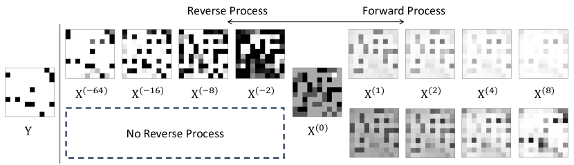
Figure 1: Visualized node representations over the forward and reverse processes in Minesweeper. Top: our approach with the forward and reverse processes. Bottom: a classical GCN with a forward process only. The original node features are smoothed over the forward process, whereas the features are sharpened over the reverse process. Visualization details are provided in Section 4.1.3.

Aggregation is a fundamental mechanism of all GNN models, and heterophilic GNNs are no exception. With a very clever technique, one can mitigate the propagation of irrelevant information for the first few layers. However, GRAND (Chamberlain et al., 2021) shows that GNN can be seen as a discretization of a heat diffusion equation. The diffusion perspective implies that the node representations will eventually reach the stationary state, with which the nodes cannot be distinguished. Therefore, if we cannot isolate all irrelevant nodes in the aggregation process, which is typically impossible, the GNN will eventually aggregate information from irrelevant nodes as the model propagates over and over.

In this work, we claim not to forcefully correct the diffusive nature of the GNNs. Instead, we propose to use the reverse process of the aggregation. The aggregation process is known to smooth the node representations; hence, its reverse process can sharpen the node representations and make the neighborhood representations more distinguishable. To illustrate our intuition, we showcase our experimental results on the Minesweeper dataset, a well-known heterophilic dataset, in Figure 1. In Minesweeper, a board is a grid-structured graph where each node is initialized with the number of mines in the adjacent nodes $\mathbf{X}^{(0)}$, and the goal is to classify the location of mine $\mathbf{Y}$ correctly. The bottom row visualizes the learned node representations with the GCN (Kipf & Welling, 2017), and the top row visualizes the representations with our approach. With the forward-only method, such as GCN, the learned representations cannot be sharpened enough to distinguish the target nodes from the others, whereas when the reverse process is applied to the initial features, we can obtain a sharpened representation from the backward process.

To this end, we propose the framework of reverse process GNNs utilizing the inversion of forward message-passing layers. Specifically, we provide three variants of reverse process GNN based on three backbone models: 1) GRAND (Chamberlain et al., 2021), 2) GCN (Kipf & Welling, 2017), and 3) GAT (Veličković et al., 2018). For GRAND, we directly use the numerical method to obtain the representations in a backward direction. For GCN and GAT, we adopt the idea of iResNet (Behrmann et al., 2019) to make invertible message-passing layers that can model the reverse process.

The experimental results on heterophilic datasets show that the reverse process improves the prediction performance compared with the forward-only models. Our approach produces sharper representations and successfully stacks deep layers to capture long-range dependencies, which are crucial for performance on heterophilic datasets. The experiments on homophilic datasets confirm that the reverse process does not harm the prediction performance when the aggregation mechanism is sufficient. Our investigation reveals that with the reverse process, one can stack hundreds, even a thousand layers, without suffering over-smoothing. Additional experiments with the low-rate label datasets confirm that the reverse process design is effective for tasks where the long-range interaction between nodes is inevitable.

2 Related Work

Most studies on heterophilic data focus on identifying nodes with similar characteristics even among non-adjacent ones for aggregation. GPR-GNN (Chien et al., 2020) utilizes a trainable generalized PageRank for feature aggregation, learning important neighborhood ranges from the data and emphasizing information within those ranges for aggregation. CPGNN (Zhu et al., 2021) introduces a learnable compatibility matrix to capture the information of non-adjacent homophilic nodes. FAGCN (Bo et al., 2021) introduces a GNN framework with a self-gating mechanism to adaptively use low-frequency and high-frequency signals. FSGNN (Maurya et al., 2022) proposes soft feature selection, wherein it adaptively selects node features with different properties. GloGNN (Li et al., 2022) employs a coefficient matrix that represents node-to-node relationships for aggregation, allowing the aggregation of information from all nodes. GBK-GNN (Du et al., 2022) proposes a bi-kernel graph neural network that separately handles homophilic and heterophilic nodes. It uses a selection gate to predict whether a node is homophilic or heterophilic and obtains features using the corresponding kernel based on the prediction. LRGNN (Liang et al., 2023) uses a low-rank approximation to compute a label relationship matrix, employing it for signed message passing.

However, aggregation still causes global node representations to become similar, known as over-smoothing, leading to performance degradation on heterophilic datasets. To overcome this issue, H₂GCN (Zhu et al., 2020) and OGNN (Song et al., 2023) proposes to preserve non-aggregated representation separately. H₂GCN learns node representation by separating ego-embedding and neighbor-embedding and employing intermediate representations. OGNN proposes ordering message passing to prevent the mixing of messages from different hops.

On the other hand, several studies tackle the over-smoothing issue. GRAND (Chamberlain et al., 2021) enhances the understanding of over-smoothing from the perspective of the resemblance between GNN structures and the heat diffusion equation. PairNorm (Zhao & Akoglu, 2020) proposes a normalization layer that remains the total pairwise feature distances constant. DropEdge (Rong et al., 2020) randomly removes edges from the graph to cut off messages passing between adjacent nodes. Half-Hop (Azabou et al., 2023) up-sample edges and slow down the message passing. While delaying or limiting over-smoothing can make node representations less smooth, learning difference-enhanced representations between adjacent nodes, which is helpful for heterophilic data, is still challenging.

3 Method

We aim to introduce a framework that can learn distinct node representations between adjacent nodes through reverse diffusion. We first provide the overall framework of our approach and then show three substantiations of the framework for three baseline models.

3.1 Framework

We consider a graph $\mathcal{G}=(\mathcal{V},\mathcal{E})$, where $\mathcal{V}$ and $\mathcal{E}$ are a set of nodes and edges respectively, with additional $d$-dimensional node features represented as $\mathbf{X}\in\mathbb{R}^{|\mathcal{V}|\times d}$ for all node, and $\mathbf{x}_{i}\in\mathbb{R}^{d}$ denotes the feature of node $i$. It is a well-known fact that a typical GNN layer $f$ tends to learn similar representations between neighboring nodes, leading to the issue of over-smoothing. Chamberlain et al. (2021) highlighted that this is due to the diffusive property inherent in GNN structures.

In contrast to a typical GNN layer, we propose a GNN layer $g$ that performs the opposite role by reversing diffusion and re-concentrating diffused information. Our main idea is to design an inverse function of a message-passing GNN layer $f$, and $g=f^{-1}$ to perform the reversion. Due to the diffusive nature of the GNN layer $f$, its inverse form $g$ is expected to have two properties: 1) $g$ cancels the smoothing effect, producing sharper representations and thus leading to 2) stacking multiple layers of $g$ that do not suffer from the over-smoothing issue.

Formally, with the inverse of multiple message passing layers, our framework predicts node label $\mathbf{Y}$ as follows:

$$\hat{\mathbf{Y}}=\phi(f^{(L)}\circ\cdots\circ f^{(1)}(\mathbf{X}^{(0)})\|g^{(1)}\circ\cdots\circ g^{(L)}(\mathbf{X}^{(0)})),$$

where $\mathbf{X}^{(0)}$ is input node features, $f^{(\ell)}$ is the $\ell$-th forward message-passing layer with $g^{(\ell)}=f^{(\ell)^{-1}}$, $\|$ denotes concatenation, and $\phi$ is a prediction function based on the forward and reverse processes of the input features. We concatenate the representations from both directions for prediction to utilize advantage of difference enhanced representation and smooth representaiton at the same time. In practice, we can set the numbers of forward and reverse steps differently and share the parameters of different layers.

In the following sections, we propose a range of methods to develop a reverse diffusion function for GRAND and two variants of GNN with residual connections.

3.2 Reverse Diffusion Based on GRAND

In this section, we suggest a reverse diffusion function based on GRAND. In GRAND, a GNN is interpreted as a discretization of the heat diffusion process. This is modeled by the following heat diffusion equation on the graph:

$$\frac{\partial\mathbf{X}(t)}{\partial t}=\big{(}\mathbf{A}(\mathbf{X}(t))-\mathbf{I}\big{)}\mathbf{X}(t),$$ (1)

where ${\mathbf{A}}(\mathbf{X})\in\mathbb{R}^{|\mathcal{V}|\times|\mathcal{V}|}$ represents the learnable attention matrix. Here, $[A(X)]_{ij}=0$ for any $(i,j)\notin\mathcal{E}$.

Within the framework of diffusion, the time parameter serves as a continuous layer, similar to the concept used in NeuralODEs (Chen et al., 2018). Using Equation 1, GRAND produce node representations at time $T_{D}>0$ by:

$$\mathbf{X}(T_{D})=\mathbf{X}(0)+\int_{0}^{T_{D}}\partialderivative{\mathbf{X}(t)}{t}dt,$$ (2)

where numerical techniques like the Euler method are used to solve integration. Since Equation 1 models the property of heat reaching equilibrium over time, the node representations obtained through Equation 2 become diffused as time progresses. Conversely, tracing back in time allows us to observe the concentrated form of heat before diffusion. Utilizing Equation 1, past node representations at time $T_{R}<0$ can be calculated as follows:

$$\mathbf{X}(T_{R})=\mathbf{X}(0)-\int_{T_{R}}^{0}\partialderivative{\mathbf{X}(t)}{t}dt.\;$$ (3)

Equation 3 reverses the diffusion process, enabling us to obtain sharpened representations.

In experiments, we utilize the GRAND-l model, where the learnable attention matrix remains constant throughout the diffusion process, $\mathbf{A}(\mathbf{X}(t))=\mathbf{A}$, which is known to be parameter-efficient and robust to overfitting. Following the original work, we use the scaled dot product attention to calculate the learnable attention matrix $\mathbf{A}(\mathbf{X})$, which is given as follows:

$$[A(X)]_{ij}=\operatorname{softmax}\left(\frac{\left(\mathbf{W}_{\text{K}}\mathbf{x}_{i}\right)^{\top}\mathbf{W}_{\text{Q}}\mathbf{x}_{j}}{d^{\prime}}\right),\;$$ (4)

where $\mathbf{W}_{\text{K}}$ and $\mathbf{W}_{\text{Q}}$ are $d^{\prime}\times d$ learnable parameters. When multi-head attention is employed, we use the average of attentions, i.e., $\mathbf{A}(\mathbf{X})=\frac{1}{K}\sum_{k}\mathbf{A}^{(k)}(\mathbf{X})$, where $\mathbf{A}^{(k)}$ is the attention with $k$-th head.

3.3 Reverse Process Based on GNN with residual connections

We have explored the design of reverse process in widely used two message-passing GNN structures: graph convolutional network (GCN) (Kipf & Welling, 2017) and graph attention network (GAT) (Veličković et al., 2018). Both GCN and GAT model a node representation through 1) an aggregation step, where neighborhood representations are combined, and 2) an update step, where the aggregated representations are merged into the target node representation. Let $\hat{\mathbf{A}}\in\mathbb{R}^{|\mathcal{V}|\times|\mathcal{V}|}$ encode neighborhood structure in a graph, and $\mathbf{W}\in\mathbb{R}^{d\times d}$ be a matrix of learnable parameters. With the application of skip-connections (He et al., 2016), the GCN and GAT layers can be formalized as

$$f(\mathbf{X}^{(\ell)})=\mathbf{X}^{(\ell+1)} =\mathbf{X}^{(\ell)}+\sigma(\hat{\mathbf{A}}\mathbf{X}^{(\ell)}\mathbf{W})$$

$$=\mathbf{X}^{(\ell)}+h(\mathbf{X}^{(\ell)}),\;$$

where $\sigma(\cdot)$ represents a non-linear activation function. $\hat{\mathbf{A}}$ is the renormalized adjacency matrix in GCN and a learnable attention matrix in GAT.

According to Behrmann et al. (2019), the inverse of the GNN layer $f^{-1}$ exists if the $\text{Lip}(h)<1$, where $\text{Lip}(h)$ is Lipschitz constant of $h$. In this case, $f^{-1}(\mathbf{X}^{(\ell)})$ can be computed via fixed point iteration as described in Algorithm 1.

Algorithm 1 Inverse of GNN via fixed-point iteration

  Input: output of residual layer $\mathbf{X}^{(\ell)}$, residual block $h$, number of fixed-point iterations $M$

  Output: input of residual layer $\mathbf{X}^{(\ell-1)}$

  $\mathbf{X}\leftarrow\mathbf{X}^{(\ell)}$

  for $m=1,\ldots,M$ do

     $\mathbf{X}\leftarrow\mathbf{X}-h(\mathbf{X})$

  end for

  Return $\mathbf{X}$

If $h$ is a simple feed-forward network, we can constrain its Lipschitz constant by normalizing the weight matrix through the spectral norm. However, computing the spectral norm is time-consuming. Instead, we use an upper bound of $\text{Lip}(h)$ in our case. An upper bound of $\text{Lip}(h)$ is calculated as follows since $\lVert{\mathbf{XY}}\rVert_{F}\leq\lVert{\mathbf{X}}\rVert_{F}\lVert{\mathbf{Y}}\rVert_{F}$:

$$\text{Lip}(h)=\sup_{\mathbf{X}\neq\mathbf{0}}\frac{\lVert{\hat{\mathbf{A}}\mathbf{XW}}\rVert_{F}}{\lVert{\mathbf{X}}\rVert_{F}}\leq\lVert{\hat{\mathbf{A}}}\rVert_{2}\lVert{\mathbf{W}}\rVert_{F},$$ (5)

where $\lVert{\cdot}\rVert_{F}$ denotes Frobenius norm, and $\lVert{\cdot}\rVert_{2}$ spectral norm. In GCN, $\hat{\mathbf{A}}=\tilde{\mathbf{D}}^{-\frac{1}{2}}\tilde{\mathbf{A}}\tilde{\mathbf{D}}^{-\frac{1}{2}}$ where $\tilde{\mathbf{A}}=\mathbf{A}+\mathbf{I}$ is the adjacency matrix $\mathbf{A}$ with added self-loops and $\tilde{\mathbf{D}}$ is the diagonal degree matrix of $\tilde{\mathbf{A}}$. A spectral norm of normalized adjacency matrix $\lVert{\hat{\mathbf{A}}}\rVert_{2}=1$ in GCN structure. Also, $\lVert{\hat{\mathbf{A}}}\rVert_{2}=1$ when $\hat{\mathbf{A}}$ is right-stochastic, which is the case of GAT. Unlike Behrmann et al. (2019), where power iteration is performed to compute the Lipschitz constant, in GCN and GAT, it is sufficient to renormalize the weight matrix through the Frobenius norm of it. The upper bound normalization reduces the time complexity at the expense of the exact Lipschitz constant calculation. In experiments, we find that the Frobenius upper bound can still result in a competitive performance.

When the scaling coefficient $c<1$ is given, $\mathbf{W}$ is normalized to $\frac{c\mathbf{W}}{\lVert{\mathbf{W}}\rVert_{F}}$ if $c<\lVert{\mathbf{W}}\rVert_{F}$, in order to satisfy $\text{Lip}(h)<c$. When multi-head attention with $K$ heads is employed for GAT, we use the average of representations obtained from multiple heads as a node representation. Specifically, parameters of $k$-th head $\mathbf{W}^{(k)}$ is normalized to

$$\mathbf{W}^{(k)}\leftarrow\frac{c\mathbf{W}{(k)}}{\frac{1}{K}\sum_{k=1}^{K}\lVert{\mathbf{W}^{(k)}}\rVert_{F}},\;\forall k,\;$$ (6)

since the Liptschitz upper bound result in $\frac{1}{K}\sum_{k=1}^{K}\lVert{\mathbf{W}^{(k)}}\rVert_{F}$. The derivation of Liptschitz upper bound for multi-head attention is provided in Appendix C.

While the time complexity of a GCN mainly depends on the number of the forward propagation $L_{D}$, the complexity of the reverse process depends on the number of fixed point iterations $M$ and of the number of reverse layers $L_{R}$. In our implementation, we run the fixed point iteration until convergence and backpropagate over the iterations. We provide the time and memory complexity analysis in Table 1, and the proof is provided in Appendix A. An analysis on $M$ and the run-time with varying $L_{R}$ in real experiments are provided in Section 4.3.

	GCN with residual connection	+ reverse process
Forward Time	$O(L_{D}|\mathcal{E}|d+L_{D}|\mathcal{V}|d^{2})$	$O((L_{D}+M^{2}L_{R})|\mathcal{E}|d+(L_{D}+M^{2}L_{R})|\mathcal{V}|d^{2})$
Forward Memory	$O(|\mathcal{E}|+L_{D}|\mathcal{V}|d+d^{2})$	$O(|\mathcal{E}|+(L_{D}+L_{R})|\mathcal{V}|d+d^{2})$
Backward Time	$O(L_{D}^{2}|\mathcal{E}|d+L_{D}^{2}|\mathcal{V}|d^{2})$	$O((L_{D}^{2}+M^{2}L_{R}^{3})|\mathcal{E}|d+(L_{D}^{2}+ML_{R}^{2})|\mathcal{V}|d^{2}+M^{2}L_{R}^{3}d^{3})$
Backward Memory	$O(|\mathcal{E}|+|\mathcal{V}|d+d^{2})$	$O(|\mathcal{E}|+|\mathcal{V}|d+d^{2})$

Table 1: Space and time complexity of GCN for the forward and backward processes. $L_{D}$ and $L_{R}$ represent the number of forward and reverse steps, respectively, $M$ is the number of fixed point iterations, and $d$ is the dimensionality of the node representation.

4 Experiments

The experimental section focuses on validating two research questions: 1) Can the reverse process produce sharpened representations? 2) Does the reverse process alleviate over-smoothing problems, enabling the construction of deeper layers?

Throughout this section, we denote models with additional reverse layers by ReP (Reverse Process). For example, GCN$+$ReP indicates the GCN backbone with the reverse process. We adopt weight sharing approach of GRAND-l for all experiments.

4.1 Node Classification

In this section, we validate the effectiveness of our framework on node classification. Our primary focus is on assessing performance improvements in heterophilic datasets, while we have also evaluated performance on homophilic datasets.

4.1.1 Datasets

For the node classification task, we utilize a diverse set of datasets to assess our model. For heterophilic data, we explore two Wikipedia graphs, Chameleon and Squirrel, and five additional datasets, Roman-Empire, Amazon-Ratings, Minesweeper, Tolokers, and Questions, introduced by Platonov et al. (2023b). We adopted the filtering process for Chameleon and Squirrel to prevent train-test data leakage as recommended by Platonov et al. (2023b). In the case of homophilic data, our selection includes three citation graphs: Cora, CiteSeer, and PubMed, along with two Amazon co-purchase graphs, Computers and Photo. The statistics of the datasets are summarized in Appendix B.

4.1.2 Experimental Setup and Baselines

For the heterophilic datasets, we adopt the experimental setup from Platonov et al. (2023b), which provides ten random train/validation/test splits. We train a model with cross-entropy loss and report mean accuracy and standard deviation for multi-class classification datasets, including Chameleon, Squirrel, Roman-Empire, and Amazon-Ratings. For binary classification datasets, including Minesweeper, Tolokers, and Questions, binary cross-entropy loss is used, and mean ROC-AUC and standard deviation are reported.

We benchmark several neural architectures as baselines, including classic GNN models like GCN (Kipf & Welling, 2017), GraphSAGE (Hamilton et al., 2017), GAT (Veličković et al., 2018), and Graph Transformer (GT) (Shi et al., 2020) for more complex attention mechanisms. These baselines are augmented with skip connections and layer normalization. In addition, modifications proposed in Zhu et al. (2020) are made to GAT and GT, resulting in GAT-sep and GT-sep models. For heterophily-specific models, we use 10 models including H₂GCN (Zhu et al., 2020), CPGNN (Zhu et al., 2021), GPR-GNN (Chien et al., 2020), FSGNN (Maurya et al., 2022), GloGNN (Li et al., 2022), FAGCN (Bo et al., 2021), GBK-GNN (Du et al., 2022), JacobiConv (Wang & Zhang, 2022), LRGNN (Liang et al., 2023), and OGNN (Song et al., 2023).

For the homophilic datasets, we adopt the experimental setup from He et al. (2021), splitting datasets into 60%/20%/20% train/validation/test sets and using ten random splits for averaging results. We compare our framework against seven baselines: MLP, GCN (Kipf & Welling, 2017), GAT (Veličković et al., 2018), APPNP (Gasteiger et al., 2018), ChebNet (Defferrard et al., 2016), GPR-GNN (Chien et al., 2020), and BernNet (He et al., 2021).

Validation

For all experiments, we set the number of epochs to 1,000 and apply early stopping when there is no performance improvement for 100 consecutive epochs. For GRAND+ReP, we validate the hyperparameters that maximize the validation metric in the following ranges: learning rate $\in[10^{-5},10^{-1}]$, $T_{D},T_{R}\in[0,10]$, $d\in\{16,32,64,128,256,512\}$, $K\in[1,8]$, $d^{\prime}\in\{4,8,16,32,64,128\}$. With the Euler or Runge-Kutta methods, we search the step size over $[0.5,8]$ and tolerance scale over $[1,20000]$ with the Dormand-Prince method. For GCN+ReP and GAT+ReP, we validate the hyperparameters in the following ranges: learning rate$\in[10^{-5},10^{-1}]$, numbers of forward and reverse layers $L_{D},L_{R}\in\{1,2,4,8,16,32,64,128,256,512\}$, dropout probability $\in[0,0.9]$ with step size of $0.1$, $c\in\{0.1,0.5,0.9,0.999,0.99999\}$, convergence threshold for fixed point iteration $\in\{10^{-4},10^{-5},10^{-6}\}$, $d\in\{128,256,512,1024,2048\}$, and $M\in\{8,16,32,64\}$.

4.1.3 Results

Table 2 shows node classification results on the heterophilic datasets. Results marked with * in Table 2 are obtained from Platonov et al. (2023b) and in Table 3 from He et al. (2021). Applying ReP shows performance improvement for all backbones across most heterophilic datasets, with the most significant and consistent improvement observed in GCN. GCN+ReP achieves state-of-the-art performance in four out of seven datasets and the second-best performance in one. In the datasets where GCN+ReP attained state-of-the-art performance, the number of reverse layers was consistently above 64. This observation shows that deep layers of GNNs mjwith ReP can achieve superior performance without over-smoothing.

Table 3 shows node classification performance on the homophilic datasets. Due to spacing, we only report the results on three datasets. All results are reported in Appendix D. No significant performance changes were observed when ReP applied on homophilic node classification. The results confirm that the sharpened representations do not harm the prediction performance for homophily datasets where the forward aggregation is sufficient.

	Squirrel	Chameleon	Roman-	Amazon-	Minesweeper	Tolokers	Questions
			empire	rating
SAGE*	36.09±1.99	37.77±4.14	85.74±0.67	53.63±0.39	93.51±0.57	82.43±0.44	76.44±0.62
GAT-sep*	35.46±3.10	39.26±2.50	88.75±0.41	52.70±0.62	93.91±0.35	83.78±0.43	76.79±0.71
GT*	36.30±1.98	38.87±3.66	86.51±0.73	51.17±0.66	91.85±0.76	83.23±0.64	77.95±0.68
GT-sep*	36.66±1.63	40.31±3.01	87.32±0.39	52.18±0.80	92.29±0.47	82.52±0.92	78.05±0.93
H2GCN *	35.10±1.15	26.75±3.64	60.11±0.52	36.47±0.23	89.71±0.31	73.35±1.01	63.59±1.46
CPGNN*	30.04±2.03	33.00±3.15	63.96±0.62	39.79±0.77	52.03±5.46	73.36±1.01	65.96±1.95
GPR-GNN*	38.95±1.99	39.93±3.30	64.85±0.27	44.88±0.34	86.24±0.61	72.94±0.97	55.48±0.91
FSGNN*	35.92±1.32	40.61±2.97	79.92±0.56	52.74±0.83	90.08±0.70	82.76±0.61	78.86±0.92
GloGNN*	35.11±1.24	25.90±3.58	59.63±0.69	36.89±0.14	51.08±1.23	73.39±1.17	65.74±1.19
FAGCN*	41.08±2.27	41.90±2.72	65.22±0.56	44.12±0.30	88.17±0.73	77.75±1.05	77.24±1.26
GBK-GNN*	35.51±1.65	39.61±2.60	74.57±0.47	45.98±0.71	90.85±0.58	81.01±0.67	74.47±0.86
JacobiConv*	29.71±1.66	39.00±4.20	71.14±0.42	43.55±0.48	89.66±0.40	68.66±0.65	73.88±1.16
LRGNN	39.51±2.12	41.24±2.95	40.88±1.84	42.23±4.85	52.66±6.40	74.24±1.37	66.41±1.75
OGNN	38.96±2.19	38.04±5.55	80.12±1.22	49.66±1.01	90.21±1.15	81.42±0.65	73.36±1.09
GRAND	35.94±1.64	37.71±4.48	75.19±0.56	49.34±0.72	90.41±0.78	78.38±1.91	76.22±1.06
GRAND+ReP	40.75±2.44	42.14±3.62	77.53±0.62	48.30±0.60	91.42±0.78	80.44±1.64	76.41±1.04
$\Delta$	$+4.81\;(\uparrow)$	$+4.43\;(\uparrow)$	$+2.34\;(\uparrow)$	$-1.04\;(\downarrow)$	$+1.01\;(\uparrow)$	$+2.06\;(\uparrow)$	$+0.19\;(\uparrow)$
GAT*	35.62±2.06	39.21±3.08	80.87±0.30	49.09±0.63	92.01±0.68	83.70±0.47	77.43±1.20
GAT+ReP	39.66±2.00	43.24±4.48	85.87±0.64	52.68±0.27	94.89±0.33	84.52±0.56	76.21±0.74
	$(32/32)$	$(64/32)$	$(64/4)$	$(16/2)$	$(32/16)$	$(8/1)$	$(64/1)$
$\Delta$	$+4.04\;(\uparrow)$	$+4.03\;(\uparrow)$	$+5.00\;(\uparrow)$	$+3.59\;(\uparrow)$	$+2.11\;(\uparrow)$	$+0.82\;(\uparrow)$	$-1.22\;(\downarrow)$
GCN*	39.47±1.47	40.89±4.12	73.69±0.74	48.70±0.63	89.75±0.52	83.64±0.67	76.09±1.27
GCN+ReP	45.89±1.45	47.57±3.90	86.43±0.74	52.75±0.62	96.05±0.19	86.08±0.84	77.96±0.96
	$(256/256)$	$(128/256)$	$(256/16)$	$(32/1)$	$(1/256)$	$(128/64)$	$(128/64)$
$\Delta$	$+6.42\;(\uparrow)$	$+6.68\;(\uparrow)$	$+12.74\;(\uparrow)$	$+4.05\;(\uparrow)$	$+6.30\;(\uparrow)$	$+2.44\;(\uparrow)$	$+1.87\;(\uparrow)$

Table 2: Test performance and standard deviation on heterophilic datasets. $\Delta$ indicates the difference with and without ReP. We also report the number of forward and reverse layers below the performance of GCN$+$ReP and GAT$+$ReP. The best and the second-best are bolded and underlined, respectively.

Analysis on the Number of Forward and Reverse Layers

To investigate whether many layers of reverse process improve performance in heterophilic datasets and compare its effect with that of many forward layers, we trained GCN+ReP with varying pairs of steps on two datasets: Chameleon and Minesweeper. Specifically, we vary the number of layers from 1 to 1024 in one direction.

	Cora	CiteSeer	PubMed
MLP*	76.96±0.95	76.58±0.88	85.94±0.22
vanilla-GCN*	87.14±1.01	79.86±0.67	86.74±0.27
vanilla-GAT*	88.03±0.79	80.52±0.71	87.04±0.24
APPNP*	88.14±0.73	80.47±0.74	88.12±0.31
ChevNet*	86.67±0.82	79.11±0.75	87.95±0.28
GPR-GNN*	88.57±0.69	80.12±0.83	88.46±0.33
BernNet*	88.52±0.95	80.09±0.79	88.48±0.41
GRAND	85.53±0.64	74.95±1.37	88.81±0.69
GRAND+ReP	85.73±1.39	75.78±1.48	89.03±0.61
$\Delta$	$+0.20\;(\uparrow)$	$+0.83\;(\uparrow)$	$+0.22\;(\uparrow)$
GAT	87.67±0.84	77.36±1.59	89.66±0.60
GAT+ReP	87.93±1.60	77.06±1.60	89.94±0.61
	$(64/32)$	$(32/128)$	$(8/8)$
$\Delta$	$+0.26(\uparrow)$	$-0.30(\downarrow)$	$+0.28(\uparrow)$
GCN	88.00±1.42	77.15±1.44	89.37±0.52
GCN+ReP	87.63±1.40	77.33±1.65	89.96±0.55
	$(32/512)$	$(8/32)$	$(32/32)$
$\Delta$	$-0.37(\downarrow)$	$+0.18(\uparrow)$	$+0.59(\uparrow)$

Table 3: Test accuracy and standard deviation on homophilic datasets. $\Delta$ indicates the difference with and without ReP. We also report the number of forward and reverse layers below the performance of GCN$+$ReP and GAT$+$ReP. The best and the second-best are bolded and underlined, respectively.

The prediction performances with varying numbers of layers are reported in Figure 2. In both datasets, the prediction performance keeps increasing as the number of reverse layers increases. These results indicate that the reverse process is capable of deep stacking without suffering from over-smoothing, enabling the models to capture long-range dependencies effectively, which is known to be important, especially in heterophilic graphs. The prediction performance also tends to increase as we increase the number of forward steps up to 1024 in the Chameleon dataset.

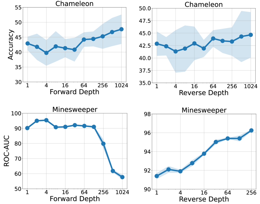
Figure 2: Prediction performance with varying numbers of forward and reverse layers. We vary the number of layers in one direction. Due to memory constraints, we restricted the reverse depth used in Minesweeper to 256 or less.

Over-Smoothing Analysis

We evaluate whether the proposed reverse diffusion mitigates the over-smoothing issue. To measure the degree of over-smoothing, we adopt Graph Smoothness Level (GSL) proposed by Zhang et al. (2022) defined as:

$$\operatorname{GSL}(\mathbf{X})=\frac{1}{N(N-1)}\sum_{i\in\mathcal{V}}\sum_{j\in\mathcal{V},j\neq i}\frac{\mathbf{x}_{i}\cdot\mathbf{x}_{j}}{\lVert{\mathbf{x}_{i}}\rVert_{F}\lVert{\mathbf{x}_{j}}\rVert_{F}},\;$$ (7)

where $\mathbf{x}_{i}$ is the representation of node $i$. The GSL represents the average cosine similarity across all pairs of nodes in the graph. A GSL value closer to one indicates more severe over-smoothing.

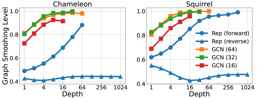
Figure 3: Over smoothing levels measured by GSL over the number of layers. Rep (forward) denotes the measured GSL in the forward process of GCN+ReP. We compare the results with GCN of three different numbers of layers: 16, 32, 64.

Figure 3 shows GSL of GCN+ReP and GCN with varying numbers of layers on Squirrel and Chameleon datasets. In both datasets, the GSL of GCN+ReP remains below 0.6 up to 1024 reverse layers, whereas the learned representations from GCN with 32 and 64 layers tend to become similar even after eight layers. GCN with 16 layers shows relatively low GSL values yet still exceeds 0.9 after eight layers. Compared with CGN, GCN+ReP shows relatively less GSL, showing that the reverse process can mitigate the over-smoothing in the forward processes as well.

Qualitative Analysis on Minesweeper Dataset

To validate that the reverse process produces a sharpened representation, we visualize label predictions on the Minesweeper dataset. The Minesweeper dataset is a binary classification task on a grid-structured graph, where the node with a positive label indicates the location of a mine. Each node, unless located on the boundaries, is connected to eight adjacent nodes, including the ones in the diagonal directions. The node feature is initialized with the number of mines in the adjacent nodes, and a one-hot representation of the feature is used as an initial representation of the node for learning.

Based on the representations obtained from the forward and reverse processes, we trained a GCN+ReP model with a single-layer MLP as a prediction head. In Figure 4, we visualize the prediction results of two randomly sampled $7\times 7$ sub-grids from $100\times 100$ grid structure. For each example, we visualize the prediction results with node representations from 1) forward process, 2) reverse process, 3) both directions and 4) true labels displayed from upper left to lower right. Since the prediction head needs concatenated representations for prediction, to visualize the prediction results focused on a forward or reverse representation, we set the other node representation to be zero, e.g., to predict the mine using node representation at layer $\ell>0$, $(\mathbf{X}^{(\ell)}\|\mathbf{0})$ is fed into the prediction head.

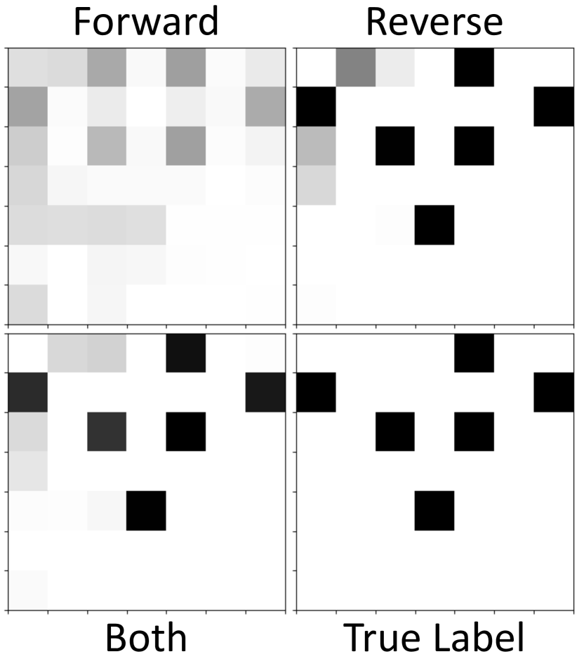
(a) Example 1

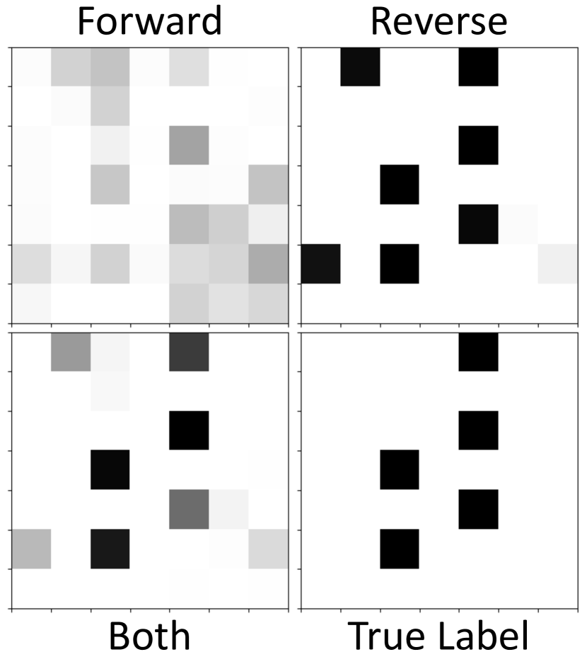
(b) Example 2

Figure 4: Visualization of node prediction on the minesweeper dataset. We visualize the prediction from 1) forward, 2) reverse, and 3) both representations, along with the ground truth labels.

In both examples, the prediction results from the reverse process appear sharper while those from the forward process tend to be smooth. Additionally, the sharp prediction created by the reverse process significantly contributes to label prediction. Although in some cases, the reverse process can perfectly classify the location of mines, e.g., example 1, the other cases require representations from both directions to classify the mines correctly, e.g., example 2.

Figure 1 shows the changes in predictions over the number of layers. The darker the cell, the higher the predicted probability of a mine being present. As expected, the predictions and representations therein tend to be sharp as the number of reverse layers increases.

4.2 Prediction with Low Label Rate

We compare node classification performance in citation graphs with low label rates, used to mimic the long-range dependencies between nodes. According to Zhao & Akoglu (2020), typical datasets are generally sufficient for shallow architectures, making it difficult to identify the advantages of deep GNNs. As explained by Sun et al. (2020), in scenarios with a low training label rate, more layers are necessary to access distant supervision.

We perform node label classification tasks on the Cora, Citeseer, and Pubmed datasets, with 20 labels per class in the training set. The validation and test sets were consistently set to 500 and 1,000, respectively. Each experiment was conducted across ten random splits of the dataset, with the mean and standard deviation of the results being reported.

We compare node classification accuracy on three citation datasets, Cora, CiteSeer, and PubMed, with baseline methods including GCN and GRAND++ (Thorpe et al., 2022) which is proposed especially for low-labeling rate problems.

Table 4 shows the average accuracy and standard deviation. We find that performance improves when ReP applied. The reverse process is even more effective than GRAND++, a model tailored for the low-rate label prediction task.

	Cora	CiteSeer	PubMed
GRAND++	72.18±3.10	64.31±1.91	75.94±2.50
GCN	76.50±1.77	61.67±3.30	76.25±2.36
GCN+ReP	79.06±1.54	66.46±1.82	76.92±1.34

Table 4: Prediction accuracy on the citation graphs with 20-label-per-class.

4.3 Run Time Analysis

We first measure how many iterations are required for the fixed point iterations to be converged. Figure 5 shows the difference between consecutive representations over the fixed point iterations with two datasets in terms of mean absolute difference. As shown in the figure, the fixed point method converges after seven iterations in general. In addition, we measure the training time for a single epoch and plot the results in Figure 6. The results show that the training time increases linearly as we increase the number of reverse layers coincided with the complexity analysis in Section 3.3.

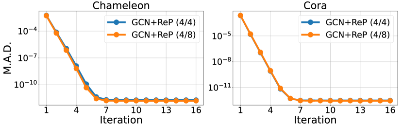
Figure 5: The mean absolute difference between two consecutive representations in the fixed-point method.

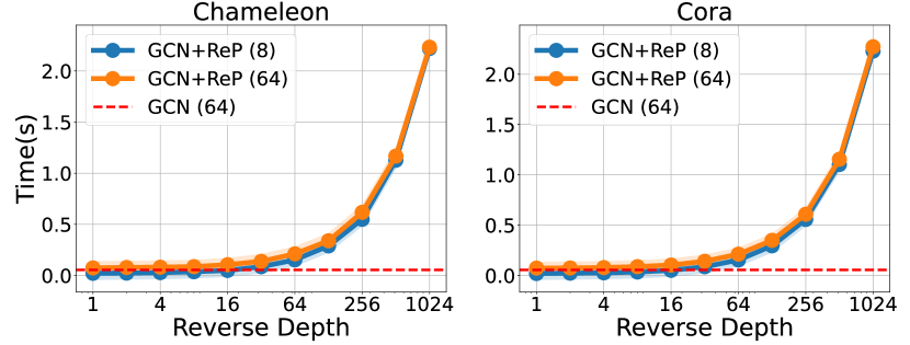
Figure 6: Average training time for the single epoch. The number of forward layers are shown next to the model.

5 Conclusion

In this work, we propose a reverse process for the message-passing-based graph neural networks. Through extensive empirical analysis, we have found that the reverse process can mitigate over-smoothing issues and allow long-distance nodes to interact with each other. Especially for the heterophilic datasets where the long-range interaction is necessary for a better prediction, the proposed method achieves outstanding results against many baseline models.

Future Work

To ensure invertibility, the Lipschitz constant of the forward process must be restricted to less than one, and the hidden dimension of weight parameters must remain constant. These restrictions limit the representation power and design choices within our framework. Investigating less restrictive invertible forms could lead to performance improvements.

Impact Statement

This paper presents work whose goal is to advance the field of Machine Learning. There are many potential societal consequences of our work, none of which we feel must be specifically highlighted here.

Appendix A Complexity Analysis

The method for calculating the forward process and the reverse process, when applied to a GCN with residual connections and weight sharing, is as follows:

$$\mathbf{X}^{(\ell+1)}=\mathbf{X}^{(\ell)}+\hat{\mathbf{A}}\mathbf{X}^{(\ell)}\mathbf{W},$$ (forward process) (8)

$$\mathbf{X}^{(\ell-1)}=\mathbf{X}^{(\ell)}+\sum_{k=1}^{K}(-1)^{k}\hat{\mathbf{A}}^{k}\mathbf{X}^{(\ell)}\mathbf{W}^{k},$$ (reverse process) (9)

For simplicity, we ignore an activation function.

A.1 Forward Pass of Forward Process

Equation 8 involves three key operations: matrix multiplication between $\mathbf{X}$ and $\mathbf{W}$ with complexity $O(|\mathcal{V}|d^{2})$, matrix multiplication between sparse matrix $\hat{\mathbf{A}}$ and $\mathbf{X}^{(\ell)}\mathbf{W}$ with complexity $O(|\mathcal{E}|d)$, and matrix addition with complexity $O(|\mathcal{V}|d)$. Overall, the time complexity for one-layer is $O(|\mathcal{V}|d^{2}+|\mathcal{E}|d)$. This results in a total time complexity of $O(L_{D}|\mathcal{V}|d^{2}+L_{D}|\mathcal{E}|d)$ over $L_{D}$ layers. Memory cost is calculated as $O(L_{D}|\mathcal{V}|d+|\mathcal{E}|+d^{2})$.

A.2 Backward Pass of Reverse Process

The time complexity of the backward pass primarily hinges on the computation of $\frac{\partial\mathcal{L}}{\partial\mathbf{W}}$. By applying the chain rule, this can be expressed as:

$$\frac{\partial\mathcal{L}}{\partial\mathbf{W}}=\frac{\partial\mathcal{L}}{\partial\mathbf{X}^{(L_{D})}}\frac{\partial\mathbf{X}^{(L_{D})}}{\partial\mathbf{X}^{(L_{D}-1)}}\cdots\frac{\partial\mathbf{X}^{(2)}}{\partial\mathbf{X}^{(1)}}\frac{\partial\mathbf{X}^{(1)}}{\partial\mathbf{W}}.$$ (10)

Given $\frac{\partial\mathcal{L}}{\partial\mathbf{X}^{(\ell)}}$, $\frac{\partial\mathcal{L}}{\partial\mathbf{X}^{(\ell-1)}}$ can be derived as follows:

$$\frac{\partial\mathcal{L}}{\partial\mathbf{X}^{(\ell-1)}}=\frac{\partial\mathcal{L}}{\partial\mathbf{X}^{(\ell)}}\frac{\partial\mathbf{X}^{(\ell)}}{\partial\mathbf{X}^{(\ell-1)}} =\frac{\partial\mathcal{L}}{\partial\mathbf{X}^{(\ell)}}\left(\frac{\partial}{\partial\mathbf{X}^{(\ell-1)}}\mathbf{I}\mathbf{X}^{(\ell-1)}+\frac{\partial}{\partial\mathbf{X}^{(\ell-1)}}\hat{\mathbf{A}}\mathbf{X}^{(\ell-1)}\mathbf{W}\right)$$

$$=\frac{\partial\mathcal{L}}{\partial\mathbf{X}^{(\ell)}}+\hat{\mathbf{A}}^{\top}\frac{\partial\mathcal{L}}{\partial\mathbf{X}^{(\ell)}}\mathbf{W}^{\top}.$$ (11)

And we can compute $\frac{\partial\mathcal{L}}{\partial\mathbf{X}^{(L_{D}-1)}}$ as follows:

$$\frac{\partial\mathcal{L}}{\partial\mathbf{X}^{(L_{D})}}\frac{\partial\mathbf{X}^{(L_{D})}}{\partial\mathbf{X}^{(L_{D}-1)}} =\frac{\partial\mathcal{L}}{\partial\mathbf{X}^{(L_{D})}}\left(\frac{\partial}{\partial\mathbf{X}^{(L_{D}-1)}}\mathbf{I}\mathbf{X}^{(L_{D}-1)}+\frac{\partial}{\partial\mathbf{X}^{(L_{D}-1)}}\hat{\mathbf{A}}\mathbf{X}^{(L_{D}-1)}\mathbf{W}\right)$$

$$=\frac{\partial\mathcal{L}}{\partial\mathbf{X}^{(L_{D})}}+\hat{\mathbf{A}}^{\top}\frac{\partial\mathcal{L}}{\partial\mathbf{X}^{(L_{D})}}\mathbf{W}^{\top}.$$ (12)

By recursively applying Equation 11 to Equation 12, we can obtain $\frac{\partial\mathcal{L}}{\partial\mathbf{X}^{(1)}}$ as follows:

$$\frac{\partial\mathcal{L}}{\partial\mathbf{X}^{(L_{D})}}\frac{\partial\mathbf{X}^{(L_{D})}}{\partial\mathbf{X}^{(L_{D}-1)}}\cdots\frac{\partial\mathbf{X}^{(2)}}{\partial\mathbf{X}^{(1)}}=\sum_{\ell=0}^{L_{D}-1}\binom{L_{D}-1}{\ell}({\hat{\mathbf{A}}^{\top}})^{\ell}\left(\frac{\partial\mathcal{L}}{\partial\mathbf{X}^{(L_{D})}}\right)({\mathbf{W}^{\top}})^{\ell}.$$ (13)

Finally, $\frac{\partial\mathcal{L}}{\partial\mathbf{W}}$ can be derived as the multiplication of $\frac{\partial\mathcal{L}}{\partial\mathbf{X}^{(1)}}$ and $\frac{\partial\mathbf{X}^{(1)}}{\partial\mathbf{W}}$:

$$\frac{\partial\mathcal{L}}{\partial\mathbf{W}} =\bigg{(}\sum_{\ell=0}^{L_{D}-1}\binom{L_{D}-1}{\ell}({\hat{\mathbf{A}}^{\top}})^{\ell}\left(\frac{\partial\mathcal{L}}{\partial\mathbf{X}^{(L_{D})}}\right)({\mathbf{W}^{\top}})^{\ell}\bigg{)}\left(\frac{\partial}{\partial\mathbf{W}}\hat{\mathbf{A}}\mathbf{X}^{(0)}\mathbf{W}\right)$$

$$=\left(\hat{\mathbf{A}}\mathbf{X}^{(0)}\right)^{\top}\bigg{(}\sum_{\ell=0}^{L_{D}-1}\binom{L_{D}-1}{\ell}({\hat{\mathbf{A}}^{\top}})^{\ell}\left(\frac{\partial\mathcal{L}}{\partial\mathbf{X}^{(L_{D})}}\right)({\mathbf{W}^{\top}})^{\ell}\bigg{)}.$$ (14)

Note that $\hat{\mathbf{A}}$ is the sparse matrix, so matrix multiplication can be performed in $O(|\mathcal{E}|d)$. So, the time complexity of the term in the summation is $O(|\mathcal{V}|d^{2}+\ell d^{3}+\ell|\mathcal{E}|d)$. Thus, the time complexity for computing $\frac{\partial\mathcal{L}}{\partial\mathbf{W}}$ is $O(L_{D}|\mathcal{V}|d^{2}+L_{D}^{2}d^{3}+L_{D}^{2}|\mathcal{E}|d)$, with a memory cost of $O(|\mathcal{V}|d+|\mathcal{E}|+d^{2})$.

A.3 Forward Pass of Reverse Process

To calculate Equation 9, the initial step involves computing $(-1)^{k}\hat{\mathbf{A}}^{k}\mathbf{X}^{(\ell)}\mathbf{W}^{k}$. The time complexity for this part is $O(k|\mathcal{E}|d+|\mathcal{V}|d^{2}+kd^{3})$. Summing over $k$ from 0 to $K$, the overall complexity becomes $O(K^{2}|\mathcal{E}|d+K|\mathcal{V}|d^{2}+K^{2}d^{3})$. With $L_{R}$ representing the number of reverse process layers, the total time complexity is calculated as $O(K^{2}L_{R}|\mathcal{E}|d+KL_{R}|\mathcal{V}|d^{2}+K^{2}L_{R}d^{3})$.

A.4 Backward Pass of Reverse Process

The time complexity of the backward pass primarily hinges on the computation of $\frac{\partial\mathcal{L}}{\partial\mathbf{W}}$. By applying the chain rule, this can be expressed as:

$$\frac{\partial\mathcal{L}}{\partial\mathbf{W}}=\frac{\partial\mathcal{L}}{\partial\mathbf{X}^{(-L_{R})}}\frac{\partial\mathbf{X}^{(-L_{R})}}{\partial\mathbf{X}^{(-L_{R}+1)}}\cdots\frac{\partial\mathbf{X}^{(-2)}}{\partial\mathbf{X}^{(-1)}}\frac{\partial\mathbf{X}^{(-1)}}{\partial\mathbf{W}}.$$ (15)

Given $\frac{\partial\mathcal{L}}{\partial\mathbf{X}^{(\ell)}}$, $\frac{\partial\mathcal{L}}{\partial\mathbf{X}^{(\ell+1)}}$ can be derived as follows:

$$\frac{\partial\mathcal{L}}{\partial\mathbf{X}^{(\ell+1)}}=\frac{\partial\mathcal{L}}{\partial\mathbf{X}^{(\ell)}}\frac{\partial\mathbf{X}^{(\ell)}}{\partial\mathbf{X}^{(\ell+1)}} =\frac{\partial\mathcal{L}}{\partial\mathbf{X}^{(\ell)}}\frac{\partial}{\partial\mathbf{X}^{(\ell+1)}}\left(\mathbf{X}^{(\ell+1)}+\sum_{k=1}^{K}(-1)^{k}\hat{\mathbf{A}}^{k}\mathbf{X}^{(\ell+1)}\mathbf{W}^{k}\right)$$

$$=\frac{\partial\mathcal{L}}{\partial\mathbf{X}^{(\ell)}}+\sum_{k=1}^{K}(-1)^{k}\left(\hat{\mathbf{A}}^{k}\right)^{\top}\frac{\partial\mathcal{L}}{\partial\mathbf{X}^{(\ell)}}\left(\mathbf{W}^{k}\right)^{\top}.$$ (16)

And we can compute $\frac{\partial\mathcal{L}}{\partial\mathbf{X}^{(-L_{R}+1)}}$ as follows:

$$\frac{\partial\mathcal{L}}{\partial\mathbf{X}^{(-L_{R}+1)}}=\frac{\partial\mathcal{L}}{\partial\mathbf{X}^{(-L_{R})}}\frac{\partial\mathbf{X}^{(-L_{R})}}{\partial\mathbf{X}^{(-L_{R}+1)}} =\frac{\partial\mathcal{L}}{\partial\mathbf{X}^{(-L_{R})}}\frac{\partial}{\partial\mathbf{X}^{(-L_{R}+1)}}\left(\mathbf{X}^{(-L_{R}+1)}+\sum_{k=1}^{K}(-1)^{k}\hat{\mathbf{A}}^{k}\mathbf{X}^{(-L_{R}+1)}\mathbf{W}^{k}\right)$$

$$=\frac{\partial\mathcal{L}}{\partial\mathbf{X}^{(-L_{R})}}+\sum_{k=1}^{K}(-1)^{k}\left(\hat{\mathbf{A}}^{k}\right)^{\top}\frac{\partial\mathcal{L}}{\partial\mathbf{X}^{(-L_{R})}}\left(\mathbf{W}^{k}\right)^{\top}.$$ (17)

By recursively applying Equation 16 to Equation 17, we can obtain $\frac{\partial\mathcal{L}}{\partial\mathbf{X}^{(-1)}}$ as follows:

$$\frac{\partial\mathcal{L}}{\partial\mathbf{X}^{(-L_{R})}}\frac{\partial\mathbf{X}^{(-L_{R})}}{\partial\mathbf{X}^{(-L_{R}+1)}}\cdots\frac{\partial\mathbf{X}^{(-2)}}{\partial\mathbf{X}^{(-1)}}$$

$$= \frac{\partial\mathcal{L}}{\partial\mathbf{X}^{(-L_{R})}}+\sum_{\ell=2}^{L_{R}-1}\binom{L_{R}-1}{\ell}\sum_{(k_{1},k_{2},\cdots,k_{\ell-1})}(-1)^{\sum_{i=1}^{\ell-1}k_{i}}({\hat{\mathbf{A}}^{\top}})^{\sum_{i=1}^{\ell-1}k_{i}}\left(\frac{\partial\mathcal{L}}{\partial\mathbf{X}^{(-L_{R})}}\right)({\mathbf{W}^{\top}})^{\sum_{i=1}^{\ell-1}k_{i}}.$$ (18)

In addition, $\frac{\partial\mathbf{X}^{(-1)}}{\partial\mathbf{W}}$ can be obtained as follows:

$$\frac{\partial\mathbf{X}^{(-1)}}{\partial\mathbf{W}} =\frac{\partial}{\partial\mathbf{W}}\left(\mathbf{X}^{(0)}+\sum_{k_{0}=1}^{K}(-1)^{k_{0}}\hat{\mathbf{A}}^{k_{0}}\mathbf{X}^{(0)}\mathbf{W}^{k_{0}}\right)$$

$$=\sum_{k_{0}=1}^{K}(-1)^{k_{0}}k_{0}\frac{\partial}{\partial\mathbf{W}^{k_{0}}}(\hat{\mathbf{A}}^{k_{0}}\mathbf{X}^{(0)}\mathbf{W}^{k_{0}})\mathbf{W}^{k_{0}-1}\frac{\partial\mathbf{W}}{\partial\mathbf{W}}.$$ (19)

Finally, $\frac{\partial\mathcal{L}}{\partial\mathbf{W}}$ can be derived as the multiplication of $\frac{\partial\mathcal{L}}{\partial\mathbf{X}^{(-1)}}$ and $\frac{\partial\mathbf{X}^{(-1)}}{\partial\mathbf{W}}$:

$$\frac{\partial\mathcal{L}}{\partial\mathbf{W}} =\sum_{k_{0}=1}^{K}\Bigg{[}(-1)^{k_{0}}k_{0}(\hat{\mathbf{A}}^{k_{0}}\mathbf{X}^{(0)})^{\top}\left(\frac{\partial\mathcal{L}}{\partial\mathbf{X}^{(-L_{R})}}\right)\mathbf{W}^{k_{0}-1}$$

$$+\sum_{\ell=2}^{L_{R}-1}\binom{L_{R}-1}{\ell}\sum_{(k_{1},k_{2},\cdots,k_{\ell-1})}(-1)^{\sum_{i=1}^{\ell-1}k_{i}}k_{0}(\hat{\mathbf{A}}^{k_{0}}\mathbf{X}^{(0)})^{\top}({\hat{\mathbf{A}}^{\top}})^{\sum_{i=1}^{\ell-1}k_{i}}\left(\frac{\partial\mathcal{L}}{\partial\mathbf{X}^{(-L_{R})}}\right)({\mathbf{W}^{\top}})^{\sum_{i=1}^{\ell-1}k_{i}}\mathbf{W}^{k_{0}-1}\Bigg{]}.$$ (20)

By the same procedure in the forward process, the time complexity of the first term in brackets is $O(k_{0}(|\mathcal{E}|d+d^{3})+|\mathcal{V}|d^{2})$. In the case of the second term, there are up to $2\ell K$ possible outcomes for $\sum_{i=1}^{\ell}k_{i}$. So the time complexity is $O(L_{R}+K\ell|\mathcal{V}|d^{2}+\ell^{2}K^{2}(d^{3}+|\mathcal{E}|d))$. So the overall time complexity of reverse process is $O((L_{D}^{2}+M^{2}L_{R}^{3})|\mathcal{E}|d+(L_{D}^{2}+ML_{R}^{2})|\mathcal{V}|d^{2}+M^{2}L_{R}^{3}d^{3})$. The memory complexity is $O(|\mathcal{V}|d+|\mathcal{E}|+d^{2})$.

Appendix B Dataset Statistics

Table 5 presents the dataset statistics utilized in experiments. There are two forms of homophily: edge homophily (Abu-El-Haija et al., 2019; Zhu et al., 2020) and adjusted homophily (Platonov et al., 2023a). Edge homophily denotes the proportion of edges connecting nodes with the same label, formally expressed as:

$$h_{\text{edge }}=\frac{\left.\mid(u,v)\in E:y_{u}=y_{v}\right\}\mid}{|E|},$$

where $E$ is the set of edges, and $y_{n}$ is the label of node $n$. However, edge homophily is acknowledged to be meaningless in graphs with imbalanced labels. To address this issue, adjusted homophily is introduced. Formally, adjusted homophily is defined as:

$$h_{adj}=\frac{h_{\text{edge }}-\sum_{k=1}^{C}D_{k}^{2}/(2|E|)^{2}}{1-\sum_{k=1}^{C}D_{k}^{2}/(2|E|)^{2}},$$

where $D_{k}$ is the total degree of nodes of class $k$, and $C$ is the number of classes. We employed seven heterophilic datasets characterized by low adjusted homophily and five commonly used homophilic datasets exhibiting high edge homophily and adjusted homophily.

Dataset	# nodes	# edges	# classes	avg degree	edge homophily	adjusted homophily
Squirrel-filtered	2,223	46,998	5	42.28	0.21	0.01
Chameleon-filtered	890	8,854	5	19.90	0.24	0.03
roman-empire	22,662	32,927	18	2.91	0.05	-0.05
amazon-ratings	24,492	93,050	5	7.60	0.38	0.14
minesweeper	10,000	39,402	2	7.88	0.68	0.01
tolokers	11,758	519,000	2	88.28	0.59	0.09
questions	48,921	153,540	2	6.28	0.84	0.02
Cora	2,708	5,278	7	3.90	0.81	0.77
CiteSeer	3,327	4,552	6	2.74	0.74	0.67
PubMed	19,717	44,324	3	4.50	0.80	0.69
Computers	13,752	245,861	10	35.76	0.78	0.68
Photo	7,650	119,081	8	31.13	0.83	0.79

Table 5: Statistics of the dataset utilized in the experiments.

Appendix C Multi-head Attention for GAT

GAT calculates an attention matrix as follows:

$$\hat{A}_{ij}=\frac{\exp\left(\operatorname{LeakyReLU}\left(\mathbf{a}^{\top}\left[\mathbf{W}^{\top}\mathbf{X}_{i}\|\mathbf{W}^{\top}\mathbf{X}_{j}\right]\right)\right)}{\sum_{k\in\mathcal{N}_{i}}\exp\left(\operatorname{LeakyReLU}\left(\mathbf{a}^{\top}\left[\mathbf{W}^{\top}\mathbf{X}_{i}\|\mathbf{W}^{\top}\mathbf{X}_{j}\right]\right)\right)},\;$$ (21)

where $\mathbf{a}\in\mathbb{R}^{2d}$ is a learnable parameter. Our framework also adopts averaging when using multi-head attention and remains hidden dimension constant to ensure invertibility, resulting in:

$$h(\mathbf{X}^{(\ell)})=\sigma(\frac{1}{K}\sum_{k=1}^{K}\hat{\mathbf{A}}^{(k)}\mathbf{X}^{(\ell)}\mathbf{W}^{(k)}).\;$$ (22)

In this case, the upper bound of the Lipschitz constant of $h$ is calculated as follows:

$$\text{Lip}(h) =\sup_{\mathbf{X}\neq\mathbf{0}}\frac{\lVert{\frac{1}{K}\sum_{k=1}^{K}\hat{\mathbf{A}}^{(k)}\mathbf{X}^{(\ell)}\mathbf{W}^{(k)}}\rVert_{F}}{\lVert{\mathbf{X}}\rVert_{F}}$$ (23)

$$\leq\frac{1}{K}\sum_{k=1}^{K}\sup_{\mathbf{X}\neq\mathbf{0}}\frac{\lVert{\hat{\mathbf{A}}^{(k)}\mathbf{X}^{(\ell)}}\rVert_{F}}{\lVert{\mathbf{X}}\rVert_{F}}\lVert{\mathbf{W}^{(k)}}\rVert_{F}$$ (24)

$$\leq\frac{1}{K}\sum_{k=1}^{K}\lVert{\mathbf{W}^{(k)}}\rVert_{F},\;$$ (25)

since $\lVert{\sum\mathbf{X}}\rVert_{F}\leq\sum\lVert{\mathbf{X}}\rVert_{F}$.

Appendix D Full Results of Homophily Datasets

We provide the experimental results of all homophilic datasets in Table 6.

	Cora	CiteSeer	PubMed	Computers	Photo
MLP*	76.96±0.95	76.58±0.88	85.94±0.22	82.85±0.38	84.72±0.34
vanilla-GCN*	87.14±1.01	79.86±0.67	86.74±0.27	83.32±0.33	88.26±0.73
vanilla-GAT*	88.03±0.79	80.52±0.71	87.04±0.24	83.32±0.39	90.94±0.68
APPNP*	88.14±0.73	80.47±0.74	88.12±0.31	85.32±0.37	88.51±0.31
ChevNet*	86.67±0.82	79.11±0.75	87.95±0.28	87.54±0.43	93.77±0.32
GPR-GNN*	88.57±0.69	80.12±0.83	88.46±0.33	86.85±0.25	93.85±0.28
BernNet*	88.52±0.95	80.09±0.79	88.48±0.41	87.64±0.44	93.63±0.35
GRAND	85.53±0.64	74.95±1.37	88.81±0.69	90.28±0.47	94.01±0.73
GRAND+ReP	85.73±1.39	75.78±1.48	89.03±0.61	89.51±0.78	94.48±0.61
$\Delta$	$+0.20\;(\uparrow)$	$+0.83\;(\uparrow)$	$+0.22\;(\uparrow)$	$-0.77\;(\downarrow)$	$+0.47\;(\uparrow)$
GAT	87.67±0.84	77.36±1.59	89.66±0.60	92.15±0.30	95.86±0.58
GAT+ReP	87.93±1.60	77.06±1.60	89.94±0.61	91.03±0.62	95.44±0.71
	$(64/32)$	$(32/128)$	$(8/8)$	$(16/8)$	$(32/8)$
$\Delta$	$+0.26(\uparrow)$	$-0.30(\downarrow)$	$+0.28(\uparrow)$	$-1.12(\downarrow)$	$-0.42(\downarrow)$
GCN	88.00±1.42	77.15±1.44	89.37±0.52	91.87±0.57	95.35±0.47
GCN+ReP	87.63±1.40	77.33±1.65	89.96±0.55	90.92±0.52	95.50±0.63
	$(32/512)$	$(8/32)$	$(32/32)$	$(32/64)$	$(32/128)$
$\Delta$	$-0.37(\downarrow)$	$+0.18(\uparrow)$	$+0.59(\uparrow)$	$-0.95(\downarrow)$	$+0.15(\uparrow)$

Table 6: Test accuracy and standard deviation on homophilic datasets. $\Delta$ indicates the difference with and without ReP. We also report the number of forward and reverse layers below the performance of GCN$+$ReP and GAT$+$ReP. The best and the second-best are bolded and underlined, respectively.

References

- Abu-El-Haija et al. (2019) Abu-El-Haija, S., Perozzi, B., Kapoor, A., Alipourfard, N., Lerman, K., Harutyunyan, H., Ver Steeg, G., and Galstyan, A. Mixhop: Higher-order graph convolutional architectures via sparsified neighborhood mixing. In international conference on machine learning, pp. 21–29. PMLR, 2019.
- Azabou et al. (2023) Azabou, M., Ganesh, V., Thakoor, S., Lin, C.-H., Sathidevi, L., Liu, R., Valko, M., Veličković, P., and Dyer, E. L. Half-hop: a graph upsampling approach for slowing down message passing. In Proceedings of the 40th International Conference on Machine Learning, ICML’23. JMLR.org, 2023.
- Behrmann et al. (2019) Behrmann, J., Grathwohl, W., Chen, R. T. Q., Duvenaud, D., and Jacobsen, J.-H. Invertible residual networks. In Chaudhuri, K. and Salakhutdinov, R. (eds.), Proceedings of the 36th International Conference on Machine Learning, volume 97 of Proceedings of Machine Learning Research, pp. 573–582. PMLR, 09–15 Jun 2019.
- Bo et al. (2021) Bo, D., Wang, X., Shi, C., and Shen, H. Beyond low-frequency information in graph convolutional networks. In Proceedings of the AAAI Conference on Artificial Intelligence, volume 35, pp. 3950–3957, 2021.
- Chamberlain et al. (2021) Chamberlain, B., Rowbottom, J., Gorinova, M. I., Bronstein, M., Webb, S., and Rossi, E. Grand: Graph neural diffusion. In Meila, M. and Zhang, T. (eds.), Proceedings of the 38th International Conference on Machine Learning, volume 139 of Proceedings of Machine Learning Research, pp. 1407–1418. PMLR, 18–24 Jul 2021.
- Chen et al. (2018) Chen, R. T. Q., Rubanova, Y., Bettencourt, J., and Duvenaud, D. K. Neural ordinary differential equations. In Bengio, S., Wallach, H., Larochelle, H., Grauman, K., Cesa-Bianchi, N., and Garnett, R. (eds.), Advances in Neural Information Processing Systems, volume 31. Curran Associates, Inc., 2018. URL https://proceedings.neurips.cc/paper_files/paper/2018/file/69386f6bb1dfed68692a24c8686939b9-Paper.pdf.
- Chien et al. (2020) Chien, E., Peng, J., Li, P., and Milenkovic, O. Adaptive universal generalized pagerank graph neural network. arXiv preprint arXiv:2006.07988, 2020.
- Defferrard et al. (2016) Defferrard, M., Bresson, X., and Vandergheynst, P. Convolutional neural networks on graphs with fast localized spectral filtering. Advances in neural information processing systems, 29, 2016.
- Du et al. (2022) Du, L., Shi, X., Fu, Q., Ma, X., Liu, H., Han, S., and Zhang, D. Gbk-gnn: Gated bi-kernel graph neural networks for modeling both homophily and heterophily. In Proceedings of the ACM Web Conference 2022, pp. 1550–1558, 2022.
- Gasteiger et al. (2018) Gasteiger, J., Bojchevski, A., and Günnemann, S. Predict then propagate: Graph neural networks meet personalized pagerank. arXiv preprint arXiv:1810.05997, 2018.
- Hamilton et al. (2017) Hamilton, W., Ying, Z., and Leskovec, J. Inductive representation learning on large graphs. Advances in neural information processing systems, 30, 2017.
- He et al. (2016) He, K., Zhang, X., Ren, S., and Sun, J. Deep residual learning for image recognition. In 2016 IEEE Conference on Computer Vision and Pattern Recognition (CVPR), pp. 770–778, Los Alamitos, CA, USA, jun 2016. IEEE Computer Society. URL https://doi.ieeecomputersociety.org/10.1109/CVPR.2016.90.
- He et al. (2021) He, M., Wei, Z., Huang, Z., and Xu, H. Bernnet: Learning arbitrary graph spectral filters via bernstein approximation. In Beygelzimer, A., Dauphin, Y., Liang, P., and Vaughan, J. W. (eds.), Advances in Neural Information Processing Systems, 2021. URL https://openreview.net/forum?id=WigDnV-_Gq.
- Kipf & Welling (2017) Kipf, T. N. and Welling, M. Semi-supervised classification with graph convolutional networks. In International Conference on Learning Representations, 2017. URL https://openreview.net/forum?id=SJU4ayYgl.
- Li et al. (2022) Li, X., Zhu, R., Cheng, Y., Shan, C., Luo, S., Li, D., and Qian, W. Finding global homophily in graph neural networks when meeting heterophily. In International Conference on Machine Learning, pp. 13242–13256. PMLR, 2022.
- Liang et al. (2023) Liang, L., Hu, X., Xu, Z., Song, Z., and King, I. Predicting global label relationship matrix for graph neural networks under heterophily. In Thirty-seventh Conference on Neural Information Processing Systems, 2023.
- Maurya et al. (2022) Maurya, S. K., Liu, X., and Murata, T. Simplifying approach to node classification in graph neural networks. Journal of Computational Science, 62:101695, 2022.
- Platonov et al. (2023a) Platonov, O., Kuznedelev, D., Babenko, A., and Prokhorenkova, L. Characterizing graph datasets for node classification: Homophily-heterophily dichotomy and beyond. In The Second Learning on Graphs Conference, 2023a.
- Platonov et al. (2023b) Platonov, O., Kuznedelev, D., Diskin, M., Babenko, A., and Prokhorenkova, L. A critical look at evaluation of gnns under heterophily: Are we really making progress? In The Eleventh International Conference on Learning Representations, 2023b.
- Rong et al. (2020) Rong, Y., Huang, W., Xu, T., and Huang, J. Dropedge: Towards deep graph convolutional networks on node classification. In International Conference on Learning Representations, 2020. URL https://openreview.net/forum?id=Hkx1qkrKPr.
- Shi et al. (2020) Shi, Y., Huang, Z., Feng, S., Zhong, H., Wang, W., and Sun, Y. Masked label prediction: Unified message passing model for semi-supervised classification. arXiv preprint arXiv:2009.03509, 2020.
- Song et al. (2023) Song, Y., Zhou, C., Wang, X., and Lin, Z. Ordered gnn: Ordering message passing to deal with heterophily and over-smoothing. arXiv preprint arXiv:2302.01524, 2023.
- Sun et al. (2020) Sun, K., Lin, Z., and Zhu, Z. Multi-stage self-supervised learning for graph convolutional networks on graphs with few labeled nodes. In The Thirty-Fourth AAAI Conference on Artificial Intelligence, AAAI 2020, The Thirty-Second Innovative Applications of Artificial Intelligence Conference, IAAI 2020, The Tenth AAAI Symposium on Educational Advances in Artificial Intelligence, EAAI 2020, New York, NY, USA, February 7-12, 2020, 2020. URL https://doi.org/10.1609/aaai.v34i04.6048.
- Thorpe et al. (2022) Thorpe, M., Nguyen, T. M., Xia, H., Strohmer, T., Bertozzi, A., Osher, S., and Wang, B. Grand++: Graph neural diffusion with a source term. In International Conference on Learning Representation (ICLR), 2022.
- Veličković et al. (2018) Veličković, P., Cucurull, G., Casanova, A., Romero, A., Liò, P., and Bengio, Y. Graph attention networks. In International Conference on Learning Representations, 2018. URL https://openreview.net/forum?id=rJXMpikCZ.
- Wang & Zhang (2022) Wang, X. and Zhang, M. How powerful are spectral graph neural networks. In International Conference on Machine Learning, pp. 23341–23362. PMLR, 2022.
- Zhang et al. (2022) Zhang, W., Sheng, Z., Yin, Z., Jiang, Y., Xia, Y., Gao, J., Yang, Z., and Cui, B. Model degradation hinders deep graph neural networks. In Proceedings of the 28th ACM SIGKDD Conference on Knowledge Discovery and Data Mining, 2022. URL https://doi.org/10.1145/3534678.3539374.
- Zhao & Akoglu (2020) Zhao, L. and Akoglu, L. Pairnorm: Tackling oversmoothing in gnns. In International Conference on Learning Representations, 2020. URL https://openreview.net/forum?id=rkecl1rtwB.
- Zhu et al. (2020) Zhu, J., Yan, Y., Zhao, L., Heimann, M., Akoglu, L., and Koutra, D. Beyond homophily in graph neural networks: Current limitations and effective designs. Advances in neural information processing systems, 33:7793–7804, 2020.
- Zhu et al. (2021) Zhu, J., Rossi, R. A., Rao, A., Mai, T., Lipka, N., Ahmed, N. K., and Koutra, D. Graph neural networks with heterophily. In Proceedings of the AAAI conference on artificial intelligence, volume 35, pp. 11168–11176, 2021.