The Graph Fractional Fourier Transform
in Hilbert Space

Abstract

Graph signal processing (GSP) leverages the inherent signal structure within graphs to extract high-dimensional data without relying on translation invariance. It has emerged as a crucial tool across multiple fields, including learning and processing of various networks, data analysis, and image processing. In this paper, we introduce the graph fractional Fourier transform in Hilbert space (HGFRFT), which provides additional fractional analysis tools for generalized GSP by extending Hilbert space and vertex domain Fourier analysis to fractional order. First, we establish that the proposed HGFRFT extends traditional GSP, accommodates graphs on continuous domains, and facilitates joint time-vertex domain transform while adhering to critical properties such as additivity, commutativity, and invertibility. Second, to process generalized graph signals in the fractional domain, we explore the theory behind filtering and sampling of signals in the fractional domain. Finally, our simulations and numerical experiments substantiate the advantages and enhancements yielded by the HGFRFT.

I Introduction

With the increasing amount of complex data on non-Euclidean spaces and irregular domains, the theories and applications of graph signal processing (GSP) have developed rapidly in recent years [1, 2, 3, 4, 5, 6, 7, 8, 9, 10, 11, 12, 13, 14, 15]. Under the GSP framework, two standard signal processing approaches [1, 2] have been adopted. The first approach is based on the concept of the Laplacian matrix [1], while the second, derived from algebraic signal processing, is based on the graph adjacency matrix, also known as the graph shift operator [2, 3].

In recent years, traditional time-frequency domain signal processing methods have been extended to the GSP field. These include sampling and interpolation [6, 7, 8], filtering [9], frequency analysis [10], signal reconstruction [11], uncertainty principle [12, 13], Fourier transform (FT) [1, 2, 14], and windowed Fourier transform [15] methods. The graph Fourier transform (GFT) is a generalization of the discrete Fourier transform (DFT) on graphs. As the application of DFT in the traditional time-frequency domain, the GFT has also found many applications in GSP, including denoising [16, 17], classification [6], clustering [16, 17, 18], spectral estimation [19], semisupervised learning [20], machine learning and deep learning [21, 22].

The traditional GSP theory [1, 2, 3, 4, 5] is based on the variation of the orthonormal basis in the finite-dimensional vector space. The graph signal $f$ assigns a real number to each vertex; thus, $f$ can be regarded as an element of $\mathbb{R}^{N}$, where $\mathbb{R}$ is the set of real numbers. However, whether the matrix is a Laplacian matrix or an adjacency matrix of the graph signals, all the eigenvalues are real numbers that form an orthonormal basis [23]. Most of the current research on graph signals is based on this, and more complex graph structures are rarely studied.

Nonetheless, irregular graph data in the GSP are primarily modeled using vertices and edges; instead of a real number being assigned at each vertex, a mathematical object with a richer structure can be assigned to each vertex of the graph. Ji and Tay [24, 25] proposed the creatively developed generalized GSP method in Hilbert space. In the framework of their method, the information in the Hilbert space can be processed jointly with the vertex domain. As the main joint Fourier analysis tool for obtaining the joint Hilbert space-vertex signal spectrum extension under this framework, the graph Fourier transform in Hilbert space (HGFT) is defined using the compact operator on the Hilbert space and the adjacency matrix on graphs. The HGFT combines the FT in Hilbert space and the GFT in the vertex domain, aiming to reduce signals in infinite continuous domains to form more manageable finite domains. Methods such as filtering [24, 25, 26, 27, 28], sampling [29, 30, 31] and estimation [32] can be included in this framework, which can be categorized based on three scenarios:

• When the vertices are assigned real numbers, it is the traditional GSP [1, 2, 3, 4, 5, 6, 7, 8, 9, 10, 11, 12, 13, 14, 15];

• When the vertices are assigned to a specified finite closed interval $[a,b]$ that satisfies the Lebesgue measure, it is a joint time-vertex GSP [16, 17];

• When the vertices are assigned a new graph structure that is in a Hilbert space and has a discrete metric in $L^{2}$ or $\ell^{2}$ space [24, 25, 26].

Although the HGFT can effectively perform basic graph frequency analysis under this framework, it requires the information of the entire graph signal in Hilbert space, which cannot be obtained using the conversion process from the Hilbert space-vertex domain to the graph frequency domain. Due to space constraints, the HGFT only uses surfaces in different applications [24] and is not able to process chirp signals on graphs, such as graph signals of complex numbers. Therefore, new generalized GSP methods must be found.

To address the above problems, we apply the fractional Fourier transform (FRFT) to the generalized GSP. The FRFT was proposed in 1980 [33] and introduced into the signal processing field in 1994 [34]. It is a generalization of the FT that rotates a signal into an intermediate domain between time and frequency. The FRFT can also be seen as extending a signal over a set of chirps. The FRFT provides an additional degree of freedom when a signal is transformed into the intermediate time-frequency domain while leaving ordinary FT as a special case. This property of the FRFT provides flexibility in data processing and improves performance, typically at no additional computational cost. Thus, similar to the extension of the FT to graph signals, the extension of the FRFT to graph signals enables further developments, application areas, and performance improvements.

The resulting graph fractional Fourier transform (GFRFT) [35] transforms the graph signal into the intermediate vertex frequency or vertex spectral domain. Furthermore, the windowed fractional Fourier transform and the linear canonical transform have been generalized to GSP [36, 37], and sampling [38], filtering [39], denoising [40] and classification [38] in the fractional domain have been studied.

Since the GFRFT [35] can observe the spectrum of the graph signal at different angles, it does not require information about the entire graph signal, and because of the existence of order $\alpha$, it has more flexibility than the GFT, making it more efficient for processing “graph chirp signals”. Therefore, introducing the GFRFT into the generalized GSP framework [24, 25] can enable the characteristics of the HGFT to be further studied and leveraged, which is interesting research. Applying fractional order to the joint Hilbert space-vertex signal spectrum analysis can enable signals with richer structures to be processed in the fractional domain, which is a current research direction. Similar to the FRFT, which generalizes the FT, we propose the graph fractional Fourier transform in Hilbert space (HGFRFT), which can analyze signals in both the graph fractional domain and the Hilbert space fractional domain. We also apply the framework to real datasets and develop adaptations for different scenarios of interest.

Contributions:

• The HGFRFT, which can analyze vertex signals under Hilbert space in a wider range of transformation categories, is proposed as a new approach for graph chirp signals;

• Some filters based on the HGFRFT for graph signals in Hilbert space are proposed, providing tools for GSP with richer structures in the fractional domain;

• A novel sampling operator based on the HGFRFT for graph signals in Hilbert space is proposed; this operator can solve complex Hilbert space-vertex domain sampling problems.

The remainder of this paper is organized as follows. In Section II, we provide preliminary information on the generalized GSP, GFRFT and HGFT. In Section III, we define the proposed HGFRFT and provide its properties and examples. In Sections IV and V, we introduce the HGFRFT-based filters and sampling theorem, respectively. In Section VI, we demonstrate the superiority of the HGFRFT in fractional sampling, frequency analysis and classification through simulation experiments and three applied numerical experiments. In Section VII, we conclude the paper.

Notations: We use $\mathbb{R}$, $\mathbb{C}$ and $\mathbb{Z}$ to denote the field of real numbers, field of complex numbers and set of integers, respectively. The symbols $\otimes$ and $\circ$ denote tensor product and function composition, respectively, while $\cong$ denotes isomorphism. $\mathbf{I}_{N}$ is an identity operator of size $N$, if there is no special size requirement, it can be simplified to $\mathbf{I}$. If $\mathbf{A}\in\mathbb{C}^{N\times N}$ and $\mathbf{B}\in\mathbb{C}^{M\times M}$ are square matrices, then $\mathbf{A}\otimes_{K}\mathbf{B}$ denotes their Kronecker product, where $\otimes_{K}$ acts on the matrix (so it can be regarded as a second-order tensor) and is a special form of tensor product. The space $L^{2}(\Omega)$ takes $(\Omega,\mathcal{F},\mu)$ as the measure space, and $\mathbb{C}^{N}$ is equipped with the inner product $\left<\cdot,\cdot\right>_{\mathbb{C}^{N}}$ and the corresponding norm $||\cdot||_{\mathbb{C}^{N}}$. This space is the set of functions $f:\Omega\mapsto\mathbb{C}$ such that $\int_{\Omega}\left|f\right|^{2}\mathrm{d}\mu<\infty$.

II Preliminaries

In traditional GSP, the signals on the vertices of $\mathcal{G}=(\mathcal{V},\mathcal{E})$ are assumed to be real or complex, where $\mathcal{V}$ is a vertex and $\mathcal{E}$ is an edge. Before extending the GFRFT to Hilbert space, we review the basic concepts and definitions of graph signals in Hilbert space, the GFRFT and the HGFT.

II-A Graph Signals in Hilbert Space

Let $\mathcal{G}$ be a simple finite undirected weighted graph and $\mathcal{H}$ be a Hilbert space (a complete inner product space). Given a function $f:\mathcal{V}\rightarrow\mathcal{H}$ denoted as a graph signal in $\mathcal{H}$, let $S(\mathcal{G},\mathcal{H})$ denote the graph signal space in $\mathcal{H}$ [24].

Hilbert spaces contain both finite-dimensional and infinite-dimensional cases, where more realistic signals can be represented in practice [41]. In most physical signals, $\mathcal{H}$ is separable if the signal has a countable orthonormal basis, and it can be assumed that for some measurable space $\Omega$, there is the measure $\mu$, and $\mathcal{H}=L^{2}\left(\Omega\right)$. For each $f\in S\left(\mathcal{G},\mathcal{H}\right)$ and $u\in\mathcal{V},f\left(u\right)\in L^{2}\left(\Omega\right)$ and $f$ can be regarded as a function of two variables, $f(u,x)=f(u)(x)\in\mathbb{C}$, for each $x\in\Omega$.

For a finite dimensional vector space $\mathbb{C}^{N}$, we can form a tensor product $\mathbb{C}^{N}\otimes\mathcal{H}$, and that forms $v\otimes x$ satisfying the following relationships [42] for all $v,v_{i}\in\mathbb{C}^{N},x,x_{i}\in\mathcal{H},r\in\mathbb{R}$ where $i=1,...,n$.

1. $(v_{1}+v_{2})\otimes x=v_{1}\otimes x+v_{2}\otimes x$;

2. $v\otimes(x_{1}+x_{2})=v\otimes x_{1}+v\otimes x_{2}$;

3. $vr\otimes x=v\otimes rx$.

To define a metric on $\mathbb{C}^{N}\otimes\mathcal{H}$, since $\mathbb{C}^{N}$ is finite dimensional, $\mathbb{C}^{N}\otimes\mathcal{H}$ is complete and thus a Hilbert space. For the tensor product $\mathbb{C}^{N}\otimes\mathcal{H}$ equipped with the inner product $\left<\cdot,\cdot\right>_{\mathbb{C}^{N}\otimes\mathcal{H}}$, the following can be obtained

$$\left<v_{1}\otimes x_{1},v_{2}\otimes x_{2}\right>_{\mathbb{C}^{N}\otimes\mathcal{H}}=\left<v_{1},v_{2}\right>_{\mathbb{C}^{N}}\left<x_{1},x_{2}\right>_{\mathcal{H}}.$$ (1)

For the studied $S\left(\mathcal{G},\mathcal{H}\right)$ is more complex. However, it is isomorphic to $\mathbb{C}^{N}\otimes\mathcal{H}$ [24] and thus can be described by a mapping

$$\psi\left(f\right)=\sum_{v\in\mathcal{V}}v\otimes f\left(v\right),\ f\in S\left(\mathcal{G},\mathcal{H}\right),$$ (2)

where $\mathcal{V}$ is identified using the standard basis of $\mathbb{C}^{N}$, the mapping is obtained by constructing a tensor product, and $S\left(\mathcal{G},\mathcal{H}\right)$ is also a separable Hilbert space.

According to the mapping $\psi$ given by Eq. (2), the structure on $\mathbb{C}^{N}\otimes\mathcal{H}$ can be brought to the Hilbert space $S\left(\mathcal{G},\mathcal{H}\right)$. An inner product for $f,g\in S\left(\mathcal{G},\mathcal{H}\right)$ is defined as

$$\left<f,g\right>=\left<\psi\left(f\right),\psi\left(g\right)\right>_{\mathbb{C}^{N}\otimes\mathcal{H}}.$$ (3)

Since $S\left(\mathcal{G},\mathcal{H}\right)\cong\mathbb{C}^{N}\otimes\mathcal{H}$, $f$ is an element of $\mathbb{C}^{N}\otimes\mathcal{H}$.

II-B Graph Fractional Fourier Transform

Graph Fourier transform (GFT) [1, 2] is defined by eigendecomposition of adjacency matrix $\mathbf{A=V\Lambda_{A}V}^{-1}$, or the Laplace matrix $\mathcal{L}=\mathbf{\chi}\mathbf{\Lambda}_{\mathcal{L}}\mathbf{\chi}^{-1}$, where the columns of $\mathbf{V}$ are the eigenvectors of $\mathbf{A}$, and the eigenvalues in the corresponding diagonal matrix $\mathbf{\Lambda_{A}}\in\mathbb{C}^{N\times N}$ are $\lambda_{\mathbf{A}_{0}},\dots,\lambda_{\mathbf{A}_{N-1}}$. The columns of $\mathbf{\chi}$ are the eigenvectors of $\mathcal{L}$, corresponding to the eigenvalues $\lambda_{\mathcal{L}_{0}},\dots,\lambda_{\mathcal{L}_{N-1}}$ in the diagonal matrix $\mathbf{\Lambda}_{\mathcal{L}}\in\mathbb{C}^{N\times N}$.

For the adjacency matrix (shift matrix), the $\alpha$th order GFRFT of the graph signal [35] $f\in\mathbb{C}^{N\times 1}$ is defined as

$$\hat{f}=\mathcal{F}^{\alpha}_{f}=\mathbf{F}^{\alpha}f=\mathbf{Q}\mathbf{\Lambda}^{\alpha}\mathbf{Q}^{-1}f,\ \ \alpha\in\left[0,1\right],$$ (4)

and its inverse transform is

$$f=\mathcal{F}^{-\alpha}_{\hat{f}}=\mathbf{F}^{-\alpha}\hat{f}=\mathbf{Q}\mathbf{\Lambda}^{-\alpha}\mathbf{Q}^{-1}\hat{f},$$ (5)

where the matrices $\mathbf{Q}$ and $\mathbf{\Lambda}$ are given by the spectral decomposition of the GFT matrix $\mathbf{V}^{-1}$. The signal $f$ on graph $\mathcal{G}$ has a diagonalizable adjacency matrix $\mathbf{A}$. The GFT matrix $\mathbf{V}^{-1}$ is orthogonal and diagonalized; then

$$\mathbf{F_{A}}=\mathbf{V}^{-1}=\mathbf{Q\Lambda Q}^{-1},$$ (6)

For the Laplacian matrix [43], the GFRFT is defined as $\mathcal{L}_{\alpha}=\kappa\mathbf{R}\kappa^{-1}$; then

$$\chi^{\alpha}=\left[\kappa_{0},\kappa_{1},\cdots,\kappa_{N-1}\right]=\kappa,$$ (7)

where $\chi^{\alpha}$ is unitary, and its diagonal matrix is

$$\mathbf{\Lambda}_{\mathcal{L}}^{\alpha}=\mathrm{diag}\left(\left[r_{0},r_{1},\cdots,r_{N-1}\right]\right)=\mathbf{R}.$$ (8)

It is easy to verify that when $\alpha=0$, the GFRFT of the graph signal is the signal itself. When $\alpha=1$, the GFRFT is reduced to the GFT.

II-C Graph Fourier Transform in Hilbert Space ($\mathcal{F}$-Transform)

The HGFT or $\mathcal{F}$-transform [24, 25] is the Fourier transform in the framework of generalized GSP, which can introduce the concept of the frequency domain into generalized GSP. First, we assume the adjacency matrix $\mathbf{A=V\Lambda_{A}V}^{-1}$ and the operator $\mathbf{H=U\Lambda_{H}U}^{-1}$ in $\mathcal{H}$ and determine the orthonormal basis $\Sigma$ of $\mathbb{C}^{N}$ and the orthonormal basis $\Xi$ of $\mathcal{H}$, where $\mathbf{V}$ and $\mathbf{U}$ are composed of orthonormal bases $\Sigma$ and $\Xi$, respectively. Hence, $\Sigma\otimes\Xi$ constitutes the orthonormal basis of $S\left(\mathcal{G},\mathcal{H}\right)$, which can also be expressed as a matrix $\mathbf{V}\otimes_{K}\mathbf{U}$.

Let $\mathbf{X}\in\mathbb{C}^{N\times M}$ denote the signal in $S\left(\mathcal{G},\mathcal{H}\right)$, such that we have the graph signal in the columns and the signal in the Hilbert space defined for each vertex of the underlying graph in the rows of $\mathbf{X}$ [16, 17]. The DFT of this signal is

$$\mathrm{DFT}\left\{\mathbf{X}\right\}=\mathcal{H}_{\mathbf{X}}=\mathbf{XU},$$ (9)

where the elements of $\mathbf{U}_{(t,k)}$ are $\exp\left(-j2\pi tk/M\right),\ t,k=0,1,...,M-1$. Similarly, the GFT of $\mathbf{X}$ is

$$\mathrm{GFT}\left\{\mathbf{X}\right\}=\mathcal{G}_{\mathbf{X}}=\mathbf{V}^{-1}\mathbf{X}.$$ (10)

Finally, the HGFT or $\mathcal{F}$-transform of $\mathbf{X}$ is defined as [24]

$$\mathrm{HGFT}\left\{\mathbf{X}\right\}=\mathbf{V}^{-1}\mathbf{X}\mathbf{U}.$$ (11)

To define the transform in a more compact form, the HGFT can be expressed in terms of tensor products. Thus, we have

$$\mathrm{HGFT}\left\{\mathbf{x}\right\}=\mathcal{F}_{\mathbf{x}}=\left(\Sigma\otimes\Xi\right)^{-1}\mathbf{x}=\left(\mathbf{V}^{-1}\otimes_{K}\mathbf{U}^{-1}\right)\mathbf{x},$$ (12)

where $\mathbf{x}=vec(\mathbf{X})$. The inverse HGFT is given by $\mathcal{F}^{-1}_{\mathbf{x}}\ =\mathbf{x}\cdot\left(\mathbf{V}^{-1}\otimes_{K}\mathbf{U}^{-1}\right)$; thus, $\mathcal{F}^{-1}=\mathbf{V}\otimes_{K}\mathbf{U}$.

Therefore, for each $\mathbf{x}\in S\left(\mathcal{G},\mathcal{H}\right)$, we have

$$\left(\mathbf{V}^{-1}\otimes_{K}\mathbf{U}^{-1}\right)\mathbf{x}=\left<\psi\left(\mathbf{x}\right),\mathbf{V}\otimes_{K}\mathbf{U}\right>_{\mathbb{C}^{N}\otimes\mathcal{H}},$$ (13)

where $\psi$ is the isomorphic mapping in Eq. (2) and the inner product on the right is as defined in Eq. (1).

Since the signal from the Hilbert space $\mathcal{H}$ has its own transform space, the HGFT is decomposed into simpler parts, called partial HGFTs, which are Eqs. (9) and (10) above. We can further express parts are $\mathcal{G}_{\mathbf{x}}=\mathbf{V}^{-1}\mathbf{x}$ and $\mathcal{H}_{\mathbf{x}}=\mathbf{U}^{-1}\mathbf{x}$.

Furthermore, the following relations exist

$$\hat{\mathbf{x}}=\mathcal{F}_{\mathbf{x}}=\mathbf{V}^{-1}\mathcal{H}_{\mathbf{x}}=\mathbf{U}^{-1}\mathcal{G}_{\mathbf{x}}.$$ (14)

Assuming $\mathbf{H}$ is a bounded linear operator on the Hilbert space, it is compact [23]. If the image of a closed unit sphere has a compact closure and if it is self-adjoint, then for any $x,y\in\mathcal{H},\left<\mathbf{H}x,y\right>_{\mathcal{H}}=\left<x,\mathbf{H}y\right>_{\mathcal{H}}$. Therefore, if $\mathbf{H}$ is compact and self-adjoint, then all eigenvalues of $\mathbf{H}$ are real numbers, and $\mathcal{H}$ has an orthonormal basis composed of the eigenvectors of $\mathbf{H}$.

III Graph Fractional Fourier Transform in Hilbert Space

To propose a new transform approach, similar to how the FT incorporates generalized GSP, we incorporate the concept of the FRFT into the generalized GSP framework. We refer to it as HGFRFT for ease of reference. By establishing this framework, we are able to establish the frequency domain concept of the generalized fractional domain GSP, making it more flexible, and observe the process of transforming the vertex domain and the graph spectral domain. The interaction between the vertex domain and graph spectral domain plays a crucial role in GSP. Since the signal from the Hilbert space $\mathcal{H}$ has its own transform space, similar to the HGFT [24], we can decompose the HGFRFT into simpler parts, called partial HGFRFTs, which we also introduce in this section.

III-A Definition

Before defining the HGFRFT, we give a few assumptions:

1. $\mathbf{A=V\Lambda_{A}V}^{-1}$ is a self-adjoint graph shift operator on $\mathcal{G}$;

2. $\mathbf{H=U\Lambda_{H}U}^{-1}$ is a compact, self-adjoint and injective operator on $\mathcal{H}$;

3. $\Sigma$ is an orthonormal basis of $\mathbb{C}^{n}$ consisting of the eigenvectors $\mathbf{V}$ of $\mathbf{A}$. $\Xi$ is an orthonormal basis of $\mathcal{H}$ consisting of the eigenvectors $\mathbf{U}$ of $\mathbf{H}$.

Let $\mathbf{X}\in\mathbb{C}^{N\times M}$ hold the signal in the Hilbert space defined on graph $\mathcal{G}$, where $N$ is the number of vertices of $\mathcal{G}$ and $M$ is the dimension of the signal in the Hilbert space defined on each vertex. Then, we define the order pair $\left(\alpha,\beta\right)$ where $\alpha,\beta\in\left[0,1\right]$, and the $\left(\alpha,\beta\right)$th order HGFRFT is as follows

$$\mathrm{HGFT}^{\alpha,\beta}\left\{\mathbf{X}\right\}:=\mathbf{F}^{\alpha}_{\mathbf{A}}\mathbf{X}\mathbf{F}^{-\beta}_{\mathbf{H}},$$ (15)

where $\mathbf{F}^{\alpha}_{\mathbf{A}}:=\mathbf{Q}\mathbf{\Lambda}^{\alpha}_{\mathbf{V}^{-1}}\mathbf{Q}^{-1}$ is the $\alpha$ order GFRFT defined by Eq. (4), and the matrix $\mathbf{Q}$ and $\mathbf{\Lambda}_{\mathbf{V}^{-1}}$ are the matrix composed of the eigenvectors and eigenvalues after the eigendecomposition of the GFT matrix $\mathbf{V}^{-1}$, respectively. In parallel, $\mathbf{F}^{\beta}_{\mathbf{H}}$ is the $\beta$ order FRFT defined in the Hilbert space, and $\mathbf{F}^{\beta}_{\mathbf{H}}=\mathbf{P}\mathbf{\Lambda}^{\beta}_{\mathbf{U}^{-1}}\mathbf{P}^{-1}$, where the matrices $\mathbf{P}$ and $\mathbf{\Lambda}_{\mathbf{U}^{-1}}$ are also matrices composed of eigenvectors and eigenvalues after the eigendecomposition of the DFT matrix $\mathbf{U}^{-1}$.

Similar to the construction of the HGFT, we vectorize the vertex signal $\mathbf{X}$ in the given Hilbert space as $\mathbf{x}=vec(\mathbf{X})$, and we can find the equivalent transformation between the vectorized forms $\mathbf{F}^{\alpha,\beta}(\cdot):S\left(\mathcal{G},\mathcal{H}\right)\rightarrow S\left(\mathcal{G},\mathcal{H}\right)$.

Definition 1.

For $\mathbf{x}\in S\left(\mathcal{G},\mathcal{H}\right)$, the HGFRFT of $\mathbf{x}$ is defined as

$$\hat{\mathbf{x}}=\mathcal{F}^{\alpha,\beta}_{\mathbf{x}}=\mathbf{F}^{\alpha,\beta}\mathbf{x}=\left(\mathbf{F}^{\alpha}_{\mathbf{A}}\otimes_{K}\mathbf{F}^{\beta}_{\mathbf{H}}\right)\mathbf{x},$$ (16)

where $\otimes_{K}$ denotes Kronecker product and $\sum_{N,M}\left|\mathcal{F}^{\alpha,\beta}_{\mathbf{x}}\right|^{2}<\infty$.

Remark 1.

According to the definition in Eq. (1), the HGFRFT can also be defined in the form of an inner product

$$\hat{\mathbf{x}}=\left<\psi\left(\mathbf{x}\right),\mathbf{F}^{-\alpha}_{\mathbf{A}}\otimes_{K}\mathbf{F}^{-\beta}_{\mathbf{H}}\right>_{\mathbb{C}^{N}\otimes\mathcal{H}},$$

where $\psi$ is the isomorphic mapping in Eq. (2).

The HGFRFT of $\mathbf{x}$ can be decomposed into simpler parts, called partial HGFRFTs, which we denote as

$$\mathcal{G}^{\alpha}_{\mathbf{x}}:=\mathbf{F}^{\alpha}_{\mathbf{A}}\mathbf{x},$$ (17)

and

$$\mathcal{H}^{\beta}_{\mathbf{x}}:=\mathbf{F}^{\beta}_{\mathbf{H}}\mathbf{x}.$$ (18)

III-B Properties

In this subsection, we introduce the important properties, propositions and corollaries of the proposed HGFRFT and give corresponding proofs.

Property 1.

$\mathcal{H}^{\beta}_{\mathbf{x}}\in\mathbb{C}^{N}$ and $\mathcal{G}^{\alpha}_{\mathbf{x}}\in\mathcal{H}$.

Proof.

We can write $\mathcal{H}^{\beta}_{\mathbf{x}}=\sum_{v\in\mathcal{V}}\mathcal{H}^{\beta}_{\mathbf{x}}(v)v\in\mathbb{C}^{N}$. We use the standard basis of $\mathbb{C}^{N}$ to identify $\mathcal{V}$ and consider $\mathcal{G}^{\alpha}_{\mathbf{x}}$ as a mapping $\Omega\rightarrow\mathbb{C}$. From the Cauchy-Schwarz inequality [21], we have

$$\int_{\Omega}\left|\mathcal{G}^{\alpha}_{\mathbf{x}}\left(x\right)\right|^{2}\mathrm{d}\mu\left(x\right)\leqslant \int_{\Omega}\left|\left|\mathbf{x}\left(\cdot,x\right)\right|\right|^{2}_{\mathbb{C}^{N}}\mathrm{d}\mu\left(x\right)$$

$$=\int_{\Omega}\sum_{v\in V}\left|\mathbf{x}\left(v,x\right)\right|^{2}\mathrm{d}\mu\left(x\right)= \sum_{v\in V}\int_{\Omega}\left|\mathbf{x}\left(v,x\right)\right|^{2}\mathrm{d}\mu\left(x\right)<\infty,$$

where the first equality follows from Parseval’s formula, and the last inequality is because $\mathbf{x}(v,\cdot)\in\mathcal{H}=L^{2}(\Omega)$ and $\mathcal{V}$ is finite. Therefore, $\mathcal{G}^{\alpha}_{\mathbf{x}}\in\mathcal{H}$. ∎

Property 2.

According to Eqs. (16), (17) and (18), the following relationship can be obtained

$$\mathcal{F}^{\alpha,\beta}_{\mathbf{x}}=\mathbf{F}^{\alpha}_{\mathbf{A}}\cdot\mathcal{H}^{\beta}_{\mathbf{x}}=\mathbf{F}^{\beta}_{\mathbf{H}}\cdot\mathcal{G}^{\alpha}_{\mathbf{x}}.$$ (19)

Proof.

For matrix $\mathbf{F}^{\alpha}_{\mathbf{A}}$, we have

$$\mathbf{F}^{\alpha}_{\mathbf{A}}\cdot\mathcal{H}^{\beta}_{\mathbf{x}}= \left<\mathcal{H}^{\beta}_{\mathbf{x}},\mathbf{F}^{-\alpha}_{\mathbf{A}}\right>_{\mathbb{C}^{N}}$$

$$= \left<\sum_{v}\mathcal{H}^{\beta}_{\mathbf{x}}\left(v\right)v,\mathbf{F}^{-\alpha}_{\mathbf{A}}\right>_{\mathbb{C}^{N}}$$

$$= \sum_{v}\mathcal{H}^{\beta}_{\mathbf{x}}\left(v\right)\cdot\left<v,\mathbf{F}^{-\alpha}_{\mathbf{A}}\right>_{\mathbb{C}^{N}}$$

$$\overset{(a)}{=} \sum_{v}\left<\mathbf{x}\left(v\right),\mathbf{F}^{-\beta}_{\mathbf{H}}\right>_{\mathcal{H}}\cdot\left<v,\mathbf{F}^{-\alpha}_{\mathbf{A}}\right>_{\mathbb{C}^{N}}$$

$$\overset{(b)}{=} \sum_{v}\left<v\otimes\mathbf{x}\left(v\right),\mathbf{F}^{-\alpha}_{\mathbf{A}}\otimes_{K}\mathbf{F}^{-\beta}_{\mathbf{H}}\right>_{\mathbb{C}^{N}\otimes\mathcal{H}}$$

$$\overset{(c)}{=} \left<\mathbf{x},\mathbf{F}^{-\alpha}_{\mathbf{A}}\otimes_{K}\mathbf{F}^{-\beta}_{\mathbf{H}}\right>$$

$$= \mathcal{F}^{\alpha,\beta}_{\mathbf{x}},$$

Equality $(a)$ is obtained by Eq. (18), $(b)$ is obtained by Eq. (1), and $(c)$ is obtained by Eqs. (2) and (16). This proves the first equality in Eq. (19). The second equation can be proved similarly. ∎

Property 3.

(Zero rotation) $\mathcal{F}^{0,0}=\mathbf{F}^{0,0}=\mathbf{F}^{0}_{\mathbf{A}}\otimes_{K}\mathbf{F}^{0}_{\mathbf{H}}=\mathbf{I}$, which is the reduction to the identity matrix.

Proof.

This proof follows from definition of the HGFRFT and the simplification of the identity properties of the FRFT and the GFRFT. ∎

Property 4.

(Additivity) The additivity of the FRFT is expressed as exponential additivity on the fractional order, while the additivity of the HGFRFT can be realized by replacing the matrix by

$$\mathcal{F}^{\alpha_{3},\beta_{3}}=\mathcal{F}^{\alpha_{1}+\alpha_{2},\beta_{1}+\beta_{2}}=\mathcal{F}^{\alpha_{1},\beta_{1}}\left(\mathcal{F}^{\alpha_{2},\beta_{2}}\right),$$ (20)

where $(\alpha_{1},\beta_{1})$, $(\alpha_{2},\beta_{2})$ and $(\alpha_{3},\beta_{3})$ are real-valued pairs, and $\alpha_{1}+\alpha_{2}=\alpha_{3},\beta_{1}+\beta_{2}=\beta_{3}$.

Proof.

By definition, we have

$$\mathcal{F}^{\alpha_{3},\beta_{3}}= \mathbf{F}^{\alpha_{3},\beta_{3}}=\mathbf{F}^{\alpha_{3}}_{\mathbf{A}}\otimes_{K}\mathbf{F}^{\beta_{3}}_{\mathbf{H}}=\mathbf{F}^{\alpha_{1}+\alpha_{2}}_{\mathbf{A}}\otimes_{K}\mathbf{F}^{\beta_{1}+\beta_{2}}_{\mathbf{H}}$$

$$\overset{(a)}{=} \left(\mathbf{F}^{\alpha_{1}}_{\mathbf{A}}\cdot\mathbf{F}^{\alpha_{2}}_{\mathbf{A}}\right)\otimes_{K}\left(\mathbf{F}^{\beta_{1}}_{\mathbf{H}}\cdot\mathbf{F}^{\beta_{2}}_{\mathbf{H}}\right)$$

$$\overset{(b)}{=} \left(\mathbf{F}^{\alpha_{1}}_{\mathbf{A}}\otimes_{K}\mathbf{F}^{\beta_{1}}_{\mathbf{H}}\right)\cdot\left(\mathbf{F}^{\alpha_{2}}_{\mathbf{A}}\otimes_{K}\mathbf{F}^{\beta_{2}}_{\mathbf{H}}\right)$$

$$= \mathbf{F}^{\alpha_{1},\beta_{1}}\left(\mathbf{F}^{\alpha_{2},\beta_{2}}\right)$$

$$= \mathcal{F}^{\alpha_{1},\beta_{1}}\left(\mathcal{F}^{\alpha_{2},\beta_{2}}\right),$$

where equality $(a)$ comes from the exponential additivity of the GFRFT and the FRFT, and equality $(b)$ comes from the properties of Kronecker product mixed products. ∎

Property 5.

(Commutativity) For two real-valued pairs $(\alpha_{1},\beta_{1})$ and $(\alpha_{2},\beta_{2})$, the HGFRFT is commutative such that

$$\mathcal{F}^{\alpha_{1},\beta_{1}}\left(\mathcal{F}^{\alpha_{2},\beta_{2}}\right)=\mathcal{F}^{\alpha_{2},\beta_{2}}\left(\mathcal{F}^{\alpha_{1},\beta_{1}}\right),$$ (21)

and the HGFRFT is cross-commutative such that

$$\mathcal{F}^{\alpha_{1},\beta_{1}}\left(\mathcal{F}^{\alpha_{2},\beta_{2}}\right)=\mathcal{F}^{\alpha_{1},\beta_{2}}\left(\mathcal{F}^{\alpha_{2},\beta_{1}}\right)=\mathcal{F}^{\alpha_{2},\beta_{1}}\left(\mathcal{F}^{\alpha_{1},\beta_{2}}\right).$$ (22)

Proof.

This property follows the exponential additive property

$$\mathcal{F}^{\alpha_{1},\beta_{1}}\left(\mathcal{F}^{\alpha_{2},\beta_{2}}\right)=\mathcal{F}^{\alpha_{1}+\alpha_{2},\beta_{1}+\beta_{2}}=\mathcal{F}^{\alpha_{2},\beta_{2}}\left(\mathcal{F}^{\alpha_{1},\beta_{1}}\right).$$

The cross-commutativity property also follows from exponential additivity

$$\mathcal{F}^{\alpha_{1},\beta_{1}}\left(\mathcal{F}^{\alpha_{2},\beta_{2}}\right)= \mathcal{F}^{\alpha_{1}+\alpha_{2},\beta_{1}+\beta_{2}}$$

$$= \mathcal{F}^{\alpha_{1},\beta_{2}}\left(\mathcal{F}^{\alpha_{2},\beta_{1}}\right)$$

$$= \mathcal{F}^{\alpha_{2},\beta_{1}}\left(\mathcal{F}^{\alpha_{1},\beta_{2}}\right),$$

where the last equality is from commutativity. ∎

Property 6.

(Invertibility) The invertibility of the HGFRFT means that the IHGFRFT can be realized by another HGFRFT whose parameter matrix is equal to the inverse of the forward transformation matrix, and the invertibility can be obtained through the abovementioned additivity. For an order pair $(\alpha,\beta)$, we have

$$\mathcal{F}^{-\alpha,-\beta}\left(\mathcal{F}^{\alpha,\beta}\right)=\mathbf{I}.$$ (23)

Proof.

This follows from the exponential additivity and reduction of the HGFRFT identity matrix. ∎

Remark 2.

The inverse transform of the HGFRFT can be obtained through its invertibility, as follows

$$\mathbf{x}=\left(\mathcal{F}^{\alpha,\beta}\right)^{-1}_{\hat{\mathbf{x}}}:=\mathbf{F}^{-\alpha,-\beta}\hat{\mathbf{x}}=\left(\mathbf{F}^{-\alpha}_{\mathbf{A}}\otimes_{K}\mathbf{F}^{-\beta}_{\mathbf{H}}\right)\hat{\mathbf{x}},$$ (24)

where the first equality on the right follows from the invertibility of the Kronecker product, that is, $(\mathbf{F}^{\alpha}_{\mathbf{A}}\otimes_{K}\mathbf{F}^{\beta}_{\mathbf{H}})^{-1}=(\mathbf{F}^{-\alpha}_{\mathbf{A}}\otimes_{K}\mathbf{F}^{-\beta}_{\mathbf{H}})$.

Property 7.

(Separability) The HGFRFT is separable on $\mathbb{C}^{N}$ and $\mathcal{H}$; in other words, it is separable on the GFRFT and the DFRFT. That is, for a given order $(\alpha,\beta)$, we have

$$\mathcal{F}^{\alpha,\beta}=\mathcal{F}^{0,\beta}\left(\mathcal{F}^{\alpha,0}\right)=\mathcal{F}^{\alpha,0}\left(\mathcal{F}^{0,\beta}\right).$$ (25)

Proof.

The first equality follows from exponential additivity, while the second follows from commutativity. By incorporating Eq. (19), we can also obtain $\mathcal{F}^{0,\beta}=\mathcal{H}^{\beta}$ and $\mathcal{F}^{\alpha,0}=\mathcal{G}^{\alpha}$. In particular, using reduction from the identity properties of the GFRFT and DFRFT and the definition of the HGFRFT, we obtain Eq. (25) as

$$\mathcal{F}^{\alpha,\beta}= \mathbf{F}^{\alpha}_{\mathbf{A}}\otimes_{K}\mathbf{F}^{\beta}_{\mathbf{H}}$$

$$= \left(\mathbf{F}^{\alpha}_{\mathbf{A}}\otimes_{K}\mathbf{I}_{N}\right)\otimes_{K}\left(\mathbf{F}^{\beta}_{\mathbf{H}}\otimes_{K}\mathbf{I}_{M}\right)$$

$$= \mathbf{F}^{\alpha}_{\mathbf{A}}\otimes_{K}\left(\mathbf{I}_{N}\otimes_{K}\mathbf{F}^{\beta}_{\mathbf{H}}\otimes_{K}\mathbf{I}_{M}\right)$$

$$= \left(\mathbf{I}_{N}\otimes_{K}\mathbf{F}^{\alpha}_{\mathbf{A}}\otimes_{K}\mathbf{I}_{M}\right)\otimes_{K}\mathbf{F}^{\beta}_{N}.$$

This clearly demonstrates the separability of the HGFRFT. ∎

Property 8.

(Reduction to HGFT) When $\alpha=\beta=1$, the HGFT becomes a special case of the HGFRFT.

Proof.

The ordinary transform properties can be simplified to

$$\mathcal{F}^{1,1}= \mathbf{F}^{1}_{\mathbf{A}}\otimes_{K}\mathbf{F}^{1}_{\mathbf{H}}$$ (26)

$$= \left(\mathbf{Q\Lambda}^{1}_{\mathbf{V}^{-1}}\mathbf{Q}^{-1}\right)\otimes_{K}\left(\mathbf{P\Lambda}^{1}_{\mathbf{U}^{-1}}\mathbf{P}^{-1}\right)$$

$$= \mathbf{V}^{-1}\otimes_{K}\mathbf{U}^{-1}.$$

This also follows the definition of the HGFRFT and the simplification of the general transform properties of the FRFT and the GFRFT. ∎

Property 9.

(Unitary) The HGFRFT is a unitary transform, or equivalently, $\mathbf{F}^{\alpha,\beta}$ is a unitary matrix.

Proof.

From the properties of the Kronecker product, if $\mathbf{F}^{\alpha}_{\mathbf{A}}$ and $\mathbf{F}^{\beta}_{\mathbf{H}}$ are unitary matrices, then $\mathbf{F}^{\alpha,\beta}$ is also a unitary matrix. The properties of FRFT [33] indicate that $\mathbf{F}^{\beta}_{\mathbf{H}}$ is unitary for any $\beta$. Therefore, we only need to prove that $\mathbf{F}^{\alpha}_{\mathbf{A}}$ is unitary.

The adjacency matrix $\mathbf{A}$ of the real-edge weighted undirected graph is a real symmetric matrix; thus $\mathbf{A}$ can be orthogonally diagonalized

$$\mathbf{A}=\mathbf{V\Lambda_{A}V}^{-1}=\mathbf{V\Lambda_{A}V}^{\top},$$ (27)

where $\mathbf{F_{A}}=\mathbf{V}^{\top}$ is an orthogonal matrix, so it can be unitarily decomposed as

$$\mathcal{F}^{\alpha,\beta}=\mathbf{F}^{1,0}=\mathbf{V}^{-1}=\mathbf{Q\Lambda}_{\mathbf{V}^{-1}}\mathbf{Q}^{\mathrm{H}}.$$

Since the modulus of the eigenvalues of an orthogonal matrix is $1$, the diagonal elements of a diagonal matrix can be written in the form of $\exp(j\theta)$. Therefore, by definition,

$$\mathbf{F}^{\alpha}_{\mathbf{A}}=\mathbf{Q\Lambda}^{\alpha}_{\mathbf{V}^{-1}}\mathbf{Q}^{\mathrm{H}}.$$ (28)

We multiply $\mathbf{F}^{\alpha}_{\mathbf{A}}$ with its conjugate transpose

$$\begin{aligned} \mathbf{F}^{\alpha}_{\mathbf{A}}\left(\mathbf{F}^{\alpha}_{\mathbf{A}}\right)^{\mathrm{H}}=&\left(\mathbf{Q\Lambda}^{\alpha}_{\mathbf{V}^{-1}}\mathbf{Q}^{\mathrm{H}}\right)\left(\mathbf{Q\Lambda}^{\alpha}_{\mathbf{V}^{-1}}\mathbf{Q}^{\mathrm{H}}\right)^{\mathrm{H}}\\ =&\mathbf{Q\Lambda}^{\alpha}_{\mathbf{V}^{-1}}\mathbf{Q}^{\mathrm{H}}\mathbf{Q\Lambda}^{-\alpha}_{\mathbf{V}^{-1}}\mathbf{Q}^{\mathrm{H}}\\ =&\mathbf{I}\end{aligned}.$$

Therefore, $\mathbf{F}^{\alpha}_{\mathbf{A}}$ is a unitary matrix, and the HGFRFT is also a unitary transform. ∎

Remark 3.

When $\mathbf{A}=\mathbf{C}$, the GFRFT matrix and the DFRFT matrix are identical in the cyclic graph [44], so that in the generalized GSP, the adjacency matrix $\mathbf{A}$ on $\mathcal{G}$ is equivalent to operator $\mathbf{H}$ on $\mathcal{H}$, where

$$\mathbf{C}=\begin{bmatrix}&&&1\\ 1&&&\\ &\ddots&&\\ &&1&\end{bmatrix}.$$

Then, we have the following proposition.

Proposition 1.

If the underlying graph is a directed cyclic graph, then $\mathcal{F}^{\alpha,\beta}$ reduces to a two-dimensional DFRFT of orders $\alpha$ and $\beta$.

Proof.

For $\mathcal{F}^{\alpha,\beta}=\mathbf{F}^{\alpha}_{\mathbf{A}}\otimes_{K}\mathbf{F}^{\beta}_{\mathbf{H}}$, since the underlying graph is a cyclic graph, $\mathbf{F_{A}}$ can be equivalent to $\mathbf{F_{H}}$. For this relationship, $\mathbf{F_{A}}=\mathbf{V}^{-1}=\mathbf{Q\Lambda}_{\mathbf{V}^{-1}}\mathbf{Q}^{\mathrm{H}}$ is the unitary diagonalization of $\mathbf{F_{H}}$, where $\mathbf{\Lambda}_{\mathbf{V}^{-1}}=\mathrm{diag}\left(e^{-j\frac{\pi}{2}k}\right)$ and $\mathbf{Q}=\left[\mathbf{q}_{0},\mathbf{q}_{1},...\mathbf{q}_{k},...,\mathbf{q}_{N-1}\right],\ k=0,...,N-1,$ and $\mathbf{q}_{k}$ is a discrete Hermite Gaussian distribution. Then, we have

$$\mathbf{F}^{\alpha}_{\mathbf{A}}=\mathbf{Q\Lambda}^{\alpha}_{\mathbf{V}^{-1}}\mathbf{Q}^{\mathrm{H}}=\mathbf{F}^{\alpha}_{\mathbf{H}},$$ (29)

where $\mathbf{\Lambda}^{\alpha}_{\mathbf{V}^{-1}}=\mathrm{diag}\left(e^{-j\frac{\pi}{2}k\alpha}\right)$; hence, we obtain $\mathcal{F}^{\alpha,\beta}=\mathbf{F}^{\alpha}_{\mathbf{H}}\otimes_{K}\mathbf{F}^{\beta}_{\mathbf{H}}$ which is equivalent to the two-dimensional DFRFT. ∎

Corollary 1.

Since the HGFRFT satisfies the basic properties of the GFRFT, if $\mathcal{F}^{\alpha,\beta}$ is the same graph structure as $\mathcal{G}$ in $\mathcal{H}$, $\mathcal{F}^{\alpha,\beta}$ is a two-dimensional GFRFT of orders $\alpha$ and $\beta$. This is also a method for extending the multidimensional FRFT to GSP.

Proof.

Parallel to the proof of proposition 1, $\mathcal{H}$ is equivalent to $\mathcal{G}$; thus, $\mathbf{F}^{\beta}_{\mathbf{H}}=\mathbf{F}^{\beta}_{\mathbf{A}}$ i.e., $\mathcal{F}^{\alpha,\beta}=\mathbf{F}^{\alpha}_{\mathbf{A}}\otimes_{K}\mathbf{F}^{\beta}_{\mathbf{A}}$. ∎

The HGFRFT has the properties of index additivity, reduction to identify, and reduction to ordinary transforms similar to the two-dimensional DFRFT. We next provide some examples to describe HGFRFT under the generalized GSP framework.

III-C Examples

In this subsection, we provide some examples to illustrate our proposed HGFRFT. These examples are are the traditional GFRFT, the GFRFT in finite closed intervals, and the GFRFT in finite-dimensional and infinite-dimensional Hilbert spaces.

Example 1.

Traditional GFRFT

Suppose $\mathcal{H}=\mathbb{C}$, then $f\in S\left(\mathcal{G},\mathcal{H}\right)$ is a traditional graph signal, where for each $v\in\mathcal{V}$, both have $f\left(v\right)\in\mathbb{C}$. This case has been extensively studied in [1, 2] and references therein. When its GFT matrix $\mathbf{V}^{-1}$ is replaced by $\mathbf{Q\Lambda}^{\alpha}\mathbf{Q}^{-1}$, this case is the application of classic FRFT [35] in graph signal processing.

Example 2.

GFRFT in Finite Closed Intervals

Suppose $\mathcal{H}=L^{2}\left(\left[a,b\right]\right)$ and the space of the complex valued $L^{2}$ functions are in the finite closed interval $[a,b]$ with the Lebesgue measure [16]. When $a=0,b=2\pi$, the graph signal $f$ in $\mathcal{H}$ assigns the $L^{2}$ function on $[0,2\pi]$ to $\mathcal{G}$ of each vertex. In other words, $f$ is considered a function that assigns a complex number to each vertex in $\mathcal{V}\times[0,2\pi]$. For the basis $\left\{\exp\left(\frac{imx\beta}{\sqrt{2\pi}}\right):m\in\mathbb{Z}\right\}$ of $\mathcal{H}$; for each $v\in\mathcal{V}$, the $\mathcal{H}^{\beta}$ transform of $f(v)$ is its FRFT. For each $x\in[0,2\pi]$, the $\mathcal{G}^{\alpha}$ transform of $f(\cdot,x)$ is the conventional GFRFT of the graph signal $f(v,x):v\in\mathcal{V}$.

When $[a,b]$ is the time length, the HGFRFT is the joint time-vertex fractional Fourier transform proposed in [17], which extends the traditional time-vertex GSP framework to the fractional domain. In the case where each vertex signal of the graph is a discrete time series of finite length, the vertex signal comes from some Hilbert space $\mathbb{C}^{M}$ where $M\geq 1$.

However, similar to the $\mathcal{F}$-transform, $[0,2\pi]$ is a continuous domain and $\mathcal{H}$ is infinitely dimensional, so the HGFRFT does not have any equivalents when handling finite dimensional spaces. Its $\mathcal{F}^{\alpha,\beta}$ transform cannot be described by a finite sample conventional GFRFT. Therefore, the framework proposed in [24] that includes signals from infinite dimensional Hilbert space must be utilized.

Example 3.

GFRFT in a Finite-dimensional Hilbert Space

Suppose $\mathcal{H}=L^{2}(\mathcal{G^{\prime}})$ has a discrete measure, where $\mathcal{G^{\prime}}=\left(\mathcal{V^{\prime}},\mathcal{E}^{\prime}\right)$ is another finite graph. Thus, $\mathcal{H}$ is a finite complex graph signal space on $\mathcal{G^{\prime}}$ by finiteness. Define the graph structure of the product $\mathcal{G}\times\mathcal{G^{\prime}}$, $(v_{1},u_{1})$ and $(v_{2},u_{2})$ as two new vertices belonging to the new vertex set $\mathcal{V}\times\mathcal{V^{\prime}}$, where $v\in\mathcal{V},u\in\mathcal{V^{\prime}}$. For the edge set where $(v_{1},u_{1})$ is connected to $(v_{2},u_{2})$, when $v_{1}=v_{2}$, the edge weights of $(u_{1},u_{2})\in\mathcal{E^{\prime}}$ and $(u_{1},u_{2})\in\mathcal{E}\times\mathcal{E^{\prime}}$ have the same weight, or when $u_{1}=u_{2}$, the edge weights of $(v_{1},v_{2})\in\mathcal{E}$ and $(v_{1},v_{2})\in\mathcal{E}\times\mathcal{E^{\prime}}$ have the same weight [15, 23]. In this case, $S\left(\mathcal{G},\mathcal{H}\right)=L^{2}\left(\mathcal{G}\times\mathcal{G}^{\prime}\right)$, and $S\left(\mathcal{G},\mathcal{H}\right)$ can be identified by the complex signal on the graph $\mathcal{G}\times\mathcal{G^{\prime}}$. The HGFRFT is only the GFRFT of the signal on $\mathcal{G}\times\mathcal{G}^{\prime}$, and $S\left(\mathcal{G},\mathcal{H}\right)$ can be regarded as a traditional graph signal on graph $\mathcal{G}\times\mathcal{G^{\prime}}$.

Example 4.

GFRFT in an Infinite-dimensional Hilbert Space

The signal at each vertex comes from the case of an infinite-dimensional Hilbert space [24]. An example of this space is continuous-time signals that are not bandwidth limited in the time direction. In this case, according to the Shannon-Nyquist theorem [45], recovering the complete undistorted signal using a finite sampling rate is impossible. Therefore, using a time-vertex Fourier transform or time-vertex fractional Fourier transform introduces errors in the inference process. The Hilbert space, such as the $L^{2}$ function space over the appropriate domain $\Omega$, usually has a rich internal structure. Using the generalized graph signal framework [24], graph operators are fused with operations on $L^{2}(\Omega)$ for signal processing to incorporate the internal structure of $\Omega$. For example, to study the above continuous-time graph signal, it is beneficial to think of the graph signal as a function belonging to $L^{2}(\mathbb{R})$ so that we can combine operations such as the FRFT with the GFRFT.

IV Filtering

Filters can serve several different purposes. They can be used to remove noise from signals, describe intrinsic relationships between datasets, transform signals into different domains that are easier to analyze, and more. In this section, similar to [24], we consider the filtering of the HGFRFT for generalized graphs. Our filtering theory under the generalized fractional graph domain is similar to the traditional generalized GSP and signal processing on $\mathbb{C}$ but exhibits the richer structure of general $\mathcal{H}$, as well as additional new features.

The HGFRFT is linearly invertible, so to verify that the continuous map $\mathbf{L}$ is a filter, we verify that for two graph signals $f,g\in S\left(\mathcal{G},\mathcal{H}\right)$,

$$\mathbf{L}\left(a\mathcal{F}^{\alpha,\beta}_{f}+b\mathcal{F}^{\alpha,\beta}_{g}\right)=a\mathbf{L}\left(\mathcal{F}^{\alpha,\beta}_{f}\right)+b\mathbf{L}\left(\mathcal{F}^{\alpha,\beta}_{g}\right),$$

where for all $a,b\in\mathbb{C}$, and since $S\left(\mathcal{G},\mathcal{H}\right)$ is a Hilbert space, any filter $\mathbf{L}$ is continuous because it is bounded. From isomorphism, we equivalently consider any filter $\mathbf{L}$ on $S\left(\mathcal{G},\mathcal{H}\right)$ to be a filter on $\mathbb{C}^{n}\otimes\mathcal{H}$.

IV-A Shift Invariant Filters in the Fractional Domain

The filters in the fractional domain are similar to the shift invariant filters in generalized graphs [25]. The two operators $\mathbf{A}$ and $\mathbf{H}$ in section III-A have a tensor product $\mathbf{A}\otimes_{K}\mathbf{H}$, and the operator $S\left(\mathcal{G},\mathcal{H}\right)\cong\mathbb{C}^{n}\otimes\mathcal{H}$ is in the Hilbert space. Since all operators on the finite dimensional space $\mathbb{C}^{n}$ are compact, $\mathbf{A}$ and $\mathbf{H}$ are both compact and self-adjoint, and $\mathbf{A}\otimes_{K}\mathbf{H}$ is also compact. The lemma for a shift invariant filter is as follows.

Lemma 1.

Shift invariant and weakly shift invariant.

1. A filter $\mathbf{L}$ is called shift invariant when $\mathbf{A}\circ\mathbf{L}=\mathbf{L}\circ\mathbf{A}$ and $\mathbf{H}\circ\mathbf{L}=\mathbf{L}\circ\mathbf{H}$ are both true for $\mathbf{A}$ and $\mathbf{H}$.

2. A filter $\mathbf{L}$ is called weakly shift invariant when $\left(\mathbf{A}\otimes_{K}\mathbf{H}\right)\circ\mathbf{L}=\mathbf{L}\circ\left(\mathbf{A}\otimes_{K}\mathbf{H}\right)$ holds.

In general, weakly shift invariant filters are not necessarily shift invariant. According to the above lemma, we discuss the relationship between weakly shift invariant filters and shift invariant filters in the fractional domain.

Theorem 1.

Suppose $\mathbf{L}$ is a filter on $S\left(\mathcal{G},\mathcal{H}\right)$.

1. If $\mathbf{L}$ is shift invariant, then it is also weakly shift invariant.

2. If for $\mathbf{\Lambda_{A}}\times\mathbf{\Lambda_{H}}$ each component element $\lambda=0$ has a eigenspace space of finite dimension $m_{\lambda}=1$, then the weakly shift invariant filter is shift invariant.

3. If $\mathbf{F}^{-\alpha}_{\mathbf{A}}\otimes_{K}\mathbf{F}^{-\beta}_{\mathbf{H}}$ consists of eigenvectors of $\mathbf{L}$, then $\mathbf{L}$ is shift invariant.

4. Suppose $\mathbf{L}$ is self-adjoint; then, $\mathbf{L}$ is weakly shift invariant if and only if $\mathbf{L}$ is shift invariant.

Proof.

The proofs of 1) and 2) in Theorem 1 have been given in reference [24]; only 3) and 4) are proved here.

3) Since $\mathbf{F}^{-\alpha}_{\mathbf{A}}\otimes_{K}\mathbf{F}^{-\beta}_{\mathbf{H}}$ is a basis matrix, its vectors are also eigenvectors of $\mathbf{A}\otimes_{K}\mathrm{Id}$ and $\mathrm{Id}\otimes_{K}\mathbf{H}$, and the shift invariance of $\mathbf{L}$ follows Lemma 1.

4) Suppose $\mathbf{L}$ is weakly shift invariant. The matrix $\mathbf{F}^{-\alpha}_{\mathbf{A}}\otimes_{K}\mathbf{F}^{-\beta}_{\mathbf{H}}$ contains the eigenvector of $\mathbf{L}$. By 3), $\mathbf{L}$ is shift invariant, and the necessary information is proved. Its sufficiency can be validated by 1). ∎

IV-B Fractional Order Convolution Filters

Let a $g\in S\left(\mathcal{G},\mathcal{H}\right)$. For each $f\in S\left(\mathcal{G},\mathcal{H}\right)$, their convolution $g\ast f$ is the multiplication of the transform domain and is defined as

$$\mathcal{F}^{\alpha,\beta}_{g\ast f}= \mathcal{F}^{\alpha,\beta}_{g}\cdot\mathcal{F}^{\alpha,\beta}_{f},$$ (30)

$$g\ast f= \sum_{N,M}\mathcal{F}^{\alpha,\beta}_{g}\mathcal{F}^{\alpha,\beta}_{f}\cdot\mathbf{F}^{-\alpha,-\beta},$$

where $\mathcal{F}^{\alpha,\beta}_{g\ast f}$ is an element of $S\left(\mathcal{G},\mathcal{H}\right)$ and $\sum_{N,M}\left|\mathcal{F}^{\alpha,\beta}_{g}\right|^{2}<\infty$ since $g\in S\left(\mathcal{G},\mathcal{H}\right)$.

For a convolution filter $g\ast$, $g\ast:S\left(\mathcal{G},\mathcal{H}\right)\rightarrow S\left(\mathcal{G},\mathcal{H}\right)$ is a bounded map bounded by $\sup_{N,M}\left|\mathcal{F}^{\alpha,\beta}_{g}\right|<\infty$. It is easy to prove that this satisfies

$$g\ast(cf+h)=cg\ast f+g\ast h,\ \text{for}\ c\in\mathbb{C},\ f,g\in S\left(\mathcal{G},\mathcal{H}\right).$$ (31)

When $\mathcal{H}=\mathbb{C}$, the concept of convolution filters is consistent with that given in [1].

When $f=\mathbf{F}^{-\alpha}_{\mathbf{A}}\otimes_{K}\mathbf{F}^{-\beta}_{\mathbf{H}}=\mathbf{F}^{-\alpha,-\beta}$, by definition $g\ast f=\mathcal{F}^{\alpha,\beta}_{g}\cdot\mathbf{F}^{-\alpha,-\beta}$. Thus $\mathbf{F}^{-\alpha}_{\mathbf{A}}\otimes_{K}\mathbf{F}^{-\beta}_{\mathbf{H}}$ is the eigenvector of $g\ast$ with eigenvalue $\mathcal{F}^{\alpha,\beta}_{g}$. By Theorem 1 (3), $g\ast$ is a shift invariant operator. Furthermore, since $\sum_{N,M}\left|\mathcal{F}^{\alpha,\beta}_{g}\right|^{2}<\infty,g\ast$ is also the Hilbert‒Schmidt operator [22]. It is also compact and the limit of finite rank filters.

If $\mathcal{H}$ is infinite dimensional, it is noncompact and thus not a convolution filter. This is different from traditional GSP, for which when $\mathbf{A}$ has no repeated eigenvalues, all shift-invariant filters are convolution filters, because in traditional GSP, the shift invariant filter is a polynomial of $\mathbf{A}$ [2] and $\mathcal{H}=\mathbb{C}$ is finite dimensional.

IV-C $\alpha,\beta$-Bandlimited Signals and Bandpass Filters

For $\mathbf{F}^{-\alpha}_{\mathbf{A}}$ and $\mathbf{F}^{-\beta}_{\mathbf{H}}$, we use $\mathbf{\Lambda_{A}}$ and $\mathbf{\Lambda_{H}}$ to denote their corresponding eigenvalues. We can obtain the following definition.

Definition 2.

For $f\in S\left(\mathcal{G},\mathcal{H}\right)$, the frequency range of $f$ is defined as

$$\left\{(\mathbf{\Lambda_{A}},\mathbf{\Lambda^{-1}_{H}})\in\mathbb{R}\times\mathbb{R}:\mathcal{F}^{\alpha,\beta}_{f}=0\right\},$$

where $\mathbf{\Lambda_{A}}$ and $\mathbf{\Lambda_{H}}$ are diagonal matrices composed of the eigenvalues of matrices $\mathbf{A}$ and $\mathbf{H}$, respectively.

We use $\mathbf{\Lambda^{-1}_{H}}$ in Definition 2, which is more convenient when handling bandlimitedness.

A signal $f\in S\left(\mathcal{G},\mathcal{H}\right)$ is said to be $\alpha,\beta$-bandlimited if its frequency range is a bounded subset of $\mathbb{R}\times\mathbb{R}$. $S_{K}\left(\mathcal{G},\mathcal{H}\right)$ represents a set of signals whose frequency range is within $K$, where $K\subset\mathbb{R}\times\mathbb{R}$. If $\mathcal{G}$ is a point and $\mathcal{H}=L^{2}([a,b])$, the notion of bandwidth limitation is consistent with its classic counterpart in the fractional Fourier series setting.

Lemma 2.

For a bandlimited signal $f\in S\left(\mathcal{G},\mathcal{H}\right)$, and $K\subset\mathbb{R}\times\mathbb{R}$,

1. $f$ is bandlimited if and only if its frequency range is a finite set.

2. If $K$ is bounded, then $S_{K}\left(\mathcal{G},\mathcal{H}\right)$ is a finite-dimensional subspace of $S\left(\mathcal{G},\mathcal{H}\right)$.

For each $f\in S\left(\mathcal{G},\mathcal{H}\right)$ and $K\subset\mathbb{R}\times\mathbb{R}$, we define an $\alpha,\beta$-bandpass filter as the projection

$$P_{K}\left(f\right)=\sum_{\left(\mathbf{\Lambda_{A}},\mathbf{\Lambda^{-1}_{H}}\right)\in K}\mathcal{F}^{\alpha,\beta}_{f}\cdot\mathbf{F}^{-\alpha}_{\mathbf{A}}\otimes_{K}\mathbf{F}^{-\beta}_{\mathbf{H}}.$$ (32)

In HGFRFT, $P_{K}$ is simply multiplied by the eigenfunction of $K$, and if $K$ is unbounded, then the bandpass filter is not a convolution. Therefore, similar to the properties of $P_{K}$ in generalized graphs, the following theorem exists.

Theorem 2.

$P_{K}$ is shift invariant; it is a convolution filter if and only if $K$ is bounded for any $K\subset\mathbb{R}\times\mathbb{R}$.

Proof.

Since $\mathbf{F}^{-\alpha}_{\mathbf{A}}\otimes_{K}\mathbf{F}^{-\beta}_{\mathbf{H}}$ is the eigenvector of $P_{K}$, it is shift invariant by Theorem 1. 3). Furthermore, it is a convolution filter if and only if the eigenfunction of $K$ is in the discrete set $\left\{\left(\mathbf{\Lambda_{A}},\mathbf{\Lambda^{-1}_{H}}\right)\right\}$. In other words, $K$ is finite by Lemma 2. 1), and $K$ is finite if and only if it is bounded. ∎

Based on the material in this section, some useful scenarios for finite-dimensional subspaces of $S\left(\mathcal{G},\mathcal{H}\right)$ have been provided to motivate the sampling discussion in the next section, which describes using a set of points on $\mathcal{V}\times\Omega$ to describe subspaces.

V Sampling

In this section, we assume $\Omega$ to be a compact subset of $\mathbb{R}^{n}$ whose interior is nonempty and connected, and $\mathcal{H}=L^{2}\left(\Omega\right)$ is equipped with the usual Lebesgue measure [23]. Furthermore, we assume that the eigenvector $\mathbf{F}^{-\beta}_{\mathbf{H}}$ is piecewise smooth on $\Omega$, and each $f\in S\left(\mathcal{G},\mathcal{H}\right)\cong\mathbb{C}^{n}\otimes\mathcal{H}$ can be viewed as a function on $\mathcal{V}\times\Omega$.

V-A Graph fractional sampling in Hilbert space

In this subsection, we propose a theory of graph fractional sampling in Hilbert space based on the GFRFT sampling theory in [38].

Define the sampling graph signal $\mathbf{x}_{\mathcal{S}}=[x_{\mathcal{S}_{1}},...,x_{\mathcal{S}_{N-1}}]\in\mathbb{C}^{S}(S<N)$ , such that $\mathbf{x}_{\mathcal{S}}=\Psi\mathbf{x}$, where $\mathcal{S}=\{\mathcal{S}_{0},\dots,\mathcal{S}_{N-1}\},\mathcal{S}_{i}\in\{0,1,\dots,N-1\}$ is the index set of sampling vertices. The sampling matrix $\Psi\in\{0,1\}^{S\times N}$ is defined as

$$\mathrm{\Psi}_{i,j}=\left\{\begin{array}[]{rl}1,&j=\mathcal{S}_{i},\\ 0,&\mathrm{otherwise}.\end{array}\right.$$ (33)

We then recover $\mathbf{x}$ from $\mathbf{x}_{\mathcal{S}}$ using the interpolation operator $\Phi$, which is a linear mapping from $\mathbb{C}^{S}$ to $\mathbb{C}^{N}$. The following Theorem 3 describes the condition of perfect reconstruction of $\mathbf{x}$ from $\mathbf{x}_{\mathcal{S}}$ [38].

Theorem 3.

For all $\alpha$-bandlimited graph signals $\mathbf{x}$ with bandwidth $K$, $\mathrm{rank(\Psi F}^{-\alpha}_{(K)})=K,(K<N)$, and for all $\mathbf{x}\in\mathrm{BL}_{K}(\mathrm{F}^{\alpha})$, perfect recovery, $\mathbf{x}=\mathrm{\Phi}\mathbf{x}_{\mathcal{S}}$, is achieved by choosing $\mathrm{\Phi}=\mathrm{F}^{-\alpha}_{(K)}\mathrm{U}$, where $\mathrm{F}^{-\alpha}_{(K)}$ denotes the first $K$ columns of $\mathrm{F}^{-\alpha}$.

Since $\mathrm{\Phi\Psi}$ is a projection and $\mathrm{\Phi}$ spans $\mathrm{BL}_{K}(\mathrm{F}^{\alpha})$ [38], $\mathrm{\Phi}\mathbf{x}_{\mathcal{S}}$ is an approximation of $\mathbf{x}$ in $\mathrm{BL}_{K}(\mathrm{F}^{\alpha})$. When $\mathbf{x}$ itself is in $\mathrm{BL}_{K}(\mathrm{F}^{\alpha})$, $\mathrm{\Phi}\mathbf{x}_{\mathcal{S}}=\mathbf{x}$, i.e. perfect recovery is achieved. Bandwidth is defined as follows [46].

Definition 3.

For a general bandlimited signal $\mathbf{x}\in S(\mathcal{G},\mathcal{H})$:

• The general bandwidth is $K$ when $\hat{\mathbf{x}}$ has $K<(NM)$ nonzero elements;

• The projected bandwidth on $\mathcal{G}_{G}$ is $K_{G}$ when $\hat{\mathbf{X}}$ has $K_{G}$ nonzero columns;

• The projected bandwidth over $\mathcal{G}_{H}$ is $K_{H}$ when $\hat{\mathbf{X}}$ has $K_{H}$ nonzero rows.

The projected bandwidth establishes connections between $\mathcal{G}$, $\mathcal{G}_{G}$ and $\mathcal{G}_{H}$. With the projected bandwidth in Definition 3, a signal $\mathbf{X}$ is called a synchronous bandlimited signal if the projected bandwidth $K_{G}<N$ and $K_{H}<M$ of the signal $\mathbf{X}$. Obviously, the relationship between the projected bandwidth and the general bandwidth is $\max(K_{G},K_{H})\leq K\leq K_{G}K_{H}$.

Based on Theorem 3 and $\mathrm{rank}(\mathbf{F}^{\alpha}_{\mathbf{A}(K_{G})}\otimes_{K}\mathbf{F}^{\beta}_{\mathbf{H}(K_{H})})=\mathrm{rank}(\mathbf{F}^{\alpha}_{\mathbf{A}(K_{G})})\mathrm{rank}(\mathbf{F}^{\beta}_{\mathbf{H}(K_{H})})$, let $\mathcal{S}_{G}\subseteq\mathcal{V}_{G}$ and $\mathcal{S}_{H}\subseteq\mathcal{V}_{H}$ be two subsets of vertices of $\mathcal{G}_{G}$ and $\mathcal{G}_{H}$. There must be qualified sampling sets $|S_{G}|\geq K_{G}$ and $|S_{H}|\geq K_{H}$ allowing us to start from $\mathbf{x}_{\mathcal{S}}$ recovers $\mathbf{x}$, which can be expressed as

$$\mathbf{X}_{\mathcal{S}_{G}\times\mathcal{S}_{H}}=\Psi_{G}\mathbf{X}\Psi^{\top}_{H}=\Psi_{G}\mathbf{F}^{-\alpha}_{\mathbf{A}(K_{G})}\hat{\mathbf{X}}_{K}\mathbf{F}^{\beta}_{\mathbf{H}(K_{H})}\Psi^{\top}_{H},$$ (34)

where $\Psi_{G}$ and $\Psi_{H}$ are the sampling matrices of the sampling sets $\mathcal{S}_{G}$ and $\mathcal{S}_{H}$. The vectorized form of $\mathbf{X}_{\mathcal{S}_{G}\times\mathcal{S}_{H}}$ can be expressed as

$$\mathbf{x}_{\mathcal{S}_{G}\mathcal{S}_{H}}=\left[\Psi_{G}\mathbf{F}^{-\alpha}_{\mathbf{A}(K_{G})}\otimes_{K}\Psi_{H}\mathbf{F}^{-\beta}_{\mathbf{H}(K_{H})}\right]^{\mathrm{H}}\hat{\mathbf{x}}_{K}.$$ (35)

The actual sampling set of $\mathcal{G}$ can be expressed as $\mathcal{S}=\mathcal{S}_{G}\times\mathcal{S}_{H}$, then the number of samples is $|\mathcal{S}|=|\mathcal{S}_{G}||\mathcal{S}_{H}|$. Therefore, the sampling matrix for the sampling set $\mathcal{S}$ is

$$\Psi=\Psi_{G}\otimes_{K}\Psi_{H}.$$ (36)

V-B Optimal Sampling in the Hilbert Space

Because we aim to choose the best set that minimizes the influence of noise, and there are multiple choices of $K$ linearly independent rows in $\mathbf{F}^{-\alpha,-\beta}_{(K)}=\mathbf{F}^{-\alpha}_{\mathbf{A}(K_{G})}\otimes_{K}\mathbf{F}^{-\beta}_{\mathbf{H}(K_{H})}$, the noise $e$ introduced by sampling is considered:

$$\mathbf{x}_{\mathcal{S}}=\Psi\mathbf{x}+e.$$

Therefore, the recovered signal $\mathbf{x}^{\prime}_{e}$ will be

$$\mathbf{x}^{\prime}_{e}=\Phi\mathbf{x}_{\mathcal{S}}=\Phi\Psi\mathbf{x}+\Phi e=\mathbf{x}+\Phi e.$$

By incorporating the original signal $\mathbf{x}$, the bound of the recovery error is

$$\begin{array}[]{rl}||\mathbf{x}^{\prime}-\mathbf{x}||_{2}&=||\mathrm{\Phi}e||_{2}=||\mathbf{F}^{-\alpha,-\beta}_{(K)}\mathrm{U}e||_{2}\\ &\leq||\mathbf{F}^{-\alpha,-\beta}_{(K)}||_{2}||\mathrm{U}||_{2}||e||_{2}.\end{array}$$

Since $||\mathbf{F}^{-\alpha,-\beta}_{(K)}||_{2}$ and $||e||_{2}$ are fixed, we aim to minimize $||\mathrm{U}||_{2}$. For each qualified $\Psi$, we maximize the $\Psi\mathbf{F}^{-\alpha,-\beta}_{(K)}$ minimum singular value $\sigma_{\min}$:

$$\mathrm{\Psi^{opt}=\arg\max_{\mathrm{\Psi}}}~{}\sigma_{\mathrm{min}}(\mathrm{\Psi F}^{-\alpha,-\beta}_{(K)}).$$ (37)

Because Eq.(37) achieves the maximum robustness to noise, it is called the optimal sampling operator. The optimization problem can be solved using the greedy algorithm [6, 38], as shown in Algorithm 1.

Algorithm 1 Optimal Sampling Operator via Greedy Algorithm

  

  Input

           $\mathbf{F}^{-\alpha,-\beta}_{(K)}$ the first $K$ columns of $\mathbf{F}^{-\alpha,-\beta}$

           $S$ the number of samples

           $N$ the number of rows in $\mathbf{F}^{-\alpha,-\beta}_{(K)}$

  Output

           $\mathcal{S}$ sampling set

  Function

  

           $\begin{array}[]{l}\mathbf{for~{}}i=1:S\\ \quad s=\arg\max_{j\in\{1:N\}-\mathcal{S}}\sigma_{\mathrm{min}}\left((\mathbf{F}^{-\alpha,-\beta}_{(K)})_{\mathcal{S}+\{j\}}\right)\\ \quad\mathcal{S}=\mathcal{S}+\{s\}\\ \mathbf{end}\\ \mathbf{return}~{}\mathcal{S}\end{array}$

VI Numerical Results and Applications

The HGFRFT is similar to the HGFT and time-vertex Fourier transform, and its applicability to several classes of problems is demonstrated on various datasets. In this section, we use the HGFRFT to conduct simulation experiments on the composite graph and to simulate a susceptible exposed-infected-recovered (SEIR) or SEIRS-type epidemic in Europe [16]. We also use fractional sampling and recovery in Hilbert space to test the classification of online blogs [47] and compare the results to those of HGFT sampling. The results show that the HGFRFT can benefit signal denoising and sample recovery, classification and localization. All our experiments are performed based on the graph signal processing toolbox (GSPBox) [48] in MATLAB.

VI-A Simulation on Composite Graph Sampling

In this part, we simulate the 4-node ring graph in $\mathbb{C}^{N}$ and the 4-node path graph in $\mathcal{H}$. We set $\alpha=0.7,\beta=0.5$ and the real part of the graph signal whose bandwidth of the two spaces are 2 as $\mathbf{x}=\text{real}(\mathbf{f}_{1}+0.5\mathbf{f}_{2}+\mathbf{f}_{3})$, where $\mathbf{f}_{i}$ denotes the $i$th column in $\mathbf{F}^{\alpha,\beta}$. The details of the original signal are given in Fig. 1.

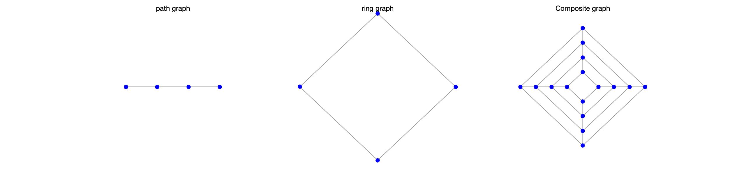
Fig. 1: Simulation graph: 4-note path graph, 4-note ring graph and 16-note composite graph.

We use two optimal sampling operators based on $\alpha=0.7,\beta=0.5$, the HGFRFT and HGFT to sample and interpolate the graph signal, and then use $\epsilon=||\mathbf{x}^{\prime}-\mathbf{x}||_{2}$ to measure the recovery accuracy. Fig. 2 shows the sampling coefficients. Fig. 3 (a) depicts the HGFRFT sampling, and (b) depicts the HGFT sampling. Fig. 4 (a) shows the signal perfectly recovered by sampling $(\epsilon=5.8055\times 10^{-17})$ by HGFRFT, while (b) shows the signal recovered by sampling $(\epsilon=0.8467)$ by HGFT. HGFT sampling cannot perfectly restore the graph signal because although the signal has a bandwidth limit of $\alpha=0.7,\beta=0.5$, the bandwidth in the generalized graph Fourier domain is not strictly limited. By Fig. 5 that when $\alpha=0.7$ is used during sampling, the error of the recovered signal is much smaller than when $\alpha$ takes other values. And when $\alpha=0.7$ and $\beta=0.5$, the error reaches the minimum value.

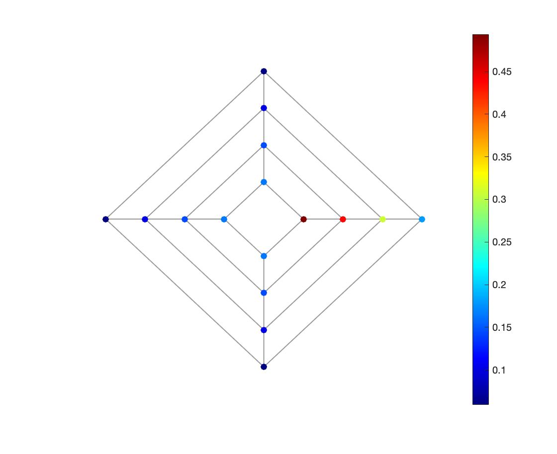
(a) Real part of 1st basis vector $\mathbf{f}_{1}$.

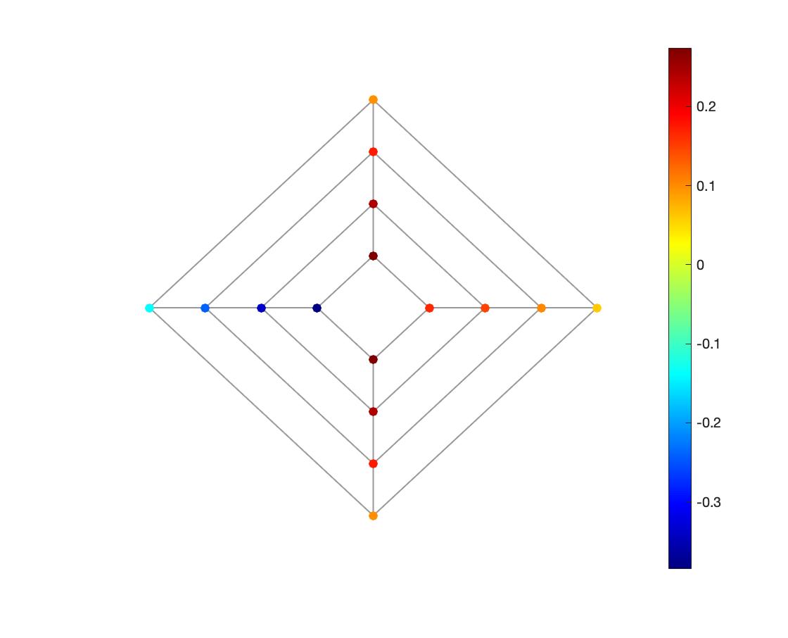
(b) Real part of 2nd basis vector $\mathbf{f}_{2}$.

(c) Real part of 3rd basis vector $\mathbf{f}_{3}$.

(d) Original graph signal.

Fig. 2: Graph signals on the composite graph.

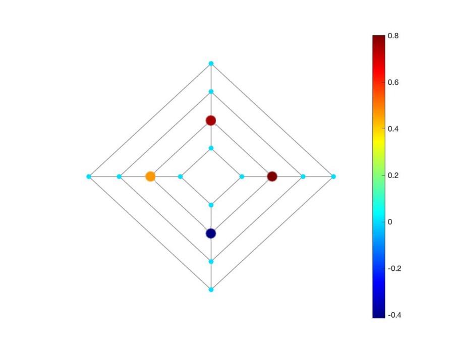
(a) Samples from HGFRFT sampling.

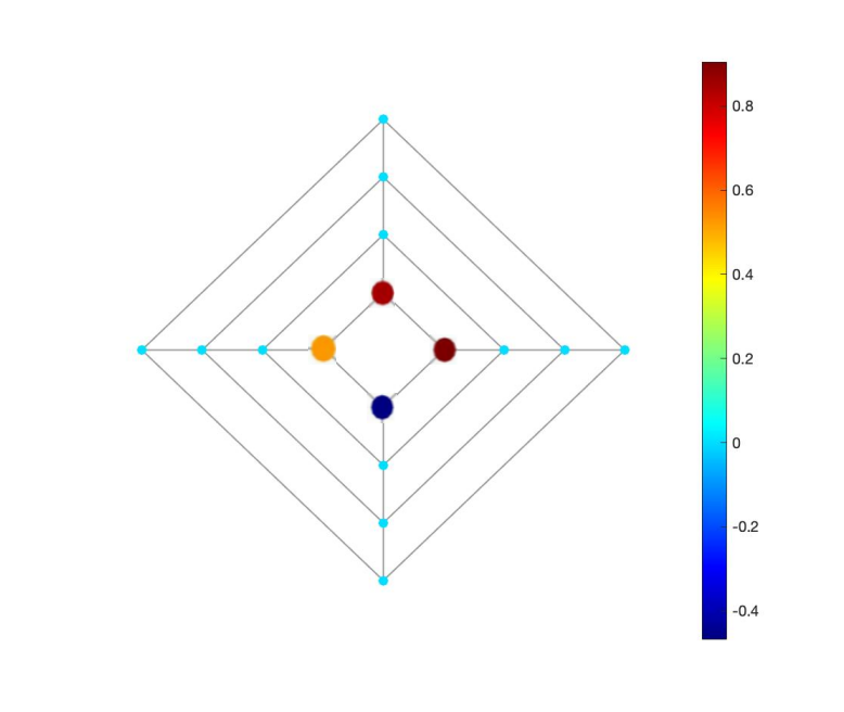
(b) Samples from HGFT sampling.

Fig. 3: Sampled signals. Large nodes represent the sampled nodes.

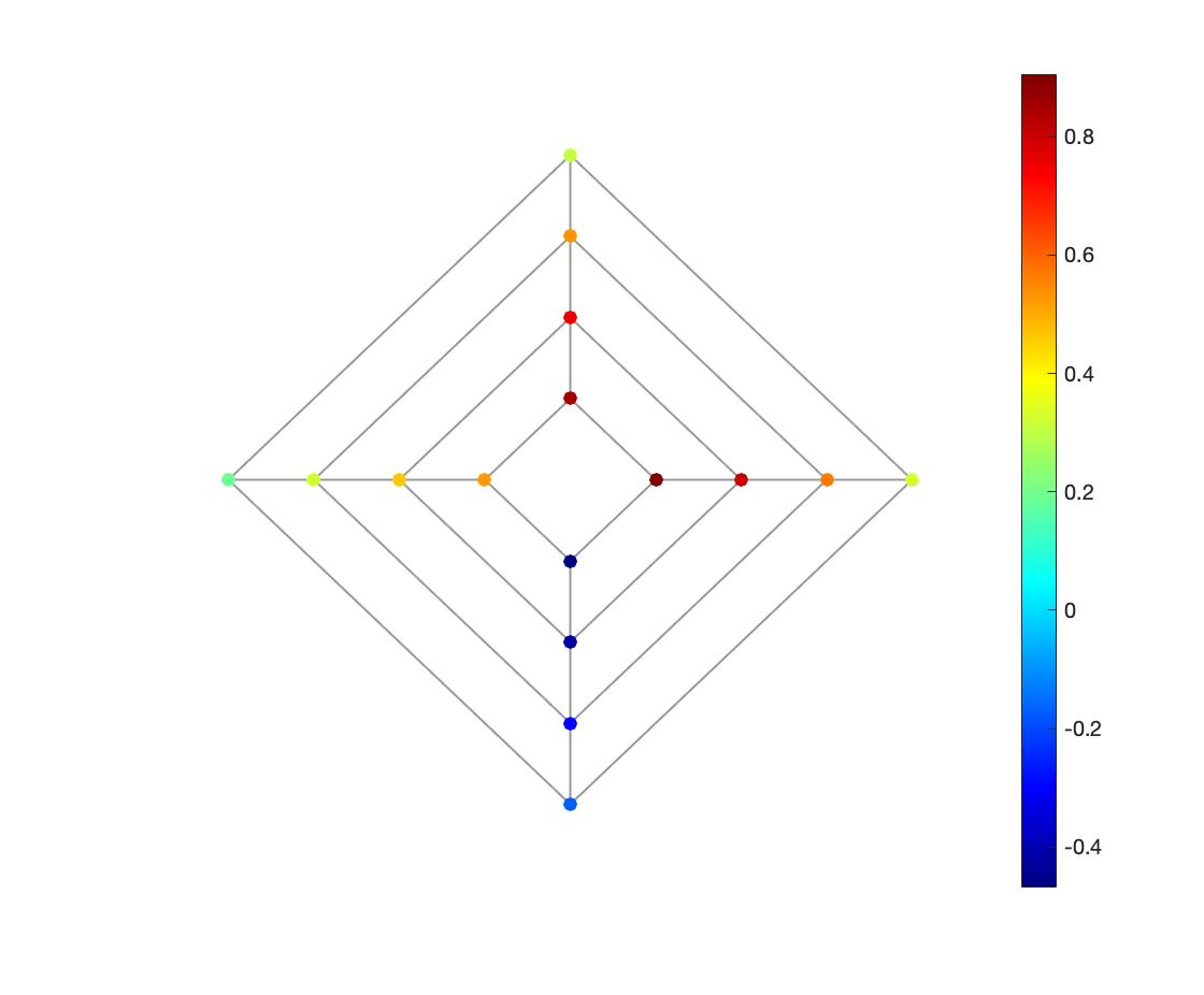
(a) Recovery from HGFRFT sampling.

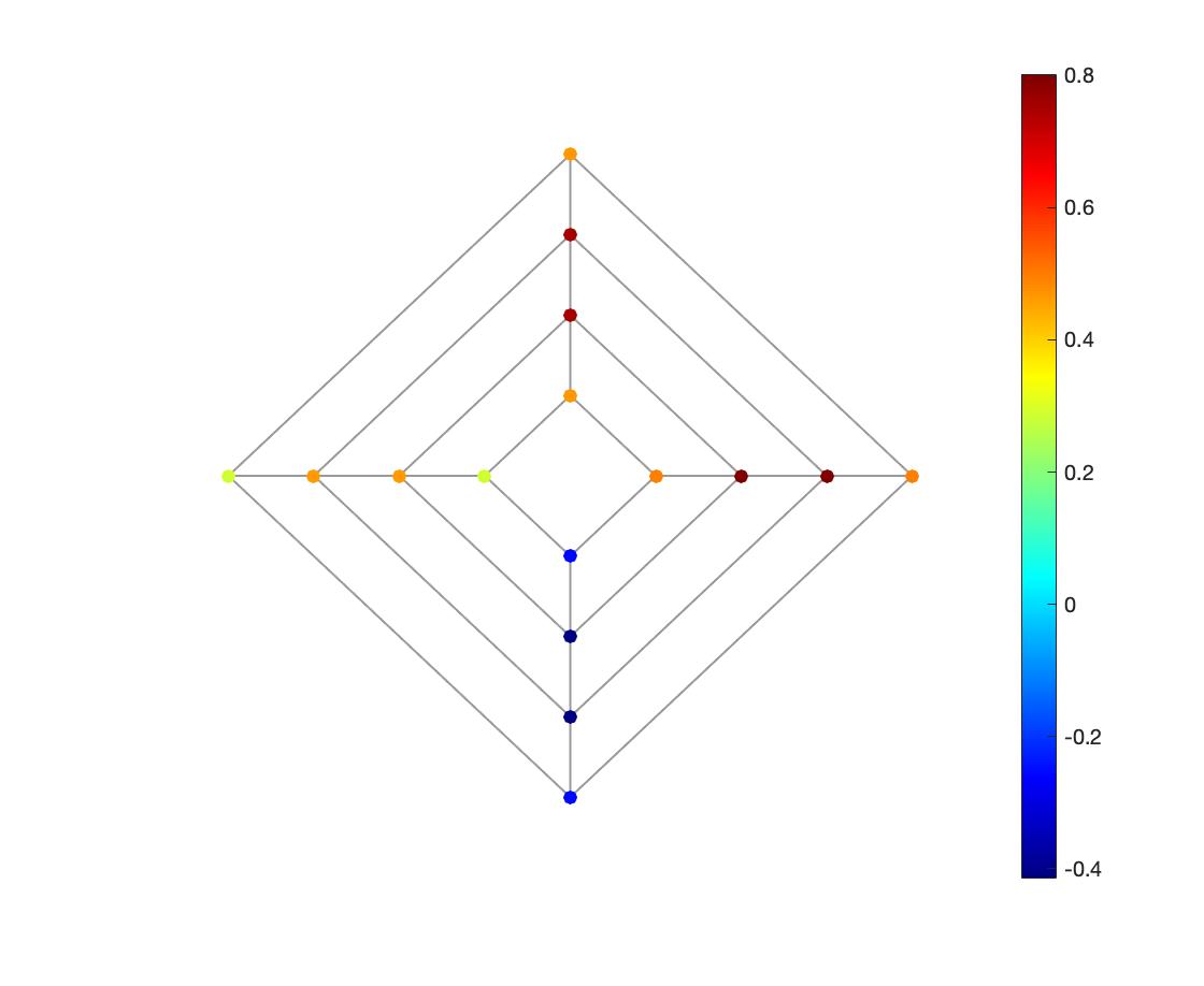
(b) Recovery from HGFT sampling.

Fig. 4: Recovered signals on the composite graph.

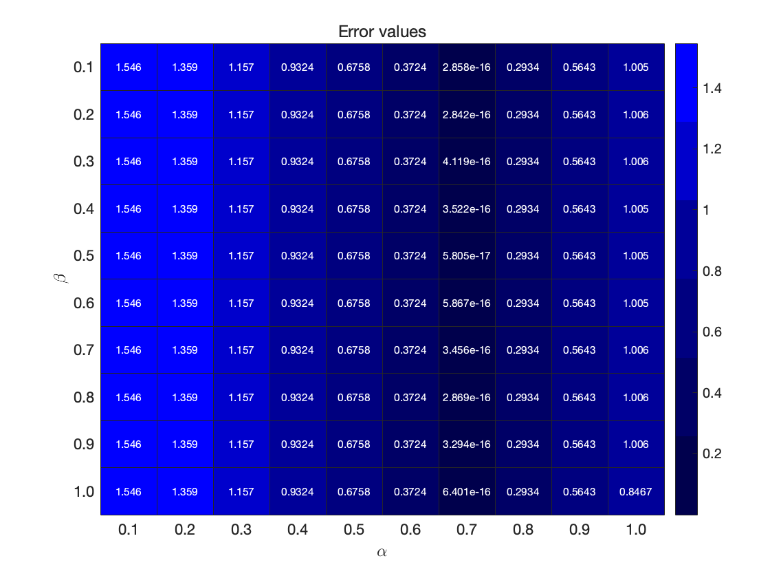
Fig. 5: Heat map of error values for different $\alpha$ and $\beta$.

VI-B Graph Frequency Analysis on Epidemic Models

In this part, we apply the HGFRFT to the complex dynamics of the network through the epidemic model [49], providing new methods and thinking for the evolution of nonlinear, discrete and nondeterministic models of infectious disease transmission.

Before the HGFRFT is performed, we first construct the graph, as shown in Fig. 6. Each node of the graph represents a city with a fixed population, and the edges of the graph are based on ground locations and airline connection graphs between major European cities.

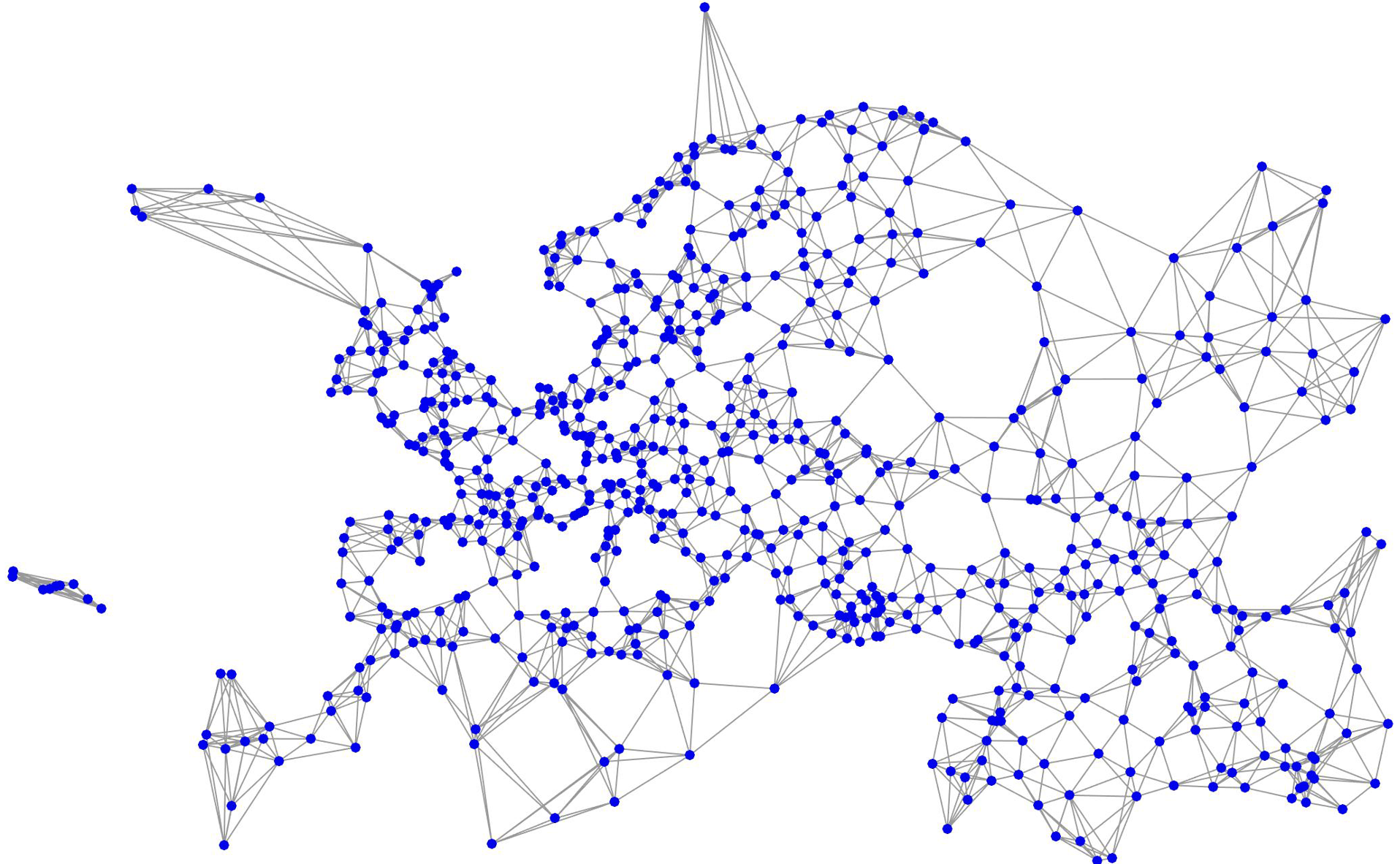
Fig. 6: Graph of some European cities.

An epidemic spread in N = 704 European cities is simulated according to two different compartmental models: the SEIR model and the SEIRS model. The model is parameterized with the infection’s contagion probability, infectious period, incubation period, and immune period.

Fig. 7 shows the HGFRFT for two different models simulating an epidemic outbreak. Each image shows the HGFRFT of the signal, depicting the evolution of the number of infections on the graph. The transformation is shown in the $(\omega,\lambda)$ plane, where a brighter color indicates a higher energy and $\alpha=0.93,\beta=0.95$.

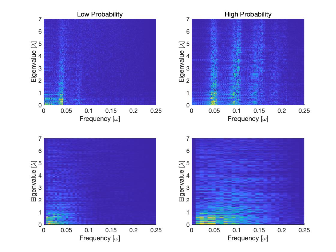
Fig. 7: The HGFRFT of the simulated epidemic breakouts for the two different models.

The HGFRFT can reveal that, for the SEIRS model, the spectrum is characterized by regularly spaced lines along the angular frequency axis, as each individual is likely to be reinfected after the temporary immunity period ends. In contrast, the SEIR model exhibits a more diffuse behavior without apparent periodicity. For each model, we can also use HGFRFT to distinguish between high and low infection probability scenarios.

VI-C Classifying Online Blogs

In this section, semisupervised classification is employed is to classify a large amount of data from a small number of labels; thus, the classification of online blogs is tested using fractional sampling and recovery in the Hilbert space, and the results are compared with those of HGFT sampling.

Data in a dataset with size $N=1224$ online political blogs are classified into $100$ groups of things as conservative or liberal [47]. Here, blogs and opinions on things compose as the composite graph, where we assign label signals 0 for conservatives and 1 for liberals. The constructed composite graph signal is shown in Fig. 8.

Fig. 8: Composite graph signal.

The labeled signal with the lowest fractional frequency components of $K$ is solved by the following optimization problem:

$$\hat{\mathbf{x}}^{opt}_{(K)}=\arg\min_{\hat{\mathbf{x}}_{(K)}\in\mathbb{R}^{K}}\left\|\mathrm{thres}\left(\Psi\mathbf{F}^{-\alpha,-\beta}_{(K)}\hat{\mathbf{x}}_{(K)}\right)-\mathbf{x}_{\mathcal{S}}\right\|^{2}_{2},$$ (38)

where the threshold function $\mathrm{thres}(\cdot)$ takes 0.5 as the threshold [50], the value greater than is specified as 1, and the value less than is specified as 0. In addition, set another threshold function with 0.5 as the threshold for the recovered signal,

$$\mathbf{x}^{opt}=\mathrm{thres}\left(\mathbf{F}^{-\alpha,-\beta}_{(K)}\hat{\mathbf{x}}^{opt}_{(K)}\right).$$ (39)

Fig. 9 (a) shows the change in classification accuracy by changing the fractional order $\alpha$ of the graph signal when we fix the fractional order $\beta=1$ and sample $S=K=2$ nodes in the Hilbert space, specifically $\alpha=1$ corresponding to HGFT sampling. When $\alpha=0.994$ and $0.995$, the accuracy rate reaches a maximum of 94.5261%, which is higher than the 94.1176% of HGFT. (b) shows that fractional sampling with order $\alpha=0.994$ yields a higher classification accuracy than HGFT sampling as $S$ varies.

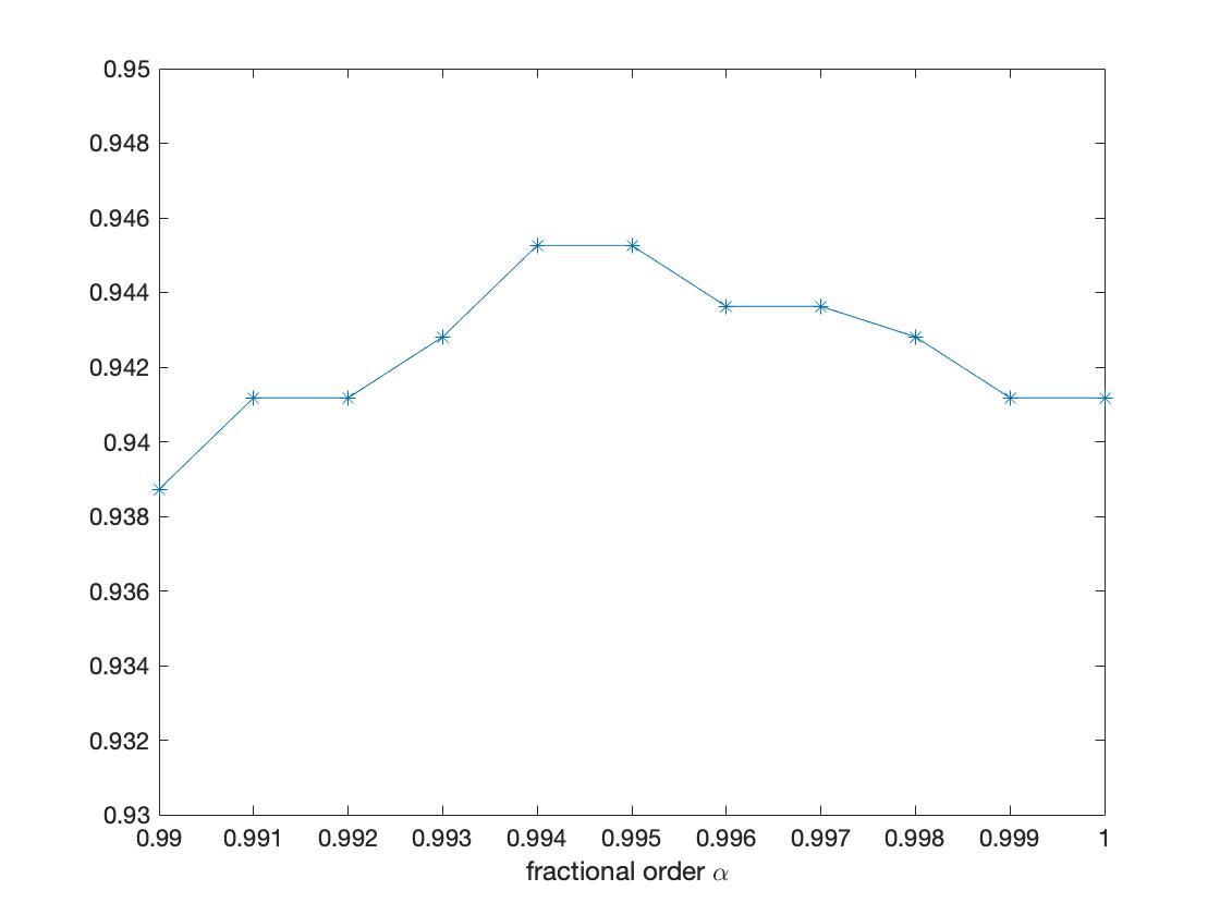
(a) Classification accuracy as a function of fractional order $\alpha$.

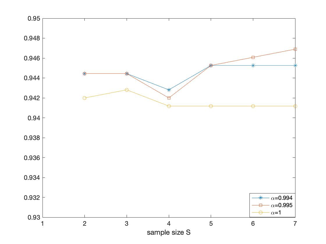
(b) Classification accuracy as a function of sample size $S$.

Fig. 9: Classification of online political blogs.

VI-D Comparison

To validate the quality of the HGFRFT when processing graph signals, energy compactness [16] can be used for comparison. The energy compactness of the DFRFT, the GFRFT and the HGFRFT in the dataset are calculated, as shown in Fig. 10. In Fig. 10, (a) is the dataset based on the number of infected people in Europe according to the SEIRS model, and (b) comprises the classified online blogs. It can be observed that the HGFRFT exhibits better energy compression properties in the dataset, especially for graphs under the Hilbert space, enabling it to effectively capture the signal structure and information.

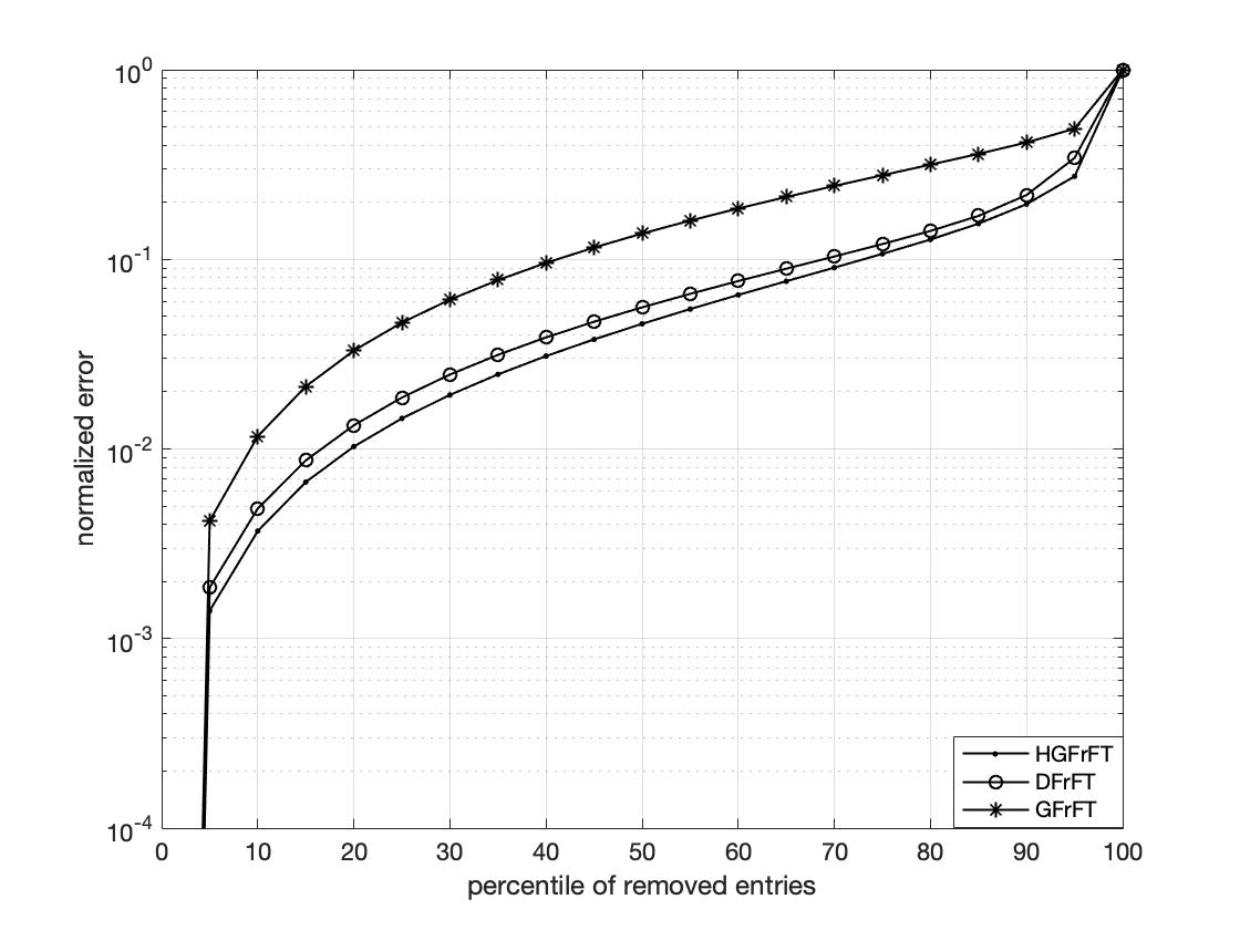
(a) The number of infected people.

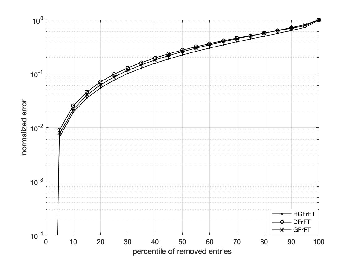
(b) The online blog classification.

Fig. 10: Compactness of different datasets.

VII Conclusion

In this paper, based on the concept of separable graph signals in Hilbert space, we propose the graph fractional Fourier transform (HGFRFT) of Hilbert space, which is a generalization of the Fourier transform of generalized GSP, just as the fractional Fourier transform (FRFT) generalizes the Fourier transform (FT). We also give some properties of HGFRFT. Furthermore, we propose a filtering and sampling theory for fractional domain signals, providing additional fractional analysis tools for the HGFRFT. These theories can be used to reduce signals in infinite continuous domains to more manageable finite domains. An example of a composite graph is given to illustrate the superiority of the HGFRFT. The framework extended in this paper and its corresponding theory are not only mathematically elegant but also practical. Some scenarios where the HGFRFT is applicable are also provided un the application and numerical experiments, but due to computational cost and space constraints, we only touch on some existing simple applications. In future work, we hope to be able to apply this framework to more complex real datasets and develop adaptability to different scenarios.

References

- [1] D. I. Shuman, S. K. Narang, P. Frossard, A. Ortega, and P. Vandergheynst, “The emerging field of signal processing on graphs: Extending high-dimensional data analysis to networks and other irregular domains,” IEEE Signal Process. Mag., vol. 30, no. 3, pp. 83-98, 2013.
- [2] A. Sandryhaila and J. M. F. Moura, “Big data processing with signal processing on graphs: Representation and processing of massive data sets with irregular structure,” IEEE Signal Process. Mag., vol. 31, no. 5, pp. 80-90, 2014.
- [3] A. Sandryhaila and J. M. F. Moura, “Discrete signal processing on graphs,” IEEE Trans. Signal Process., vol. 61, no. 7, pp. 1644-1656, 2013.
- [4] A. Ortega, P. Frossard, J. Kovačević, J. M. F. Moura, and P. Vandergheynst, “Graph signal processing: Overview, challenges, and applications,” Proc. IEEE, vol. 106, no. 5, pp. 808-828, 2018.
- [5] G. Leus, A. G. Marques, J. M. F. Moura, A. Ortega and D. I. Shuman, “Graph signal processing: History, development, impact, and outlook,” IEEE Signal Process. Mag., vol. 40, no. 4, pp. 49-60, 2023.
- [6] S. Chen, R. Varma, A. Sandryhaila, and J. Kovačević, “Discrete signal processing on graphs: Sampling theory,” IEEE Trans. Signal Process., vol. 63, no. 24, pp. 6510-6523, 2015.
- [7] A. Sakiyama, Y. Tanaka, T. Tanaka, and A. Ortega, “Eigendecomposition-free sampling set selection for graph signals,” IEEE Trans. Signal Process., vol. 67, no. 10, pp. 2679-2692, 2019.
- [8] J. Shi and J. M. F. Moura, “Graph signal processing: Dualizing GSP sampling in the vertex and spectral domains,” IEEE Trans. Signal Process., vol. 70, pp. 2883-2898, 2022.
- [9] M. W. Morency and G. Leus, “Graphon filters: Graph signal processing in the limit,” IEEE Trans. Signal Process., vol. 69, pp. 1740-1754, 2021.
- [10] A. Sandryhaila and J. M. F. Moura, “Discrete signal processing on graphs: Frequency analysis,” IEEE Trans. Signal Process., vol. 62, no. 12, pp. 3042-3054, 2014.
- [11] S. Chen, A. Sandryhaila, J. M. F. Moura, and J. Kovačević, “Signal recovery on graphs: Variation minimization,” IEEE Trans. Signal Process., vol. 63, no. 17, pp. 4609-4624, 2015.
- [12] A. Agaskar and Y. M. Lu, “A spectral graph uncertainty principle,” IEEE Trans. Inf. Theory, vol. 59, no. 7, pp. 4338–4356, 2013.
- [13] N. Perraudin, B. Ricaud, D. I. Shuman, and P. Vandergheynst, “Global and local uncertainty principles for signals on graphs,” APSIPA Trans. Signal Inf. Process., vol. 7, p. e3, 2018.
- [14] C. Cheng, Y. Chen, Y. J. Lee, and Q. Sun, “SVD-based graph Fourier transforms on directed product graphs,” IEEE Trans. Signal inf. Process. Netw., vol. 9, pp. 531-541, 2023.
- [15] D. I. Shuman, B. Ricaud, and P. Vandergheynst, “Vertex-frequency analysis on graphs,” Appl. Comput. Harmon. Anal., vol. 40, no. 2, pp. 260-291, 2016.
- [16] F. Grassi, A. Loukas, N. Perraudin, and B. Ricaud, “A time-vertex signal processing framework: Scalable processing and meaningful representations for time-series on graphs,” IEEE Trans. Signal Process., vol. 66, no. 3, pp. 817–829, 2018.
- [17] B. Kartal, E. Özgünay, and A. Koç, “Joint time-vertex fractional Fourier transform,” 2022, arXiv preprint, arXiv: 2203.07655.
- [18] B. Girault, A. Ortega, and S. S. Narayanan, “Irregularity-aware graph Fourier transforms,” IEEE Trans. Signal Process., vol. 66, no. 21, pp. 5746-5761, 2018.
- [19] N. Perraudin and P. Vandergheynst, “Stationary signal processing on graphs,” IEEE Trans. Signal Process., vol. 65, no. 13, pp. 3462–3477, 2017.
- [20] M. Belkin and P. Niyogi, “Semi-supervised learning on Riemannian manifolds,” Mach. Learn., vol. 56, no. 7, pp. 209–239, 2004.
- [21] M. Cheung, J. Shi, O. Wright, L. Y. Jiang, X. Liu, and J. M. F. Moura, “Graph signal processing and deep learning: Convolution, pooling, and topology,” IEEE Signal Process. Mag., vol. 37, no. 6, pp. 139–149, 2020.
- [22] M. Ye, V. Stankovic, L. Stankovic, and G. Cheung, “Robust deep graph based learning for binary classification,” IEEE Trans. Signal Inf. Process. Netw., vol. 7, pp. 322–335, 2021.
- [23] P. Lax, Functional analysis, 1st ed. Wiley-Interscience, 2002.
- [24] F. Ji and W. P. Tay, “A Hilbert space theory of generalized graph signal processing,” IEEE Trans. Signal Process., vol. 67, no. 24, pp. 6188-6203, 2019.
- [25] F. Ji and W. P. Tay, “Generalized graph signal processing,” in Proc. IEEE Global Conf. Signal Inf. Process. (GlobalSIP), 2018, pp. 708-712.
- [26] L. Yang, A. Qi, C. Huang, and J. Huang, “Graph Fourier transform based on norm variation minimization,” Appl. Comput. Harmon. Anal., vol. 52, pp. 348-365, 2021.
- [27] F. Ji, W. P. Tay, and A. Ortega, “Graph signal processing over a probability space of shift operators,” IEEE Trans. Signal Process., vol. 71, pp. 1159-1174, 2023.
- [28] Z. Ge, H. Guo, T. Wang, and Z. Yang, “The optimal joint time-vertex graph filter design: From ordinary graph Fourier domains to fractional graph Fourier domains,” Circuits, Syst. Signal Process., vol. 42, pp. 4002–4018, 2023.
- [29] F. Wang, G. Cheung, and Y. Wang, “Low-complexity graph sampling with noise and signal reconstruction via neumann series,” IEEE Trans. Signal Process., vol. 67, no. 21, pp. 5511-5526, 2019.
- [30] G. Ortiz-Jiménez, M. Coutino, S. P. Chepuri, and G. Leus, “Sampling and reconstruction of signals on product graphs,” in Proc. IEEE Global Conf. Signal Inf. Process. (GlobalSIP), 2018, pp. 713-717.
- [31] Z. Xiao, H. Fang, S. Tomasin, G. Mateos and X. Wang, “Joint sampling and reconstruction of time-varying signals over directed graphs,” IEEE Trans. Signal Process., vol. 71, pp. 2204-2219, 2023.
- [32] X. Jian and W. P. Tay, “Wide-sense stationarity and spectral estimation for generalized graph signal,” in Proc. IEEE Int. Conf. Acoust., Speech, Signal Process. (ICASSP), 2022, pp. 5827-5831.
- [33] V. Namias, “The fractional order Fourier transform and its application to quantum mechanics,” Ima J. Appl. Math., vol. 25, pp. 241-265, 1980.
- [34] L. B. Almeida, “The fractional Fourier transform and time-frequency representations,” IEEE Trans. Signal Process., vol. 42, no. 11, pp. 3084-3091, 1994.
- [35] Y. Q. Wang, B. Z. Li, and Q. Y. Cheng, “The fractional Fourier transform on graphs,” in Proc. Asia-Pacific Signal Inf. Process. Assoc. Annu. Summit Conf. (APSIPA ASC), 2017, pp. 105–110.
- [36] F. J. Yan and B. Z. Li, “Windowed fractional Fourier transform on graphs: Properties and fast algorithm,” Digit. Signal Process., vol. 118, 103210, 2021.
- [37] Y. Zhang and B. Z. Li, “Discrete linear canonical transform on graphs,” Digit. Signal Process., vol. 135, 103934, 2023.
- [38] Y. Q. Wang and B. Z. Li, “The fractional Fourier transform on graphs: Sampling and recovery,” in Proc. 14th IEEE Int. Conf. Signal Process. (ICSP), 2018, pp. 1103-1108.
- [39] C. Ozturk, H. M. Ozaktas, S. Gezici, and A. Koç, “Optimal fractional Fourier filtering for graph signals,” IEEE Trans. Signal Process., vol. 69, pp. 2902-2912, 2021.
- [40] F. J. Yan and B. Z. Li, “Spectral graph fractional Fourier transform for directed graphs and its application,” Signal Process., vol. 210, 109099, 2023.
- [41] L. Debnath and P. Mikusinski, Introduction to Hilbert spaces with applications, 3rd ed. burlington, MA: Elsevier Academic Press, 2005.
- [42] T. Hungerford, Algebra (graduate texts in mathematics) (v. 73), 8th ed. berlin, Germany: Springer, 2002.
- [43] J. Wu, F. Wu, Q. Yang, Y. Zhang, X. Liu, Y. Kong, L. Senhadji, and H. Shu, “Fractional spectral graph wavelets and their applications,” Math. Probl. Eng., 2020.
- [44] M. Puschel and J. M. F. Moura, “Algebraic signal processing theory: Foundation and 1-D time,” IEEE Trans. Signal Process., vol. 56, no. 8, pp. 3572-3585, 2008.
- [45] C. Shannon, “Communication in the presence of noise,” Proc. IRE, vol. 86, pp. 10-21, 1949.
- [46] J. Yu, X. Xie, H. Feng, and B. Hu, “On critical sampling of time-vertex graph signals,” in Proc. IEEE Global Conf. Signal Inf. Process. (GlobalSIP), 2019, pp. 1-5.
- [47] L. A. Adamic and N. Glance, “The political blogosphere and the 2004 U.S. election: divided they blog,” Proc. LinkKDD, pp. 35-43, 2005.
- [48] N. Perraudin, J. Paratte, D. Shuman, V. Kalofolias, P. Vandergheynst, and D. K. Hammond, “GSPBOX: a toolbox for signal processing on graphs,” 2016, arXiv preprint, arXiv: 1408.5781.
- [49] W. O. Kermack and A. G. McKendrick, “A contribution to the mathematical theory of epidemics,” Proc. Roy. Soc. London A, Math. Phys. Eng. Sci., vol. 115, no. 772, pp. 700–721, 1927.
- [50] C. M. Bishop, Pattern recognition and machine learning, information science and statistics, Springer, 2006.