Fractal Nambu Mechanics: Extending Dynamics with Fractal Calculus
Abstract
In this paper, we extend the principles of Nambu mechanics by incorporating fractal calculus. This extension introduces Hamiltonian and Lagrangian mechanics that incorporate fractal derivatives. By doing so, we broaden the scope of our analysis to encompass the dynamics of fractal systems, enabling us to capture their intricate and self-similar properties. This novel approach opens up new avenues for understanding and modeling complex fractal structures, thereby advancing our comprehension of these intricate phenomena.
1 Introduction
Fractal geometry explains shapes with self-similar properties that have fractional and complex numbers dimensions whose topological dimension is less than their fractal dimension [44, 39]. Fractals have different measures than Euclidean shapes. Fractals are seen in nature everywhere like clouds in the human body and the path of electrons and structures of materials in fractal forms show new results [8, 41]. Their properties have been studied with the help of mathematical analysis [22]. Fractals are explained in a mathematically rigorous manner, with an emphasis on examples and fundamental concepts such as Hausdorff dimension, self-similar sets, and Brownian motion [11]. Fractal structures are seen and used in many branches of physical science and art engineering [38, 10, 35, 34, 19, 21, 64]. Fractal space-time was considered in the different processes to obtain more general models to explain experimental data [51, 49, 67, 60]. Different techniques were used to analyze fractals, including probabilistic techniques, measure theory, fractional calculus, harmonic analysis, and fractional spaces [3, 65, 63, 58, 18, 14, 36, 68, 12, 15, 13, 25]. The -fractal function with variable parameters was investigated, focusing on the Weyl-Marchaud variable order fractional derivative under specific scaling factor conditions [56, 1, 2, 66]. The extension of Darcy’s law from conventional calculus to fractal calculus in order to quantify fluid flow in subterranean heterogeneous reservoirs was investigated [20, 57]
A generalization of Hamiltonian mechanics, Multi-Hamiltonian Nambu mechanics has some applications [47, 33, 32].
The flows created by a Hamiltonian over a Poisson manifold form the basis of Nambu mechanics. The trajectory in phase space is the intersection of the hypersurfaces specified by the invariants [47, 46]. The flow is perpendicular to all gradients of these Hamiltonians, parallel to the generalized cross product described by the corresponding Nambu bracket, and lagrangian to all gradients of these Hamiltonians. Nambu-Hamilton equations of motion, incorporating several Hamiltonians, describe the dynamics of Nambu mechanics. As a consistency condition, the basic identity for the Nambu bracket-which is comparable to the Jacobi identity-is presented [62, 16, 42].
The Hamiltonian embedding for Nambu’s novel mechanical equations is given. Using Dirac’s singular formalism, the embedding is investigated in both classical and quantization forms. The embedding Hamiltonian’s transformations are contrasted with Nambu’s canonical transformations [9, 24]. Nambu-Poisson and Nambu-Jacobi brackets are defined inductively [31]. In Nambu’s generalized mechanics, the action integral is defined on a world sheet and there is an additional degree of freedom in phase space
[40, 43]. The Nambu mechanics can, in theory, describe physical systems for which the Dirac mechanics is inappropriate since Nambu’s mechanics is independent of Dirac’s mechanics, at least in the odd instances [17]. The conditions for a Hamiltonian system to possess -linear Nambu brackets is investigated. The system should only have one degree of freedom for , but the criterion still holds for higher orders (). Levi-Civita tensors produce the canonical Nambu bracket, which is the only fundamental solution locally. [16]. A geometric formulation for a Hamiltonian system-like generalized form of Nambu mechanics is provided. It introduces a nondegenerate 3-form connected to a 3n-dimensional phase space to model temporal evolution. A Poisson bracket of two forms is additionally included, enabling the description of connected rigid bodies and non-integrable fluid flow [52]. Nambu mechanics is discussed using numerous instances of mechanical systems with the Nambu bracket. The relationship between a mechanical system’s superintegrability and the existence of the Nambu bracket is the main idea examined. The Nambu bracket’s uses in field theory are presented [59]. Using fractional-order differential forms and exterior derivatives, the creation of a fractional generalization of Nambu mechanics is shown. The generalized Pfaffian equations and offers a thorough analysis of one such example [5, 69, 26]. A fractal method to quantum chromodynamics is used to produce the Nambu-Jona-Lasino model, which includes a running coupling. Tsallis non-extensive statistical distributions in high-energy collisions are explained by the modified model [45].
The fractal analysis has been explored by multiple researchers through various approaches, including harmonic analysis [37], measure theory [23, 36, 25, 15, 12, 68], probabilistic methods [7], fractional space [61], fractional calculus [63, 30], and non-standard methods [48]. Through an expanded framework that contains differential equations, fractal calculus expands classical calculus. These equations’ solutions provide functions with fractal support, such as fractal sets and curves [55, 54, 53, 6, 27, 4].
The usage of fractal versions of Newton, Lagrange, Hamilton, and Appell’s mechanics is suggested. Following the definition of fractal velocity and acceleration, the Langevin equation on fractal curves is obtained. Hamilton’s mechanics on fractal curves are created via the Legendre transformation, allowing for the simulation of non-conservative systems with fractional dimensions [29].
Nonstandard analysis incorporating hyperreal and hyperinteger numbers is used to define left and right limits and derivatives on fractal curves. The use of nonstandard analysis is used to define the fractal integral and differential forms [28].
In this study, the generalization of Nambu mechanics is achieved by utilizing fractal derivatives and fractal differential forms on fractal manifolds. Through this approach, we extend the framework of Nambu mechanics to encompass fractal geometries and dynamics.
The following is the paper’s outline:
We present a concise summary of fractal calculus in Section 2, outlining its key concepts and principles. Moving on to Section 3, we introduce fractal Nambu mechanics, explaining its fundamental ideas and framework. In Section 4, we demonstrate the application of fractal differential forms in deriving Nambu mechanics. Additionally, in Section 6, we showcase the practical implementation and usefulness of this formalism through relevant examples and applications. Finally, in Section 7, we provide a comprehensive conclusion that summarizes the main findings and contributions of our work in the context of fractal Nambu mechanics.
2 Basic Tools
Definition 1.
The indicator function of is defined as
where .
Definition 2.
The coarse-grained measure of is defined as
| (1) |
where , and .
Definition 3.
The measure function of is defined as
Definition 4.
The fractal dimension of is defined as
Definition 5.
The integral staircase function of is defined as
where is a fixed number.
Definition 6.
For a function on an -perfect fractal set , the -derivative of at is defined as
if the fractal limit exists.
Definition 7.
The -integral of a bounded function , where (i.e., is a bounded function of ), is defined as
where , and the infimum or supremum is taken over all subdivisions .
Definition 8.
The fractal total derivative of a function can be defined when represent infinitesimal increments along the coordinate directions. It is denoted as and can be calculated as:
| (2) |
Here, or represents the fractal partial derivative of with respect to , and represents the infinitesimal increment in the -th coordinate direction [28].
3 Fractal Nambu mechanics
Nambu mechanics is a mathematical framework for explaining the dynamics of physical systems including several variables. Fractal Nambu mechanics is a modified form of Nambu mechanics. The idea of fractals is included in Fractal Nambu mechanics, enabling the characterization and study of complex systems with complicated and self-similar structures. The indicator function is used in Fractal Nambu mechanics to determine whether a fractal set is present or absent within a specified interval. The coarse-grained measure, which takes into account various scales of resolution, quantifies the size or extent of the fractal set within the interval. As the resolution becomes closer to zero, the measure function offers a limit that captures the fundamental characteristics of the fractal set. The complexity or self-similarity of the fractal set is gauged by the fractal dimension. The integral staircase function, which represents the total measure of the fractal set up to a specific point, is also introduced by Fractal Nambu mechanics. The fractal derivative and integral operators are defined using this function. The fractal integral computes the cumulative impact of a function on the fractal set, whereas the fractal derivative determines the rate of change of a function on the fractal set. Fractal Nambu mechanics, which incorporates fractal ideas into Nambu mechanics, offers a potent mathematical framework for investigating and comprehending complicated systems that exhibit fractal characteristics. It provides a deeper understanding of the dynamics and characteristics of such systems, allowing for a more thorough study and modeling strategy.
We present the mathematical framework of fractal Nambu mechanics as follows:
Definition 9.
A fractal manifold denoted as , characterized by fractal dimensions, is classified as a Fractal Nambu-Poisson manifold when a mapping denoted by
| (3) |
exists. Here, represents the space of smooth functions defined on fractal sets. This mapping can be referred to as the fractal Nambu-Poisson bracket of order , defined for any [55, 27].
The fractal Nambu-Poisson bracket exhibits specific properties, which include the following:
-
•
Skew-symmetry:
(4) Here, represents a permutation in the symmetric group , which consists of all possible arrangements of elements. The function determines the parity of the permutation, determining whether it is even or odd. The skew-symmetry property ensures that the resulting bracket remains consistent even when the functions’ order is altered, accounting for the sign change based on the parity of the permutation used.
-
•
Jacobi identity:
(5) The fractal Nambu-Poisson bracket obeys the Jacobi identity, which is a fundamental property of Poisson brackets. It states that the bracket of the bracket of functions with additional functions, along with the bracket of the first function with the bracket of the remaining functions, is equal to the bracket of the bracket of the first functions with the last functions.
-
•
Leibniz Rule:
(6) The fractal Nambu-Poisson bracket satisfies the Leibniz rule, also known as the generalized chain rule. This rule governs how the bracket operates on the product of functions, ensuring that the bracket operation can be applied to each function individually while preserving the appropriate sign and structure.
By satisfying these properties, the fractal Nambu-Poisson bracket of order provides a fundamental tool for describing the dynamics and relationships of smooth functions defined on Fractal Nambu-Poisson manifolds.
3.1 Fractal Nambu equations
In this subsection, the fractal Nambu equations are formulated using the fractal Nambu-Poisson bracket, as shown below:
| (7) | |||||
In this formulation, the local coordinates on the fractal Nambu-Poisson manifold are represented by , and the corresponding fractal Nambu-Hamiltonians are denoted as . The Levi-Civita tensor, denoted as , is involved in the equations.
It is important to note that while traditional Hamiltonian mechanics describes the state space using a pair of variables, and , Nambu mechanics extends this framework to include variables represented as .
Example 1.
Consider a triple dynamical variable that spans a three-dimensional phase space. Let and be Hamiltonians that determine the motion of points in the phase space. The fractal Nambu-Hamiltonians are given by the following equations
| (8) |
Alternatively, in vector notation, we have:
| (9) |
where
| (10) |
For any function , we have the following expression:
| (11) |
We can refer to the right-hand side of Eq. (1) as the fractal Nambu-Poisson bracket, denoted by . The orbit of the system in the fractal phase space is determined by the intersection of two surfaces, namely and . By using Eq. (9), we can write:
| (12) |
This may called the fractal Liouville theorem in the fractal Nambu phase space.
Definition 10.
By selecting an arbitrary as a generalized Hamiltonian, we can define as follows:
| (13) |
In this definition, satisfies the following conditions:
| (14) | ||||
| (15) |
Definition 11.
A mapping from to is considered a fractal canonical transform if it satisfies the condition:
| (16) |
Alternatively, it can be expressed as:
| (17) |
where and . In this definition, a fractal canonical transform refers to a mapping that preserves the fractal Nambu structure, ensuring that the fractal Nambu-Poisson brackets remain invariant under the transformation.
4 Fractal differential form and fractal Nambu mechanics
In this section, we introduce the concept of fractal differential forms to derive Nambu’s equations.
Definition 12.
The fractal Poincaré-Cartan 1-form is defined as follows:
| (18) |
Definition 13.
The fractal Poincaré-Cartan 2-form is defined as follows:
| (19) |
In these definitions, the variables , , and represent a triplet of dynamical variables, and and denote two Hamiltonians. The symbol represents the wedge product, a mathematical operation used in multivariable calculus. These fractal differential forms provide a mathematical framework for describing the dynamics and relationships between the variables involved in the Nambu system.
The Hamilton and Nambu equations can be derived by taking the exterior differentials of and , respectively. The resulting equations are as follows:
For :
| (20) |
This equation leads to Hamilton’s equations:
| (21) |
For :
| (22) |
This equation leads to the Nambu’s equations:
| (23) |
These equations describe the dynamics of the system in terms of the fractal derivatives and partial derivatives with respect to the variables involved. The Hamilton equations correspond to the case when and are the Hamiltonians, while the Nambu equations generalize the dynamics to more complex systems involving multiple variables and Hamiltonians.
5 Fractal Lagrangians in Nambu mechanics
We suggest a postulate that states the existence of Lagrangians matching to each Hamiltonian in order to achieve genuine Lagrangians in Nambu mechanics. We assume that the system contains an equal number of Lagrangians and Hamiltonians. Furthermore, we presume that each Lagrangian is consistent with the least action principle. In the most straightforward case, we suppose the presence of two Lagrangians, designated as and , which are equivalent to the system’s two Hamiltonians. With the help of this postulation, we can provide a thorough framework for figuring out the Lagrangians in Nambu mechanics [50].
| (24) |
Thus we have the two Euler-Lagrange equations for the two Lagrangians:
| (25) | ||||
| (26) |
Next, we define the first canonical momentum, denoted as , and the second canonical momentum, denoted as . The expressions for these momenta in terms of the Lagrangians are as follows:
| (27) | ||||
| (28) |
These momenta represent important quantities in Nambu mechanics, providing a measure of the conjugate momenta associated with the respective Lagrangians. Using Eq.(25) we have
| (29) | ||||
| (30) |
Now we define the two Hamiltonians and through fractal exterior differentials as follows:
| (31) |
where and are expressed in terms of , and . Then the left-hand side of Eq.(31) is equal
| (32) |
and the right-hand side of Eq.(31) is equal to, by virtue of Eqs. (27) and Eqs. (29) ,
| (33) |
Comparing Eqs.(5) and (5), we obtain Eq.(4) that establish the validity of our postulate regarding the existence of two Lagrangians and the corresponding definitions of the Hamiltonians.
6 Applications of Fractal Nambu Mechanics
In this section, we give some applications in classical mechanics.
Example 2.
Consider the Euler asymmetric top as an example. The Euler equation for this system can be derived as follows. Let’s define the following Hamiltonians:
| (34) |
where represent the inertia, and represent the components of the angular momenta. Using Eq.(1), we can obtain fractal Euler equations as:
| (35) |
Alternatively, we can express it as:
| (36) |
These equations describe the fractal Euler equations for the Euler asymmetric top system, where the fractal time derivatives of the angular momenta are expressed in terms of the inertia and the angular momenta themselves.
Example 3.
The fractal Nahm system, which serves as a model for static monopoles, can be obtained using fractal Nambu’s equation. Consider the Hamiltonians and where are constant. Applying fractal Nambu’s equation, we have:
| (37) |
Alternatively, we can express it as:
| (38) |
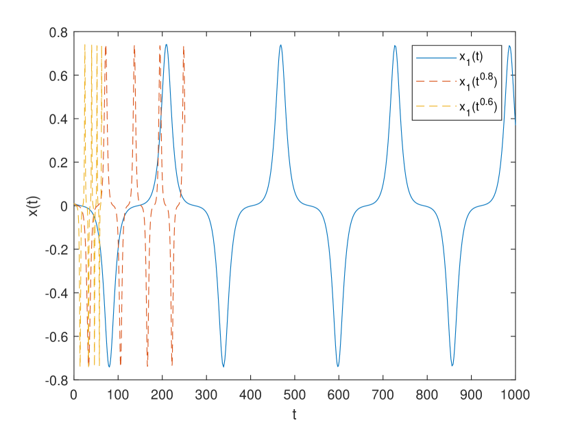
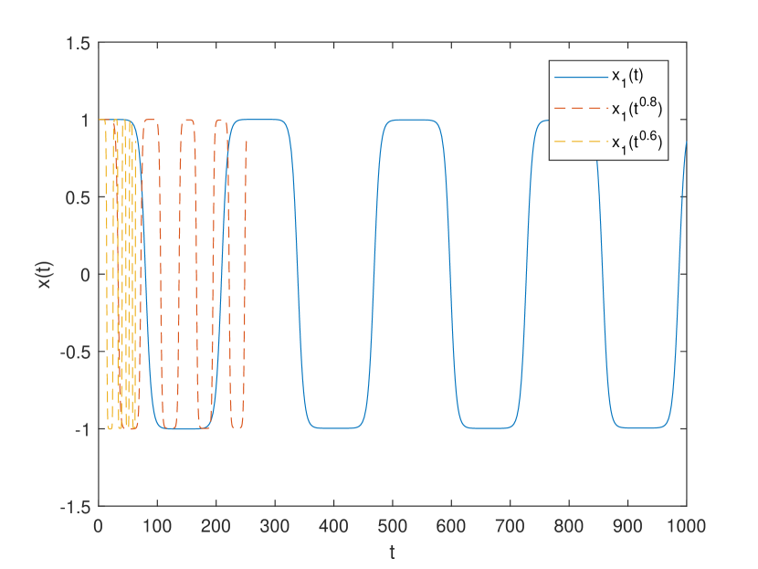
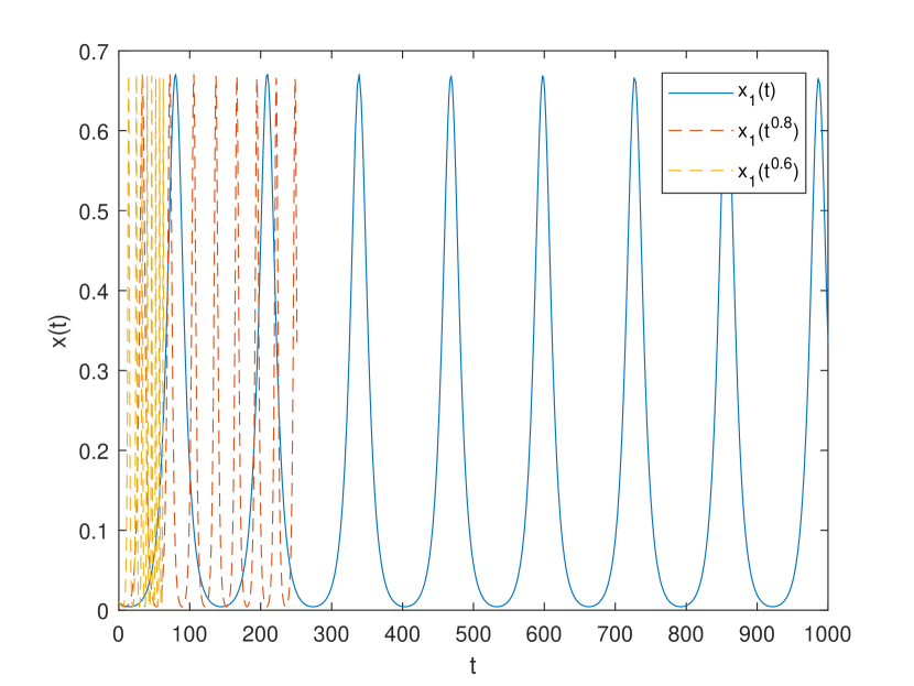
In Figures 1, 2, and 3, we showcase the solutions to Eq.(38). Here, we apply the condition with specific values assigned to the parameters, namely , , and .
These equations describe the fractal Nahm system, providing the time derivatives of the variables as products of the corresponding variables themselves. This model captures the dynamics of static monopoles.
Example 4.
Consider a 2-dimensional fractal harmonic oscillator described by the following Hamiltonians:
| (39) |
Here, , are constants. The corresponding fractal Nambu’s equation is given by:
| (40) |
In this equation, the curly brackets represent the fractal Nambu-Poisson bracket, and is an arbitrary function. The equation captures the dynamics of the system and highlights the interplay between the Hamiltonians and the additional function . The fractal Nambu’s equation provides a powerful tool for studying the behavior of the 2-dimensional fractal harmonic oscillator system.
7 Conclusion
In conclusion, Fractal Nambu mechanics is a mathematical framework that extends Nambu mechanics to incorporate fractal geometries and dynamics. Fractals, which are shapes with self-similar properties and fractional dimensions, are found in various natural and artificial systems. By utilizing fractal derivatives, fractal differential forms, and the fractal Nambu-Poisson bracket, Fractal Nambu mechanics provides a powerful tool for describing the dynamics of complex systems with fractal characteristics. The key features of Fractal Nambu mechanics include the formulation of fractal Nambu equations, which generalize the Hamilton and Nambu equations to systems with multiple variables and Hamiltonians. The fractal Nambu-Poisson bracket satisfies properties such as skew-symmetry, the Jacobi identity, and the Leibniz rule, ensuring consistency and preserving the Nambu structure. Fractal canonical transforms, which preserve the fractal Nambu structure, allow for the study of different coordinate systems. The introduction of fractal differential forms, such as the fractal Poincaré-Cartan 1-form and 2-form, enables the derivation of Nambu’s equations and provides a mathematical framework for describing the dynamics and relationships between variables in the Nambu system. Fractal Nambu mechanics finds applications in various areas of classical mechanics, allowing for the study of complex systems with fractal properties. Examples include the Euler asymmetric top, where the fractal Euler equations can be derived, and the study of dynamical systems in fractal phase spaces. Overall, Fractal Nambu mechanics provides a comprehensive and powerful framework for understanding and modeling complex systems with fractal characteristics, offering new insights and approaches to studying the dynamics of fractal structures.
References
- [1] A Agathiyan, A Gowrisankar, and Nur Aisyah Abdul Fataf. On the integral transform of fractal interpolation functions. Mathematics and Computers in Simulation, 2023.
- [2] A Agathiyan, A Gowrisankar, Nur Aisyah Abdul Fataf, and Jinde Cao. Remarks on the integral transform of non-linear fractal interpolation functions. Chaos, Solitons & Fractals, 173:113749, 2023.
- [3] Alexander S. Balankin. A continuum framework for mechanics of fractal materials i: from fractional space to continuum with fractal metric. Eur. Phys. J. B, 88(4), April 2015.
- [4] Alexander S Balankin and Baltasar Mena. Vector differential operators in a fractional dimensional space, on fractals, and in fractal continua. Chaos Solit. Fractals, 168:113203, 2023.
- [5] Dumitru Baleanu, Alireza K Golmankhaneh, and Ali K Golmankhaneh. Fractional nambu mechanics. International Journal of Theoretical Physics, 48:1044–1052, 2009.
- [6] Rawid Banchuin. Nonlocal fractal calculus based analyses of electrical circuits on fractal set. COMPEL - Int. J. Comput. Math. Electr. Electron. Eng., 41(1):528–549, 2022.
- [7] Martin T. Barlow and Edwin A. Perkins. Brownian motion on the sierpinski gasket. Probab. Theory Rel., 79(4):543–623, nov 1988.
- [8] Michael F Barnsley. Fractals Everywhere. Academic Press, New York, 2014.
- [9] F Bayen and M Flato. Remarks concerning nambu’s generalized mechanics. Physical Review D, 11(10):3049, 1975.
- [10] Luiz Bevilacqua and Marcelo M Barros. The inverse problem for fractal curves solved with the dynamical approach method. Chaos Solit. Fractals, 168:113113, 2023.
- [11] Christopher J Bishop and Yuval Peres. Fractals in probability and analysis, volume 162. Cambridge University Press, Cambridge, 2017.
- [12] D Bongiorno, G Corrao, et al. The Henstock-Kurzweil-Stieltjes type integral for real functions on a fractal subset of the real line. In Bollettino di Matematica pura e applicata vol. IV, volume 4, pages 5–16. Aracne, Boston, 2011.
- [13] Donatella Bongiorno. Derivatives not first return integrable on a fractal set. Ricerche di Matematica, 67(2):597–604, 2018.
- [14] Donatella Bongiorno. Derivation and integration on a fractal subset of the real line. In Dr. Sid-Ali Ouadfeul, editor, Fractal Analysis - Applications and Updates, chapter 7. IntechOpen, Rijeka, 2023.
- [15] Donatella Bongiorno and Giuseppa Corrao. On the fundamental theorem of calculus for fractal sets. Fractals, 23(02):1550008, 2015.
- [16] Cristel Chandre and Atsushi Horikoshi. Classical nambu brackets in higher dimensions. J. Math. Phys., 64(5), 2023.
- [17] Isaac Cohen and Andrés J Kálnay. On nambu’s generalized hamiltonian mechanics. International Journal of Theoretical Physics, 12:61–67, 1975.
- [18] M. Czachor. Waves along fractal coastlines: From fractal arithmetic to wave equations. Acta Phys. Pol. B, 50(4):813, 2019.
- [19] M Czachor. Contra bellum: Bell’s theorem as a confusion of languages. Acta Phys. Pol, 143(6):S158–S158, 2023.
- [20] Lucero Damián Adame, Claudia del Carmen Gutiérrez-Torres, Bernardo Figueroa-Espinoza, Juan Gabriel Barbosa-Saldaña, and José Alfredo Jiménez-Bernal. A mechanical picture of fractal darcy’s law. Fractal and Fractional, 7(9):639, 2023.
- [21] Airton Deppman and Eugenio Megías. Tsallis statistics and QCD thermodynamics. In EPJ Web of Conferences, volume 270, page 00033, 2022.
- [22] MS El Naschie. On certain infinite dimensional cantor sets and the schrödinger wave. Chaos Solit. Fractals, 3(1):89–98, 1993.
- [23] U Freiberg and Martina Zähle. Harmonic calculus on fractals-a measure geometric approach I. Potential Anal., 16(3):265–277, 2002.
- [24] Philippe Gautheron. Some remarks concerning nambu mechanics. Letters in Mathematical Physics, 37:103–116, 1996.
- [25] Massimiliano Giona. Fractal calculus on [0, 1]. Chaos Solit. Fractals, 5(6):987–1000, 1995.
- [26] Ali Khalili Golmankhaneh, AlirezaKhalili Golmankhaneh, Dumitru Baleanu, and Mihaela Cristina Baleanu. Fractional odd-dimensional mechanics. Adv. Differ. Equ., 2011:1–12, 2011.
- [27] Alireza Khalili Golmankhaneh. Fractal Calculus and its Applications. World Scientific, Singapore, 2022.
- [28] Alireza Khalili Golmankhaneh, Kerri Welch, Cristina Serpa, and Palle E T Jørgensen. Non-standard analysis for fractal calculus. The Journal of Analysis, 31:1895–1916, 2023.
- [29] Alireza Khalili Golmankhaneh, Kerri Welch, Cemil Tunç, and Yusif S Gasimov. Classical mechanics on fractal curves. Eur. Phys. J. Spec. Top., pages 1–9, 2023.
- [30] Arulprakash Gowrisankar, Alireza Khalili Golmankhaneh, and Cristina Serpa. Fractal calculus on fractal interpolation functions. Fractal Fract., 5(4):157, 2021.
- [31] Janusz Grabowski and Giuseppe Marmo. Remarks on nambu-poisson and nambu-jacobi brackets. J. Phys. A Math., 32(23):4239, 1999.
- [32] Partha Guha. Applications of nambu mechanics to systems of hydrodynamical type. J. Math. Phys., 43(8):4035–4040, 2002.
- [33] Partha Guha. Applications of nambu mechanics to systems of hydrodynamical type ii. J. Nonlinear Math. Phys., 11(2):223–232, 2004.
- [34] Ben Hambly and Peter Koepernik. Dimension results and local times for superdiffusions on fractals. Stoch. Process. their Appl., 158:377–417, 2023.
- [35] Yousef Heider, Franz Bamer, Firaz Ebrahem, and Bernd Markert. Self-organized criticality in fracture models at different scales. Examples and Counterexamples, 2:100054, 2022.
- [36] Huikun Jiang and Weiyi Su. Some fundamental results of calculus on fractal sets. Commun. Nonlinear Sci. Numer. Simul., 3(1):22–26, 1998.
- [37] Jun Kigami. Analysis on Fractals. Cambridge University Press, Cambridge, jun 2001.
- [38] MA Kotov, VM Volchuk, DM Zeziukov, and TM Pavlenko. Application of 3d fractal modeling for predicting concrete strength characteristics. In AIP Conference Proceedings, volume 2526. AIP Publishing, 2023.
- [39] Michel L. Lapidus, Goran Radunović, and Darko Žubrinić. Fractal Zeta Functions and Fractal Drums. Springer International Publishing, New York, 2017.
- [40] CC Lassig and Girish C Joshi. Constrained systems described by nambu mechanics. Lett. Math. Phys ., 41:59–63, 1997.
- [41] O. Linton. Fractals: On the Edge of Chaos. Wooden Books. Bloomsbury, New York, 2021.
- [42] Jaume Llibre, Rafael Ramírez, and Valentín Ramírez. Generalized Cartesian–Nambu vector fields. In Dynamics through First-Order Differential Equations in the Configuration Space, pages 177–283. Springer, New York, 2023.
- [43] Nugzar Makhaldiani. Nambu-poisson dynamics with some applications. arXiv preprint arXiv:1201.5105, 2011.
- [44] Benoit B Mandelbrot. The Fractal Geometry of Nature. WH freeman, New York, 1982.
- [45] E Megias, MJ Teixeira, VS Timóteo, and A Deppman. Nambu–jona-lasinio model with a fractal inspired coupling. arXiv preprint arXiv:2203.11080, 2022.
- [46] Yoichiro Nambu. On lagrangian and hamiltonian formalism. Progress of Theoretical Physics, 7(2):131–170, 1952.
- [47] Yoichiro Nambu. Generalized hamiltonian dynamics. Physical Review D, 7(8):2405, 1973.
- [48] L. Nottale and J. Schneider. Fractals and nonstandard analysis. J. Math. Phys., 25(5):1296–1300, may 1984.
- [49] Laurent Nottale. Fractal Space-Time and Microphysics: Towards a Theory of Scale Relativity. World Scientific, Singapore, 1993.
- [50] Tsuyoshi Ogawa and Toshiaki Sagae. Nambu mechanics in the lagrangian formalism. International Journal of Theoretical Physics, 39:2875–2890, 2000.
- [51] GN Ord. Fractal space-time: a geometric analogue of relativistic quantum mechanics. J. Phys. A Math., 16(9):1869, 1983.
- [52] Sagar A Pandit and Anil D Gangal. On generalized nambu mechanics. J. Phys. A Math., 31(12):2899, 1998.
- [53] A. Parvate and A.D. Gangal. Calculus on fractal subsets of real line-II: Conjugacy with ordinary calculus. Fractals, 19(03):271–290, sep 2011.
- [54] A. Parvate, S. Satin, and A.D. Gangal. Calculus on fractal curves in . Fractals, 19(01):15–27, mar 2011.
- [55] Abhay Parvate and Anil D Gangal. Calculus on fractal subsets of real line-I: Formulation. Fractals, 17(01):53–81, 2009.
- [56] TMC Priyanka, C Serpa, and A Gowrisankar. -fractal function with variable parameters: An explicit representation. Fractals, 2023.
- [57] Didier Samayoa, Ernesto Pineda León, Lucero Damián Adame, Eduardo Reyes de Luna, and Andriy Kryvko. The hausdorff dimension and capillary imbibition. Fractal and Fractional, 6(6):332, 2022.
- [58] Trifce. Sandev. Fractional Equations and Models: Theory and Applications. Springer, New York, 2020.
- [59] AO Shishanin. Nambu mechanics and its applications. In IOP Conference Series: Materials Science and Engineering, volume 468, page 012029. IOP Publishing, 2018.
- [60] M F Shlesinger. Fractal time in condensed matter. Annu. Rev. Phys. Chem., 39(1):269–290, oct 1988.
- [61] Frank H Stillinger. Axiomatic basis for spaces with noninteger dimension. J. Math. Phys., 18(6):1224–1234, 1977.
- [62] Leon Takhtajan. On foundation of the generalized nambu mechanics. Commun. Math. Phys., 160:295–315, 1994.
- [63] Vasily E. Tarasov. Fractional Dynamics. Springer Berlin Heidelberg, New York, 2010.
- [64] Walid Tarraf, Diogo Queiros-Condé, Patrick Ribeiro, and Rafik Absi. Fractal geometric model for statistical intermittency phenomenon. Entropy, 25(5):749, 2023.
- [65] Vladimir V Uchaikin. Fractional Derivatives for Physicists and Engineers, volume 2. Springer, New York, 2013.
- [66] R Valarmathi and A Gowrisankar. Variable order fractional calculus on -fractal functions. The Journal of Analysis, 31:2799–2815, 2023.
- [67] Susie Vrobel. Fractal Time. World Scientific, Singapore, jan 2011.
- [68] W.D. Withers. Fundamental theorems of calculus for hausdorff measures on the real line. J. Math. Anal. Appl., 129(2):581–595, feb 1988.
- [69] Yan-Li Xu and Shao-Kai Luo. Fractional nambu dynamics. Acta Mechanica, 226(11):3781–3793, 2015.