Frozen Feature Augmentation for Few-Shot Image Classification

Abstract

Training a linear classifier or lightweight model on top of pretrained vision model outputs, so-called ‘frozen features’, leads to impressive performance on a number of downstream few-shot tasks. Currently, frozen features are not modified during training. On the other hand, when networks are trained directly on images, data augmentation is a standard recipe that improves performance with no substantial overhead. In this paper, we conduct an extensive pilot study on few-shot image classification that explores applying data augmentations in the frozen feature space, dubbed ‘frozen feature augmentation (FroFA)’, covering twenty augmentations in total. Our study demonstrates that adopting a deceptively simple pointwise FroFA, such as brightness, can improve few-shot performance consistently across three network architectures, three large pretraining datasets, and eight transfer datasets.

1 Introduction

Vision transformers (ViTs) [19] achieve remarkable performance on ImageNet-sized [43, 67] and smaller [38, 41, 21] datasets. In this setup, data augmentation, i.e., a predefined set of stochastic input transformations, is a crucial ingredient. Examples for image augmentations are random cropping or pixel-wise modifications that change brightness or contrast. These are complemented by more advanced strategies [73, 13, 46], such as AutoAugment [12].

A more prevalent trend is to first pretrain vision models on large-scale datasets and then adapt them downstream [71, 6, 8, 49]. Notable, even training a simple linear classifier or lightweight model on top of ViT outputs, also known as frozen features, can yield remarkable performance across a number of diverse downstream few-shot tasks [52, 16, 25]. Given the success of image augmentations and frozen features, we ask: Can we effectively combine image augmentations and frozen features to train a lightweight model?

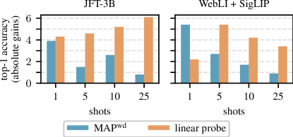
Figure 1: Average top-1 accuracy gains across seven few-shot test sets (CIFAR100 [1], SUN397 [69], …) on various few-shot settings. We train on frozen features from an L/16 ViT [19] with JFT-3B pretraining [71] or WebLI sigmoid language-image pretraining (SigLIP) [6, 72]. Our proposed frozen feature augmentation (FroFA) method gives consistent gains over a weight decay-regularized multi-head attention pooling [37] (MAP^wd) and an L2-regularized linear probe baseline, both without FroFA.

In this paper, we revisit standard image augmentation techniques and apply them on top of frozen features in a data-constrained, few-shot setting. We dub this type of augmentations frozen feature augmentations (FroFAs). Inspired directly by image augmentations, we first stochastically transform frozen features and then train a lightweight model on top. Our only modification before applying image augmentations on top of frozen features is a point-wise scaling such that each feature value lies in $[0,1]$ or $[0,255]$.

We investigate eight (few-shotted) image classification datasets using ViTs pretrained on JFT-3B [71], ImageNet-21k [17], or WebLI [6]. After extracting features from each few-shot dataset we apply twenty different frozen feature augmentations and train a lightweight multi-head attention pooling (MAP) [37] on top. Our major insights are:

1. Geometric augmentations that modify the shape and structure of two-dimensional frozen features always lead to worse performance on ILSVRC-2012 [57]. On the other hand, simple stylistic (point-wise) augmentations, such as brightness, contrast, and posterize, give steady improvements on 1-, 5-, and 10-shot settings.

2. Additional per-channel stochasticity by sampling independent values for each frozen feature channel works surprisingly well: On ILSVRC-2012 5-shot we improve over an MAP baseline by 1.6% absolute and exceed a well-tuned linear probe baseline by 0.8% absolute.

3. While FroFA provides modest but significant gains on ILSVRC-2012, it excels on seven smaller few-shot datasets. In particular, FroFA outperforms the mean 10-shot accuracy of an MAP baseline by 2.6% and the linear probe baseline by 5.2% absolute (cf. Fig. 1, left).

4. Results on the same seven few-shot datasets using a WebLI sigmoid language-image pretrained model [72] further emphasize the transfer capabilities of FroFA. We observe absolute gains ranging from 5.4% on 1-shot to 0.9% on 25-shot compared to an MAP baseline while outperforming a linear probe baseline by over 2% on 1-shot and at least 3% on 5- to 25-shot. (cf. Fig. 1, right).

2 Related Works

Few-shot transfer learning: State-of-the-art vision models [55, 32, 19, 71, 6, 16] are typically pretrained on large-scale datasets, e.g., ImageNet-21k [17] or JFT [27, 71], before transferred to other smaller-scale ones, e.g., CIFAR10 [1], SUN397 [68, 69], or ILSVRC-2012 [57]. Depending on the model size, efficient transfer learning becomes a challenge. Many methods have been proposed for large language models (LLMs), e.g., adapters [28], low-rank adaptation [29], or prompt tuning [39], of which some have been successfully adapted to computer vision [74, 5, 30, 22]. CLIP-Adapter [22] builds on contrastive language-image pretraining [52] and combines it with adapters [28]. A follow-up work [74] proposes TiP-Adapter which uses a query-key cache model [24, 51] instead of a gradient descent approach. Inspired by the success of prompt tuning in LLMs [39], Jia et al. propose visual prompt tuning at the model input [30]. On the other hand, AdaptFormer [5] uses additional intermediate trainable layers to finetune a frozen vision transformer [19].

In contrast, we do not introduce additional prompts [30] or intermediate parameters [22, 5] that require backpropagating through the network. Instead, we train a small network on top of frozen features from a ViT. This aligns with linear probing [52] which is typically used to transfer vision models to other tasks [25, 71, 16] — our objective.

Further, we focus on few-shot transfer learning [66, 36] in contrast to meta- or metric-based few-shot learning [59, 54, 2, 50, 48, 56, 9]. Kolesnikov et al. [32] and Dehghani et al. [16] reveal that a lightweight model trained on frozen features from a large-scale pretrained backbone yields high performance across a wide number of downstream (few-shot) tasks. Transfer learning has also shown to be competitive or slightly better than meta-learning approaches [20]. Building on these works, we propose frozen feature augmentation to improve few-shot transfer learning.

Data augmentation: One go-to method to improve performance while training in a low-data regime is data augmentation [60]. Some prominent candidates in computer vision are AutoAugment [12], AugMix [26], RandAugment [12], and TrivialAugment [46]. These methods typically combine low-level image augmentations together to augment the input. Works on augmentations in feature space exist [18, 65, 40, 44, 35], but lack a large-scale empirical study on frozen features of single-modal vision models.

To this end, we investigate frozen feature augmentation by reformulating twenty image augmentations, including a subset used in AutoAugment [12], inception crop [62], mixup [73, 65], and patch dropout [42].

3 Framework Overview

We introduce our notations in Sec. 3.1 followed by our caching and training pipeline in Sec. 3.2 and a description of frozen feature augmentations (FroFAs) in Sec. 3.3.

3.1 Notation

Let $\boldsymbol{x}\in\mathbb{I}^{H\times W\times 3}$ be an RGB image of height $H$, width $W$, and $\mathbb{I}=[0,1]$. A classification model processes $\boldsymbol{x}$ and outputs class scores $\boldsymbol{y}\in[0,1]^{S}$ for each class in a predefined set of classes $\mathcal{S}$, with $S=|\mathcal{S}|$. Let $L$ and $D$ be the number of intermediate layers and the number of features of a multi-layer classification model, respectively. We describe the intermediate feature representations of $\boldsymbol{x}$ as $\boldsymbol{f}=\boldsymbol{f}^{(\ell)}=(f^{(\ell)}_{d})\in\mathbb{R}^{D}$, with layer index $\ell\in\{1,...,L\}$ and feature index $d\in\{1,...,D\}$. In vision transformers [19], $\boldsymbol{f}=\boldsymbol{f}^{(\ell)}=(f^{(\ell)}_{n,c})\in\mathbb{R}^{N\times C}$ is typically two-dimensional, where $N$ and $C$ are the number of patches and number of per-patch channels, respectively. Finally, we introduce the patch index $n\in\{1,...,N\}$ and the per-patch channel index $c\in\{1,...,C\}$.

3.2 Training on Cached Frozen Features

We investigate pretrained vision transformers with $L$ transformer blocks (TBs) followed by a multi-head attention pooling (MAP) [37] and a classification layer (CL). Fig. 2(a) presents a simplified illustration. For simplicity, we neglect all operations before the first transformer block (e.g., patchifying, positional embedding, etc.).

To cache intermediate features, we process each image $\boldsymbol{x}$ from an image dataset $\mathcal{D}_{\boldsymbol{x}}$ through the network up until transformer block $L$. Next, we store the resulting features $\boldsymbol{f}$. After processing the entire image dataset $\mathcal{D}_{\boldsymbol{x}}$ we obtain a (frozen) feature dataset $\mathcal{D}_{\boldsymbol{f}}$, with $\boldsymbol{f}\in\mathcal{D}_{\boldsymbol{f}}$ (Fig. 2(b)).

Lastly, we train a lightweight model using the cached (frozen) features. Fig. 2(c) shows an example where a single MAP layer followed by a classification layer is trained using the feature dataset $\mathcal{D}_{\boldsymbol{f}}$. Since our focus is fast training, we defer a detailed analysis on larger models to future work.

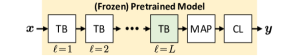
(a) Step 1: Select a (frozen) pretrained model and a layer for caching.

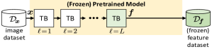
(b) Step 2: Process an image dataset and cache the (frozen) features.

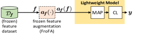
(c) Step 3: Train on (augmented) frozen features.

Figure 2: Pipeline for caching and training on (frozen) features. (2(a)): Given a (frozen) pretrained vision transformer, with $L$ transformer blocks (TBs), a multi-head attention pooling (MAP) layer, and a classification layer (CL), we select its $L$-th transformer block for caching. (2(b)): Next, we feed images $\boldsymbol{x}\in\mathcal{D}_{\boldsymbol{x}}$ to cache (frozen) features $\boldsymbol{f}\in\mathcal{D}_{\boldsymbol{f}}$. (2(c)): Finally, we use $\mathcal{D}_{\boldsymbol{f}}$ to train a lightweight model on top. We investigate frozen feature augmentation (FroFA) $\boldsymbol{a}_{\boldsymbol{f}}\in\mathcal{A}_{\boldsymbol{f}}$ in this scenario.

3.3 Frozen Feature Augmentation (FroFA)

Data augmentation is a common tool to improve generalization. However, it is typically applied on the input, or in our case: images. How can we map such image augmentations to intermediate transformer feature representations?

Recall that the feature representation $\boldsymbol{f}=(f_{n,c})\in\mathbb{R}^{N\times C}$ (layer index $\ell$ omitted) is two-dimensional. We first reshape it to a three-dimensional representation, i.e.,

$$\boldsymbol{f}^{*}=(f^{*}_{n_{1},n_{2},c})\in\mathbb{R}^{\sqrt{N}\times\sqrt{N}\times C}.$$ (1)

We further define

$$\boldsymbol{f}^{*}_{c}=\boldsymbol{f}^{*}_{:,:,c}\in\mathbb{R}^{\sqrt{N}\times\sqrt{N}\times 1}$$ (2)

as a reshaped two-dimensional representation of the $c$-th channel. Since images and features differ in two fundamental aspects, i.e., channel dimensionality and value range, we address this next.

Channel dimensionality: RGB images have just three channels while features can possess an arbitrary number of channels. To address this, we simply ignore image augmentations that rely on having three color channels, such as color jitter, and include only augmentations which can have an arbitrary number of channels instead, denoted as $C_{\boldsymbol{a}}$. This already covers a majority of commonly applied image augmentations.

Value range: RGB values lie within a specific range $\mathbb{I}$, e.g., $\mathbb{I}=[0,1]$ or $\mathbb{I}=\{0,...,255\}\subset\mathbb{N}_{0}$, while in theory features have no such constraints. Assuming $H=\sqrt{N}$ and $W=\sqrt{N}$, we define an image augmentation as

$$\boldsymbol{a}_{\boldsymbol{x}}:\mathbb{I}^{\sqrt{N}\times\sqrt{N}\times C_{\boldsymbol{a}}}\to\mathbb{I}^{\sqrt{N}\times\sqrt{N}\times C_{\boldsymbol{a}}},\boldsymbol{a}_{\boldsymbol{x}}\in\mathcal{A}_{\boldsymbol{x}},$$ (3)

where $\mathcal{A}_{\boldsymbol{x}}$ is the set of image augmentations. To also address the value range mismatch, we introduce a deterministic feature-to-image mapping

$$\boldsymbol{t}_{\boldsymbol{f}\rightarrow\boldsymbol{x}}:\mathbb{R}^{\sqrt{N}\times\sqrt{N}\times C_{\boldsymbol{t}}}\to\mathbb{I}^{\sqrt{N}\times\sqrt{N}\times C_{\boldsymbol{t}}}$$ (4)

that maps each element of $\boldsymbol{f}^{*}$ (1) from $\mathbb{R}$ to $\mathbb{I}$, with $C_{\boldsymbol{t}}$ as the number of channels of $\boldsymbol{f}^{*}$. We use

$$\boldsymbol{x}_{\boldsymbol{f}}=\boldsymbol{t}_{\boldsymbol{f}\rightarrow\boldsymbol{x}}(\boldsymbol{f}^{*})=\frac{\boldsymbol{f}^{*}-f_{\mathrm{min}}}{f_{\mathrm{max}}-f_{\mathrm{min}}},$$ (5)

where $f_{\mathrm{min}}$ and $f_{\mathrm{max}}$ are the minimum and maximum value of $\boldsymbol{f}^{*}$, respectively, with elements of $\boldsymbol{x}_{\boldsymbol{f}}$ now in $\mathbb{I}=[0,1]$. We further define an image-to-feature mapping

$$\boldsymbol{t}_{\boldsymbol{f}\leftarrow\boldsymbol{x}}:\mathbb{I}^{\sqrt{N}\times\sqrt{N}\times C_{\boldsymbol{t}}}\to\mathbb{R}^{\sqrt{N}\times\sqrt{N}\times C_{\boldsymbol{t}}}$$ (6)

that maps $\boldsymbol{x}_{\boldsymbol{f}}$ back to the original feature value range. In this case, we invert (4) and use

$$\boldsymbol{f}^{*}=\boldsymbol{t}_{\boldsymbol{f}\leftarrow\boldsymbol{x}}(\boldsymbol{x}_{\boldsymbol{f}})=\boldsymbol{x}_{\boldsymbol{f}}\cdot(f_{\mathrm{max}}-f_{\mathrm{min}})+f_{\mathrm{min}}.$$ (7)

Combining (3), (4), and (6), we obtain a generic (frozen) feature augmentation as a function composition

$$\boldsymbol{a}_{\boldsymbol{f}}=\boldsymbol{t}_{\boldsymbol{f}\leftarrow\boldsymbol{x}}\circ\boldsymbol{a}_{\boldsymbol{x}}\circ\boldsymbol{t}_{\boldsymbol{f}\rightarrow\boldsymbol{x}}.$$ (8)

We now define three variations of $\boldsymbol{a}_{\boldsymbol{f}}$:

1. (Default) FroFA: We apply $\boldsymbol{a}_{\boldsymbol{f}}$ (8) once across the entire feature. We set $C_{\boldsymbol{a}}=C_{\boldsymbol{t}}=C$ and compute $f_{\mathrm{min}}$ and $f_{\mathrm{max}}$ in (5), (7) across all elements of $\boldsymbol{f}^{*}$. Further, as normally done in pixel space, $\boldsymbol{a}_{\boldsymbol{x}}$ (3) samples a random augmentation value and changes all elements of $\boldsymbol{x}_{\boldsymbol{f}}$ using the same value. For example, employing random contrast in a FroFA fashion scales each element of $\boldsymbol{x}_{\boldsymbol{f}}$ by the exact same randomly sampled factor.

2. Channel FroFA (cFroFA): For each channel in the mapped features $\boldsymbol{x}_{\boldsymbol{f}}$ (5), $\boldsymbol{a}_{\boldsymbol{x}}$ (3) samples a random augmentation value per channel and applies that value to all elements in that channel ($C_{\boldsymbol{a}}=1$ while $C_{\boldsymbol{t}}=C$). By using cFroFA for our random contrast example, we obtain $C$ independently sampled scaling factors, one for each channel.

3. Channel² FroFA (c²FroFA): In addition to applying augmentations per channel ($C_{\boldsymbol{a}}=1$) as done in cFroFA, $\boldsymbol{t}_{\boldsymbol{f}\rightarrow\boldsymbol{x}}$ (4) and $\boldsymbol{t}_{\boldsymbol{x}\leftarrow\boldsymbol{f}}$ (6) also operate per channel ($C_{\boldsymbol{t}}=1$), i.e., on $\boldsymbol{f}^{*}_{c}$ (2). In this case, $f_{\mathrm{min}}$ and $f_{\mathrm{max}}$ are the per-channel maximum and minimum, respectively. In contrast, FroFA and cFroFA use the maximum and minimum across the entire feature. We denote this variant as c²FroFA since both the mappings (4), (6) and the augmentation (3) are applied on a per-channel basis. Although not adding additional stochasticity, we found that for random brightness this variant gives more stable results across a range of augmentation hyper parameters.

While an element-wise FroFA might seem like a natural next step, our initial experiments lead to significantly worse results. We hypothesize that per-element augmentations might lead to substantial changes in the feature appearance.

4 Experimental Setup

In this section, we describe our experimental setup.

4.1 Network Architectures

We employ pretrained Ti/16 [63], B/16 [19], and L/16 [19] vision transformers. Further, we follow Zhai et al. [71] and employ a lightweight multi-head attention pooling (MAP) [37] before the final classification layer for training on top of frozen features (cf. Sec. 3.3).

4.2 Datasets

Pretraining: We consider three pretraining datasets, i.e., JFT-3B [71], ImageNet-21k [17], and WebLI [6]. First introduced by Hinton et al. [27], JFT is now a widely used proprietary, large-scale dataset [10, 61, 32, 19, 14, 33, 6]. We use JFT-3B [71] which consists of nearly 3 billion multi-labeled images following a class-hierarchy of 29,593 labels. The images are annotated with noisy labels by using a semi-automated pipeline. We follow common practice [71, 16] and ignore the hierarchical aspect of the labels.

ImageNet-21k contains 14,197,122 (multi)-labeled images with 21,841 distinct labels. We equally split the first 51,200 images into a validation and test set and use the remaining 14,145,922 images for training.

Lastly, WebLI is a web-scale multilingual image-text dataset for vision-language training. It encompasses text in 109 languages with 10 billion images and roughly 31 billion image-text pairs.

Few-shot transfer learning: We investigate eight datasets for few-shot transfer learning, i.e., ILSVRC-2012 [57], CIFAR10 [1], CIFAR100 [1], DMLab [3, 70], DTD [11], Resisc45 [7], SUN397 [68, 69], and SVHN [47].

ILSVRC-2012, also known as ‘ImageNet-1k’ or just ‘ImageNet’, is a slimmed version of ImageNet-21k and contains 1,281,167 training images of 1,000 classes. We randomly sample 1-, 5-, 10-, and 25-shot versions from the first 10% of the training set. We further create additional disjoint sets by using the next four 10% fractions of the training set. In addition, we follow previous works [4] and create a ‘minival’ set using the last 1% (12,811 images) of the ILSVRC-2012 training set. The ‘minival’ set is used for hyperparameter tuning and design decisions while the official ILSVRC-2012 validation set is used as a test set. In summary, our setup consists of 1,000, 5,000, 10,000, or 25,000 training images, 12,811 validation images (‘minival’), and 50,000 test images (‘validation’).

For the other seven datasets, we select a training, validation, and test split for each dataset and create few-shot versions (1-, 5-, 10-, and 25-shot). Similar to ILSVRC-2012, we use the respective validation set to tune hyperparameters and report final results on the respective test set. A short description of each dataset and more details can be found in the Supplementary, Sec. S2.1.

4.3 Data Augmentation

We reuse the set of augmentations first defined in AutoAugment [12] and adopted in later works [13, 46]. In addition, we consider a few other image augmentations [62, 73, 42]. We select five geometric augmentations, i.e., rotate, shear-x, shear-y, translate-x, and translate-y; four crop & drop augmentations, i.e., crop, resized crop, inception crop [62], and patch dropout [42]; seven stylistic augmentations, i.e., brightness, contrast, equalize, invert, posterize, sharpness, and solarize; and two other augmentations, i.e., JPEG and mixup [73]. In Supplementary, Sec. S3.7, we also test two additional augmentations.

In total, we end up with twenty distinct augmentations. Note that all data augmentations incorporate random operations, e.g., a random shift in x- and y-direction (translate-x and translate-y, respectively), a randomly selected set of patches (patch dropout), a random additive value to each feature (brightness), or a random mix of two features and their respective classes (mixup). Please refer to the Supplementary, Sec. S2.2, for more details. We focus on the following set of experiments:

1. We investigate FroFA for all eighteen augmentations (and two additional ones in Supplementary, Sec. S3.7).

2. For our top-performing FroFAs, namely, brightness, contrast, and posterize, we incorporate additional stochasticity using cFroFA and c²FroFA (cf. Sec. 3.3).

3. We investigate a sequential protocol where two of the best three (c/c²)FroFA are arranged sequentially, namely, brightness c²FroFA, contrast FroFA, and posterize cFroFA. We test all six possible combinations.

4. Finally, we also apply variations of RandAugment [13] and TrivialAugment [46] directly on top of cached frozen features. More details and results can be found in the Supplementary, Secs. S2.2 and S3.2, respectively.

In Supplementary, Sec. S3.6, we complement our study by comparing our best FroFA to input data augmentations.

4.4 Training & Evaluation Details

We describe some base settings for pretraining, few-shot learning, and evaluation. Please refer to Supplementary, Sec. S2.3 for more training details.

Pretraining: Models are pretrained on Big Vision. We re-use the Ti/16, B/16, and L/16 ViTs pretrained on JFT-3B from Zhai et al. [71]. In addition, we pretrain Ti/16, B/16, and L/16 ViTs on ImageNet-21k following the settings described by Steiner et al. [60]. We further use a pretrained L/16 ViT image encoder stemming from a vision-language model from Zhai et al. [72] which follows their sigmoid language-image pretraining (SigLIP) on WebLI.

Few-shot transfer learning: Models are transferred using Scenic [15]. We train the lightweight MAP-based head by sweeping across five batch sizes (32, 64, 128, 256, and 512), four learning rates (0.01, 0.03, 0.06, and 0.1), and five training step sizes (1,000; 2000; 4,000; 8,000; and 16,000). In total, we obtain 100 configurations for each shot, but also investigate hyperparameter sensitivity on a smaller sweep in Supplementary, Sec. S3.5. For our experiments in Secs. 6 and 7, we also sweep four weight decay settings (0.01, 0.001, 0.0001, and 0.0, i.e., ‘no weight decay’), highlighted by a ‘wd’ superscript. We use the validation set for early stopping and to find the best setting across the sweep. Our cached-feature setup (cf. Fig. 2) fits on a single-host TPUv2 platform where our experiments run in the order of minutes.

Evaluation: We report the top-1 accuracy across all our few-shot datasets. Although we mainly report test performance, we tune all hyperparameters and base all of our design decisions on the validation set.

4.5 Baseline Models

We establish two baselines: MAP and linear probe.

MAP: We first cache the $N\!\times\!C$-shaped frozen features from the last transformer block. Afterwards, we train a lightweight MAP head (cf. Fig. 2) from scratch following the training protocol in Sec. 4.4. We add a ‘wd’ superscript, i.e., MAP^wd, whenever we include the weight decay sweep. For simplicity, the MAP head employs the same architectural design as the underlying pretrained model.

Linear probe: We use cached $1\!\times\!C$-shaped frozen features from the pretrained MAP head to solve an L2-regularized regression problem with a closed-form solution [71]. We sweep the L2 decay factor using exponents of 2 ranging from $-$20 up to 10. This setting is our auxiliary baseline.

5 Finding the Optimal FroFA Setup

We focus our first investigations on an L/16 ViT pretrained on JFT-3B, i.e., our largest model and largest pure image classification pretraining dataset, followed by few-shot transfer learning on subsets of the ILSVRC-2012 training set, i.e., our largest few-shot transfer dataset. We will refer to this setup as our JFT-3B L/16 base setup.

5.1 Baseline Performance

We first report the baseline performance in Tab. 1. We observe a large gap between MAP and linear probe on 1-shot ($-$8.6% absolute) which significantly decreases on 5-, 10-, and 25-shot settings to $-$0.8%, $-$0.6%, and $+$0.8% absolute, respectively.

In the following, our main point of comparison is the MAP baseline. This might be counter-intuitive since the performance is worse than linear probe in most cases. However, the higher input dimensionality in the MAP-based setting (cf. Sec. 4.5) gives us the option of input reshaping (cf. Sec. 3.3) which opens up more room and variety for frozen feature augmentations (FroFAs). Later in Sec. 6.3, we compare the performance of our best FroFA to the linear probe.

Baseline	1-shot	5-shot	10-shot	25-shot
MAP	57.9	78.8	80.9	83.2
Linear probe	66.5	79.6	81.5	82.4

Table 1: Baseline average top-1 accuracy on our ILSVRC-2012 test set. We use the JFT-3B L/16 base setup (cf. Sec. 5) and follow the respective baseline setting (cf. Sec. 4.5). Each shot is sampled five times. The best result per shot is boldfaced.

5.2 Default FroFA

			Geometric						Crop & drop					Stylistic								Other
Shots	MAP		rotate	shear-x	shear-y	translate-x	translate-y		crop	res. crop	incept. crop	patch drop.		brightness	contrast	equalize	invert	posterize	sharpness†	solarize†		JPEG†	mixup
1	57.9		$-$1.3	$-$0.6	$-$0.8	$-$1.2	$-$1.4		$+$3.0	$+$1.9	$+$0.0	$+$0.4		$+$4.8	$+$2.8	$+$1.0	$+$2.7	$+$3.7	$-$0.1	$+$1.0		$-$0.1	$-$1.4
5	78.8		$-$0.3	$-$0.2	$-$0.2	$-$0.3	$-$0.3		$+$0.0	$-$0.2	$+$0.0	$+$0.0		$+$1.1	$+$0.8	$+$0.5	$-$0.3	$+$0.8	$+$0.1	$-$0.1		$-$0.3	$-$0.3
10	80.9		$-$0.2	$-$0.1	$-$0.1	$-$0.2	$-$0.2		$+$0.0	$-$0.2	$+$0.0	$+$0.0		$+$0.6	$+$0.6	$+$0.4	$+$0.0	$+$0.6	$+$0.1	$+$0.0		$-$0.1	$+$0.2
25	83.2		$-$0.2	$-$0.1	$-$0.2	$-$0.1	$-$0.2		$+$0.0	$-$0.1	$-$0.1	$+$0.0		$+$0.1	$+$0.1	$+$0.0	$-$0.2	$+$0.0	$+$0.0	$+$0.0		$+$0.0	$+$0.1

Table 2: (Average) top-1 accuracy for default FroFA on our ILSVRC-2012 test set. Absolute gains to the MAP baseline are reported. We use the JFT-3B L/16 base setup (cf. Sec. 5). In total, we investigate eighteen FroFAs, categorized into geometric, crop & drop, stylistic, and other. We highlight deterioration by shades of red and improvement by shades of green. Each shot is sampled five times, except for augmentations marked with ‘$\dagger$’. Best three FroFAs are boldfaced.

We now investigate the effect of adding a single FroFA to the MAP baseline and start with the default FroFA formulation. Recall that we only use a single randomly sampled value per input (cf. Sec. 3.3). In Tab. 2, we report gains w.r.t. the MAP baseline on eighteen distinct FroFAs, categorized into geometric, crop & drop, stylistic, and other. In Supplementary, Sec. S3.7, we report on two additional FroFAs.

Geometric: Interestingly, all geometric augmentations consistently lead to worse performance across all settings.

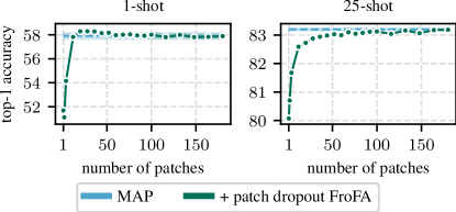
(a) Patch dropout FroFA

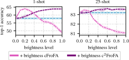
(b) Channel variants (c/c²) of brightness FroFA

Figure 3: Average top-1 accuracy for FroFA variants on our ILSVRC-2012 test set. We use the JFT-3B L/16 base setup (cf. Sec. 5). We sweep across a base sweep (cf. Sec. 4.4) to first find the best setting on our ILSVRC-2012 validation set for each FroFA operation point (cf. Supplementary, Sec. S2.2). Shaded areas indicate standard errors collected via sampling each shot five times.

Crop & drop: Applying a simple crop or a combination of resizing and crop yield a significant performance boost in the 1-shot setting of 3.0% and 1.9% absolute, respectively. Patch dropout, on the other hand, provides modest gains in the 1-shot regime. Dropping patches is directly related to training efficiency, so we investigate this further. Fig. 3(a) shows the top-1 accuracy on 1- and 25-shot as a function of number of patches. Results across other shots are similar (cf. Supplementary, Sec. S3.1). Similar to observations by Liu et al. [42] we can randomly drop a large fraction of patches ($>$50%) without loosing performance. A key difference is that Liu et al. only investigated the effect in the image space, while we provide evidence that patch dropout also transfers to the feature space. Finally, inception crop does not improve performance.

Stylistic: The largest gains can be observed when employing a stylistic FroFA, in particular brightness, contrast, and posterize. We identified brightness as the best performing FroFA with absolute gains of 4.8% on 1-shot, 1.1% on 5-shot, and up to 0.6% on 10-shot.

Other: Neither JPEG nor mixup yield performance gains but rather more or less worsen the performance.

5.3 Channel FroFA

			Brightness				Contrast			Posterize
Shots	MAP		-	c	c2		-	c		-	c
1	57.9		$+$4.8	$+$5.9	$+$6.1		$+$2.8	$+$2.5		$+$3.7	$+$5.9
5	78.8		$+$1.1	$+$1.5	$+$1.6		$+$0.8	$+$0.0		$+$0.8	$+$0.8
10	80.9		$+$0.6	$+$1.1	$+$0.9		$+$0.6	$+$0.0		$+$0.6	$+$0.5
25	83.2		$+$0.1	$+$0.4	$+$0.3		$+$0.1	$-$0.1		$+$0.0	$+$0.0

Table 3: Average top-1 accuracy for a selection of default (-) and channel (c/c²) FroFA on our ILSVRC-2012 test set. Absolute gains to the MAP baseline are reported. We use the JFT-3B L/16 base setup (cf. Sec. 5). Each shot is sampled five times. The best results per shot and FroFA are boldfaced (multiple ones if close, i.e., $\pm$0.2).

We continue with channel FroFA (cFroFA) using three stylistic augmentations: brightness, contrast, and posterize. In Tab. 3, we report absolute gains w.r.t. the MAP baseline and incorporate channel (c) and non-channel (-) variants. First, contrast cFroFA does not improve upon its non-channel variant across all shots. Second, posterize cFroFA improves performance on 1-shot from 3.7% to 5.9% while maintaining performance on all other shots. Lastly, brightness cFroFA significantly improves performance across all shots: 4.8% $\rightarrow$ 5.9% on 1-shot, 1.1% $\rightarrow$ 1.5% on 5-shot, 0.6% $\rightarrow$ 1.1% on 10-shot, and 0.1% $\rightarrow$ 0.4% on 25-shot.

Given the strong improvements for brightness cFroFA, we further test brightness c²FroFA (c² in Tab. 3). On a first look, the c²FroFA variant performs comparable to the cFroFA variant. In Fig. 3(b), we report top-1 accuracy on 1- and 25-shot as a function of the brightness level. Results across other shots are similar and can be found in Supplementary, Sec. S3.1. Now we clearly observe that brightness cFroFA is more sensitive to the brightness level than brightness c²FroFA. In general, brightness cFroFA only works well for small brightness levels (0.1 to 0.5), while its c²FroFA counterpart performs better than the MAP baseline across the board. We attribute the better sensitivity properties of brightness c²FroFA to the channel-wise mappings (5), (7) on $\boldsymbol{f}^{*}_{c}$ (2) since this is the only change compared to cFroFA. We did not observe similar effects for posterize when switching from cFroFA to c²FroFA.

5.4 Sequential FroFA

Finally, out of our best three augmentations, i.e., brightness c²FroFA (Bc²), contrast FroFA (C), and posterize cFroFA (Pc), we combine two of them sequentially ($\rightarrow$) yielding six combinations. In Tab. 4, we compare all six combinations to our prior best (Bc²). On 1-shot, ‘Bc²$\rightarrow$Pc’ significantly outperforms ‘Bc²’, improving absolute gains from 6.1% to 7.7%, while maintaining performance on other shots. We conclude that advanced FroFA protocols may further improve performance. As an initial investigation, we applied variations of RandAugment and TrivialAugment using our best three FroFAs (cf. Tab. 3), however, with limited success. We include results in the Supplementary, Sec. S3.2, and leave a deeper investigation to future works.

6 Results on More Model Architectures and Pretraining Datasets

How well does our best non-sequential FroFA strategy, i.e., brightness c²FroFA, transfer across multiple architecture and pretraining setups? We address this question in Secs. 6.1 and 6.2 and explore FroFA on ILSVRC-2012 frozen features from Ti/16, B/16, and L/16 ViTs pretrained on JFT-3B or ImageNet-21k, respectively. We further provide a comparison to linear probe in Sec. 6.3. Throughout this section, we report results on ILSVRC-2012. Further, in this section and Sec. 7, all MAP-based models employ a weight decay sweep denoted as MAP^wd (Sec. 4.4).

6.1 JFT-3B Pretraining

In Fig. 4(a), we report improvements in top-1 accuracy w.r.t. the MAP^wd baseline for Ti/16, B/16, and L/16 ViTs pretrained on JFT-3B. Across all shots and all architectures incorporating FroFA either maintains or improves performance over the MAP^wd baseline. On 1-shot, we further observe increasing improvements from FroFA on scaling the architecture. With higher shots, the improvement over the baseline becomes smaller. We attribute this to the already strong baseline performance leaving lesser headroom for improvements. We refer to the Supplementary, Sec. S3.3, for the exact values.

Shots	MAP		Bc2		Bc2$\rightarrow$C	C$\rightarrow$ Bc2		Bc2$\rightarrow$Pc	Pc$\rightarrow$ Bc2		C$\rightarrow$Pc	Pc$\rightarrow$C
1	57.9		$+$6.1		$+$4.0	$+$2.7		$+$7.7	$+$5.2		$+$5.0	$+$3.1
5	78.8		$+$1.6		$+$1.5	$+$0.2		$+$1.5	$+$0.4		$+$1.3	$+$0.0
10	80.9		$+$0.9		$+$1.2	$+$0.1		$+$1.0	$+$0.1		$+$0.9	$+$0.3
25	83.2		$+$0.3		$+$0.4	$-$0.7		$+$0.2	$-$0.5		$+$0.2	$-$0.4

Table 4: Average top-1 accuracy for a sequential FroFA protocol on our ILSVRC-2012 test set. Absolute gains to the MAP baseline are reported. We use the JFT-3B L/16 base setup (cf. Sec. 5). We combine the best settings of brightness c²FroFA (Bc²), contrast FroFA (C), and posterize cFroFA (Pc) sequentially (two at a time, order indicated by ‘$\uparrow$’). Each shot is sampled five times. The best results per shot are boldfaced (multiple ones if close, i.e., $\pm$0.2).

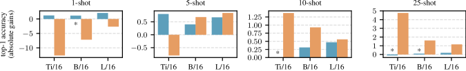
(a) JFT-3B

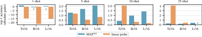
(b) ImageNet21k

Figure 4: Average top-1 accuracy of brightness c²FroFA combined with weight decay for JFT-3B 4(a) and ImageNet-21k 4(b) ViTs on our ILSVRC-2012 test set trained on few-shotted ILSVRC-2012 training sets. Absolute gains to the weight-decayed MAP, i.e. MAP^wd, and L2-regularized linear probe baseline are reported. Each shot is sampled five times. An asterisk (*) indicates that statistical significance is not given under a two-tailed t-test with 95% confidence for that particular ‘pretraining, shots, model, baseline’-setting (e.g., ‘JFT3-B, 10-shot, Ti/16, MAP’ or ‘ImageNet-21k, 25-shot, L/16, linear probe’).

6.2 ImageNet-21k Pretraining

In Fig. 4(b), we again look at improvements in top-1 accuracy w.r.t. the MAP^wd baseline for the same ViTs, but now pretrained on ImageNet-21k. Consistent with our JFT-3B results, the performance either maintains or improves over the MAP^wd baseline by incorporating FroFA and the improvements over the baseline become smaller with higher shots. We further observe increasing improvements from FroFA on scaling the architecture on 5- and 10-shot. We refer to the Supplementary, Sec. S3.3, for the exact values.

6.3 Linear Probe Comparison

Finally, we revisit Figs. 4(a) and 4(b), but now discuss gains w.r.t. the linear probe baseline. We start with models pretrained on JFT-3B (cf. Fig. 4(a)). On 1-shot, we observe that we lack behind linear probe but can close the gap by scaling up the model size. On 5- to 25-shot, with the exception of Ti/16 on 5-shot, brightness c²FroFA significantly outperforms the linear probe baseline. On ImageNet-21k (cf. Fig. 4(b)), we observe even larger gaps to linear probe on 1-shot (up to $-$20% absolute). However, similar to results on JFT-3B, performance on 5- to 25-shot improves significantly over linear probe or at worst stays the same.

7 Results on More Few-Shot Datasets and Vision-Language Pretraining

Our study so far explored FroFA on ILSVRC-2012 as a few-shot dataset. In this section, we analyze FroFA on seven additional few-shot datasets, i.e., CIFAR10, CIFAR100, DMLab, DTD, Resisc45, SUN397, and SVHN. In Sec. 7.1, we first use an L/16 ViT pretrained on JFT-3B for our analysis. In Sec. 7.2, we extend this analysis with the L/16 ViT image encoder of a vision-language model which was pretrained with sigmoid language-image pretraining (SigLIP) [72] on WebLI.

Pretraining scheme	Method	1-shot	5-shot	10-shot	25-shot
JFT-3B	MAPwd	49.5	65.8	68.3	74.1
	Linear probe	49.1	62.7	65.7	68.8
	MAPwd + FroFA	53.4	67.3	70.9	74.9
WebLI + SigLIP	MAPwd	45.9	67.7	71.8	75.1
	Linear probe	49.1	65.0	69.3	72.6
	MAPwd + FroFA	51.3	70.4	73.5	76.0

Table 5: Average top-1 accuracy of our best FroFA computed across seven few-shot datasets using a JFT-3B or WebLI-SigLIP L/16 ViT with weight decay. We report the mean across all test sets and refer to Supplementary, Tabs. 11 and 12, for more details. Per shot and dataset, the best result is boldfaced.

7.1 JFT-3B Pretraining

In Tab. 5 (upper half), we report mean results over the seven few-shot datasets using a JFT-3B L/16 ViT. Per dataset and shot, top-1 accuracy and two-tailed t-tests with 95% confidence are provided in Supplementary, Tab. 11. We compare the MAP^wd and linear probe baseline with MAP^wd combined with brightness c²FroFA (MAP^wd + FroFA). Across all shots, ‘MAP^wd + FroFA’ yields the highest mean results, surpassing the second-best approach (MAP^wd) by 3.9%, 1.5%, 2.6%, and 0.8% absolute on 1-, 5-, 10-, and 25-shot, respectively (cf. Fig. 1, left). Furthermore, Fig. 1 (left) reveals that while the gains to MAP^wd diminish with higher shots, the gains to linear probe actually increase and amount to at least 4.0% absolute across all shots.

7.2 WebLI Vision-Language Pretraining

Given the strong performance with the JFT-3B L/16 ViT, we finally ask: Does FroFA also transfer to ViTs with vision-language pretraining?

To answer this question, we train ‘MAP^wd’, ‘linear probe’, and ‘MAP^wd + FroFA’ using frozen features from the L/16 ViT image encoder of a WebLI-SigLIP vision-language model. In Tab. 5 (lower half), we report mean results over the same seven few-shot datasets from before. We again provide more detailed results and two-tailed t-tests in Supplementary, Tab. 12. Across all shots, ‘MAP^wd + FroFA’ again yields the highest mean results, surpassing the second-best approach on 1-shot (linear probe) by 2.2% absolute and the second-best approach on 5-, 10-, and 25-shot (MAP^wd) by 2.7%, 1.7%, and 0.9% absolute, respectively (cf. Fig. 1, right). In Fig. 1 (right), we observe that the gains to both MAP^wd and linear probe (neglecting 1-shot) diminish with higher shots. Overall, we can confirm that FroFA also transfers to a ViT with vision-language pretraining.

8 Conclusion

We investigated twenty frozen feature augmentations (FroFAs) for few-shot transfer learning along three axes: model size, pretraining and transfer few-shot dataset. We show that a training with FroFAs, in particular stylistic ones, gives large improvements upon a representative baseline across all shots. In addition, per-channel variants further improve performance, e.g., by 1.6% absolute in the ILSVRC-2012 5-shot setting. Finally, we show that FroFA excels on smaller few-shot datasets. For example, averaged results across seven few-shot tasks show that training on cached frozen features from a JFT-3B L/16 vision transformer with a per-channel variant of brightness FroFA gives consistent gains of at least 4.0% absolute upon linear probe across 1- to 25-shot settings.

Supplementary Material

S1 Introduction

We give additional details and results to complement the main paper. All included citations refer to the main paper’s references.

Dataset	Training split	Validation split	Test split
CIFAR10	train[:45000]	train[45000:]	test
CIFAR100	train[:45000]	train[45000:]	test
DMLAB	train	validation	test
DTD	train	validation	test
ILSVRC-2012†	train[:10%], train[10%:20%]	train[99%:]	validation
	train[20%:30%], train[30%:40%], train[40%:50%]
Resisc45	train[:23200]	train[23200:25200]	train[25200:]
SUN397	train	validation	test
SVHN	train[:70000]	train[70000:]	test

Table 6: TensorFlow Datasets3 splits used for few-shot transfer learning. ^†For ILSVRC-2012 we don’t use all five training splits at the same time but rather average results across the five training splits (cf. Sec. 4.2).

FroFA	Shots	Base learning rate	Batch size	Training steps	$v$ or $v_{1},v_{2}$
Bc2	1	0.01	512	4,000	1.0
	10	0.01	64	16,000	1.0
	15	0.01	256	8,000	0.9
	25	0.01	512	8,000	0.8
C	1	0.01	32	16,000	6.0
	10	0.01	128	8,000	6.0
	15	0.01	512	2,000	6.0
	25	0.01	256	4,000	7.0
Pc	1	0.01	512	8,000	1, 8
	10	0.03	512	8,000	1, 8
	15	0.03	512	16,000	1, 8
	25	0.03	64	16,000	2, 8

Table 7: Our best sweep settings for our best three FroFAs, namely, brightness c²FroFA (Bc²), contrast (C), and posterize cFroFA (Pc), based on the JFT-3B L/16 base setup (cf. Sec. 5). We list the shots, base learning rate, batch size, number of training steps, and the augmentation parameter, denoted as $v$ or $v_{1},v_{2}$ (see Tab. 8 for a detailed explanation of $v$ and $v_{1},v_{2}$). The best sweep settings are found using our ILSVRC-2012 validation set.

S2 Detailed Experimental Setup

In the following, we provide additional details to our experimental setup.

S2.1 Datasets for Few-Shot Transfer Learning

In this section, we focus on details regarding our few-shot transfer datasets. As stated in the main paper, Sec. 4.2, our experiments concentrate around few-shot transfer learning on ILSVRC-2012 [57]. We also provide results on CIFAR10 [1], CIFAR100 [1], DMLab [3, 70], DTD [11], Resisc45 [7], SUN397 [68, 69], and SVHN [47]. When official test and validation splits are available, we use them for evaluation across all datasets. In general, we use the versions in TensorFlow Datasets. Our exact splits are given in Tab. 6.

CIFAR10 contains 60,000 images of 10 equally distributed classes split into 50,000 training images and 10,000 test images. We further split the official training dataset into 45,000 training images and 5,000 validation images.

CIFAR100 is a superset of CIFAR10 with 100 equally distributed classes and 60,000 images. Similar to CIFAR10, we use 45,000 images for training, 5,000 images for validation and 10,000 images for test.

DMLab consists of frames collected from the DeepMind Lab environment. Each frame is annotated with one out of six classes. We use 65,550 images for training, 22,628 images for validation, and 22,735 for test.

DTD is a collection of 5,640 textural images categorized into 47 distinct classes. Each of the three splits, i.e., training, validation, and test, has exactly 1,880 images.

ILSVRC-2012, also known as ‘ImageNet-1k’ or just ‘ImageNet’, is a slimmed version of ImageNet-21k and contains 1,281,167 training images of 1,000 classes. We randomly sample 1-, 5-, 10-, and 25-shot versions from the first 10% of the training set. We further create additional disjoint sets by using the next four 10% fractions of the training set. In addition, we follow previous works [4] and create a ‘minival’ set using the last 1% (12,811 images) of the ILSVRC-2012 training set. The ‘minival’ set is used for hyperparameter tuning and design decisions while the official ILSVRC-2012 validation set is used as a test set.

Resisc45 is a benchmark with 31,500 images for image scene classification in remote sensing scenarios. In total, 47 different categories for scenes are defined. We use the first 23,000 images for training, the subsequent 2,000 images for validation and the last 6,300 images for test.

SUN397 is a 397-category database of 108,753 images for scene understanding. We use 76,128 images for training, 10,875 images for validation, and 21,750 images for test.

SVHN is a Google Street View dataset with a large collection of house number images. In total, 10 distinct classes exist. We use the cropped version with 73,257 images for training and 26,032 images for test. Further, we create a validation subset by only using the first 70,000 out of 73,257 training images for actual training and the remaining 3,257 images for validation.

S2.2 Data Augmentation

In this section, we provide additional details on the used data augmentation techniques and protocols.

	Augmentation	Description
Geometric	rotate	We rotate each of the $C$ feature channels by $z\sim U(-v,v)$. We sweep across $v\in\{15,30,45,60,75,90\}$ representing the maximum positive and negative rotation angle in degrees.
	shear-$\{$x,y$\}$	We (horizontally/vertically) shear each of the $C$ feature channels by $z\sim U(0,v)$. We sweep across $v\in\{0.1,0.2,0.3,0.4,0.5,0.6,0.7\}$ representing the maximum level of horizontal or vertical shearing.
	translate-$\{$x,y$\}$	We (horizontally/vertically) translate each of the $C$ feature channels by uniformly sampling $z$ from $\{0,1,...,v\}$. We sweep across integer values $1\leq v\leq 7$ representing the maximum horizontal or vertical translation.
Crop & drop	crop	We randomly crop each of the $C$ feature channels to $v\times v$ at the same spatial position. We sweep across integer values $1\leq v\leq 13$ representing the square crop size.
	resized crop	We resize each of the $C$ feature channels to $v\times v$ and then randomly crop each to $14\times 14$ at the same spatial position. We sweep across $v\in\{16,18,20,22,24,26,28,35,42\}$ representing the resized squared spatial resolution.
	inception crop	We apply an inception crop with probability $v$. We sweep across $v\in\{0.1,0.2,0.3,0.4,0.5,0.6,0.7,0.8,0.9,1.0\}$.
	channel dropout†	We apply a channel dropout mask at the input with probability $v$. We sweep across $v\in\{0.1,0.3,0.5,0.99\}$.
	patch dropout	We randomly keep $v$ out of $N$ patches of $\boldsymbol{f}$ having shape $N\times C$. Note that the patch ordering is also randomized. We sweep across $v\in\{1,2,4,12,20,28,36,44,52,60,68,76,84,92,100,116,132,148,164,180\}$.
Stylistic	brightness	We randomly add a value $z\sim U(-v,v)$ to each of the $C$ feature channels. We sweep across $v\in\{0.1,0.2,0.3,0.4,0.5,0.6,0.7,0.8,0.9,1.0\}$. In the default FroFA and the cFroFA variants, the features are scaled by (5) taking the minimum $f_{\mathrm{min}}$ and maximum $f_{\mathrm{max}}$ across all channels into account. In the c2FroFA variant, each channel $\boldsymbol{f}^{*}_{c}$ (2) is shifted individually and uses the channel minimum and maximum instead. Further, in the cFroFA and c2FroFA variants we sample $z$ exactly $C$ times, i.e., each channel has its individual $z$.
	contrast	We randomly scale each of the $C$ feature channels by $z\sim U(\frac{1}{v},v)$. We sweep across $v\in\{1.25,1.5,2,3,4,5,6,7,9,10\}$. We test this method using the default FroFA as well as cFroFA. Note that in the cFroFA variant we sample $z$ exactly $C$ times, i.e., each channel has its individual $z$.
	equalize	We first map the features from value range $\mathbb{R}$ to the integer subset $\mathbb{I}=\{0,1,...,195\}$, i.e., executing (5) followed up by a discretization step. We choose this value range as preliminary results mapping from $\mathbb{R}$ to the more commonly used $\mathbb{I}=\{0,1,...,255\}$ didn’t show any effects. We continue by equalizing 196 bins and then transforming the results back to the original space using (7). We apply equalize with probability $v$. In particular, we sweep across $v\in\{0.1,0.2,0.3,0.4,0.5,0.6,0.7,0.8,0.9\}$.
	invert	We change the sign of the features with probability $v$. We sweep across $v\in\{0.1,0.2,0.3,0.4,0.5,0.6,0.7,0.8,0.9\}$.
	posterize	We first map the features $\boldsymbol{f}^{*}$ from value range $\mathbb{R}$ to the integer subset $\mathbb{I}=\{0,1,...,255\}$, i.e., executing (5) followed up by a discretization step. In other words, we use an 8-bit representation for features $\boldsymbol{f}^{*}$. Posterize performs a quantization by a bit-wise left and right shift. We uniformly sample the shift value $z$ between integer values $v_{1}$ and $v_{2}$. In our sweep, we test a subset of all possible combinations. In particular, we first set $v_{2}=8$ and reduce $v_{1}$ from 7 to 1. We then fix $v_{1}=1$ and increase $v_{2}$ from 2 to 7 again. We test this method using the default FroFA as well as cFroFA. Note that in the cFroFA variant we sample $z$ exactly $C$ times, i.e., each channel has its individual $z$.
	sharpness	We first apply a two-dimensional convolution using a $3\!\times\!3$ smoothing filter. Next, we mix the original features with the resulting ‘smoothed’ features using a randomly sampled blending factor $z\sim U(0,v)$. We sweep across $v\in\{0.2,0.4,0.6,0.8,1.0,1.5,2.0,3.0\}$.
	solarize	We do not map features from $\mathbb{R}$ to $\mathbb{I}=[0,1]$, but stay in $\mathbb{R}$. We compute the minimum $f_{\mathrm{min}}$ and maximum $f_{\mathrm{max}}$ across features $\boldsymbol{f}^{*}$. We conditionally subtract all values smaller than $0.5\cdot f_{\mathrm{min}}$ from $f_{\mathrm{min}}$ or larger than $0.5\cdot f_{\mathrm{max}}$ from $f_{\mathrm{max}}$. We apply this method with a probability $v$ and sweep across $v\in\{0.1,0.2,0.3,0.4,0.5,0.6,0.7,0.8,0.9,1.0\}$.
	uniform noise†	We randomly add $z\sim U(-v,v)$ to each element independently. We sweep across $v\in\{0.1,0.3,0.5,0.7\}$.
Other	JPEG	We first map the features from value range $\mathbb{R}$ to the integer subset $\mathbb{I}=\{0,1,...,255\}$, i.e., executing (5) followed up by a discretization step. We then perform a JPEG compression of each channel by randomly sampling a JPEG quality $z\sim U(v_{1},v_{2})$. We sweep across combinations of $v_{1}\in\{10,25,50,75\}$ and $v_{2}\in\{25,50,75,100\}$, with $v_{2}>v_{1}$.
	mixup	We do not map features from $\mathbb{R}$ to $[0,1]$, but stay in $\mathbb{R}$. We mix two features $\boldsymbol{f}^{*}_{i},\boldsymbol{f}^{*}_{j}$ according to $z\cdot\boldsymbol{f}^{*}_{i}+(1-z)\cdot\boldsymbol{f}^{*}_{j}$ by sampling a random value $z\sim B(\alpha,\alpha)$, with Beta distribution $B(\alpha,\alpha)$ parameterized by $\alpha=v$. The labels are mixed using the same procedure. We sweep across $v\in\{0.025,0.05,0.1,0.2,0.3,0.4,0.5,0.6,0.7,0.8,0.9,1.0\}$.

Table 8: Details on our used set of augmentations. For simplicity, instead of introducing a new hyper parameter for each data augmentation, we re-use $v$ as a sweep parameter that is set during a sweep and differs for each augmentation. If not stated otherwise, each method is only applied as default FroFA and we first map features $\boldsymbol{f}$ (two-dimensional representation) or $\boldsymbol{f}^{*}$ (three-dimensional representation) from value range $\mathbb{R}$ to $\mathbb{I}=[0,1]$ using (5). By default, we assume a three-dimensional representation $\boldsymbol{f}^{*}$ although some augmentations would work also in the two-dimensional representation $\boldsymbol{f}$, i.e., a reshaping is not necessary. ^†FroFAs not present in the main paper.

(c/c²)FroFA: In Tab. 8, we give detailed descriptions of each FroFA, cFroFA, and c²FroFA setting. We mostly build upon an AutoAugment [12] implementation from Big Vision. To keep it simple, we use $v$ or $v_{1},v_{2}$ as sweep parameter(s) for all augmentations. By default, we first reshape the two-dimensional features $\boldsymbol{f}$ to three-dimensional features $\boldsymbol{f}^{*}$ (1) of shape $\sqrt{N}\times\sqrt{N}\times C$, with $N=196$ and $C\in\{192,768,1024\}$ in all our experiments. Note that the value of $C$ depends on the architecture. We further want to point out, while some augmentations heavily rely on the three-dimensional representation, e.g., all geometric ones, some others are also transferable to a two-dimensional representation, e.g., brightness or contrast.

As pointed out in the main paper, Tab. 3, brightness c²FroFA, contrast FroFA, and posterize cFroFA are our best FroFAs. For all three, we list the best sweep settings in Tab. 7.

Advanced protocols: As mentioned in the main paper, Sec. 4.3, besides our fixed sequential protocol (cf. Tab. 4) we also tested variations of RandAugment [13] and TrivialAugment [46]. In all protocols, we sample from the best settings of brightness c²FroFA, contrast FroFA, and posterize cFroFA. In particular, we use $v=1.0$ for brightness c²FroFA, $v=5$ for contrast FroFA, and $v_{1}=1,v_{2}=8$ for posterize cFroFA (cf. Tab. 8). We re-use the abbreviations from Tab. 4 in the following, i.e., Bc², C, and Pc, respectively. For the RandAugment and TrivialAugment variations, we uniformly sample from either the best three FroFAs, i.e., $\mathcal{A}_{\mathrm{top}3}=\{\text{Bc}^{2},\text{C},\text{Pc}\}$, or the best two FroFAs, i.e., $\mathcal{A}_{\mathrm{top}2}=\mathcal{A}_{3}\setminus\{\text{C}\}$. Further, our RandAugment variation randomly constructs a sequence of augmentations by uniformly sampling the integer sequence length from 1 to $|\mathcal{A}|$, with $\mathcal{A}\in\{\mathcal{A}_{\mathrm{top}2},\mathcal{A}_{\mathrm{top}3}\}$ depending on whether $\mathcal{A}_{\mathrm{top}2}$ or $\mathcal{A}_{\mathrm{top}3}$ is used.

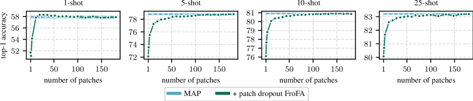
Figure 5: Average top-1 accuracy for patch dropout FroFA on our ILSVRC-2012 test set. We use the JFT-3B L/16 base setup (cf. Sec. 5). We sweep across a base sweep (cf. Sec. 4.4) to first find the best setting on our ILSVRC-2012 validation set for each number of patches (cf. Sec. S2.2). Shaded areas indicate standard errors collected via sampling each shot five times.

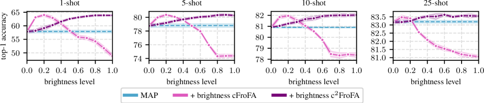
Figure 6: Average top-1 accuracy for channel variants (c/c²) of brightness FroFA on our ILSVRC-2012 test set. We use the JFT-3B L/16 base setup (cf. Sec. 5). We sweep across a base sweep (cf. Sec. 4.4) to first find the best setting on our ILSVRC-2012 validation set for each brightness level (cf. Sec. S2.2). Shaded areas indicate standard errors collected via sampling each shot five times.

S2.3 Training Details

Pretraining: In the JFT-3B setup, we use pretrained models from Zhai et al. [71]. The models are pretrained using a sigmoid cross-entropy loss. The weights are optimized by Adafactor [58], however, with slight modifications, including the use of the first momentum (in half-precision) by setting $\beta_{1}=0.9$ (instead of discarding it by $\beta_{1}=0$), disabling weight norm-based learning rate scaling, and limiting the second momentum decay to $\beta_{2}=0.999$. Further, weight decay is applied with 3.0 on the head and 0.03 for the rest of the remaining network weights. The learning rate is adapted by a reciprocal square-root schedule for 4,000,000 steps with a linear warm-up phase of 10,000 steps and a linear cool-down phase of 50,000 steps. The starting learning rate is set to 0.0008 for all model sizes (Ti/16, B/16, and L/16). The images are preprocessed by an $224\!\times\!224$ inception-style crop and a random horizontal flip. We set the batch size to 4,096. To stabilize training, a global norm clipping of 1.0 is used.

In the ImageNet-21k setup, we follow settings from Steiner et al. [60] and use a sigmoid cross-entropy loss for multi-label pretraining. We use the Adam optimizer [31] in half-precision mode and set $\beta_{1}=0.9$ and $\beta_{2}=0.999$. Further, we apply (decoupled) weight decay [45] with either 0.03 for Ti/16 or 0.1 for B/16 and L/16. We adapt the learning rate using a cosine schedule for roughly 930,000 steps (300 epochs) with a linear warm-up phase of 10,000 steps. We set the starting learning rate to 0.001 for all models. During preprocessing, we crop the images to $224\!\times\!224$ following an inception-style crop and a random horizontal flip. While we don’t use any additional augmentation for Ti/16, we follow suggestions by Steiner et al. [60] and use the ‘light1’ and ‘medium2’ augmentation settings for B/16 and L/16 ViTs, respectively. Finally, we use a batch size of 4,096 and stabilize training by using a global norm clipping of 1.0.

In the WebLI setup, we use a pretrained vision-language model from Zhai et al. [72]. The model consists of an L/16 ViT, later used in our experiments for few-shot transfer learning, and an L-sized transformer [64] for text embeddings. Similar to the JFT-3B training setup, the Adafactor optimizer is used with first momentum (in half-precision) and $\beta_{1}=0.9$, disabled weight norm-based learning rate scaling, and limitation of the second momentum decay to $\beta_{2}=0.999$. Further, weight decay is applied with 0.0001 and the learning rate is adapted by a reciprocal square-root schedule with a linear warm-up phase of 50,000 steps and a linear cool-down phase of 50,000 steps. The starting learning rate is set to 0.001. The images are resized to $256\!\times\!256$ while the text is tokenized into 64 tokens by SentencePiece [34] trained on the English C4 dataset [53] using a vocabulary size of 32,000. The training is limited to 40 billion examples and a batch size of 32,768 is used.

Few-shot transfer learning: We first process each few-shot dataset through a pretrained model and store the extracted features (cf. Fig. 2). We resize each image to $224\!\times\!224$ before feeding it to the model.

We follow up with a training where we mostly use transfer learning settings from Steiner et al. [60]. We use a sigmoid cross-entropy loss. This might be non-intuitive given that all of our few-shot datasets are not multi-labeled. However, we didn’t really observe any performance drops compared to using the more common softmax cross-entropy loss, so we stick to the sigmoid cross-entropy loss. We use stochastic gradient descent with momentum of 0.9. Similar to the pretraining setup, we also store internal optimizer states in half-precision. Except for the experiment series in Secs. 6 and 7, we do not apply any weight decay. The learning rate is adapted following a cosine schedule with a linear warm-up phase of 500 steps. In addition, we stabilize training by using a global norm clipping of 1.0. Further, we sweep across batch size, learning rate and number of steps yielding 100 combinations (cf. Sec. 4.4) for each shot.

S3 Additional Experiments and Results

In this section, we show additional experimental results.

S3.1 Patch Dropout and Brightness

In Fig. 3, we only report results for 1- and 25-shot settings using patch dropout FroFA and brightness (c/c²)FroFA. We extend this by also reporting results for 5- and 10-shot settings in Figs. 6 and 5. The observations from Fig. 3 on 1- and 25-shot also transfer to 5- and 10-shot.

			JFT-3B					ImageNet-21k
Model	Method		1-shot	5-shot	10-shot	25-shot		1-shot	5-shot	10-shot	25-shot
Ti/16	MAPwd		19.1	46.4	*53.6*	*60.2*		20.5	53.6	59.7	64.9
	Linear probe		33.0	48.0	52.2	55.4		36.8	53.7	58.0	61.1
	MAPwd + FroFA		20.3	47.2	*53.6*	*60.1*		22.1	54.9	60.1	65.2
B/16	MAPwd		*51.3*	74.8	77.5	*79.8*		*31.3*	71.7	75.3	78.1
	Linear probe		59.6	74.5	76.9	78.3		52.2	72.9	76.0	77.9
	MAPwd + FroFA		*52.4*	75.2	77.8	*79.9*		*30.6*	73.4	76.3	78.3
L/16	MAPwd		61.8	79.8	81.5	83.4		*38.8*	75.9	78.6	80.7
	Linear probe		66.5	79.6	81.5	82.4		54.7	77.1	79.8	*81.1*
	MAPwd + FroFA		63.9	80.4	82.0	83.6		*39.3*	78.0	80.0	*81.2*

Table 9: Average top-1 accuracy for JFT-3B and ImageNet-21k ViTs on our ILSVRC-2012 test set trained on few-shotted ILSVRC-2012 training sets, complementing Fig. 4. We report results for the weight-decayed MAP, i.e. MAP^wd, and L2-regularized linear probe baseline, as well as our best FroFA-based approach, i.e., weight-decayed MAP combined with brightness c²FroFA (MAP^wd + FroFA). The best results per shot are boldfaced. Each shot is sampled five times and an asterisk (*) indicates that the improvement of ‘MAP^wd + FroFA’ to ‘MAP^wd’or ‘linear probe’ is not statistically significant under a two-tailed t-test with 95% confidence.

S3.2 Advanced FroFA Protocols

In Tab. 10, we report results for our RandAugment (RA^∗) and TrivialAugment (TA^∗) variations from Sec. S2.2. We did not average across five runs and thus only report absolute gains with respect to a reference run. Therefore, numbers which are reported in the main paper, e.g., in Tab. 4, are slightly different. Overall, we observe that both RA^∗ and TA^∗ do not improve upon the best single augmentation, i.e., brightness c²FroFA (Bc²). We also observe that increasing the set of augmentations from $\mathcal{A}_{\mathrm{top}2}$ to $\mathcal{A}_{\mathrm{top}3}$ rather worsens the performance for both RA^∗ and TA^∗.

RA^∗ TA^∗ Shots MAP Bc² $\mathcal{A}_{\mathrm{top}2}$ $\mathcal{A}_{\mathrm{top}3}$ $\mathcal{A}_{\mathrm{top}2}$ $\mathcal{A}_{\mathrm{top}3}$ 1 58.4 $+$6.0 $+$3.9 $+$2.4 $+$4.8 $+$4.3 5 79.1 $+$1.5 $+$1.0 $+$0.4 $+$1.4 $+$1.2 10 80.7 $+$1.3 $+$1.0 $+$0.6 $+$1.4 $+$1.4 25 83.0 $+$0.6 $+$0.4 $+$0.0 $+$0.5 $+$0.4

Table 10: Top-1 accuracy for advanced FroFA protocols on our ILSVRC-2012 test set. Absolute gains to the MAP baseline (reference run) are reported. We use the JFT-3B L/16 base setup (cf. Sec. 5). We compare brightness c²FroFA (Bc²) with our variations of RandAugment (RA^∗) and TrivialAugment (TA^∗), cf. Sec. S2.2. For the latter, we either use the top-2 ($\mathcal{A}_{\mathrm{top}2}$) or top-3 ($\mathcal{A}_{\mathrm{top}3}$) augmentations. The best results per shot are boldfaced (multiple ones if close, i.e., $\pm$0.2).

S3.3 ILSVRC-2012 Results

In Tab. 9, we give more detailed results for Fig. 4, i.e., Ti/16, B/16, and L/16 pretrained on either ImageNet-21k or JFT-3B and subsequently finetuned on few-shotted ILSVRC-2012 training sets. Numbers for the two baselines, i.e., weight-decayed MAP (MAP^wd) and L2-regularized linear probe, and our best method, i.e., MAP^wd combined with brightness c²FroFA (MAP^wd + FroFA), are reported. As before, we observe that linear probe is particularly strong on 1-shot while our method is on par or favorable to MAP^wd and linear probe on 5- to 25-shot settings.

S3.4 Results for Seven Other Few-Shot Datasets

In Fig. 1 and Tab. 5 we report mean results across seven few-shot datasets for ‘MAP^wd’, ‘linear probe’, and ‘MAP^wd + FroFA’ using frozen features from a JFT-3B or WebLI-SigLIP L/16 ViT. In Tabs. 11 and 12 we complement these with exact numbers for each dataset and shot.

We first look at JFT-3B results (Tab. 11). Similar to Tab. 5 (upper half) and Fig. 1 (left), we observe that on average our method, i.e., ‘MAP^wd + FroFA’, significantly surpasses both MAP^wd and linear probe across all shots. A closer look at the individual datasets reveals that in some settings linear probe is the best (e.g., SUN397, 1-shot). Further, DMLab seems to show not a clear trend. However, in most settings we observe that ‘MAP^wd + FroFA’ is either better or at least maintains the performance. In general, a similar observation can be made on the WebLI-SigLIP setting (cf. Tab. 12). For example, DMLab seems to be a clear outlier since MAP^wd and ‘MAP^wd + FroFA’ more or less perform on par, except for 25-shot. Overall, we observe that ‘MAP^wd + FroFA’ is either better or at least maintains the performance.

Trans. dataset	Method	1-shot	5-shot	10-shot	25-shot
CIFAR10	MAPwd	81.6	97.0	97.1	97.5
	Linear probe	80.9	94.1	96.7	97.3
	MAPwd + FroFA	89.7	97.4	97.7	97.8
CIFAR100	MAPwd	63.4	82.9	85.4	86.7
	Linear probe	58.4	80.9	83.8	85.1
	MAPwd + FroFA	67.3	84.1	86.1	86.9
DMLab	MAPwd	24.3	28.8	*27.5*	*35.7*
	Linear probe	24.0	26.3	25.6	30.9
	MAPwd + FroFA	25.4	27.2	*27.8*	*35.6*
DTD	MAPwd	47.5	68.6	74.0	80.7
	Linear probe	46.9	65.9	71.3	77.3
	MAPwd + FroFA	53.0	70.8	75.3	81.7
Resisc45	MAPwd	61.6	*86.7*	*89.1*	*91.0*
	Linear probe	67.1	85.6	88.2	91.0
	MAPwd + FroFA	66.0	*87.0*	*89.4*	*91.1*
SUN397	MAPwd	51.3	74.0	77.5	80.6
	Linear probe	56.7	70.9	75.6	78.6
	MAPwd + FroFA	56.3	75.6	78.9	81.2
SVHN	MAPwd	*16.9*	22.9	27.2	46.2
	Linear probe	11.8	15.0	18.7	21.5
	MAPwd + FroFA	*16.4*	29.0	40.9	50.0
Mean	MAPwd	49.5	65.8	68.3	74.1
	Linear probe	49.1	62.7	65.7	68.8
	MAPwd + FroFA	53.4	67.3	70.9	74.9

Table 11: Average top-1 accuracy of our best FroFA combined with weight decay for seven transfer datasets using a JFT-3B L/16 ViT, complementing Fig. 1 (left) and Tab. 5 (upper half). Results are reported on the respective test set (cf. Tab. 6). We compare results to a weight-decayed MAP baseline, i.e., MAP^wd, and an L2-regularized linear probe. Per shot and dataset, the best result is boldfaced. We run ‘MAP^wd’ and ‘MAP^wd + FroFA’ experiments with five seeds. An asterisk (*) indicates that the improvement of ‘MAP^wd + FroFA’ to ‘MAP^wd’ is not statistically significant under a two-tailed t-test with 95% confidence.

Trans. dataset	Method	1-shot	5-shot	10-shot	25-shot
CIFAR10	MAPwd	71.7	88.7	91.4	93.6
	Linear probe	74.4	88.2	91.5	93.5
	MAPwd + FroFA	77.9	92.6	93.4	94.2
CIFAR100	MAPwd	45.1	73.2	75.3	78.7
	Linear probe	52.5	72.4	76.7	77.7
	MAPwd + FroFA	55.5	74.6	77.4	79.2
DMLab	MAPwd	*23.3*	*28.1*	*29.0*	35.4
	Linear probe	21.9	25.5	27.7	30.7
	MAPwd + FroFA	*22.6*	*25.9*	*29.6*	34.0
DTD	MAPwd	52.7	71.7	77.6	82.9
	Linear probe	50.6	70.6	76.5	81.8
	MAPwd + FroFA	59.4	76.1	80.0	84.1
Resisc45	MAPwd	*65.2*	83.7	*91.0*	92.6
	Linear probe	70.5	86.4	89.4	92.2
	MAPwd + FroFA	*65.1*	87.2	*91.1*	93.0
SUN397	MAPwd	42.0	69.5	75.7	79.4
	Linear probe	50.1	68.7	74.2	77.4
	MAPwd + FroFA	42.6	73.9	77.3	79.9
SVHN	MAPwd	21.6	58.7	62.7	62.8
	Linear probe	23.5	43.3	48.8	54.6
	MAPwd + FroFA	36.3	62.3	65.6	67.5
Mean	MAPwd	45.9	67.7	71.8	75.1
	Linear probe	49.1	65.0	69.3	72.6
	MAPwd + FroFA	51.3	70.4	73.5	76.0

Table 12: Average top-1 accuracy of our best FroFA combined with weight decay for all transfer datasets using a WebLI-SigLIP ViT, complementing Fig. 1 (right) and Tab. 5 (lower half). Results are reported on the respective test set (cf. Tab. 6). We compare results to a weight-decayed MAP baseline, i.e., MAP^wd, and an L2-regularized linear probe. Per shot and dataset, the best result is boldfaced. We run ‘MAP^wd’ and ‘MAP^wd + FroFA’ experiments with five seeds. An asterisk (*) indicates that the improvement of ‘MAP^wd + FroFA’ to ‘MAP^wd’ is not statistically significant under a two-tailed t-test with 95% confidence.

S3.5 Reducing the Hyperparameter Sweep

Across all experiments, we first tune our baseline extensively on a designated validation set to get the best possible accuracy and then report results on the respective test set. We apply the same protocol to tune FroFA for a fair comparison. However, since our hyperparameter sweeps are considerably large, it might raise concerns of overtuning the hyperparameters. To address this potential concern, we measure the sensitivity of our hyperparameter sweep by repeating the experiment series from Tab. 11 with a smaller sweep of 8 instead of 100 configurations: two batch sizes (32 and 512), two learning rates (0.01 and 0.03), and two training step settings (1,000 and 16,000). The absolute improvements over the MAP baseline averaged across the seven datasets from Tab. 11 are 3.7%, 3.7%, 3.2%, and 2.6% in the 1-, 5-, 10-, and 25-shot, respectively. Thus, our improvements remain consistent even with this much smaller hyperparameter sweep. We did not use weight decay in these experiments but expect a similar conclusion if weight decay is enabled.

S3.6 Comparison to Input Data Augmentations

In the following, we focus on a comparison between input data augmentations (IDAs) and frozen feature augmentations (FroFAs). As a prerequisite, we first compare the memory requirements of IDAs to FroFAs in a cached-feature setup.

Let $\mathcal{D}$ be a dataset with $D$ images where a cached frozen feature requires memory of size $M$. Training a model for $T$ epochs on $N$ different IDAs and $K$ different augmentation settings requires $D\times M\times T\times N\times K$ memory, since we need to store all variations of the dataset. With FroFA, however, a single copy of the dataset is sufficient, since the augmentations are directly applied on the cached frozen features during training. Thus, FroFA is $T\times N\times K$ more efficient compared to IDA in a cached-feature setup.

Next, we evaluate two IDAs, brightness (base augmentation of our best FroFA) and RandAugment [13] (a popular IDA), using a hyperparameter sweep comparable to the brightness c²FroFA sweep (without weight decay). In all our settings, we train the MAP head on the output of the last transformer block, i.e., our standard cached-feature setup (cf. Fig. 2). We did not average across five runs and thus only report absolute gains with respect to a reference run. Across all setups, we observe a reduction in accuracy from brightness c²FroFA (cf. Tab. 13). Notably, performance drops by more than 5% when applying brightness or RandAugment IDA on ILSVRC-2012, 10-shot. This aligns with prior work [23] showing poorer pretrained network performance on diverse augmented images.

In summary, we observe that FroFA strongly outperforms IDAs in a cached-feature setup.

S3.7 Additional FroFA Techniques

We extend our investigations in Tab. 2 with uniform noise and channel dropout FroFAs (details in Tab. 8) and show the absolute improvements in accuracy to our best FroFA, i.e., brightness c²FroFA, in Tab. 14. We did not average across five runs and thus only report absolute gains with respect to a reference run. While channel dropout performs comparable to brightness c²FroFA on 25-shot, in all other setups, channel dropout and uniform noise perform worse with performance drops ranging from 0.8% to 4.5% absolute.

S4 Final Remarks

We would like to thank the reviewers for suggesting to provide additional comparisons to input data augmentations, statistical significance tests, more details on the hyperparameter sweep, additional feature augmentation techniques and a discussion on a few missing related works. The main paper already shows a clear tendency of frozen feature augmentations in a cached-feature setup. The additional experiments carried out in the Supplementary further highlight this tendency which makes our case even stronger.

Dataset	IDA	1-shot	5-shot	10-shot	25-shot
Mean across 7	Brightness	$-$5.6	$-$0.7	$-$0.7	$-$0.3
SUN397	RandAugment	$-$6.2	$-$4.6	$-$3.6	$-$2.1
ILSVRC-2012	Brightness	$-$14.1	$-$9.7	$-$6.7	$-$5.2
	RandAugment	$-$14.2	$-$10.1	$-$6.9	$-$4.5

Table 13: Ablation on input data augmentations (IDAs). We report absolute gains in top-1 accuracy (in %) on our ILSVRC-2012 test set w.r.t. our best FroFA setting (Tab. 3, brightness c²FroFA) using a JFT-3B L/16 ViT. Negative numbers indicate that our proposed approach, i.e., brightness c²FroFA, is better. ‘Mean across 7’ incorporates all few-shot datasets, except ILSVRC-2012.

Dataset	FroFA	1-shot	5-shot	10-shot	25-shot
ILSVRC-2012	Uniform noise	$-$4.5	$-$2.3	$-$1.5	$-$1.0
	Channel dropout	$-$4.5	$-$1.1	$-$0.8	$-$0.0

Table 14: Ablation on additional frozen feature augmentations (FroFAs). We report absolute gains in top-1 accuracy (in %) on our ILSVRC-2012 test set w.r.t. our best FroFA setting (Tab. 3, brightness c²FroFA) using a JFT-3B L/16 ViT. Negative numbers indicate that our proposed approach, i.e., brightness c²FroFA, is better.

References

- Alex Krizhevsky [2009] Alex Krizhevsky. Learning Multiple Layers of Features From Tiny Images, 2009.
- Bateni et al. [2020] Peyman Bateni, Raghav Goyal, Vaden Masrani, Frank Wood, and Leonid Sigal. Improved Few-Shot Visual Classification. In Proc. of CVPR, pages 14481–14490, virtual, 2020.
- Beattie et al. [2016] Charles Beattie, Joel Z. Leibo, Denis Teplyashin, Tom Ward, Marcus Wainwright, Heinrich Küttler, Andrew Lefrancq, Simon Green, Víctor Valdés, Amir Sadik, Julian Schrittwieser, Keith Anderson, Sarah York, Max Cant, Adam Cain, Adrian Bolton, Stephen Gaffney, Helen King, Demis Hassabis, Shane Legg, and Stig Petersen. DeepMind Lab. arXiv, 1612.03801:1–11, 2016.
- Beyer et al. [2022] Lucas Beyer, Xiaohua Zhai, and Alexander Kolesnikov. Better Plain ViT Baselines for ImageNet-1k. arXiv, 2205.01580:1–3, 2022.
- Chen et al. [2022] Shoufa Chen, Chongjian Ge, Zhan Tong, Jiangliu Wang, Yibing Song, Jue Wang, and Ping Luo. AdaptFormer: Adapting Vision Transformers for Scalable Visual Recognition. In Proc. of NeurIPS, pages 16664–16678, New Orleans, LA, USA, 2022.
- Chen et al. [2023] Xi Chen, Xiao Wang, Soravit Changpinyo, AJ Piergiovanni, Piotr Padlewski, Daniel Salz, Sebastian Goodman, Adam Grycner, Basil Mustafa, Lucas Beyer, Alexander Kolesnikov, Joan Puigcerver, Nan Ding, Keran Rong, Hassan Akbari, Gaurav Mishra, Linting Xue, Ashish Thapliyal, James Bradbury, Weicheng Kuo, Mojtaba Seyedhosseini, Chao Jia, Burcu Karagol Ayan, Carlos Riquelme, Andreas Steiner, Anelia Angelova, Xiaohua Zhai, Neil Houlsby, and Radu Soricut. PaLI: A Jointly Scaled Multilingual Language-Image Model. In Proc. of ICLR, pages 1–33, Kigali, Rwanda, 2023.
- Cheng et al. [2017] Gong Cheng, Junwei Han, and Xiaoqiang Lu. Remote Sensing Image Scene Classification: Benchmark and State of the Art. Proc. IEEE, 105(10):1865–1883, 2017.
- Cherti et al. [2023] Mehdi Cherti, Romain Beaumont, Ross Wightman, Mitchell Wortsman, Gabriel Ilharco, Cade Gordon, Christoph Schuhmann, Ludwig Schmidt, and Jenia Jitsev. Reproducible Scaling Laws for Contrastive Language-Image Learning. In Proc. of CVPR, pages 2818–2829, Vancouver, BC, Canada, 2023.
- Cheung and Yeung [2021] Tsz-Him Cheung and Dit-Yan Yeung. MODALS: Modality-agnostic Automated Data Augmentation in the Latent Space. In Proc. of ICLR, pages 1–18, virtual, 2021.
- Chollet [2017] François Chollet. Xception: Deep Learning with Depthwise Separable Convolutions. In Proc. of CVPR, pages 1063–6919, Honolulu, HI, USA, 2017.
- Cimpoi et al. [2014] Mircea Cimpoi, Subhransu Maji, Iasonas Kokkinos, Sammy Mohamed, and Andrea Vedaldi. Describing Textures in the Wild. In Proc. of CVPR, pages 3606–3613, Columbus, OH, USA, 2014.
- Cubuk et al. [2019] Ekin D. Cubuk, Barret Zoph, Dandelion Mane, Vijay Vasudevan, and Quoc V. Le. AutoAugment: Learning Augmentation Strategies From Data. In Proc. of CVPR, pages 113–123, Long Beach, CA, USA, 2019.
- Cubuk et al. [2020] Ekin Dogus Cubuk, Barret Zoph, Jon Shlens, and Quoc Le. RandAugment: Practical Automated Data Augmentation with a Reduced Search Space. In Proc. of NeurIPS, pages 18613–18624, virtual, 2020.
- Dai et al. [2021] Zihang Dai, Hanxiao Liu, Quoc V. Le, and Mingxing Tan. CoAtNet: Marrying Convolution and Attention for All Data Sizes. In Proc. of NeurIPS, pages 3965–3977, virtual, 2021.
- Dehghani et al. [2022] Mostafa Dehghani, Alexey Gritsenko, Anurag Arnab, Matthias Minderer, and Yi Tay. Scenic: A JAX Library for Computer Vision Research and Beyond. In Proc. of CVPR, pages 21393–21398, New Orleans, LA, USA, 2022.
- Dehghani et al. [2023] Mostafa Dehghani, Josip Djolonga, Basil Mustafa, Piotr Padlewski, Jonathan Heek, Justin Gilmer, Andreas Peter Steiner, Mathilde Caron, Robert Geirhos, Ibrahim Alabdulmohsin, Rodolphe Jenatton, Lucas Beyer, Michael Tschannen, Anurag Arnab, Xiao Wang, Carlos Riquelme Ruiz, Matthias Minderer, Joan Puigcerver, Utku Evci, Manoj Kumar, Sjoerd Van Steenkiste, Gamaleldin Fathy Elsayed, Aravindh Mahendran, Fisher Yu, Avital Oliver, Fantine Huot, Jasmijn Bastings, Mark Collier, Alexey A. Gritsenko, Vighnesh Birodkar, Cristina Nader Vasconcelos, Yi Tay, Thomas Mensink, Alexander Kolesnikov, Filip Pavetic, Dustin Tran, Thomas Kipf, Mario Lucic, Xiaohua Zhai, Daniel Keysers, Jeremiah J. Harmsen, and Neil Houlsby. Scaling Vision Transformers to 22 Billion Parameters. In Proc. of ICML, pages 7480–7512, Honolulu, HI, USA, 2023.
- Deng et al. [2009] Jia Deng, Wei Dong, Richard Socher, Li-Jia Li, Kai Li, and Li Fei-Fei. ImageNet: A Large-Scale Hierarchical Image Database. In Proc. of CVPR, pages 248–255, Miami, FL, USA, 2009.
- DeVries and Taylor [2017] Terrance DeVries and Graham W. Taylor. Dataset Augmentation in Feature Space. In Proc. of ICLR - Workshops, pages 1–12, Toulon, France, 2017.
- Dosovitskiy et al. [2021] Alexey Dosovitskiy, Lucas Beyer, Alexander Kolesnikov, Dirk Weissenborn, Xiaohua Zhai, Thomas Unterthiner, Mostafa Dehghani, Matthias Minderer, Georg Heigold, Sylvain Gelly, Jakob Uszkoreit, and Neil Houlsby. An Image Is Worth 16x16 Words: Transformers for Image Recognition at Scale. In Proc. of ICLR, pages 1–21, virtual, 2021.
- Dumoulin et al. [2021] Vincent Dumoulin, Neil Houlsby, Utku Evci, Xiaohua Zhai, Ross Goroshin, Sylvain Gelly, and Hugo Larochelle. A Unified Few-Shot Classification Benchmark to Compare Transfer and Meta Learning Approaches. In Proc. of NeurIPS - Datasets and Benchmarks Track, pages 1–14, virtual, 2021.
- Gani et al. [2022] Hanan Gani, Muzammal Naseer, and Mohammad Yaqub. How to Train Vision Transformer on Small-Scale Datasets? In Proc. of BMVC, pages 1–16, London, UK, 2022.
- Gao et al. [2023] Peng Gao, Shijie Geng, Renrui Zhang, Teli Ma, Rongyao Fang, Yongfeng Zhang, Hongsheng Li, and Yu Qiao. CLIP-Adapter: Better Vision-Language Models with Feature Adapters. Int. J. Comput. Vis., 132(2):581–595, 2023.
- Gontijo-Lopes et al. [2021] Raphael Gontijo-Lopes, Sylvia Smullin, Ekin Dogus Cubuk, and Ethan Dyer. Tradeoffs in Data Augmentation: An Empirical Study. In Proc. of ICLR, pages 1–27, virtual, 2021.
- Grave et al. [2017] Edouard Grave, Armand Joulin, and Nicolas Usunier. Improving Neural Language Models with a Continuous Cache. In Proc. of ICLR, pages 1–9, Toulon, France, 2017.
- He et al. [2023] Xuehai He, Chuanyuan Li, Pengchuan Zhang, Jianwei Yang, and Xin Eric Wang. Parameter-Efficient Model Adaptation for Vision Transformers. In Proc. of AAAI, pages 817–825, Washington, DC, USA, 2023.
- Hendrycks et al. [2020] Dan Hendrycks, Norman Mu, Ekin D. Cubuk, Barret Zoph, Justin Gilmer, and Balaji Lakshminarayanan. AugMix: A Simple Data Processing Method to Improve Robustness and Uncertainty. In Proc. of ICLR, pages 1–15, Virtual, 2020.
- Hinton et al. [2014] Geoffrey Hinton, Oriol Vinyals, and Jeff Dean. Distilling Knowledge in a Neural Network. In Proc. of NIPS - Workshops, pages 1–9, Montréal, QC, Canada, 2014. (In 2018, ‘NIPS’ was renamed to ‘NeurIPS’).
- Houlsby et al. [2019] Neil Houlsby, Andrei Giurgiu, Stanislaw Jastrzebski, Bruna Morrone, Quentin de Laroussilhe, Andrea Gesmundo, Mona Attariyan, and Sylvain Gelly. Parameter-Efficient Transfer Learning for NLP. In Proc. of ICML, pages 2790–2799, Long Beach, CA, USA, 2019.
- Hu et al. [2022] Edward J. Hu, Yelong Shen, Phillip Wallis, Zeyuan Allen-Zhu, Yuanzhi Li, Shean Wang, Lu Wang, and Weizhu Chen. LoRA: Low-Rank Adaptation of Large Language Models. In Proc. of ICLR, pages 1–13, virtual, 2022.
- Jia et al. [2022] Menglin Jia, Luming Tang, Bor-Chun Chen, Claire Cardie, Serge Belongie, Bharath Hariharan, and Ser-Nam Lim. Visual Prompt Tuning. In Proc. of ECCV, pages 709–727, Tel Aviv, Israel, 2022.
- Kingma and Ba [2015] Diederik P. Kingma and Jimmy Ba. Adam: A Method for Stochastic Optimization. In Proc. of ICLR, pages 1–15, San Diego, CA, USA, 2015.
- Kolesnikov et al. [2020] Alexander Kolesnikov, Lucas Beyer, Xiaohua Zhai, Joan Puigcerver, Jessica Yung, Sylvain Gelly, and Neil Houlsby. Big Transfer (BiT): General Visual Representation Learning. In Proc. of ECCV, pages 491–507, virtual, 2020.
- Kossen et al. [2023] Jannik Kossen, Mark Collier, Basil Mustafa, Xiao Wang, Xiaohua Zhai, Lucas Beyer, Andreas Steiner, Jesse Berent, Rodolphe Jenatton, and Efi Kokiopoulou. Three Towers: Flexible Contrastive Learning with Pretrained Image Models. In Proc. of NeurIPS, pages 31340–31371, New Orleans, LA, USA, 2023.
- Kudo and Richardson [2018] Taku Kudo and John Richardson. SentencePiece: A Simple and Language-Independent Subword Tokenizer and Detokenizer for Neural Text Processing. In Proc. of EMNLP - System Demonstrations, pages 66–71, Brussels, Belgium, 2018.
- Kumar et al. [2019] Varun Kumar, Hadrien Glaude, Cyprien de Lichy, and Wlliam Campbell. A Closer Look At Feature Space Data Augmentation For Few-Shot Intent Classification. In Proc. of EMNLP - Workshops, pages 1–10, Hong Kong, China, 2019.
- Lake et al. [2019] Brenden M. Lake, Ruslan Salakhutdinov, and Joshua B. Tenenbaum. The Omniglot Challenge: A 3-year Progress Report. Curr. Opin. Behav. Sci., 29:97–104, 2019.
- Lee et al. [2019] Juho Lee, Yoonho Lee, Jungtaek Kim, Adam Kosiorek, Seungjin Choi, and Yee Whye Teh. Set Transformer: A Framework for Attention-Based Permutation-Invariant Neural Networks. In Proc. of ICML, pages 3744–3753, Long Beach, CA, USA, 2019.
- Lee et al. [2021] Seung Hoon Lee, Seunghyun Lee, and Byung Cheol Song. Vision Transformer for Small-Size Datasets. arXiv, 2112.13492:1–11, 2021.
- Lester et al. [2021] Brian Lester, Rami Al-Rfou, and Noah Constant. The Power of Scale for Parameter-Efficient Prompt Tuning. In Proc. of EMNLP, pages 3045–3059, virtual, 2021.
- Liu et al. [2018] Xiaofeng Liu, Yang Zou, Lingsheng Kong, Zhihui Diao, Junliang Yan, Jun Wang, Site Li, Ping Jia, and Jane You. Data Augmentation via Latent Space Interpolation for Image Classification. In Proc. of ICPR, pages 728–733, Beijing, China, 2018.
- Liu et al. [2021a] Yahui Liu, Enver Sangineto, Wei Bi, Nicu Sebe, Bruno Lepri, and Marco De Nadai. Efficient Training of Visual Transformers with Small Datasets. In Proc. of NeurIPS, pages 23818–23830, virtual, 2021a.
- Liu et al. [2023a] Yue Liu, Christos Matsoukas, Fredrik Strand, Hossein Azizpour, and Kevin Smith. PatchDropout: Economizing Vision Transformers Using Patch Dropout. In Proc. of WACV, pages 3942–3951, Waikoloa, HI, USA, 2023a.
- Liu et al. [2021b] Ze Liu, Yutong Lin, Yue Cao, Han Hu, Yixuan Wei, Zheng Zhang, Stephen Lin, and Baining Guo. Swin Transformer: Hierarchical Vision Transformer Using Shifted Windows. In Proc. of ICCV, pages 10012–10022, virtual, 2021b.
- Liu et al. [2023b] Zichang Liu, Zhiqiang Tang, Xingjian Shi, Aston Zhang, Mu Li, Anshumali Shrivastava, and Andrew Gordon Wilson. Learning Multimodal Data Augmentation in Feature Space. In Proc. of ICLR, pages 1–15, Kigali, Rwanda, 2023b.
- Loshchilov and Hutter [2019] Ilya Loshchilov and Frank Hutter. Decoupled Weight Decay Regularization. In Proc. of ICLR, pages 1–18, New Orleans, LA, USA, 2019.
- Müller and Hutter [2021] Samuel G. Müller and Frank Hutter. TrivialAugment: Tuning-Free Yet State-of-the-Art Data Augmentation. In Proc. of ICCV, pages 774–782, virtual, 2021.
- Netzer et al. [2011] Yuval Netzer, Tao Wang, Adam Coates, Alessandro Bissacco, Bo Wu, and Andrew Y. Ng. Reading Digits in Natural Images with Unsupervised Feature Learning. In Proc. of NIPS - Workshops, pages 1–9, Granada, Spain, 2011. (In 2018, ‘NIPS’ was renamed to ‘NeurIPS’).
- Nichol et al. [2018] Alex Nichol, Joshua Achiam, and John Schulman. On First-Order Meta-Learning Algorithms. arXiv, 1803.02999:1–15, 2018.
- Oquab et al. [2024] Maxime Oquab, Timothée Darcet, Théo Moutakanni, Huy Vo, Marc Szafraniec, Vasil Khalidov, Pierre Fernandez, Daniel Haziza, Francisco Massa, Alaaeldin El-Nouby, Mahmoud Assran, Nicolas Ballas, Wojciech Galuba, Russell Howes, Po-Yao Huang, Shang-Wen Li, Ishan Misra, Michael Rabbat, Vasu Sharma, Gabriel Synnaeve, Hu Xu, Hervé Jegou, Julien Mairal, Patrick Labatut, Armand Joulin, and Piotr Bojanowski. DINOv2: Learning Robust Visual Features Without Supervision. Trans. Mach. Learn. Res., 1:1–32, 2024.
- Oreshkin et al. [2018] Boris N. Oreshkin, Pau Rodríguez López, and Alexandre Lacoste. TADAM: Task-Dependent Adaptive Metric for Improved Few-Shot Learning. In Proc. of NeurIPS, pages 719–729, Montréal, QC, Canada, 2018.
- Orhan [2018] Emin Orhan. A Simple Cache Model for Image Recognition. In Proc. of NeurIPS, pages 10128–10137, Montréal, Canada, 2018.
- Radford et al. [2021] Alec Radford, Jong Wook Kim, Chris Hallacy, Aditya Ramesh, Gabriel Goh, Sandhini Agarwal, Girish Sastry, Amanda Askell, Pamela Mishkin, Jack Clark, Gretchen Krueger, and Ilya Sutskever. Learning Transferable Visual Models From Natural Language Supervision. In Proc. of ICML, pages 8748–8763, virtual, 2021.
- Raffel et al. [2020] Colin Raffel, Noam Shazeer, Adam Roberts, Katherine Lee, Sharan Narang, Michael Matena, Yanqi Zhou, Wei Li, and Peter J. Liu. Exploring the Limits of Transfer Learning With a Unified Text-to-Text Transformer. J. Mach. Learn. Res., 21(140):1–67, 2020.
- Requeima et al. [2019] James Requeima, Jonathan Gordon, John Bronskill, Sebastian Nowozin, and Richard E. Turner. Fast and Flexible Multi-Task Classification Using Conditional Neural Adaptive Processes. In Proc. of NeurIPS, pages 7957–7968, Vancouver, BC, Canada, 2019.
- Ridnik et al. [2021] Tal Ridnik, Emanuel Ben-Baruch, Asaf Noy, and Lihi Zelnik-Manor. ImageNet-21K Pretraining for the Masses. In Proc. of NeurIPS - Datasets and Benchmarks Track, pages 1–12, virtual, 2021.
- Rodríguez et al. [2020] Pau Rodríguez, Issam H. Laradji, Alexandre Drouin, and Alexandre Lacoste. Embedding Propagation: Smoother Manifold for Few-Shot Classification. In Proc. of ECCV, pages 121–138, virtual, 2020.
- Russakovsky et al. [2015] Olga Russakovsky, Jia Deng, Hao Su, Jonathan Krause, Sanjeev Satheesh, Sean Ma, Zhiheng Huang, Andrej Karpathy, Aditya Khosla, Michael Bernstein, Alexander C. Berg, and Li Fei-Fei. ImageNet Large Scale Visual Recognition Challenge. Int. J. Comput. Vis., 115(3):211–252, 2015.
- Shazeer and Stern [2018] Noam Shazeer and Mitchell Stern. Adafactor: Adaptive Learning Rates with Sublinear Memory Cost. In Proc. of ICML, pages 4596–4604, Stockholm, Sweden, 2018.
- Snell et al. [2017] Jake Snell, Kevin Swersky, and Richard S. Zemel. Prototypical Networks for Few-Shot Learning. In Proc. of NIPS, pages 4077–4087, Long Beach, CA, USA, 2017. (In 2018, ‘NIPS’ was renamed to ‘NeurIPS’).
- Steiner et al. [2022] Andreas Steiner, Alexander Kolesnikov, Xiaohua Zhai, Ross Wightman, Jakob Uszkoreit, and Lucas Beyer. How to Train Your ViT? Data, Augmentation, and Regularization in Vision Transformers. Trans. Mach. Learn. Res., 5:1–16, 2022.
- Sun et al. [2017] Chen Sun, Abhinav Shrivastava, Saurabh Singh, and Abhinav Gupta. Revisiting Unreasonable Effectiveness of Data in Deep Learning Era. In Proc. of ICCV, pages 843–852, Venice, Italy, 2017.
- Szegedy et al. [2016] Christian Szegedy, Vincent Vanhoucke, Sergey Ioffe, Jon Shlens, and Zbigniew Wojna. Rethinking the Inception Architecture for Computer Vision. In Proc. of CVPR, pages 2818–2826, Las Vegas, NV, USA, 2016.
- Touvron et al. [2021] Hugo Touvron, Matthieu Cord, Matthijs Douze, Francisco Massa, Alexandre Sablayrolles, and Herve Jegou. Training Data-Efficient Image Transformers & Distillation Through Attention. In Proc. of ICML, pages 10347–10357, virtual, 2021.
- Vaswani et al. [2017] Ashish Vaswani, Noam Shazeer, Niki Parmar, Jakob Uszkoreit, Llion Jones, Aidan N. Gomez, Łukasz Kaiser, and Illia Polosukhin. Attention Is All You Need. In Proc. of NIPS, pages 5998–6008, Long Beach, CA, USA, 2017. (In 2018, ‘NIPS’ was renamed to ‘NeurIPS’).
- Verma et al. [2019] Vikas Verma, Alex Lamb, Christopher Beckham, Amir Najafi, Ioannis Mitliagkas, David Lopez-Paz, and Yoshua Bengio. Manifold Mixup: Better Representations by Interpolating Hidden States. In Proc. of ICML, pages 6438–6447, Long Beach, CA, USA, 2019.
- Vinyals et al. [2016] Oriol Vinyals, Charles Blundell, Timothy Lillicrap, koray kavukcuoglu, and Daan Wierstra. Matching Networks for One-Shot Learning. In Proc. of NIPS, pages 3637–3645, Barcelona, Spain, 2016. (In 2018, ‘NIPS’ was renamed to ‘NeurIPS’).
- Wang et al. [2021] Wenhai Wang, Enze Xie, Xiang Li, Deng-Ping Fan, Kaitao Song, Ding Liang, Tong Lu, Ping Luo, and Ling Shao. Pyramid Vision Transformer: A Versatile Backbone for Dense Prediction Without Convolutions. In Proc. of ICCV, pages 548–558, virtual, 2021.
- Xiao et al. [2010] Jianxiong Xiao, James Hays, Krista A. Ehinger, Aude Oliva, and Antonio Torralba. SUN Database: Large-Scale Scene Recognition From Abbey to Zoo. In Proc. of CVPR, pages 3485–3492, San Francisco, CA, USA, 2010.
- Xiao et al. [2016] Jianxiong Xiao, Krista A. Ehinger, James Hays, Antonio Torralba, and Aude Oliva. SUN Database: Exploring a Large Collection of Scene Categories. Int. J. Comput. Vis., 119(1):3–22, 2016.
- Zhai et al. [2020] Xiaohua Zhai, Joan Puigcerver, Alexander Kolesnikov, Pierre Ruyssen, Carlos Riquelme, Mario Lucic, Josip Djolonga, André Susano Pinto, Maxim Neumann, Alexey Dosovitskiy, Lucas Beyer, Olivier Bachem, Michael Tschannen, Marcin Michalski, Olivier Bousquet, Sylvain Gelly, and Neil Houlsby. A Large-Scale Study of Representation Learning with the Visual Task Adaptation Benchmark. arXiv, 1910.04867:1–33, 2020.
- Zhai et al. [2022] Xiaohua Zhai, Alexander Kolesnikov, Neil Houlsby, and Lucas Beyer. Scaling Vision Transformers. In Proc. of CVPR, pages 12104–12113, New Orleans, LA, USA, 2022.
- Zhai et al. [2023] Xiaohua Zhai, Basil Mustafa, Alexander Kolesnikov, and Lucas Beyer. Sigmoid Loss for Language-Image Pretraining. In Proc. of ICCV, pages 11975–11986, Paris, France, 2023.
- Zhang et al. [2018] Hongyi Zhang, Moustapha Cissé, Yann N. Dauphin, and David Lopez-Paz. Mixup: Beyond Empirical Risk Minimization. In Proc. of ICLR, pages 1–13, Vancouver, BC, Canada, 2018.
- Zhang et al. [2022] Renrui Zhang, Wei Zhang, Rongyao Fang, Peng Gao, Kunchang Li, Jifeng Dai, Yu Qiao, and Hongsheng Li. Tip-Adapter: Training-Free Adaption of CLIP for Few-Shot Classification. In Proc. of ECCV, pages 493–510, Tel Aviv, Israel, 2022.