Multilevel functional distributional models with application to continuous glucose monitoring in diabetes clinical trials

Abstract

Continuous glucose monitoring (CGM) is a minimally invasive technology that allows continuous monitoring of an individual’s blood glucose. We focus on a large clinical trial that collected CGM data every few minutes for 26 weeks and assumes that the basic observation unit is the distribution of CGM observations in a four-week interval. The resulting data structure is multilevel (because each individual has multiple months of data) and distributional (because the data for each four-week interval is represented as a distribution). The scientific goals are to: (1) identify and quantify the effects of factors that affect glycemic control in type 1 diabetes (T1D) patients; and (2) identify and characterize the patients who respond to treatment. To address these goals, we propose a new multilevel functional model that treats the CGM distributions as a response. Methods are motivated by and applied to data collected by The Juvenile Diabetes Research Foundation Continuous Glucose Monitoring Group. Reproducible code for the methods introduced here is available on GitHub.

1 Introduction

The continuous improvement and availability of wearable and implantable technology (WIT) provides new scientific and methodological opportunities Liao et al. (2019). For example, continuous glucose monitors (CGM) Burge et al. (2008) measure interstitial glucose continuously every 5 minutes, which can be used for diabetes management. The use of CGM can: (1) help inform the effect and guide the use of individualized treatments Tamborlane et al. (2008); (2) be paired with integrated systems of insulin pumps to create artificial pancreas systems Rodbard (2017); and (3) guide decisions about personalized nutrition due to the individual patient’s glycemic responses to specific food groups Leshem et al. (2020); Ben-Yacov et al. (2021).

CGM data is relatively dense (one observation every five minutes) and exhibits substantial heterogeneity and nonstationarity. This happens because nutrition, physical activity, and sleep can have a profound effect on the glucose trajectory of the individual. Moreover, the CGM trajectories are highly variable within- and between-individuals with diabetes Gaynanova et al. (2020). To avoid the problems induced by uncontrollable environmental and behavioral factors, we have replaced the raw CGM time series in free-living conditions with the density of these observations over a period of time. We labeled these distributional representations as glucodensities Matabuena et al. (2021a), which provide information about the proportion of time a patient is within each range of glucose concentrations. Here we will work with the quantile function of glucodensities, which are increasing functions of the corresponding probabilities. Distributional representation of functional data has been proposed recently in the context of objective measurements of physical activity using accelerometers Matabuena & Petersen (2023); Ghosal, Varma, Volfson, Hillel, Urbanek, Hausdorff, Watts & Zipunnikov (2021); Ghosal, Varma, Volfson, Urbanek, Hausdorff, Watts & Zipunnikov (2021); Ghosal & Matabuena (2023); Ghosal, Matabuena, Meiring & Petersen (2023); Matabuena, Félix, Hammouri, Mota & del Pozo Cruz (2022); Koffman et al. (2023), in fMRI studies Tang et al. (2020), and CGM studies. Here we will extend these ideas to the case when distributional data are observed at multiple visits within the same study participant.

Distributional representations of time series data are typically obtained over a period of time when disease evolution is unlikely and the observed variability can be assigned to natural and reversible biological changes. For example, in studies of diabetes using CGM monitoring, one could reasonably assume that the disease does not progress too much during one month, but detectable differences can be observed over longer periods of monitoring. This partition leads to a longitudinal study where the measurement at every time point (in this case a four week interval) is a distribution (the CGM distribution over a four-week period). This is a new data structure and methodological problem that occur directly from an important scientific problem. In particular, there is substantial interest in identifying the factors that affect the longitudinal dynamics of glucose and quantifying their deterministic and irreversible effects on glucose control.

To address this challenge, we propose the first multilevel functional model where the response is a quantile function, and the predictors are scalar variables. Methods are motivated by and applied to a clinical trial conducted by The Juvenile Diabetes Research Foundation Continuous Glucose Monitoring Study Group. The study evaluated the efficacy of CGM in controlling glucose in study participants with type 1 diabetes compared to a group of study participants with type 1 diabetes who were blinded to CGM information. The scientific problem is to investigate how baseline patient characteristics and CGM monitoring impact glycemic control. The study duration was 26 weeks, which for this analysis was partitioned into six four-week intervals and a single two-week period ($26=6\times 4+2$). The quantile function was calculated for every study participant and every interval to reduce the within- and between-day variability of the quantile function estimation.

2 CGM data description

Continuous Glucose Monitoring (CGM) is thought to be an important component of the future of diabetes management Burge et al. (2008); Nørgaard et al. (2023). Several studies Tamborlane et al. (2008); Wood et al. (2018); Schnell et al. (2017); Rodbard (2017); Ajjan (2017); Rodbard (2016); Bailey et al. (2015); Beck et al. (2012, 2018); Ajjan et al. (2019); Schnell et al. (2017); Burge et al. (2008) have provided evidence that the use of CGM in randomized clinical trials is feasible and can help improve glycemic control. CGM data are often analyzed using summaries Battelino et al. (2022) (such as the daily or weekly mean), which can result in substantial loss of information and may lead to clinical decisions that do not account for the complexity of the data. Indeed, it is possible to have two individuals with similar mean CGM, but with very different profiles Yoo & Kim (2020); Martens et al. (2021): one stable around the mean and another with long excursions into the hyper- and hypo-glycemic ranges. These two individuals would require different interventions, but would be indistinguishable if data were summarized as the mean CGM. Therefore, here we focus on the quantile function over a period of time (e.g., four weeks) which includes information about the mean, standard deviation (variability), and time spent in all CGM ranges.

Our research was motivated by data collected by The Juvenile Diabetes Research Foundation (JDRF) Continuous Glucose Monitoring Study Group Tamborlane et al. (2008); Juvenile Diabetes Research Foundation Continuous Glucose Monitoring Study Group (2009), one of the first studies to evaluate the potential of continuous glucose monitoring in the management of type $1$ Diabetes Mellitus (T1DM). Data were obtained from the multi-center clinical trial. A total of $451$ adults and children were randomized into two groups. The first group (treatment) received instructions for using and managing their glucose values using CGM data. The second group (control) used standard of care, which included home monitoring, but no information from CGM. In this paper we consider a subset of $349$ study participants who had enough longitudinal CGM information to construct at least six functional quantile profiles. The study enrolled study participants with baseline glycated hemoglobin (HbA1c) between $5.7$ and $10$%. HbA1c is the primary biomarker for the diagnosis and control of diabetes. According to the US Center for Disease Control “a normal A1C level is below 5.7%, a level of 5.7% to 6.4% indicates prediabetes, and a level of 6.5% or more indicates diabetes”.

The number of scheduled contacts with study staff was identical for all study participants. Visits were conducted at $1$, $4$, $8$, $13$, $19$, and $26$ weeks ($\pm 1$ week), with one telephone contact between each visit, to review glucose data and adjust diabetes management. The primary outcome of the clinical trial was the change in the mean HbA1c from baseline to twenty-six weeks, as determined by a central laboratory.

The first two publications based on these data focused on separate analyses for study participants with (HbA1c) greater than $7$% ($n_{2}=322$ study participants) and less than $7$% ($n_{1}=129$ study participants), respectively. Based on the subset of $322$ study participants with HbA1c greater than $7$% the authors reported that: (1) the changes in HbA1c varied substantially by age group (p-value=$0.003$); (2) there was a statistically significant difference in HbA1c change between groups (continuous monitoring group versus control) for individuals who were 25 years or older (mean difference in change, -$0.53$%; $95$% confidence interval [CI], -$0.71$ to -$0.35$; p-value$<0.001$); (3) there was not a statistically significant difference between groups for individuals younger than $24$. For the secondary outcome glycosylated hemoglobin a statistically significant difference was found between the groups that used and did not use information from continuous monitoring among individuals who were older than $25$. The difference was not statistically significant for individuals younger than $25$. In a subsequent paper, Juvenile Diabetes Research Foundation Continuous Glucose Monitoring Study Group (2009) focused on study participants with baseline HbA1c less than $7$% and reported a benefit for using CGM information for controlling hypoglycemia. However, hypoglycemic control depends on insulin therapy (in this case, pump systems or injections). As a larger proportion of patients use pump-systems in the treatment compared to the control group ($93$% versus $79$%), additional analyses may be necessary to understand whether differences are due to treatment (information about CGM) or to higher use of insulin pumps in the treatment group.

In this paper we analyze all patients and investigate the distribution of CGM instead of HbA1c as outcome of the study. More precisely, we partition the $26$ weeks of follow up into six four-week and one two-week intervals. In each interval we obtain the quantile function of the CGM data in that particular interval, which provides information about the time spent in any glucose range. The quantile of the time series in every interval is treated as a function. We propose to use longitudinal function-on-scalar (FoSR) regression Cui et al. (2021); Reiss et al. (2010); Shou et al. (2015); Zipunnikov et al. (2014) to study the association between CGM profiles and scalar covariates including treatment, age, sex, baseline HbA1c and insulin therapy. The model is functional because we use the entire quantile function as the outcome of interest and longitudinal because quantile functions are observed over seven periods spanning a total of $26$ weeks.

To better understand the structure of the data, Figure 1 displays the quantile functions for two patients in the treatment (top panels) and two patients in the control (bottom panels) group, respectively. Each one of these participants had only six quantile curves (CGM data for the first $24$ weeks), though other study participants had seven quantile curves ($26$ weeks). A higher quantile function corresponds to higher blood glucose for longer periods of time. This typically reflects poorer glycemic control, though in hypoglycemia ranges (blood glucose below $70$mg/dL) it reflects better glycemic control. Each quantile function is color coded to provide a temporal representation of the information. The first periods are shown in darker shades of red followed by lighter shades of red, lighter shades of blue, and darker shades of blue, respectively. For example, in the top right panel the quantile functions are higher during the first two periods (week 1-4 and week 5-8) and lower in the two subsequent periods (week 9-12 and week 13-16). The last two periods are different from each other with the fifth period (week 17-20) being higher, though not quite at the level in the first two periods. The sixth period (week 21-24) is much lower than all other periods. Overall, Figure 1 illustrates that the evolution of CGM quantiles is highly individualized and exhibits substantial heterogeneity within and between individuals.

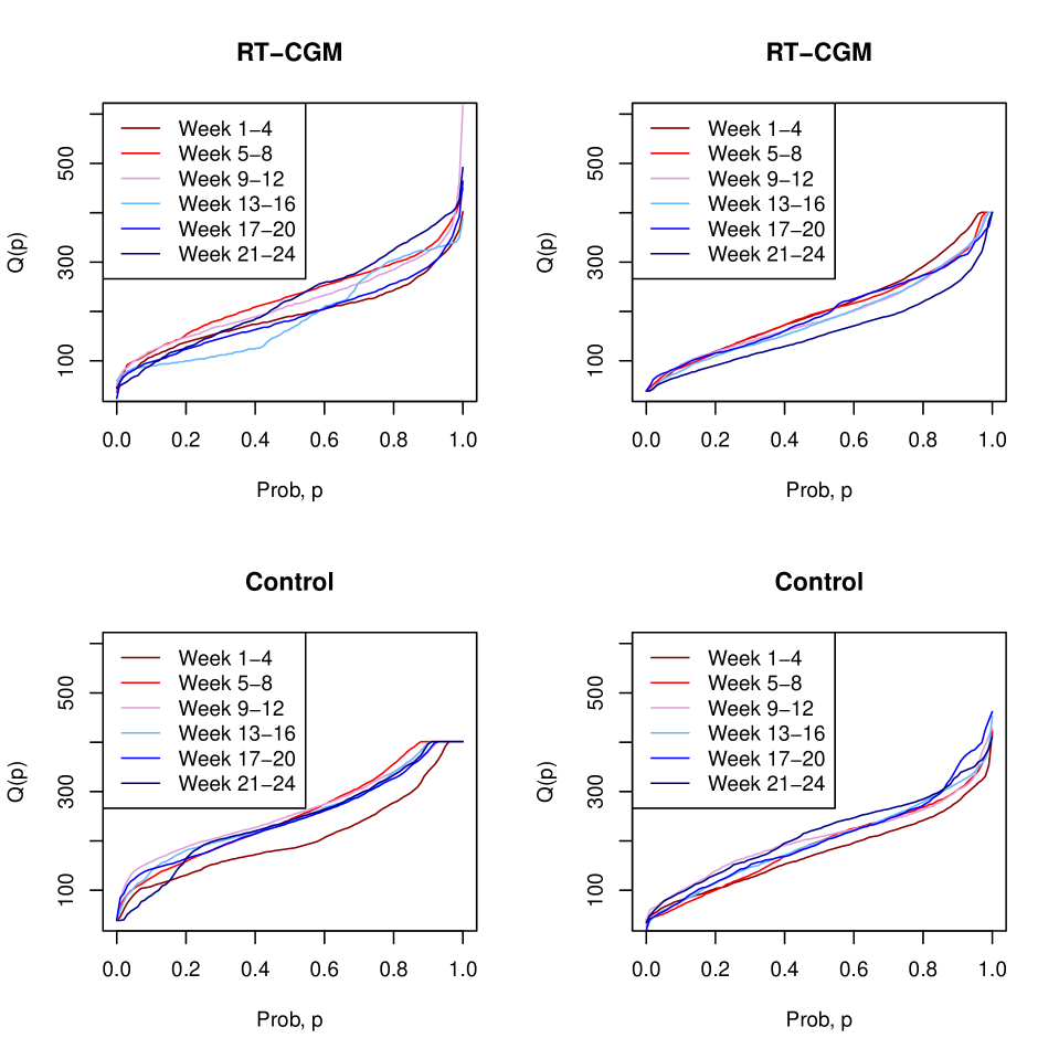
Figure 1: Example of data for four study participants of the Juvenile Diabetes Research Foundation Continuous Glucose Monitoring Study Group database in their longitudinal evolution of distributional glucose profiles during the first $24$ weeks. Top panels: two patients from the treatment group. Bottom panels: two patients from the control group.

As longitudinal functional data is quite difficult to visualize over so many study participants, we display data for a few selected CGM quantiles. More precisely, we focus on the difference between the quantiles corresponding to probabilities $0.05$, $0.50$, and $0.95$ at the end and beginning of the trial. The left panels in Figure 2 display the scatter plots of quantiles at baseline (x-axis) and end of the trial (y-axis) corresponding to the probabilities $0.05$ (top), $0.50$ (middle), and $0.95$ (bottom). Dots are color coded for the treatment group (blue) and control group (red). The left panels provide boxplots of the differences in the corresponding quantiles in the treatment and control groups, respectively. Intuitively, the goal of this paper is to provide a class of models to analyze all these quantiles simultaneously, while accounting for specific covariates.

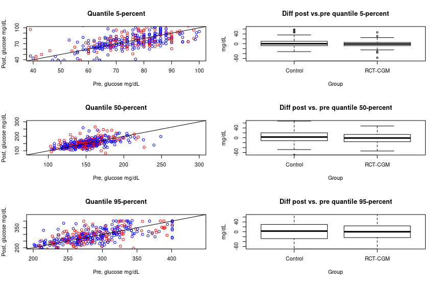
Figure 2: Population description of the CGM data analyzed in terms of the quantile of CGM time series at 5, 50, and 95 percent levels (left) in the first and last visit. Treatment group (Blue) and Control group (Red). We also show the differences between pre and post-for-the-mentioned quantile values and groups in a boxplot (right).

3 Models for longitudinal distributional representations

In this paper we will use the distribution function of CGM data, termed glucodensity (Matabuena et al., 2021b; Matabuena, Felix, Garcia-Meixide & Gude, 2022; Matabuena et al., 2023; Cui et al., 2023). Figure 3 provides an example of how the CGM time series (left panel) for a normoglycemic study participant is transformed into a density function (right panel). Formally, the space of glucodensities is defined as $\mathcal{D}=\{f\in L^{2}\left(\left[40,600\right]\right):\int_{40}^{600}f\left(s\right)ds=1\hskip 5.69046pt\text{and}\hskip 5.69046pt\int_{40}^{600}f^{2}\left(s\right)ds<\infty\}$. The values $40$ and $600$mg/dL are chosen to cover all possible glucose values, though they could be changed in particular applications.

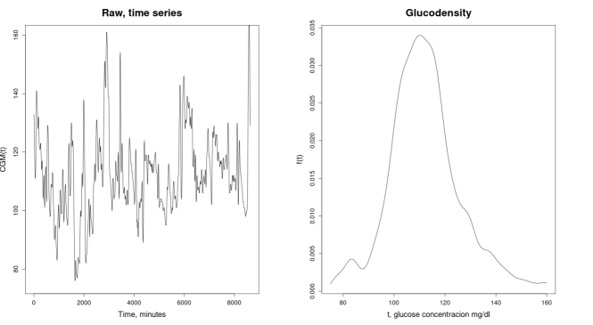
Figure 3: Left: The CGM recording from a normoglycemic patient. Right: The corresponding glucodensity.

3.1 Longitudinal Functional Quantile Models

The clinical trial study was partitioned in six four-week periods and one two-week period for a total of seven periods. In every period CGM data are sampled once every five minutes and then transformed into a quantile function. Therefore, for each study participant we have up to seven quantile functions (as some study participants do not have data in the last two-week period) that are indexed by time. This results in a longitudinal (because periods are indexed by time) quantile functional (because the measurement is the quantile function over a period) data structure. We are interested in studying the association between study participants’ covariates and the CGM quantiles observed longitudinally, while accounting for baseline, longitudinal and white noise variability Gertheiss et al. (2013).

The structure of the problem is akin to the one introduced by Greven et al. (2010). However, their primary focus was on the longitudinal decomposition of functional variability without imposing restrictions on the functional data or addressing inference for covariate effects. In the context of functional multilevel data analysis using CGM data, the methods and scientific problems are similar to the ones presented recently by Sergazinov et al. (2023). Here, we emphasize the analysis of response quantile distributional responses, as patients are monitored under real-life quantifiable scenarios typical of real-world clinical situations, rather than unconstrained functional trajectories. Furthermore, our approach allows capturing long-term changes in patients over a span of $26$ weeks, as opposed to the daily monitoring emphasized in Sergazinov et al. (2023).

More specifically, our functional data consist of quantile functions, which are inherently increasing functions. Our main focus is on identifying and quantifying the effects of covariates on CGM quantiles. The problem is also related to the one described by (Goldsmith et al., 2012; Staicu et al., 2010), though their emphasis was on longitudinal scalar-on-function rather than function-on-scalar regression. To the best of our knowledge, this is the first use of this methods in the context of CGM data for clinical diabetes trials using distributional representations of long-term CGM time series.

To introduce models for such data, we first introduce some notation. Denote by $Q_{ij}(p)$, $p\in[0,1]$, the random quantile function for individual $i=1,\ldots,n$ during period $j=1,\ldots,J_{i}$. For notation simplicity we assume that $J_{i}=J$ for all $i=1,\cdots,n$, though methods can account for a different number of observations per study participant. Consider the following multilevel functional model for $Q_{ij}(\cdot)$ Di et al. (2009)

$${}Q_{ij}(p)=\mu(p)+\nu_{j}(p)+U_{i}(p)+W_{ij}(p)\;.$$ (1)

In this model $\mu(p)$ is the global mean, $\mu(p)+\nu_{j}(p)$ is the mean during time period $j$, $U_{i}(p)$ is the subject-specific deviation from the measure-specific mean function, and $W_{ij}(p)$ is the residual subject- and period-specific deviation from the subject-specific mean. Here $\mu(p)$ and $\nu_{j}(p)$ are treated as fixed functions, while $U_{i}\left(t\right)$ and $W_{ij}(p)$ are mutually uncorrelated zero mean random functions.

In the original publication Di et al. (2009) the focus was on estimating the structure of the random processes $Z_{i}(p)$ and $W_{ij}(p)$, which was done using the eigen-decomposition of within and between-subjects variability. A much faster implementation of this model was recently proposed by Cui et al. (2022) and is accompanied by the function mfpca.face in the refund package Goldsmith et al. (2020). Here we are interested in the association between the quantile functions $Q_{ij}(p)$ and scalar covariates, while accounting for the complex longitudinal functional structure. In the next section we describe these models.

3.2 Longitudinal function-on-scalar regression models

In our case study, in addition to the quantile functional profile $Q_{ij}(p)$, we observe time dependent and independent covariates such as demographics and HbA1c. These covariates can be incorporated both in the fixed and/or random effects structure of the model. To account for these covariates we consider models of the type

$$Q_{ij}(p)=\sum_{l=1}^{L}X_{ijl}\beta_{l}(p)+\sum_{k=1}^{K}Z_{ijk}U_{ik}(p)+W_{ij}(p)\;,$$ (2)

where $X_{ijl}$ are $L$ fixed effects covariates, $\beta_{l}(p)$ is the fixed effect parameter for the quantile corresponding to probability $p$, $Z_{ijk}$ are $K$ random effects covariates, $U_{ik}(p)$ is a random functional effect corresponding to subject $i$ at probability $p$, and $W_{ij}(p)$ is the residual variation that is unexplained by either the fixed or random effects. We assume that the $U_{ik}(\cdot)$ and $W_{ij}(\cdot)$ processes are zero mean square integrable processes, with $W_{ij}(\cdot)$ being uncorrelated with all $U_{ik}(p)$, though $U_{ik}(p)$ can be correlated among themselves. We do not impose any additional restrictions on these processes, though the outcomes $Q_{ij}(p)$ are increasing functions of $p$. We propose to fit the models by ignoring this fact, produce predictions of $Q_{ij}(p)$, and then project these predictions onto the space of increasing functions.

Models such as (2) have been proposed in the literature before, are easy to write down, but are difficult to fit in real life applications. To address this problem, we adapt the recently proposed fast univariate inference (FUI) for longitudinal functional data analysis proposed by Cui et al. (2021). This approach can be implemented by fitting many pointwise mixed effects models and then smoothing the fixed effects parameters over the functional domain. An important advantage of our approach lies in its ability to generalize the intuitive method of fitting mixed effects models for each quantile separately. For practical modeling purposes using existing software, we assume that $U_{ik}(\cdot)$ and $W_{ij}(\cdot)$ are Gaussian processes. Consequently, we leverage the capabilities of specific software designed for Gaussian univariate outcomes, such as the lme4 R package.

The following algorithm was used to fit model (2):

1. For each point $p\in T_{m}=\{p_{1},\dots,p_{m}\}$, fit a separate point-wise linear mixed model using standard multilevel software for Gaussian responses, that is

   $$Q_{ij}(p)=\sum_{l=1}^{L}X_{ijl}\beta_{l}(p)+\sum_{k=1}^{K}Z_{ijk}U_{ik}(p)+W_{ij}(p).$$

2. Smooth the estimated fixed-effects coefficients $\widetilde{\beta}_{l}(p)$ using a linear smoother $\widehat{\beta}_{l}(p)=S_{l}\widetilde{\beta}_{l}$, where $S_{l}$ is a smoother that may or may not depend on $l$.

3. Use a bootstrap of study participants to conduct model inference:

   1. Bootstrap the study participants $B$ times with replacement. Calculate $\widehat{\beta}_{l}^{b}(p)$, the estimator of $\beta_{l}(p)$ conditional on the $b=1,\ldots,B$ bootstrap sample.

   2. Arrange the $\widehat{\beta}_{l}^{b}(p)$ estimators in a $B\times m$ (bootstrap samples by probabilities) and obtain the column mean $\bar{\beta}_{l}(p)$ and variance $v_{l}(p)={\rm Var}\{\beta_{l}(p)\}$ estimators.

   3. Conduct a Functional Principal Component Analysis (FPCA) on the $B\times m$ dimensional matrix, extract the top $Q$ eigenvalues $\lambda_{1l},\dots\lambda_{Ql}$ and corresponding eigenvectors $\gamma_{1l},\dots\gamma_{Ql}$.

   4. For $n=1,\dots,N_{s}$ do

      • Simulate independently $\xi_{nq}\sim N(0,\lambda_{ql})$ for $q=1,\dots,Q$. Calculate $\widehat{\beta}_{l,n}(p)=\bar{\beta}_{l}(p)+\sum_{q=1}^{Q}\xi_{nq}\gamma_{ql}$.

      • Calculate $u_{nl}=\max_{p\in[0,1]}\left\{\left|\widehat{\beta}_{l,n}(p)-\bar{\beta}_{l}(p)\right|\Huge/\sqrt{v_{l}(p)}\right\}$

   5. Obtain $q_{1-\alpha,l}$ the $(1-\alpha)$ empirical quantile of the $\left\{u_{1l},\dots,u_{{N}_{s}l}\right\}$ sample.

   6. The joint confidence interval at $p$ is calculated as $\widehat{\beta}_{l}(p)\pm q_{1-\alpha,l}\sqrt{v_{l}(p)}$.

The massive univariate fitting methodology has been used before in the context of standard linear regression with density function responses Petersen et al. (2021). For such regression problems, one-step optimization algorithms that account for the distributional assumptions have been proposed in the literature Brito & Dias (2022); Ghosal, Ghosh, Urbanek, Schrack & Zipunnikov (2023). Here we extend the ideas to more complex functional mixed effects models using a two-step approach of fitting and projecting predictors on the space of increasing functions. To the best of our knowledge, this is the first time the problem is formulated and no other methods currently exist. Our approach is computationally efficient for models that are notorious for computationally difficulty; for more discussions, see Scheipl et al. (2015); Matabuena, Karas, Riazati, Caplan & Hayes (2022); Cui et al. (2021).

4 Simulation study

We conducted a simulation study to evaluate the empirical performance of the model and fitting approach described in Section 3.2 for different scenarios. Each scenario involved $B=1000$ simulations. Since this is the first model of longitudinal distributional analysis, there were no other methods to compare to. The aim of our simulation study was to investigate the finite sample performance of our new methods in: (1) handling the monotonic constraint of the quantile curves in fixed-effect estimation; and (2) examining the estimation accuracy and inferential performance of methods for estimating the fixed-effect terms at all quantile levels.

4.1 General structure simulation study

Our simulation study has two different scenarios. In the first scenario, we generate data directly from a multilevel quantile process that contains individual and visit effects but the fixed effect are independent of a vector of patient covariates $X$. In the second scenario, we simulate data from a quantile process that depends on a vector of covariates $X$. In both of these scenarios, we conducted multiple simulations by varying the sample sizes and the number of covariates.

For each simulation $b=1,\dots,B=1000$, we focus on the following error metric:

$$\widehat{MSE}_{b}=\int_{0}^{1}\left(\sum_{l=1}^{L}\beta_{l}(p)-\sum_{l=1}^{L}\widehat{\beta}_{b,l}(p)\right)^{2}dp.$$

This metric represents the global estimation error and is based on the estimated global functional Mean Square Error (MSE).

To assess the performance of our multilevel distributional model in inferential tasks, particularly in constructing confidence bands for the conditional mean given the constraints of the estimations due to the increasing nature of quantile functions, we measure the empirical coverage probability using a parametric Gaussian bootstrap approach. This approach is applied to both joint and pointwise 95% confidence bands. Pointwise bands are calculated as the sample mean plus or minus twice the sample standard deviation, while joint bands are derived as the sample mean plus or minus the 97.5th percentile of the standard normal distribution multiplied by the sample standard deviation (see details in the boostrap definition algorithm in Section 3.2).

Based on the asymptotic results of linear regression models with the $2-$Wasserstein metric, we anticipate that the asymptotic distribution of functional beta coefficients will also be Gaussian in our settings (refer to Petersen et al. (2021) for further details). Specifically, for a confidence level $\alpha\in(0,1)$, we also focus on the coverage of the joint and pointwise confidence bands of the functional coefficient $\widehat{\beta}_{l}(p)$, $p\in[0,1]$, denoted as $\widehat{\mathcal{C}}^{\alpha,\text{joint}}_{l}(p)$ and $\widehat{\mathcal{C}}^{\alpha,\text{pointwise}}_{l}(p)$, respectively. In particular, we are interested in estimating joint and pointwise coverage as follows:

$$\widehat{C}^{\alpha,\text{joint}}_{l}=\frac{1}{B}\sum_{b=1}^{B}1\left\{\widehat{\beta}_{b,l}(p)\in\widehat{\mathcal{C}}^{\alpha,\text{joint}}_{b,l}(p),\hskip 2.84544pt\forall p\in[0,1]\right\},$$

and

$$\widehat{C}^{\alpha,\text{pointwise}}_{l}=\frac{1}{B}\sum_{b=1}^{B}\int_{0}^{1}1\left\{\widehat{\beta}_{b,l}(p)\in\widehat{\mathcal{C}}^{\alpha,\text{pointwise}}_{b,l}(p)\right\}dp.$$

If the confidence bands estimated via boostrap are well-calibrated, then $\widehat{C}^{\alpha,\text{joint}}_{l}\approx 1-\alpha$ and $\widehat{C}^{\alpha,\text{pointwise}}_{l}\approx 1-\alpha.$

The scientific questions that we address are: (1) examine the performance of the fixed-effect estimators when the number of visits, within-visit correlation, and sample size change; (2) evaluate the effects of estimating the extreme quantiles under different true tail distributions; and (3) examine the performance of the bootstrap estimation procedure to quantify the uncertainty of the fixed effects estimators.

4.2 Direct simulation of the multilevel quantile process without no patient characteristics effect in the fixed-effects estimation

Consider first the scenario where the multilevel quantile distribution is independent of patient covariates, though the distributions are allowed to change across visits for each individual. More precisely, we simulate quantile functions, $Q_{ij}(p)$, from the following data generating process

$$Q_{ij}(p)=100+20*(p+p^{2}+p^{3})+U_{i}+\frac{10*p*j*W_{ij}}{J}+\epsilon_{ij}\;,$$ (3)

$i=1,\ldots,n$ indicates subjects and $j=1,\ldots,J$ indicates visits. Denote by $\mathbf{W}_{i}=(W_{i1},\ldots,W_{iJ})^{t}$ the vector of visit-specific random effects and $U_{i}$ are the subject-specific random effects. We generate $U_{i}$ and $\mathbf{W}_{i}$ independently with $U_{i}\sim N(0,30^{2})$ and $\mathbf{W}_{i}\sim N\left(0,\Sigma\right)$, where all the $(r,s)$ entries of $\Sigma$ are equal to $\rho$ for $r\neq s$ and $1$ for $r=s$. For practical purposes, the quantile process $Q_{ij}(p)$ is approximated using an equispaced grid of 100 elements, denoted as $\tau=\{p_{m}\}_{m=1}^{100}$. In this grid, each $p_{m}$ is defined as $\frac{m}{100}$, where $m$ ranges from 1 to 100. This evenly distributes the quantile levels across the interval $[0,1]$, facilitating a systematic approach to quantile estimation.

We consider the following scenarios, $\rho\in\{0,0.3,0.6\}$, $n\in\left\{300,500,1000,2000\right\}$, $J\in\left\{5,10,20\right\}$, and $\epsilon_{ij}\sim N(0,1)$. This is a particular case of model (2) with one fixed effects function $\beta_{1}(p)=100+20*(p+p^{2}+p^{3})$, one subject-specific random effect function $U_{i1}(p)=U_{i}$ that does not depend on $p$, one random effect covariate $Z_{ij1}=1$, and one random visit/person-specific deviation function $W_{ij}(p)=10pjW_{ij}/J$.

The left panel in Figure 4 displays a sample of $2500$ simulated quantile functions from the model (3) for $J=5$ and $\rho=0.3$. The center and right panels in Figure 4 display the specific quantile functions for two study participants. The data generated by this model maintain some of the characteristics of the observed data, including the range of observations, roughly between $40$ and $250$. This explains some of the choices we have made on the fixed effects function, as well as on the random effects distributions. Other choices are possible.

For each simulation run $b=1,\dots,B=1000$, we explicitly consider the following model error performance metric:

$$\widehat{MSE}_{b}=\int_{0}^{1}\left\{100+20p+20p^{2}+20p^{3}-\widehat{\beta}_{b,1}(p)\right\}^{2}\,dp\;,$$

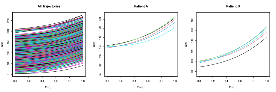
Figure 4: Quantile functions simulated from model (3) for $n=500$ study participants with a total of $2500$ visits ($J=5$ visits per person) and $\rho=0.3$. Left panel: all trajectories; Center and right panels: two study participants.

We analyze the results $\widehat{MSE}_{b}$ for $b=1,\ldots,B$ to determine two metrics:

$$\widehat{\mu}=\inf\left\{t\in\mathbb{R}:\widehat{F}(t)=\frac{1}{B}\sum_{b=1}^{B}\mathbb{I}(\widehat{MSE}_{b}\leq t)\geq 0.5\right\}$$

and

$$\widehat{\sigma}=\sqrt{\frac{1}{B}\sum_{b=1}^{B}\left(\widehat{MSE}_{b}-\widehat{\mu}\right)^{2}},$$

representing the median and standard deviation of the model’s performance. These metrics provide insights into the expected, worst, and best-case scenarios. Additionally, we define the squared bias for descriptive analysis as:

$${\rm Bias}^{2}=\left[\int_{0}^{1}\left(100+20p+20p^{2}+20p^{3}-\frac{1}{B}\sum_{b=1}^{B}\widehat{\beta}_{b,1}(p)\right)\,dp\right]^{2}\;.$$

$\rho=0.0$	$J=5$	$J=10$	$J=20$
$n=300$	$1.30$ $(4.47)$	$1.48$ $(4.49)$	$1.63$ $(3.96)$
$n=500$	$0.82$ $(2.49)$	$0.94$ $(2.33)$	$0.74$ $(2.58)$
$n=1000$	$0.40$ $(1.50)$	$0.48$ $(1.24)$	$0.35$ $(1.11)$
$n=2000$	$0.32$ $(0.74)$	$0.16$ $(0.69)$	$0.25$ $(0.65)$

$\rho=0.3$	$J=5$	$J=10$	$J=20$
$n=300$	$1.22$ $(4.47)$	$1.35$ $(4.08)$	$1.57$ $(4.80)$
$n=500$	$0.94$ $(2.72)$	$0.74$ $(2.56)$	$0.81$ $(2.37)$
$n=1000$	$0.38$ $(1.18)$	$0.35$ $(1.38)$	$0.42$ $(1.17)$
$n=2000$	$0.22$ $(0.74)$	$0.26$ $(0.53)$	$0.19$ $(0.63)$

$\rho=0.6$	$J=5$	$J=10$	$J=20$
$n=300$	$1.35$ $(4.22)$	$1.21$ $(3.41)$	$1.23$ $(5.49)$
$n=500$	$0.63$ $(2.02)$	$0.81$ $(2.61)$	$0.74$ $(2.51)$
$n=1000$	$0.42$ $(1.28)$	$0.42$ $(1.22)$	$0.34$ $(1.10)$
$n=2000$	$0.25$ $(0.77)$	$0.23$ $(0.58)$	$0.21$ $(0.73)$

Table 1: Median of $\widehat{MSE}_{b}$, $\widehat{\mu}$ over $b=1,\ldots,B$ and the associated standard deviation within brackets, $\widehat{\sigma}$. Results are organized by correlation coefficients ($\rho\in\{0,0.3,0.6\}$), sample sizes ($n\in\{300,500,1000,2000\}$), and number of visits ($J\in\{5,10,20\}$).

Table 1 presents the median $\widehat{\mu}$ and standard deviation $\widehat{\sigma}$ (in brackets) of $\widehat{MSE}_{b}$, organized by correlation coefficients ($\rho\in\{0,0.3,0.6\}$) and sample sizes ($n\in\{300,500,1000,2000\}$). The worst-case scenario in our bias analysis yields a bias of $0.12$, indicating a high degree of agreement among the models and near-unbiasedness of the fixed-effect estimator. Table 3 shows the coverage obtained in the $B=1000$ simulations for the joint and pointwise confidence bands for the simulation cases $J=5,\rho=0.3,\text{ and }n=300,500,1000,2000.$

	Type	Number of subjects
		300	500	1000	2000
	Coverage (Joint)	0.93	0.95	0.96	0.95
	Coverage (Pointwise)	0.94	0.96	0.95	0.94

Table 2: Table evaluating the coverage of our method. The study was conducted at a confidence level of 95% and across various sample sizes $n\in\{300,500,1000,2000\},$ $J=5$ and $\rho=0.3$. The results show that the coverage was satisfactory for all sample sizes tested.

Key findings from this simulation study include:

1. Increasing the sample size $n$ leads to a decrease in both the median, $\widehat{\mu}$, and standard deviation, $\widehat{\sigma}$, of the mean-square error.

2. The Mean Squared Error (MSE) demonstrates consistency across different simulations in terms of $\widehat{\mu}$ and $\widehat{\sigma}$ for various combinations of the correlation parameter, $\rho$, and the number of visits, $J$. This indicates the robustness of the models when dealing with correlations in the predictions. Additionally, our method exhibits computational efficiency as the number of visits increases, attributable to the pointwise nature of the proposed algorithm. This efficiency is achieved without sacrificing statistical effectiveness.

3. In our analysis, the function $\beta_{1}(\cdot)$ is identified with the estimation of the mean population glucose level. This estimation serves as a crucial summary metric, particularly for quantifying clinical differences between two groups in a clinical trial. We quantify the interval $\widehat{\mu}\pm 2\widehat{\sigma}$, which likely contains 95% of the measurement errors, to be approximately $\pm(1-12)\,\text{mg/dL}$ for glucose concentration. This provides a measure of uncertainty for the error estimations in $\beta_{1}(\cdot)$. Notably, this range is relatively small compared to the clinically relevant glucose levels, which typically range from $40$ to $600\,\text{mg/dL}$.

4. The coverage obtained using joint and pointwise methods for different sample sizes is very close to the nominal value, despite the shape constraints of the outcome quantile functions. These results indicate, in this intermediate case examined, the robustness of the bootstrap method in calibrating confidence bands in multi-level models that incorporate only a quantile-time dependet global mean as a fixed effect.

4.3 Direct simulation of the multilevel quantile process from a set of covariates

In line with the multilevel quantile generative model discussed in the previous section, this section presents a simulation study designed to assess multilevel functional outcomes. These outcomes are based on additional effects in the fixed-effect model component of the covariate set $\mathbf{X}$. These simulations are particularly relevant for Continuous Glucose Monitoring (CGM) clinical trials, where the metabolic response of patients is influenced by characteristics such as age, sex, baseline metabolic status, and anthropometric measures. Unlike previous simulation studies, we focus on the pointwise error across all probabilities $p\in[0,1]$, with the analysis centered on the functional coefficients $\beta_{l}(p),l=1,\ldots,L$, which are solely related to the patient characteristics $\mathbf{X}$. We denote by $\beta_{0}(p)$, the intercept.

For each participant $i$ in the study and each visit $j$, we simulate $n_{ij}$ quantile random processes $Q_{ij}(\cdot)$ by adding a term for the covariates $\mathbf{X}_{ij}$. The quantile process $Q_{ij}(p)$ is defined by the model:

$$Q_{ij}(p)=100+20(p+p^{2}+p^{3})+3p\left(\sum_{l=1}^{L}X_{ijl}\right)+U_{i}+\frac{10pjW_{ij}}{J}+\epsilon_{ij},$$ (4)

where $U_{i}$, $W_{ij}$, and $\epsilon_{ij}$ are mutually independent, each following a normal distribution $N(0,3^{2}),N(0,1),$ and $N(0,1)$, respectively.

For simplicity, we assume that the patient characteristics across visits are the same, i.e., $\mathbf{X}_{ij}=\mathbf{X}_{i}=(\mathbf{X}^{i1},\dots,\mathbf{X}^{iL})^{\top}$, and are modeled as independent uniform distributions, $\mathbf{X}^{il}\sim U(0,3)$, for each $l=1,\dots,L$.

For simplicity in the results description, we only focus on the scenarios with $n\in\{300,500,1000,2000\}$, $J\in\{10\}$, $L=\{1,3,5,10\}$, and $\epsilon_{ij}\sim N(0,1)$. Given the symmetric nature of the fixed effects $\beta_{l}(p)=3p$ for $l=1,\ldots,L$, for each simulation run $b=1,\ldots,B=1000$, we evaluate the model error performance using the pointwise MSE only in the first random covariate:

$$\widehat{MSE}_{b}(p)=\left\{3p-\widehat{\beta}_{b,1}(p)\right\}^{2}.$$ (5)

The results $\widehat{MSE}_{b}(p)$ for $b=1,\ldots,B$ are analyzed using the following metrics:

$$\widehat{\mu}(p) =\inf\left\{t\in\mathbb{R}:\widehat{F}(t)=\frac{1}{B}\sum_{b=1}^{B}\mathbb{I}(\widehat{MSE}_{b}(p)\leq t)\geq 0.5\right\},$$ (6)

$$\widehat{\sigma}(p) =\sqrt{\frac{1}{B}\sum_{b=1}^{B}\left(\widehat{MSE}_{b}(p)-\widehat{\mu}(p)\right)^{2}},$$ (7)

representing the median and standard deviation of the model’s performance, respectively.

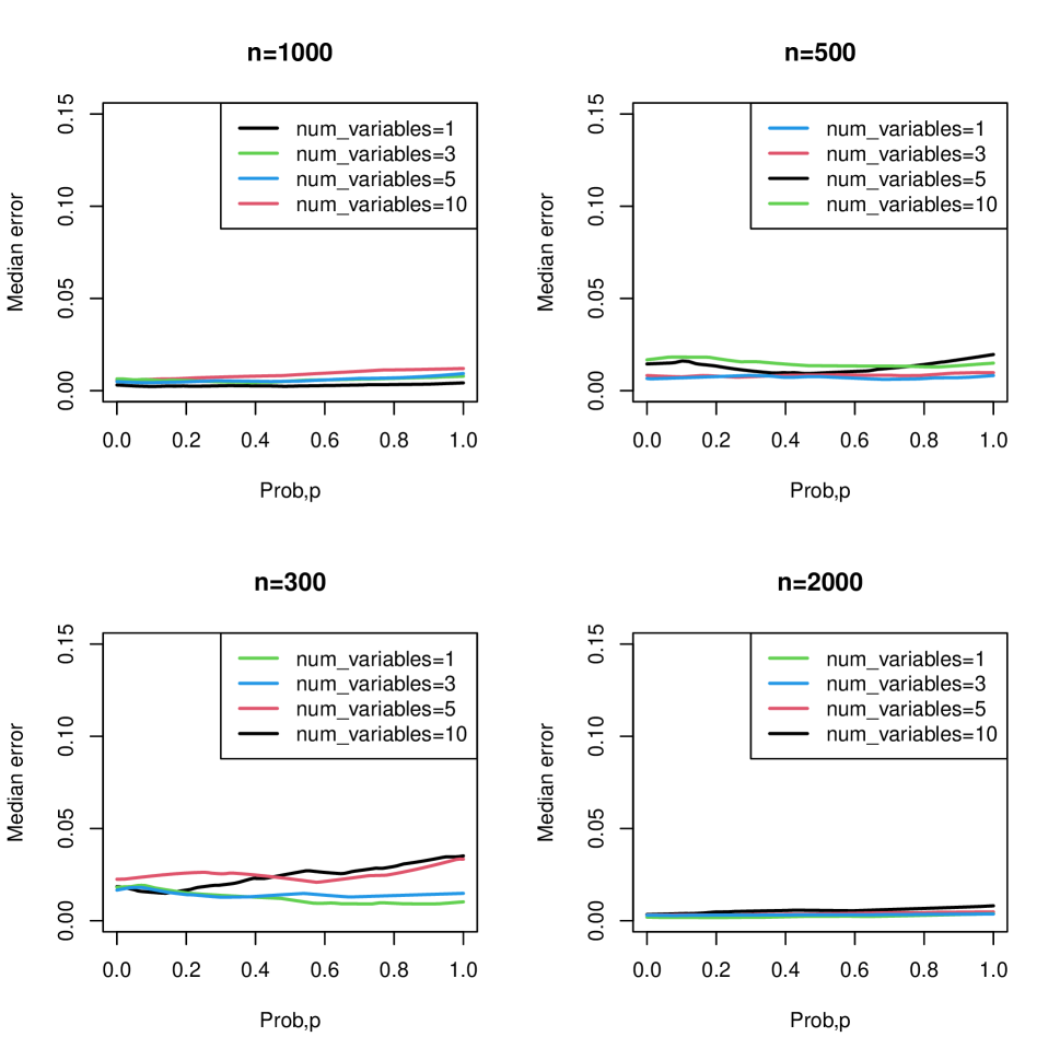
(a) Error $\widehat{\mu}(p)$.

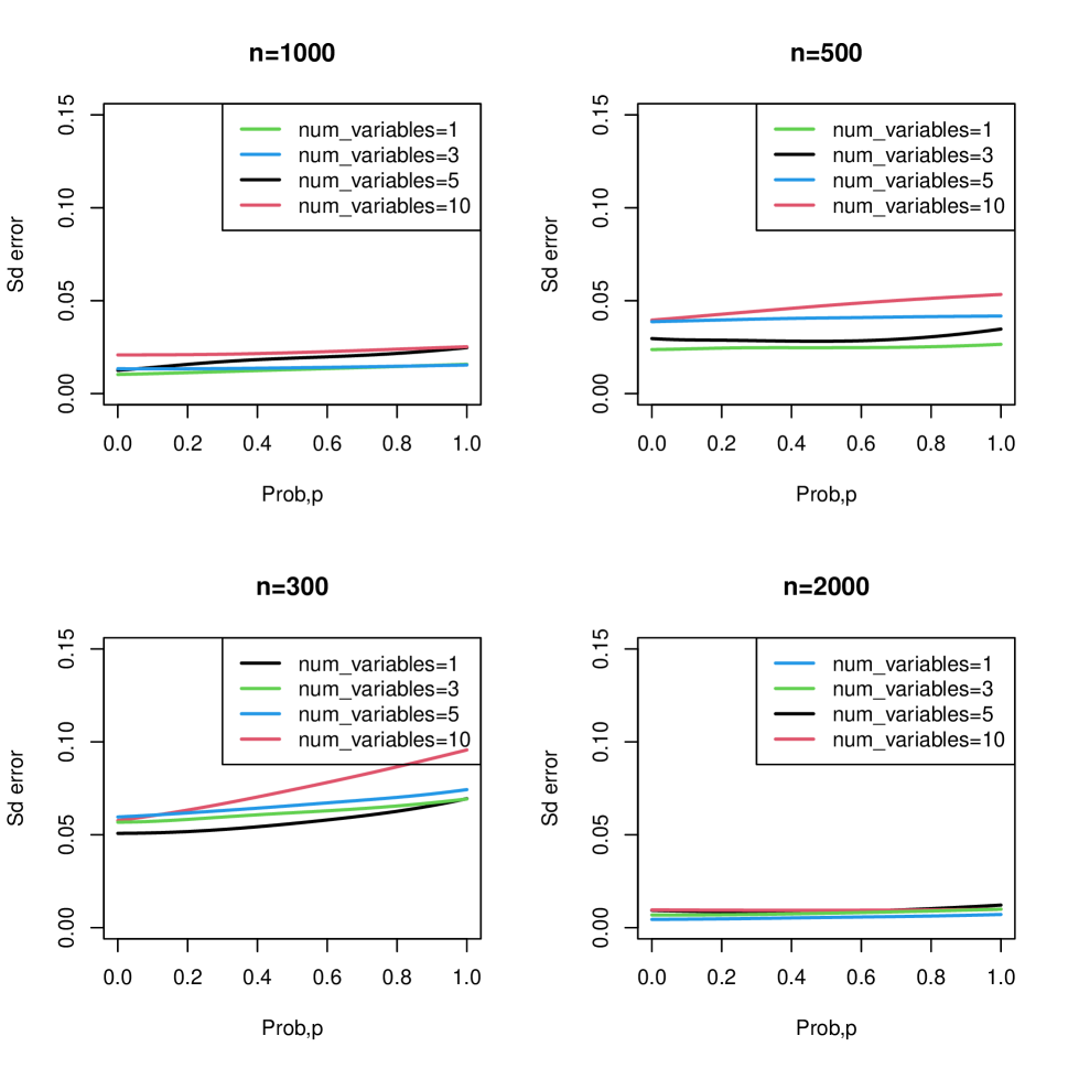
(b) Error $\widehat{\sigma}(p)$.

Figure 5: Median of $\widehat{MSE}_{b}(p)$, $\widehat{\mu}(p)$ over $b=1,\ldots,B$ and the associated standard deviation within brackets, $\widehat{\sigma}(p)$. Results are organized by sample sizes ($n\in\{300,500,1000,2000\}$), and a fixed number of visits ($J\in\{10\}$).

Figure 5 shows $\widehat{\mu}(p)$ and $\widehat{\sigma}(p)$. Interestingly, in cases of small sample size $n=300,500$, $\widehat{\sigma}(p)$ can dominate $\widehat{\mu}(p)$, especially when the dimension of the predictor is large, such as $L=10$. As the sample size increases, this effect vanishes across all $p\in[0,1]$, with the error magnitude becoming consistent.

	Type	Number of subjects
		300	500	1000	2000
	Coverage (Joint)	0.94	0.95	0.96	0.94
	Coverage (Pointwise)	0.93	0.95	0.96	0.95

Table 3: Table evaluating the coverage of our method. The study was conducted at a confidence level of 95% and across various sample sizes $n\in\{300,500,1000,2000\}$, $J=10$ and $L=5$. The results show that the coverage was satisfactory for all sample sizes tested.

Key findings from this simulation study include:

1. Increasing the sample size $n$ leads to a decrease in both the median, $\widehat{\mu}(p)$, and standard deviation, $\widehat{\sigma}(p)$, across all $p\in[0,1]$.

2. With an increase in the number of covariates in the model $L$, the error increases, as does the effect of the curse of dimensionality.

3. Generally, with the increase of probability $p\in[0,1]$, the error increases due to the variance of the random effect related to the individual-visit, increasing with $p$, which increases the overall effect of random effect estimation. In all cases with $n=2000$, the error is invariant to the quantile-probability in both location and scale metrics errors.

4. The coverage obtained using joint and pointwise methods for different sample sizes is very close to the nominal value, despite the shape constraints of the outcome quantile functions. These results indicate, in this intermediate case examined, the robustness of the bootstrap method in calibrating confidence bands in multi-level models that incorporate external covariates in the fixed-effects.

5 Results for the Juvenile Diabetes Research Foundation Continuous Glucose Monitoring Study Group

5.1 Scalar Multilevel functional model

Our analysis is founded on data obtained from the Juvenile Diabetes Research Foundation Continuous Glucose Monitoring Study Group, which is detailed in Section 2. Initially, we conducted a preliminary analysis using the mean glucose values obtained from CGM data during seven predefined periods as a scalar response variable. This initial step allowed us to gain insights into the information captured by traditional methods.

Subsequently, we compared these preliminary findings with results obtained using the new notion of glucodensity as a response, and incorporate the related quantile as random response in the multilevel functional model. Our principal scientific hyphotesis was to evaluate is the new models provide new findings in the clinical practice, surpassing the limitations of traditional methods and the lack of orientations to detect diferent distributional characteristics as quantiles.

The multilevel model employed for scalar-response, using mean glucose values, adheres to the following structure:

$$G_{ij}=\sum_{l=1}^{L}X_{ijl}\beta_{l}+U_{i0}+Z_{ij}U_{i}+W_{ij}.$$ (8)

In this equation, $G_{ij}$ represents the glucose sample mean for patient $i$ during period $j$. The term $X_{ijl}$ corresponds to $L$ fixed effects covariates, with $\beta_{l}$ as the corresponding fixed effect parameter. The term $U_{i0}$ accounts for individual intercept random effects, while $Z_{ij}$ is the random effects covariate associated with the time period, and $U_{i}$ represents the slope effect corresponding to subject $i$. The term $W_{ij}$ accounts for the residual variation that remains unexplained by the fixed or random effects. We assumed that the processes $U_{i0}$, $U_{i}$, and $W_{ij}$ were random errors, with $W_{ij}$ being uncorrelated with all $U_{i0}$ and $U_{i}$, although the intercept and slope random effects could be correlated with each other.

The model was fitted with $L=11$ fixed effects, including an intercept and ten covariates: RT-CGM (a binary variable indicating whether an individual utilizes a CGM device for glucose control, taking a value of 1 if yes and 0 otherwise), sex (male/female), weight, age, pump, period of the year (with one reference category and four factor variables), and HbA1c. Each variable’s effect, $\beta_{l}$, represents the association between the fixed predictor and the conditional mean predictor, assuming a linear association.

Additionally, our model included random intercept and slope terms to account for individual and subject-visit variability in the prediction of conditional glucose mean values. These components play a crucial role in understanding the underlying biological variations factors at individual and visit level. However, our primary focus in this paper is to study the longitudinal statistical associations, between the clinical outcome, $G_{ij}$, and the fixed-effects, $X_{ijp}$.

Variable Name	Description
Age	Age in years of the participant at the time of screening.
Group	Binary variable indicating if the patient belongs to the control or treatment group (RT-CGM).
Weight	Weight (kg).
Gender	Binary variable indicating the gender of the patient.
HbA1c	Baseline glycosylated hemoglobin variable.
Pump	Binary variable indicating if the patient follows insulin therapy with insulin pump or injections.
Seasonal	• Level 1: First seven weeks of the year. • Level 2: Weeks 7-17. • Level 3: Weeks 18-33. • Level 4: Weeks 33-39. • Level 5: Rest of the year.
ID	Identification number of the patient.
Visit	Visit number of the patient.

Table 4: Description of the variables used in the Juvenile Diabetes Research Foundation Continuous Glucose Monitoring Study Group.

Variable Name	Estimation Value (CI 95%)	p-value	Standardised Estimates
Intercept	80.18 (60.87–99.7)	$<0.001$
RT-CGM	-5.47 (-9.06–1.88)	0.03215	-5.47
Male	-2.60 (-6.17-0.96)	0.15	-2.60
Weight	-0.063 (-0.17-0.04)	0.23	-0.0459
Age	-0.46 (-0.59–0.34)	$<0.001$	-0.2739
Pump	-7.96 (-12.61–3.32)	$<0.001$	-7.96
Seasonal_2	-1.38 (-3.43-0.66)	0.18	-1.38
Seasonal_3	-0.64 (-2.63-1.35)	0.52	-0.64
Seasonal_4	0.038 (-2.28-2.36)	0.97	0.038
Seasonal_5	0.101 (-1.71-1.92)	0.90	0.101
HbA1c	14.7 (12.50-16.93)	$<0.001$	0.4463

Table 5: $\beta$-coefficients for the fixed-terms of numerical and categorical predictors in the estimation of the conditional mean for scalar glucose CGM mean. Conditional R-square equal to 0.72. Marginal R-square equal to 0.35.

Table 4 offers a concise summary of the scalar variables utilized in our analysis, along with their respective clinical significance. For comparison, we present the results of a traditional analysis based on mean glucose estimates derived from CGM in Table 5. The marginal R-squared values for most variables, with the exceptions of HbA1c (0.18) and Age (0.05), demonstrate relatively low explanatory power, leading to a total marginal R-squared value of 0.35 when considering all fixed effects. It is evident that these variables, on their own, only account for a moderate proportion of the overall variation in glucose responses. However, when considering the impact of random effects, the conditional R-squared increases significantly to 0.72. This notable increase in the conditional R-squared underscores the substantial contribution of random effects in explaining the variability in patient responses to the intervention.

The variables with the largest absolute coefficients are HbA1c, Pump, and RT-CGM, indicating their significant association with mean glucose values. Age also plays a significant role, as evident from the normalized coefficients, statistical significance, and marginal R-squared. Generally, an increase in age corresponds to a reduction in mean glucose values, while higher HbA1c levels elevate mean glucose values. Additionally, the use of CGM values (RT-CGM) is associated with lower glucose values. On the other hand, gender and seasonal variables do not exhibit statistical significance, suggesting minimal impact, similar to the weight of an individual patient at least in the average glucose values of the CGM time series.

5.2 Distributional Multilevel Functional model

In this section, our attention shifts towards the distributional functional model, where we employ the equation (2) with $L=11$ fixed effects. These fixed effects comprise an intercept and ten covariates, as elaborated in Table 4, maintaining consistency with the scalar response multilevel models. To capture the impact of each variable, $\beta_{l}(p)$, we adopt an unspecified nonparametric function of the probability $p$.

Our model also included a random intercept and slope, with $K=2$, $Z_{ij1}=1$, and $Z_{ij2}=j$ for every $i=1,\ldots,I$ and $j=1,\ldots,J_{i}$. The functional random intercept and slope, $U_{i1}(p)$ and $U_{i2}(p)$, were allowed to be correlated across probabilities $p$ but were assumed to be independent across subjects $i$. The subject/period-specific deviations $W_{ij}(p)$ were unspecified across $p$ but were assumed to be independent across $i$ and $j$ and mutually independent of $U_{i1}(p)$ and $U_{i2}(p)$, respectively. This random effects structure is similar to the LFPCA structure in Greven et al. (2010).

As outlined in Greven et al. (2010), the analysis of random functional effects allows us to quantify the variability associated with subjects’ baseline quantile functions, differences in subjects’ average changes over time, visit-specific variation around subject-specific trends, and measurement error. Through longitudinal functional principal component analysis (LFPCA), we obtain scores on various components, enabling investigation of potential latent subgroups or associations with covariates or health outcomes. Furthermore, the functional principal components provide insights into the data structure and the dimensionality of underlying lower-dimensional spaces that explain observed variability, akin to the associations of predictors with the clinical outcome within the multilevel model.

Nonetheless, the primary focus of this paper is to study the probability-dependent associations between the fixed effects, $X_{ijp}$, and the longitudinally observed quantile curves, $Q_{ij}(p)$. While acknowledging the LFPCA structure of random effects, as it significantly affects inference and the calculation of confidence intervals and p-values for the coefficients $\beta_{p}(\cdot)$, $p=1,\ldots,L$, we can focus only in the fixed-effect analysis.

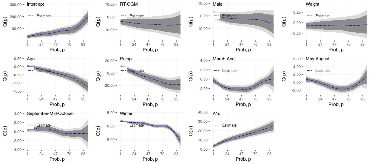
Figure 6: $\beta-$ functional coefficients for the fixed-terms of numerical and categorical predictors in the estimation of the conditional mean for the distributional quantile representation

Bellow, we fitted Model (2) using the FUI approach described in Section 3.2. Figure 6 presents the estimated functional coefficient estimates, along with pointwise unadjusted confidence intervals (dark shade of gray) and correlation and multiplicity adjusted confidence intervals (lighter shade of gray) Crainiceanu et al. (2024).

To interpret the results, it is important to note that smaller probabilities correspond to lower quantiles, representing the hypoglycemic range. Conversely, larger probabilities correspond to higher quantiles, representing the hyperglycemic range. Figure 6 presents a large number of results that require careful and sequential analysis.

We start by examining the panel corresponding to the RT-CGM variable (indicator of the treatment group) in the first row, second column. The point estimator consistently shows a negative value, indicating a reduction in blood glucose levels across all quantile levels. The reduction is more pronounced in the hyperglycemic ranges, as indicated by the decreasing values of $\widehat{\beta}_{2}(p)$ with increasing values of $p$. However, these reductions were not statistically significant for quantiles corresponding to $p<0.20$, when considering the joint confidence intervals. For higher quantiles, the reductions are significant, though the confidence intervals are very close to covering $0$.

Moving on to the third and fourth panels in the first row of Figure 6, these correspond to the effects of sex and weight on blood glucose levels at all values. The results indicate that the effects of these variables are not statistically distinguishable from zero (light shaded areas contain zero for every value of $p$). These estimates are conditional on several other covariates, including treatment group, baseline HbA1c, and age.

In the second row, the first panel corresponds to age, showing a highly significant effect, particularly in the hyperglycemic range, indicating better glycemic control for older individuals. The second panel in this row focuses on the use of an insulin pump, indicating that its use was not statistically significant in the lower glycemic range but was strongly statistically significant in terms of reducing blood glucose levels in the hyperglycemic range.

The third and fourth panels in the second row, as well as the first and second panels in the third row, display results for different times of the year relative to the reference period comprising the first seven weeks of the year. These results indicate strong, statistically significant effects of various periods of the year on blood glucose levels. If confirmed, these differences could provide valuable insights into the natural annual variations in glycemic control that should be considered in clinical decision-making and research applications.

The third panel in the third row of Figure 6 corresponds to the association between baseline HbA1c and measured CGM. The results indicate a very strong and statistically significant association across all quantile levels. The effect of HbA1c on CGM measurements increases linearly across all quantiles (probabilities). The lowest effect was found in the hypoglycemic range, where an increase of $1$ unit in HbA1c was estimated to be associated with an average increase of $7$mg/dL in the lowest quantile ($p=0.01$) and an average increase of $20$mg/dL in the highest quantile ($p=0.99$). While not directly comparable, the estimated effect in Table 4 provides an estimate of $14.7$mg/dL in average blood glucose over the day, as measured by CGM, for each increase of one unit in HbA1c. This analysis is also in line with an analysis of median CGM, which would provide an estimate of $15.0$mg/dL. These results suggest that the association between HbA1c and daily trajectories of CGM is more complex and not completely captured by taking the mean CGM over the day.

Our analysis complements the original findings Tamborlane et al. (2008); Juvenile Diabetes Research Foundation Continuous Glucose Monitoring Study Group (2009) by (1) providing results across the entire blood glucose range while accounting for covariates and the longitudinal structure of the data, (2) accounting for variables such as insulin pump use that were not balanced by random treatment assignment, and (3) quantifying the seasonal variations of blood glucose for the first time. In particular, our implementation of the new distributional method has yielded compelling evidence that age plays a pivotal role in glycemic control, extending beyond the conventional analysis of mean glucose values. Our findings also demonstrate the effectiveness of Continuous Glucose Monitoring (CGM) in enhancing glycemic control, particularly in the higher probabilities of the quantile function, and its significance in the hyperglycemia range. We have identified a linear association between HbA1c levels and all quantile functions, that is a new clinical result in a CGM litereture. Most of the litereture focus on the connection of the HbA1c levels with the CGM glucose mean values, and the glucose variability, but no with the CGM quantile functions that are related explicity with CGM time in range metrics. Additionally, we have observed variations in glucose distribution across different seasonal periods, with a more pronounced effect during winter. However, we found no significant effects related to sex and weight in glycemic variations, suggesting a high degree of heterogeneity in patient responses to these factors. Maybe, in another elderly populations, in which, there are a lost of functional capacity of the patients, the effects are more evident.

From a methodological standpoint, our novel multilevel model offers significant advantages over traditional multilevel algorithms. The new method provides a comprehensive and insightful description of the longitudinal evolution of distributional characteristics of CGM time series over a four-week period, while effectively accounting for patient characteristics. This allows us to gain a deeper understanding of how the distributional characteristics of CGM data change over time for each patient, while mitigating the potential impact of confounders.

6 Discussion

This paper introduces a novel approach to analyze wearable data within the context of clinical trials. Our method leverages distributional representations and employs a multilevel functional regression model for distributions. We contend that this type of data structures will continue to increase in the future and that theer will be increased interest in: (1) summarizing high-dimensional functional data as distributions; and (2) modeling the known multilevel or longitudinal data structure of the resulting distributions. In this paper we focused on the quantile function of glucose profiles derived from Continuous Glucose Monitoring (CGM) technology.

Our methods are complementary to the multilevel functional methodology proposed by Gaynanova et al. (2022) and Sergazinov et al. (2023). However, these methods focused on analyzing glucose fluctuations from sleep onset, a period of the day that is not subject to food intake and physical activity. Therefore, these methods cannot be directly extended to CGM during the day because of the heterogeneity of the various events that influence CGM measurements. For these reasons we replaced the CGM time series over multiple weeks with the distribution of the CGM measurements over that period. The downside is that we loose the time-dependence within the four week period, but we gain in interpretability of the CGM measurements during real-life, free-living conditions.

References

- (1)
-
Ajjan (2017)
Ajjan, R. A. (2017), ‘How can we realize the clinical benefits of continuous glucose monitoring?’, Diabetes technology & therapeutics 19(S2), S27–S36.
28541132[pmid].
https://pubmed.ncbi.nlm.nih.gov/28541132 -
Ajjan et al. (2019)
Ajjan, R., Slattery, D. & Wright, E. (2019), ‘Continuous glucose monitoring: A brief review for primary care practitioners’, Advances in Therapy 36(3), 579–596.
https://doi.org/10.1007/s12325-019-0870-x -
Bailey et al. (2015)
Bailey, T., Bode, B. W., Christiansen, M. P., Klaff, L. J. & Alva, S. (2015), ‘The performance and usability of a factory-calibrated flash glucose monitoring system’, Diabetes Technology & Therapeutics 17(11), 787–794.
PMID: 26171659.
https://doi.org/10.1089/dia.2014.0378 - Battelino et al. (2022) Battelino, T., Alexander, C. M., Amiel, S. A., Arreaza-Rubin, G., Beck, R. W., Bergenstal, R. M., Buckingham, B. A., Carroll, J., Ceriello, A., Chow, E. et al. (2022), ‘Continuous glucose monitoring and metrics for clinical trials: an international consensus statement’, The Lancet Diabetes & Endocrinology .
-
Beck et al. (2018)
Beck, R. W., Bergenstal, R. M., Riddlesworth, T. D., Kollman, C., Li, Z., Brown, A. S. & Close, K. L. (2018), ‘Validation of Time in Range as an Outcome Measure for Diabetes Clinical Trials’, Diabetes Care 42(3), 400–405.
https://doi.org/10.2337/dc18-1444 -
Beck et al. (2012)
Beck, R. W., Calhoun, P. & Kollman, C. (2012), ‘Use of continuous glucose monitoring as an outcome measure in clinical trials’, Diabetes Technology & Therapeutics 14(10), 877–882.
PMID: 23013201.
https://doi.org/10.1089/dia.2012.0079 - Ben-Yacov et al. (2021) Ben-Yacov, O., Godneva, A., Rein, M., Shilo, S., Kolobkov, D., Koren, N., Cohen Dolev, N., Travinsky Shmul, T., Wolf, B. C., Kosower, N. et al. (2021), ‘Personalized postprandial glucose response–targeting diet versus mediterranean diet for glycemic control in prediabetes’, Diabetes care 44(9), 1980–1991.
- Brito & Dias (2022) Brito, P. & Dias, S. (2022), Analysis of Distributional Data, CRC Press.
-
Burge et al. (2008)
Burge, M. R., Mitchell, S., Sawyer, A. & Schade, D. S. (2008), ‘Continuous Glucose Monitoring: The Future of Diabetes Management’, Diabetes Spectrum 21(2), 112–119.
https://doi.org/10.2337/diaspect.21.2.112 - Crainiceanu et al. (2024) Crainiceanu, C., Goldsmith, J., Leroux, A. & Cui, E. (2024), Functional Data Analysis with R, Chapman and Hall/CRC.
- Cui et al. (2023) Cui, E. H., Goldfine, A., Quinlan, M., James, D. & Sverdlov, O. (2023), ‘Investigating the value of glucodensity analysis of continuous glucose monitoring data in type 1 diabetes: An exploratory analysis’, Frontiers in Clinical Diabetes and Healthcare 4, 1244613.
- Cui et al. (2021) Cui, E., Leroux, A., Smirnova, E. & Crainiceanu, C. M. (2021), ‘Fast univariate inference for longitudinal functional models’, Journal of Computational and Graphical Statistics pp. 1–12.
- Cui et al. (2022) Cui, E., Li, R., Crainiceanu, C. M. & Xiao, L. (2022), ‘Fast multilevel functional principal component analysis’, Journal of Computational and Graphical Statistics 0(0), 1–12.
- Di et al. (2009) Di, C.-Z., Crainiceanu, C. M., Caffo, B. S. & Punjabi, N. M. (2009), ‘Multilevel functional principal component analysis’, The annals of applied statistics 3(1), 458.
- Gaynanova et al. (2020) Gaynanova, I., Punjabi, N. & Crainiceanu, C. (2020), ‘Modeling continuous glucose monitoring (CGM) data during sleep’, Biostatistics .
- Gaynanova et al. (2022) Gaynanova, I., Punjabi, N. & Crainiceanu, C. (2022), ‘Modeling continuous glucose monitoring (cgm) data during sleep’, Biostatistics 23(1), 223–239.
-
Gertheiss et al. (2013)
Gertheiss, J., Goldsmith, J., Crainiceanu, C. & Greven, S. (2013), ‘Longitudinal scalar-on-functions regression with application to tractography data’, Biostatistics 14(3), 447–461.
https://doi.org/10.1093/biostatistics/kxs051 - Ghosal, Matabuena, Meiring & Petersen (2023) Ghosal, A., Matabuena, M., Meiring, W. & Petersen, A. (2023), ‘Predicting distributional profiles of physical activity in the nhanes database using a partially linear single-index fr’echet regression model’, arXiv preprint arXiv:2302.07692 .
-
Ghosal, Ghosh, Urbanek, Schrack & Zipunnikov (2023)
Ghosal, R., Ghosh, S., Urbanek, J., Schrack, J. A. & Zipunnikov, V. (2023), ‘Shape-constrained estimation in functional regression with bernstein polynomials’, Computational Statistics & Data Analysis 178, 107614.
https://www.sciencedirect.com/science/article/pii/S0167947322001943 - Ghosal & Matabuena (2023) Ghosal, R. & Matabuena, M. (2023), ‘Multivariate scalar on multidimensional distribution regression’, arXiv preprint arXiv:2310.10494 .
- Ghosal, Varma, Volfson, Hillel, Urbanek, Hausdorff, Watts & Zipunnikov (2021) Ghosal, R., Varma, V. R., Volfson, D., Hillel, I., Urbanek, J., Hausdorff, J. M., Watts, A. & Zipunnikov, V. (2021), ‘Distributional data analysis via quantile functions and its application to modelling digital biomarkers of gait in alzheimer’s disease’.
- Ghosal, Varma, Volfson, Urbanek, Hausdorff, Watts & Zipunnikov (2021) Ghosal, R., Varma, V. R., Volfson, D., Urbanek, J., Hausdorff, J. M., Watts, A. & Zipunnikov, V. (2021), ‘Scalar on time-by-distribution regression and its application for modelling associations between daily-living physical activity and cognitive functions in alzheimer’s disease’.
- Goldsmith et al. (2012) Goldsmith, A., Crainiceanu, C., Caffo, B. & Reich, D. (2012), ‘Longitudinal penalized functional regression for cognitive outcomes on neuronal tract measurements’, Journal of Royal Statistical Society Series C Applied Statistics 61(3), 453–469.
-
Goldsmith et al. (2020)
Goldsmith, J., Scheipl, F., Huang, L., Wrobel, J., Di, C., Gellar, J., Harezlak, J., McLean, M., Swihart, B., Xiao, L., Crainiceanu, C. & Reiss, P. (2020), refund: Regression with Functional Data.
R package version 0.1-23.
https://CRAN.R-project.org/package=refund -
Greven et al. (2010)
Greven, S., Crainiceanu, C., Caffo, B. & Reich, D. (2010), ‘Longitudinal functional principal component analysis’, Electronic journal of statistics 4, 1022–1054.
21743825[pmid].
https://pubmed.ncbi.nlm.nih.gov/21743825 - Juvenile Diabetes Research Foundation Continuous Glucose Monitoring Study Group (2009) Juvenile Diabetes Research Foundation Continuous Glucose Monitoring Study Group, T. (2009), ‘The effect of continuous glucose monitoring in well-controlled type 1 diabetes’, Diabetes care 32(8), 1378–1383.
- Koffman et al. (2023) Koffman, L., Crainiceanu, C. & Leroux, A. (2023), ‘Walking fingerprinting’, arXiv preprint arXiv:2309.09897 .
- Leshem et al. (2020) Leshem, A., Segal, E. & Elinav, E. (2020), ‘The gut microbiome and individual-specific responses to diet’, Msystems 5(5), e00665–20.
- Liao et al. (2019) Liao, Y., Thompson, C., Peterson, S., Mandrola, J. & Beg, M. S. (2019), ‘The future of wearable technologies and remote monitoring in health care’, American Society of Clinical Oncology Educational Book 39, 115–121.
- Martens et al. (2021) Martens, T. W., Bergenstal, R. M., Pearson, T., Carlson, A. L., Scheiner, G., Carlos, C., Liao, B., Syring, K. & Pollom, R. D. (2021), ‘Making sense of glucose metrics in diabetes: linkage between postprandial glucose (ppg), time in range (tir) & hemoglobin a1c (a1c)’, Postgraduate Medicine 133(3), 253–264.
- Matabuena et al. (2023) Matabuena, M., Félix, P., Ditzhaus, M., Vidal, J. & Gude, F. (2023), ‘Hypothesis testing for matched pairs with missing data by maximum mean discrepancy: An application to continuous glucose monitoring’, The American Statistician pp. 1–13.
- Matabuena, Felix, Garcia-Meixide & Gude (2022) Matabuena, M., Felix, P., Garcia-Meixide, C. & Gude, F. (2022), ‘Kernel machine learning methods to handle missing responses with complex predictors. application in modelling five-year glucose changes using distributional representations’, Computer Methods and Programs in Biomedicine 221, 106905.
-
Matabuena, Félix, Hammouri, Mota & del Pozo Cruz (2022)
Matabuena, M., Félix, P., Hammouri, Z. A. A., Mota, J. & del Pozo Cruz, B. (2022), ‘Physical activity phenotypes and mortality in older adults: a novel distributional data analysis of accelerometry in the nhanes’, Aging Clinical and Experimental Research .
https://doi.org/10.1007/s40520-022-02260-3 - Matabuena, Karas, Riazati, Caplan & Hayes (2022) Matabuena, M., Karas, M., Riazati, S., Caplan, N. & Hayes, P. R. (2022), ‘Estimating knee movement patterns of recreational runners across training sessions using multilevel functional regression models’, The American Statistician (just-accepted), 1–24.
-
Matabuena & Petersen (2023)
Matabuena, M. & Petersen, A. (2023), ‘Distributional data analysis of accelerometer data from the NHANES database using nonparametric survey regression models’, Journal of the Royal Statistical Society Series C: Applied Statistics 72(2), 294–313.
https://doi.org/10.1093/jrsssc/qlad007 - Matabuena et al. (2021a) Matabuena, M., Petersen, A., Vidal, J. C. & Gude, F. (2021a), ‘Glucodensities: a new representation of glucose profiles using distributional data analysis’, Statistical methods in medical research .
- Matabuena et al. (2021b) Matabuena, M., Petersen, A., Vidal, J. C. & Gude, F. (2021b), ‘Glucodensities: a new representation of glucose profiles using distributional data analysis’, Statistical Methods in Medical Research 30(6), 1445–1464.
-
Nørgaard et al. (2023)
Nørgaard, K., Ranjan, A. G., Laugesen, C., Tidemand, K. G., Green, A., Selmer, C., Svensson, J., Andersen, H. U., Vistisen, D. & Carstensen, B. (2023), ‘Glucose Monitoring Metrics in Individuals With Type 1 Diabetes Using Different Treatment Modalities: A Real-World Observational Study’, Diabetes Care p. dc231137.
https://doi.org/10.2337/dc23-1137 - Petersen et al. (2021) Petersen, A., Liu, X. & Divani, A. A. (2021), ‘Wasserstein -tests and confidence bands for the fréchet regression of density response curves’, The Annals of Statistics 49(1), 590–611.
- Reiss et al. (2010) Reiss, P., Huang, L. & Mennes, M. (2010), ‘Fast function-on-scalar regression with penalized basis expansions’, International Journal of Biostatistics 6, 1.
-
Rodbard (2016)
Rodbard, D. (2016), ‘Continuous glucose monitoring: A review of successes, challenges, and opportunities’, Diabetes Technology & Therapeutics 18(S2), S2–3–S2–13.
PMID: 26784127.
https://doi.org/10.1089/dia.2015.0417 -
Rodbard (2017)
Rodbard, D. (2017), ‘Continuous glucose monitoring: A review of recent studies demonstrating improved glycemic outcomes’, Diabetes Technology & Therapeutics 19(S3), S–25–S–37.
PMID: 28585879.
https://doi.org/10.1089/dia.2017.0035 - Scheipl et al. (2015) Scheipl, F., Staicu, A.-M. & Greven, S. (2015), ‘Functional additive mixed models’, Journal of Computational and Graphical Statistics 24(2), 477–501.
-
Schnell et al. (2017)
Schnell, O., Barnard, K., Bergenstal, R., Bosi, E., Garg, S., Guerci, B., Haak, T., Hirsch, I. B., Ji, L., Joshi, S. R., Kamp, M., Laffel, L., Mathieu, C., Polonsky, W. H., Snoek, F. & Home, P. (2017), ‘Role of continuous glucose monitoring in clinical trials: Recommendations on reporting’, Diabetes technology & therapeutics 19(7), 391–399.
28530490[pmid].
https://pubmed.ncbi.nlm.nih.gov/28530490 -
Sergazinov et al. (2023)
Sergazinov, R., Leroux, A., Cui, E., Crainiceanu, C., Aurora, R. N., Punjabi, N. M. & Gaynanova, I. (2023), ‘A case study of glucose levels during sleep using multilevel fast function on scalar regression inference’, Biometrics 79(4), 3873–3882.
https://onlinelibrary.wiley.com/doi/abs/10.1111/biom.13878 - Shou et al. (2015) Shou, H., Zipunnikov, V., Crainiceanu, C. M. & Greven, S. (2015), ‘Structured functional principal component analysis’, Biometrics 71(1), 247–257.
-
Staicu et al. (2010)
Staicu, A.-M., Crainiceanu, C. M. & Carroll, R. J. (2010), ‘Fast methods for spatially correlated multilevel functional data’, Biostatistics 11(2), 177–194.
https://doi.org/10.1093/biostatistics/kxp058 - Tamborlane et al. (2008) Tamborlane, W., Beck, R., Bode, B. et al. (2008), ‘Continuous glucose monitoring and intensive treatment of type 1 diabetes’, New England Journal of Medicine 359(14), 1464–1476.
- Tang et al. (2020) Tang, B., Zhao, Y., Venkataraman, A., Tsapkini, K., Lindquist, M. A., Pekar, J. & Caffo, B. (2020), ‘Differences in functional connectivity distribution after transcranial direct-current stimulation: a connectivity density point of view’, bioRxiv .
-
Wood et al. (2018)
Wood, A., O’Neal, D., Furler, J. & Ekinci, E. I. (2018), ‘Continuous glucose monitoring: a review of the evidence, opportunities for future use and ongoing challenges’, Internal Medicine Journal 48(5), 499–508.
https://onlinelibrary.wiley.com/doi/abs/10.1111/imj.13770 - Yoo & Kim (2020) Yoo, J. H. & Kim, J. H. (2020), ‘Time in range from continuous glucose monitoring: a novel metric for glycemic control’, Diabetes & metabolism journal 44(6), 828–839.
- Zipunnikov et al. (2014) Zipunnikov, V., Greven, S., Shou, H., Caffo, B., Reich, D. S. & Crainiceanu, C. (2014), ‘Longitudinal high-dimensional principal components analysis with application to diffusion tensor imaging of multiple sclerosis’, The annals of applied statistics 8(4), 2175.