Critical Fluctuations at Finite-Time Dynamical Phase Transition

We explore the critical properties of the recently discovered finite-time dynamical phase transition in the non-equilibrium relaxation of Ising magnets. The transition is characterized by a sudden switch in the relaxation dynamics and it occurs at a sharp critical time. While previous works have focused either on mean-field interactions or on investigating the properties of the critical time, we analyze the critical fluctuations at the phase transition in the nearest-neighbor Ising model on a square lattice using Monte Carlo simulations. By means of a finite-size scaling analysis, we extract the critical exponents for the transition. In two spatial dimensions, the exponents are consistent with those of the two-dimensional Ising universality class.

I Introduction

Non-equilibrium phase transitions are common across a wide range of disciplines in science [1], ranging from biological systems to galactic patterns. Their non-equilibrium nature allows these transitions to manifest themselves in a rich variety of both static and dynamic patterns [2]. Equilibrium phase transitions, by contrast, are more limited in regard to the possible ways in which they may occur. Furthermore, universality, a common property of equilibrium phase transitions, constrains the critical properties of phase transitions at equilibrium. As a consequence of these restrictions, equilibrium phase transitions are theoretically tractable and are nowadays comprehensively understood within the theory of equilibrium statistical mechanics [3, 4]. Similarly, near-equilibrium systems are in the realm of powerful theoretical frameworks, such as linear-response theory, that build upon the equilibrium theory.

Far from equilibrium, no theory of comparable scope is known and although some equilibrium methods can be generalized to far-from equilibrium [5, 6], the lack of an overarching theory makes the study of non-equilibrium phase transitions challenging.

Far-from-equilibrium thermal relaxation is a prime example of a genuine non-equilibrium process. As such, it exhibits a number of anomalous features, including ergodicity breaking [7], the Mpemba [8, 9] and Kovacs effects [10, 11, 12], and asymmetries associated with heating and cooling processes [13, 14, 15]. These anomalous phenomena are typically discussed in connection to an associated equilibrium phase transition [16].

Recent studies [17, 18, 19] revealed anomalous behavior in the extreme-event statistics of non-equilibrium relaxation in Ising magnets, namely, so-called finite-time dynamical phase transitions. These transitions manifest themselves through the emergence of kinks in the large-deviation (rate) functions of thermodynamic observables within the Curie-Weiss model of $N$ globally coupled Ising spins [17, 18] – see also the mathematical works in Refs. [20, 21, 22, 23]. The transitions occur during the transient relaxation following an instantaneous quench from the ferromagnetic phase into the paramagnetic phase of the model. Remarkably, many key features of this non-equilibrium transition are identical to the equilibrium phase transition of the Curie-Weiss model, including its (mean-field) critical exponents [17, 18]. Some effort has been made to explore this transition to models with short-range interactions [19]. So far, however, these studies have focused on accurately determining the transition time.

Here, we investigate critical phenomena associated with the finite-time dynamical phase transition in an Ising model with nearest-neighbor interactions on a two-dimensional square lattice with periodic boundary conditions. Although we do not expect equilibrium-like universality, categorizing critical fluctuations close to non-equilibrium phase transitions in terms of their critical exponents helps to characterize these transitions [24, 25, 26]. In some systems that exhibit both equilibrium and non-equilibrium phase transitions, the critical properties of the non-equilibrium transitions have been shown to fall in same universality class as the corresponding equilibrium transitions [26], leading to interesting correspondences between equilibrium and non-equilibrium.

Using a finite-size scaling analysis [27], we calculate the critical exponents associated with the magnetization and the magnetic susceptibility and show that their values are consistent with those of the two-dimensional Ising universality class at equilibrium. This provides further evidence that, akin to the mean-field model, critical properties of finite-time dynamical phase transitions in short-range models are identical to those of its equilibrium counterpart.

The paper is organized as follows: In Section II, we discuss the model and our methodology, and explain them by reviewing the well-known equilibrium phase transition in the two-dimensional Ising model. We also review the occurrence of the finite-time dynamical phase transitions in the mean-field version of the model. In Section III, we present our main results characterizing the critical properties of the nearest-neighbor Ising model. We draw our conclusions in the final Section IV of the paper.

II Background

In this Section, we introduce the model and discuss its equilibrium properties and how to treat finite-size effects. Subsequently, we review the origin of the finite-time dynamical phase transition in the mean-field version of the model [17, 18].

II.1 Model

We explore the critical properties of the finite-time dynamical phase transition for the nearest-neighbor Ising model (NNIM) on a two-dimensional square lattice with periodic boundary conditions. The internal energy of the model at vanishing external magnetic field reads

$$E=-J\sum_{\langle ij\rangle}S_{i}S_{j}\,,$$ (1)

where $J>0$ is the ferromagnetic nearest-neighbor coupling and $S_{i}=\pm 1$ denotes the state of the Ising spin at lattice site $i=1,\ldots,N$. The sum in Eq. (1) runs over all pairs of nearest neighbors.

In the mean-field version of the model, briefly discussed in Sec. II.6, one sums over all lattice sites (instead of nearest neighbors) and the coupling $J$ is scaled with the number $N$ of spins [28].

The system is immersed in a heat bath at inverse temperature $1/(k_{B}T)$. At equilibrium, the NNIM exhibits a second-order phase transition from a disordered into an ordered phase as a function of the so-called inverse coupling temperature,

$$\mathscr{J}\equiv J/(k_{B}T)\,.$$ (2)

The transition occurs at the critical value $\mathscr{J}_{c}\equiv J/(k_{B}T_{c})$, where $T_{c}$ denotes the Curie temperature. For the two-dimensional NNIM the value of $\mathscr{J}_{c}$ is given by [29]

$$\mathscr{J}_{c}=\frac{\ln(1+\sqrt{2})}{2}\approx 0.44\,,$$ (3)

while it is equal to unity in the mean-field version of the model.

II.2 Dynamics

The interaction of the system with the heat bath generates stochastic spin-flips that obey detailed balance. Randomly selected spins on the lattice are flipped according to the Glauber dynamics [30], where the transition rate from a state $i$ to $j$ is given by

$$W_{ij}=\frac{\tau^{-1}}{e^{\beta\Delta E_{ij}}+1}\,.$$ (4)

Here, $\tau$ is the characteristic time scale of a single spin-flip and $\Delta E_{ij}$ denotes the energy change associated with it. Since the transition rates in Eq. (4) obey detailed balance, the system eventually reaches equilibrium at inverse coupling temperature $\mathscr{J}$ in the long-time limit. Using Glauber dynamics with transition rates in Eq. (4), we evolve the state of the NNIM by Monte Carlo simulation [31, 32] with periodic boundary conditions.

II.3 Equilibrium phase transition

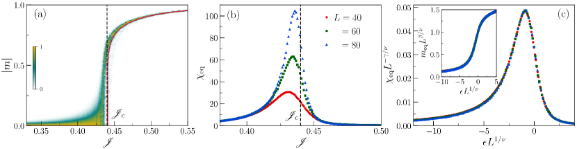
Figure 1: Equilibrium (para-to-ferromagnetic) phase transition of the model, obtained from Monte-Carlo simulations with a minimum of $10^{6}$ independent initial configurations (see text). (a) Magnetization as a function of $\mathscr{J}$ for $L=200$. The solid line shows the exact result in Eq. (7) for $m_{\text{eq}}$, valid as $L\to\infty$. The dashed line marks the critical point, $\mathscr{J}_{c}$ given in Eq. (3). (b) Magnetic susceptibility, $\chi_{\text{eq}}$, as a function of $\mathscr{J}$ for different system sizes. (c) Collapse of the susceptibility (main panel) and magnetization (inset) onto the scaling functions $Y_{\chi_{\text{eq}}}$ and $Y_{m_{\text{eq}}}$, respectively (see text).

Before discussing the finite-time dynamical phase transition in more detail, we review the equilibrium phase transition of the NNIM. For the Monte-Carlo simulations of the model at equilibrium, we employ the Wolff algorithm [33], a non-dynamical algorithm that ensures fast convergence to the equilibrium state, even in the vicinity of the critical point.

An equilibrium phase transition is characterized by a qualitative change of the equilibrium state of a system in response to a quasistatic change of the external parameters [3, 4]. In particular, when $\mathscr{J}$ is increased above $\mathscr{J}_{c}$, the NNIM transitions from a disordered paramagnetic phase to an ordered ferromagnetic phase. The order parameter for this transition is the magnetization $m$ per spin, defined as

$$m=L^{-d}\sum_{i=1}^{N}S_{i}\,.$$ (5)

The spontaneous magnetization $m_{\text{eq}}(L)$ at finite system size $L$ is obtained from

$$m_{\text{eq}}(L)=\langle|m|\rangle\,,$$ (6)

where the brackets $\langle\ldots\rangle$ denote an average over an ensemble of equilibrium systems. In the thermodynamic limit, $m_{\text{eq}}(L)$ converges to the exact expression computed by Onsager [29]:

$$m_{\text{eq}}\equiv\lim_{L\to\infty}m_{\text{eq}}(L)=[1-\sinh^{-4}(2\mathscr{J})]^{1/8}\,.$$ (7)

As its role as an order parameter suggests, $m_{\text{eq}}$ is essentially zero in the paramagnetic phase ($\mathscr{J}<\mathscr{J}_{c}$), while $m_{\text{eq}}>0$ in the ferromagnetic phase ($\mathscr{J}>\mathscr{J}_{c}$).

Figure 1(a) shows the spontaneous magnetization as a function of $\mathscr{J}$ for the two-dimensional NNIM. The heat map represents the probability density of $|m|$ at finite system size, normalized to unity for each $\mathscr{J}$. The solid and dashed lines show $m_{\text{eq}}$ in Eq. (7) and $\mathscr{J}_{c}$ in Eq. (3), respectively. We observe that at fixed $\mathscr{J}$ and for large $L$, the spontaneous magnetization $m_{\text{eq}}$ is well approximated by the regions of largest probability density.

The equilibrium phase transition in the NNIM is continuous, meaning that $m_{\text{eq}}$ changes continuously at the critical point. In the vicinity of this point, several thermodynamic quantities diverge in the thermodynamic limit and exhibit the so-called scaling behavior [34]. For example, from Eq. (7), $m_{\text{eq}}$ behaves as

$$m_{\text{eq}}\sim\epsilon^{\beta}\,,\qquad\epsilon=\frac{\mathscr{J}-\mathscr{J}_{c}}{\mathscr{J}}\,,$$ (8)

for $0<\epsilon\ll 1$, i.e., close to the critical point while approaching from below the critical point, with critical exponent $\beta=\frac{1}{8}$ [35].

Furthermore, the magnetic susceptibility $\chi_{\text{eq}}$ [measured in units of $1/(k_{B}T)$] is determined by Gaussian fluctuations of the magnetization around its mean, i.e.,

$$\chi_{\text{eq}}=L^{d}\left(\langle m^{2}\rangle-\langle|m|\rangle^{2}\right)\,.$$ (9)

Close to the critical point, $\chi_{\text{eq}}$ diverges as

$$\chi_{\text{eq}}\sim|\epsilon|^{-\gamma}\,,$$ (10)

where $\gamma=\frac{7}{4}$ is the associated critical exponent [34, 35].

The exponents, $\beta$ and $\gamma$ have universal values across a range of systems, based on their microscopic symmetries, giving rise to a so-called universality class. In the two-dimensional Ising universality class, $\beta=\frac{1}{8}$ and $\gamma=\frac{7}{4}$ as stated above, while in the mean-field universality class, the corresponding values are $\beta=\frac{1}{2}$ and $\gamma=1$ [35].

II.4 Finite-size scaling

The power-law scalings in Eqs. (8) and (10) are properties of the infinite system. By contrast, whenever the NNIM is studied by means of simulations, one needs to resort to finite systems. Operating at finite system size changes the behavior close to the critical point due to so-called finite-size effects.

Figure 1(b) shows a prime example of a finite-size effect that occurs in the magnetic susceptibility $\chi_{\text{eq}}$ of the NNIM at equilibrium: As a function of the inverse coupling temperature $\mathscr{J}$, $\chi_{\text{eq}}$ does not diverge, as it would according to the predicted behavior in Eq. (10), but exhibits a characteristic peak that becomes more and more pronounced as the system size increases. The location of the peak serves as a finite-size estimate of the critical inverse coupling temperature $\mathscr{J}_{c}(L)$ [36].

Although the divergence of $\chi_{\rm eq}$ in Eq. (10) and the limit $\lim_{L\to\infty}\mathscr{J}_{c}(L)=\mathscr{J}_{c}$ are not directly observable in any finite system, analyzing the finite-size scaling [34, 27, 31, 32] of the system allows one to infer the limiting properties from size-dependent measurements.

Fortunately, for large-enough systems at the critical point, finite-size scaling simplifies, because the correlation length, $\xi_{\text{eq}}$, over which spins are correlated is the only relevant length scale [36]. In the thermodynamic limit, $\xi_{\text{eq}}$ diverges at the critical point as,

$$\xi_{\text{eq}}\sim|\epsilon|^{-\nu}\,,$$ (11)

with an associated exponent $\nu$, whose value is $\nu=1$ in the two-dimensional Ising universality class and $\nu=\frac{1}{2}$ for mean-field models [4].

In finite systems, however, the correlation length $\xi_{\text{eq}}$ is bounded, i.e., cut off, by the system size $L$ at the size-dependent critical inverse coupling temperature $\mathscr{J}_{c}(L)$. Incorporating this, Eqs. (LABEL:ER:beta_eq) and (10) read at the critical point,

$$m_{\text{eq}}(L)\sim L^{-\beta/\nu},\qquad\chi_{\text{eq}}(L)\sim L^{\gamma/\nu}\,,$$ (12)

for $0<\epsilon\ll 1$.

Finite-size effects in $m_{\text{eq}}(L)$ and $\chi_{\text{eq}}(L)$ can be summarized by introducing scaling functions $Y_{m_{\text{eq}}}$ and $Y_{\chi_{\text{eq}}}$, respectively. The function $Y_{m_{\text{eq}}}$ reads

$$Y_{m_{\text{eq}}}(y)=m_{\text{eq}}(L)L^{\beta/\nu}\,,$$ (13)

where $y$ is a dimensionless scaling variable given by

$$y=\text{sign}(\epsilon)\left(\frac{L}{\xi_{\text{eq}}}\right)^{1/\nu}=\epsilon L^{1/\nu}\,.$$ (14)

Similarly, the scaling function $Y_{\chi_{\text{eq}}}$ for the magnetic susceptibility is obtained as

$$Y_{\chi_{\text{eq}}}(y)=\chi_{\text{eq}}(L)L^{-\gamma/\nu}\,.$$ (15)

From Eqs. (12) we observe that both scaling functions are constructed to remain finite at the critical point for any $L$.

The use of scaling functions is that, provided the correct values of the critical exponents $\beta$, $\gamma$, and $\nu$ are known, the rescaled finite-size curves of $m_{\text{eq}}(L)L^{\beta/\nu}$ and for $\chi_{\text{eq}}(L)L^{-\gamma/\nu}$ collapse onto $Y_{m_{\text{eq}}}$ and $Y_{\chi_{\text{eq}}}$, respectively, when plotted against the scaling variable $y$.

Figure 1(c) shows the collapse of the finite-size equilibrium data onto $Y_{\chi_{\text{eq}}}$ and $Y_{m_{\text{eq}}}$ (inset), using the known values for the critical exponents of the two-dimensional Ising universality class stated above. The excellent collapse of the data in Fig. 1(c) confirms that the scaling assumption together with the known values of critical exponents are consistent with the equilibrium data.

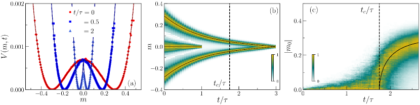
Figure 2: Finite-time dynamical phase transition of the mean-field model for $L=80$, obtained from $10^{6}$ realizations of the relaxation process. (a) Time-dependent rate function $V(m,t)$ as a function of $m$ during a quench from $\mathscr{J}=1.03\mathscr{J}_{c}$ to $\mathscr{J}_{q}=0$. The red line (theory) and red bullets (simulations) show the equilibrium rate function $V_{\text{eq}}$ for $\mathscr{J}=1.03\mathscr{J}_{c}$. The blue lines (theory) and blue symbols (simulations) show $V(m,t)$ at different times, $t/\tau=0.5$ and $2$. (b) Optimal fluctuations before and after the transition, obtained from $5\times 10^{3}$ and $7\times 10^{5}$ conditioned relaxation trajectories, respectively. The solid lines are the optimal fluctuations obtained from theory, the dashed line marks the critical time. (c) Probability distribution of the initial magnetization $|m_{0}|$ at different times, obtained from between $\sim 10^{2}$ (smallest $t/\tau$) to $\sim 10^{5}$ (largest $t/\tau$) conditioned relaxation trajectories. The dashed line denotes the critical time $t_{c}$. The solid lines are obtained from mean-field calculations [17].

II.5 Large-deviation theory

Finite-size fluctuations, both at the critical point and away from it, can be reformulated using large-deviation theory [37]. At large but finite system size, the magnetization $m$ exhibits equilibrium fluctuations. Away from the critical point, the probability density of these fluctuations attains a so-called large-deviation form [37] as $L\to\infty$:

$$P_{\text{eq}}(m)\propto e^{-L^{d}V_{\text{eq}}(m)}\,,$$ (16)

where $V_{\text{eq}}(m)$ denotes the equilibrium rate function, a central object in the theory of large deviations. Here, $V_{\text{eq}}(m)$ measures the exponential rate at which the probability that $m$ takes a given value tends to zero as $L\to\infty$. At the typical (i.e. most likely) event $m=m_{\text{eq}}$, $V_{\text{eq}}(m)$ vanishes, $V_{\text{eq}}(m_{\text{eq}})=0$. The magnetic susceptibility $\chi_{\text{eq}}$, in turn, is given by the inverse of the curvature of $V_{\text{eq}}(m)$ at $m=\pm m_{\text{eq}}$, i.e.,

$$\chi_{\text{eq}}=\frac{1}{V^{\prime\prime}_{\text{eq}}(m_{\text{eq}})}\,.$$ (17)

While $m_{\text{eq}}$ and $\chi_{\text{eq}}$ characterize the mean value and Gaussian fluctuations of $m$, respectively, $V_{\text{eq}}(m)$ also characterizes the leading-order scaling of the probability of large deviations far away from $m=\pm m_{\text{eq}}$.

In the vicinity of the critical point, $\chi_{\text{eq}}$ diverges as the system size tends to infinity, so that the formulation in Eq. (16) breaks down. Instead, critical fluctuations of the magnetization are expressed using the rescaled magnetization $\tilde{m}=mL^{\beta/\nu}$, whose fluctuations are of order unity. As the limit of infinite system size is approached, critical fluctuations are characterized by a universal probability distribution [38, 39]

$$P_{\text{eq}}(\tilde{m},y)\propto e^{-V_{y}(\tilde{m})}\,,$$ (18)

characterized by a scale-invariant rate function $V_{y}(\tilde{m})$, that depends on the scaling variable $y$ defined in Eq. (14), but is independent of the system size.

II.6 Finite-time dynamical phase transition

Having discussed the equilibrium phase transition of the NNIM in some detail, we now proceed to the non-equilibrium scenario. We perform an instantaneous disordering quench of the inverse coupling temperature $\mathscr{J}\to\mathscr{J}_{q}$ from the ordered phase ($\mathscr{J}>\mathscr{J}_{c}$) into the disordered phase ($\mathscr{J}_{q}<\mathscr{J}_{c}$). The quench drives the system far from equilibrium. In the transient that follows, the system relaxes to the new equilibrium state at inverse coupling temperature $\mathscr{J}_{q}$.

During the transient the system evolves with the dynamics described in Sec. II.2. We analyze the evolution of the probability density $P(m,t)$ of the magnetization $m$ as function of time $t$. The large-deviation form (16) then becomes time dependent, i.e.,

$$P(m,t)\propto e^{-L^{d}V(m,t)}\,,$$ (19)

with time-dependent rate function $V(m,t)$. Similar to the equilibrium rate function, $V_{\text{eq}}(m)$, in Eq. (16), $V(m,t)$ measures the exponential rate at which the probability that the magnetization takes the value $m$ at a given time $t$ after the quench tends to zero as $L\to\infty$ .

In the mean-field version of the Ising model, the rate function $V(m,t)$ of the magnetization and of other thermodynamic observables form kink-shaped singular points after sharp finite times [17, 18] in response to the disordering quench. At vanishing magnetic field, the kink in $V(m,t)$ forms at $m=0$ at the critical time [22, 17],

$$t^{MF}_{c}=\frac{\tau}{2(\mathscr{J}_{c}-\mathscr{J}_{q})}\ln\frac{\mathscr{J}-\mathscr{J}_{q}}{\mathscr{J}-\mathscr{J}_{c}}\,.$$ (20)

Figure 2(a) shows the evolution of $V(m,t)$ for the mean-field model. The symbols mark the results of Monte-Carlo simulations, and the solid lines are exact results from mean-field calculations [17]. The initial rate function $V(m,0)=V_{\text{eq}}(m)$ has a characteristic double-well shape, with two characteristic minima that correspond to the typical values $m=\pm m_{\text{eq}}$. As time evolves, the minima of $V(m,t)$ approach the origin and a sharp kink forms at $m=0$. The finite values of the time-dependent rate function $V(0,t)>0$ at $m=0$ imply that the kink is associated with large deviations of the magnetization, generated by rare, extreme relaxation events.

The formation of the kink can be understood as a consequence of competing relaxation dynamics within the system: At $t^{MF}_{c}$, the most likely way the extreme event at $m=0$ is realized, the optimal fluctuation, suddenly switches, resulting in the finite-time dynamical phase transition.

Figure 2(b) shows the optimal fluctuations for $m=0$ in terms of their trajectory densities at different times $t$ before and after $t^{MF}_{c}$. The normalized densities of conditioned relaxation trajectories are shown as a heat-map with yellow regions corresponding to maximum density. Ensembles of conditioned trajectories are obtained by simulating a large number of relaxation trajectories ($\sim 10^{7}$), but keeping only those for which $m$ is within a small window $m=[-\text{d}m,\text{d}m]$ of size $\text{d}m=0.3N^{-1/2}$ at given time $t$. After conditioning, the number of trajectories is substantially reduced to typically between $\sim 10^{3}$ (small $t$) to $\sim 10^{5}$ (larger $t$). The solid lines in Fig. 2(b) are exact results obtained from mean-field computations [17]. The dashed vertical line marks $t^{MF}_{c}$, calculated from Eq. (20).

We observe a marked difference between the typical relaxation to $m=0$ before and after $t^{MF}_{c}$: At times smaller than the critical time, $t<t^{MF}_{c}$, the trajectories that realize $m=0$ are most likely to initiate at $m=0$ at time $t=0$. Although this initial condition is exponentially unlikely, its occurrence is probabilistically favored compared to trajectories that initiate at a more likely initial magnetization (e.g. close to the spontaneous magnetization) but then require many coordinated spin flips to arrive at $m=0$ at time $t$. For times larger than $t_{c}$, by contrast, the situation is reversed: The trajectories that achieve $m=0$ at time $t$ are now most likely to initiate from $m\approx\pm m_{\text{eq}}$, because now a moderate rate of spin flips suffices to reach $m=0$ in the given time window.

To precisely detect and characterize this transition one analyses the probability density of the initial magnetization $m_{0}(t)$, conditioned on relaxing to vanishing magnetization $m=0$ at time $t$. The initial magnetization $m_{0}(t)$ as function of time serves as an order parameter for the finite-time dynamical phase transition, analogous to the magnetization $m$ as function of $\mathscr{J}$ at equilibrium.

Figure 2(c) shows the probability density of the absolute value $|m_{0}|$ of the initial magnetizations of relaxation trajectories that reach $m=0$ at different times $t$ after the disordering quench. The heat map shows the normalized trajectory density, with yellow again corresponding to the highest density. The solid line is from the mean-field calculation [17], valid as $L\to\infty$. The dashed line marks the critical time, Eq. (20).

We note the striking similarity between the behaviors of $|m_{0}|$ as function of $t$ in Fig. 2(c) and of the magnetization $|m|$ as function of $\mathscr{J}$ at equilibrium, shown in Fig. 1(a). Importantly, for the finite-time dynamical phase transition time $t$ takes the role of the control parameter $\mathscr{J}$ at equilibrium [17].

III Results

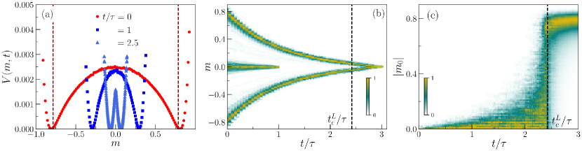
Figure 3: Finite-time dynamical phase transitions in NNIM for $L=60$, obtained from $3\times 10^{6}$ realizations of the relaxation process. (a) Time-dependent rate function $V(m,t)$ as a function of $m$ during a quench from $\mathscr{J}=1.03\mathscr{J}_{c}$ to $\mathscr{J}_{q}=0$. The curve with red symbols show the initial rate function $V_{\text{eq}}(m)$ for $\mathscr{J}=1.03\mathscr{J}_{c}$. The curves with blue symbols show $V(m,t)$ at different times, $t/\tau=1$ and $2.5$. The dashed lines are the spontaneous magnetization at equilibrium for $\mathscr{J}=1.03\mathscr{J}_{c}$. (b) Optimal fluctuations for the NNIM before and after the transition, obtained from $10^{3}$ and $10^{4}$ conditioned relaxation trajectories, respectively. The critical time is marked with the dashed line. (c) Plot of $m_{0}$ during the quench near $m=0$ for NNIM obtained from a range of $\sim 10^{2}$ (smallest $t/\tau$) to $\sim 10^{5}$ (largest $t/\tau$) conditioned trajectories. The dashed line marks the critical time.

The existence of finite-time dynamical phase transitions has been established in both the mean-field model [17, 18] and the NNIM [19]. We now analyze the statistics of the initial magnetization $m_{0}$ (the order parameter) at the critical point, to gain insight into the critical phenomena associated with the finite-time dynamical phase transition in the NNIM.

To this end, we quench a large but finite system from the ordered (ferromagnetic) phase with $\mathscr{J}=1.03\mathscr{J}_{c}>\mathscr{J}_{c}$ into the disordered (paramagnetic) phase where $\mathscr{J}_{q}<\mathscr{J}_{c}$, and evolve it numerically with the spin-flip dynamics discussed in Sec. II.2. To obtain the time-dependent rate function $V(m,t)$ from Eq. (19), we record the evolution of the system and calculate $P(m,t)$ from a large number of (a minimum of $10^{7}$) realizations of the relaxation process.

III.1 Finite-time dynamical phase transition

Figure 3(a) shows the time-dependent rate function $V(m,t)$ of the NNIM, as a function of $m$ at different times after the quench as the colored symbols. The dashed line marks the position of the minima at $\pm m_{\text{eq}}$ in the infinite system size limit, given in Eq. (7). Similar to the rate function of the mean-field model, shown in Fig. 2(a), the rate function of the NNIM forms a kink at $m=0$ during the relaxation. However, due to the finite-size nature of the simulations, the kink is not quite sharp.

More conclusive evidence for the finite-time dynamical phase transitions is obtained by considering the optimal fluctuations that achieve vanishing magnetization, $m=0$, at different times. Figure 3(b) shows the optimal fluctuations that realize vanishing magnetization at short and longer times in terms of their trajectory densities at finite system size. The densities of conditioned relaxation trajectories are shown in terms of a heat map with yellow corresponding to regions of maximum density. The dashed line is the critical time obtained for a method explained in Sec. III.2. We observe a characteristic difference between the optimal fluctuations at short and long times, very similar to the mean-field case [see Fig. 2(b)]: For short times, the optimal fluctuation initiates at an unlikely initial magnetization close to $m=0$ and stays there, while it initiates close to the (most likely) spontaneous magnetization for longer times.

As in the mean-field version of the model, the occurrence of competing relaxation behaviors at short and longer times suggest a finite critical time at which a transition between the two takes place, characterized by the distribution of their initial magnetizations $m_{0}(t)$. Figure 3(c) shows the probability density of $|m_{0}|$ of relaxation trajectories that reach $m=0$ at time $t$. The dashed line marks the critical time $t^{L}_{c}$ obtained numerically using a method explained in Sec. III.2. We observe that $m_{0}$ is essentially zero at short times, but assumes finite values at times longer than $t_{c}^{L}\approx 2.4\tau$. The behavior is analogous to that of $m_{0}(t)$ in the mean-field model shown in Fig. 2(c) and to the statistics of $m$ at equilibrium, see Fig. 1(a).

III.2 Critical time

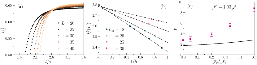
Figure 4: Determination of the critical time from series of finite-size measurements.(a) Dynamical Binder cumulant, $U_{L}^{t}$ (21), as a function of $t/\tau$ for different system sizes. (b) System-size dependent critical time $t_{c}^{L}(L^{\prime})$, obtained from intersections of Binder cumulants for various series of system sizes, see text. The dashed lines show linear fits used to calculate $t_{c}$. (c) Critical time for quenches from $\mathscr{J}=1.03\mathscr{J}_{c}$ to $\mathscr{J}_{q}$. The solid line is from mean-field calculations [17].

Motivated by the striking similarities between the finite-time dynamical phase transition and the equilibrium phase transition [see Figs. 1(a), 2(c), and 3(c)], we apply equilibrium methods to analyze the finite-time dynamical phase transition in vicinity of the critical point $t=t_{c}$.

For equilibrium phase transitions, a common way to obtain critical points is by evaluating the so-called Binder cumulant of the order-parameter distribution [40, 38], defined as $U_{L}^{\rm{eq}}=1-\langle m_{\text{eq}}^{4}\rangle_{L}/(3\langle m_{\text{eq}}^{2}\rangle_{L}^{2})$. In the limit $L\rightarrow\infty$, the Binder cumulant takes the values $0$ and $2/3$ in the paramagnetic phase and the ferromagnetic phase, respectively. At the critical point, $U_{L}^{\rm{eq}}$ is approximately independent of the system size. Therefore, the intersection of different Binder cumulants calculated at different system sizes provides a measure for the location of the critical point from a series of finite-size measurements.

We adopt this method to calculate the critical time $t_{c}$ of the finite-time dynamical phase transition in the NNIM. To this end, we define a dynamical Binder cumulant as

$$U_{L}^{t}=1-\frac{\langle m_{0}^{4}\rangle_{L}}{3\langle m_{0}^{2}\rangle_{L}^{2}}.$$ (21)

Figure 4(a) shows $U_{L}^{t}$ as a function of $t/\tau$. We observe that the Binder cumulants for different system sizes intersect not quite in the same point, but in a small range of $t/\tau$ values. To infer the intersection point of $U_{L}^{t}$ in the thermodynamic limit $L\to\infty$, we compute the intersection of $U_{L}^{t}$ for increasing series of system sizes, thus providing estimates of the system-size dependent critical time, $t_{c}^{L}$.

More precisely, for each system size $L_{m}$, we take a series of larger systems of sizes $L^{\prime}$, differing by a scaling factor $b>1$, i.e., $L^{\prime}=bL_{m}$, so that $L_{m}$ corresponds to the smallest system in each series. For each of these series, we compute the intersections of the Binder cumulants as a function of $b$. Figure 4(b) shows these intersections for different $L_{m}$ with all larger $L^{\prime}>L_{m}$, as function of inverse of the scale factor, $1/b$.

Extrapolation of the data to $1/b\rightarrow 0$ by weighted linear fits (dashed lines) then provides an estimate of the critical time in the thermodynamic limit $L\to\infty$. For $\mathscr{J}_{q}=0$, the average over all such extrapolations gives $t_{c}=2.79\pm 0.36$.

Applying this method at different values of the quenched inverse coupling temperature $\mathscr{J}_{q}$, we obtain $t_{c}$ as function of $\mathscr{J}_{q}$ at fixed $\mathscr{J}=1.03\mathscr{J}_{c}$. Figure 4(c) shows the result of this analysis including error bars for the standard errors. The solid line shows the exact result of the mean-field case given in Eq. (20) [22, 17]. We observe that while the critical time of the mean-field model is consistently smaller, the critical time is a monotonously increasing function of $\mathscr{J}_{q}$ in both cases.

III.3 Generalized susceptibility

After having obtained an estimate of the critical time, we now explore the critical properties of the transition, adopting the finite-size scaling analysis reviewed in Sec. II.4.

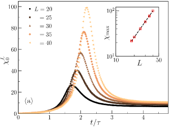
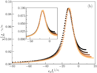
Figure 5: Finite-size scaling of the generalized susceptibility $\chi_{0}^{L}$ (22). (a) $\chi_{0}^{L}$ as a function of $t/\tau$ for different system sizes. Inset: $\chi_{\rm{max}}$ as a function of $L$ on a log-log scale. The dashed line is a power-law fit with exponent $1.90\pm 0.01$ ($=\gamma_{t}/\nu_{t}$). The errors here are within the symbol size. (b) Collapse of $\chi_{0}^{L}$ from different system sizes onto the scaling function $Y_{\chi_{0}^{L}}$ using the parameters $t_{c}=2.79$, $\gamma_{t}/\nu_{t}=1.9$, and $1/\nu_{t}=1$. Inset: Same as in the main frame but with parameters $t_{c}=2.86$, $\gamma_{t}=1.79$, and $\nu_{t}=0.95$, obtained by minimizing $\sigma_{Y_{\chi_{0}}}$ in Eq. (27).

We define the time-dependent, generalized susceptibility $\chi_{0}^{L}$ of the initial magnetization $m_{0}$ at finite system size, the non-equilibrium version of Eq. (9), as

$$\chi_{0}^{L}=L^{d}(\langle m_{0}^{2}\rangle-\langle|m_{0}|\rangle^{2})\,.$$ (22)

In the non-equilibrium case, time plays the role of the inverse coupling temperature in the equilibrium case. We therefore define $\epsilon_{t}\equiv(t-t_{c})/t$ analogously to $\epsilon$ in Eq. (8). As in the case of the equilibrium transition, in the thermodynamic limit, the susceptibility $\chi_{0}$ of the infinite system diverges at the critical point. Analogous to the equilibrium case, we expect the scaling of $\chi_{0}$ as function of $\epsilon_{t}$ to be

$$\chi_{0}\sim|\epsilon_{t}|^{-\gamma_{t}}\,,$$ (23)

where $\gamma_{t}$ denotes the critical exponent associated with the generalized susceptibility. For finite systems, Eq. (23) needs to be modified as $\chi_{0}^{L}(t_{c})\sim L^{\gamma_{t}/\nu_{t}}$, cf. Eq. (12).

The exponent $\nu_{t}$ is the critical exponent associated with the time-dependent correlation length, $\xi_{t}$. Analogous to Eq. (15), we define a dynamical scaling function as,

$$Y_{\chi_{0}}(y_{t})=\chi_{0}^{L}L^{-\gamma_{t}/\nu_{t}},$$ (24)

where

$$y_{t}=\text{sign}(\epsilon_{t})\left(\frac{L}{\xi_{t}}\right)^{1/\nu_{t}}=\epsilon_{t}L^{1/\nu_{t}}\,.$$ (25)

is the time-dependent scaling variable.

Figure 5(a) shows $\chi_{0}^{L}$ for different system sizes. Analogous to $\chi_{\text{eq}}$ in Fig. 1(b), $\chi_{0}^{L}$ shows a pronounced peak whose magnitude becomes larger as the system size increases.

In the perhaps most direct way, $\gamma_{t}/\nu_{t}$ can be estimated from the maximum of the susceptibility, $\chi_{\rm{max}}^{L}$ for different system sizes. $\chi_{\rm{max}}^{L}$ scales with the system size as [36],

$$\chi_{\rm{max}}^{L}\sim L^{\gamma_{t}/\nu_{t}}.$$ (26)

The inset of Fig. 5(a) shows $\chi_{\rm{max}}^{L}$ as a function of $L$ on a log-log scale. The errors are calculated using a bootstrapping method [41]. A power-law fit gives $\gamma_{t}/\nu_{t}=1.90\pm 0.01$ for $\mathscr{J}_{q}=0$. Note that for the linear interpolation to $1/b\to 0$ in our estimate of $t_{c}$ in Sec. III.2, we implicitly assumed $\nu_{t}=1$ [36], consistent with the data given our standard error. Combining these two results, we thus obtain $\gamma_{t}=1.90$, $\nu_{t}=1$, and $t_{c}=2.79$.

As a consistency check, we use these values to collapse the susceptibilities in Fig. 5(a). Figure 5(b) shows a good although not perfect collapse of the data and thus confirms the consistency of the above method.

The slight imperfections in the collapse are probably due to the fact that finite-size effects in the non-equilibrium data arise from multiple sources: the initial configuration, the finite-time conditioning, and the relaxation dynamics. The initial inverse coupling temperature, $\mathscr{J}$, as well as the initial equilibrium rate function $V_{\text{eq}}$ are affected by finite system size because $\mathscr{J}=1.03\mathscr{J}_{c}$ is close to the critical point at equilibrium. However, initiating the system close to $\mathscr{J}_{c}$ is required in order to obtain a sufficiently large ensemble of conditioned relaxation trajectories. In addition, the dynamics is also affected by finite $L$, because first, $L$ needs to be small enough to ensure a sufficient sample size and second, one needs to choose a small (but large enough) window around $m=0$ (of order $\sim N^{-\frac{1}{2}}$ here) for the conditioning on $m=0$ at different $t$. Finite-size effects cumulating from these sources explain why the collapse is less good than in the equilibrium case, cf. Fig. 1(c), which suffers from only one source of finite-size effects.

As a second consistency check, we now compute the parameters $\gamma_{t}$, $\nu_{t}$, and $t_{c}$ by optimizing the data in Fig. 5(a) to achieve the best possible collapse onto the scaling function $Y_{\chi_{0}}$. To this end, we minimize the variance $\sigma_{Y_{\chi_{0}}}$ of the data sets from different system sizes obtained by integrating over a range of scaling variables $y_{t}\in[y^{\rm{min}}_{t},y^{\rm{max}}_{t}]$ near the critical point [32, 42]:

$$\sigma_{x}^{2}=\frac{1}{\Delta y_{t}}\int_{y^{\rm{min}}_{t}}^{y^{\rm{max}}_{t}}\!\!dy_{t}\,\bigg{\{}N_{L}\sum_{L}[Y_{x}(y_{t})]^{2}-\Big{[}\sum_{L}Y_{x}(y_{t})\Big{]}^{2}\bigg{\}}\,,$$ (27)

where $\Delta y_{t}\equiv y^{\rm{max}}_{t}-y^{\rm{min}}_{t}$, $N_{L}$ is the number of system sizes considered, and $Y_{x}(y_{t})$ is the scaling function of either $x=Y_{\chi_{0}}$ or $x=Y_{m_{0}}$ (defined in Sec. III.4).

By minimizing $\sigma_{Y_{\chi_{0}}}$ in this way, we obtain independent estimates for $t_{c}$ and the critical exponents $\gamma_{t}$ and $\nu_{t}$. The inset in Fig. 5(c) shows the collapse for the optimal values, $t_{c}=2.86\pm 0.01$, $\gamma_{t}=1.79\pm 0.01$, and $\nu_{t}=0.95\pm 0.01$.

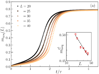
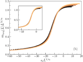
Figure 6: Finite-size scaling of the spontaneous initial magnetization $m_{\text{neq}}(L)$ (28). (a) $m_{\text{neq}}(L)$ as a function of $t/\tau$ for different system sizes. Inset: $m_{\text{neq}}(L)$ at $t_{c}^{L}$, denoted as $m_{\text{neq}}^{t_{c}^{L}}$, as a function of $L$ on log-log scale. The dashed line is a power-law fit with exponent $0.102$ ($=\beta_{t}/\nu_{t}$). (b) Collapse of $m_{\text{neq}}(L)$ onto scaling function $Y_{m_{0}}$ (31) using the parameters $\beta_{t}/\nu_{t}=0.102$, $1/\nu_{t}=1$, and $t_{c}=2.79$. Inset: Same as in the main frame, but with parameters $t_{c}=2.82$, $\beta_{t}=0.093$, and $\nu_{t}=0.92$, obtained from minimizing $\sigma_{Y_{m_{0}}}$, while holding $\beta_{t}/\nu_{t}=0.102$ fixed.

III.4 Initial magnetization

In a similar way, we now extract the critical exponents associated with the initial magnetization, $m_{0}$. In the limit $L\to\infty$, the value of the spontaneous initial magnetization

$$m_{\text{neq}}\equiv\langle|m_{0}|\rangle\,,$$ (28)

vanishes at $t<t_{c}$ but becomes finite for $t>t_{c}$, analogous to $m_{\text{eq}}$ as a function of $\mathscr{J}$ in the equilibrium case. At finite $L$, $m_{\text{neq}}(L)$ is expected to show a similar behavior, although not as sharp. Figure 6(a) shows $m_{\text{neq}}(L)$ for different system sizes. We observe that as $L$ increases $m_{\text{neq}}(L)$ exhibits an increasingly sharp transition to finite values around the critical time $t_{c}\approx 2.8\tau$. In the thermodynamic limit we thus expect the scaling

$$m_{\text{neq}}\sim\epsilon_{t}^{\beta_{t}}\,,$$ (29)

with critical exponent $\beta_{t}$ for the spontaneous initial magnetization, while approaching from above $t_{c}$, analogous to the equilibrium case, cf. Eqs. (12).

For finite $L$, we should instead have

$$m_{\text{neq}}(L)\sim L^{\beta_{t}/\nu_{t}}\,,$$ (30)

at the size-dependent critical time $t=t_{c}^{L}$, obtained with the method in Sec III.2. The inset in Fig. 6(a) shows $m_{\text{neq}}(L)$ at $t_{c}^{L}$, denoted as $m_{\text{neq}}^{t_{c}^{L}}$, as a function of $L$ on a log-log scale. A power-law fit gives the ratio $\beta_{t}/\nu_{t}=\beta_{t}=0.102\pm 0.01$ for $t_{c}=2.79$ and $\mathscr{J}_{q}=0$, where we again implicitly assumed $\nu_{t}=1$ in the interpolation of $t_{c}^{L}$ in Sec. III.2.

To confirm the consistency of these values, we define the analog of Eq. (13), the scaling function $Y_{m_{0}}$, as

$$Y_{m_{0}}(y_{t})=m_{\text{neq}}(L)L^{\beta_{t}/\nu_{t}}\,,$$ (31)

with $y_{t}$ defined in Eq. (25). Figure 6(b) shows how $m_{\text{neq}}(L)$ collapses onto $Y_{m_{0}}$ for the values for $\beta_{t}$, $\nu_{t}$ and $t_{c}$ stated above. The collapse is again satisfactory, although not perfect, showing the consistency of the critical exponents with the data and with the scaling assumption.

To obtain a second, independent estimate, for $\beta_{t}$, $\nu_{t}$ and $t_{c}$, we minimize the variance $\sigma_{Y_{m_{0}}}$ in Eq. (27) to obtain the best possible collapse. In order to make the minimization algorithm converge, we hold the ratio $\beta_{t}/\nu_{t}$ at a fixed value determined by the scaling in Eq. (30). The inset in Fig. 6(b) shows the result of this minimization, yielding the values $t_{c}=2.82\pm 0.02$, $\nu_{t}=0.92\pm 0.02$, $\beta_{t}=0.093\pm 0.006$. We observe that minimizing $\sigma_{Y_{m_{0}}}$ improves the collapse of the data. The values of $t_{c}$ estimated independently from the scaling of $\chi_{0}^{L}$ and $m_{\text{neq}}(L)$ lie within the errors of the critical times estimated in Sec. III.2.

III.5 Critical exponents

Figure 7: Critical exponents, $\beta_{t}$, $\gamma_{t}$, and $\nu_{t}$ for different $\mathscr{J}_{q}$. Dashed horizontal lines correspond to the exponents in the two dimensional Ising universality class. All exponents are determined from two different methods (see text).

Repeating the analysis summarized in Secs. III.3 and III.4 for different quenched inverse coupling temperatures $\mathscr{J}_{q}$, we obtain the critical exponents $\beta_{t}$, $\gamma_{t}$ and $\nu_{t}$ as function of $\mathscr{J}_{q}$. Figure 7 shows the result of this analysis as symbols. The dashed lines show the corresponding exponents from the two dimensional Ising universality class. For each of the critical exponents, we obtain two estimates, given as different symbols. The green squares and yellow triangles for $\nu_{t}$ are obtained from minimizing $\sigma_{x}$ for $\chi_{0}^{L}$ and $m_{0}$, respectively. The symbols for $\gamma_{t}$ are obtained from the scaling of $\chi_{\rm{max}}$ (in black triangles) and minimizing $Y_{\chi_{0}}$ (in blue squares). For $\beta_{t}$ the symbols are obtained from the scaling of $m_{\text{neq}}^{t_{c}^{L}}$ (brown circles) and from minimizing $\sigma_{Y_{m_{0}}}$ (red triangles). We observe that although the critical time $t_{c}$ depends on the initial and final point of the quenching process, see Fig. 4(c), the critical exponents stay approximately constant, and are consistent with the values of the two-dimensional Ising universality class.

In other words, just as for the mean-field model [17], the values of the dynamical critical exponents $\beta_{t}$, $\gamma_{t}$, and $\nu_{t}$ of the disordering quench appear to be identical to the exponents $\beta$, $\gamma$ and $\nu$ of the corresponding equilibrium phase transition, across which the system is initially quenched.

It is worth noting that this also implies that $\beta_{t}$, $\gamma_{t}$, and $\nu_{t}$ obey a so-called hyper-scaling relation [34]

$$\nu_{t}d=2\beta_{t}+\gamma_{t}\,,$$ (32)

connecting all critical exponents. Here, $d=2$ denotes the spatial dimension. The validity of Eq. (32) is consistent with the initial assumption that the correlation length $\xi_{t}$ is the only relevant length scale in the infinite system close to the critical point [36].

As an example for the validity of the hyper-scaling in Eq. (32), consider the quench from $\mathscr{J}=1.03\mathscr{J}_{c}$ to $\mathscr{J}_{q}=0$. The value for $\nu_{t}d-(2\beta_{t}+\gamma_{t})$ comes out to be $-0.07\pm 0.1$, which is consistent with $0$.

IV Conclusions

We have studied critical phenomena associated with the finite-time dynamical phase transition of the nearest-neighbor Ising model on a two-dimensional square-lattice by means of Monte Carlo simulations. The transition manifests as a finite-time switch in the mostly likely relaxation dynamics, the optimal fluctuation, after a disordering quench from the ferro-magnetic phase into the paramagnetic phase [17, 18, 19]. The initial magnetization $m_{0}(t)$ associated with the optimal fluctuation of the relaxation dynamics that achieves $m=0$ at given time $t$ serves as an order parameter for the transition, similar to the magnetization at equilibrium.

Using a finite-size scaling analysis, we extracted both the critical time $t_{c}$ at which the transition occurs, as well as the associated critical exponents from the statistics of $m_{0}$. Near the critical point, the fluctuations of $m_{0}$, measured by the generalized susceptibility $\chi_{0}$, diverge and exhibit characteristics of a continuous equilibrium phase transition. We thus explored the critical fluctuations of $m_{0}$ using the scaling functions $Y_{m_{0}}$ and $Y_{\chi_{0}}$ associated with $m_{0}$ and $\chi_{0}$, respectively. From this analysis, we estimated the dynamical critical exponents, $\beta_{t}$, $\gamma_{t}$ and $\nu_{t}$ corresponding to the initial magnetization $m_{0}$, the generalized susceptibility $\chi_{0}$ and the correlation length $\xi_{t}$ of $m_{0}$, respectively. The obtained values of these exponents are consistent with the values of the corresponding exponents in the equilibrium counter-part of the model, and they obey a hyper-scaling relation, Eq. (32).

We conclude that the finite-time dynamical phase transition in the nearest-neighbor Ising model belongs to the same universality class as the corresponding equilibrium model, consistent with the results from the mean-field model [17], where similar conclusions were drawn.

The dependence of the critical time $t_{c}$ on the final (and initial) inverse coupling temperatures of the quench, $\mathscr{J}$ and $\mathscr{J}_{q}$, respectively, suggests that correlations between spins in the initial and final states of the transition play an important role. In the future, we intend to analyze the spatial structure of the Ising model during the relaxation process achieving $m=0$ at given time $t$, to obtain a clearer understanding of, e.g., the monotonous dependence $t_{c}$ on the external parameters.

Furthermore, it would also be interesting to investigate the finite-time dynamical phase transition in higher dimensions $d>2$. This would clarify whether or not the dynamical critical exponents agree with the equilibrium one also in this case. Crucially, at equilibrium the nearest-neighbor Ising model becomes mean-field like for $d\geq 4$, and it is a fascinating open question if this behavior is paralleled in the non-equilibrium transition. The use of phenomenological theories such as Ginzburg-Landau theory [43, 44] could perhaps be useful to elucidate these questions.

References

- Haken and Haken [2004] H. Haken and H. Haken, An introduction: nonequilibrium phase transitions and self-organization in physics, chemistry and biology, Synergetics: Introduction and Advanced Topics , 1 (2004).
- Cross and Hohenberg [1993] M. C. Cross and P. C. Hohenberg, Pattern formation outside of equilibrium, Rev. Mod. Phys. 65, 851 (1993).
- Landau and Lifshitz [2012] L. D. Landau and E. M. Lifshitz, Course of theoretical physics Volume 5: Statistical Physics Part 1 (Elsevier, 2012).
- Goldenfeld [2018] N. Goldenfeld, Lectures on phase transitions and the renormalization group (CRC Press, 2018).
- Marconi et al. [2008] U. M. B. Marconi, A. Puglisi, L. Rondoni, and A. Vulpiani, Fluctuation–dissipation: response theory in statistical physics, Phys. Rep. 461, 111 (2008).
- Baiesi and Maes [2013] M. Baiesi and C. Maes, An update on the nonequilibrium linear response, New J. Phys. 15, 013004 (2013).
- Bray [2002a] A. J. Bray, Theory of phase-ordering kinetics, Adv. Phys. 51, 481 (2002a).
- Mpemba and Osborne [1969] E. B. Mpemba and D. G. Osborne, Cool?, Phys. Educ. 4, 172 (1969).
- Lu and Raz [2017] Z. Lu and O. Raz, Nonequilibrium thermodynamics of the markovian mpemba effect and its inverse, Proceedings of the National Academy of Sciences 114, 5083 (2017).
- Kovacs et al. [1963] A. Kovacs, R. A. Stratton, and J. D. Ferry, Dynamic mechanical properties of polyvinyl acetate in shear in the glass transition temperature range, The Journal of Physical Chemistry 67, 152 (1963).
- Kovacs et al. [1979] A. J. Kovacs, J. J. Aklonis, J. M. Hutchinson, and A. R. Ramos, Isobaric volume and enthalpy recovery of glasses. II. A transparent multiparameter theory, J. Polym. Sci. Polym. Phys. Ed. 17, 1097 (1979).
- Bertin et al. [2003] E. Bertin, J. Bouchaud, J. Drouffe, and C. Godreche, The kovacs effect in model glasses, Journal of physics A: mathematical and general 36, 10701 (2003).
- Lapolla and Godec [2020] A. Lapolla and A. Godec, Faster uphill relaxation in thermodynamically equidistant temperature quenches, Phys. Rev. Lett. 125, 110602 (2020).
- Meibohm et al. [2021] J. Meibohm, D. Forastiere, T. Adeleke-Larodo, and K. Proesmans, Relaxation-speed crossover in anharmonic potentials, Phys. Rev. E 104, L032105 (2021).
- Ibáñez et al. [2024] M. Ibáñez, C. Dieball, A. Lasanta, A. Godec, and R. A. Rica, Heating and cooling are fundamentally asymmetric and evolve along distinct pathways, Nat. Phys. 20, 135 (2024).
- Holtzman and Raz [2022] R. Holtzman and O. Raz, Landau theory for the Mpemba effect through phase transitions, Commun. Phys. 5, 280 (2022).
- Meibohm and Esposito [2022] J. Meibohm and M. Esposito, Finite-time dynamical phase transition in nonequilibrium relaxation, Phys. Rev. Lett. 128, 110603 (2022).
- Meibohm and Esposito [2023] J. Meibohm and M. Esposito, Landau theory for finite-time dynamical phase transitions, New J. Phys. 25, 023034 (2023).
- Blom and Godec [2022] K. Blom and A. Godec, Global speed limit for finite-time dynamical phase transition in nonequilibrium relaxation, arXiv preprint arXiv:2209.14287 https://doi.org/10.48550/arXiv.2209.14287 (2022).
- Van Enter et al. [2002] A. Van Enter, R. Fernández, F. Den Hollander, and F. Redig, Possible loss and recovery of Gibbsianness during the stochastic evolution of Gibbs measures, Commun. Math. Phys. 226, 101 (2002).
- Külske and Le Ny [2007] C. Külske and A. Le Ny, Spin-flip dynamics of the Curie-Weiss model: Loss of Gibbsianness with possibly broken symmetry, Commun. Math. Phys. 271, 431 (2007).
- Ermolaev and Külske [2010] V. Ermolaev and C. Külske, Low-temperature dynamics of the Curie-Weiss model: Periodic orbits, multiple histories, and loss of Gibbsianness, J. Stat. Phys. 141, 727 (2010).
- Redig and Wang [2012] F. Redig and F. Wang, Gibbs-non-Gibbs transitions via large deviations: computable examples, J. Stat. Phys. 147, 1094 (2012).
- Täuber [2014] U. C. Täuber, Critical dynamics: a field theory approach to equilibrium and non-equilibrium scaling behavior (Cambridge University Press, 2014).
- Baglietto and Albano [2008] G. Baglietto and E. V. Albano, Finite-size scaling analysis and dynamic study of the critical behavior of a model for the collective displacement of self-driven individuals, Phys. Rev. E 78, 021125 (2008).
- Wood et al. [2006] K. Wood, C. Van den Broeck, R. Kawai, and K. Lindenberg, Universality of synchrony: critical behavior in a discrete model of stochastic phase-coupled oscillators, Phys. Rev. Lett. 96, 145701 (2006).
- Fisher and Barber [1972] M. E. Fisher and M. N. Barber, Scaling theory for finite-size effects in the critical region, Phys. Rev. Lett. 28, 1516 (1972).
- Griffiths et al. [1966] R. B. Griffiths, C.-Y. Weng, and J. S. Langer, Relaxation times for metastable states in the mean-field model of a ferromagnet, Phys. Rev. 149, 301 (1966).
- Onsager [1944] L. Onsager, Crystal statistics. I. A two-dimensional model with an order-disorder transition, Phys. Rev. 65, 117 (1944).
- Glauber [1963] R. J. Glauber, Time-dependent statistics of the Ising model, J. Math. Phys. 4, 294 (1963).
- Landau and Binder [2021] D. P. Landau and K. Binder, A guide to Monte Carlo simulations in statistical physics (Cambridge university press, 2021).
- Newman and Barkema [1999] M. E. Newman and G. T. Barkema, Monte Carlo methods in statistical physics (Clarendon Press, 1999).
- Wolff [1989] U. Wolff, Collective Monte Carlo updating for spin systems, Phys. Rev. Lett. 62, 361 (1989).
- Fisher [1967] M. E. Fisher, The theory of equilibrium critical phenomena, Rep. Prog. Phys. 30, 615 (1967).
- Stanley [1971] H. E. Stanley, Phase transitions and critical phenomena, Vol. 7 (Clarendon Press, Oxford, 1971).
- Binder [1990] K. Binder, in Finite size scaling and numerical simulation of statistical systems, edited by V. Privman (World Scientific, 1990).
- Touchette [2009] H. Touchette, The large deviation approach to statistical mechanics, Phys. Rep. 478, 1 (2009).
- Binder [1981a] K. Binder, Critical properties from Monte Carlo coarse graining and renormalization, Phys. Rev. Lett. 47, 693 (1981a).
- Balog et al. [2022] I. Balog, A. Rançon, and B. Delamotte, Critical probability distributions of the order parameter from the functional renormalization group, Phys. Rev. Lett. 129, 210602 (2022).
- Binder [1981b] K. Binder, Finite size scaling analysis of Ising model block distribution functions, Z. Physik B Cond. Mat. 43, 119 (1981b).
- Efron [1992] B. Efron, Bootstrap methods: another look at the jackknife, in Breakthroughs in statistics: Methodology and distribution (Springer, 1992) pp. 569–593.
- Newman and Barkema [1996] M. E. Newman and G. T. Barkema, Monte Carlo study of the random-field Ising model, Phys. Rev. E 53, 393 (1996).
- Bray [2002b] A. J. Bray, Theory of phase-ordering kinetics, Adv. Phys. 51, 481 (2002b).
- Hohenberg and Halperin [1977] P. C. Hohenberg and B. I. Halperin, Theory of dynamic critical phenomena, Rev. Mod. Phys. 49, 435 (1977).
- Varrette et al. [2022] S. Varrette, H. Cartiaux, S. Peter, E. Kieffer, T. Valette, and A. Olloh, Management of an Academic HPC & Research Computing Facility: The ULHPC Experience 2.0, in Proc. of the 6th ACM High Performance Computing and Cluster Technologies Conf. (HPCCT 2022) (Association for Computing Machinery (ACM), Fuzhou, China, 2022).