Online Concurrent Multi-Robot Coverage Path Planning

Abstract

Recently, centralized receding horizon online multi-robot coverage path planning algorithms have shown remarkable scalability in thoroughly exploring large, complex, unknown workspaces with many robots. In a horizon, the path planning and the path execution interleave, meaning when the path planning occurs for robots with no paths, the robots with outstanding paths do not execute, and subsequently, when the robots with new or outstanding paths execute to reach respective goals, path planning does not occur for those robots yet to get new paths, leading to wastage of both the robotic and the computation resources. As a remedy, we propose a centralized algorithm that is not horizon-based. It plans paths at any time for a subset of robots with no paths, i.e., who have reached their previously assigned goals, while the rest execute their outstanding paths, thereby enabling concurrent planning and execution. We formally prove that the proposed algorithm ensures complete coverage of an unknown workspace and analyze its time complexity. To demonstrate scalability, we evaluate our algorithm to cover eight large $2$D grid benchmark workspaces with up to $512$ aerial and ground robots, respectively. A comparison with a state-of-the-art horizon-based algorithm shows its superiority in completing the coverage with up to $1.6\times$ speedup. For validation, we perform ROS + Gazebo simulations in six $2$D grid benchmark workspaces with $10$ Quadcopters and TurtleBots, respectively. We also successfully conducted one outdoor experiment with three quadcopters and one indoor with two TurtleBots.

I Introduction

Coverage Path Planning (CPP) determines conflict-free paths for a group of mobile robots so they can visit obstacle-free sections of a particular workspace to perform a given task. It has many indoor (e.g., cleaning[1] and industrial inspection[2]) and outdoor (e.g., precision agriculture[3], surveying[4], and disaster management[5]) applications. A CPP algorithm is also known as a Coverage Planner (CP), and its primary objective is to ensure complete coverage, meaning the robots visit the entire obstacle-free section of the workspace. While a single robot (e.g., [6, 7, 8]) can cover a small workspace, it may take too long to cover a large workspace. Multiple robots (e.g., [9, 10, 11, 12, 13, 14]) can cover a large workspace faster if the CP distributes the workload fairly among the robots. However, designing a CP that can supervise many robots efficiently is challenging.

We call a CP offline if the workspace is known, i.e., the CP knows the obstacle placements beforehand (e.g., [15, 16, 17]). So, it finds the robots’ paths all at once. In contrast, we call a CP online if the workspace is unknown, i.e., the CP has no prior knowledge about the obstacle placements (e.g., [18, 19, 20, 21]). So, it runs numerous iterations to cover the workspace gradually. The robots send sensed data, acquired through attached sensors, about the explored workspace sections to the CP in each iteration, and the CP finds subpaths that the robots follow to visit obstacle-free sections not visited so far and explore more of the workspace.

We classify a CP as centralized (e.g., [18, 6, 7, 22, 8]), which runs in a server and solely obtains all the robots’ paths, or distributed (e.g., [19, 23]), which runs in each robot as a local instance. These local instances collaborate among themselves to obtain individual paths. Recently, for large unknown workspaces, centralized horizon-based (e.g., [24, 22]) algorithm GAMRCPP [25] has shown its scalability in finding shorter length paths for many robots (up to 128) by exploiting the global state space, thereby completing the coverage faster than distributed algorithm $\mathtt{BoB}$ [23].

Centralized online multi-robot horizon-based CPs, like [22, 25, 26], in each horizon, attempts to plan paths for either all the robots (e.g., [22] and [25]) or a subset of robots (e.g., [26]), called the participants, who have entirely traversed their last planned paths. Therefore, the participants do not have any remaining paths to follow, demanding new paths from the CP. The rest (if any), called the non-participants, are yet to finish following their last planned paths, so they have remaining paths left to follow. Due to the interleaving of path planning (by the CP) and subsequently path following (by the robots) in each horizon of these CPs, they suffer from the wastage of robotic resources in two ways. When the CP replans the participants, the non-participants wait until the planning ends. Another, while the active participants (the participants for whom the CP has found the paths) and the non-participants of the current horizon follow their paths, the inactive participants wait for reconsideration by the CP in the next horizon till the path following is over. The latter is also a waste of computation resources.

In this paper, we design a centralized online multi-robot non-horizon-based CP, where planning and execution of paths happen in parallel. It makes the CP design extremely challenging because while planning the participants’ conflict-free paths on demand, it must accurately infer the remaining paths of the non-participants. The proposed CP timestamps the active participants’ paths with a discrete global clock value, meaning the active participants must follow respective paths from that time point. Hence, path execution happens in sync with the global clock. However, path planning happens anytime if there is a participant. Thus, the CP enables overlapping path planning with path execution, significantly reducing the time required to complete the coverage with hundreds of robots.

We formally prove that our CP ensures complete coverage of an unknown workspace and then analyze its time complexity. We evaluate our CP on eight large $2$D grid benchmark workspaces with up to $512$ aerial and ground robots, respectively. The results justify its scalability by outperforming the state-of-the-art OnDemCPP, which previously outperformed GAMRCPP, completing the coverage of large unknown workspaces faster with hundreds of robots. We validate the CP through ROS + Gazebo simulations on six $2$D grid benchmark workspaces with $10$ aerial and ground robots, respectively. Moreover, we perform two experiments with real robots — One outdoor experiment with three quadcopters and another indoor with two TurtleBots.

II Problem

II-A Preliminaries

Let $\mathbb{R}$ and $\mathbb{N}$ denote the set of real numbers and natural numbers, respectively, and $\mathbb{N}_{0}$ denotes the set $\mathbb{N}\cup\{0\}$. Also, for $m\in\mathbb{N}$, $[m]=\{n\in\mathbb{N}\,|\,n\leq m\}$ and $[m]_{0}=[m]\cup\{0\}$. The size of the countable set $\mathcal{S}$ is denoted by $|\mathcal{S}|\in\mathbb{N}_{0}$. Furthermore, we denote the Boolean values $\{0,1\}$ by $\mathbb{B}$.

II-A1 Workspace

We consider an unknown $2$D grid workspace $W$ of size $X\times Y$, where $X,Y\in\mathbb{N}$ are its size along the $x$ and the $y$ axes, respectively. So, $W$ consists of square-shaped equal-sized non-overlapping cells $\{(x,y)\ |\ x\in[X]\land y\in[Y]\}$. Some of these cells are obstacle-free (denoted by $W_{free}$), hence traversable. The rest are fully occupied with static obstacles (denoted by $W_{obs}$), hence not traversable. Note that $W_{free}$ and $W_{obs}$ are unknown initially, and $W=W_{free}\cup W_{obs}$ and $W_{free}\cap W_{obs}=\emptyset$. We assume that $W_{free}$ is strongly connected.

II-A2 Robots and their States

We employ a team of $R\in\mathbb{N}$ homogeneous failure-free robots, where each robot fits entirely within a cell. We denote the $i(\in[R])$-th robot by $r^{i}$ and assume that the robots are location-aware. So, we denote the state of $r^{i}$ at the $j(\in\mathbb{N}_{0})$-th discrete time step by $s^{i}_{0}$, which is a tuple of its location and possibly orientation in $W$. We define a function $\mathcal{L}$, which takes a state $s$ as input and returns the corresponding location $\mathcal{L}(s)\in W$ as a tuple. Initially, the robots get randomly deployed at different cells in $W_{free}$, comprising the set of start states $S=\{s^{i}_{0}\ |\ i\in[R]\land\mathcal{L}(s^{i}_{0})\in W_{free}\land\forall j(\neq i)\in[R]\ \mathcal{L}(s^{i}_{0})\neq\mathcal{L}(s^{j}_{0})\}$. We also assume that each $r^{i}$ is fitted with four rangefinders on all four sides to detect obstacles in those neighboring cells.

II-A3 Motions and generated Paths

The robots have a set of motion primitives $M$ to change their states in each time step. It contains a unique motion primitive $\mathtt{Halt(H)}$ to keep a state unchanged in the next step. Each motion primitive $\mu\in M$ is associated with some cost $\mathtt{cost(\mu)}\in\mathbb{R}$ (e.g., distance traversed, energy consumed, etc.), but we assume that they all take the same $\tau\in\mathbb{R}$ amount of time for execution.

Initially, the path $\pi^{i}$ of robot $r^{i}$ contains its start state $s^{i}_{0}$. So, the length of $\pi^{i}$, denoted by $|\pi^{i}|$, is $0$. When a sequence of motion primitives $(\mu_{j}\in M)_{j\in[\Lambda]}$ of length $\Lambda\in\mathbb{N}$ gets applied on $s^{i}_{0}$, it results in a $\Lambda$-length path $\pi^{i}$, i.e., $|\pi^{i}|=\Lambda$. Therefore, $\pi^{i}$ contains a sequence of states of $r^{i}$ s.t. $s^{i}_{j-1}\xrightarrow{\mu_{j}}s^{i}_{j},\forall j\in[\Lambda]$. Note that we can make all the path lengths equal to $\Lambda$ by suitably applying $\mathtt{H}$ motions at their ends. The resultant set of paths is $\Pi=\{\pi^{i}\ |\ i\in[R]\land|\pi^{i}|=\Lambda\}$, where each $\pi^{i}$ satisfies the following three conditions:

1. $\forall j\in[\Lambda]_{0}\ \mathcal{L}(s^{i}_{j})\in W_{free}$,                 [Avoid obstacles]

2. $\forall j\in[\Lambda]_{0}\ \forall k\in[R]\setminus\{i\}\\ \mathcal{L}(s^{i}_{j})\neq\mathcal{L}(s^{k}_{j})$,                 [Avert same cell collisions]

3. $\forall j\in[\Lambda]\ \forall k\in[R]\setminus\{i\}\\ \lnot((\mathcal{L}(s^{i}_{j-1})=\mathcal{L}(s^{k}_{j}))\wedge(\mathcal{L}(s^{i}_{j})=\mathcal{L}(s^{k}_{j-1})))$.
   BLANK                             [Avert head-on collisions]

Further, we define the cost of a path $\pi^{i}$, denoted by $\mathtt{cost}(\pi^{i})\in\mathbb{R}$, as the sum of its motions’ costs, i.e., $\mathtt{cost}(\pi^{i})=\sum_{j\in[\Lambda]}\mathtt{cost}(\mu_{j})$.

Example 1

To illustrate using an example, we consider TurtleBot [27], which rotates around its axis and drives forward. So, the state of a TurtleBot is $s^{i}_{j}=(x,y,\theta)$, where $(x,y)\in W$ is its location and $\theta\in\{\mathtt{East(E)},\mathtt{West(W)},\mathtt{North(N)},\mathtt{South(S)}\}$ is its orientation in $W$. The motions of a TurtleBot are $M=\{\mathtt{Halt(H)},\mathtt{TurnRight(TR)},\mathtt{TurnLeft(TL)},\mathtt{MoveNext(MN)}\}$, where $\mathtt{TR}$ and $\mathtt{TL}$ rotate a TurtleBot $90^{\circ}$ clockwise and counterclockwise, respectively, and $\mathtt{MN}$ moves it to the next cell pointed by its orientation $\theta$.

II-B Problem Definition

Problem 1 (Complete Coverage Path Planning Problem)

Formally, it is defined as a problem $\mathcal{P}_{CPP}$, which takes an unknown workspace $W$, a team of $R$ robots with their start states $S$ and motions $M$, and generates their obstacle avoiding and inter-robot collision averting paths $\Pi$ to ensure each obstacle-free cell gets visited by at least one robot:

$\Pi=\mathcal{P}_{CPP}(W,R,S,M)$ s.t. $\cup_{i\in[R]}\cup_{j\in[\Lambda]_{0}}\mathcal{L}(s^{i}_{j})=W_{free}$.

III Concurrent CPP Framework

This section presents the proposed centralized concurrent CPP framework that makes a team of mobile robots cover an unknown workspace completely, whose size and boundary are only known to the CP and the robots.

To ensure space-time consistency of the robots’ paths, the CP runs a global discrete clock $CLK\in\mathbb{N}_{0}$ that increments after each $\tau\ $\mathrm{s}$$ (the motion primitive execution time) and the clocks at the robots are in sync with it using a clock synchronization protocol [28]. Each robot has its initial perception of the workspace, called local view, as the fitted rangefinders are range-limited. Initially, all the robots participate in planning, so they send their local views to the CP through request messages for paths. When the CP receives any request, it immediately updates the global view of the workspace using the local view. After receiving the intended number of requests, the CP uses the global view to generate paths, possibly of different lengths, for the participants. The participants for which the CP has found paths are said to be active while the rest are said to be inactive. The CP, while generating the paths, timestamps them with a particular $CLK$ value, signifying the active participants must follow their respective path from that specified $CLK$ value. Now, the CP simultaneously sends paths to those active participants through response messages. The robots that receive responses follow their respective paths from the timestamped $CLK$ and update their local views accordingly. As a robot finishes following its path, it sends its updated local view to the CP. Upon receiving, first, the CP updates the global view, and then it begins the next planning round if some preset conditions are satisfied. At the end of any current planning round, the CP checks the preset conditions to begin the next planning round for inactive participants, new participants, or both. Thus, the path planning is on-demand, where the CP replans for the participants who have entirely traversed their previously planned paths but without modifying the non-participants’ existing paths. And, the path following is synchronous w.r.t. $CLK$. Moreover, path planning for the participants can happen in parallel with the path execution by the non-participants, hence concurrent CPP. Note that the CP allows only one instance of planning round at a time, which can begin or end at any time.

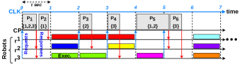
Figure 1: Overview of concurrent CPP

Example 2

In Figure 1, we show a schematic diagram of the overall concurrent CPP framework for three robots in an arbitrary workspace. In the initial planning round P₁, the CP finds paths timestamped with $1$ for participants $r^{2}$ and $r^{3}$ only. So, it begins P₂ for the inactive participant $r^{1}$ of P₁, whose path gets timestamped with $1$ as well. When the CP replans $r^{2}$ in P₃, non-participants $r^{1}$ and $r^{3}$ follow their existing paths in parallel. The new path of $r^{2}$ (observe the new color) gets timestamped with $3$. Similarly, it replans $r^{3}$ in P₄, whose path gets timestamped with $4$. However, in P₅, by the time it ends replanning $r^{1}$ and $r^{2}$, whose paths get timestamped with $6$, it receives a new request from $r^{3}$. So, it replans for $r^{3}$ in P₆, whose path gets timestamped with $6$ also.

III-A Data structures at CP

Let $I_{par}\subseteq[R]$ be the set of IDs of the robots participating in the coming planning round, and $S$ be the set of their corresponding states. Also, let $\eta\in[R]_{0}$ be the number of participants needed to begin the coming planning round, which the CP sets dynamically after each planning round to replan for inactive participants or new participants. By $T_{stop}$, we denote an array of size $R$, where $T_{stop}[i]\in\mathbb{N}_{0}$ denotes the $CLK$ value when $r^{i}$ finishes following its latest path.

III-B Overall Concurrent Coverage Path Planning

1

2

3$W^{i}\leftarrow\mathtt{init\_localview}(s^{i}_{0},X,Y)$

$\mathtt{M_{req}[id,state,view]}\leftarrow[i,s^{i}_{0},W^{i}]$

  // Create $\mathtt{M_{req}}$

4

5while true do

6      $\mathtt{send\_localview(M_{req})}$

7      $\langle\sigma^{i},T_{start}\rangle\leftarrow\mathtt{receive\_path(M_{res})}$

8      $W^{i}\leftarrow\mathtt{follow\_path}(\sigma^{i},T_{start})$

      $\mathtt{M_{req}[state,view]}\leftarrow[s^{i}_{|\sigma^{i}|},W^{i}]$

       // Update $\mathtt{M_{req}}$

9     

Algorithm 1 $\mathtt{Robot}(i,s^{i}_{0},X,Y)$

In this section, we explain the overall concurrent CPP in detail with the help of Algorithms 1 and 2. First, we explain Algorithm 1, which runs at each robot $r^{i}$. At the beginning, $r^{i}$ initializes its local view $W^{i}=\langle W^{i}_{u},W^{i}_{o},W^{i}_{g},W^{i}_{c}\rangle$ (line 1), where $W^{i}_{u}$, $W^{i}_{o}$, $W^{i}_{g}$, and $W^{i}_{c}$ are the set of unexplored cells, obstacles (explored cells that are obstacle-occupied), goals (explored cells that are obstacle-free and yet to get visited), and covered (explored cells that are obstacle-free and have already been visited) cells, respectively. Next, it creates a request message $\mathtt{M_{req}}$, containing its $\mathtt{id}\ i$, current $\mathtt{state}\ s^{i}_{0}$, and local $\mathtt{view}\ W^{i}$ (line 2). Then, it sends the $\mathtt{M_{req}}$ to the CP (line 4) and waits for the response message $\mathtt{M_{res}}$ to arrive (line 5). Upon arrival, it extracts its path $\sigma^{i}$ and associated timestamp $T_{start}\in\mathbb{N}$ from the $\mathtt{M_{res}}$, and starts following $\sigma^{i}$ from $T_{start}$ (line 6). While following, it uses its rangefinders to explore previously unexplored workspace cells and updates $W^{i}$ accordingly. Finally, it reaches its goal $\mathcal{L}(s^{i}_{|\sigma^{i}|})$ corresponding to the state $s^{i}_{|\sigma^{i}|}$ when $CLK$ becomes $T_{start}+|\sigma^{i}|$. So, it updates the $\mathtt{M_{req}}$ with $s^{i}_{|\sigma^{i}|}$ and $W^{i}$ (line 7) and sends it to the CP in a while loop (lines 3-7).

1

2

3

$I_{par}\leftarrow\emptyset,S\leftarrow\emptyset,W\leftarrow\emptyset$

  // Init.

$\eta\leftarrow R$

  // Intended number of participants

4 $\Pi\leftarrow\{\pi^{i}\ |\ i\in[R]\}$ where $\pi^{i}\leftarrow s^{i}_{0}$

5 $T_{stop}[i]\leftarrow 0,\forall i\in[R]$

6 Service receive_localview($\mathtt{M_{req}}$):

7      $I_{par}\leftarrow I_{par}\cup\{\mathtt{M_{req}.id}\}$

8      $S\leftarrow S\cup\{\mathtt{M_{req}.state}\}$

9      $W\leftarrow\mathtt{update\_globalview(M_{req}.view)}$

10      check_CPP_criteria()

11     

12      Function check_CPP_criteria():

13           if $|I_{par}|=\eta$ then

14                $\widetilde{W_{g}}\leftarrow\mathtt{get\_reserved\_goals}(\overline{I_{par}},\Pi)$

15                if $(W_{g}\setminus\widetilde{W_{g}})\neq\emptyset$ then // Start

                     $W^{*}\leftarrow W$

                      // Take snapshot

16                     $I^{*}_{par}\leftarrow I_{par}$

17                     $S^{*}\leftarrow S$

                     $I_{par}\leftarrow\emptyset,S\leftarrow\emptyset$

                      // Reinit.

18                     $\eta\leftarrow 0$

19                     $\mathtt{THD}$.ConCPP_Round($W^{*},\widetilde{W_{g}},I^{*}_{par},S^{*}$)

20                    

21                     else if $|I_{par}|=R$ then // Stop (Coverage Complete)

22                          exit ()

23                         

24                          else  // Skip

25                               increment_eta ($\overline{I_{par}}$)

26                              

27                              

28                              

29                               Function increment_eta($I$):

30                                    $T_{min}\leftarrow\min\{T_{stop}[i]\ |\ i\in I\land\ T_{stop}[i]>CLK\}$

31                                    for $i\in I$ do

32                                         if $T_{stop}[i]=T_{min}$ then

                                              $\eta\leftarrow\eta+1$

                                               // New participant to be

33                                             

34                                             

35                                             

36                                              Function ConCPP_Round($W^{*},\widetilde{W_{g}},I^{*}_{par},S^{*}$):

37                                                   $\langle\Sigma,T_{start}\rangle\leftarrow\textnormal{{ConCPPForPar}}(W^{*},\widetilde{W_{g}},I^{*}_{par},S^{*},M,R,\Pi)$

38                                                   for $i\in I^{*}_{par}$ do

39                                                        if $|\sigma^{i}|>0$ then // Active

40                                                             $\zeta\leftarrow\mathtt{dummy\_path}(s^{i}_{0},T_{start}-T_{stop}[i]-1)$

                                                             $\pi^{i}\leftarrow\pi^{i}:\zeta:\sigma^{i}$

                                                              // Concatenation

41                                                             $T_{stop}[i]\leftarrow T_{start}+|\sigma^{i}|$

42                                                            

43                                                             else  // Inactive

44                                                                  $I_{par}\leftarrow I_{par}\cup\{i\}$

45                                                                  $S\leftarrow S\cup\{s^{i}_{0}\}$

46                                                                  $\eta\leftarrow\eta+1$

47                                                                 

48                                                                 

49                                                                  for $j\in\overline{I^{*}_{par}}$ do

50                                                                       if $T_{stop}[j]\leq CLK$ then

                                                                            $\eta\leftarrow\eta+1$

                                                                             // New participant

51                                                                           

52                                                                           

53                                                                            if $\eta=0$ then

54                                                                                 increment_eta ($[R]$)

55                                                                                

56                                                                                 $\mathtt{send\_paths\_to\_active\_participants}$($I^{*}_{par},\Sigma,T_{start}$)

57                                                                                 check_CPP_criteria()

58                                                                                

Algorithm 2 $\mathtt{ConCPP}(R,S)$

Now, we explain ConCPP (Algorithm 2), which stands for Concurrent CPP. After initializing the required data structures (lines 1-4), the CP starts a service (lines 5-9) to receive requests from the robots in a mutually exclusive manner. When it receives a request $\mathtt{M_{req}}$ from $r^{i}$, it adds $r^{i}$’s ID $i$ to $I_{par}$ (line 6), current state $s^{i}_{0}$ to $S$ (line 7), and updates the global view $W$ with $r^{i}$’s local view $W^{i}$ (line 8) [26]. Thus, $r^{i}$ becomes a participant in the coming planning round. Then, it invokes check_CPP_criteria (line 9) to check whether it can start a planning round.

In check_CPP_criteria (lines 10-23), the CP decides not only whether to start or skip a planning round but also whether to stop itself based on the current information about the workspace and the robots. First, the CP checks whether there are $\eta$ participants, i.e., $|I_{par}|=\eta$ (line 11). If yes, it finds the goals $\widetilde{W_{g}}$ already assigned to the non-participants $[R]\setminus I_{par}$ (denoted by $\overline{I_{par}}$) in previous rounds (line 12). Formally, $\widetilde{W_{g}}=\{\mathcal{L}(s^{i}_{|\pi^{i}|})\ |\ i\in\overline{I_{par}}\land|\pi^{i}|>0\}$, i.e., $\widetilde{W_{g}}$ contains the goals corresponding to the non-participants’ last states in their full paths. Recall that the first state in a full path is the start state of the corresponding robot, which is not a goal by definition (line 2). As the CP cannot assign the participants to $\widetilde{W_{g}}$, it checks whether there are unassigned goals, i.e., $W_{g}\setminus\widetilde{W_{g}}$ left in the workspace (line 13). If yes, it starts a planning round (lines 14-19). So, it takes a snapshot of the current information (lines 14-16) and invokes ConCPP_Round with the snapshot (line 19), which generates timestamped paths for the participants, leading to some unassigned goals. Notice that the CP invokes ConCPP_Round using a thread $\mathtt{THD}$ to simultaneously receive new requests from some non-participants when the current planning round goes on for the participants. So, it resets $I_{par}$ and $S$ (line 17) to receive new requests and subsequently $\eta$ (line 18) to prevent another planning round from starting until the current planning round ends. Otherwise, i.e., when there are no unassigned goals, the CP cannot plan for the participants. So, it checks whether all the robots are participants, i.e., $|I_{par}|=R$ (line 20). If yes, the CP stops (line 21) as it indicates complete coverage (proved in Theorem 1). Otherwise, the CP skips planning (lines 22-23) due to the unavailability of goals. Nevertheless, new goals (if any) get added to $W_{g}$ when some non-participants send their requests after reaching their goals, thereby becoming participants. So, the CP needs to increment $\eta$ for those non-participants by invoking increment_eta (line 23).

In increment_eta (lines 24-28), $T_{min}\in\mathbb{N}_{0}$ denotes the $CLK$ when at least one non-participant becomes a participant (line 25). So, the for loop (lines 26-28) increments $\eta$ by the number of non-participants that become participants at $T_{min}$, enabling the if condition (line 11) to get satisfied.

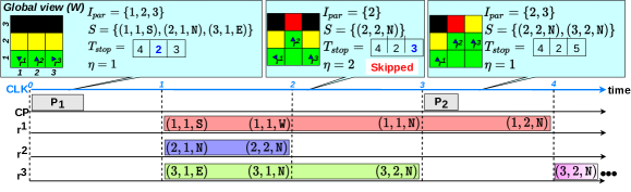
Figure 2: Skip replanning the participants

Example 3

In Figure 2, we show an example where the CP skips replanning a participant due to the unavailability of goals. Initially, all three robots $r^{1},r^{2}$, and $r^{3}$ participate. As there are no non-participants, $\widetilde{W_{g}}=\emptyset$. Moreover, $W_{g}\setminus\widetilde{W_{g}}\neq\emptyset$. So, the first round P₁ begins, where the CP finds paths, timestamped with $1$, of lengths $3,1,$ and $2$, respectively. So, it updates $T_{stop}$ accordingly and sets $\eta=1$ because $r^{2}$ reaches its goal at $CLK=2$, which is the earliest. When $r^{2}$ sends its updated request, the CP cannot start another round because the non-participants’ reserved goals $\widetilde{W_{g}}=\{(1,2),(3,2)\}$ make $W_{g}\setminus\widetilde{W_{g}}=\emptyset$. So, the CP skips replanning $r^{2}$ (line 22 of Algorithm 2) and increments $\eta$ to $2$ because $r^{3}$’s request arrives at $CLK=3$, which is now the earliest. When $r^{3}$ sends its updated request, a goal becomes available as $\widetilde{W_{g}}=\{(1,2)\}$ make $W_{g}\setminus\widetilde{W_{g}}\neq\emptyset$. So, P₂ begins for $r^{2}$ and $r^{3}$.

III-C Coverage Path Planning in the current round

ConCPP_Round (lines 29-46) performs two tasks, viz., replanning the participants of the current round (line 30) and dynamically setting $\eta$ for the next round (lines 31-44). First, the CP invokes ConCPPForPar (Algorithm 3, discussed in section III-D), which finds the paths $\Sigma=\{\sigma^{i}\ |\ i\in I^{*}_{par}\}$ timestamped with $T_{start}$ for the participants $I^{*}_{par}$. These paths $\Sigma$ must be collision-free w.r.t. the existing paths of the non-participants $\overline{I^{*}_{par}}$, which the CP checks from $\Pi$.

Next, the CP examines $\Sigma$ (lines 31-39) to determine which participants are active (lines 32-35) and which are not (lines 36-39). If a participant $r^{i}$, where $i\in I^{*}_{par}$, is found active (i.e., $|\sigma^{i}|>0$), the CP creates a dummy path $\zeta$, containing $T_{start}-T_{stop}[i]-1$ many $s^{i}_{0}$ state (line 33) because $r^{i}$ halts at $s^{i}_{0}$ for $CLK\in\{(T_{stop}[i]+1),\cdots,(T_{start}-1)\}$ before starting to follow $\sigma^{i}$ from $T_{start}$. Then, it updates $r^{i}$’s full path $\pi^{i}$ with $\zeta$ and $\sigma^{i}$ (line 34). It also updates $T_{stop}[i]$ (line 35) because after following $\sigma^{i}$ from $T_{start}$, $r^{i}$ reaches its goal at $T_{start}+|\sigma^{i}|$ and sends its updated request. In contrast, if $r^{i}$ is found inactive, the CP adds $r^{i}$’s ID $i$ to $I_{par}$, its state $s^{i}_{0}$ to $S$, and increments $\eta$ by $1$ (lines 37-39) as it reattempts to find a path for $r^{i}$ in the next round. Thus, inactive participants of the current round become participants in the next round.

As the current round goes on, a non-participant $r^{j}$, where $j\in\overline{I^{*}_{par}}$, sends its request to the CP if it reaches its goal recently, i.e., $T_{stop}[j]\leq CLK$. So, the CP increases $\eta$ for planning their paths in the next round (lines 40-42). At this point (line 43), $\eta$ remains $0$ if all the participants $I^{*}_{par}$ are found active (lines 32-35) and all the non-participants $\overline{I^{*}_{par}}$ (if any) are yet to reach their goals (the implicit else part of the if statement in line 41). So, the CP invokes increment_eta for all the robots (lines 44 and 24-28), which first determines $T_{min}$ (line 25), the earliest $CLK$ value when it will receive new requests, and subsequently sets $\eta$ to the number of requests arriving at $T_{min}$ (lines 26-28). In the penultimate step, the CP invokes $\mathtt{send\_paths\_to\_active\_participants}$ (line 45) that creates a response message $\mathtt{M_{res}}$ containing path $\sigma^{i}$ and timestamp $T_{start}$ for each active participant $r^{i}$, and subsequently sends that $\mathtt{M_{res}}$ to $r^{i}$.

Finally, the CP concludes the current round by invoking check_CPP_criteria (line 46), which checks whether it can start the next round to plan paths for the inactive participants of the current round (lines 36-39), the new participants (lines 40-42), or both. Lines 31-46 constitute a critical section as the CP updates $I_{par},S$, and $\eta$.

Example 4

In Example 2, the CP calls increment_eta (line 44 of Algorithm 2) in $P\textsubscript{2-4, 6}$ but not in $P\textsubscript{1}$ and $P\textsubscript{5}$. In $P\textsubscript{1}$, the CP finds participant $r^{1}$ inactive (line 39) and during $P\textsubscript{5}$ it receives a request from non-participant $r^{3}$ (line 42).

III-D Coverage Path Planning for the Participants

ConCPPForPar (Algorithm 3) finds the participants’ paths $\Sigma$ with timestamp $T_{start}$ in two steps, viz., cost-optimal path finding (line 1) and collision-free path finding (lines 2-11). It is based on Algorithm 3 of [26], which finds only $\Sigma$ while keeping the non-participants’ existing paths intact.

1

2

Result: Participants’ paths $\Sigma$ with timestamp $T_{start}$

3

4$\langle\Gamma,\Phi\rangle\leftarrow\mathtt{COPForPar}(W^{*},\widetilde{W_{g}},I^{*}_{par},S^{*},M)$

$la\leftarrow 1$

  // Number of $CLK$ values to look-ahead

5 while $true$ do

6      $t^{start}_{cur}\leftarrow\mathtt{read\_current\_time()}$

7      $T_{start}\leftarrow CLK+la$

8      $\Sigma_{rem}\leftarrow\mathtt{get\_remaining\_paths}(\overline{I^{*}_{par}},\Pi,T_{start})$

9      $\Sigma\leftarrow\mathtt{CFPForPar}(\Gamma,\Phi,I^{*}_{par},R,\Sigma_{rem})$

10     if $CLK<T_{start}$ then  break

11       // Success else  // Failure! So, Reattempt

12           $t^{end}_{cur}\leftarrow\mathtt{read\_current\_time()}$

13           $la\leftarrow 1+[\lfloor\{t^{end}_{cur}+(t^{end}_{cur}-t^{start}_{cur})\}/\tau\rfloor-CLK]$

14          

15          

Algorithm 3 $\mathtt{ConCPPForPar}(W^{*},\widetilde{W_{g}},I^{*}_{par},S^{*},M,R,\Pi)$

III-D1 Cost-optimal Paths

In the current round, let $R^{*}$ be the number of participants, i.e., $R^{*}=|I^{*}_{par}|=|S^{*}|$ and $G^{*}$ be the number of unassigned goals, i.e., $G^{*}=|W^{*}_{g}\setminus\widetilde{W_{g}}|$. So, the CP finds an assignment $\Gamma$ using the Hungarian algorithm [29] to cost-optimally assign the participants $I^{*}_{par}$ to the unassigned goals having IDs $[G^{*}]$. Formally, $\Gamma:I^{*}_{par}\rightarrow[G^{*}]\cup\{\mathsf{NULL}\}$, where $\Gamma[i]$ denotes the goal ID assigned to a participant $r^{i}$. Note that $\Gamma[i]$ can be $\mathsf{NULL}$, e.g., when $R^{*}>G^{*}$. Such a participant is said to be inactive, whose optimal path $\varphi^{i}$ only contains its current state $s^{i}_{0}$. Otherwise, it is said to be active. Therefore, its optimal path $\varphi^{i}$ leads $r^{i}$ from its current state $s^{i}_{0}$ to the goal having id $\Gamma[i]$ using motions $M$. Such a path $\varphi^{i}$ passes through some cells in $W^{*}_{c}\cup W^{*}_{g}$ but avoids cells in $W^{*}_{o}\cup W^{*}_{u}$. We denote the set of participants’ optimal paths by $\Phi=\{\varphi^{i}\ |\ i\in I^{*}_{par}\}$.

III-D2 Collision-free Paths

The participants’ optimal paths in $\Phi$ are not necessarily collision-free, meaning a participant $r^{i}$, where $i\in I^{*}_{par}$, may collide with another participant $r^{j}$, $j(\neq i)\in I^{*}_{par}$ or a non-participant $r^{k}$, where $k\in\overline{I^{*}_{par}}$. So, the CP must make the participants’ paths collision-free. Moreover, it must find the timestamp $T_{start}$ of those collision-free paths. So, first, the CP sets $T_{start}$ (line 5) to be the next $CLK$ value using a look-ahead $la\in\mathbb{N}$ (line 2).

Next, the CP precisely computes the remaining paths $\Sigma_{rem}=\{\sigma^{k}_{rem}\ |\ k\in\overline{I^{*}_{par}}\}$ of the non-participants starting from $T_{start}$ (line 6) using the following Equation 1.

$$\sigma^{k}_{rem}=\begin{cases}s^{k}_{|\pi^{k}|},&\text{if $|\pi^{k}|\leq T_{start}$}\\ s^{k}_{T_{start}}\ \cdots\ s^{k}_{|\pi^{k}|},&\text{otherwise.}\end{cases}$$ (1)

The remaining path $\sigma^{k}_{rem}$ of a non-participant $r^{k}$, where $k\in\overline{I^{*}_{par}}$, contains the last state of $r^{k}$ in its full path $\pi^{k}$ if $r^{k}$ reaches its goal by $T_{start}$. Otherwise, $\sigma^{k}_{rem}$ contains the remaining part of $\pi^{k}$, which $r^{k}$ is yet to traverse from $T_{start}$.

Now, the CP invokes $\mathtt{CFPForPar}$, which uses the idea of Prioritized Planning to generate the collision-free paths $\Sigma$ for the participants $I^{*}_{par}$ without altering the remaining paths $\Sigma_{rem}$ for the non-participants $\overline{I^{*}_{par}}$. It is a two-step procedure. In the first step, it dynamically prioritizes the participants based on their movement constraints in $\Phi$. For example, if the start location $\mathcal{L}(s^{i}_{0})$ of a participant $r^{i}$ is on the path $\varphi^{j}$ of another participant $r^{j}$, then $r^{i}$ must depart from its start location before $r^{j}$ gets past that location. Similarly, if the goal location $\mathcal{L}(s^{i}_{|\varphi^{i}|})$ of $r^{i}$ is on $\varphi^{j}$ of $r^{j}$, then $r^{j}$ must get past that goal location before $r^{i}$ arrives at that location. The non-participants implicitly have higher priorities than the participants, as the CP does not change $\Sigma_{rem}$. In the last step, it offsets the participants’ paths by prefixing them with $\mathtt{Halt(H)}$ moves in order of their priority to avoid collision with higher priority robots. When a collision between a participant and a non-participant becomes inevitable, it inactivates the participant and returns to the first step. Otherwise, the offsetting step succeeds, and the participants’ paths $\Sigma$ become collision-free. In the worst case, all the participants may get inactivated to avoid collisions with the non-participants during offsetting (see Example 5).

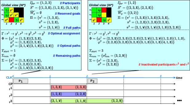
Figure 3: Generating collision-free paths

Example 5

Figure 3 shows an example where only robots $r^{1}$ and $r^{2}$ participate in the planning round P₂. So, the CP finds their optimal paths $\varphi^{1}$ and $\varphi^{2}$, leading them to goals $g^{1}$ and $g^{2}$, respectively. Participant $r^{2}$ has higher priority than $r^{1}$ as $r^{2}$’s start location is on $\varphi^{1}$, meaning $r^{2}$ must leave its start location before $r^{1}$ passes through that location. During offsetting, first, the CP inactivates $r^{2}$ because non-participant $r^{3}$’s remaining path $\sigma^{3}_{rem}$ blocks $\varphi^{2}$. Subsequently, the CP inactivates $r^{1}$ because recently inactivated $r^{2}$ now blocks $\varphi^{1}$.

As the CP timestamps $\Sigma$ with $T_{start}$, an active participant $r^{i}$ must start following its path $\sigma^{i}$ from $T_{start}$. Put differently, $r^{i}$ must receive $\sigma^{i}$ from the CP before $CLK$ becomes $T_{start}$ (line 8). Otherwise, the CP reactively updates $la$ (lines 4 and 9-11) to reattempt with a new $T_{start}$ (line 5).

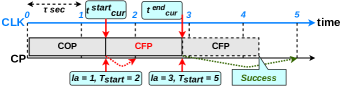
Figure 4: Reattempt to find the participants’ collision-free paths

Example 6

In Figure 4, we show an example where the CP sets $T_{start}$ to $2$ at the beginning of the collision-free pathfinding. As it finishes the computation, $CLK$ is already $2$. Hence, the participants’ paths $\Sigma$ become space-time inconsistent, which the CP cannot send to the participants. So, it updates $la$ to $3$, sets $T_{start}$ to $5$, and reattempts. Now, the CP succeeds in finishing the computation on time.

IV Theoretical Analysis

In this section, first, we formally prove that ConCPP guarantees complete coverage of the unknown workspace $W$. Then, we analyze its time complexity.

IV-A Proof of Complete Coverage

First, we give the outline of the proof. Horizon-based CP [25], in each horizon, replans all the robots and guarantees that at least one robot remains active to visit its goal, which we mention in Lemma 1. Another horizon-based CP [26], in each horizon, replans for only a subset of robots (the participants) on demand. Therefore, in a horizon, if all the robots are participants, i.e., $R^{*}=R$, the latter idea becomes equivalent to the former, which we acknowledge in Lemma 2. As our CP builds upon the on-demand replanning approach of [26], in Lemma 3, we establish the fact that in a round, if all the robots are participants, there is at least one active participant to visit its goal. To prove incremental coverage, in Lemma 4, we establish that rounds where all the robots are participants occur always eventually. Finally, in Theorem 1, we prove that the incremental coverage eventually leads to complete coverage of $W$ when ConCPP terminates.

Lemma 1 (Lemma $4.3$ in [25])

GAMRCPP_Horizon ensures that at least one goal gets visited in each horizon.

Lemma 2 (Lemma $2$ in [26])

CPPForPar $\equiv$ GAMRCPP_Horizon if $R^{*}=R$.

Lemma 3

In a round, ConCPPForPar $\equiv$ CPPForPar if all the robots are participants.

Proof:

The difference between ConCPPForPar (Algorithm 3) and CPPForPar (Algorithm 3 in [26]) is that in ConCPPForPar, CFPForPar (line 7) is in a while loop (lines 3-11). In a round, no non-participants exist if all the robots are participants, i.e., $R^{*}=R$. So, the non-participants’ remaining paths $\Sigma_{rem}=\emptyset$ (line 6). As explained in Section III-D2, this while loop iterates at most twice to find the participants’ collision-free paths $\Sigma$, additionally the timestamp $T_{start}$ (lines 7-8). Thus, ConCPPForPar outputs the same $\Sigma$ as CPPForPar does if $R^{*}=R$. Hence, ConCPPForPar $\equiv$ CPPForPar if all the robots are participants. ∎

Lemma 4

Always eventually, there will be a round with all the robots as participants.

Proof:

Initially, the number of intended participants $\eta=R$ (line 2 in Algorithm 2). So, in the initial round, all the robots are participants, i.e., $R^{*}=R$ trivially (line 11). Before the CP invokes ConCPP_Round (line 19), the CP resets $\eta$ (line 18) to reinitialize it at the end of the planning round for replanning inactive participants in the next planning round (line 39). In the worst case, by Lemma 3, 2, and 1, ConCPPForPar finds exactly one participant active in $\Sigma$ (line 30), thereby reinitializing $\eta=R-1$ (line 39) for replanning $R-1$ inactive participants in the next planning round (lines 46 and 11). Moreover, in the worst case, due to the unavailability of unassigned goals, i.e., $W_{g}\setminus\widetilde{W_{g}}=\emptyset$ (line 13), the CP skips replanning $R-1$ participants, invoking increment_eta (line 23) and making $\eta=R$ again, thereby, the only active participant of the previous round also becomes a participant after reaching its goal and sending its updated $\mathtt{M_{req}}$ (lines 5-9). Thus, all the robots become participants again, making $R^{*}=R$ (line 11). Hence, always eventually, there will be a round with all the robots as participants. ∎

Theorem 1

ConCPP eventually stops, and when it stops, it ensures complete coverage of $W$.

Proof:

All the robots are initially participants, i.e., $R^{*}=R$ (lines 2 and 11 in Algorithm 2). So, there are no non-participants, thereby their assigned goals $\widetilde{W_{g}}=\emptyset$ (line 12). Now, if there are no goals, i.e., $W_{g}=\emptyset$, it falsifies the if condition in line 13 and satisfies the if condition in line 20; hence the CP stops. Otherwise, the CP invokes ConCPP_Round (line 19), which by Lemma 3, 2, and 1, finds at least one participant active in $\Sigma$ (line 30). So, while following its path, an active participant explores the unexplored cells $W_{u}$ into either obstacles $W_{o}$ or goals $W_{g}$ (if any) as $W_{free}$ is strongly connected, eventually covering its goal into $W_{c}$. Thus, $W_{c}$ increases. By Lemma 4, always eventually, this planning round keeps occurring, where all the robots are participants, meaning $R^{*}=R$ and $\widetilde{W_{g}}=\emptyset$. Now, if $W_{g}=\emptyset$, the CP stops, which entails $W_{c}=W_{free}$. Otherwise, the CP invokes ConCPP_Round. ∎

IV-B Time Complexity Analysis

We now analyze the time complexity of ConCPP.

Lemma 5 (Lemma $4$ of [26])

The function $\mathtt{CFPForPar}$ takes $\mathcal{O}(R^{3})$.

Lemma 6

The function $\mathtt{COPForPar}$ takes $\mathcal{O}(|W|^{3})$.

Proof:

Please refer to Lemma $5$ of [26]. ∎

Lemma 7

The function ConCPPForPar takes $\mathcal{O}(|W|^{3})$.

Proof:

Finding the remaining paths $\Sigma_{rem}$ of the non-participants $\overline{I^{*}_{par}}$ from $\Pi$ (line 6 in Algorithm 3) takes $\mathcal{O}(R-R^{*})$. By Lemma 5, $\mathtt{CFPForPar}$ (line 7) takes $\mathcal{O}(R^{3})$. The rest of the body of the while loop (lines 3-11) takes $\mathcal{O}(1)$. Furthermore, this loop iterates at most twice, as explained in Section III-D2. So, this loop takes total $\mathcal{O}(2\cdot((R-R^{*})+R^{3}+1))$, which is $\mathcal{O}(R^{3})$ as $R^{*}=\mathcal{O}(R)$. Now, by Lemma 6, $\mathtt{COPForPar}$ (line 1) takes $\mathcal{O}(|W|^{3})$. Also, initialization of $la$ (line 2) takes $\mathcal{O}(1)$. Hence, ConCPPForPar total takes $\mathcal{O}(|W|^{3}+1+R^{3})$, which is $\mathcal{O}(|W|^{3})$ as $R=\mathcal{O}(|W|)$. ∎

Lemma 8

The function increment_eta takes $\mathcal{O}(R)$.

Proof:

The body of the for loop (lines 26-28 in Algorithm 2) takes $\mathcal{O}(1)$ and the loop iterates at most $|I|$ times. So, this loop total takes $\mathcal{O}(|I|)$. Similarly, determining $T_{min}$ (line 25) takes $\mathcal{O}(|I|)$. So, increment_eta total takes $\mathcal{O}(|I|)$, which is $\mathcal{O}(R)$ as $|I|=\mathcal{O}(R)$. ∎

Lemma 9

The function check_CPP_criteria takes $\mathcal{O}(|W|)$.

Proof:

By Lemma 8, increment_eta (line 23 in Algorithm 2) takes $\mathcal{O}(R)$. Likewise, checking whether all the robots are participants (line 20) takes $\mathcal{O}(R^{*})$. So, the if-else block (lines 20-23) takes $\mathcal{O}(R^{*}+(1+R))$, which is $\mathcal{O}(R)$ as $R^{*}=\mathcal{O}(R)$. Now, taking a snapshot of $W$ (line 14) takes $\mathcal{O}(|W|)$. Also, taking snapshots of $I_{par}$ and $S$ (lines 15-16) take $\mathcal{O}(R^{*})$ each. The rest of the body of the if block (lines 14-19) takes $\mathcal{O}(1)$. So, the body of this block total takes $\mathcal{O}(|W|+R^{*}+1)$. Next, checking whether there exists any unassigned goal (line 13) takes $\mathcal{O}(|W|)$. Therefore, the if-else if-else block (lines 13-23) total takes $\mathcal{O}(|W|+((|W|+R^{*}+1)+R))$, which is $\mathcal{O}(|W|+R)$. Next, computing the reserved goals $\widetilde{W_{g}}$ for the non-participants $\overline{I_{par}}$ from $\Pi$ (line 12) takes $\mathcal{O}(R-R^{*})$ and checking whether there are $\eta$ participants (line 11) takes $\mathcal{O}(R^{*})$. Hence, check_CPP_criteria total takes $\mathcal{O}(R^{*}+((R-R^{*})+(|W|+R)))$, which is $\mathcal{O}(|W|)$. ∎

Lemma 10

The function ConCPP_Round takes $\mathcal{O}(|W|^{3})$.

Proof:

By Lemma 7, ConCPPForPar (line 30) takes $\mathcal{O}(|W|^{3})$. The body of the first for loop (lines 31-39) takes $\mathcal{O}(1)$, and it iterates $R^{*}$ times. So, this loop total takes $\mathcal{O}(R^{*})$. Similarly, the body of the second for loop (lines 40-42) takes $\mathcal{O}(1)$, and it iterates $R-R^{*}$ times. So, this loop total takes $\mathcal{O}(R-R^{*})$. By Lemma 8, increment_eta (line 44) takes $\mathcal{O}(R)$. So, the if block (lines 43-44) takes $\mathcal{O}(R)$. Next, parallelly sending timestamped paths to the active participants (line 45) takes $\mathcal{O}(1)$. Finally, by Lemma 9, check_CPP_criteria (line 46) takes $\mathcal{O}(|W|)$. Hence, ConCPP_Round total takes $\mathcal{O}(|W|^{3}+R^{*}+(R-R^{*})+R+1+|W|)$, which is $\mathcal{O}(|W|^{3})$. ∎

Lemma 11

The function receive_localview takes $\mathcal{O}(|W|^{2})$.

Proof:

Adding a participant’s $\mathtt{id}$ to $I_{par}$ (line 6 in Algorithm 2) and $\mathtt{state}$ to $S$ (line 7) take $\mathcal{O}(1)$ each. Also, updating the global view $W$ with the participant’s local view $W^{i}$ (line 8) takes $\mathcal{O}(|W|^{2})$ (please refer to Theorem $2$ of [26]). By Lemma 9, check_CPP_criteria (line 9) takes $\mathcal{O}(|W|)$. Hence, receive_localview total takes $\mathcal{O}(1+|W|^{2}+|W|)$, which is $\mathcal{O}(|W|^{2})$. ∎

Theorem 2

Time complexity of ConCPP is $\mathcal{O}(|W|^{4})$.

Proof:

The initialization block (lines 1-4 in Algorithm 2) takes $\mathcal{O}(R)$. In the worst case, by Lemma 4, a planning round where all the robots participate keeps exactly one participant active and the rest inactive. So, that active participant follows its path, reaches its goal, and then sends its updated request to receive_localview (line 5), which by Lemma 11, takes $\mathcal{O}(|W|^{2})$. Additionally, ConCPP_Round gets invoked (line 19), which by Lemma 10, takes $\mathcal{O}(|W|^{3})$. Overall it needs $\mathcal{O}(|W_{g}|)$ such rounds, amounting to total $\mathcal{O}(R+(|W_{g}|\cdot(|W|^{2}+|W|^{3})))$, which is $\mathcal{O}(|W|^{4})$ as $|W_{g}|=\mathcal{O}(|W|)$. ∎

V Evaluation

V-A Implementation and Experimental Setup

We implement $\mathtt{Robot}$ (Algorithm 1) and ConCPP (Algorithm 2) in a common ROS [30] C++ package, which runs in a workstation having Intel^® Xeon^® Gold 6226R Processor and 48 GB of RAM, and running Ubuntu $22.04.4$ LTS OS.

V-A1 Workspaces for experimentation

We consider eight large $2$D grid benchmark workspaces of varying size and obstacle density from [31].

V-A2 Robots for experimentation

We consider multiple TurtleBots [27] (introduced before) to cover four of the workspaces and Quadcopters (introduced below) for the rest.

Example 7

The state of a quadcopter is $s^{i}_{j}=(x,y)\in W$, which is its location in $W$. So, its set of motions is $M=\{$$\mathtt{Halt(H)}$, $\mathtt{MoveEast(ME)}$, $\mathtt{MoveNorth(MN)}$, $\mathtt{MoveWest(MW)}$, $\mathtt{MoveSouth(MS)}\}$, where $\mathtt{ME}$ moves it to the neighboring cell east of the current cell. Likewise, we define $\mathtt{MN,MW}$ and $\mathtt{MS}$.

For each experiment, we incrementally deploy $R\in\{128,256,512\}$ robots and repeat $10$ times with different random initial deployments to report their mean in performance metrics. We take a robot’s path cost as the number of moves performed, where each takes $\tau=1$\mathrm{s}$$ for execution.

V-A3 Performance metrics

We consider the mission time ($T_{m}$) as the performance metric to compare proposed ConCPP with OnDemCPP, which is horizon-based, i.e., in each horizon, the path planning and the path following interleave. So, in OnDemCPP, $T_{m}=T_{c}+T_{p}$, where $T_{c}$ and $T_{p}$ are the total computation time and the total path following time, respectively, across all horizons. Note that $T_{p}=\Lambda\times\tau$, where $\Lambda$ is the path length, which is equal for all the robots. However, both can overlap in an interval (duration between consecutive $CLK$ values) in ConCPP. Hence, in ConCPP, $T_{m}$ is the duration from the beginning till complete coverage gets attained, where $T_{c}$ is the total computation time across all rounds and $\Lambda$ is the final $CLK$ value when the coverage gets completed.

V-B Results and Analysis

We show the experimental results in Table I, where we list the workspaces in increasing order of the number of obstacle-free cells ($|W_{free}|$) for each type of robot.

V-B1 Achievement in parallelizing path planning and path following

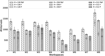
Figure 5: Decomposition of #Intervals

In Figure 5, we show the decomposition of the number of intervals (i.e., the final $CLK$ value) needed to attain the complete coverage into the number of intervals where both path planning and path following happened, only path following happened, and only path planning happened, which we abbreviate as P&F, F, and P, respectively. It shows the power of the proposed approach, parallelizing the path planning with the path following in $55-89\%$ of the intervals. Further, it shows that #Intervals decreases as the number of robots ($R$) increases, completing the coverage faster.

V-B2 Performance of ConCPPForPar (Algorithm 3)

The CP invokes ConCPPForPar in each round (line 30 in Algorithm 2) to find the participants’ timestamped paths. As $R$ increases, both the number of participants per round $R^{*}$ (fourth column in Table I) and the number of nonparticipants per round $R-R^{*}$ increase. So, Figure 6 shows that the mean computation time per round ($\mu_{c}$), comprising of the mean cost-optimal path finding time ($\mu_{COP}$) and the mean collision-free path finding time ($\mu_{CFP}$), also increases. Recall that the CP spends $\mu_{COP}$ in COPForPar and $\mu_{CFP}$ in CFPForPar (lines 1 and 7, respectively, in Algorithm 3). Moreover, COPForPar is independent of the timestamp $T_{start}$ but CFPForPar is not as the nonparticipants remaining paths $\Sigma_{rem}$ depend on $T_{start}$ (line 6). As $\mu_{CFP}$ increases with $R$, Figure 7 shows that CFPForPar fails to find the participants’ collision-free paths $\Sigma$ on time in merely $0-8\%$ of the rounds (line 9). Therefore, the CP reattempts to find $\Sigma$ in the second iteration of the while loop (lines 3-11). Note that #Rounds decreases with $R$ as more robots complete the coverage faster. Also, the CP runs these rounds in P&F and P intervals. Moreover, #Rounds can be greater than #Intervals as the CP can sequentially run multiple rounds on demand in an interval, as explained in Example 2.

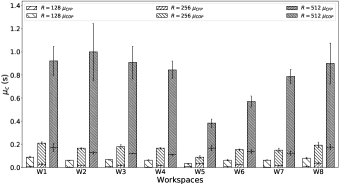
Figure 6: Decomposition of $\mu_{c}$

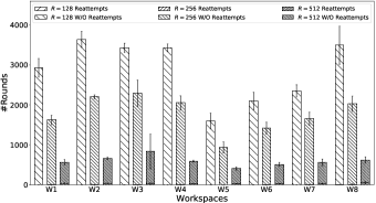
Figure 7: Decomposition of #Rounds

V-B3 Comparison of Mission Time in Table I

TABLE I: Experimental results

				$R^{*}$		$T_{c}\ ($\mathrm{s}$)$		$T^{ol}_{c}\ ($\mathrm{s}$)$	$T_{p}\ ($\mathrm{s}$)$		$T_{non-Halt}\ ($\mathrm{s}$)$		$T_{m}\ ($\mathrm{s}$)$		Mission
$M$	Workspace		$R$	OnDemCPP	ConCPP	OnDemCPP	ConCPP	ConCPP	OnDemCPP	ConCPP	OnDemCPP	ConCPP	OnDemCPP	ConCPP	Speed Up
Quadcopter	W1: w_woundedcoast $578\times 642\ (34,020)$		128	080.4 $\pm$ 3.8	33.8 $\pm$ 03.0	410.1 $\pm$ 058.4	265.3 $\pm$ 40.6	264.4 $\pm$ 40.6	1042.0 $\pm$ 149.5	1358.0 $\pm$ 135.2	554.5 $\pm$ 46.3	610.5 $\pm$ 56.6	1452.1 $\pm$ 167.1	1358.2 $\pm$ 135.2	1.1
			256	170.7 $\pm$ 5.7	82.6 $\pm$ 05.3	579.2 $\pm$ 150.2	344.2 $\pm$ 53.7	340.9 $\pm$ 54.0	804.2 $\pm$ 250.9	962.0 $\pm$ 197.7	291.9 $\pm$ 52.1	310.9 $\pm$ 31.5	1383.4 $\pm$ 383.0	962.1 $\pm$ 197.7	1.4
			512	361.5 $\pm$ 9.7	233.9 $\pm$ 13.2	639.5 $\pm$ 168.6	512.8 $\pm$ 61.2	506.1 $\pm$ 60.8	557.2 $\pm$ 138.9	891.0 $\pm$ 183.1	153.0 $\pm$ 19.8	206.2 $\pm$ 33.3	1196.7 $\pm$ 255.4	891.0 $\pm$ 183.1	1.3
	W2: Paris_1_256 $256\times 256\ (47,240)$		128	081.3 $\pm$ 2.6	30.3 $\pm$ 01.8	332.5 $\pm$ 037.8	222.3 $\pm$ 023.7	222.2 $\pm$ 023.7	962.6 $\pm$ 100.8	1371.6 $\pm$ 149.4	664.3 $\pm$ 41.0	696.5 $\pm$ 39.6	1295.1 $\pm$ 118.8	1371.7 $\pm$ 149.4	0.9
			256	157.2 $\pm$ 3.7	62.6 $\pm$ 01.7	618.5 $\pm$ 079.6	363.3 $\pm$ 015.3	362.9 $\pm$ 015.5	656.2 $\pm$ 049.4	965.8 $\pm$ 024.9	383.1 $\pm$ 08.7	399.5 $\pm$ 03.2	1274.7 $\pm$ 110.8	965.9 $\pm$ 024.9	1.3
			512	335.6 $\pm$ 7.0	194.4 $\pm$ 13.4	992.2 $\pm$ 113.6	658.0 $\pm$ 139.1	657.2 $\pm$ 139.3	455.7 $\pm$ 050.1	929.0 $\pm$ 146.5	208.5 $\pm$ 13.1	258.3 $\pm$ 18.0	1447.9 $\pm$ 117.1	929.1 $\pm$ 146.6	1.6
	W3: Berlin_1_256 $256\times 256\ (47,540)$		128	083.2 $\pm$ 02.5	31.9 $\pm$ 01.7	296.2 $\pm$ 017.2	225.4 $\pm$ 012.1	224.0 $\pm$ 013.1	898.2 $\pm$ 063.9	1334.0 $\pm$ 049.1	625.2 $\pm$ 25.1	658.4 $\pm$ 30.3	1194.4 $\pm$ 065.0	1334.1 $\pm$ 049.1	0.9
			256	167.4 $\pm$ 12.1	80.8 $\pm$ 23.1	598.9 $\pm$ 069.8	417.9 $\pm$ 096.2	371.1 $\pm$ 035.8	669.6 $\pm$ 048.9	1186.8 $\pm$ 275.0	368.5 $\pm$ 13.3	389.1 $\pm$ 19.1	1268.5 $\pm$ 103.3	1186.9 $\pm$ 275.0	1.1
			512	365.2 $\pm$ 34.5	259.8 $\pm$ 87.4	947.8 $\pm$ 115.1	713.8 $\pm$ 280.3	637.5 $\pm$ 159.5	524.9 $\pm$ 140.0	1075.6 $\pm$ 381.5	200.0 $\pm$ 07.2	232.7 $\pm$ 13.1	1472.7 $\pm$ 238.9	1075.7 $\pm$ 381.5	1.4
	W4: Boston_0_256 $256\times 256\ (47,768)$		128	079.6 $\pm$ 4.5	30.8 $\pm$ 00.8	313.3 $\pm$ 030.1	217.8 $\pm$ 12.4	217.6 $\pm$ 12.4	928.0 $\pm$ 100.6	1334.8 $\pm$ 102.1	665.3 $\pm$ 47.8	681.8 $\pm$ 34.0	1241.3 $\pm$ 116.3	1334.9 $\pm$ 102.1	0.9
			256	157.8 $\pm$ 9.3	66.9 $\pm$ 04.3	531.7 $\pm$ 061.2	339.8 $\pm$ 37.9	338.2 $\pm$ 38.4	625.9 $\pm$ 046.9	949.8 $\pm$ 029.7	373.8 $\pm$ 29.9	382.1 $\pm$ 30.7	1157.6 $\pm$ 092.4	949.9 $\pm$ 029.7	1.2
			512	345.3 $\pm$ 7.7	187.0 $\pm$ 10.2	718.1 $\pm$ 119.3	501.8 $\pm$ 34.1	499.0 $\pm$ 34.6	428.7 $\pm$ 069.2	847.6 $\pm$ 058.4	191.9 $\pm$ 15.7	222.4 $\pm$ 08.2	1146.8 $\pm$ 182.2	847.7 $\pm$ 058.4	1.4
TurtleBot	W5: maze-128-128-2 $128\times 128\ (10,858)$		128	075.5 $\pm$ 7.4	47.8 $\pm$ 08.6	76.8 $\pm$ 19.8	50.1 $\pm$ 12.2	50.0 $\pm$ 12.2	791.5 $\pm$ 202.1	874.6 $\pm$ 89.7	281.6 $\pm$ 46.7	294.8 $\pm$ 14.0	868.3 $\pm$ 217.7	874.7 $\pm$ 89.7	0.9
			256	174.7 $\pm$ 7.5	111.6 $\pm$ 14.7	97.5 $\pm$ 16.9	85.4 $\pm$ 24.5	85.3 $\pm$ 24.5	417.6 $\pm$ 097.4	489.8 $\pm$ 71.4	122.7 $\pm$ 16.4	144.8 $\pm$ 09.8	515.1 $\pm$ 113.7	489.9 $\pm$ 71.4	1.1
			512	378.4 $\pm$ 6.8	301.8 $\pm$ 35.8	155.5 $\pm$ 23.9	156.1 $\pm$ 40.4	155.5 $\pm$ 40.3	224.3 $\pm$ 032.1	293.4 $\pm$ 55.7	58.3 $\pm$ 03.3	65.2 $\pm$ 05.5	379.8 $\pm$ 054.1	293.5 $\pm$ 55.7	1.3
	W6: den520d $257\times 256\ (28,178)$		128	071.9 $\pm$ 3.2	31.4 $\pm$ 02.6	191.5 $\pm$ 17.7	133.6 $\pm$ 24.8	133.6 $\pm$ 24.8	773.1 $\pm$ 106.9	991.0 $\pm$ 96.4	486.9 $\pm$ 36.6	494.6 $\pm$ 42.2	964.6 $\pm$ 117.7	991.1 $\pm$ 96.4	0.9
			256	153.8 $\pm$ 3.7	68.0 $\pm$ 02.2	307.6 $\pm$ 63.1	217.0 $\pm$ 36.2	216.4 $\pm$ 36.3	506.4 $\pm$ 057.4	715.8 $\pm$ 37.9	259.3 $\pm$ 11.3	291.0 $\pm$ 25.4	814.0 $\pm$ 103.4	715.9 $\pm$ 37.9	1.1
			512	331.1 $\pm$ 6.6	200.4 $\pm$ 18.9	384.9 $\pm$ 29.2	292.7 $\pm$ 39.5	292.2 $\pm$ 39.4	398.6 $\pm$ 037.9	519.4 $\pm$ 40.9	145.6 $\pm$ 06.1	167.0 $\pm$ 08.4	783.5 $\pm$ 051.7	519.5 $\pm$ 40.9	1.5
	W7: warehouse-20-40-10-2-2 $164\times 340\ (38,756)$		128	081.2 $\pm$ 2.6	27.4 $\pm$ 01.5	260.7 $\pm$ 22.2	151.2 $\pm$ 12.4	151.1 $\pm$ 12.4	707.6 $\pm$ 082.5	1018.8 $\pm$ 059.8	520.3 $\pm$ 25.6	544.5 $\pm$ 13.2	968.3 $\pm$ 098.3	1018.9 $\pm$ 059.8	0.9
			256	149.3 $\pm$ 8.1	57.1 $\pm$ 06.6	401.5 $\pm$ 31.2	250.4 $\pm$ 55.6	249.3 $\pm$ 55.4	502.5 $\pm$ 078.2	772.2 $\pm$ 063.4	319.6 $\pm$ 14.7	337.7 $\pm$ 35.4	904.0 $\pm$ 100.4	772.3 $\pm$ 063.4	1.2
			512	335.5 $\pm$ 7.2	216.2 $\pm$ 16.1	473.7 $\pm$ 36.6	440.4 $\pm$ 82.3	439.6 $\pm$ 82.3	375.2 $\pm$ 029.5	684.0 $\pm$ 111.9	170.3 $\pm$ 09.3	199.3 $\pm$ 26.6	848.9 $\pm$ 054.7	684.1 $\pm$ 111.9	1.2
	W8: brc202d $481\times 530\ (43,151)$		128	065.1 $\pm$ 3.5	25.9 $\pm$ 02.3	467.7 $\pm$ 070.7	288.4 $\pm$ 53.2	288.1 $\pm$ 53.2	1444.9 $\pm$ 232.0	1764.2 $\pm$ 241.4	857.4 $\pm$ 78.1	917.7 $\pm$ 162.8	1912.6 $\pm$ 273.6	1764.3 $\pm$ 241.4	1.1
			256	142.0 $\pm$ 8.7	56.1 $\pm$ 06.8	790.1 $\pm$ 152.3	398.1 $\pm$ 80.3	396.1 $\pm$ 80.3	972.5 $\pm$ 147.1	1413.2 $\pm$ 091.9	461.5 $\pm$ 62.3	565.7 $\pm$ 029.6	1762.6 $\pm$ 230.3	1413.3 $\pm$ 091.9	1.2
			512	309.6 $\pm$ 9.5	215.7 $\pm$ 16.6	818.2 $\pm$ 112.5	546.3 $\pm$ 43.0	544.8 $\pm$ 42.9	780.9 $\pm$ 098.5	1030.2 $\pm$ 119.8	266.2 $\pm$ 29.8	297.3 $\pm$ 022.6	1599.1 $\pm$ 163.1	1030.3 $\pm$ 119.8	1.6

First, the number of participants per planning round $R^{*}$ increases with $R$ as more robots become participants. In OnDemCPP, inactive participants of the current horizon participate again in the next horizon with the new participants, who reach their goals in the current horizon. However, in ConCPP, the next planning round starts instantly even if $I_{par}$ contains only one participant, which could be an inactive participant of the current round or a new participant (lines 36-39 or 40-42 in Algorithm 2). So, $R^{*}$ is lesser in ConCPP.

Next, the total computation time $T_{c}$ increases with $R$ because in each round, finding cost-optimal paths and subsequently collision-free paths for $R^{*}$ participants while respecting $R-R^{*}$ non-participants’ paths become intensive as Figure 6 shows. As $R^{*}$ is lesser in ConCPP. $T_{c}$ is also lesser in ConCPP. Out of $T_{c}$, the total computation time that overlaps with the path following in P&F intervals is denoted by $T^{ol}_{c}$, which is $81-99\%$ of $T_{c}$. The results indicate that almost all the computations have happened in parallel, with at least one robot following its path. It strongly establishes the strength of the concurrent CPP framework.

Now, the total path following time $T_{p}$ decreases with $R$ as more robots complete the coverage faster. In a horizon of OnDemCPP, active robots that do not reach their goals but only progress also send their updated local views to the CP, making the global view more information-rich. So, in the next horizon, the CP finds a superior goal assignment for the participants. In contrast, in ConCPP, active robots send their updated local views to the CP after reaching their goals, keeping the global view less information-rich. It results in inferior goal assignment, leading the participants to distant unassigned goals, making $\Lambda$ relatively longer and so $T_{p}$.

ConCPP gains in terms of $T_{c}$ but losses in terms of $T_{p}$. Despite that, efficient overlapping of path plannings with executions makes ConCPP take shorter mission time $T_{m}$ than OnDemCPP, thereby achieving a speedup of up to $1.6\times$.

V-B4 Significance in Energy Consumption

A quadcopter remains airborne during the entire $T_{m}$ and keeps consuming energy. As ConCPP completes the mission up to $1.6\times$ faster than OnDemCPP, it requires the quadcopters to spend significantly less energy during the mission. Out of $T_{p}$, the TurtleBots spent $T_{non-Halt}$ time (eighth column in Table I) in executing non-$\mathtt{Halt}$ moves while the rest are spent on $\mathtt{Halt}$ moves, which get prefixed to the paths during collision avoidance. In OnDemCPP, a TurtlBot stays idle during $T_{Halt}+T_{c}$ and saves energy. $T_{non-Halt}$ is larger in ConCPP than in OnDemCPP by $1-22\%$. So, the TurtleBots spent more energy in ConCPP. Generally, the energy consumption is less severe an issue for the ground robots than the Quadcopters.

V-C Simulations and Real Experiments

For validation, we perform Gazebo [32] simulations on six $2$D benchmark workspaces from [31] with $10$ IRIS quadcopters and $10$ TurtleBot3 robots, respectively. We also demonstrate two real experiments (see Figure 8) - one outdoor with three quadcopters and one indoor with two TurtleBot2 robots. We equip each quadcopter with a Cube Orange for autopilot, a Here$3$ GPS for localization, and a HereLink Air Unit for communication with the Remote Controller. We equip each TurtleBot2 robot with $4$ HC SR$04$ ultrasonic sound sensor for obstacle detection in the Vicon [33]-enabled indoor workspace for localization. These experimental videos are available as supplementary material.

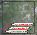
(a) $10\times 10$         outdoor workspace                                 [cell size = $5$\mathrm{m}$$]

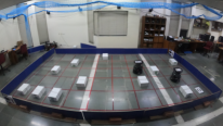
(b) $\phantom{0}5\times 10$ indoor workspace                 [cell size = $0.61$\mathrm{m}$$]

Figure 8: Workspaces for the real experiments

VI Conclusion

We have proposed a non-horizon-based centralized online multi-robot CP, where path planning and path execution happen concurrently. This overlapping saves significant time in completing coverage of large workspaces with hundreds of robots, thereby achieving a speedup of up to $1.6\times$ compared to its horizon-based counterpart. We have also validated the CP by performing simulations and real experiments.

References

- [1] R. Bormann, F. Jordan, J. Hampp, and M. Hägele, “Indoor coverage path planning: Survey, implementation, analysis,” in ICRA, 2018, pp. 1718–1725.
- [2] W. Jing, J. Polden, C. F. Goh, M. Rajaraman, W. Lin, and K. Shimada, “Sampling-based coverage motion planning for industrial inspection application with redundant robotic system,” in IROS, 2017, pp. 5211–5218.
- [3] A. Barrientos, J. Colorado, J. del Cerro, A. Martinez, C. Rossi, D. Sanz, and J. Valente, “Aerial remote sensing in agriculture: A practical approach to area coverage and path planning for fleets of mini aerial robots,” J. Field Robotics, vol. 28, no. 5, pp. 667–689, 2011.
- [4] N. Karapetyan, J. Moulton, J. S. Lewis, A. Q. Li, J. M. O’Kane, and I. M. Rekleitis, “Multi-robot dubins coverage with autonomous surface vehicles,” in ICRA, 2018, pp. 2373–2379.
- [5] T. M. Cabreira, L. B. Brisolara, and P. R. F. Jr., “Survey on coverage path planning with unmanned aerial vehicles,” Drones, vol. 3, no. 1, p. 4, 2019.
- [6] Y. Gabriely and E. Rimon, “Spanning-tree based coverage of continuous areas by a mobile robot,” in ICRA, 2001, pp. 1927–1933.
- [7] A. Kleiner, R. Baravalle, A. Kolling, P. Pilotti, and M. Munich, “A solution to room-by-room coverage for autonomous cleaning robots,” in IROS, 2017, pp. 5346–5352.
- [8] G. Sharma, A. Dutta, and J. Kim, “Optimal online coverage path planning with energy constraints,” in AAMAS, 2019, pp. 1189–1197.
- [9] J. Modares, F. Ghanei, N. Mastronarde, and K. Dantu, “UB-ANC planner: Energy efficient coverage path planning with multiple drones,” in ICRA, 2017, pp. 6182–6189.
- [10] N. Karapetyan, K. Benson, C. McKinney, P. Taslakian, and I. M. Rekleitis, “Efficient multi-robot coverage of a known environment,” in IROS, 2017, pp. 1846–1852.
- [11] I. Vandermeulen, R. Groß, and A. Kolling, “Turn-minimizing multirobot coverage,” in ICRA, 2019, pp. 1014–1020.
- [12] G. Hardouin, J. Moras, F. Morbidi, J. Marzat, and E. M. Mouaddib, “Next-best-view planning for surface reconstruction of large-scale 3D environments with multiple uavs,” in IROS, 2020, pp. 1567–1574.
- [13] L. Collins, P. Ghassemi, E. T. Esfahani, D. S. Doermann, K. Dantu, and S. Chowdhury, “Scalable coverage path planning of multi-robot teams for monitoring non-convex areas,” in ICRA, 2021, pp. 7393–7399.
- [14] J. Tang, C. Sun, and X. Zhang, “Mstc: Multi-robot coverage path planning under physical constrain,” in ICRA, 2021, pp. 2518–2524.
- [15] E. Galceran and M. Carreras, “A survey on coverage path planning for robotics,” Robotics and Autonomous Systems, vol. 61, no. 12, pp. 1258–1276, 2013.
- [16] Y. Bouzid, Y. Bestaoui, and H. Siguerdidjane, “Quadrotor-uav optimal coverage path planning in cluttered environment with a limited onboard energy,” in IROS, 2017, pp. 979–984.
- [17] X. Chen, T. M. Tucker, T. R. Kurfess, and R. W. Vuduc, “Adaptive deep path: Efficient coverage of a known environment under various configurations,” in IROS, 2019, pp. 3549–3556.
- [18] B. Yamauchi, “Frontier-based exploration using multiple robots,” in AGENTS, K. P. Sycara and M. J. Wooldridge, Eds., 1998, pp. 47–53.
- [19] N. Hazon, F. Mieli, and G. A. Kaminka, “Towards robust on-line multi-robot coverage,” in ICRA, 2006, pp. 1710–1715.
- [20] A. Özdemir, M. Gauci, A. Kolling, M. D. Hall, and R. Groß, “Spatial coverage without computation,” in ICRA, 2019, pp. 9674–9680.
- [21] M. Dharmadhikari, T. Dang, L. Solanka, J. Loje, H. Nguyen, N. Khedekar, and K. Alexis, “Motion primitives-based path planning for fast and agile exploration using aerial robots,” in ICRA, 2020, pp. 179–185.
- [22] S. N. Das and I. Saha, “Rhocop: Receding horizon multi-robot coverage,” in ICCPS, 2018.
- [23] H. H. Viet, V. Dang, S. Y. Choi, and T. Chung, “BoB: an online coverage approach for multi-robot systems,” Appl. Intell., vol. 42, no. 2, pp. 157–173, 2015.
- [24] A. Bircher, M. Kamel, K. Alexis, H. Oleynikova, and R. Siegwart, “Receding horizon “next-best-view” planner for 3D exploration,” in ICRA, 2016, pp. 1462–1468.
- [25] R. Mitra and I. Saha, “Scalable online coverage path planning for multi-robot systems,” in IROS, 2022, pp. 10 102–10 109.
- [26] ——, “Online on-demand multi-robot coverage path planning,” CoRR, vol. abs/2303.00047, 2023, accepted at ICRA 2024. [Online]. Available: https://arxiv.org/abs/2303.00047
- [27] TurtleBot. [Online]. Available: https://www.turtlebot.com/
- [28] J. Eidson, IEEE 1588-2019 - IEEE Standard for a Precision Clock Synchronization Protocol for Networked Measurement and Control Systems, IEEE SA Std., 2020.
- [29] H. W. Kuhn, “The hungarian method for the assignment problem,” Nav. Res. Logist., vol. 2, no. 1-2, pp. 83–97, 1955.
- [30] Robot Operating System. [Online]. Available: https://www.ros.org/
- [31] R. Stern, N. R. Sturtevant, A. Felner, S. Koenig, H. Ma, T. T. Walker, J. Li, D. Atzmon, L. Cohen, T. K. S. Kumar, E. Boyarski, and R. Bartak, “Multi-agent pathfinding: Definitions, variants, and benchmarks,” Symposium on Combinatorial Search (SoCS), pp. 151–158, 2019.
- [32] Gazebo. [Online]. Available: https://www.gazebosim.org/
- [33] Vicon Motion Capture Systems. [Online]. Available: https://www.vicon.com/