Stationary non-radial localized patterns in the planar Swift-Hohenberg PDE: constructive proofs of existence

Abstract

In this paper, we present a methodology for establishing constructive proofs of existence of smooth, stationary, non-radial localized patterns in the planar Swift-Hohenberg equation. Specifically, given an approximate solution $u_{0}$, we construct an approximate inverse for the linearization around $u_{0}$, enabling the development of a Newton-Kantorovich approach. Consequently, we derive a sufficient condition for the existence of a unique localized pattern in the vicinity of $u_{0}$. The verification of this condition is facilitated through a combination of analytic techniques and rigorous numerical computations. Moreover, an additional condition is derived, establishing that the localized pattern serves as the limit of a family of periodic solutions (in space) as the period tends to infinity. The integration of analytical tools and meticulous numerical analysis ensures a comprehensive validation of this condition. To illustrate the efficacy of the proposed methodology, we present computer-assisted proofs for the existence of three distinct unbounded branches of periodic solutions in the planar Swift-Hohenberg equation, all converging towards a localized planar pattern, whose existence is also proven constructively. All computer-assisted proofs, including the requisite codes, are accessible on GitHub at [1].

Key words. Localized stationary planar patterns, Swift-Hohenberg PDE, Newton-Kantorovich method, Branches of periodic orbits, Computer-Assisted Proofs

AMS Subject Classification. 35B36, 35K57, 65N35, 65T40, 46B45, 47H10

1 Introduction

In this paper, we investigate the existence (and local uniqueness) of smooth, stationary, non-radial localized patterns in the planar Swift-Hohenberg (SH) equation [2]

$$u_{t}=-\left((I_{d}+\Delta)^{2}u+\mu u+\nu_{1}u^{2}+\nu_{2}u^{3}\right)\stackrel{{\scriptstyle\mbox{\tiny{\raisebox{0.0pt}[0.0pt][0.0pt]{def}}}}}{{=}}-\mathbb{F}(u),\quad u=u(x,t),\leavevmode\nobreak\ \leavevmode\nobreak\ x\in{\mathbb{R}}^{2},$$ (1)

where $\mu,\nu_{2}>0$ and $\nu_{1}<0$ are given parameters and where $\mathbb{F}(u)=\mathbb{L}u+\mathbb{G}(u)$ with

$$\mathbb{L}u\stackrel{{\scriptstyle\mbox{\tiny{\raisebox{0.0pt}[0.0pt][0.0pt]{def}}}}}{{=}}(I_{d}+\Delta)^{2}u+\mu u,\qquad\mathbb{G}(u)\stackrel{{\scriptstyle\mbox{\tiny{\raisebox{0.0pt}[0.0pt][0.0pt]{def}}}}}{{=}}\nu_{1}u^{2}+\nu_{2}u^{3}.$$ (2)

The SH equation is a well-established partial differential equation (PDE) model for pattern formation which finds applications in fields as diverse as phase-field crystals [3], magnetizable fluids [4] and nonlinear optics [5]. Its noteworthy feature of generating localized patterns, often in the form of spatially confined structures, offers valuable insights into the underlying dynamics and stability of complex systems. The existence and dynamics of localized patterns in (1) have been extensively studied in the past decades (e.g. see [6] or [7] for an introduction to the subject). Comprehensive mathematical analysis, complemented by numerical experiments, has played a pivotal role in revealing the complexities inherent in the pattern formation process within the SH equation (1). Notably, homoclinic snaking [8, 9], coupled with bifurcation theory [10, 11, 12], and careful numerical simulations, has significantly enhanced our understanding of the formation of symmetric planar patterns, such as hexagonal [13, 14], radial [10, 15, 16], stripe [13] and square [17] patterns. Moreover, leveraging the reversibility of the equation and its first integral, proofs of localized patterns can be derived under certain hypotheses [18]. Specifically, for $\mu$ small in (1), several existence results have been obtained using bifurcation arguments, allowing for the proof of existence of branches of patterns with $\mu\in(0,\mu^{*})$, for some $\mu^{*}>0$, using the implicit function theorem or fixed-point theorems. Some examples of such proofs may be found in articles such as [18, 19, 20, 15, 13, 10, 14]. Finally, without assuming $\mu$ small, a proof existence of a radially symmetric planar pattern in (1) was recently proposed in [21] by solving a projected boundary value problem a using a rigorous enclosure of a local center-stable manifold.

In general, establishing the existence of stationary patterns for PDEs defined on unbounded domains, without imposing assumptions on parameters or constraining symmetries (e.g. radial), is a notoriously difficult task. Notably, the analytical intricacies diverge significantly from the bounded case due to the loss of compactness in the resolvent of differential operators. The present paper addresses these challenges within the context of the SH equation (1), presenting a general (computer-assisted) method to constructively prove the existence of planar non-radial localized patterns. This result is, to the best of our knowledge, both new and novel.

Our methodology builds upon the framework established in [22], and it crucial to underscore that certain modifications are required to examine equation (1) defined on ${\mathbb{R}}^{2}$, as elaborated later. The method first relies upon the availability of a numerical approximation, denoted as $u_{0}$, known on a square ${\Omega_{0}}=(-d,d)^{2}$. Additionally, $u_{0}$ is required to belong to a Hilbert space of smooth functions on ${\mathbb{R}}^{2}$, exhibiting vanishing behavior at infinity. To meet this criterion, a specific Hilbert space, denoted as $H^{l}_{D_{2}}$, is introduced as a subset of $H^{4}(\mathbb{R}^{2})$ (see (7)). Elements in $H^{l}_{D_{2}}$ possess $D_{2}$-symmetry, signifying invariance under reflection about the $x$ and $y$ axes. This symmetry serves to isolate solutions by eliminating natural translation and rotation invariance. It is noteworthy that the constraint to $D_{2}$-symmetric solutions is not the exclusive means of isolating solutions (see Remark 2.1). However, for the purposes of simplifying the analysis and reducing computational complexity, our focus here is on $D_{2}$-symmetry. Supposing $u_{0}\in H^{l}_{D_{2}}$, the objective is to identify a solution $\tilde{u}\in H^{l}_{D_{2}}$ of equation (1) in proximity to $u_{0}$. This involves the construction of an approximate inverse $\mathbb{A}$ for the Fréchet derivative $D\mathbb{F}(u_{0})$ and the formulation of a fixed-point operator $\mathbb{T}$ defined as $\mathbb{T}(u)=u-\mathbb{A}\mathbb{F}(u)$. Employing a Newton-Kantorovich approach, the aim is to demonstrate that $\mathbb{T}:\overline{B_{r}(u_{0})}\to\overline{B_{r}(u_{0})}$ is a contraction mapping on a closed ball $\overline{B_{r}(u_{0})}$ centered at $u_{0}$. This, in turn, enables the conclusion that a unique solution to (1) exists in $H^{l}_{D_{2}}$ close to $u_{0}$, as guaranteed by the Banach fixed-point theorem. Figure 1 illustrates three distinct approximate solutions $u_{0}$ for which proofs of existence of localized patterns were successfully obtained via the approach just described. The specific details of these proofs are presented in Theorems 4.1, 4.2 and 4.3. Notably, the well-definedness and contractivity of $\mathbb{T}$ are rigorously verified throughout the explicit computation of various upper bounds, as detailed in Section 3.

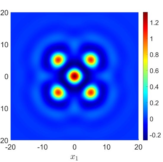
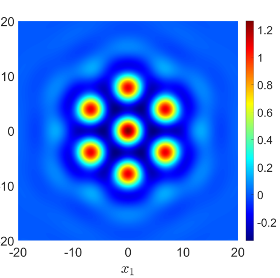
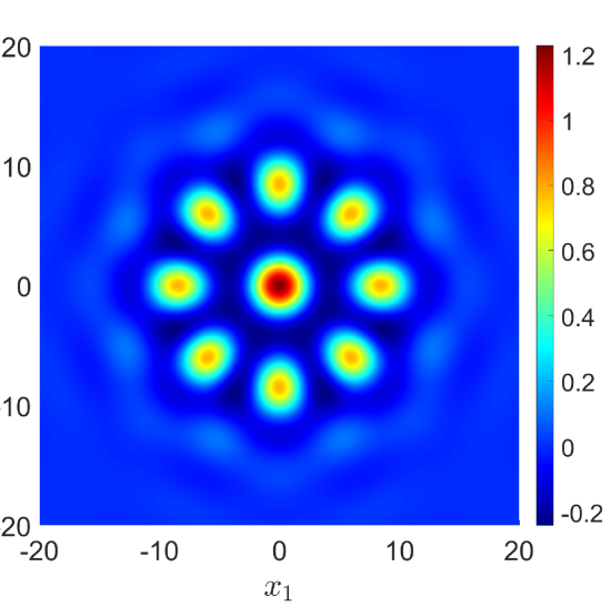
Figure 1: Visualizations of the square pattern (L), hexagonal pattern (C), and octagonal pattern (R), respectively corresponding to Theorems 4.1, 4.2 and 4.3

As previously mentioned, the application of the framework proposed in [22] to the present problem necessitates addressing several technical challenges. The methodology stipulates that the approximate solution $u_{0}$ should be constructed on the domain ${\Omega_{0}}$ through its Fourier coefficients representation $U_{0}$. Beyond the domain ${\Omega_{0}}$, $u_{0}$ is extended to the zero function. Practical implementation involves the numerical computation of the Fourier coefficients $U_{0}$, achieved in this paper utilizing the approach developed in [23]. It is noteworthy that due to the potential discontinuities at $\partial{\Omega_{0}}$, the constructed $u_{0}$ may not be inherently smooth. Specifically, the obtained Fourier coefficients must be projected into the kernel of a periodic trace operator to ensure the smoothness of $u_{0}$ (at least in $H^{4}({\mathbb{R}}^{2})$). The detailed construction of the approximate solution $u_{0}$ is elucidated in Section 3.1. Subsequently, our Newton-Kantorovich approach relies on explicit computations of certain upper bounds (i.e. $\mathcal{Y}_{0},\mathcal{Z}_{1}$ and $\mathcal{Z}_{2}$ in Theorem 3.1). In particular, leveraging the techniques from [22], we provide formulas for these bounds in the case of the SH equation (1). Once established, the explicit evaluation of these formulas is attained through rigorous numerical methods, enabling the verification of the existence of a localized pattern by confirming the condition (34) in Theorem 3.1. Note that a particularly intricate challenge addressed in this study is the precise computation of an upper bound $\hat{C}_{0}$ on the supremum $C_{0}$ of a known smooth function $g:[0,\infty)\to\mathbb{C}$ (see (77)). While various methods, including integral and sum estimates, exist for such computations, analytic techniques often fail to provide a sharp bound, or at the very least, do not furnish means for verifying the sharpness of the bound. Consequently, we employ a rigorous computational approach to tackle this issue, the details of which are explained in Section 3.5.1.

A conjecture advanced in [24] states that localized patterns in the quintic SH equation may manifest as the limit of a family of periodic solutions as their period approaches infinity. The authors of [24] proved the existence of multiple 1D periodic solutions and observed that when parameterized by the period, they seemed to converge to a homoclininic connection (localized pattern on the real line). The present work provides the means to verify such a claim for a given planar localized pattern. Assuming the successful establishment of the existence of a localized pattern using the approach outlined earlier, we extend the findings from [22]. Specifically, we derive a condition on the bounds $\mathcal{Y}_{0},\mathcal{Z}_{1}$ and $\mathcal{Z}_{2}$ under which an unbounded branch of (spatially) periodic solutions is obtained, converging to the localized pattern as the period tends to infinity. This phenomenon is exemplified and demonstrated in Theorems 4.1, 4.2 and 4.3, where we establish the existence of such a branch for three distinct localized patterns. This contribution represents, to the best of our knowledge, a novel result within the domain of localized solutions in semi-linear PDEs.

Before proceeding any further, it is worth mentioning that the use of computer-assisted proofs (CAPs) has by now established itself as an important tool in the analysis of nonlinear PDEs (e.g. refer to [25, 26, 27, 28] and the book [29]), especially in the analysis of (1). For instance, the novel approach of [30] considered (1) on an interval and combined Conley index theory with CAPs of existence of steady states to build a model for the attractor consisting of stationary solutions and connecting orbits. In [31], a proof of existence of chaos in the form of symbolic dynamics in the stationary SH equation on the line was obtained by combining a CAP of a skeleton of periodic solutions, parabolic relations, braid theory and a topological forcing theorem. Shortly after, in [32, 33], the authors considers the SH equation on 2D/3D rectangular domains with periodic boundary conditions, where they developed analytic estimates in weighted $\ell^{\infty}$ spaces of Fourier coefficients and used a Newton-Kantorovich type theorem to obtain constructive proofs of existence of steady states. Still on bounded domains, the recent construction [34] of stable manifolds of equilibria in (1) and the recent works [35, 36, 37] based on Fourier-Chebyshev expansions for solving initial value problems opened the door to rigorous computations of connecting orbits in (1). In the case of unbounded domains, a constructive proof of existence of a radial localized pattern in (1) was recently proposed in [21]. By studying the equation in polar coordinates, the 2D PDE transforms into an ordinary differential equation (ODE), for which a homoclinic connection at zero is computed via a rigorous enclosure of the center stable manifold, achieved through the use of the Lyapunov-Perron operator. Concurrently, [23] delved into the examination of the SH equation (1) with polar coordinates, where their focus was on identifying solutions characterized by a finite expansion in the angle component, giving rise to a finite system of ODEs in the radial component. This system underwent rigorous resolution employing a finite-dimensional Newton-Kantorovich argument.

Finally, it is noteworthy to highlight that, although the number of outcomes is limited, there is a gradual emergence of computer-assisted methodologies in investigating PDEs on unbounded domains. Indeed, as mentioned earlier, the loss of compactness in the resolvent of differential operators for PDEs defined on unbounded domains hinders significantly the analysis. Consequently, the development of CAPs for PDEs defined on unbounded domains requires special care. It is worth mentioning that for problems posed on the 1D line, the Parameterization Method, as exemplified in [38, 39], provides a means to formulate a projected boundary value problem solvable through Chebyshev series or splines, as detailed in [40, 41]. While this methodology facilitates the constructive establishment of solutions and provide efficiently the asymptotic dynamics in the stable and unstable manifolds, it however lacks a generalization to “fully” 2D PDEs, thereby precluding its applicability to the study of planar localized patterns. In [29], Plum et al. present a comprehensive methodology for proving weak solutions to second and fourth-order PDEs. Their approach relies on the rigorous control of the spectrum of the linearization around an approximate solution, incorporating a homotopy argument and the Temple-Lehmann-Goerisch method. Notably, this approach is applicable to unbounded domains, as demonstrated by the authors in establishing the existence of a weak solution to the planar Schrödinger equation. Within the same theoretical framework, Wunderlich, in [42], successfully demonstrated the existence of a weak solution to the Navier-Stokes equations defined on an infinite strip with an obstacle. It is essential to highlight, however, that the approach presented in [29] exclusively enables the verification of weak solutions on unbounded domains and does not provide regularity. In our current work, we adopt the framework proposed in [22] and employ it to formulate a general methodology for proving constructively the existence of strong solutions in (1) in the form of planar localized stationary patterns.

The paper is organized as follows. Section 2 introduces the problem’s framework, provides a comprehensive exposition of the setup and introduces the definition of pertinent operators and spaces essential to our investigation. In Section 3, a Newton-Kantorovich approach is introduced for the rigorous constructive proof of existence of localized patterns, outlining the methodology for obtaining and constructing an approximate solution within the space $H^{l}_{D_{2}}$. Additionally, explicit computations leading to bounds required by this approach are detailed. Finally, Section 4 is devoted to the presentation of proofs regarding the existence of localized patterns. All computer-assisted proofs, including the requisite codes, are accessible on GitHub at [1].

2 Set-up of the problem

In this section, we recall some set-up developed in [22] and present it in the specific context of the planar Swift-Hohenberg equation. Recall the Lebesgue notation $L^{2}=L^{2}(\mathbb{R}^{2})$ and $L^{2}(\Omega_{0})$ on a bounded domain ${\Omega_{0}}$ in ${\mathbb{R}}^{2}$. More generally, $L^{p}$ denotes the usual $p$ Lebesgue space on $\mathbb{R}^{2}$ associated to its norm $\|\cdot\|_{p}$. Moreover, given $s\in{\mathbb{R}}$, denote by $H^{s}\stackrel{{\scriptstyle\mbox{\tiny{\raisebox{0.0pt}[0.0pt][0.0pt]{def}}}}}{{=}}H^{s}({\mathbb{R}}^{2})$ the usual Sobolev space on ${\mathbb{R}}^{2}$. For a bounded linear operator $\mathbb{K}:L^{2}\to L^{2}$, denote by $\mathbb{K}^{*}$ the adjoint of $\mathbb{K}$ in $L^{2}$. Moreover, if $v\in L^{2}$, denote by $\hat{v}\stackrel{{\scriptstyle\mbox{\tiny{\raisebox{0.0pt}[0.0pt][0.0pt]{def}}}}}{{=}}\mathcal{F}(v)$ the Fourier transform of $v$, that is

$$\hat{v}(\xi)\stackrel{{\scriptstyle\mbox{\tiny{\raisebox{0.0pt}[0.0pt][0.0pt]{def}}}}}{{=}}\int_{\mathbb{R}^{2}}v(x)e^{-2\pi ix\cdot\xi}dx,$$

for all $\xi\in\mathbb{R}^{2}$, where $x\cdot\xi=x_{1}\xi_{1}+x_{2}\xi_{2}$. Given $\xi\in{\mathbb{R}}^{2}$, denote $|\xi|\stackrel{{\scriptstyle\mbox{\tiny{\raisebox{0.0pt}[0.0pt][0.0pt]{def}}}}}{{=}}\sqrt{\xi_{1}^{2}+\xi_{2}^{2}}$ the usual Euclidean norm on ${\mathbb{R}}^{2}$. Finally, given $u,v\in L^{2}$, we denote $u*v$ the convolution of $u$ and $v$.

We wish to prove the existence (and local uniqueness) of localized stationary solutions of the planar Swift-Hohenberg equation. Equivalently, we look for a real-valued $u$ such that

$$(I_{d}+\Delta)^{2}u+\mu u+\nu_{1}u^{2}+\nu_{2}u^{3}=0$$ (3)

with $u(x)\to 0\text{ as }|x|\to\infty$. Using the notations introduced in [22], denote

$$\mathbb{L}\stackrel{{\scriptstyle\mbox{\tiny{\raisebox{0.0pt}[0.0pt][0.0pt]{def}}}}}{{=}}(I_{d}+\Delta)^{2}+\mu I_{d},$$

where $I_{d}$ represents the identity operator and $\Delta$ is the usual Laplacian. Moreover we define $l:\mathbb{R}^{2}\to\mathbb{R}$ as

$$l(\xi)\stackrel{{\scriptstyle\mbox{\tiny{\raisebox{0.0pt}[0.0pt][0.0pt]{def}}}}}{{=}}(1-|2\pi\xi|^{2})^{2}+\mu,\quad\text{for all }\xi\in\mathbb{R}^{2}.$$

In other words, $l$ is the symbol associated to the differential operator $\mathbb{L}$, that is $\mathcal{F}\big{(}\mathbb{L}u\big{)}(\xi)=l(\xi)\hat{u}(\xi)$. We also denote

$$\mathbb{G}(u)\stackrel{{\scriptstyle\mbox{\tiny{\raisebox{0.0pt}[0.0pt][0.0pt]{def}}}}}{{=}}{\mathbb{G}}_{2}(u)+{\mathbb{G}}_{3}(u)=\nu_{1}u^{2}+\nu_{2}u^{3}\leavevmode\nobreak\ \leavevmode\nobreak\ \text{ and }\leavevmode\nobreak\ \leavevmode\nobreak\ \mathbb{F}(u)\stackrel{{\scriptstyle\mbox{\tiny{\raisebox{0.0pt}[0.0pt][0.0pt]{def}}}}}{{=}}\mathbb{L}u+\mathbb{G}(u)$$

where ${\mathbb{G}}_{2}(u)=\nu_{1}u^{2}$ and ${\mathbb{G}}_{3}(u)=\nu_{2}u^{3}$. Moreover, we have ${\mathbb{G}}_{2}(u)=\left({\mathbb{G}}^{1}_{2,1}u\right)\left({\mathbb{G}}^{2}_{2,1}u\right)$ where ${\mathbb{G}}^{1}_{2,1}\stackrel{{\scriptstyle\mbox{\tiny{\raisebox{0.0pt}[0.0pt][0.0pt]{def}}}}}{{=}}\nu_{1}I_{d}$ and ${\mathbb{G}}^{2}_{2,1}\stackrel{{\scriptstyle\mbox{\tiny{\raisebox{0.0pt}[0.0pt][0.0pt]{def}}}}}{{=}}I_{d}$ and ${\mathbb{G}}_{3}(u)=\left({\mathbb{G}}^{1}_{3,1}u\right)\left({\mathbb{G}}^{2}_{3,1}u\right)\left({\mathbb{G}}^{3}_{3,1}u\right)$ where ${\mathbb{G}}^{1}_{3,1}\stackrel{{\scriptstyle\mbox{\tiny{\raisebox{0.0pt}[0.0pt][0.0pt]{def}}}}}{{=}}\nu_{2}I_{d}$ and ${\mathbb{G}}^{2}_{3,1}={\mathbb{G}}^{3}_{3,1}=I_{d}$, using the notations of [22]. In particular, we define $g^{p}_{i,k}:{\mathbb{R}}^{2}\to{\mathbb{R}}$ as the Fourier transform of ${\mathbb{G}}^{p}_{i,k}$. More specifically, $g^{1}_{2,1}(\xi)=\nu_{1}$, $g^{1}_{3,1}(\xi)=\nu_{2}$ and $g^{2}_{2,1}(\xi)=g^{2}_{3,1}(\xi)=g^{3}_{3,1}(\xi)=1$ for all $\xi\in{\mathbb{R}}^{2}$. Equation (3) is then equivalent to the zero finding problem $\mathbb{F}(u)=0$ with $u\to 0$ as $|x|\to\infty$. We recall the assumptions from [22] for convenience.

Assumption 1.

Assume that $|l(\xi)|>0$ for all $\xi\in\mathbb{R}^{2}$.

Assumption 2.

For all $i\in\{2,3\}$ and $p\in\{1,\dots,i\}$, define $g_{i}^{p}$ as

$$\mathcal{F}\bigg{(}\mathbb{G}_{i}^{p}(u)\bigg{)}(\xi)=g_{i}^{p}(\xi)\hat{u}(\xi),\quad\text{for all }\xi\in\mathbb{R}^{2},\text{ and assume that }\leavevmode\nobreak\ \frac{g_{i,k}^{p}}{l}\in L^{1}.\vspace{-.2cm}$$

First, notice Assumption 1 is satisfied as we assume $\mu>0$. Moreover, as the functions $g^{p}_{i,k}$ are all constants, Assumption 2 is verified if and only if $\frac{1}{l}\in L^{1}$, which is trivially satisfied as well. Therefore, the analysis derived in [22] is readily applicable to (3).

Denote by $H^{l}$ the following Hilbert space

$$H^{l}\stackrel{{\scriptstyle\mbox{\tiny{\raisebox{0.0pt}[0.0pt][0.0pt]{def}}}}}{{=}}\left\{u\in L^{2}:\int_{\mathbb{R}^{2}}|\hat{u}(\xi)|^{2}|l(\xi)|^{2}d\xi<\infty\right\}$$

associated to its natural inner product $(\cdot,\cdot)_{l}$ and norm defined as

$$(u,v)_{l}\stackrel{{\scriptstyle\mbox{\tiny{\raisebox{0.0pt}[0.0pt][0.0pt]{def}}}}}{{=}}\int_{\mathbb{R}^{2}}\hat{u}(\xi)\overline{\hat{v}(\xi)}|{l}(\xi)|^{2}d\xi\leavevmode\nobreak\ \leavevmode\nobreak\ \text{ and }\leavevmode\nobreak\ \leavevmode\nobreak\ \|u\|_{l}\stackrel{{\scriptstyle\mbox{\tiny{\raisebox{0.0pt}[0.0pt][0.0pt]{def}}}}}{{=}}\|\mathbb{L}u\|_{2}$$ (4)

for all $u,v\in H^{l}.$ Now, to obtain the well-definedness of the operator $\mathbb{G}:H^{l}\to L^{2}$, we need to ensure that $uv\in L^{2}$ and $uvw\in L^{2}$ for all $u,v,w\in H^{l}$. The next lemma provides such a result.

Lemma 2.1.

Let $\kappa>0$ such that $\kappa\geq\|\frac{1}{l}\|_{2}$. Then, for all $u,v,w\in H^{l}$,

$$\|uw\|_{2}\leq\frac{\kappa}{\mu}\|u\|_{l}\|w\|_{l}\leavevmode\nobreak\ \text{ and }\leavevmode\nobreak\ \|uvw\|_{2}\leq\frac{\kappa^{2}}{\mu}\|u\|_{l}\|v\|_{l}\|w\|_{l}.$$ (5)

Proof.

By definition of $l$, we have $\max_{\xi\in{\mathbb{R}}^{2}}\frac{1}{|l(\xi)|}=\frac{1}{\mu}$. Then, similarly as what was achieved in Lemma 2.4 in [22], one can easily prove that $\kappa$ satisfies (5). ∎

In practice, one needs to know explicitly (or at least have an upper bound) for the quantity $\|\frac{1}{l}\|_{2}$ in order to use (5). This is achieved in the next proposition.

Proposition 2.1.

$$\left\|\frac{1}{l}\right\|_{2}^{2}=\frac{2\sqrt{\mu}+(1+\mu)\left(2\pi-2\arctan(\sqrt{\mu})\right)}{8\mu^{\frac{3}{2}}(1+\mu)}.$$ (6)

Proof.

We have,

$$\left\|\frac{1}{l}\right\|_{2}^{2}=\int_{\mathbb{R}^{2}}\frac{1}{\left(\mu+(1-|2\pi\xi|^{2})^{2}\right)^{2}}d\xi=\int_{0}^{\infty}\frac{r}{\left(\mu+(1-r^{2})^{2}\right)^{2}}dr$$

using polar coordinates. Then, using standard integration techniques for rational functions (see [43] for instance), we prove (6). ∎

Using Lemma 2.1, we obtain that the operator $\mathbb{G}$ is smooth from $H^{l}$ to $L^{2}$. This implies that the zero finding problem $\mathbb{F}(u)=0$ is well defined on $H^{l}.$ The condition $u\to 0$ as $|x|\to\infty$ is satisfied implicitly if $u\in H^{l}.$

Now supposing that $u$ is a solution of (3), then any translation and rotation of $u$ is still a solution. Therefore, in order to isolate a particular solution in the set of solutions, we choose to look for solutions that are invariant under reflections about the $x$-axis and the $y$-axis. In other words, we restrict ourselves to $D_{2}$-symmetric solutions. Therefore, we introduce $H^{l}_{D_{2}}\subset H^{l}$ the following Hilbert subspace of $H^{l}$ which takes into account these symmetries :

$$H^{l}_{D_{2}}\stackrel{{\scriptstyle\mbox{\tiny{\raisebox{0.0pt}[0.0pt][0.0pt]{def}}}}}{{=}}\left\{u\in H^{l}:u(x_{1},x_{2})=u(-x_{1},x_{2})=u(x_{1},-x_{2})\text{ for all }x_{1},x_{2}\in\mathbb{R}\right\}.$$ (7)

Similarly, denote by $L^{2}_{D_{2}}$ the Hilbert subspace of $L^{2}$ satisfying the $D_{2}$-symmetry. In particular we notice that if $u\in H^{l}_{D_{2}}$, then $\mathbb{L}u\in L^{2}_{D_{2}}$ and $\mathbb{G}(u)\in L^{2}_{D_{2}}$, hence it is natural to define $\mathbb{L}$ and $\mathbb{G}$ as operators from $H^{l}_{D_{2}}$ to $L^{2}_{D_{2}}$.

Finally, we look for solutions of the following problem

$$\mathbb{F}(u)=0\leavevmode\nobreak\ \leavevmode\nobreak\ \text{ and }\leavevmode\nobreak\ \leavevmode\nobreak\ u\in H^{l}_{D_{2}}.$$ (8)

As we look for classical solutions to (3), we need to ensure that solutions to (8) are smooth. The next proposition provides such a result and, consequently, we may focus our analysis on the zeros of $\mathbb{F}:H^{l}_{D_{2}}\to L^{2}_{D_{2}}$ and obtain the regularity of the solution a posteriori.

Proposition 2.2.

Let $u\in H^{l}_{D_{2}}$ such that $u$ solves (8). Then $u\in H^{\infty}(\mathbb{R}^{2})\bigcap C^{\infty}({\mathbb{R}}^{2})$ and $u$ is a classical solution of (8).

Proof.

The proof is a direct consequence of Proposition 2.5 in [22]. ∎

Finally, denote by $\|\cdot\|_{l,2}$ the operator norm for any bounded linear operator between the two Hilbert spaces $H^{l}_{D_{2}}$ and $L^{2}_{D_{2}}$. Similarly denote by $\|\cdot\|_{l}$, $\|\cdot\|_{2}$ and $\|\cdot\|_{2,l}$ the operator norms for bounded linear operators on $H^{l}_{D_{2}}\to H^{l}_{D_{2}}$, $L^{2}_{D_{2}}\to L^{2}_{D_{2}}$ and $L^{2}_{D_{2}}\to H^{l}_{D_{2}}$ respectively.

Remark 2.1.

By construction, the space $H^{l}_{D_{2}}$ allows eliminating the translation and rotation invariance of the solutions. If one is interested in proving solutions that are not necessarily $D_{2}$-symmetric, one may use the set-up of Section 5 in [22]. Indeed, by appending extra equations and the same number of unfolding parameters, the solution can be isolated again (see [44, 45] for instance).

2.1 Periodic Sobolev spaces

In this section we recall some notations introduced in Section 2.4 of [22]. We define $\Omega_{0}\stackrel{{\scriptstyle\mbox{\tiny{\raisebox{0.0pt}[0.0pt][0.0pt]{def}}}}}{{=}}(-d,d)^{2}$ where $0<d<\infty$. Then, we define

$$\tilde{n}=(\tilde{n}_{1},\tilde{n}_{2})\stackrel{{\scriptstyle\mbox{\tiny{\raisebox{0.0pt}[0.0pt][0.0pt]{def}}}}}{{=}}\left(\frac{n_{1}}{2d},\frac{n_{2}}{2d}\right)\in\mathbb{R}^{2}$$

for all $(n_{1},n_{2})\in\mathbb{Z}^{2}$. Similarly as in the continuous case, we want to restrict to Fourier series representing $D_{2}$-symmetric functions. Given a Fourier series $U=(u_{n})_{n\in\mathbb{Z}^{2}}$ representing a $D_{2}$-symmetric function, $U$ satisfies

$$u_{n_{1},n_{2}}=u_{-n_{1},n_{2}}=u_{n_{1},-n_{2}}\text{ for all }(n_{1},n_{2})\in\mathbb{Z}^{2}.$$ (9)

Therefore, we restrict the indexing of $D_{2}$-symmetric functions to $\mathbb{N}_{0}^{2}$, where

$$\mathbb{N}_{0}^{2}\stackrel{{\scriptstyle\mbox{\tiny{\raisebox{0.0pt}[0.0pt][0.0pt]{def}}}}}{{=}}\left(\mathbb{N}\cup\{0\}\right)^{2},$$

and construct the full series by symmetry if needed. In other words, $\mathbb{N}_{0}^{2}$ is the reduced set associated to the $D_{2}$-symmetry.

Let $(\alpha_{n})_{n\in\mathbb{N}_{0}^{2}}$ be defined as

$$\alpha_{n}\stackrel{{\scriptstyle\mbox{\tiny{\raisebox{0.0pt}[0.0pt][0.0pt]{def}}}}}{{=}}\begin{cases}1&\text{ if }n=(0,0)\\ 2&\text{ if }n_{1}n_{2}=0,\text{ but }n\neq(0,0)\\ 4&\text{ if }n_{1}n_{2}\neq 0\end{cases}$$ (10)

and let $\ell^{p}_{D_{2}}$ denote the following Banach space

$$\ell^{p}_{D_{2}}\stackrel{{\scriptstyle\mbox{\tiny{\raisebox{0.0pt}[0.0pt][0.0pt]{def}}}}}{{=}}\left\{U=(u_{n})_{n\in\mathbb{N}_{0}^{2}}:\leavevmode\nobreak\ \|U\|_{p}\stackrel{{\scriptstyle\mbox{\tiny{\raisebox{0.0pt}[0.0pt][0.0pt]{def}}}}}{{=}}\left(\sum_{n\in\mathbb{N}_{0}^{2}}\alpha_{n}|u_{n}|^{p}\right)^{\frac{1}{p}}<\infty\right\}.$$

Note that $\ell^{p}_{D_{2}}$ possesses the same sequences as the usual $p$ Lebesgue space for sequences indexed on $\mathbb{N}_{0}^{2}$ but with a different norm. For the special case $p=2$, $l^{2}_{D_{2}}$ is an Hilbert space on sequences indexed on $\mathbb{N}_{0}^{2}$ and we denote $(\cdot,\cdot)_{2}$ its inner product given by

$$(U,V)_{2}\stackrel{{\scriptstyle\mbox{\tiny{\raisebox{0.0pt}[0.0pt][0.0pt]{def}}}}}{{=}}\sum_{n\in\mathbb{N}_{0}^{2}}\alpha_{n}u_{n}\overline{v_{n}}$$

for all $U=(u_{n})_{n\in\mathbb{N}_{0}^{2}},V=(v_{n})_{n\in\mathbb{N}_{0}^{2}}\in\ell^{2}_{D_{2}}.$ Moreover, for a bounded operator $K:\ell^{2}_{D_{2}}\to\ell^{2}_{D_{2}}$, $K^{*}$ denotes the adjoint of $K$ in $\ell^{2}_{D_{2}}$.

The coefficients $(\alpha_{n})_{n\in\mathbb{N}_{0}^{2}}$ arise naturally when switching from the usual Fourier basis in $e^{2\pi i\tilde{n}\cdot x}$ to the one in $\cos(2\pi\tilde{n}_{1}x_{1})\cos(2\pi\tilde{n}_{2}x_{2})$, which is specific to $D_{2}$-symmetric functions. Indeed, given $(u_{n})_{n\in\mathbb{Z}^{2}}$ satisfying (9), we have

$$\sum_{n\in\mathbb{Z}^{2}}u_{n}e^{2\pi i\tilde{n}\cdot x}=\sum_{n\in\mathbb{N}_{0}^{2}}\alpha_{n}u_{n}\cos(2\pi\tilde{n}_{1}x_{1})\cos(2\pi\tilde{n}_{2}x_{2})$$ (11)

for all $(x_{1},x_{2})\in{\mathbb{R}}^{2}$. Now, similarly as what is done in Section 6 of [22], we define $\gamma:L^{2}_{D_{2}}\to\ell^{2}_{D_{2}}$

$$\left(\gamma(u)\right)_{n}\stackrel{{\scriptstyle\mbox{\tiny{\raisebox{0.0pt}[0.0pt][0.0pt]{def}}}}}{{=}}\frac{1}{|{\Omega_{0}}|}\int_{\Omega_{0}}u(x)e^{-2\pi i\tilde{n}\cdot x}dx$$ (12)

for all $n\in\mathbb{N}_{0}^{2}$. Similarly, we define $\gamma^{\dagger}:\ell^{2}_{D_{2}}\to L^{2}_{D_{2}}$ as

$$\gamma^{\dagger}(U)(x)\stackrel{{\scriptstyle\mbox{\tiny{\raisebox{0.0pt}[0.0pt][0.0pt]{def}}}}}{{=}}\mathbb{1}_{\Omega_{0}}(x)\sum_{n\in\mathbb{N}_{0}^{2}}\alpha_{n}u_{n}\cos(2\pi\tilde{n}_{1}x_{1})\cos(2\pi\tilde{n}_{2}x_{2})$$ (13)

for all $x=(x_{1},x_{2})\in{\mathbb{R}}^{2}$ and all $U=\left(u_{n}\right)_{n\in\mathbb{N}_{0}^{2}}\in\ell^{2}_{D_{2}}$, where $\mathbb{1}_{\Omega_{0}}$ is the characteristic function on ${\Omega_{0}}$. Given $u\in L^{2}_{D_{2}}$, $\gamma(u)$ represents the Fourier coefficients indexed on $\mathbb{N}_{0}^{2}$ of the restriction of $u$ on ${\Omega_{0}}$. Conversely, given a sequence $U\in\ell^{2}_{D_{2}}$, ${\gamma^{\dagger}}\left(U\right)$ is the function representation of $U$ in $L^{2}_{D_{2}}.$ In particular, notice that ${\gamma^{\dagger}}\left(U\right)(x)=0$ for all $x\notin{\Omega_{0}}.$ Then, recalling similar notations from [22]

$$L^{2}_{D_{2},{\Omega_{0}}} \stackrel{{\scriptstyle\mbox{\tiny{\raisebox{0.0pt}[0.0pt][0.0pt]{def}}}}}{{=}}\left\{u\in L^{2}_{D_{2}}:\text{supp}(u)\subset\overline{{\Omega_{0}}}\right\}$$ (14)

$$H_{D_{2},{\Omega_{0}}}^{l} \stackrel{{\scriptstyle\mbox{\tiny{\raisebox{0.0pt}[0.0pt][0.0pt]{def}}}}}{{=}}\left\{u\in H^{l}_{D_{2}}:\text{supp}(u)\subset\overline{{\Omega_{0}}}\right\}.$$ (15)

Moreover, recall that $\mathcal{B}(L^{2}_{D_{2}})$ (respectively $\mathcal{B}(\ell^{2}_{D_{2}})$) denotes the space of bounded linear operators on $L^{2}_{D_{2}}$ (respectively $\ell^{2}_{D_{2}}$) and denote by $\mathcal{B}_{\Omega_{0}}(L^{2}_{D_{2}})$ the following subspace of $\mathcal{B}(L^{2}_{D_{2}})$

$$\mathcal{B}_{\Omega_{0}}(L^{2}_{D_{2}})\stackrel{{\scriptstyle\mbox{\tiny{\raisebox{0.0pt}[0.0pt][0.0pt]{def}}}}}{{=}}\{\mathbb{K}_{\Omega_{0}}\in\mathcal{B}(L^{2}_{D_{2}}):\mathbb{K}_{\Omega_{0}}=\mathbb{1}_{\Omega_{0}}\mathbb{K}_{\Omega_{0}}\mathbb{1}_{\Omega_{0}}\}.$$ (16)

Finally, define $\Gamma:\mathcal{B}(L^{2}_{D_{2}})\to\mathcal{B}(\ell^{2}_{D_{2}})$ and $\Gamma^{\dagger}:\mathcal{B}(\ell^{2}_{D_{2}})\to\mathcal{B}(L^{2}_{D_{2}})$ as follows

$$\Gamma(\mathbb{K})\stackrel{{\scriptstyle\mbox{\tiny{\raisebox{0.0pt}[0.0pt][0.0pt]{def}}}}}{{=}}\gamma\mathbb{K}{\gamma^{\dagger}}\leavevmode\nobreak\ \leavevmode\nobreak\ \text{ and }\leavevmode\nobreak\ \leavevmode\nobreak\ \Gamma^{\dagger}(K)\stackrel{{\scriptstyle\mbox{\tiny{\raisebox{0.0pt}[0.0pt][0.0pt]{def}}}}}{{=}}\gamma^{\dagger}{K}\gamma$$ (17)

for all $\mathbb{K}\in\mathcal{B}(L^{2}_{D_{2}})$ and all $K\in\mathcal{B}(\ell^{2}_{D_{2}}).$

The maps defined above in (12), (13) and (17) are fundamental in our analysis as they allow to pass from the problem on ${\mathbb{R}}^{2}$ to the one in $\ell^{2}_{D_{2}}$ and vice-versa. Furthermore, we show in the following lemma, which is proven in [22] using Parseval’s identity, that this passage is actually an isometric isomorphism when restricted to the relevant spaces.

Lemma 2.2.

The map $\sqrt{|{\Omega_{0}}|}\gamma:L^{2}_{D_{2},{\Omega_{0}}}\to\ell^{2}_{D_{2}}$ (respectively $\Gamma:\mathcal{B}_{\Omega_{0}}(L^{2}_{D_{2}})\to\mathcal{B}(\ell^{2}_{D_{2}})$) is an isometric isomorphism whose inverse is given by $\frac{1}{\sqrt{|{\Omega_{0}}|}}{\gamma^{\dagger}}:\ell^{2}_{D_{2}}\to L^{2}_{D_{2},{\Omega_{0}}}$ (respectively $\Gamma^{\dagger}:\mathcal{B}(\ell^{2}_{D_{2}})\to\mathcal{B}_{\Omega_{0}}(L^{2}_{D_{2}})$). In particular,

$$\|u\|_{2}=\sqrt{{\Omega_{0}}}\|U\|_{2}\text{ and }\|\mathbb{K}\|_{2}=\|K\|_{2}$$ (18)

for all $u\in L^{2}_{D_{2},{\Omega_{0}}}$ and $\mathbb{K}\in\mathcal{B}_{\Omega_{0}}(L^{2}_{D_{2}})$, and where $U\stackrel{{\scriptstyle\mbox{\tiny{\raisebox{0.0pt}[0.0pt][0.0pt]{def}}}}}{{=}}\gamma(u)$ and ${K}\stackrel{{\scriptstyle\mbox{\tiny{\raisebox{0.0pt}[0.0pt][0.0pt]{def}}}}}{{=}}\Gamma(\mathbb{K})$.

The above lemma not only provides a one-to-one correspondence between the elements in $L^{2}_{D_{2},{\Omega_{0}}}$ (respectively $\mathcal{B}_{\Omega_{0}}(L^{2}_{D_{2}})$) and the ones in $\ell^{2}_{D_{2}}$ (respectively $\mathcal{B}(\ell^{2}_{D_{2}})$) but it also provides an identity on norms. This property is essential in our construction of an approximate inverse in Section 3.3.

Now, we define the Hilbert space $X^{l}$ as

$$X^{l}\stackrel{{\scriptstyle\mbox{\tiny{\raisebox{0.0pt}[0.0pt][0.0pt]{def}}}}}{{=}}\left\{U=(u_{n})_{n\in\mathbb{N}_{0}^{2}}:\|U\|_{l}<\infty\right\}$$

where $X^{l}$ is associated to its inner product $(\cdot,\cdot)_{l}$ and norm $\|\cdot\|_{l}$ defined as

$$(U,V)_{l}\stackrel{{\scriptstyle\mbox{\tiny{\raisebox{0.0pt}[0.0pt][0.0pt]{def}}}}}{{=}}\sum_{n\in\mathbb{N}_{0}^{2}}\alpha_{n}u_{n}v_{n}^{*}|l(\tilde{n})|^{2}\leavevmode\nobreak\ \leavevmode\nobreak\ \text{ and }\leavevmode\nobreak\ \leavevmode\nobreak\ \|U\|_{l}\stackrel{{\scriptstyle\mbox{\tiny{\raisebox{0.0pt}[0.0pt][0.0pt]{def}}}}}{{=}}\sqrt{(U,U)_{l}}$$

for all $U=(u_{n})_{n\in\mathbb{N}_{0}^{2}},\leavevmode\nobreak\ V=(v_{n})_{n\in\mathbb{N}_{0}^{2}}\in X^{l}.$

Denote by $L:X^{l}\to\ell^{2}_{D_{2}}$ and $G:X^{l}\to\ell^{2}_{D_{2}}$ the Fourier series representation of $\mathbb{L}$ and $\mathbb{G}$ respectively. More specifically, $L$ is represented by an infinite diagonal matrix with coefficients $\left(l(\tilde{n})\right)_{n\in\mathbb{N}_{0}^{2}}$ on the diagonal and $G(U)=\nu_{1}U*U+\nu_{2}U*U*U$, where $U*V\stackrel{{\scriptstyle\mbox{\tiny{\raisebox{0.0pt}[0.0pt][0.0pt]{def}}}}}{{=}}\gamma\left(\gamma^{\dagger}\left(U\right)\gamma^{\dagger}\left(V\right)\right)$ is defined as the discrete convolution (under the $D_{2}$-symmetry) for all $U=(u_{n})_{n\in\mathbb{N}_{0}^{2}}$, and $V=(v_{n})_{n\in\mathbb{N}_{0}^{2}}\in X^{l}$. In particular, notice that Young’s convolution inequality is applicable and

$$\|U*V\|_{2}\leq\|U\|_{2}\|V\|_{1}$$ (19)

for all $U\in\ell^{2}_{D_{2}}$ and all $V\in\ell^{1}_{D_{2}}$.

We define $F(U)\stackrel{{\scriptstyle\mbox{\tiny{\raisebox{0.0pt}[0.0pt][0.0pt]{def}}}}}{{=}}LU+G(U)$ and introduce

$$F(U)=0\leavevmode\nobreak\ \leavevmode\nobreak\ \text{ and }\leavevmode\nobreak\ \leavevmode\nobreak\ U\in X^{l}$$ (20)

as the periodic equivalent on ${\Omega_{0}}$ of (8).

Remark 2.2.

In terms of group theory, $\mathbb{N}^{2}_{0}$ is the reduced set associated to the group of symmetries $D_{2}.$ Moreover, given $n\in\mathbb{N}_{0}^{2}$, $\alpha_{n}$ is the size of the orbit associated to $n.$

3 Computer-assisted analysis

In this section we present our computer-assisted approach to obtain the proofs of existence of localized patterns of (3). More specifically, we first expose the numerical construction of the approximate solution $u_{0}\in H^{l}_{D_{2}}$, such that supp$(u_{0})\subset\overline{{\Omega_{0}}}$, and its associated Fourier series representation $U_{0}\in X^{l}$. The construction is based on the theory developed in [22] (Section 4.1) combined with the numerical analysis derived in [23]. Then, following the set-up introduced in [22], we provide the required technical details for the specific case of the Swift-Hohenberg equation.

Let us first fix $N,N_{0}\in\mathbb{N}$ such that $N_{0}>N$, where $N_{0}$ represents the size of our Fourier series approximation and $N$ the size of the operator approximation. Moreover, given $\mathcal{N}\in\mathbb{N}$, we introduce the projection operators from [22]

$$\left(\pi^{\mathcal{N}}(V)\right)_{n}=\begin{cases}v_{n},&n\in I^{\mathcal{N}}\\ 0,&n\notin I^{\mathcal{N}}\end{cases}\leavevmode\nobreak\ \leavevmode\nobreak\ \text{ and }\leavevmode\nobreak\ \leavevmode\nobreak\ \left(\pi_{\mathcal{N}}(V)\right)_{n}=\begin{cases}0,&n\in I^{\mathcal{N}}\\ v_{n},&n\notin I^{\mathcal{N}}\end{cases}$$ (21)

for all $n\in\mathbb{N}_{0}^{2}$ and $V=(v_{n})_{n\in\mathbb{N}_{0}^{2}}\in\ell^{2}_{D_{2}}$, where $I^{\mathcal{N}}\stackrel{{\scriptstyle\mbox{\tiny{\raisebox{0.0pt}[0.0pt][0.0pt]{def}}}}}{{=}}\{n\in\mathbb{N}_{0}^{2}:0\leq n_{1},n_{2}\leq\mathcal{N}\}$. In particular $U_{0}$ is chosen such that $U_{0}=\pi^{N_{0}}U_{0}$, meaning that $U_{0}$ only has a finite number of non-zero coefficients ($U_{0}$ may be seen as a vector).

Remark 3.1.

The use of two sizes of numerical truncation $N$ and $N_{0}$ allows us to avoid numerical-memory limitations. More specifically, we represent the numerical operators (such as $B^{N}$ defined in Section 3.3) on a truncation of size $N$, which can be different than the truncation of size $N_{0}$ that we use for sequences (such as $U_{0}$ for instance). Since operators are more memory consuming than sequences, it makes sense to choose $N_{0}>N$ in practice. As a consequence, we develop the analysis of the bounds $\mathcal{Y}_{0},$ $\mathcal{Z}_{1},$ and $\mathcal{Z}_{2}$ with different values for $N_{0}$ and $N$ such that $N_{0}>N$.

3.1 Construction of $u_{0}$

The analysis developed in [22] is based on the construction of a fixed point operator around an approximate solution $u_{0}\in H^{l}_{D_{2}}$ such that supp$(u_{0})\subset\overline{{\Omega_{0}}}$. This point constitutes one of the main challenge of this work. To answer this problem, we use the approach developed in Section 4 of [22]. Specifically, we need to compute a Fourier series $U_{0}\in X^{l}$ having a function representation on ${\Omega_{0}}$ with a zero trace of order 4. Finally, we require $U_{0}$ to be finite-dimensional, that is $U_{0}=\pi^{N_{0}}U_{0}$. In other terms, $U_{0}$ has a finite number of non-zero coefficients. This last point is required to perform a computer-assisted proof as $u_{0}$ will possess a representation on the computer.

Following the set-up of [23], we first study the Swift-Hohenberg equation (3) in its radial form on the disk $D_{R}\subset\mathbb{R}^{2}$ centered at zero and of radius $R>0$, that is

$$\left(I_{d}+\partial_{rr}+\frac{\partial_{r}}{r}+\frac{\partial_{\theta\theta}}{r^{2}}\right)^{2}v+\mu v+\nu_{1}v^{2}+\nu_{2}v^{3}=0$$ (22)

and we look for an approximate solution of the form

$$v(\theta,r)=\sum_{n=0}^{N_{1}}v_{n}(r)\cos(sn\theta)$$ (23)

where $v_{n}:(0,R)\to\mathbb{R}$, $N_{1}\in\mathbb{N}$ and $s\in\mathbb{N}$ is a parameter determining the symmetry we want our approximate solution to have (e.g. $s=6$ for hexagonal patterns). Plugging the ansatz (23) into (22), we notice that the functions $(v_{n})$ satisfy a system of ODEs given in Equation (2.6) in [23]. Using a Galerkin projection, we obtain a system of $N_{1}+1$ ODEs with $N_{1}+1$ unknown radial functions. Therefore, instead of solving a PDE on a 2D bounded domain, we reduce the problem to solving a system of ODEs on the interval $(0,R)$. As we look for solutions with the $D_{2}$-symmetry, we impose Neumann’s boundary conditions at $0$.

Then we represent each $v_{n}$ on a grid defined on $(0,R)$ and solve the system of ODEs using a finite-difference scheme combined with the solver fsolve on Matlab. After convergence of fsolve, we construct a grid on $D_{R}$ and obtain an approximate solution at the points of the grid. We use this construction in order to construct a Fourier series representation of the function. In other words, we need to compute the Fourier coefficients

$$\frac{1}{|{\Omega_{0}}|}\int_{\Omega_{0}}v(x)e^{-2\pi i\tilde{n}\cdot x}dx$$

for all $n\in\mathbb{N}_{0}^{2}.$ Supposing that $v$ decreases fast enough to $0$ and that $R$ and $d$ are large enough, then

$$\frac{1}{|{\Omega_{0}}|}\int_{\Omega_{0}}v(x)e^{-2\pi i\tilde{n}\cdot x}dx\approx\frac{1}{|{\Omega_{0}}|}\int_{D_{R}}v(x)e^{-2\pi i\tilde{n}\cdot x}dx.$$

Using a numerical quadrature (trapezoidal rule), we estimate the Fourier series using the values of the function on the disk and obtain a first sequence of Fourier coefficients $\tilde{U}_{0}$ such that $\tilde{U}_{0}=\pi^{N_{0}}\tilde{U}_{0}$. To gain precision, we consider $\tilde{U}_{0}$ as an initial guess for Newton’s method applied to the Galerkin projection ${F}^{N_{0}}:{\mathbb{R}}^{(N_{0}+1)^{2}}\to{\mathbb{R}}^{(N_{0}+1)^{2}}$ defined as

$$\left({F}^{N_{0}}(V)\right)_{n}\stackrel{{\scriptstyle\mbox{\tiny{\raisebox{0.0pt}[0.0pt][0.0pt]{def}}}}}{{=}}\left(F(\iota^{N_{0}}(V))\right)_{n},\qquad n\in I^{N_{0}}$$

where $\iota^{N_{0}}:{\mathbb{R}}^{(N_{0}+1)^{2}}\to\pi^{N_{0}}\ell^{2}$ is the natural inclusion. Once Newton’s method has reached a desired tolerance, we obtain an improved approximation which we still denote by $\tilde{U}_{0}$. In this process, we choose a number of Fourier coefficients $N_{0}\in\mathbb{N}$ big enough in order for the last coefficients of $\tilde{U}_{0}$ to be of the order of machine precision.

At this point, $\tilde{U}_{0}$ represents a $D_{2}$-symmetric function $\tilde{u}_{0}$ in $L^{2}(\Omega_{0})$ and by extending $\tilde{u}_{0}$ by zero outside of ${\Omega_{0}}$, we obtain a function in $L^{2}_{D_{2}}$, but not necessarily in $H^{l}_{D_{2}}.$ To fix this lack of regularity we use the approach presented in Section 4.1 of [22]. More specifically, we need to ensure that $\tilde{u}_{0}$ has a null trace of order 4 so that its extension by zero becomes a function in $H^{4}({\mathbb{R}}^{2})$. Notice first that because $\tilde{u}_{0}$ is smooth on ${\Omega_{0}}$ and has a cosine series representation of the form (11), then its first and third order normal derivatives are automatically zero on $\partial{\Omega_{0}}.$ Therefore, it remains to ensure that $\tilde{u}_{0}$ and its second order normal derivative vanish on $\partial{\Omega_{0}}.$

Let $m\in\{1,2\}$ and define $X^{N_{0},m}$ as the following vector space

$$X^{N_{0},m}\stackrel{{\scriptstyle\mbox{\tiny{\raisebox{0.0pt}[0.0pt][0.0pt]{def}}}}}{{=}}\{(u_{n})_{\mathbb{N}_{0}^{m}}:u_{n}=0\text{ for all }|n|_{\infty}>N_{0}\}$$ (24)

where $|n|_{\infty}=\max_{i\in\{1,\dots,m\}}|n_{i}|$ for all $n\in\mathbb{N}_{0}^{m}.$ In particular, notice that $\tilde{U}_{0}\in X^{N_{0},2}$ by construction. Now, let $H^{N_{0},m}$ be defined as follows

$$H^{N_{0},1} \stackrel{{\scriptstyle\mbox{\tiny{\raisebox{0.0pt}[0.0pt][0.0pt]{def}}}}}{{=}}\left\{u\in L^{2}\left((-d,d)\right):\leavevmode\nobreak\ u(x)=u_{0}+{2}\sum_{n=1}^{N_{0}}u_{n}\cos\left(\frac{\pi nx}{d}\right)\text{ with }(u_{n})_{n\in\mathbb{N}_{0}}\in\ell^{2}(\mathbb{N}_{0})\right\}$$

$$H^{N_{0},2} \stackrel{{\scriptstyle\mbox{\tiny{\raisebox{0.0pt}[0.0pt][0.0pt]{def}}}}}{{=}}\left\{u\in L^{2}\left({\Omega_{0}}\right):\leavevmode\nobreak\ u(x)=\sum_{n\in I^{N_{0}}}u_{n}\alpha_{n}\cos\left(\frac{\pi n_{1}x_{1}}{d}\right)\cos\left(\frac{\pi n_{2}x_{2}}{d}\right)\text{ with }(u_{n})_{n\in\mathbb{N}_{0}^{2}}\in\ell^{2}_{D_{2}}\right\},$$

where $\ell^{2}(\mathbb{N}_{0})\stackrel{{\scriptstyle\mbox{\tiny{\raisebox{0.0pt}[0.0pt][0.0pt]{def}}}}}{{=}}\left\{(u_{n})_{n\in\mathbb{N}_{0}},\leavevmode\nobreak\ \sum_{n\in\mathbb{N}_{0}}|u_{n}|^{2}<\infty\right\}.$ Now, let $\widehat{\mathcal{T}}:H^{N_{0},2}\to\left(H^{N_{0},1}\right)^{4}$ be defined as

$$\widehat{\mathcal{T}}(u)\stackrel{{\scriptstyle\mbox{\tiny{\raisebox{0.0pt}[0.0pt][0.0pt]{def}}}}}{{=}}\begin{pmatrix}u(d,\cdot)\\ \partial_{x}^{2}u(d,\cdot)\\ u(\cdot,d)\\ \partial_{y}^{2}u(\cdot,d)\end{pmatrix},$$

which is a trace operator of order 4 on $H^{N_{0},2}$. Note that, using the periodicity of the elements in $H^{N_{0},2}$, it is sufficient to evaluate at $x_{1}=d$ or $x_{2}=d$ in order to control the whole trace on $\partial{\Omega_{0}}$. Then, $\widehat{\mathcal{T}}$ has a representation $\mathcal{T}:X^{N_{0},2}\to\left(X^{N_{0},1}\right)^{4}$ given by

$$\mathcal{T}(U) \stackrel{{\scriptstyle\mbox{\tiny{\raisebox{0.0pt}[0.0pt][0.0pt]{def}}}}}{{=}}\begin{pmatrix}\mathcal{T}_{1,0}(U)\\ \mathcal{T}_{1,2}(U)\\ \mathcal{T}_{2,0}(U)\\ \mathcal{T}_{2,2}(U)\end{pmatrix}$$ (25)

where

$$\left(\mathcal{T}_{1,j}(U)\right)_{n_{2}}\stackrel{{\scriptstyle\mbox{\tiny{\raisebox{0.0pt}[0.0pt][0.0pt]{def}}}}}{{=}}\displaystyle\sum_{n_{1}=0}^{N_{0}}(-1)^{n_{1}}\alpha_{n}u_{n_{1},n_{2}}\big{(}\frac{\pi n_{1}}{d}\big{)}^{j}\text{ and }\leavevmode\nobreak\ \left(\mathcal{T}_{2,j}(U)\right)_{n_{1}}\stackrel{{\scriptstyle\mbox{\tiny{\raisebox{0.0pt}[0.0pt][0.0pt]{def}}}}}{{=}}\displaystyle\sum_{n_{2}=0}^{N_{0}}(-1)^{n_{2}}\alpha_{n}u_{n_{1},n_{2}}\big{(}\frac{\pi n_{2}}{d}\big{)}^{j}$$ (26)

for all $(n_{1},n_{2})\in\mathbb{N}_{0}^{2}$. In particular, if $\mathcal{T}(U)=0$, then the function representation of $U$ on ${\Omega_{0}}$ has a null trace of order 4 on $\partial{\Omega_{0}}$. Moreover, notice that $\mathcal{T}$ has a $4(N_{0}+1)$ by $(N_{0}+1)^{2}$ matrix representation where $\mathcal{T}_{i,j}:{\mathbb{R}}^{(N_{0}+1)^{2}}\to{\mathbb{R}}^{N_{0}+1}$. We abuse notation and identify $\mathcal{T}$ by its matrix representation.

Recall that the trace operator is not full rank when defined on a polygon (we refer the interested reader to [46] for a complete study of the trace operator on polygons and polyhedra). In particular, compatibility conditions have to be added in order to ensure the smoothness at the vertices of ${\Omega_{0}}.$ Indeed, let $u\in H^{N_{0},2}$ and denote

$$v_{0}\stackrel{{\scriptstyle\mbox{\tiny{\raisebox{0.0pt}[0.0pt][0.0pt]{def}}}}}{{=}}u(\cdot,d),\quad w_{0}\stackrel{{\scriptstyle\mbox{\tiny{\raisebox{0.0pt}[0.0pt][0.0pt]{def}}}}}{{=}}u(d,\cdot),\quad v_{2}\stackrel{{\scriptstyle\mbox{\tiny{\raisebox{0.0pt}[0.0pt][0.0pt]{def}}}}}{{=}}\partial^{2}_{y}u(\cdot,d)\quad\text{and}\quad w_{2}\stackrel{{\scriptstyle\mbox{\tiny{\raisebox{0.0pt}[0.0pt][0.0pt]{def}}}}}{{=}}\partial^{2}_{x}u(d,\cdot).$$

Then, using [46], the compatibility conditions read

$$v_{0}(d)=w_{0}(d),\quad v_{2}(d)=w_{2}(d),\quad v_{0}^{\prime\prime}(d)=v_{2}(d),\quad\text{and}\quad w_{0}^{\prime\prime}(d)=w_{2}(d).$$ (27)

In particular, since $H^{N_{0},2}\subset C^{\infty}({\Omega_{0}})$, [46] provides that $\widehat{\mathcal{T}}:H^{N_{0},2}\to\tilde{H}$ is surjective, where

$$\tilde{H}\stackrel{{\scriptstyle\mbox{\tiny{\raisebox{0.0pt}[0.0pt][0.0pt]{def}}}}}{{=}}\left\{(v_{0},w_{0},v_{2},w_{2})\in\left(H^{N_{0},1}\right)^{4}:\leavevmode\nobreak\ v_{0},w_{0},v_{2},w_{2}\text{ satisfy }\eqref{eq : compatibility condutions}\right\}.$$

This implies that $\mathcal{T}$ has a 4-dimensional cokernel. Since we wish to build a projection into the kernel of $\mathcal{T}$, we need to build a matrix $M:{\mathbb{R}}^{(N_{0}+1)^{2}}\to{\mathbb{R}}^{4N_{0}}$ having the same kernel as $\mathcal{T}$ but being full rank. In fact, the matrix $M$ can be obtained numerically. Practically, one can remove $4$ rows from $\mathcal{T}$ and denote $M$ the obtained matrix. To verify that $M$ is indeed full rank, one can compute the singular values of $MM^{*}$ using interval arithmetic ([47, 48] for instance) and prove that $MM^{*}$ is invertible. If that is the case, it means that $M$ is full rank and that ${\rm Ker}(M)={\rm Ker}(\mathcal{T})$, where ${\rm Ker}(\cdot)$ denotes the kernel. Assuming we are able to obtain such a matrix $M$, we define $D$ to be the diagonal matrix with entries $\left(\frac{1}{l(\tilde{n})}\right)_{n\in I^{N_{0}}}$ on the diagonal and we build a projection $U_{0}$ of $\tilde{U}_{0}$ in the kernel of ${\mathcal{T}}$ defined as

$$U_{0}\stackrel{{\scriptstyle\mbox{\tiny{\raisebox{0.0pt}[0.0pt][0.0pt]{def}}}}}{{=}}\tilde{U}_{0}-DM^{*}(MDM^{*})^{-1}M\tilde{U}_{0}.$$ (28)

We abuse notation in the above equation as $U_{0}$ and $\tilde{U}_{0}$ are seen as vectors in ${\mathbb{R}}^{(N_{0}+1)^{2}}.$ In practice, this construction is made rigorous using interval arithmetic. Finally, letting $u_{0}\stackrel{{\scriptstyle\mbox{\tiny{\raisebox{0.0pt}[0.0pt][0.0pt]{def}}}}}{{=}}\gamma^{\dagger}(U_{0})$, we have that $u_{0}$ satisfies the $D_{2}$-symmetry with $u_{0}\in H^{4}({\mathbb{R}}^{2}),$ $supp(u_{0})\subset\overline{{\Omega_{0}}},$. Noticing that $H^{l}=H^{4}({\mathbb{R}}^{2})$ by equivalence of norms (since $l(\xi)=\mathcal{O}(|\xi|^{4})$), we obtain that $u_{0}\in H^{l}_{D_{2},{\Omega_{0}}}$.

In the rest of this paper, we assume that $u_{0}\in H^{l}_{D_{2},{\Omega_{0}}}$ and $U_{0}\in X^{l}$ satisfy

$$u_{0}\stackrel{{\scriptstyle\mbox{\tiny{\raisebox{0.0pt}[0.0pt][0.0pt]{def}}}}}{{=}}\gamma^{\dagger}(U_{0})\in H^{l}_{D_{2},{\Omega_{0}}}\leavevmode\nobreak\ \text{ and }\leavevmode\nobreak\ U_{0}=\pi^{N_{0}}U_{0}.$$ (29)

3.2 Newton-Kantorovich approach

In this section we expose our computer-assisted approach, which is based on Newton-Kantorovich arguments. More specifically, the zeros of (8) are turned into fixed points of some contracting operator $\mathbb{T}$ defined below. We define

$$v_{0}\stackrel{{\scriptstyle\mbox{\tiny{\raisebox{0.0pt}[0.0pt][0.0pt]{def}}}}}{{=}}2\nu_{1}u_{0}+3\nu_{2}u_{0}^{2}\leavevmode\nobreak\ \text{ and }\leavevmode\nobreak\ V_{0}\stackrel{{\scriptstyle\mbox{\tiny{\raisebox{0.0pt}[0.0pt][0.0pt]{def}}}}}{{=}}\gamma\left(v_{0}\right)\in X^{l},$$ (30)

where $u_{0}$ satisfies (29). In particular, $D\mathbb{G}(u_{0})=\mathbb{v}_{0}$ is the multiplication operator by $v_{0}$. Recall that $V_{0}$ is by definition the sequence of Fourier coefficients of $v_{0}$ on ${\Omega_{0}}$.

We want to prove that there exists $r>0$ such that $\mathbb{T}:\overline{B_{r}(u_{0})}\to\overline{B_{r}(u_{0})}$ defined as

$$\mathbb{T}(u)\stackrel{{\scriptstyle\mbox{\tiny{\raisebox{0.0pt}[0.0pt][0.0pt]{def}}}}}{{=}}u-{\mathbb{A}}\mathbb{F}(u)$$

is well defined and is a contraction, where ${B_{r}(u_{0})}\subset H^{l}_{D_{2}}$ is the open ball of radius $r$ centered at $u_{0}$. In order to determine a possible value for $r>0$ that would provide the contraction and the well-definedness of $\mathbb{T}$, a standard Newton-Kantorovich type theorem is derived. In particular, we want to build $\mathbb{A}:L^{2}_{D_{2}}\to H^{l}_{D_{2}}$, $\mathcal{Y}_{0},$ $\mathcal{Z}_{1},$ and $\mathcal{Z}_{2}>0$ in such a way that the hypotheses of the following Theorem 3.1 are satisfied.

Theorem 3.1 (Localized patterns).

Let $\mathbb{A}:L^{2}_{D_{2}}\to H^{l}_{D_{2}}$ be a bounded linear operator. Moreover, let $\mathcal{Y}_{0},\mathcal{Z}_{1}$ be non-negative constants and let $\mathcal{Z}_{2}:(0,\infty)\to[0,\infty)$ be a non-negative function such that

$$\|\mathbb{A}\mathbb{F}(u_{0})\|_{l} \leq\mathcal{Y}_{0}$$ (31)

$$\|I_{d}-\mathbb{A}D\mathbb{F}(u_{0})\|_{l} \leq\mathcal{Z}_{1}$$ (32)

$$\|\mathbb{A}\left({D}\mathbb{F}(v)-D\mathbb{F}(u_{0})\right)\|_{l} \leq\mathcal{Z}_{2}(r)r,\leavevmode\nobreak\ \leavevmode\nobreak\ \text{for all }v\in\overline{B_{r}(u_{0})}\text{ and all }r>0.$$ (33)

If there exists $r>0$ such that

$$\frac{1}{2}\mathcal{Z}_{2}(r)r^{2}-(1-\mathcal{Z}_{1})r+\mathcal{Y}_{0}<0\text{ and }\mathcal{Z}_{1}+\mathcal{Z}_{2}(r)r<1,$$ (34)

then there exists a unique $\tilde{u}\in\overline{B_{r}(u_{0})}\subset H^{l}_{D_{2}}$ such that $\mathbb{F}(\tilde{u})=0$.

Proof.

First, using Theorem 3.5 in [22], we obtain that both $\mathbb{A}:L^{2}_{D_{2}}\to H^{l}_{D_{2}}$ and $D\mathbb{F}(u_{0}):H^{l}_{D_{2}}\to L^{2}_{D_{2}}$ have a bounded inverse if $\mathcal{Z}_{1}<1$ (which is the case if (34) is satisfied). The rest of the proof can be found in Theorem 2.15 in [49]. ∎

In practice, $\mathbb{F}(u_{0})$ is supposedly small in norm if $u_{0}$ is a good approximation of a solution. The bound $\mathcal{Y}_{0}$ controls the accuracy of this approximation. Since the construction of $u_{0}\in H^{l}_{D_{2},{\Omega_{0}}}$ has already been described in Section 3.1, it remains to compute the operator $\mathbb{A}:L^{2}_{D_{2}}\to H^{l}_{D_{2}}$ approximating the inverse of $D\mathbb{F}(u_{0})$. We provide a detailed presentation of its construction in Section 3.3 below. Once $u_{0}$ and $\mathbb{A}$ are constructed, we need to determine $\mathcal{Y}_{0},\mathcal{Z}_{1}$ and $\mathcal{Z}_{2}$. Section 3.4 focuses on building these quantities in order to make use of Theorem 3.1.

3.3 The operator $\mathbb{A}$

In this section, we focus our attention on the construction of $\mathbb{A}:L^{2}_{D_{2}}\to H^{l}_{D_{2}}$. Specifically, we recall the construction exposed in Section 3 from [22].

We begin by constructing numerically, using floating point arithmetic, an approximate inverse for $\pi^{N}DF(U_{0})L^{-1}\pi^{N}$ that we denote $B^{N}$. By construction, $B^{N}$ is a matrix that we naturally extend to a bounded linear operator on $\ell^{2}_{D_{2}}$ such that $B^{N}=\pi^{N}B^{N}\pi^{N}$. Using this matrix, we define the bounded linear operator $\mathbb{B}:L^{2}_{D_{2}}\to L^{2}_{D_{2}}$ as

$$\mathbb{B}\stackrel{{\scriptstyle\mbox{\tiny{\raisebox{0.0pt}[0.0pt][0.0pt]{def}}}}}{{=}}\mathbb{1}_{\mathbb{R}^{2}\setminus\Omega_{0}}+\Gamma^{\dagger}(\pi_{N}+B^{N}).$$ (35)

Using the operator $\mathbb{B}$, we can finally define the operator $\mathbb{A}:L^{2}_{D_{2}}\to H^{l}_{D_{2}}$ as

$$\mathbb{A}\stackrel{{\scriptstyle\mbox{\tiny{\raisebox{0.0pt}[0.0pt][0.0pt]{def}}}}}{{=}}\mathbb{L}^{-1}\mathbb{B}.$$ (36)

We refer the interested reader to the Section 3 of [22] for the justification of such a construction. In particular, using the fact that $\mathbb{L}$ is an isometric isomorphism between $H^{l}_{D_{2}}$ and $L^{2}_{D_{2}}$ (cf. (4)), we obtain that $\mathbb{A}:L^{2}_{D_{2}}\to H^{l}_{D_{2}}$ is well defined as a bounded linear operator. Moreover, $\mathbb{A}$ is completely determined by $B^{N}$, which is chosen numerically. This implies that the computations associated to $\mathbb{A}$ can be conducted rigorously using the arithmetic on intervals. In particular, using [22], we have

$$\|\mathbb{A}\|_{2,l}=\|\mathbb{B}\|_{2}=\max\left\{1,\|B^{N}\|_{2}\right\}.$$ (37)

In practice, if (34) holds, then the bound $\mathcal{Z}_{1}$ (satisfying (32) in Theorem 3.1) satisfies $\mathcal{Z}_{1}<1$, and hence $\|I_{d}-\mathbb{A}D\mathbb{F}(u_{0})\|_{l}<1$. From there, Theorem 3.5 in [22] provides that both $\mathbb{A}:L^{2}_{D_{2}}\to H^{l}_{D_{2}}$ and $D\mathbb{F}(u_{0}):H^{l}_{D_{2}}\to L^{2}_{D_{2}}$ have a bounded inverse, which, in such a case, justifies that $\mathbb{A}$ can be considered as an approximate inverse of $D\mathbb{F}(u_{0})$. Having determined the operator $\mathbb{A}$, the remaining task consists of presenting the computation of the bounds $\mathcal{Y}_{0},$ $\mathcal{Z}_{1},$ and $\mathcal{Z}_{2}$, which we now do.

3.4 Computation of the bounds

Throughout this section, we use the following notations. Given $u\in L^{\infty}$ and $U\in\ell^{1}$, we denote by

$$\mathbb{u}\colon L^{2}\to L^{2}:v\mapsto\mathbb{u}v\stackrel{{\scriptstyle\mbox{\tiny{\raisebox{0.0pt}[0.0pt][0.0pt]{def}}}}}{{=}}uv\quad\text{ and }\quad\mathbb{U}\colon\ell^{2}_{D_{2}}\to\ell^{2}_{D_{2}}:V\mapsto\mathbb{U}V\stackrel{{\scriptstyle\mbox{\tiny{\raisebox{0.0pt}[0.0pt][0.0pt]{def}}}}}{{=}}U*V$$ (38)

the linear multiplication operator associated to $u$ and the linear discrete convolution operator associated to $U$, respectively.

Note that we acknowledge that there may be a possible conflict of notation with the previously defined operators (such as $\mathbb{L}$, $\mathbb{G}$, $\mathbb{F}$, $\mathbb{A}$, $\mathbb{B}$,…). However, the notation introduced in (38) will remain “local” in the sense that it will only be used in the current subsection and the next one.

We begin by determining the bound $\mathcal{Y}_{0}$ satisfying (31), which can be computed explicitly using Lemma 4.11 in [22]. We recall the aforementioned lemma for convenience.

Lemma 3.2.

Let $\mathcal{Y}_{0}>0$ be such that

$$|{\Omega_{0}}|^{\frac{1}{2}}\left(\left\|B^{N}F(U_{0})\right\|_{2}^{2}+\left\|(\pi^{N_{0}}-\pi^{N})LU_{0}+(\pi^{3N_{0}}-\pi^{N})G(U_{0})\right\|_{2}^{2}\right)^{\frac{1}{2}}\leq\mathcal{Y}_{0}.$$ (39)

Then (31) holds, that is $\|\mathbb{A}\mathbb{F}(u_{0})\|_{l}\leq\mathcal{Y}_{0}.$

Then, we show that the bound $\mathcal{Z}_{2}$ can be obtained explicitly thanks to computations on finite-dimensional objects.

Lemma 3.3.

Let $U_{0}\stackrel{{\scriptstyle\mbox{\tiny{\raisebox{0.0pt}[0.0pt][0.0pt]{def}}}}}{{=}}(u_{n})_{n\in\mathbb{N}_{0}^{2}}$ be the Fourier series representation of $u_{0}$ and consider $\kappa>0$ such that $\kappa\geq\|\frac{1}{l}\|_{2}$. Moreover, let $r>0$ and let $\mathcal{Z}_{2}(r)>0$ be such that

$$3\nu_{2}\frac{\kappa^{2}}{\mu}\max\left\{1,\|B^{N}\|_{2}\right\}r+\frac{\kappa}{\mu}\max\left\{2|\nu_{1}|,\left(\|\mathbb{V}(B^{N})^{*}\|_{2}^{2}+\|V\|_{1}^{2}\right)^{\frac{1}{2}}\right\}\leq\mathcal{Z}_{2}(r),$$ (40)

where $V\stackrel{{\scriptstyle\mbox{\tiny{\raisebox{0.0pt}[0.0pt][0.0pt]{def}}}}}{{=}}(v_{n})_{n\in\mathbb{N}_{0}^{2}}=(2\nu_{1}\delta_{n}+6\nu_{2}u_{n})_{n\in\mathbb{N}_{0}^{2}}$ and $\delta_{n}$ is the Kronecker symbol. Moreover, $\mathbb{V}$ is the discrete convolution operator associated to $V$ as defined in (38). Then $\mathcal{Z}_{2}(r)$ satisfies (33).

Proof.

Let $v\in\overline{B_{r}(u_{0})}$. Since ${D}\mathbb{F}(v)-D\mathbb{F}(u_{0})={D}\mathbb{G}(v)-D\mathbb{G}(u_{0})$ and $\|u\|_{l}=\|\mathbb{L}u\|_{2}$ for all $u\in H^{l}$,

$$\|\mathbb{A}\left({D}\mathbb{F}(v)-D\mathbb{F}(u_{0})\right)\|_{l} =\|\mathbb{L}\mathbb{A}\left({D}\mathbb{F}(v)-D\mathbb{F}(u_{0})\right)\|_{l,2}$$

$$=\|\mathbb{B}\left({D}\mathbb{G}(v)-D\mathbb{G}(u_{0})\right)\|_{l,2}.$$

Now let $w\stackrel{{\scriptstyle\mbox{\tiny{\raisebox{0.0pt}[0.0pt][0.0pt]{def}}}}}{{=}}v-u_{0}\in\overline{B_{r}(0)}\subset H^{l}_{D_{2}}$ (in particular $\|w\|_{l}\leq r$). Then,

$$D\mathbb{G}(v)-D\mathbb{G}(u_{0})=2\nu_{1}(\mathbb{u}_{0}+\mathbb{w})+3\nu_{2}(\mathbb{u}_{0}+\mathbb{w})^{2}-2\nu_{1}\mathbb{u}_{0}-3\nu_{2}\mathbb{u}_{0}^{2}=2\nu_{1}\mathbb{w}+6\nu_{2}\mathbb{u}_{0}\mathbb{w}+3\nu_{2}\mathbb{w}^{2}.$$

In particular, we obtain

$$\|\mathbb{B}({D}\mathbb{G}(v)-D\mathbb{G}(u_{0}))\|_{l,2}\leq 3|\nu_{2}|\|\mathbb{B}\|_{2}\|\mathbb{w}^{2}\|_{l,2}+\|\mathbb{B}(2\nu_{1}I_{d}+6\nu_{2}\mathbb{u}_{0})\|_{2}\|\mathbb{w}\|_{l,2}.$$

Moreover, using Lemma 2.1, we get

$$\|\mathbb{w}\|_{l,2}=\sup_{\|h\|_{l}=1}\|wh\|_{2}\leq\frac{\kappa}{\mu}\|w\|_{l}\leq\frac{\kappa}{\mu}r.$$ (41)

Similarly,

$$\|\mathbb{w}^{2}\|_{l,2}\leq\frac{\kappa^{2}}{\mu}\|w\|_{l}^{2}\leq\frac{\kappa^{2}}{\mu}r^{2}.$$ (42)

But now, using (37), we have

$$\|\mathbb{B}\|_{2}=\max\left\{1,\|B^{N}\|_{2}\right\}.$$

Then, notice that

$$\|\mathbb{B}(2\nu_{1}I_{d}+6\nu_{2}\mathbb{u}_{0})u\|_{2}^{2}=\|2\nu_{1}\mathbb{1}_{\mathbb{R}^{2}\setminus\Omega_{0}}u\|^{2}_{2}+\|\Gamma^{\dagger}(\pi_{N}+B^{N})(2\nu_{1}\mathbb{1}_{\Omega_{0}}+6\nu_{2}\mathbb{u}_{0})u\|_{2}^{2}$$

for all $u\in L^{2}_{D_{2}}$ as $\mathbb{B}=\mathbb{1}_{\mathbb{R}^{2}\setminus\Omega_{0}}+\Gamma^{\dagger}(\pi_{N}+B^{N})$. Then, because $u_{0}=\gamma^{\dagger}(U_{0})$ we have $\mathbb{u}_{0}=\Gamma^{\dagger}(\mathbb{U}_{0})$. This implies that

$$\Gamma^{\dagger}(\pi_{N}+B^{N})(2\nu_{1}\mathbb{1}_{\Omega_{0}}+6\nu_{2}\mathbb{u}_{0})=\Gamma^{\dagger}((\pi_{N}+B^{N})(2\nu_{1}I_{d}+6\nu_{2}\mathbb{U}_{0}))$$

and therefore

$$\|\mathbb{B}(2\nu_{1}I_{d}+6\nu_{2}\mathbb{u}_{0})u\|_{2}\leq\max\left\{2|\nu_{1}|,\|(\pi_{N}+B^{N})(2\nu_{1}I_{d}+6\nu_{2}\mathbb{U}_{0})\|_{2}\right\}.$$

At this point we focus our attention on $\|(\pi_{N}+B^{N})(2\nu_{1}I_{d}+6\nu_{2}\mathbb{U}_{0})\|_{2}.$ Notice that the operator $(2\nu_{1}I_{d}+6\nu_{2}\mathbb{U}_{0})$ can be seen as a discrete convolution operator associated to $V=(v_{n})_{n\in\mathbb{N}_{0}^{2}}=(2\nu_{1}\delta_{n}+6\nu_{2}u_{n})_{n\in\mathbb{N}_{0}^{2}}$. Therefore,

$$\left\|(\pi_{N}+B^{N})\mathbb{V}\right\|_{2}^{2}\leq\left\|B^{N}\mathbb{V}\right\|_{2}^{2}+\left\|\pi_{N}\mathbb{V}\right\|_{2}^{2}\leq\left\|B^{N}\mathbb{V}\right\|_{2}^{2}+\|V\|_{1}^{2}$$

where we used (19). Therefore, using the fact that $\|B^{N}\mathbb{V}\|_{2}=\|\mathbb{V}(B^{N})^{*}\|_{2}$ as $\mathbb{V}=\mathbb{V}^{*}$, we obtain

$$\left\|(\pi_{N}+B^{N})\mathbb{V}\right\|_{2}\leq\left(\|\mathbb{V}(B^{N}\right)^{*}\|_{2}^{2}+\|V\|_{1}^{2})^{\frac{1}{2}}.$$

This concludes the proof. ∎

Recall that $D\mathbb{G}(u_{0})=\mathbb{v}_{0}$, where $v_{0}$ is defined in (30). In particular, $v_{0}$ has a Fourier series representation $V_{0}\in X^{l}$. Moreover, since $U_{0}=\pi^{N_{0}}U_{0}$ by construction, then $V_{0}=\pi^{2N_{0}}V_{0}$. Now, let

$$v_{0}^{N}\stackrel{{\scriptstyle\mbox{\tiny{\raisebox{0.0pt}[0.0pt][0.0pt]{def}}}}}{{=}}\gamma^{\dagger}(V_{0}^{N})\in L^{\infty}({\mathbb{R}}^{2})\cap L^{2}_{D_{2}}\leavevmode\nobreak\ \leavevmode\nobreak\ \text{ and }\leavevmode\nobreak\ \leavevmode\nobreak\ V_{0}^{N}\stackrel{{\scriptstyle\mbox{\tiny{\raisebox{0.0pt}[0.0pt][0.0pt]{def}}}}}{{=}}\pi^{2N}V_{0}.$$ (43)

Denote by $\mathbb{v}_{0}^{N}$ and $\mathbb{V}_{0}^{N}$ the operators built from $v_{0}^{N}$ and $V_{0}^{N}$ via (38). The next result provides an explicit lower bound for $\mathcal{Z}_{1}$.

Lemma 3.4.

Let $\mathcal{Z}_{u}$ and $Z_{1}$ be bounds satisfying

$$\|\left(\mathbb{L}^{-1}-\Gamma^{\dagger}(L^{-1})\right)\mathbb{v}_{0}^{N}\|_{2} \leq\mathcal{Z}_{u}$$ (44)

$$\|I_{d}-(B^{N}+\pi_{N})(I_{d}+\mathbb{V}^{N}_{0}L^{-1})\|_{2} \leq Z_{1}.$$

Then defining $\mathcal{Z}_{1}$ as

$$\mathcal{Z}_{1}\stackrel{{\scriptstyle\mbox{\tiny{\raisebox{0.0pt}[0.0pt][0.0pt]{def}}}}}{{=}}Z_{1}+\max\{1,\|B^{N}\|_{2}\}\left(\mathcal{Z}_{u}+\frac{1}{\mu}\|V_{0}-V_{0}^{N}\|_{1}\right),$$ (45)

we get that (32) holds, that is $\|I_{d}-\mathbb{A}D\mathbb{F}(u_{0})\|_{l}\leq\mathcal{Z}_{1}.$

Proof.

First, using that $\|u\|_{l}=\|\mathbb{L}u\|_{2}$,

$$\|I_{d}-\mathbb{A}D\mathbb{F}(u_{0})\|_{l}=\|I_{d}-\mathbb{B}D\mathbb{F}(u_{0})\mathbb{L}^{-1}\|_{2}=\|I_{d}-\mathbb{B}-\mathbb{B}D\mathbb{G}(u_{0})\mathbb{L}^{-1}\|_{2}.$$ (46)

Then, using triangle inequality,

$$\|I_{d}-\mathbb{B}-\mathbb{B}D\mathbb{G}(u_{0})\mathbb{L}^{-1}\|_{2}\leq\|I_{d}-\mathbb{B}-\mathbb{B}\mathbb{v}_{0}^{N}\mathbb{L}^{-1}\|_{2}+\|\mathbb{B}\left(\mathbb{v}_{0}^{N}-D\mathbb{G}(u_{0})\right)\mathbb{L}^{-1}\|_{2}.$$ (47)

Now, the first term of (47), namely $\|I_{d}-\mathbb{B}-\mathbb{B}\mathbb{v}_{0}^{N}\mathbb{L}^{-1}\|_{2}$, can be bounded using the analysis developed in [22]. Specifically, using the proof of Theorem 3.5 from [22], we get

$$\|I_{d}-\mathbb{B}-\mathbb{B}\mathbb{v}_{0}^{N}\mathbb{L}^{-1}\|_{2} \leq\|I_{d}-B(I_{d}+\mathbb{V}^{N}_{0}L^{-1})\|_{2}+\max\left\{1,\|B^{N}\|_{2}\right\}\|\left(\Gamma^{\dagger}(L^{-1})^{*}-(\mathbb{L}^{-1})^{*}\right)(\mathbb{v}_{0}^{N})^{*}\|_{2}$$

$$\leq Z_{1}+\max\left\{1,\|B^{N}\|_{2}\right\}\|\left(\Gamma^{\dagger}(L^{-1})^{*}-(\mathbb{L}^{-1})^{*}\right)(\mathbb{v}_{0}^{N})^{*}\|_{2}.$$ (48)

To bound the second term of (47), we use that $\|\mathbb{L}^{-1}\|_{2}\leq\frac{1}{\mu}$ as $l(\xi)\geq\mu$ for all $\xi\in{\mathbb{R}}^{2}$, and get

$$\|\mathbb{B}\left(\mathbb{v}_{0}^{N}-D\mathbb{G}(u_{0})\right)\mathbb{L}^{-1}\|_{2} \leq\frac{\|\mathbb{B}\|_{2}}{\mu}\|\mathbb{v}_{0}^{N}-D\mathbb{G}(u_{0})\|_{2}\leq\frac{\max\{1,\|B^{N}\|_{2}\}}{\mu}\|V_{0}^{N}-V_{0}\|_{1}$$ (49)

where we used (19) for the last step. Combining (3.4) and (49),

$$\|I_{d}-\mathbb{A}D\mathbb{F}(u_{0})\|_{l}\leq Z_{1}+\max\{1,\|B^{N}\|_{2}\}\left(\|\left(\Gamma^{\dagger}(L^{-1})^{*}-(\mathbb{L}^{-1})^{*}\right)(\mathbb{v}_{0}^{N})^{*}\|_{2}+\frac{1}{\mu}\|V_{0}-V_{0}^{N}\|_{1}\right).$$ (50)

Notice that $(\mathbb{L}^{-1})^{*}=\mathbb{L}^{-1}$ as $l$ is real-valued. The same argument applies to $\Gamma^{\dagger}\left(L^{-1}\right)$ and we get that $\Gamma^{\dagger}\left(L^{-1}\right)=\Gamma^{\dagger}\left(L^{-1}\right)^{*}$. Moreover, $(\mathbb{v}_{0}^{N})^{*}=\mathbb{v}_{0}^{N}$ since $v_{0}$ is real-valued. This concludes the proof. ∎

Remark 3.2.

Note that the bound obtained in (45) is slightly less sharp than the one presented in Theorem 3.5 in [22]. Indeed, in the previous lemma, we applied triangle inequality in (47) and chose to work with $v_{0}^{N}$ instead of $v_{0}$, which yields an extra error term, namely $\frac{\max\{1,\|B^{N}\|_{2}\}}{\mu}\|V_{0}-V_{0}^{N}\|_{1}$. In practice, this manipulation can be useful for the CAP to be efficient in terms of numerical memory. Since the number of non-zero coefficients in $V_{0}^{N}$ is smaller than the one of $V_{0}$, using the operator $\mathbb{V}_{0}^{N}$ is in fact more memory efficient than using $\mathbb{V}_{0}$. Moreover, if $V_{0}$ has a fast decay, then $\|V_{0}-V_{0}^{N}\|_{1}$ will be negligible and the quality of the CAP will not be affected.

In order to obtain an explicit expression for $\mathcal{Z}_{1}$, we need to compute an upper bound for $Z_{1}$ and $\mathcal{Z}_{u}$ defined in (44). $\mathcal{Z}_{u}$ comes from the unboundedness part of the problem. More particularly, it depends on how good an approximation $\Gamma^{\dagger}(L^{-1})$ is for $\mathbb{L}^{-1}$. We will see in Lemma 3.6 that $\mathcal{Z}_{u}$ is exponentially decaying with the size of ${\Omega_{0}}$, which is itself given by $d.$

Note that $Z_{1}$ is the usual term one has to compute during the proof of a periodic solution using a standard Newton-Kantorovich approach (see [49] for instance). Lemma 3.5 provides the details for such an analysis. In particular, it is fully determined by vector and matrix norm computations.

Lemma 3.5.

Let $Z^{N}_{1}$ and $Z_{1}$ be such that

$$\left(\|\pi^{N}-B^{N}(I_{d}+\mathbb{V}_{0}^{N}L^{-1})\pi^{3N}\|_{2}^{2}+\|(\pi^{3N}-\pi^{N})\mathbb{V}_{0}^{N}L^{-1}\pi^{N}\|_{2}^{2}\right)^{\frac{1}{2}} \leq Z_{1}^{N}$$ (51)

$$\left((Z_{1}^{N})^{2}+\|V_{0}^{N}\|_{1}^{2}\max_{n\in\mathbb{N}_{0}^{2}\setminus I^{N}}\frac{1}{|l(\tilde{n})|^{2}}\right)^{\frac{1}{2}} \leq Z_{1}.$$

Then we have $\left\|I_{d}-(B^{N}+\pi_{N})\left(I_{d}+\mathbb{V}_{0}^{N}L^{-1}\right)\right\|_{l}\leq Z_{1}$.

Proof.

The proof can be found in [22]. ∎

To compute the bound $\mathcal{Z}_{1}$, it remains to compute $\mathcal{Z}_{u}$. This bound is the one requiring the most analysis. We present its computation in the next section.

3.5 Computation of $\mathcal{Z}_{u}$

Denote

$$f_{0}\stackrel{{\scriptstyle\mbox{\tiny{\raisebox{0.0pt}[0.0pt][0.0pt]{def}}}}}{{=}}\mathcal{F}^{-1}\left(\frac{1}{l}\right).$$ (52)

In particular, provided we are able to compute explicitly $C_{0}$ and $a>0$ such that

$$|f_{0}(x)|\leq C_{0}e^{-a|x|_{1}}$$ (53)

for all $x\in{\mathbb{R}}^{2}$, where $|x|_{1}=|x_{1}|+|x_{2}|$, then Theorem 3.7 in [22] provides an explicit upper bound on $\left(\|\mathbb{1}_{\mathbb{R}^{2}\setminus\Omega_{0}}\left(f_{0}^{2}*(v_{0}^{N})^{2}\right)\|_{1}\right)^{\frac{1}{2}}$ depending on $a,C_{0},d$ and the Fourier coefficients of $v_{0}^{N}$. Consequently, we now focus our attention on computing explicitly $C_{0}$ and $a>0$ satisfying (53). We begin by computing $a$ and prove the existence of $C_{0}$. The explicit computation of $C_{0}$ is then addressed in Section 3.5.1.

Proposition 3.1.

Fix $\mu>0$. Let $a>0$ and $b\in\mathbb{C}$ be defined as

$$a\stackrel{{\scriptstyle\mbox{\tiny{\raisebox{0.0pt}[0.0pt][0.0pt]{def}}}}}{{=}}\frac{\sqrt{-1+\sqrt{1+\mu}}}{2}\leavevmode\nobreak\ \leavevmode\nobreak\ \text{ and }\leavevmode\nobreak\ \leavevmode\nobreak\ b\stackrel{{\scriptstyle\mbox{\tiny{\raisebox{0.0pt}[0.0pt][0.0pt]{def}}}}}{{=}}\sqrt{2}a-i\frac{\sqrt{\mu}}{2\sqrt{2}a}.$$ (54)

In particular, $b=(1+\mu)^{\frac{1}{4}}e^{i\theta}$, where $\theta\in(-\frac{\pi}{2},0)$ is defined as

$$\theta\stackrel{{\scriptstyle\mbox{\tiny{\raisebox{0.0pt}[0.0pt][0.0pt]{def}}}}}{{=}}-\arctan\left(\frac{\sqrt{\mu}}{4a^{2}}\right).$$ (55)

Let $f_{0}:\mathbb{R}^{2}\to\mathbb{R}$ be defined in (52), then $f_{0}$ is continuously differentiable and for all $x\in\mathbb{R}^{2}$,

$$f_{0}(x)=\frac{1}{2i\sqrt{\mu}}\bigg{(}K_{0}(b|x|)-K_{0}(\overline{b}|x|)\bigg{)}$$ (56)

where $K_{0}$ denotes the first modified Bessel function of the second kind. In particular

$$C_{0}\stackrel{{\scriptstyle\mbox{\tiny{\raisebox{0.0pt}[0.0pt][0.0pt]{def}}}}}{{=}}\sup_{r\geq 0}e^{\sqrt{2}ar}\left|\frac{1}{2i\sqrt{\mu}}\bigg{(}K_{0}(br)-K_{0}(\overline{b}r)\bigg{)}\right|<\infty$$ (57)

and $C_{0}$ satisfies (53). Moreover,

$$C_{0}\geq f_{0}(0)=\frac{-\theta}{\sqrt{\mu}}$$ (58)

and, letting

$$\beta\stackrel{{\scriptstyle\mbox{\tiny{\raisebox{0.0pt}[0.0pt][0.0pt]{def}}}}}{{=}}\frac{\pi}{2\sqrt{2}a\theta^{2}},$$ (59)

we obtain that

$$C_{0}=\sup_{r\in[0,\beta]}e^{\sqrt{2}ar}\left|\frac{1}{2i\sqrt{\mu}}\bigg{(}K_{0}(br)-K_{0}(\overline{b}r)\bigg{)}\right|.$$ (60)

Proof.

We first notice that the function $\xi\mapsto\frac{1+|\xi|}{l(\xi)}$ is in $L^{1}$, so $f_{0}$ is continuously differentiable on $\mathbb{R}^{2}$. Letting $\xi\in{\mathbb{R}}^{2}$ and $r\stackrel{{\scriptstyle\mbox{\tiny{\raisebox{0.0pt}[0.0pt][0.0pt]{def}}}}}{{=}}|\xi|$, we have

$$\frac{1}{l(r)}=\frac{1}{\mu+(1-r^{2})^{2}}=\frac{1}{2i\sqrt{\mu}}\bigg{(}\frac{1}{r^{2}-1-i\sqrt{\mu}}-\frac{1}{r^{2}-1+i\sqrt{\mu}}\bigg{)}.$$

Now using [50] (Section 9.3), we know that the Fourier transform of a radially symmetric function equals its Hankel transform of order zero in polar coordinates. Therefore, using the Hankel transform tables in [50] and noticing that $b^{2}=-1-i\sqrt{\mu}$ and $(\overline{b})^{2}=-1+i\sqrt{\mu}$ we obtain that

$$\mathcal{F}^{-1}\left(\frac{1}{l}\right)(x)=\frac{1}{2i\sqrt{\mu}}\bigg{(}K_{0}(b|x|)-K_{0}(\overline{b}|x|)\bigg{)}.$$

We know from [51] that if Re$(z)>0$, then

$$K_{0}(z)\stackrel{{\scriptstyle\mbox{\tiny{\raisebox{0.0pt}[0.0pt][0.0pt]{def}}}}}{{=}}\displaystyle\int_{0}^{\infty}e^{-z\cosh(t)}dt.$$

Since $b=\sqrt{2}a-i\frac{\sqrt{\mu}}{2\sqrt{2}a}$, then Re$(rb)$ = Re$(r\overline{b})$ = $\sqrt{2}ra>0$ for all $r>0$. Therefore we obtain that

$$|K_{0}(br)-K_{0}(\overline{b}r)| =\bigg{|}\displaystyle\int_{0}^{\infty}e^{-\sqrt{2}ar\cosh(t)}\left(e^{i\sqrt{\mu}\frac{\cosh(t)}{2\sqrt{2}a}}-e^{-i\sqrt{\mu}\frac{\cosh(t)}{2\sqrt{2}a}}\right)dt\bigg{|}$$

$$=\bigg{|}2i\displaystyle\int_{0}^{\infty}e^{-\sqrt{2}ar\cosh(t)}\sin\left(\frac{\sqrt{\mu}\cosh(t)}{2\sqrt{2}a}\right)dt\bigg{|}$$

$$\leq 2\displaystyle\int_{0}^{\infty}e^{-\sqrt{2}ar\cosh(t)}dt$$

$$=2K_{0}(\sqrt{2}ar).$$

But then using [52], we know that

$$K_{0}(\sqrt{2}ar)\leq\sqrt{\frac{\pi}{2\sqrt{2}ar}}e^{-\sqrt{2}ar}$$ (61)

for all $r>0$. Finally, using the smoothness of $f_{0}$ and the fact that $|x|\geq\frac{|x_{1}|+|x_{2}|}{\sqrt{2}}=\frac{|x|_{1}}{\sqrt{2}}$, we obtain that $C_{0}<\infty$ and satisfies (53).

Now, using [51], we have

$$K_{0}(z)=-\ln\left(\frac{z}{2}\right)-C_{Euler}+\mathcal{O}(z)$$

for $|z|$ small, where $C_{Euler}$ is Euler-Mascheroni’s constant. Moreover, since $a>0$ by definition, then the principal value of the argument of $b$ is given by $\theta<0$ in (55). In particular, this implies that

$$f_{0}(x)=\frac{1}{2i\sqrt{\mu}}\left(K_{0}(b|x|)-K_{0}(\overline{b}|x|)\right)=\frac{1}{2i\sqrt{\mu}}\left(K_{0}(b|x|)-K_{0}(\overline{b}|x|)\right)=\frac{-\ln(\frac{|x|b}{2})+\ln(\frac{|x|\overline{b}}{2})}{2i\sqrt{\mu}}+\mathcal{O}(|x|)$$

for $|x|$ small. But using that $\ln(\frac{|x|b}{2})=\ln(\frac{|xb|}{2})+i\theta$ and $\ln(\frac{|x|\overline{b}}{2})=\ln(\frac{|xb|}{2})-i\theta$ for all $|x|>0$, we obtain that

$$f_{0}(0)=\frac{-\theta}{\sqrt{\mu}}>0.$$

By definition of $C_{0}$, it is clear that $C_{0}\geq\frac{|\theta|}{\sqrt{\mu}}$. Moreover, using (61), we have that

$$e^{\sqrt{2}ar}\left|\frac{1}{2i\sqrt{\mu}}\bigg{(}K_{0}(br)-K_{0}(\overline{b}r)\bigg{)}\right|\leq\frac{1}{\sqrt{\mu}}\sqrt{\frac{\pi}{2\sqrt{2}ar}}$$

for all $r>0.$ Consequently, given $r\geq\beta$, then the proof of (60) follows from observing that

$$e^{\sqrt{2}ar}\left|\frac{1}{2i\sqrt{\mu}}\bigg{(}K_{0}(br)-K_{0}(\overline{b}r)\bigg{)}\right|\leq\frac{1}{\sqrt{\mu}}\sqrt{\frac{\pi}{2\sqrt{2}a\beta}}=\frac{-\theta}{\sqrt{\mu}}\leq C_{0}.\qed$$

Proposition 3.2.

Let $C_{0}$ and $a$ be defined as in Proposition 3.1 and let $V_{0}^{N}$ be the Fourier coefficients of $v_{0}^{N}$ on ${\Omega_{0}}$ ((43)). Moreover, let ${E_{1}},{E_{1,2}}$ and ${E_{2}}$ be sequences in $\ell^{2}_{D_{2}}$ defined by

$${E_{1}} \stackrel{{\scriptstyle\mbox{\tiny{\raisebox{0.0pt}[0.0pt][0.0pt]{def}}}}}{{=}}\gamma(\mathbb{1}_{\Omega_{0}}(x)\cosh(2ax_{1}))$$ (62)

$${E_{1,2}} \stackrel{{\scriptstyle\mbox{\tiny{\raisebox{0.0pt}[0.0pt][0.0pt]{def}}}}}{{=}}\gamma(\mathbb{1}_{\Omega_{0}}(x)\cosh(2ax_{1})\cosh(2ax_{2}))$$

$${E_{2}} \stackrel{{\scriptstyle\mbox{\tiny{\raisebox{0.0pt}[0.0pt][0.0pt]{def}}}}}{{=}}\gamma(\mathbb{1}_{\Omega_{0}}(x)\cosh(2ax_{2})),$$

where we abuse notation in the above definitions and consider the argument of $\gamma$ to be a function in $L^{2}_{D_{2}}.$ Moreover, let $C_{1}(d),C_{12}(d)$ and $C_{2}(d)$ be non-negative constants defined by

$$C_{1}(d) \stackrel{{\scriptstyle\mbox{\tiny{\raisebox{0.0pt}[0.0pt][0.0pt]{def}}}}}{{=}}4\left(\frac{2ad+1+e^{-2ad}}{a^{2}}+e^{-2ad}\left(4d+\frac{e^{-2ad}}{a}\right)+\left(\frac{1+e^{-2ad}}{a}+2d\right)\frac{2e^{-1}+1}{a(1-e^{-ad})}\right)$$ (63)

$$\qquad+\leavevmode\nobreak\ \frac{4(2e^{-1}+1)^{2}}{a^{2}(1-e^{-ad})^{2}}+\frac{2}{a}\left(\frac{1+e^{-2ad}}{a}+2d+e^{-2ad}(4d+\frac{e^{-2ad}}{a})+\frac{2e^{-1}+1}{a(1-e^{-ad})}\right)$$

$$C_{12}(d) \stackrel{{\scriptstyle\mbox{\tiny{\raisebox{0.0pt}[0.0pt][0.0pt]{def}}}}}{{=}}8\left(2d+\frac{1}{2a}\right)\left(2d+\frac{1+e^{-2ad}}{2a}+\left(2d+\frac{3+e^{-2ad}}{2a}\right)\frac{1}{1-e^{-ad}}+\frac{4e^{-1}+1+e^{-2ad}}{2a(1-e^{-ad})^{2}}\right)$$

$$C_{2}(d) \stackrel{{\scriptstyle\mbox{\tiny{\raisebox{0.0pt}[0.0pt][0.0pt]{def}}}}}{{=}}\frac{2}{a}\left[\frac{1+e^{-2ad}}{a}+2d+e^{-2ad}(4d+\frac{e^{-2ad}}{a})+\frac{(2e^{-1}+e^{-2ad})}{a(1-e^{-ad})}\right].$$

Now, let $u\in L^{2}_{D_{2}}$ such that $\|u\|_{2}=1$ and define $v\stackrel{{\scriptstyle\mbox{\tiny{\raisebox{0.0pt}[0.0pt][0.0pt]{def}}}}}{{=}}v^{N}_{0}u$. Then

$$\sum_{n\in\mathbb{N}_{0}^{2},n\neq 0}\alpha_{n}\int_{\mathbb{R}^{2}\setminus({\Omega_{0}}\cup({\Omega_{0}}+2dn))}\int_{\Omega_{0}}\int_{\Omega_{0}}e^{-a|y-x|_{1}}e^{-a|y-2dn-z|_{1}}|v(x)v(z)|dxdzdy$$

$$\leq \leavevmode\nobreak\ e^{-4ad}|{\Omega_{0}}|\left(V_{0}^{N},V_{0}^{N}*\left[C_{1}(d)E_{1}+C_{12}(d)E_{1,2}+C_{2}(d)E_{2}\right]\right)_{2}.$$ (64)

Proof.

The proof is presented in Appendix 6. ∎

Given $C_{0}$ and $a$ as defined in Proposition 3.1 satisfying (53), we can now compute an upper bound for $\mathcal{Z}_{u}$ (defined in (44)) in terms of $C_{0}$ and $a$.

Lemma 3.6.

Let $C_{0}$ and $a$ be defined as in Proposition 3.1 and let $V_{0}^{N}$ be the Fourier coefficients of $v_{0}^{N}$ on ${\Omega_{0}}$ ((43)). Moreover, let ${E_{1}},{E_{1,2}}$ and ${E_{2}}$ be the sequences in $\ell^{2}_{D_{2}}$ defined in (62) and let $C_{1}(d),C_{12}(d),C_{2}(d)$ be the non-negative constants defined in (63). We have that if $\mathcal{Z}_{u,1}$ and $\mathcal{Z}_{u,2}$ are bounds satisfying

$$(\mathcal{Z}_{u,1})^{2}\geq \frac{C_{0}^{2}e^{-2ad}|{\Omega_{0}}|}{a^{2}}\left(V_{0}^{N},V_{0}^{N}*\pi^{4N}(E_{1}+E_{2})\right)_{2}$$ (65)

$$(\mathcal{Z}_{u,2})^{2}\geq (\mathcal{Z}_{u,1})^{2}+e^{-4ad}C_{0}^{2}|{\Omega_{0}}|(V_{0}^{N},V_{0}^{N}*[C_{1}(d)\pi^{4N}(E_{1})+C_{12}(d)\pi^{4N}(E_{1,2})+C_{2}(d)\pi^{4N}(E_{2})])_{2},$$

then $\mathcal{Z}_{u}\stackrel{{\scriptstyle\mbox{\tiny{\raisebox{0.0pt}[0.0pt][0.0pt]{def}}}}}{{=}}\left((\mathcal{Z}_{u,1})^{2}+(\mathcal{Z}_{u,2})^{2}\right)^{\frac{1}{2}}$ satisfies (44), that is $\|\left(\mathbb{L}^{-1}-\Gamma^{\dagger}(L^{-1})\right)\mathbb{v}_{0}^{N}\|_{2}\leq\mathcal{Z}_{u}$.

Proof.

Let $u\in L^{2}_{D_{2}}$ such that $\|u\|_{2}=1$ and let us denote $v\stackrel{{\scriptstyle\mbox{\tiny{\raisebox{0.0pt}[0.0pt][0.0pt]{def}}}}}{{=}}v_{0}^{N}u.$ By construction, $v\in L^{2}_{D_{2}}$ and supp$(v)\subset{\Omega_{0}}$. First, note that

$$\|\left(\mathbb{L}^{-1}-\Gamma^{\dagger}(L^{-1})\right)\mathbb{v}_{0}^{N}u\|_{2}^{2}=\|\mathbb{1}_{\mathbb{R}^{2}\setminus\Omega_{0}}\mathbb{L}^{-1}v\|_{2}^{2}+\|\mathbb{1}_{\Omega_{0}}\left(\mathbb{L}^{-1}-\Gamma^{\dagger}(L^{-1})\right)v\|_{2}^{2}$$ (66)

since $\Gamma^{\dagger}(L^{-1})=\mathbb{1}_{\Omega_{0}}\Gamma^{\dagger}(L^{-1})\mathbb{1}_{\Omega_{0}}.$ By definition of $f_{0}$ in (52), the first term in (66) is given by

$$\|\mathbb{1}_{\mathbb{R}^{2}\setminus\Omega_{0}}\mathbb{L}^{-1}v\|_{2}^{2}=\|\mathbb{1}_{\mathbb{R}^{2}\setminus\Omega_{0}}f_{0}*v\|_{2}^{2}.$$

Moreover, combining Theorem 3.7 in [22] and Proposition 3.1, we obtain that

$$\|\mathbb{1}_{\mathbb{R}^{2}\setminus\Omega_{0}}f_{0}*v\|_{2}^{2}\leq\frac{C_{0}^{2}e^{-2ad}}{a^{2}}\int_{{\Omega_{0}}}v_{0}^{N}(x)^{2}e_{0}(x)dx,$$

where $e_{0}(x)\stackrel{{\scriptstyle\mbox{\tiny{\raisebox{0.0pt}[0.0pt][0.0pt]{def}}}}}{{=}}e^{2ad}-e^{2ad}\prod_{k=1}^{2}\left(1-e^{-2ad}\cosh(2ax_{k})\right)$. In particular, notice that $e_{0}(x)\geq 0$ for all $x\in{\Omega_{0}}$. Moreover, straightforward computations lead to

$$e_{0}(x)\leq\cosh(2ax_{1})+\cosh(2ax_{2})$$

for all $x\in{\Omega_{0}}$. Therefore, using Parseval’s identity, we get

$$\|\mathbb{1}_{\mathbb{R}^{2}\setminus\Omega_{0}}f_{0}*v\|_{2}^{2}\leq\frac{C_{0}^{2}e^{-2ad}|{\Omega_{0}}|}{a^{2}}(V^{N}_{0},V^{N}_{0}*(E_{1}+E_{2}))_{2}.$$ (67)

Now, since $V^{N}_{0}=\pi^{2N}V_{0}^{N}$ by definition ((43)), we have that

$$\left(V_{0}^{N},V_{0}^{N}*(E_{1}+E_{2})\right)_{2}=\left(V_{0}^{N},\pi^{2N}\left(V_{0}^{N}*(E_{1}+E_{2})\right)\right)_{2}.$$

Then by definition of the discrete convolution we get

$$\pi^{2N}\left(V_{0}^{N}*(E_{1}+E_{2})\right)=V_{0}^{N}*\pi^{4N}((E_{1}+E_{2})).$$ (68)

This implies that

$$\|\mathbb{1}_{\mathbb{R}^{2}\setminus\Omega_{0}}f_{0}*v\|_{2}^{2}\leq\left(\mathcal{Z}_{u,1}\right)^{2}.$$ (69)

To bound the second term of (66), the proof of Theorem 3.7 in [22] provides that

$$\|\mathbb{1}_{\Omega_{0}}\left(\mathbb{L}^{-1}-\Gamma^{\dagger}(L^{-1})\right)v\|_{2}^{2}\leq(\mathcal{Z}_{u,1})^{2}+\sum_{n\in\mathbb{Z}^{2}_{*}}\int_{\mathbb{R}^{2}\setminus({\Omega_{0}}\cup({\Omega_{0}}+2dn))}\left|\mathbb{L}^{-1}v(y)\mathbb{L}^{-1}v(y-2dn)\right|dy.$$ (70)

First, notice that $\mathbb{L}^{-1}v\in H^{l}_{D_{2}}$ since $v\in L^{2}_{D_{2}}$. Then, let $n\in\mathbb{Z}^{2}_{*}$. Using the change of variable $(y_{1},y_{2})\mapsto(-y_{1},y_{2})$ and the $D_{2}$-symmetry, we get

$$\int_{\mathbb{R}^{2}\setminus({\Omega_{0}}\cup({\Omega_{0}}+2dn))}\left|\mathbb{L}^{-1}v(y)\mathbb{L}^{-1}v(y-2dn)\right|dy$$

$$= \leavevmode\nobreak\ \int_{\mathbb{R}^{2}\setminus({\Omega_{0}}\cup({\Omega_{0}}+2dn))}\left|\mathbb{L}^{-1}v(-y_{1},y_{2})\mathbb{L}^{-1}v(-y_{1}-2dn_{1},y_{2}-2dn_{2})\right|dy$$

$$= \leavevmode\nobreak\ \int_{\mathbb{R}^{2}\setminus({\Omega_{0}}\cup({\Omega_{0}}+2dn))}\left|\mathbb{L}^{-1}v(y)\mathbb{L}^{-1}v(y_{1}+2dn_{1},y_{2}-2dn_{2})\right|dy.$$ (71)

Similarly,

$$\int_{\mathbb{R}^{2}\setminus({\Omega_{0}}\cup({\Omega_{0}}+2dn))}\left|\mathbb{L}^{-1}v(y)\mathbb{L}^{-1}v(y-2dn)\right|dy$$

$$= \leavevmode\nobreak\ \int_{\mathbb{R}^{2}\setminus({\Omega_{0}}\cup({\Omega_{0}}+2dn))}\left|\mathbb{L}^{-1}v(y)\mathbb{L}^{-1}v(y_{1}-2dn_{1},y_{2}+2dn_{2})\right|dy.$$ (72)

Therefore, combining (3.5) and (3.5), we get

$$\sum_{n\in\mathbb{Z}^{2}_{*}}\int_{\mathbb{R}^{2}\setminus({\Omega_{0}}\cup({\Omega_{0}}+2dn))}\left|\mathbb{L}^{-1}v(y)\mathbb{L}^{-1}v(y-2dn)\right|dy$$

$$= \leavevmode\nobreak\ \sum_{n\in\mathbb{N}_{0}^{2},n\neq 0}\alpha_{n}\int_{\mathbb{R}^{2}\setminus({\Omega_{0}}\cup({\Omega_{0}}+2dn))}\left|\mathbb{L}^{-1}v(y)\mathbb{L}^{-1}v(y-2dn)\right|dy,$$ (73)

where $\alpha_{n}$ is given in (10). Recall that $\mathbb{L}^{-1}v=f_{0}*v$ by definition of $f_{0}$ in (52). Consequently, using Proposition 3.1, we obtain

$$\left|\mathbb{L}^{-1}v(x)\right|=\left|\left(f_{0}*v\right)(x)\right|=\left|\int_{{\Omega_{0}}}f_{0}(x-y)v(y)dy\right|\leq C_{0}\int_{{\Omega_{0}}}e^{-a|x-y|_{1}}|v(y)|dy,$$ (74)

for all $x\in{\mathbb{R}}^{2}.$ Then, combining (3.5) and (74), we get

$$\sum_{n\in\mathbb{Z}^{2}_{*}}\int_{\mathbb{R}^{2}\setminus({\Omega_{0}}\cup({\Omega_{0}}+2dn))}\left|\mathbb{L}^{-1}v(y)\mathbb{L}^{-1}v(y-2dn)\right|dy$$ (75)

$$\leq \leavevmode\nobreak\ C_{0}^{2}\sum_{n\in\mathbb{N}_{0}^{2},n\neq 0}\alpha_{n}\int_{\mathbb{R}^{2}\setminus({\Omega_{0}}\cup({\Omega_{0}}+2dn))}\int_{\Omega_{0}}\int_{\Omega_{0}}e^{-a|y-x|_{1}}e^{-a|y-2dn-z|_{1}}|v(x)v(z)|dxdzdy.$$

Now, using Proposition 3.2, we get

$$\sum_{n\in\mathbb{N}_{0}^{2},n\neq 0}\alpha_{n}\int_{\mathbb{R}^{2}\setminus({\Omega_{0}}\cup({\Omega_{0}}+2dn))}\int_{\Omega_{0}}\int_{\Omega_{0}}e^{-a|y-x|_{1}}e^{-a|y-2dn-z|_{1}}|v(x)v(z)|dxdzdy$$

$$\leq \leavevmode\nobreak\ e^{-4ad}|{\Omega_{0}}|\left(V_{0}^{N},V_{0}^{N}*\left[C_{1}(d)E_{1}+C_{12}(d)E_{1,2}+C_{2}(d)E_{2}\right]\right)_{2}.$$

Moreover, using (68), we obtain that

$$\left(V_{0}^{N},V_{0}^{N}*\left[C_{1}(d)E_{1}+C_{12}(d)E_{1,2}+C_{2}(d)E_{2}\right]\right)_{2}$$

$$= \leavevmode\nobreak\ \left(V_{0}^{N},V_{0}^{N}*\left[C_{1}(d)\pi^{4N}\left(E_{1}\right)+C_{12}(d)\pi^{4N}\left(E_{1,2}\right)+C_{2}(d)\pi^{4N}\left(E_{2}\right)\right]\right)_{2}.$$

Consequently, we obtain that

$$\|\mathbb{1}_{\Omega_{0}}\left(\mathbb{L}^{-1}-\Gamma^{\dagger}(L^{-1})\right)v\|_{2}^{2}\leq\left(\mathcal{Z}_{u,2}\right)^{2}.$$ (76)

Finally, combining (66), (69) and (76) concludes the proof. ∎

Remark 3.3.

In practice, one has that $\mathcal{Z}_{u,2}\approx\mathcal{Z}_{u,1}$. Consequently, one can estimate the required size of the domain ${\Omega_{0}}$ by taking $d$ to be large enough so that $\sqrt{2}\mathcal{Z}_{u,1}<\frac{1}{2}$ (having in mind the condition $\mathcal{Z}_{1}<1$ in Theorem 3.1). Once $d$ is fixed, we can take the number $N_{0}$ of Fourier series coefficients large enough in order for $\mathcal{Y}_{0}$ to be small. More specifically, we determine the required number of coefficients so as to obtain a sharp approximation $U_{0}$. Once $N_{0}$ is fixed and $U_{0}$ is obtained (using the construction of Section 3.1), a large enough $N$ may then be chosen so as to guarantee $Z_{1}$ is small enough. These heuristics provide a strategy for the practical choice of $d$, $N$ and $N_{0}$.

Lemma 3.6 provides an explicit formula for computing $\mathcal{Z}_{u}$ given the constants $C_{0}$ and $a$ defined in Proposition 3.1. However, an explicit value for $C_{0}$ still needs to be computed. Note that an upper bound $\hat{C}_{0}$ for $C_{0}$ is actually sufficient in the computation of $\mathcal{Z}_{u}$. Consequently, we present in the next section a computer-assisted approach to compute a sharp upper bound $\hat{C}_{0}$ for $C_{0}$. The computation of a sharp constant $\hat{C}_{0}$ is of major importance in our analysis since the lower bound for $\mathcal{Z}_{u}$ depends linearly on $\hat{C}_{0}$ (cf. Lemma 3.6). Consequently, having a sharp constant $\hat{C}_{0}$ can help obtain $\mathcal{Z}_{1}<1$, where $\mathcal{Z}_{1}$ is given in (45). This last condition is duly required in (34) in order for our computer-assisted approach to be applicable.

3.5.1 Computation of an upper bound for $C_{0}$

In this section, we present a strategy based on computer-assisted proofs in which we provide a rigorous representation for $f_{0}(x)$ on the computer for all $x\in{\mathbb{R}}^{2}$ such that $|x|\leq\beta$, with $\beta$ defined in (59). This allows to verify (53) for all $|x|\leq\beta$ rigorously on the computer. Then, using (60), we can compute an upper bound for $C_{0}.$ In particular, all computational aspects are implemented in Julia (cf. [53]) via the package RadiiPolynomial.jl (cf. [54]) which relies on the package IntervalArithmetic.jl (cf. [48]) for rigorous computations. The specific algorithmic details complementing this article may be found at [1].

In this section, we define $g:[0,\infty)\to\mathbb{C}$ as

$$g(r)\stackrel{{\scriptstyle\mbox{\tiny{\raisebox{0.0pt}[0.0pt][0.0pt]{def}}}}}{{=}}\frac{e^{\sqrt{2}ar}}{2i\sqrt{\mu}}\bigg{(}K_{0}(br)-K_{0}(\overline{b}r)\bigg{)}$$ (77)

Note from (57), we get that $|g(r)|\leq C_{0}$ for all $r\in[0,\beta]$. Our goal is to compute an explicit and computable upper bound $\hat{C}_{0}$ for $|g|$.

In practice, we begin by studying the graph of $g$ and obtaining a numerical upper bound for $C_{0}$, that we denote $C_{0,num}$. The constant $C_{0,num}$ is not a rigorous upper bound but it provides a numerical approximation that will be useful in computing $\hat{C}_{0}$. In particular, $C_{0,num}$ should be close to $C_{0}$, as in practice, it is obtained by evaluating numerically $g$ on a fine grid of $[0,\beta]$ and then taking the maximum of the obtained evaluations. Now fix $\delta>0$ a numerical error tolerance, and let

$$\hat{C}_{0}\stackrel{{\scriptstyle\mbox{\tiny{\raisebox{0.0pt}[0.0pt][0.0pt]{def}}}}}{{=}}\delta+C_{0,num}.$$ (78)

Note that if $\delta$ is too small, then it might be difficult to use interval arithmetic to prove that $\hat{C}_{0}$ is actually an upper bound. On the other hand, if $\delta$ is too big, then $\hat{C}_{0}$ might be far from $C_{0}.$

Since the modified Bessel function $K_{0}$ is singular at zero, our first objective is to obtain an explicit (and computable) representation for $e^{-\sqrt{2}ar}g(r)$ for all $r\geq 0$ in order to be able to evaluate $g$ point-wise.

Proposition 3.3.

Let $r\geq 0$ and let $\theta$ be defined in (55), then

$$\frac{K_{0}(rb)-K_{0}(r\overline{b})}{2i\sqrt{\mu}}=\frac{1}{\sqrt{\mu}}\sum_{k=0}^{\infty}\frac{(r|b|)^{2k}}{4^{k}(k!)^{2}}\left(\psi(k+1)\sin(2k\theta)-\ln\left(\frac{|rb|}{2}\right)\sin(2k\theta)-\theta\cos(2k\theta)\right).$$ (79)

Proof.

Using [51], we know that

$$K_{0}(z)=\sum_{k=0}^{\infty}\frac{\psi(k+1)-\ln\left(\frac{z}{2}\right)}{4^{k}(k!)^{2}}z^{2k}$$

for all $z\in\mathbb{C}$, where $\psi$ is the digamma function. In particular, since $\ln(\overline{z})=\overline{\ln(z)}$ for all $z\in\mathbb{C}$, we obtain that $K_{0}(\overline{z})=\overline{K_{0}(z)}$ for all $z\in\mathbb{C}$. Consequently, given $r\geq 0$, we have

$$K_{0}(rb)-K_{0}(r\overline{b})=2i\text{Imag}(K_{0}(rb))=2i\text{Imag}\left(\sum_{k=0}^{\infty}\frac{\psi(k+1)-\ln\left(\frac{rb}{2}\right)}{4^{k}(k!)^{2}}(rb)^{2k}\right).$$ (80)

Then notice that

$$\text{Imag}\left(\psi(k+1)(rb)^{2k}\right)=(r|b|)^{2k}\psi(k+1)\sin(2k\theta).$$ (81)

Moreover, using that $\ln(\frac{rb}{2})=\ln(\frac{r|b|}{2})+i\theta$, we obtain

$$\text{Imag}\left(\ln\left(\frac{rb}{2}\right)(rb)^{2k}\right)=(r|b|)^{2k}\left(\ln\left(\frac{|rb|}{2}\right)\sin(2k\theta)+\theta\cos(2k\theta)\right).$$ (82)

We conclude the proof combining (80), (81) and (82). ∎

Since $K_{0}$ is singular at $0$, we separate the analysis at zero and the one away from zero. For $r$ close to zero, we control theoretically how far $e^{-\sqrt{2}ar}g(r)$ is to $g(0)=\frac{-\theta}{\sqrt{\mu}}$ (cf. Proposition 3.1), which we now present.

Proposition 3.4.

Let $\theta$ be defined in (55), then for all $r\in[0,\frac{1}{|b|}]$,

$$\left|\frac{K_{0}(rb)-K_{0}(r\overline{b})}{2i\sqrt{\mu}}+\frac{\theta}{\sqrt{\mu}}\right|\leq\frac{(e^{\frac{1}{4}}-1)|b|(4+e^{-1}+|\theta|)}{\sqrt{\mu}}r.$$ (83)

Proof.

Using (79), we have

$$\frac{K_{0}(rb)-K_{0}(r\overline{b})}{2i\sqrt{\mu}} =-\frac{\theta}{\sqrt{\mu}}$$ (84)

$$\quad+\frac{r^{2}|b|^{2}}{\sqrt{\mu}}\sum_{k=1}^{\infty}\frac{(r|b|)^{2(k-1)}}{4^{k}(k!)^{2}}\left(\psi(k+1)\sin(2k\theta)-\ln(\frac{|rb|}{2})\sin(2k\theta)-\theta\cos(2k\theta)\right).$$ (85)

Since $|x\ln(x)|\leq e^{-1}$ for all $x\in[0,1]$ and $r|b|\leq 1$ (indeed $r\leq\frac{1}{|b|}$), we get

$$\left|\frac{K_{0}(rb)-K_{0}(r\overline{b})}{2i\sqrt{\mu}}+\frac{\theta}{\sqrt{\mu}}\right|\leq\frac{r|b|}{\sqrt{\mu}}\sum_{k=1}^{\infty}\frac{\psi(k+1)+e^{-1}+|\theta|}{4^{k}(k!)^{2}}.$$

Now notice that $\psi(k+1)=\sum_{n=1}^{k}\frac{1}{n}-C_{Euler}\leq\frac{1}{2}+\ln(k)$ for all $k\geq 1$, where $C_{Euler}\approx 0.58$ is the Euler–Mascheroni constant. Therefore,

$$\frac{\psi(k+1)}{k}\leq\frac{1}{2k}+\frac{\ln(k)}{k}\leq\frac{1}{2}+e\leq 4$$ (86)

for all $k\geq 1$. Therefore,

$$\left|\frac{K_{0}(rb)-K_{0}(r\overline{b})}{2i\sqrt{\mu}}+\frac{\theta}{\sqrt{\mu}}\right| \leq\frac{r|b|}{\sqrt{\mu}}\sum_{k=1}^{\infty}\frac{4+e^{-1}+|\theta|}{4^{k}k!}$$

$$\leq\frac{r|b|(4+e^{-1}+|\theta|)}{\sqrt{\mu}}\sum_{k=1}^{\infty}\frac{1}{4^{k}k!}=\frac{(e^{\frac{1}{4}}-1)r|b|(4+e^{-1}+|\theta|)}{\sqrt{\mu}},$$

where we used that $\sum_{k=1}^{\infty}\frac{1}{4^{k}k!}=e^{\frac{1}{4}}-1.$ ∎

Let $\epsilon>0$ be defined as

$$\epsilon\stackrel{{\scriptstyle\mbox{\tiny{\raisebox{0.0pt}[0.0pt][0.0pt]{def}}}}}{{=}}\min\left\{\frac{1}{|b|},\leavevmode\nobreak\ \frac{\sqrt{\mu}\delta}{(e^{\frac{1}{4}}-1)|b|(4+e^{-1}+|\theta|)}\right\}.$$

Then the previous Proposition 3.4 provides that

$$|g(r)|\leq\left|g(r)+\frac{\theta e^{\sqrt{2}ar}}{\sqrt{\mu}}\right|-\frac{\theta e^{\sqrt{2}ar}}{\sqrt{\mu}}\leq e^{\sqrt{2}ar}\left(\delta-\frac{\theta}{\sqrt{\mu}}\right),$$ (87)

for all $r\in[0,\epsilon]$. In particular, if $\hat{C}_{0}\geq e^{\sqrt{2}a\epsilon}\left(\delta-\frac{\theta}{\sqrt{\mu}}\right)$, then $|g(r)|\leq\hat{C}_{0}$ for all $r\in[0,\epsilon].$

The value of $\epsilon>0$ being fixed, it remains to verify that $|g(r)|\leq\hat{C}_{0}$ for all $r\in[\epsilon,\beta]$. Specifically, our goal is to provide a computer-assisted strategy to verify that $|g(r)|\leq\hat{C}_{0}$ for all $r\in[\epsilon,\beta]$. In particular, our strategy is based on the use of interval arithmetic (e.g. see [47, 55]). Specifically, given an interval $I\subset[\epsilon,\beta]$, we want to compute an upper bound for the set $g\left(I\right)$ using rigorous numerics. To achieve such a goal, we need to provide a representation of $g$ which is compatible with the computer.

Since we already possess an explicit representation for $e^{-\sqrt{2}ar}g(r)$ given in (79), we consider a finite truncation of the sum and control the tail uniformly. The following Proposition 3.5 provides a uniform bound on the tail.

Proposition 3.5.

Let $N\in\mathbb{N}$ be big enough so that $\frac{(\beta|b|)^{2(N+1)}}{N!}\leq 1$. Moreover, letting

$$M_{log}\stackrel{{\scriptstyle\mbox{\tiny{\raisebox{0.0pt}[0.0pt][0.0pt]{def}}}}}{{=}}\displaystyle\max\left\{\left|\ln\left(\frac{\epsilon|b|}{2}\right)\right|,\leavevmode\nobreak\ \left|\ln\left(\frac{\beta|b|}{2}\right)\right|\right\},$$

then

$$\bigg{|}\frac{K_{0}(rb)-K_{0}(r\overline{b})}{2i\sqrt{\mu}}-\frac{1}{\sqrt{\mu}}\sum_{k=0}^{N}\frac{(r|b|)^{2k}}{4^{k}(k!)^{2}}\left(\left(\psi(k+1)-\ln\left(\frac{|rb|}{2}\right)\right)\sin(2k\theta)-\theta\cos(2k\theta)\right)\bigg{|}$$

$$\leq\leavevmode\nobreak\ \leavevmode\nobreak\ \frac{\left(4+M_{log}+|\theta|\right)}{3\sqrt{\mu}4^{N}(N+1)!}$$ (88)

for all $r\in[\epsilon,\beta]$, where $\theta$ is defined in (55).

Proof.

Let $f(k,r)\stackrel{{\scriptstyle\mbox{\tiny{\raisebox{0.0pt}[0.0pt][0.0pt]{def}}}}}{{=}}\frac{(r|b|)^{2k}}{4^{k}(k!)^{2}}\left(\psi(k+1)\sin(2k\theta)-\ln(\frac{|rb|}{2})\sin(2k\theta)-\theta\cos(2k\theta)\right)$, then

$$\frac{1}{\sqrt{\mu}}\sum_{k=N+1}^{\infty}|f(k,r)| \leq\frac{1}{\sqrt{\mu}}\sum_{k=N+1}^{\infty}\frac{(r|b|)^{2k}}{4^{k}(k!)^{2}}\left(\psi(k+1)+\left|\ln\left(\frac{|rb|}{2}\right)\right|+|\theta|\right)$$

$$\leq\frac{1}{\sqrt{\mu}}\sum_{k=N+1}^{\infty}\frac{(\beta|b|)^{2k}}{4^{k}(k!)^{2}}\left(\psi(k+1)+M_{log}+|\theta|\right),$$

where we used that $\left|\ln\left(\frac{|rb|}{2}\right)\right|\leq M_{log}$ since $\ln$ is monotone. Moreover, using (86), we get

$$\frac{1}{\sqrt{\mu}}\sum_{k=N+1}^{\infty}|f(k,r)| \leq\frac{\left(4+M_{log}+|\theta|\right)}{\sqrt{\mu}}\sum_{k=N+1}^{\infty}\frac{k(\beta|b|)^{2k}}{4^{k}(k!)^{2}}.$$

Finally, as $\frac{(\beta|b|)^{2(N+1)}}{N!}\leq 1$ by assumption, we obtain that $\frac{k(\beta|b|)^{2k}}{(k!)}\leq 1$ for all $k\geq N+1$ and so

$$\frac{1}{\sqrt{\mu}}\sum_{k=N+1}^{\infty}|f(k,r)|\leq\frac{\left(4+M_{log}+|\theta|\right)}{\sqrt{\mu}(N+1)!}\sum_{k=N+1}^{\infty}\frac{1}{4^{k}}=\frac{\left(4+M_{log}+|\theta|\right)}{3\sqrt{\mu}4^{N}(N+1)!}.\qed$$

Now, consider a decomposition of the interval $[\epsilon,\beta]$ as $[\epsilon,\beta]=\displaystyle\bigcup_{n=0}^{p}I_{n}$ where $p\in\mathbb{N}$ and $(I_{n})_{0\leq n\leq p}$ is a sequence of intervals. Given a bounded interval $I\subset{\mathbb{R}}$ and a function $h$ continuous on $\overline{I}$, we define $h(I)\stackrel{{\scriptstyle\mbox{\tiny{\raisebox{0.0pt}[0.0pt][0.0pt]{def}}}}}{{=}}\left\{h(x):x\in I\right\}$. Then, given $N\in\mathbb{N}$ big enough so that $\frac{(\beta|b|)^{2(N+1)}}{N!}\leq 1$ and combining (79) and (3.5), we obtain that

$$\sup\left(\left|g(I_{n})\right|\right)\leq\sup\left(\left|g^{N}(I_{n})\right|\right)+\frac{\left(4+M_{log}+|\theta|\right)}{3\sqrt{\mu}4^{N}(N+1)!}\sup\left(e^{\sqrt{2}aI_{n}}\right)$$

for all $n\in\{0,1,\dots,p\}$, where

$$g^{N}(r)\stackrel{{\scriptstyle\mbox{\tiny{\raisebox{0.0pt}[0.0pt][0.0pt]{def}}}}}{{=}}e^{\sqrt{2}ar}\frac{1}{\sqrt{\mu}}\sum_{k=0}^{N}\frac{(r|b|)^{2k}}{4^{k}(k!)^{2}}\left(\left(\psi(k+1)-\ln\left(\frac{|rb|}{2}\right)\right)\sin(2k\theta)-\theta\cos(2k\theta)\right).$$

Now, upper bounds for both $\sup\left(|g^{N}(I_{n})|\right)$ and $\sup\left(e^{\sqrt{2}aI_{n}}\right)$ can be computed thanks to the arithmetic on intervals for each $n\in\{0,1,\dots,p\}$. This is achieved using the package IntervalArithmetics on Julia [48]. In particular, we verify that

$$\sup\left(\left|g^{N}(I_{n})\right|\right)+\frac{\left(4+M_{log}+|\theta|\right)}{3\sqrt{\mu}4^{N}(N+1)!}\sup\left(e^{\sqrt{2}aI_{n}}\right)\leq\hat{C}_{0}$$ (89)

for all $n\in\{0,1,\dots,p\}$, which implies that $|g(r)|\leq\hat{C}_{0}$ for all $r\in[\epsilon,\beta]$.

Consequently, combining (87) and (89), we verify that $|g(r)|\leq\hat{C}_{0}$ for all $r\in[0,\beta]$. Using Proposition 3.1, this implies that

$$C_{0}\leq\hat{C}_{0}.$$

In practice, $C_{0}$ allows computing the bound $\mathcal{Z}_{u}$ (defined in (45)). Specifically, $\mathcal{Z}_{u}$ is linear in $C_{0}$ (cf. Lemma (3.6)). Since the hypotheses of Theorem 3.1 require an upper bound $\mathcal{Z}_{1}=Z_{1}+\mathcal{Z}_{u}$, we derive the abstract computation of the bound $\mathcal{Z}_{u}$ with $C_{0}$, which is theoretical, in order to improve readability. From the point of view of the computer-assisted proof, the constant $\hat{C}_{0}$, which is a rigorous upper bound for $C_{0}$, allows to compute a rigorous upper bound for $\mathcal{Z}_{u}$. Moreover, Lemmas 3.2, 3.3, 3.5 and 3.6 allow computing the bounds of Theorem 3.1 rigorously with IntervalArithmetic.jl [48]. Once these bounds are computed, we determine the smallest value of $r>0$ for which (34) is satisfied. This provides a computer-assisted proof of existence and uniqueness in the ball $\overline{B_{r}(u_{0})}$.

3.6 Proof of a branch of periodic solutions

Since our analysis is based on Fourier series, one notices many similarities with the computer-assisted proofs of periodic solutions using a Newton-Kantorovich approach (see [49]). More specifically, the bounds $\mathcal{Y}_{0}$, $\mathcal{Z}_{1}$ and $\mathcal{Z}_{2}$ have corresponding bounds $Y_{0}$, $Z_{1}$ and $Z_{2}$ associated to the periodic problem on ${\Omega_{0}}.$ In addition, we derive a condition under which a proof of a localized pattern using Theorem 3.1 implies a proof of existence of a branch of periodic solution converging to the localized pattern as the period tends to infinity. In practice, this condition is easily satisfied if $\mathcal{Z}_{u}$ is small enough (namely $\max\{1,\|B^{N}\|_{2}\}\mathcal{Z}_{u}\ll Z_{1}$) and if $d$ is large enough (this point is quantified in Lemma 3.8 below).

Let $q\in[d,\infty]$ and define $\Omega(q)\stackrel{{\scriptstyle\mbox{\tiny{\raisebox{0.0pt}[0.0pt][0.0pt]{def}}}}}{{=}}(-q,q)^{2}$. Then, define $\gamma_{q}:L^{2}_{D_{2}}\to\ell^{2}_{D_{2}}$ and $\gamma_{q}^{\dagger}:\ell^{2}_{D_{2}}\to L^{2}_{D_{2}}$ as

$$\left(\gamma_{q}(u)\right)_{n} \stackrel{{\scriptstyle\mbox{\tiny{\raisebox{0.0pt}[0.0pt][0.0pt]{def}}}}}{{=}}\frac{1}{|\Omega(q)|}\int_{\Omega(q)}u(x)e^{-i\frac{\pi}{q}n\cdot x}dx$$ (90)

$$\gamma^{\dagger}_{q}(U)(x) \stackrel{{\scriptstyle\mbox{\tiny{\raisebox{0.0pt}[0.0pt][0.0pt]{def}}}}}{{=}}\mathbb{1}_{\Omega(q)}(x)\sum_{n\in\mathbb{N}_{0}^{2}}\alpha_{n}u_{n}\cos\left(\frac{\pi n_{1}x_{1}}{q}\right)\cos\left(\frac{\pi n_{2}x_{2}}{q}\right)$$ (91)

for all $n\in\mathbb{N}_{0}^{2}$ and for all $x=(x_{1},x_{2})\in{\mathbb{R}}^{2}$. Moreover, define

$$L^{2}_{q} \stackrel{{\scriptstyle\mbox{\tiny{\raisebox{0.0pt}[0.0pt][0.0pt]{def}}}}}{{=}}\left\{u\in L^{2}_{D_{2}}\leavevmode\nobreak\ :\leavevmode\nobreak\ \text{supp}(u)\subset\overline{\Omega(q)}\right\}.$$ (92)

Moreover, denote by $\mathcal{B}_{\Omega(q)}(L^{2}_{D_{2}})$ the following subspace of $\mathcal{B}(L^{2}_{D_{2}})$

$$\mathcal{B}_{\Omega(q)}(L^{2}_{D_{2}})\stackrel{{\scriptstyle\mbox{\tiny{\raisebox{0.0pt}[0.0pt][0.0pt]{def}}}}}{{=}}\left\{\mathbb{K}_{\Omega(q)}\in\mathcal{B}(L^{2}_{D_{2}})\leavevmode\nobreak\ :\leavevmode\nobreak\ \mathbb{K}_{\Omega(q)}=\mathbb{1}_{\Omega(q)}\mathbb{K}_{\Omega(q)}\mathbb{1}_{\Omega(q)}\right\}.$$ (93)

Finally, define $\Gamma:\mathcal{B}(L^{2}_{D_{2}})\to\mathcal{B}(\ell^{2}_{D_{2}})$ and $\Gamma^{\dagger}:\mathcal{B}(\ell^{2}_{D_{2}})\to\mathcal{B}(L^{2}_{D_{2}})$ as follows

$$\Gamma_{q}(\mathbb{K})\stackrel{{\scriptstyle\mbox{\tiny{\raisebox{0.0pt}[0.0pt][0.0pt]{def}}}}}{{=}}\gamma_{q}\mathbb{K}{\gamma^{\dagger}}_{q}\leavevmode\nobreak\ \leavevmode\nobreak\ \text{ and }\leavevmode\nobreak\ \leavevmode\nobreak\ \Gamma^{\dagger}_{q}(K)\stackrel{{\scriptstyle\mbox{\tiny{\raisebox{0.0pt}[0.0pt][0.0pt]{def}}}}}{{=}}\gamma^{\dagger}_{q}K\gamma_{q}$$ (94)

for all $\mathbb{K}\in\mathcal{B}(L^{2}_{D_{2}})$ and all $K\in\mathcal{B}(\ell^{2}_{D_{2}}).$

Now, let $L_{q}$ be the diagonal infinite matrix with entries $(l(\frac{n}{2q}))_{n\in\mathbb{N}^{2}_{0}}$ on the diagonal. In other words, $L_{q}$ is the Fourier coefficients representation of $\mathbb{L}$ on $\Omega(q)$ with periodic boundary conditions. This allows defining the Hilbert space $X^{l}_{q}$ as

$$X^{l}_{q}\stackrel{{\scriptstyle\mbox{\tiny{\raisebox{0.0pt}[0.0pt][0.0pt]{def}}}}}{{=}}\left\{U\in\ell^{2}_{D_{2}},\leavevmode\nobreak\ \|U\|_{l,q}\stackrel{{\scriptstyle\mbox{\tiny{\raisebox{0.0pt}[0.0pt][0.0pt]{def}}}}}{{=}}\sqrt{|\Omega(q)|}\|L_{q}U\|_{2}<\infty\right\}.$$

Denote $G_{q}(U)\stackrel{{\scriptstyle\mbox{\tiny{\raisebox{0.0pt}[0.0pt][0.0pt]{def}}}}}{{=}}\nu_{1}U*U+\nu_{2}U*U*U$ for all $U\in X^{l}_{q}$, where $U*V=\gamma_{q}\left(\gamma_{q}^{\dagger}\left(U\right)\gamma_{q}^{\dagger}\left(V\right)\right)$. Now, we define the following zero finding problem

$${F}_{q}(U)\stackrel{{\scriptstyle\mbox{\tiny{\raisebox{0.0pt}[0.0pt][0.0pt]{def}}}}}{{=}}{L}_{q}U+{G}_{q}(U)=0$$ (95)

which is equivalent to looking for periodic solutions of period $2q$ for the stationary Swift-Hohenberg equation (3). When $q=+\infty$, we obtain the Fourier transform of the problem on ${\mathbb{R}}^{2}$ given in (8).

We want to prove that there exists a unique solution to (95) in $\overline{B_{r}(\gamma_{q}(u_{0}))}\subset X^{l}_{q}$ (for some $r>0$) using the Newton-Kantorovich approach presented in Section 3.2.

Theorem 3.7 (Family of periodic solutions).

Let $u_{0}\in H^{l}_{D_{2}}$ and $\mathbb{A}:L^{2}_{D_{2}}\to H^{l}_{D_{2}}$ be defined in (29) and (36). Moreover, let $\mathcal{Y}_{0}$, $(Z_{1},\mathcal{Z}_{u})$ and $\mathcal{Z}_{1}$ be the bounds satisfying (31), (44) and (45), respectively. Assume that

$$\kappa\geq\sup_{q\in[d,\infty)}\frac{1}{\sqrt{|\Omega(q)|}}\left(\sum_{n\in\mathbb{Z}^{2}}\frac{1}{l(\frac{n}{2q})^{2}}\right)^{\frac{1}{2}}$$ (96)

and let $\widehat{\mathcal{Z}}_{1}$ and $\widehat{\mathcal{Z}}_{2}(r)$ be bounds satisfying

$$\widehat{\mathcal{Z}}_{1} \geq\mathcal{Z}_{1}+\max\{1,\|B^{N}\|_{2}\}\mathcal{Z}_{u}$$ (97)

$$\widehat{\mathcal{Z}}_{2}(r) \geq 3\nu_{2}\kappa^{2}\max\left\{1,\|B^{N}\|_{2}\right\}r+\kappa\max\left\{2|\nu_{1}|,\leavevmode\nobreak\ \left(\|\mathbb{V}(B^{N})^{*}\|_{2}^{2}+\|V\|_{1}^{2}\right)^{\frac{1}{2}}\right\}$$ (98)

for all $r>0$. Finally, define $\widehat{\mathcal{Y}}_{0}\stackrel{{\scriptstyle\mbox{\tiny{\raisebox{0.0pt}[0.0pt][0.0pt]{def}}}}}{{=}}\mathcal{Y}_{0}$. If there exists $r>0$ such that

$$\frac{1}{2}\widehat{\mathcal{Z}}_{2}(r)r^{2}-(1-\widehat{\mathcal{Z}}_{1})+\widehat{\mathcal{Y}}_{0}<0\text{ and }\widehat{\mathcal{Z}}_{1}+\widehat{\mathcal{Z}}_{2}(r)r<1,$$ (99)

then there exists a smooth curve

$$\left\{\tilde{u}(q):q\in[d,\infty]\right\}\subset C^{\infty}({\mathbb{R}}^{2})$$

such that $\tilde{u}(q)$ is a $D_{2}$-symmetric periodic solution to (3) with period $2q$ in both variables. In particular, $\tilde{u}(\infty)$ is a localized pattern on ${\mathbb{R}}^{2}.$ Moreover,

$$\tilde{u}(q)(x)=\sum_{n\in\mathbb{N}_{0}^{2}}\left(\tilde{U}_{q}\right)_{n}\alpha_{n}\cos(2\pi\tilde{n}_{1}x_{1})\cos(2\pi\tilde{n}_{2}x_{2})$$ (100)

for all $x\in{\mathbb{R}}^{2}$, where $\tilde{U}_{q}\in\overline{B_{r}(\gamma_{q}(u_{0}))}\subset X^{l}_{q}$ solves (95) for all $q\in[d,\infty].$

Proof.

Let $q\in[d,\infty]$, then we want to prove that there exists a unique solution to (95) in $\overline{B_{r}(\gamma_{q}(u_{0}))}\subset X^{l}_{q}$ using the Newton-Kantorovich approach presented in Section 3.2. Let us define $U_{q}\in X^{l}_{q}$ as $U_{q}\stackrel{{\scriptstyle\mbox{\tiny{\raisebox{0.0pt}[0.0pt][0.0pt]{def}}}}}{{=}}\gamma_{q}(u_{0})$, then we need to construct an approximate inverse for $D{F}(U_{q}):X^{l}_{q}\to\ell^{2}_{D_{2}}$. Using the construction introduced in Section 3.3, we define

$${A}_{q}\stackrel{{\scriptstyle\mbox{\tiny{\raisebox{0.0pt}[0.0pt][0.0pt]{def}}}}}{{=}}{L}_{q}^{-1}B_{q}\leavevmode\nobreak\ \leavevmode\nobreak\ \text{ and }\leavevmode\nobreak\ \leavevmode\nobreak\ B_{q}\stackrel{{\scriptstyle\mbox{\tiny{\raisebox{0.0pt}[0.0pt][0.0pt]{def}}}}}{{=}}\Gamma_{q}\left(\mathbb{1}_{\Omega(q)\setminus{\Omega_{0}}}+\Gamma^{\dagger}_{q}\left(\pi_{N}+B^{N}\right)\right).$$

In particular, using the proof of Lemma 3.3, we have

$$\|B_{q}\|_{2}\leq\max\{1,\|B^{N}\|_{2}\}.$$

Then, combining Parseval’s identity and (36), we have

$$\|{A}_{q}{F}_{q}(U_{q})\|_{l,q}=\sqrt{|\Omega(q)|}\|{B}_{q}{F}_{q}(U_{q})\|_{2}=\|\mathbb{B}\mathbb{F}(u_{0})\|_{L^{2}({\mathbb{R}}^{2})}=\|\mathbb{A}\mathbb{F}(u_{0})\|_{l}\leq\mathcal{Y}_{0}$$

as $\gamma^{\dagger}_{q}\left(U_{q}\right)=u_{0}$ and supp$(u_{0})\subset\overline{{\Omega_{0}}}$ by definition. Then, using that $q\geq d$ combined with Lemma 3.6, we get

$$\|\left(\mathbb{L}^{-1}-\Gamma_{q}^{\dagger}\left(L_{q}^{-1}\right)\right)\mathbb{v}^{N}_{0}\|_{2}\leq\mathcal{Z}_{u},$$

which yields

$$\|\left(\Gamma_{q}^{\dagger}\left(L_{q}^{-1}\right)-\Gamma_{d}^{\dagger}\left(L_{d}^{-1}\right)\right)\mathbb{v}^{N}_{0}\|_{2}\leq\|\left(\mathbb{L}^{-1}-\Gamma_{q}^{\dagger}\left(L_{q}^{-1}\right)\right)\mathbb{v}^{N}_{0}\|_{2}+\|\left(\mathbb{L}^{-1}-\Gamma_{d}^{\dagger}\left(L_{d}^{-1}\right)\right)\mathbb{v}^{N}_{0}\|_{2}\leq 2\mathcal{Z}_{u}.$$

Therefore, using the proof of Lemma 3.4,

$$\|I_{d}-{A}_{q}D{F}_{q}(U_{q})\|_{l,q} \leq Z_{1}+2\max\{1,\|B^{N}\|_{2}\}\mathcal{Z}_{u}+\max\{1,\|B^{N}\|_{2}\}\|V_{0}-V_{0}^{N}\|_{1}$$

$$=\mathcal{Z}_{1}+\max\{1,\|B^{N}\|_{2}\}\mathcal{Z}_{u}.$$

Finally, in a similar fashion as what was achieved in Lemma 2.1, we obtain that

$$\|U*V\|_{2}\leq\frac{1}{\sqrt{|\Omega(q)|}}\left(\sum_{n\in\mathbb{Z}^{2}}\frac{1}{l(\frac{n}{2q})^{2}}\right)^{\frac{1}{2}}\|U\|_{l,q}\|V\|_{l,q}$$

for all $U,V\in X^{l}_{q}.$ Moreover, using the proof of Lemma 3.3, we obtain

$$\|{A}_{q}\left(D{F}_{q}(U_{q})-D{F}_{q}(V)\right)\|_{l,q}\leq\widehat{\mathcal{Z}}_{2}(r)r$$

for all $V\in\overline{B_{r}(U_{q})}\subset X^{l}_{q}$. Consequently, if (34) is satisfied, then using Theorem 4.6 in [22], there exists a unique solution $\tilde{U}_{q}$ to (95) in $\overline{B_{r}(U_{q})}$ for all $q\in[d,\infty]$. Equivalently, we obtain that $\tilde{u}(q)$, defined in (100), is a periodic solution to (3) with period $2q$ in both variables. Moreover, since $F_{q}\left(\tilde{U}_{q}\right)=0$, we have that

$$\tilde{U}_{q}=-L^{-1}_{q}G(\tilde{U}_{q}).$$

Using a bootstrapping argument, we obtain that $\tilde{U}_{q}$ decays quicker than any algebraic power, which implies that $\tilde{u}(q)\in C^{\infty}({\mathbb{R}}^{2}).$ Moreover, notice that if (99) is satisfied for some $r>0$, then (34) is satisfied for the same $r$. Consequently, Theorem 3.1 implies that $\tilde{u}(\infty)$ is a localized pattern on ${\mathbb{R}}^{2}.$

Now, Theorem 4.6 in [22] provides that $D{F}_{q}({U}_{q}):X^{l}_{q}\to\ell^{2}_{D_{2}}$ has a bounded inverse for all $q\in[d,\infty]$. Moreover, ${F}_{q}$ is smooth on $X^{l}_{q}$ and is also smooth with respect to $q$. Consequently, the implicit function theorem implies that there exists a smooth curve $\left\{\tilde{u}(q):q\in[d,\infty]\right\}\subset C^{\infty}({\mathbb{R}}^{2})$ such that $\tilde{u}(q)$ is a periodic solution to (3) with period $2q$ in both variables. ∎

The previous theorem provides the existence of an unbounded branch of periodic solutions to (95), provided that the condition (34) is satisfied for the newly defined bounds $\widehat{\mathcal{Y}}_{0},\widehat{\mathcal{Z}}_{1},\widehat{\mathcal{Z}}_{2}$. First of, since $\widehat{\mathcal{Z}}_{1}=\mathcal{Z}_{1}+\max\{1,\|B^{N}\|_{2}\}\mathcal{Z}_{u}$, we obtain that one has $\widehat{\mathcal{Z}}_{1}\approx\mathcal{Z}_{1}$ if $\mathcal{Z}_{u}$ is negligible compare to $\mathcal{Z}_{1}$. This happens in particular if the quantity $d$ is big enough (cf. Lemma 3.6). Moreover, notice that

$$\frac{1}{|\Omega(q)|}\sum_{n\in\mathbb{Z}^{2}}\frac{1}{l(\frac{n}{2q})^{2}}=\frac{1}{4q^{2}}\sum_{n\in\mathbb{Z}^{2}}\frac{1}{l(\frac{n}{2q})^{2}}$$

is a Riemann sum. In particular, it implies that $\frac{1}{4q^{2}}\sum_{n\in\mathbb{Z}^{2}}\frac{1}{l(\frac{n}{2q})^{2}}=\|\frac{1}{l}\|_{2}^{2}+\mathcal{O}(\frac{1}{q})$ for all $q\in[d,\infty)$. We prove this statement in the next lemma and we compute an explicit value for $\kappa$ satisfying (96).

Lemma 3.8.

Let $\kappa>0$ be defined as

$$\kappa^{2}\stackrel{{\scriptstyle\mbox{\tiny{\raisebox{0.0pt}[0.0pt][0.0pt]{def}}}}}{{=}}\frac{2\sqrt{\mu}+(1+\mu)\left(2\pi-2\arctan(\sqrt{\mu})\right)}{8\mu^{\frac{3}{2}}(1+\mu)}+\frac{2\pi^{2}}{d}\left(\frac{3^{\frac{3}{4}}}{\mu^{\frac{7}{4}}}+\frac{3}{\mu^{\frac{5}{2}}}\right).$$ (101)

Then, $\kappa$ satisfies (96).

Proof.

Let $n\in\mathbb{N}_{0}^{2}$, $m\stackrel{{\scriptstyle\mbox{\tiny{\raisebox{0.0pt}[0.0pt][0.0pt]{def}}}}}{{=}}n+(1,1)$ and let $g(\xi)\stackrel{{\scriptstyle\mbox{\tiny{\raisebox{0.0pt}[0.0pt][0.0pt]{def}}}}}{{=}}\frac{1}{l(\xi)^{2}}$ for all $\xi\in{\mathbb{R}}^{2}$. Then

$$\left|\int_{\frac{n_{1}}{2q}}^{\frac{m_{1}}{2q}}\int_{\frac{n_{2}}{2q}}^{\frac{m_{2}}{2q}}g(\xi)d\xi-\frac{1}{4q^{2}}g\left(\frac{m}{2q}\right)\right| =\left|\int_{\frac{n_{1}}{2q}}^{\frac{m_{1}}{2q}}\int_{\frac{n_{2}}{2q}}^{\frac{m_{2}}{2q}}\left(g(\xi)-g\left(\frac{m}{2q}\right)\right)d\xi\right|$$ (102)

$$=\left|\int_{\frac{n_{1}}{2q}}^{\frac{m_{1}}{2q}}\int_{\frac{n_{2}}{2q}}^{\frac{m_{2}}{2q}}\int_{0}^{1}\nabla g\left(t\frac{m}{2q}+(1-t)\xi\right)\cdot\left(\frac{m}{2q}-\xi\right)dtd\xi\right|.$$

Now, we have

$$l(\xi)=\mu+(1-|2\pi\xi|^{2})^{2}\geq\frac{\mu}{2}+\frac{1}{2}|2\pi\xi|^{4}$$

and

$$\partial_{\xi_{i}}l(\xi)=4(2\pi)^{2}\xi_{i}\left(|2\pi\xi|^{2}-1\right)$$

for $i\in\{1,2\}$ and for all $\xi\in{\mathbb{R}}^{2}$. Now, notice that $|2\pi\xi|\left||2\pi\xi|^{2}-1\right|\leq 1+|2\pi\xi|^{3}$ for all $\xi\in{\mathbb{R}}^{2}.$ Consequently, we have

$$|\partial_{\xi_{i}}g(\xi)|=2\frac{|\partial_{\xi_{i}}l(\xi)|}{l(\xi)^{3}}\leq\frac{8(2\pi)^{2}|\xi_{i}|\left||2\pi\xi|^{2}-1\right|}{(\mu+(1-|2\pi\xi|^{2})^{2})^{3}}\leq 32\pi\left(\frac{|2\pi\xi|^{3}}{(\mu+|2\pi\xi|^{4})^{3}}+\frac{1}{(\mu+|2\pi\xi|^{4})^{3}}\right)$$

for all $\xi\in{\mathbb{R}}^{2}$. Now, one can easily prove that

$$\frac{x^{3}}{\mu+x^{4}}\leq\frac{(3\mu)^{\frac{3}{4}}}{4\mu}$$

for all $x\geq 0$. Therefore, defining $\tilde{g}:{\mathbb{R}}^{2}\to(0,\infty)$ as

$$\tilde{g}(\xi)\stackrel{{\scriptstyle\mbox{\tiny{\raisebox{0.0pt}[0.0pt][0.0pt]{def}}}}}{{=}}32\pi\left(\frac{(3\mu)^{\frac{3}{4}}}{4\mu}\frac{1}{(\mu+|2\pi\xi|^{4})^{2}}+\frac{1}{(\mu+|2\pi\xi|^{4})^{3}}\right)$$

we obtain that $|\partial_{\xi_{i}}g(\xi)|\leq\tilde{g}(\xi)$ for all $\xi\in{\mathbb{R}}$ and all $i\in\{1,2\}$. In particular, notice that $\tilde{g}(\xi)$ is decreasing with $|\xi|.$ Now, given $\xi\in\left(\frac{n_{1}}{2q},\leavevmode\nobreak\ \frac{m_{1}}{2q}\right)\times\left(\frac{n_{2}}{2q},\leavevmode\nobreak\ \frac{m_{2}}{2q}\right)$ and $t\in(0,\leavevmode\nobreak\ 1)$, we have

$$\left|\nabla g\left(t\frac{m}{2q}+(1-t)\xi\right)\cdot\left(\frac{m}{2q}-\xi\right)\right| \leq\frac{1}{2q}\left|\partial_{\xi_{1}}g\left(t\frac{m}{2q}+(1-t)\xi\right)\right|+\frac{1}{2q}\left|\partial_{\xi_{2}}g\left(t\frac{m}{2q}+(1-t)\xi\right)\right|$$

$$\leq\frac{1}{q}\tilde{g}\left(t\frac{m}{2q}+(1-t)\xi\right)\leq\frac{\tilde{g}(\xi)}{q},$$ (103)

where the last inequality follows from $\tilde{g}(\xi)$ decreasing in $|\xi|$. Combining (102) and (103), we get

$$\left|\int_{\frac{n_{1}}{2q}}^{\frac{m_{1}}{2q}}\int_{\frac{n_{2}}{2q}}^{\frac{m_{2}}{2q}}g(\xi)d\xi-\frac{1}{4q^{2}}g\left(\frac{m}{2q}\right)\right|\leq\frac{1}{q}\int_{\frac{n_{1}}{2q}}^{\frac{m_{1}}{2q}}\int_{\frac{n_{2}}{2q}}^{\frac{m_{2}}{2q}}\tilde{g}(\xi)d\xi.$$ (104)

Now, given $n=(n_{1},n_{2})\in\mathbb{N}_{0}^{2}$, define $I(n)\stackrel{{\scriptstyle\mbox{\tiny{\raisebox{0.0pt}[0.0pt][0.0pt]{def}}}}}{{=}}\left(\frac{n_{1}}{2q},\leavevmode\nobreak\ \frac{n_{1}+1}{2q}\right)\times\left(\frac{n_{2}}{2q},\leavevmode\nobreak\ \frac{n_{2}+1}{2q}\right)$. Then, combining (104) with the fact that $g(\xi)\to 0$ and $\tilde{g}(x)\to 0$ as $|\xi|\to\infty$, we have

$$\left|\frac{1}{4q^{2}}\sum_{n\in\mathbb{N}_{0}^{2}}\frac{1}{l(\frac{n}{2q})^{2}}-\int_{[0,\infty)^{2}}g(\xi)d\xi\right| =\left|\frac{1}{4q^{2}}\sum_{n\in\mathbb{N}_{0}^{2}}\left(g\left(\frac{n}{2q}\right)-\int_{I(n)}g(\xi)d\xi\right)\right|$$

$$\leq\frac{1}{q}\sum_{n\in\mathbb{N}_{0}^{2}}\int_{I(n)}\tilde{g}(\xi)d\xi=\frac{1}{q}\int_{[0,\infty)^{2}}\tilde{g}(\xi)d\xi.$$

Now since $l$, $g$ and $\tilde{g}$ are $D_{2}$-symmetric functions we obtain that

$$\frac{1}{4q^{2}}\sum_{n\in\mathbb{Z}^{2}}\frac{1}{l(\frac{n}{2q})^{2}}\leq\frac{1}{q^{2}}\sum_{n\in\mathbb{N}_{0}^{2}}\frac{1}{l(\frac{n}{2q})^{2}}\leq\|\frac{1}{l}\|_{2}^{2}+\frac{1}{q}\int_{{\mathbb{R}}^{2}}\tilde{g}(\xi)d\xi.$$

Using some standard results on integration of rational functions (see [43] for instance), we get

$$\int_{{\mathbb{R}}^{2}}\tilde{g}(\xi)d\xi={32\pi}\left(\frac{(3\mu)^{\frac{3}{4}}}{4\mu}\frac{\pi}{4\mu^{\frac{3}{2}}}+\frac{3\pi}{16\mu^{\frac{5}{2}}}\right).$$

We conclude the proof using (6). ∎

The previous lemma provides that $\kappa\approx\|\frac{1}{l}\|_{2}$ if $d$ is big enough. In particular, we obtain that $\widehat{\mathcal{Z}}_{2}(r)\approx\mathcal{Z}_{2}(r)$ in that situation.

Consequently, if one is able to compute the quantities $\mathcal{Y}_{0}$, $\mathcal{Z}_{1}$ and $\mathcal{Z}_{2}$ required for the proof of a localized pattern, then, modulo the straightforward computation of $\kappa$ in (96), $\widehat{\mathcal{Y}}_{0}$, $\widehat{\mathcal{Z}}_{1}$ and $\widehat{\mathcal{Z}}_{2}$ are obtained without additional analysis. Moreover, in practice, if $d$ is big enough and $\mathcal{Z}_{u}$ is small enough, then proving the unbounded branch of periodic solutions has the same level of difficulty as the proof of the localized pattern itself. Finally, the Newton-Kantorovich approach used in the proof of Theorem 3.7 provides a uniform control, given by $u_{0}$, on the branch of solutions.

4 Constructive proofs of existence of localized patterns

In this section, we provide the results of our computer-assisted proofs. More specifically, we prove the existence of three different localized patterns, namely the “square”, the “hexagonal” and the “octagonal” ones. Note that the symmetries of the patterns are not proven, that is we do not prove that the patterns possess the $D_{4},D_{6}$ or $D_{8}$ symmetries. The names are only informative. However, the $D_{2}$-symmetry is obtained by construction as we prove solutions in $H^{l}_{D_{2}}.$

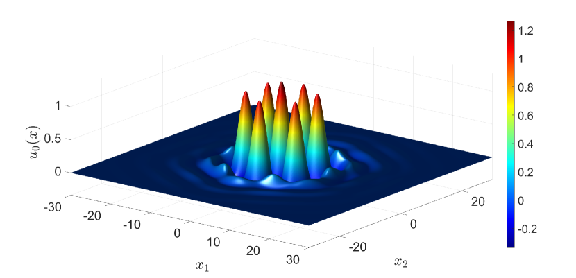
Figure 3: Hexagonal pattern

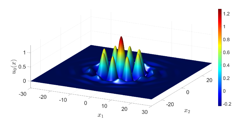
Figure 4: Octogonal pattern

Numerically we obtained three candidates that we denote $u_{s},u_{h}$ and $u_{o}$ informatively as they correspond to “square”, “hexagonal” and “octagonal” symmetries respectively (see Figures 2, 3 and 4). Each candidate is represented through a Fourier series using the construction of Section 3.1. For each case, we perform a computer-assisted proof based on Theorem 3.1. The bounds $\mathcal{Y}_{0},\mathcal{Z}_{1}$ and $\mathcal{Z}_{2}$ are computed numerically using the code available at [1]. More specifically, we choose $N_{0}=130$, $N=90$ for the computations of Section 3.4 and we compute matrix norms of size $91^{2}=8281.$ For each case, we verify rigorously that the condition (34) of Theorem 3.1 is satisfied for some $r_{0}>0.$ This implies the existence of a unique solution of (3) in $\overline{B_{r_{0}}(u_{k})}$ where $k\in\{s,h,o\}$.

Moreover, by proving the existence of a localized pattern, we prove simultaneously the existence of a branch of periodic solutions using Theorem 3.7. In particular, the branch limits the localized pattern as the period tends to infinity. This result has been conjectured in [24] in the context of the 1D quintic SH equation as the authors observed a continuum of periodic solutions, parameterized by the period, that limits to a localized pattern as the period goes to infinity.

For each computer-assisted proof, we provide the parameters at which the proof is obtained as well as the radius of contraction $r_{0}$ (cf. Theorem 3.1). We expose the results in the three Theorems 4.1, 4.2 and 4.3 below. In particular, all computational aspects are implemented in Julia (cf. [53]) via the package RadiiPolynomial.jl (cf. [54]) which relies on the package IntervalArithmetic.jl (cf. [48]) for rigorous interval arithmetic computations. The specific algorithmic details complementing this article can be found at [1].

Theorem 4.1 (The square pattern).

Let $\mu=0.27$, $\nu_{1}=-1.6$ and $\nu_{2}=1$. Let $r_{0}\stackrel{{\scriptstyle\mbox{\tiny{\raisebox{0.0pt}[0.0pt][0.0pt]{def}}}}}{{=}}1.16\times 10^{-5}$, then there exists a unique solution $\tilde{u}$ to (3) in $\overline{B_{r_{0}}(u_{s})}\subset H^{l}_{D_{2}}$ and we have that $\|\tilde{u}-u_{s}\|_{l}\leq r_{0}$. In addition, there exists a smooth curve

$$\left\{\tilde{u}(q):q\in[d,\infty]\right\}\subset C^{\infty}({\mathbb{R}}^{2})$$

such that $\tilde{u}(q)$ is a periodic solution to (3) with period $2q$ in both directions. In particular, $\tilde{u}(\infty)=\tilde{u}$ is a localized pattern on ${\mathbb{R}}^{2}.$

Proof.

Following the notations of Section 3, let us fix $N=90$, $N_{0}=130$ and $d=70$. Then, we construct $u_{0}=\gamma^{\dagger}(U_{0})$ as in (29) and define $u_{s}\stackrel{{\scriptstyle\mbox{\tiny{\raisebox{0.0pt}[0.0pt][0.0pt]{def}}}}}{{=}}u_{0}$, where the construction process is detailed in Section 3.1. Once $U_{0}$ is fixed, we construct $B^{N}$ using the approach described in Section 3.3. In particular, we prove that

$$\|B^{N}\|_{2}\leq 31.6,$$ (105)

which implies that $\|\mathbb{A}\|_{2,l}\leq 31.6$ using (37). Using Lemma 3.8, we start by proving that

$$\kappa\stackrel{{\scriptstyle\mbox{\tiny{\raisebox{0.0pt}[0.0pt][0.0pt]{def}}}}}{{=}}5.62$$

satisfies (96). This allows us to compute the upper bounds introduced in Section 3.4. In particular, using [1], we define

$$\mathcal{Y}_{0}\stackrel{{\scriptstyle\mbox{\tiny{\raisebox{0.0pt}[0.0pt][0.0pt]{def}}}}}{{=}}9.58\times 10^{-6},\leavevmode\nobreak\ \leavevmode\nobreak\ Z_{1}\stackrel{{\scriptstyle\mbox{\tiny{\raisebox{0.0pt}[0.0pt][0.0pt]{def}}}}}{{=}}0.027\leavevmode\nobreak\ \leavevmode\nobreak\ \text{ and }\leavevmode\nobreak\ \leavevmode\nobreak\ \widehat{\mathcal{Z}}_{2}(r)\stackrel{{\scriptstyle\mbox{\tiny{\raisebox{0.0pt}[0.0pt][0.0pt]{def}}}}}{{=}}2988r+315.85$$

for all $r>0$ and prove that ${\mathcal{Y}}_{0}$, $Z_{1}$ and $\widehat{\mathcal{Z}}_{2}$ satisfy (39), (51) and (98) respectively. Then, using the approach presented in Section 3.5.1, we prove that (53) is satisfied for $C_{0}\stackrel{{\scriptstyle\mbox{\tiny{\raisebox{0.0pt}[0.0pt][0.0pt]{def}}}}}{{=}}2.6$. In particular, define $\mathcal{Z}_{u,1}\stackrel{{\scriptstyle\mbox{\tiny{\raisebox{0.0pt}[0.0pt][0.0pt]{def}}}}}{{=}}1.5852\times 10^{-3}$ and $\mathcal{Z}_{u,2}\stackrel{{\scriptstyle\mbox{\tiny{\raisebox{0.0pt}[0.0pt][0.0pt]{def}}}}}{{=}}1.5867\times 10^{-3}$, then we prove that (65) is satisfied and $\mathcal{Z}_{u}\leavevmode\nobreak\ \stackrel{{\scriptstyle\mbox{\tiny{\raisebox{0.0pt}[0.0pt][0.0pt]{def}}}}}{{=}}\leavevmode\nobreak\ \left(\left(\mathcal{Z}_{u,1}\right)+\left(\mathcal{Z}_{u,2}\right)^{2}\right)^{\frac{1}{2}}$ satisfies (44). Consequently, defining $\widehat{\mathcal{Z}}_{1}$ as

$$\widehat{\mathcal{Z}}_{1}\stackrel{{\scriptstyle\mbox{\tiny{\raisebox{0.0pt}[0.0pt][0.0pt]{def}}}}}{{=}}0.17,$$

we obtain that (97) is satisfied. Finally, we prove that $r_{0}=1.16\times 10^{-5}$ satisfies (99). We conclude the proof using Theorem 3.7. ∎

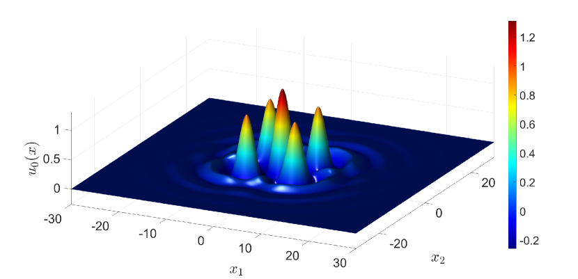
Figure 2: Square pattern

Theorem 4.2 (The hexagonal pattern).

Let $\mu=0.32$, $\nu_{1}=-1.6$ and $\nu_{2}=1$. Let $r_{0}\stackrel{{\scriptstyle\mbox{\tiny{\raisebox{0.0pt}[0.0pt][0.0pt]{def}}}}}{{=}}8.21\times 10^{-6}$, then there exists a unique solution $\tilde{u}$ to (3) in $\overline{B_{r_{0}}(u_{h})}\subset H^{l}_{D_{2}}$ with $\|\tilde{u}-u_{h}\|_{l}\leq r_{0}$. In addition, there exists a smooth curve

$$\left\{\tilde{u}(q):q\in[d,\infty]\right\}\subset C^{\infty}({\mathbb{R}}^{2})$$

such that $\tilde{u}(q)$ is a periodic solution to (3) with period $2q$ in both directions. In particular, $\tilde{u}(\infty)=\tilde{u}$ is a localized pattern on ${\mathbb{R}}^{2}.$

Proof.

The proof is obtained similarly as the one of Theorem 4.1. In particular, we define

$$\kappa \stackrel{{\scriptstyle\mbox{\tiny{\raisebox{0.0pt}[0.0pt][0.0pt]{def}}}}}{{=}}4.86$$

$$\mathcal{Y}_{0}\stackrel{{\scriptstyle\mbox{\tiny{\raisebox{0.0pt}[0.0pt][0.0pt]{def}}}}}{{=}}7.57\times 10^{-6},\leavevmode\nobreak\ \leavevmode\nobreak\ \widehat{\mathcal{Z}}_{1} \stackrel{{\scriptstyle\mbox{\tiny{\raisebox{0.0pt}[0.0pt][0.0pt]{def}}}}}{{=}}0.078\leavevmode\nobreak\ \leavevmode\nobreak\ \text{ and }\leavevmode\nobreak\ \leavevmode\nobreak\ \widehat{\mathcal{Z}}_{2}(r)\stackrel{{\scriptstyle\mbox{\tiny{\raisebox{0.0pt}[0.0pt][0.0pt]{def}}}}}{{=}}1464r+197.8$$

for all $r>0$ and prove that $\kappa,{\mathcal{Y}}_{0}$, $\widehat{\mathcal{Z}}_{1}$ and $\widehat{\mathcal{Z}}_{2}$ satisfy (96), (39), (97) and (98) respectively. ∎

Theorem 4.3 (The octogonal pattern).

Let $\mu=0.27$, $\nu_{1}=-1.6$ and $\nu_{2}=1$. Let $r_{0}\stackrel{{\scriptstyle\mbox{\tiny{\raisebox{0.0pt}[0.0pt][0.0pt]{def}}}}}{{=}}3.86\times 10^{-5}$, then there exists a unique solution $\tilde{u}$ to (3) in $\overline{B_{r_{0}}(u_{o})}\subset H^{l}_{D_{2}}$ with $\|\tilde{u}-u_{o}\|_{l}\leq r_{0}$. In addition, there exists a smooth curve

$$\left\{\tilde{u}(q):q\in[d,\infty]\right\}\subset C^{\infty}({\mathbb{R}}^{2})$$

such that $\tilde{u}(q)$ is a periodic solution to (3) with period $2q$ in both directions. In particular, $\tilde{u}(\infty)=\tilde{u}$ is a localized pattern on ${\mathbb{R}}^{2}.$

Proof.

The proof is obtained similarly as the one of Theorem 4.1. In particular, we define

$$\kappa \stackrel{{\scriptstyle\mbox{\tiny{\raisebox{0.0pt}[0.0pt][0.0pt]{def}}}}}{{=}}5.43$$

$$\mathcal{Y}_{0}\stackrel{{\scriptstyle\mbox{\tiny{\raisebox{0.0pt}[0.0pt][0.0pt]{def}}}}}{{=}}2.7\times 10^{-5},\leavevmode\nobreak\ \leavevmode\nobreak\ \widehat{\mathcal{Z}}_{1} \stackrel{{\scriptstyle\mbox{\tiny{\raisebox{0.0pt}[0.0pt][0.0pt]{def}}}}}{{=}}0.286\leavevmode\nobreak\ \leavevmode\nobreak\ \text{ and }\leavevmode\nobreak\ \leavevmode\nobreak\ \widehat{\mathcal{Z}}_{2}(r)\stackrel{{\scriptstyle\mbox{\tiny{\raisebox{0.0pt}[0.0pt][0.0pt]{def}}}}}{{=}}10402r+907.8$$

for all $r>0$ and prove that $\kappa,{\mathcal{Y}}_{0}$, $\widehat{\mathcal{Z}}_{1}$ and $\widehat{\mathcal{Z}}_{2}$ satisfy (96), (39), (97) and (98) respectively. ∎

5 Acknowledgments

The authors wish to thank Prof. Jason Bramburger from Concordia University for his insights and fruitful discussions. JPL and JCN would like to acknowledge partial funding from the NSERC Discovery grant program.

6 Appendix : Proof of Proposition 3.2

We expose in the Appendix the proof of Proposition 3.2. First, we present a preliminary result which will be useful for our computations.

Lemma 6.1.

Let $n_{1}\geq 0$ and $x_{1},z_{1}\in(-d,d)$, then

$$\int_{-d}^{d}e^{-a|y_{1}-x_{1}|}e^{-a|y_{1}-z_{1}-2dn_{1}|}dy_{1}$$

$$= \begin{cases}(d-x_{1}+\frac{1}{2a})e^{-a(2dn_{1}+z_{1}-x_{1})}-\frac{e^{-a(2d(n_{1}+1)+z_{1}+x_{1})}}{2a}&\text{ if }n_{1}>0\\ (|z_{1}-x_{1}|+\frac{1}{a})e^{-a|z_{1}-x_{1}|}-\frac{e^{-2ad}}{2a}(e^{-a(x_{1}+z_{1})}+e^{a(x_{1}+z_{1})})\leavevmode\nobreak\ &\text{ if }n_{1}=0.\end{cases}$$ (106)

Similarly,

$$\int_{2dn_{1}-d}^{2dn_{1}+d}e^{-a|y_{1}-x_{1}|}e^{-a|y_{1}-z_{1}-2dn_{1}|}dy_{1}$$

$$= \begin{cases}(d+z_{1}+\frac{1}{2a})e^{-a(2dn_{1}+z_{1}-x_{1})}-\frac{e^{-a(2d(n_{1}+1)-z_{1}-x_{1}))}}{2a}&\text{ if }n_{1}>0\\ (|z_{1}-x_{1}|+\frac{1}{a})e^{-a|z_{1}-x_{1}|}-\frac{e^{-2ad}}{2a}(e^{-a(x_{1}+z_{1})}+e^{a(x_{1}+z_{1})})\leavevmode\nobreak\ &\text{ if }n_{1}=0.\end{cases}$$ (107)

Finally, for all $\alpha,\beta\in\mathbb{R}$, we have that

$$\int_{\mathbb{R}}e^{-a|y_{1}-\alpha|}e^{-a|y_{1}-\beta|}dy_{1}=(|\alpha-\beta|+\frac{1}{a})e^{-a|\alpha-\beta|}.$$ (108)

Proof.

Let us first prove (6.1). Suppose first that $n_{1}>0$, then

$$\int_{-d}^{d}e^{-a|y_{1}-x_{1}|}e^{-a|y_{1}-z_{1}-2dn_{1}|}dy_{1}=\int_{-d}^{d}e^{-a|y_{1}-x_{1}|}e^{-a(2dn_{1}+z_{1}-y_{1})}dy_{1}$$

as $2dn_{1}>y_{1}-z_{1}$ for all $y_{1}\in(-d,d)$ as $z_{1}\in(-d,d).$ Therefore, we get

$$\int_{-d}^{d}e^{-a|y_{1}-x_{1}|}e^{-a|y_{1}-z_{1}-2dn_{1}|}dy_{1} =\int_{-d}^{x_{1}}e^{-a(x_{1}-y_{1})}e^{-a(2dn_{1}+z_{1}-y_{1})}dy_{1}$$

$$\quad+\int_{x_{1}}^{d}e^{-a(y_{1}-x_{1})}e^{-a(2dn_{1}+z_{1}-y_{1})}dy_{1}$$

$$=\frac{1}{2a}e^{-a(2dn_{1}+z_{1}+x_{1})}\left(e^{2ax_{1}}-e^{-2ad}\right)+(d-x_{1})e^{-a(2dn_{1}+z_{1}-x_{1})}$$

$$=e^{-a(2dn_{1}+z_{1}-x_{1})}\left(d-x_{1}+\frac{1}{2a}\right)-\frac{e^{-a(2d(n_{1}+1)+z_{1}+x_{1})}}{2a}.$$ (109)

Now if $n_{1}=0$, we first suppose that $z_{1}\geq x_{1}$, then

$$\int_{-d}^{d}e^{-a|y_{1}-x_{1}|}e^{-a|y_{1}-z_{1}-2dn_{1}|}dy_{1}$$

$$= \leavevmode\nobreak\ \int_{-d}^{x_{1}}e^{-a(x_{1}-y_{1})}e^{-a(z_{1}-y_{1})}dy_{1}+\int_{x_{1}}^{z_{1}}e^{-a(y_{1}-x_{1})}e^{-a(z_{1}-y_{1})}dy_{1}+\int_{z_{1}}^{d}e^{-a(y_{1}-x_{1})}e^{-a(y_{1}-z_{1})}dy_{1}$$

$$= \leavevmode\nobreak\ \frac{e^{-a(z_{1}+x_{1})}}{2a}\left(e^{2ax_{1}}-e^{-2ad}\right)+(z_{1}-x_{1})e^{-a(z_{1}-x_{1})}+\frac{e^{a(z_{1}+x_{1})}}{2a}\left(e^{-2az_{1}}-e^{-2ad}\right)$$

$$= \leavevmode\nobreak\ e^{-a(z_{1}-x_{1})}\left(z_{1}-x_{1}+\frac{1}{a}\right)+\frac{e^{-2ad}}{2a}\left(e^{a(z_{1}+x_{1})+e^{-a(z_{1}+x_{1})}}\right).$$ (110)

A similar reasoning can be applied when $x_{1}\geq z_{1}$ and we obtain (6.1).

In order to prove (6.1), notice that

$$\int_{2dn_{1}-d}^{2dn_{1}+d}e^{-a|y_{1}-x_{1}|}e^{-a|y_{1}-z_{1}-2dn_{1}|}dy_{1} =\int_{-d}^{d}e^{-a|y_{1}+2dn_{1}-x_{1}|}e^{-a|y_{1}-z_{1}|}dy_{1}$$

$$=\int_{-d}^{d}e^{-a|-y_{1}+2dn_{1}-x_{1}|}e^{-a|y_{1}+z_{1}|}dy_{1}$$

$$=\int_{-d}^{d}e^{-a|y_{1}+x_{1}-2dn_{1}|}e^{-a|y_{1}+z_{1}|}dy_{1}$$

where we used the changes of variable $y_{1}\mapsto y_{1}+2dn_{1}$ and $y_{1}\mapsto-y_{1}$. In particular, the previous computations in (6) can be used where $x_{1}$ becomes $-z_{1}$ and $z_{1}$ becomes $-x_{1}$. This proves (6.1).

Finally, to prove (108), we use (6) and take the limit as $d\to\infty$. This concludes the proof. ∎

Now let $u\in L^{2}_{D_{2}}$ such that $\|u\|_{2}=1$ and define $v\stackrel{{\scriptstyle\mbox{\tiny{\raisebox{0.0pt}[0.0pt][0.0pt]{def}}}}}{{=}}v_{0}^{N}u$ where $v_{0}^{N}$ is defined in (43). Then, recalling (64), we need to verify that the constants $C_{1}(d),C_{12}(d)$ and $C_{2}(d)>0$ given in (63) satisfy

$$\sum_{n\in\mathbb{N}_{0}^{2},n\neq 0}\alpha_{n}\int_{\mathbb{R}^{2}\setminus({\Omega_{0}}\cup({\Omega_{0}}+2dn))}\int_{\Omega_{0}}\int_{\Omega_{0}}e^{-a|y-x|_{1}}e^{-a|y-2dn-z|_{1}}|v(x)v(z)|dxdzdy$$ (111)

$$\leq \leavevmode\nobreak\ e^{-4ad}|{\Omega_{0}}|\left(V_{0}^{N},V_{0}^{N}*\left[C_{1}(d)E_{1}+C_{12}(d)E_{1,2}+C_{2}(d)E_{2}\right]\right)_{2},$$

where ${E_{1}},{E_{1,2}}$ and ${E_{2}}$ are sequences in $\ell^{2}_{D_{2}}$ defined in (62). Using Fubini’s theorem on the left-hand side of (111), our goal is to compute an upper bound for

$$\int_{{\Omega_{0}}}\int_{{\Omega_{0}}}|v(x)v(z)|\left(\int_{\mathbb{R}^{2}\setminus({\Omega_{0}}\cup({\Omega_{0}}+2dn))}e^{-a|y-x|_{1}}e^{-a|y-2dn-z|_{1}}dy\right)dzdx$$

for the cases $n_{1},n_{2}>0$ (Section 6.1), $n_{1}>0,n_{2}=0$ (Section 6.2) and $n_{1}=0,n_{2}>0$ (Section 6.3). Before presenting our analysis for each case, we first introduce some notations. Let $n\in\mathbb{N}_{0}^{2}$, $x,z\in\Omega_{0}$, and denote

$$I^{1}_{n}(x_{1},z_{1}) \stackrel{{\scriptstyle\mbox{\tiny{\raisebox{0.0pt}[0.0pt][0.0pt]{def}}}}}{{=}}\int_{\mathbb{R}}e^{-a|y_{1}-x_{1}|}e^{-a|y_{1}-z_{1}-2dn_{1}|}dy_{1}$$ (112)

$$I^{2}_{n}(x_{1},z_{1}) \stackrel{{\scriptstyle\mbox{\tiny{\raisebox{0.0pt}[0.0pt][0.0pt]{def}}}}}{{=}}\int_{-d}^{d}e^{-a|y_{1}-x_{1}|}e^{-a|y_{1}-z_{1}-2dn_{1}|}dy_{1}$$

$$I^{3}_{n}(x_{1},z_{1}) \stackrel{{\scriptstyle\mbox{\tiny{\raisebox{0.0pt}[0.0pt][0.0pt]{def}}}}}{{=}}\int_{2dn_{1}-d}^{2dn_{1}+d}e^{-a|y_{1}-x_{1}|}e^{-a|y_{1}-z_{1}-2dn_{1}|}dy_{1}$$

$$J^{1}_{n}(x_{2},z_{2}) \stackrel{{\scriptstyle\mbox{\tiny{\raisebox{0.0pt}[0.0pt][0.0pt]{def}}}}}{{=}}\int_{\mathbb{R}}e^{-a|y_{2}-x_{2}|}e^{-a|y_{2}-z_{2}-2dn_{2}|}dy_{2}$$

$$J^{2}_{n}(x_{2},z_{2}) \stackrel{{\scriptstyle\mbox{\tiny{\raisebox{0.0pt}[0.0pt][0.0pt]{def}}}}}{{=}}\int_{-d}^{d}e^{-a|y_{2}-x_{2}|}e^{-a|y_{2}-z_{2}-2dn_{2}|}dy_{2}$$

$$J^{3}_{n}(x_{2},z_{2}) \stackrel{{\scriptstyle\mbox{\tiny{\raisebox{0.0pt}[0.0pt][0.0pt]{def}}}}}{{=}}\int_{2dn_{2}-d}^{2dn_{2}+d}e^{-a|y_{2}-x_{2}|}e^{-a|y_{2}-z_{2}-2dn_{2}|}dy_{2}.$$

To simplify notations, we will drop the dependency in $x$ and $z$ when no confusion arises. Moreover, we introduce three sequences $(p_{n})_{n\in\mathbb{N}_{0}^{2}},(q_{n})_{n\in\mathbb{N}_{0}^{2}}$ and $(s_{n})_{n\in\mathbb{N}_{0}^{2}}$ defined as

$$p_{n} \stackrel{{\scriptstyle\mbox{\tiny{\raisebox{0.0pt}[0.0pt][0.0pt]{def}}}}}{{=}}\begin{cases}4e^{-2ad(n_{1}+n_{2}-1)}\left(2d(n_{2}-1)+\frac{1}{a}\right)\left(2d(n_{1}-1)+\frac{e^{-2ad}}{a}\right)&\text{ if }n_{1},n_{2}>0\\ \frac{2e^{-2adn_{1}}}{a}\left(2d(n_{1}-1)+\frac{e^{-2ad}}{a}\right)&\text{ if }n_{1}>0,n_{2}=0\\ 0&\text{ otherwise}\end{cases}$$ (113)

$$q_{n} \stackrel{{\scriptstyle\mbox{\tiny{\raisebox{0.0pt}[0.0pt][0.0pt]{def}}}}}{{=}}\begin{cases}8e^{-2ad(n_{1}+n_{2})}\left(2n_{2}d+\frac{1+e^{-2ad}}{2a}\right)\left(2d+\frac{1}{2a}\right)&\text{ if }n_{1},n_{2}>0\\ \frac{4e^{-2ad(n_{1}+1)}}{a}\left(2d+\frac{1}{a}\right)&\text{ if }n_{1}>0,n_{2}=0\\ q_{n}=\frac{4e^{-2ad(n_{2}+1)}}{a}\left(2d+\frac{1}{a}\right)&\text{ if }n_{1}=0,n_{2}>0\\ 0&\text{ if }n_{1}=n_{2}=0\end{cases}$$

$$s_{n} \stackrel{{\scriptstyle\mbox{\tiny{\raisebox{0.0pt}[0.0pt][0.0pt]{def}}}}}{{=}}\begin{cases}\frac{2e^{-2adn_{2}}}{a}\left(2d(n_{2}-1)+\frac{e^{-2ad}}{a}\right)&\text{ if }n_{1}=0,n_{2}>0\\ 0&\text{ otherwise}.\end{cases}$$

6.1 Case $n_{1},n_{2}>0$

Let $n_{1},n_{2}>0$, then using (112), we get

$$\displaystyle\int_{\mathbb{R}^{2}\setminus({\Omega_{0}}\cup({\Omega_{0}}+2dn))}e^{-a|y-x|_{1}}e^{-a|y-z-2dn|_{1}}dy =I^{1}_{n}J^{1}_{n}-I^{2}_{n}J^{2}_{n}-I^{3}_{n}J^{3}_{n}$$

$$=(I^{1}_{n}-I^{2}_{n}-I^{3}_{n})J^{1}_{n}+(J^{1}_{n}-J^{2}_{n})I^{2}_{n}+(J^{1}_{n}-J^{3}_{n})I^{3}_{n}.$$

Then, using Lemma 6.1, we obtain

$$I_{n}^{1}=\left(2dn_{1}+z_{1}-x_{1}+\frac{1}{a}\right)e^{-a(2dn_{1}+z_{1}-x_{1})}\text{ and }J_{n}^{1}=\left(2dn_{2}+z_{2}-x_{2}+\frac{1}{a}\right)e^{-a(2dn_{2}+z_{2}-x_{2})}$$ (114)

as $2dn_{1}\geq x_{1}-z_{1}$ and $2dn_{2}\geq x_{2}-z_{2}$. Given a fixed $\alpha\geq 0$, let $h:\mathbb{R}^{+}\to\mathbb{R}^{+}$ be defined as

$$h(r)=\left(\alpha+r+\frac{1}{a}\right)e^{-a(\alpha+r)}.$$

Then

$$h^{\prime}(r)=e^{-a(\alpha+r)}\left(1-a(\alpha+r+\frac{1}{a})\right)=-ae^{-a(\alpha+r)}(\alpha+r)\leq 0$$

for all $r\geq 0.$ In particular, $h$ has a global minimum at $r=0$. Denoting $r=2d+z_{2}-x_{2}$ and $\alpha=2d(n_{2}-1)$, we obtain that

$$J_{n}^{1}=h(r)\leq h(0)=\left(2d(n_{2}-1)+\frac{1}{a}\right)e^{-2ad(n_{2}-1)}.$$ (115)

Therefore, using Lemma 6.1 and (115) we get

$$I^{1}_{n}-I^{2}_{n}-I^{3}_{n} =2d(n_{1}-1)e^{-a(2dn_{1}+z_{1}-x_{1})}+\frac{e^{-2ad(n_{1}+1)}}{2a}\left(e^{a(x_{1}+z_{1})}+e^{-a(x_{1}+z_{1})}\right)$$

$$J^{1}_{n} \leq\left(2d(n_{2}-1)+\frac{1}{a}\right)e^{-2da(n_{2}-1)}$$

$$J^{1}_{n}-J^{2}_{n} =\left(d(2n_{2}-1)+z_{2}+\frac{1}{2a}\right)e^{-a(2dn_{2}+z_{2}-x_{2})}+\frac{e^{-a(2d(n_{2}+1)+z_{2}+x_{2})}}{2a}$$

$$J^{1}_{n}-J^{3}_{n} =\left(d(2n_{2}-1)-x_{2}+\frac{1}{2a}\right)e^{-a(2dn_{2}+z_{2}-x_{2})}+\frac{e^{-a(2d(n_{2}+1)-z_{2}-x_{2})}}{2a}.$$ (116)

Consequently, we use (6.1) to get

$$\int_{{\Omega_{0}}}\int_{{\Omega_{0}}}v(x)v(z)(I^{1}_{n}-I^{2}_{n}-I^{3}_{n})dxdz\leq \leavevmode\nobreak\ 2d(n_{1}-1)e^{-2adn_{1}}\int_{{\Omega_{0}}}v(x)e^{ax_{1}}dx\int_{{\Omega_{0}}}v(z)e^{-az_{1}}dz$$

$$+ \leavevmode\nobreak\ \frac{e^{-2ad(n_{1}+1)}}{2a}\int_{{\Omega_{0}}}\int_{{\Omega_{0}}}v(x)v(z)\left(e^{a(x_{1}+z_{1})}+e^{-a(x_{1}+z_{1})}\right)dxdz$$

But using that $v\in L_{D_{2}}^{2}$, we simplify

$$\int_{{\Omega_{0}}}\int_{{\Omega_{0}}}v(x)v(z)(I^{1}_{n}-I^{2}_{n}-I^{3}_{n})dxdz$$

$$\leq \leavevmode\nobreak\ 2d(n_{1}-1)e^{-2adn_{1}}\left(\int_{{\Omega_{0}}}v(x)e^{ax_{1}}dx\right)^{2}+\frac{e^{-2ad(n_{1}+1)}}{a}\left(\int_{{\Omega_{0}}}v(x)e^{ax_{1}}dx\right)^{2},$$

which implies that

$$\int_{{\Omega_{0}}}\int_{{\Omega_{0}}}v(x)v(z)(I^{1}_{n}-I^{2}_{n}-I^{3}_{n})dxdz\leq\left({2d(n_{1}-1)e^{-2adn_{1}}}+\frac{e^{-2ad(n_{1}+1)}}{a}\right)\left(\int_{{\Omega_{0}}}v(x)e^{ax_{1}}dx\right)^{2}.$$ (117)

Now, using Cauchy-Schwartz inequality, we obtain

$$\left(\int_{{\Omega_{0}}}v(x)e^{ax_{1}}dx\right)^{2}\leq\int_{{\Omega_{0}}}|u(x)|^{2}dx\int_{{\Omega_{0}}}v_{0}^{N}(x)^{2}e^{2ax_{1}}dx\leq\int_{{\Omega_{0}}}v_{0}^{N}(x)^{2}e^{2ax_{1}}dx$$ (118)

using that $v=v_{0}^{N}u$ by definition and $\|u\|_{2}=1$. Moreover, as $v_{0}^{N}$ is $D_{2}$-symmetric, we have

$$\int_{{\Omega_{0}}}v_{0}^{N}(x)^{2}e^{2ax_{1}}dx=\int_{{\Omega_{0}}}v_{0}^{N}(x)^{2}\cosh(2ax_{1})dx=|{\Omega_{0}}|(V^{N}_{0},V^{N}_{0}*E_{1})_{2},$$ (119)

where we used Parseval’s identity for the last step. Therefore, combining (115), (117) and (118), we get

$$\int_{{\Omega_{0}}}\int_{{\Omega_{0}}}v(x)v(z)(I^{1}_{n}-I^{2}_{n}-I^{3}_{n})J^{1}_{n}dxdz\leq\frac{p_{n}}{4}|{\Omega_{0}}|(V^{N}_{0},V^{N}_{0}*E_{1})_{2}$$ (120)

where $p_{n}$ is defined in (113). Now, notice that $I^{2}_{n}\leq\left(d-x_{1}+\frac{1}{2a}\right)e^{-a(2dn_{1}+z_{1}-x_{1})}$, then using (6.1) and $|z_{2}|,|x_{1}|\leq d$ for all $z_{2},x_{1}\in(-d,d)$, we get

$$\int_{{\Omega_{0}}}\int_{{\Omega_{0}}}v(x)v(z)(J^{1}_{n}-J^{2}_{n})I^{2}_{n}dxdz$$

$$\leq \leavevmode\nobreak\ \int_{{\Omega_{0}}}\int_{{\Omega_{0}}}v(z)v(x)\left(2n_{2}d+\frac{1}{2a}\right)e^{-a(2dn_{2}+z_{2}-x_{2})}\left(2d+\frac{1}{2a}\right)e^{-a(2dn_{1}+z_{1}-x_{1})}dxdz$$

$$+\int_{{\Omega_{0}}}\int_{{\Omega_{0}}}v(z)v(x)\frac{e^{-a(2d(n_{2}+1)+z_{2}+x_{2})}}{2a}\left(2d+\frac{1}{2a}\right)e^{-a(2dn_{1}+z_{1}-x_{1})}dxdz$$

$$= \leavevmode\nobreak\ \left(2n_{2}d+\frac{1}{2a}\right)\left(2d+\frac{1}{2a}\right)e^{-2ad(n_{1}+n_{2})}\int_{{\Omega_{0}}}v(z)e^{-a(z_{2}+z_{1})}dz\int_{{\Omega_{0}}}v(x)e^{a(x_{2}+x_{1})}dx$$

$$+\left(2d+\frac{1}{2a}\right)\frac{e^{-2ad(n_{1}+n_{2}+1)}}{2a}\int_{{\Omega_{0}}}v(z)e^{-a(z_{2}+z_{1})}dz\int_{{\Omega_{0}}}v(x)e^{a(x_{1}-x_{2})}dx.$$ (121)

Using again that $v\in L^{2}_{D_{2}}$ and Cauchy-Schwartz inequality, we obtain

$$\int_{{\Omega_{0}}}\int_{{\Omega_{0}}}v(x)v(z)(J^{1}_{n}-J^{2}_{n})I^{2}_{n}dxdz$$

$$\leq\leavevmode\nobreak\ e^{-2ad(n_{1}+n_{2})}\left[\left(2n_{2}d+\frac{1}{2a}\right)\left(2d+\frac{1}{2a}\right)+\frac{e^{-2ad}}{2a}\left(2d+\frac{1}{2a}\right)\right]\left(\int_{{\Omega_{0}}}v(z)e^{a(z_{2}+z_{1})}dz\right)^{2}$$

$$\leq\leavevmode\nobreak\ e^{-2ad(n_{1}+n_{2})}\left(2n_{2}d+\frac{1+e^{-2ad}}{2a}\right)\left(2d+\frac{1}{2a}\right)\left(\int_{{\Omega_{0}}}v(z)e^{a(z_{2}+z_{1})}dz\right)^{2}$$

$$\leq\leavevmode\nobreak\ e^{-2ad(n_{1}+n_{2})}\left(2n_{2}d+\frac{1+e^{-2ad}}{2a}\right)\left(2d+\frac{1}{2a}\right)\int_{{\Omega_{0}}}v_{0}^{N}(z)^{2}e^{2a(z_{2}+z_{1})}dz.$$ (122)

Moreover, as in (119), we have

$$\int_{{\Omega_{0}}}v_{0}^{N}(z)^{2}e^{2a(z_{2}+z_{1})}dz=\int_{{\Omega_{0}}}v_{0}^{N}(z)^{2}\cosh(2az_{1})\cosh(2az_{2})dz=|{\Omega_{0}}|(V^{N}_{0},V^{N}_{0}*E_{1,2})_{2}.$$

Therefore we obtain

$$\int_{{\Omega_{0}}}\int_{{\Omega_{0}}}v(x)v(z)(J^{1}_{n}-J^{2}_{n})I^{2}_{n}dxdz\leq\frac{q_{n}}{8}|{\Omega_{0}}|(V^{N}_{0},V^{N}_{0}*E_{1,2})_{2}$$ (123)

where $q_{n}$ is defined in (113). Similarly, using (6.1) we get

$$\int_{{\Omega_{0}}}\int_{{\Omega_{0}}}v(x)v(z)(J^{1}_{n}-J^{3}_{n})I^{3}_{n}dxdz\leq\frac{q_{n}}{8}|{\Omega_{0}}|(V^{N}_{0},V^{N}_{0}*E_{1,2})_{2}$$

using (123). Summarizing the results of the section, for all $n_{1},n_{2}>0$ we have that

$$\int_{{\Omega_{0}}}\int_{{\Omega_{0}}}|v(x)v(z)|\left(\int_{\mathbb{R}^{2}\setminus({\Omega_{0}}\cup({\Omega_{0}}+2dn))}e^{-a|y-x|_{1}}e^{-a|y-2dn-x|_{1}}dy\right)dzdx$$

$$\qquad\leq\frac{p_{n}}{4}|{\Omega_{0}}|(V^{N}_{0},V^{N}_{0}*E_{1})_{2}+\frac{q_{n}}{4}|{\Omega_{0}}|(V^{N}_{0},V^{N}_{0}*E_{1,2})_{2}.$$

6.2 Case $n_{1}>0,n_{2}=0$

Let $n_{1}>0,n_{2}=0$, then $J^{2}_{n}=J^{3}_{n}$ and

$$\displaystyle\int_{\mathbb{R}^{2}\setminus({\Omega_{0}}\cup({\Omega_{0}}+2dn))}e^{-a|y-x|_{1}}e^{-a|y-z-2dn|_{1}}dy =I^{1}_{n}J^{1}_{n}-I^{2}_{n}J^{2}_{n}-I^{3}_{n}J^{2}_{n}$$

$$=(I^{1}_{n}-I^{2}_{n}-I^{3}_{n})J^{1}_{n}+(J^{1}_{n}-J^{2}_{n})(I^{2}_{n}+I^{3}_{n}).$$ (124)

First, notice that $J^{1}_{n}\leq\frac{1}{a}$, then

$$\int_{{\Omega_{0}}}\int_{{\Omega_{0}}}v(x)v(z)(I^{1}_{n}-I^{2}_{n}-I^{3}_{n})J^{1}_{n}dxdz\leq\frac{1}{a}\int_{{\Omega_{0}}}\int_{{\Omega_{0}}}v(x)v(z)(I^{1}_{n}-I^{2}_{n}-I^{3}_{n})dxdz.$$

Then, using (117) and (118), we get

$$\int_{{\Omega_{0}}}\int_{{\Omega_{0}}}v(x)v(z)(I^{1}_{n}-I^{2}_{n}-I^{3}_{n})J^{1}_{n}dxdz\leq\frac{p_{n}}{2}|{\Omega_{0}}|(V^{N}_{0},V^{N}_{0}*E_{1})_{2}$$ (125)

where $p_{n}$ is defined in (113). Then, we use Lemma 6.1 to get

$$J^{1}_{n}-J^{2}_{n}=\frac{e^{-2ad}}{2a}\left(e^{-a(x_{2}+z_{2})}+e^{a(x_{2}+z_{2})}\right)$$ (126)

and

$$I_{n}^{2}\leq(d-x_{1}+\frac{1}{2a})e^{-a(2dn_{1}+z_{1}-x_{1})}\text{ and }I_{n}^{3}\leq(d+z_{1}+\frac{1}{2a})e^{-a(2dn_{1}+z_{1}-x_{1})}.$$ (127)

Using (126) and (127), we get

$$\int_{{\Omega_{0}}}\int_{{\Omega_{0}}}v(x)v(z)(J^{1}_{n}-J^{2}_{n})(I^{2}_{n}+I^{3}_{n})dxdz$$

$$\leq \frac{e^{-2ad(n_{1}+1)}}{2a}\int_{{\Omega_{0}}}\int_{{\Omega_{0}}}v(x)v(z)\left(e^{-a(x_{2}+z_{2})}+e^{a(x_{2}+z_{2})}\right)(d+z_{1}+\frac{1}{2a})e^{-a(z_{1}-x_{1})}$$

$$+\frac{e^{-2ad(n_{1}+1)}}{2a}\int_{{\Omega_{0}}}\int_{{\Omega_{0}}}v(x)v(z)\left(e^{-a(x_{2}+z_{2})}+e^{a(x_{2}+z_{2})}\right)(d-x_{1}+\frac{1}{2a})e^{-a(z_{1}-x_{1})}.$$

Therefore, similarly as in (6.1) and (6.1), we use that $v\in L^{2}_{D_{2}}$ and the Cauchy-Schwartz inequality to obtain

$$\int_{{\Omega_{0}}}\int_{{\Omega_{0}}}v(x)v(z)(J^{1}_{n}-J^{2}_{n})(I^{2}_{n}+I^{3}_{n})dxdz\leq\frac{q_{n}}{2}|{\Omega_{0}}|(V^{N}_{0},V^{N}_{0}*E_{1,2})_{2}$$

where $q_{n}$ is given in (113).

6.3 Case $n_{1}=0,n_{2}>0$

Similarly, as in Section 6.2, we have

$$\displaystyle\int_{\mathbb{R}^{2}\setminus({\Omega_{0}}\cup({\Omega_{0}}+2dn))}e^{-a|y-x|_{1}}e^{-a|y-z-2dn|_{1}}dy =I^{1}_{n}J^{1}_{n}-I^{2}_{n}J^{2}_{n}-I^{2}_{n}J^{3}_{n}$$

$$=(J^{1}_{n}-J^{2}_{n}-J^{3}_{n})I^{1}_{n}+(I^{1}_{n}-I^{2}_{n})(J^{2}_{n}+J^{3}_{n}).$$

In fact, the needed computations are identical as the ones of Section 6.2 interchanging the subscripts 1 and 2. In particular, we obtain that

$$\int_{{\Omega_{0}}}\int_{{\Omega_{0}}}v(x)v(z)(J^{1}_{n}-J^{2}_{n}-J^{3}_{n})I^{1}_{n}dxdz\leq\frac{s_{n}}{2}|{\Omega_{0}}|(V^{N}_{0},E_{2}*V^{N}_{0})_{2}$$

where $s_{n}$ is defined in (113). Similarly,

$$\int_{{\Omega_{0}}}\int_{{\Omega_{0}}}v(x)v(z)(I^{1}_{n}-I^{2}_{n})(J^{2}_{n}+J^{3}_{n})dxdz\leq\frac{q_{n}}{2}|{\Omega_{0}}|(V^{N}_{0},V^{N}_{0}*E_{1,2})_{2}.$$

6.4 Summary and computation of $C_{1}(d),C_{12}(d)$ and $C_{2}(d)$

Combining the results from Sections 6.1, 6.2 and 6.3, we get

$$\sum_{n\in\mathbb{N}^{2}_{0},n\neq 0}\alpha_{n}\int_{\mathbb{R}^{2}\setminus({\Omega_{0}}\cup({\Omega_{0}}+2dn))}\mathbb{L}^{-1}v(y)\mathbb{L}^{-1}v(y-2dn)dy$$

$$\leq C_{0}^{2}|{\Omega_{0}}|\left((V_{0}^{N},E_{1}*V^{N}_{0})_{2}\sum_{n\in\mathbb{N}^{2}_{0}}p_{n}+(V_{0}^{N},E_{1,2}*V^{N}_{0})_{2}\sum_{n\in\mathbb{N}^{2}_{0}}q_{n}+(V_{0}^{N},E_{2}*V^{N}_{0})_{2}\sum_{n\in\mathbb{N}^{2}_{0}}s_{n}\right)$$

where $p_{n},\leavevmode\nobreak\ q_{n}$ and $s_{n}$ are defined in (113). Consequently, it remains to compute upper bounds for $\sum_{n\in\mathbb{N}^{2}_{0}}p_{n}$, $\sum_{n\in\mathbb{N}^{2}_{0}}q_{n}$ and $\sum_{n\in\mathbb{N}^{2}_{0}}s_{n}$. The following lemma provides upper bounds for such quantities. The bounds are explicit and decay in $e^{-4ad}.$ This allows us to define explicitly the constants $C_{1}(d),C_{12}(d)$ and $C_{2}(d)$ satisfying (111).

Lemma 6.2.

Let $C_{1}(d),C_{12}(d),C_{2}(d)>0$ be defined in (63), then

$$\sum_{n\in\mathbb{N}^{2}_{0}}p_{n}\leq C_{1}(d)e^{-4ad},\leavevmode\nobreak\ \leavevmode\nobreak\ \sum_{n\in\mathbb{N}^{2}_{0}}q_{n}\leq C_{12}(d)e^{-4ad},\leavevmode\nobreak\ \leavevmode\nobreak\ \sum_{n\in\mathbb{N}^{2}_{0}}s_{n}\leq C_{2}(d)e^{-4ad}.$$ (128)

Proof.

Recall that

$$p_{n}=4e^{-2ad(n_{1}+n_{2}-1)}\left(2d(n_{2}-1)+\frac{1}{a}\right)\left(2d(n_{1}-1)+\frac{e^{-2ad}}{a}\right)$$

for all $n_{1},n_{2}>0.$ Let us define $\tilde{p}_{n}\stackrel{{\scriptstyle\mbox{\tiny{\raisebox{0.0pt}[0.0pt][0.0pt]{def}}}}}{{=}}e^{-2ad(n_{1}+n_{2}-1)}\left(2d(n_{2}-1)+\frac{1}{a}\right)\left(2d(n_{1}-1)+\frac{e^{-2ad}}{a}\right)$. One can easily prove that

$$xe^{-ax}\leq\frac{e^{-1}}{a}$$

for all $x\geq 0$. Therefore,

$$e^{-ad(n_{2}-1)}(2d(n_{2}-1)+\frac{1}{a})\leq\frac{2e^{-1}+1}{a}$$ (129)

for all $n_{2}\geq 1$. Similarly,

$$e^{-adn_{1}}\left((2d(n_{1}-1)+\frac{1}{a}\right)\leq\frac{2e^{-1}+1}{a}$$ (130)

for all $n_{1}\geq 1$, which implies that

$${\tilde{p}}_{n}\leq\frac{(2e^{-1}+1)^{2}}{a^{2}}e^{-ad(n_{1}+n_{2}-1)}$$ (131)

for all $n_{1},n_{2}\geq 1.$ Therefore,

$$\sum_{n_{1}>0,n_{2}>0}{\tilde{p}}_{n}={\tilde{p}}_{1,1}+{\tilde{p}}_{2,1}+{\tilde{p}}_{3,1}+\sum_{n_{1}=1}^{3}\sum_{n_{2}=2}^{\infty}{\tilde{p}}_{n}+\sum_{n_{1}=4}^{\infty}\sum_{n_{2}=1}^{\infty}{\tilde{p}}_{n}.$$ (132)

We readily have

$${\tilde{p}}_{1,1}+{\tilde{p}}_{2,1}+{\tilde{p}}_{3,1}=\frac{e^{-4ad}}{a}\left(2d+\frac{1+e^{-2ad}}{a}+e^{-2ad}\left(4d+\frac{e^{-2ad}}{a}\right)\right)$$

and

$$\sum_{n_{1}=1}^{2}\sum_{n_{2}=2}^{\infty}{\tilde{p}}_{n}=e^{-4ad}\left(\frac{1+e^{-2ad}}{a}+2d\right)\sum_{n_{2}=1}^{\infty}e^{-2ad(n_{2}-1)}\left(2d(n_{2}-1)+\frac{1}{a}\right).$$

Therefore, using (130), we obtain

$$\sum_{n_{1}=1}^{2}\sum_{n_{2}=2}^{\infty}{\tilde{p}}_{n} =e^{-4ad}\left(\frac{1+e^{-2ad}}{a}+2d\right)\sum_{n_{2}=1}^{\infty}e^{-2ad(n_{2}-1)}\left(2d(n_{2}-1)+\frac{1}{a}\right)$$

$$\leq e^{-4ad}\left(\frac{1+e^{-2ad}}{a}+2d\right)\frac{2e^{-1}+1}{a(1-e^{-ad})}.$$

Similarly, using (129) and (130),

$$\sum_{n_{1}=4}^{\infty}\sum_{n_{2}=1}^{\infty}{\tilde{p}}_{n}\leq\frac{(2e^{-1}+1)^{2}}{a^{2}}\sum_{n_{1}=4}^{\infty}\sum_{n_{2}=1}^{\infty}e^{-ad(n_{1}+n_{2}-1)}=e^{-4ad}\frac{(2e^{-1}+1)^{2}}{a^{2}(1-e^{-ad})^{2}}.$$

Therefore we obtain

$$\sum_{n_{1}>0,n_{2}>0}p_{n}\leq 4P_{1}e^{-4ad}$$

where

$$P_{1}\stackrel{{\scriptstyle\mbox{\tiny{\raisebox{0.0pt}[0.0pt][0.0pt]{def}}}}}{{=}}\frac{2ad+1+e^{-2ad}}{a^{2}}+e^{-2ad}\left(4d+\frac{e^{-2ad}}{a}\right)+\left(\frac{1+e^{-2ad}}{a}+2d\right)\frac{2e^{-1}+1}{a(1-e^{-ad})}+\frac{(2e^{-1}+1)^{2}}{a^{2}(1-e^{-ad})^{2}}.$$ (133)

Now recall that

$$p_{n}=\frac{2e^{-2adn_{1}}}{a}\left(2d(n_{1}-1)+\frac{e^{-2ad}}{a}\right)$$

for all $n_{1}>0,n_{2}=0.$

Therefore, using (129),

$$\sum_{n_{1}=1}^{\infty}p_{n} =p_{1,0}+p_{2,0}+p_{3,0}+\sum_{n_{1}=4}^{\infty}p_{n}$$

$$\leq\frac{2e^{-4ad}}{a}\left(\frac{1+e^{-2ad}}{a}+2d+e^{-2ad}(4d+\frac{e^{-2ad}}{a})+\frac{2e+1}{a}\sum_{n_{1}=4}^{\infty}e^{-ad(n_{1}-4)}\right)$$

$$=\frac{2e^{-4ad}}{a}\left(\frac{1+e^{-2ad}}{a}+2d+e^{-2ad}(4d+\frac{e^{-2ad}}{a})+\frac{2e^{-1}+1}{a(1-e^{-ad})}\right).$$

Finally, we obtain that

$$\sum_{n\in\mathbb{N}^{2}_{0}}p_{n}\leq\left(4P_{1}+P_{2}\right)e^{-4ad}\leq C_{1}(d)e^{-4ad}$$

where

$$P_{2} \stackrel{{\scriptstyle\mbox{\tiny{\raisebox{0.0pt}[0.0pt][0.0pt]{def}}}}}{{=}}\frac{2}{a}\left(\frac{1+e^{-2ad}}{a}+2d+e^{-2ad}(4d+\frac{e^{-2ad}}{a})+\frac{2e^{-1}+1}{a(1-e^{-ad})}\right)$$ (134)

and $P_{1}$ is defined in (133). Now, recall that

$$q_{n} \stackrel{{\scriptstyle\mbox{\tiny{\raisebox{0.0pt}[0.0pt][0.0pt]{def}}}}}{{=}}8e^{-2ad(n_{1}+n_{2})}\left(2n_{2}d+\frac{1+e^{-2ad}}{2a}\right)\left(2d+\frac{1}{2a}\right)$$

for all $n_{1},n_{2}>0$. Using (129), we obtain that

$$q_{n}\leq 8\left(2d+\frac{1}{2a}\right)e^{-ad(2n_{1}+n_{2})}\frac{4e^{-1}+1+e^{-2ad}}{2a}$$

for all $n_{1},n_{2}>0$. Therefore,

$$\sum_{n_{1}>0,n_{2}>0}q_{n} =c_{1,1}+\sum_{n_{1}=2}^{\infty}c_{n_{1},1}+\sum_{n_{1}=1}^{\infty}\sum_{n_{2}=2}^{\infty}q_{n}$$

$$\leq 8\left(2d+\frac{1}{2a}\right)e^{-4ad}\left[2d+\frac{1+e^{-2ad}}{2a}+(2d+\frac{1+e^{-2ad}}{2a})\frac{1}{1-e^{-ad}}+\frac{4e^{-1}+1+e^{-2ad}}{2a(1-e^{-ad})^{2}}\right].$$

This implies that

$$\sum_{n_{1}>0,n_{2}>0}q_{n}\leq 8e^{-4ad}Q_{1}\left(2d+\frac{1}{2a}\right)$$

where

$$Q_{1}\stackrel{{\scriptstyle\mbox{\tiny{\raisebox{0.0pt}[0.0pt][0.0pt]{def}}}}}{{=}}2d+\frac{1+e^{-2ad}}{2a}+(2d+\frac{1+e^{-2ad}}{2a})\frac{1}{1-e^{-ad}}+\frac{4e^{-1}+1+e^{-2ad}}{2a(1-e^{-ad})^{2}}.$$ (135)

Moreover, recall that

$$q_{n}=\frac{4e^{-2ad(n_{1}+1)}}{a}\left(2d+\frac{1}{a}\right)$$

for all $n_{1}>0,n_{2}=0$ and similarly,

$$q_{n}=\frac{4e^{-2ad(n_{2}+1)}}{a}\left(2d+\frac{1}{a}\right)$$

for all $n_{1}=0,n_{2}>0.$ Therefore,

$$\sum_{n_{1}=1}^{\infty}q_{n_{1},0}+\sum_{n_{2}=1}^{\infty}q_{0,n_{2}}\leq Q_{2}e^{-4ad}$$

where

$$Q_{2}\stackrel{{\scriptstyle\mbox{\tiny{\raisebox{0.0pt}[0.0pt][0.0pt]{def}}}}}{{=}}\left(2d+\frac{1}{a}\right)\frac{8}{a(1-e^{-2ad})}.$$ (136)

Finally, we obtain

$$\sum_{n\in\mathbb{N}^{2}_{0}}q_{n}\leq 8Q_{1}\left(2d+\frac{1}{2a}\right)+Q_{2}e^{-4ad}\leq C_{12}(d)e^{-4ad}$$

where $Q_{1},Q_{2}$ are defined in (135) and (136) respectively. To conclude, we recall that

$$s_{n} \stackrel{{\scriptstyle\mbox{\tiny{\raisebox{0.0pt}[0.0pt][0.0pt]{def}}}}}{{=}}\frac{2e^{-2adn_{2}}}{a}\left(2d(n_{2}-1)+\frac{e^{-2ad}}{a}\right)$$

for all $n_{2}>0,n_{1}=0$ and $s_{n}=0$ otherwise. Therefore, using (129),

$$\sum_{n_{2}=1}^{\infty}d_{0,n_{2}} =s_{0,1}+s_{0,2}+s_{0,3}+\sum_{n_{2}=4}^{\infty}s_{0,n_{2}}$$

$$\leq\frac{2e^{-4ad}}{a}\left[\frac{1+e^{-2ad}}{a}+2d+e^{-2ad}(4d+\frac{e^{-2ad}}{a})+\frac{(2e^{-1}+e^{-2ad})}{a(1-e^{-ad})}\right].$$

This implies that

$$\sum_{n\in\mathbb{N}^{2}_{0}}s_{n}\leq C_{2}(d)e^{-4ad}.\qed$$

References

• [1] Matthieu Cadiot. Localizedpatternsh.jl. 2024. https://github.com/matthieucadiot/LocalizedPatternSH.jl.
• [2] J. Swift and P. C. Hohenberg. Hydrodynamic fluctuations at the convective instability. Phys. Rev. A, 15:319–328, Jan 1977.
• [3] Lukas Ophaus, Svetlana V. Gurevich, and Uwe Thiele. Resting and traveling localized states in an active phase-field-crystal model. Phys. Rev. E, 98(2):022608, 16, 2018.
• [4] M. D. Groves, D. J. B. Lloyd, and A. Stylianou. Pattern formation on the free surface of a ferrofluid: spatial dynamics and homoclinic bifurcation. Phys. D, 350:1–12, 2017.
• [5] V. Odent, M. Tlidi, M. G. Clerc, and E. Louvergneaux. Experimental Observation of Front Propagation in Lugiato-Lefever Equation in a Negative Diffractive Regime and Inhomogeneous Kerr Cavity. Springer Proc. Phys., 173:71–85, 2016.
• [6] E. Knobloch. Spatially localized structures in dissipative systems: open problems. Nonlinearity, 21(4):T45–T60, 2008.
• [7] E. Knobloch. Spatial localization in dissipative systems. Annual Review of Condensed Matter Physics, 6(1):325–359, 2015.
• [8] John Burke and Edgar Knobloch. Snakes and ladders: localized states in the Swift–Hohenberg equation. Physics Letters A, 360(6):681–688, 2007.
• [9] Daniele Avitabile, David J. B. Lloyd, John Burke, Edgar Knobloch, and Björn Sandstede. To snake or not to snake in the planar Swift-Hohenberg equation. SIAM J. Appl. Dyn. Syst., 9(3):704–733, 2010.
• [10] Jason J. Bramburger, Dylan Altschuler, Chloe I. Avery, Tharathep Sangsawang, Margaret Beck, Paul Carter, and Björn Sandstede. Localized radial roll patterns in higher space dimensions. SIAM J. Appl. Dyn. Syst., 18(3):1420–1453, 2019.
• [11] John Burke and Edgar Knobloch. Localized states in the generalized Swift-Hohenberg equation. Phys. Rev. E (3), 73(5):056211, 15, 2006.
• [12] C. J. Budd and R. Kuske. Localized periodic patterns for the non-symmetric generalized Swift-Hohenberg equation. Phys. D, 208(1-2):73–95, 2005.
• [13] David J. B. Lloyd, Björn Sandstede, Daniele Avitabile, and Alan R. Champneys. Localized hexagon patterns of the planar Swift-Hohenberg equation. SIAM J. Appl. Dyn. Syst., 7(3):1049–1100, 2008.
• [14] David J. Lloyd. Hexagon invasion fronts outside the homoclinic snaking region in the planar Swift-Hohenberg equation. SIAM J. Appl. Dyn. Syst., 20(2):671–700, 2021.
• [15] David Lloyd and Björn Sandstede. Localized radial solutions of the Swift-Hohenberg equation. Nonlinearity, 22(2):485–524, 2009.
• [16] S. G. McCalla and B. Sandstede. Spots in the Swift-Hohenberg equation. SIAM J. Appl. Dyn. Syst., 12(2):831–877, 2013.
• [17] H. Sakaguchi and H. R. Brand. Stable localized squares in pattern-forming nonequilibrium systems. Europhysics Letters, 38(5):341, may 1997.
• [18] Margaret Beck, Jürgen Knobloch, David J. B. Lloyd, Björn Sandstede, and Thomas Wagenknecht. Snakes, ladders, and isolas of localized patterns. SIAM J. Math. Anal., 41(3):936–972, 2009.
• [19] Elizabeth Makrides and Björn Sandstede. Existence and stability of spatially localized patterns. J. Differential Equations, 266(2-3):1073–1120, 2019.
• [20] Alexander Mielke. Instability and stability of rolls in the Swift-Hohenberg equation. Comm. Math. Phys., 189(3):829–853, 1997.
• [21] Jan Bouwe van den Berg, Olivier Hénot, and Jean-Philippe Lessard. Constructive proofs for localised radial solutions of semilinear elliptic systems on $\mathbb{R}^{d}$. Nonlinearity, 36(12):6476–6512, 2023.
• [22] M. Cadiot, J.-P. Lessard, and J.-C. Nave. Rigorous computation of solutions of semi-linear PDEs on unbounded domains via spectral methods. arXiv:2302.12877, 2023.
• [23] Dan J. Hill, Jason J. Bramburger, and David J. B. Lloyd. Approximate localised dihedral patterns near a Turing instability. Nonlinearity, 36(5):2567–2630, 2023.
• [24] Yasuaki Hiraoka and Toshiyuki Ogawa. Rigorous numerics for localized patterns to the quintic Swift-Hohenberg equation. Japan J. Indust. Appl. Math., 22(1):57–75, 2005.
• [25] Mitsuhiro T. Nakao. Numerical verification methods for solutions of ordinary and partial differential equations. volume 22, pages 321–356. 2001. International Workshops on Numerical Methods and Verification of Solutions, and on Numerical Function Analysis (Ehime/Shimane, 1999).
• [26] Javier Gómez-Serrano. Computer-assisted proofs in PDE: a survey. SeMA J., 76(3):459–484, 2019.
• [27] Jan Bouwe van den Berg and Jean-Philippe Lessard. Rigorous numerics in dynamics. Notices Amer. Math. Soc., 62(9):1057–1061, 2015.
• [28] Hans Koch, Alain Schenkel, and Peter Wittwer. Computer-assisted proofs in analysis and programming in logic: a case study. SIAM Rev., 38(4):565–604, 1996.
• [29] Mitsuhiro T. Nakao, Michael Plum, and Yoshitaka Watanabe. Numerical verification methods and computer-assisted proofs for partial differential equations, volume 53 of Springer Series in Computational Mathematics. Springer, Singapore, [2019] ©2019.
• [30] Sarah Day, Yasuaki Hiraoka, Konstantin Mischaikow, and Toshiyuki Ogawa. Rigorous numerics for global dynamics: a study of the Swift-Hohenberg equation. SIAM J. Appl. Dyn. Syst., 4(1):1–31, 2005.
• [31] Jan Bouwe van den Berg and Jean-Philippe Lessard. Chaotic braided solutions via rigorous numerics: chaos in the Swift-Hohenberg equation. SIAM J. Appl. Dyn. Syst., 7(3):988–1031, 2008.
• [32] Marcio Gameiro and Jean-Philippe Lessard. Analytic estimates and rigorous continuation for equilibria of higher-dimensional PDEs. J. Differential Equations, 249(9):2237–2268, 2010.
• [33] Marcio Gameiro and Jean-Philippe Lessard. Efficient rigorous numerics for higher-dimensional PDEs via one-dimensional estimates. SIAM J. Numer. Anal., 51(4):2063–2087, 2013.
• [34] Jan Bouwe van den Berg, Jonathan Jaquette, and J. D. Mireles James. Validated numerical approximation of stable manifolds for parabolic partial differential equations. J. Dynam. Differential Equations, 35(4):3589–3649, 2023.
• [35] Jacek Cyranka and Jean-Philippe Lessard. Validated forward integration scheme for parabolic PDEs via Chebyshev series. Commun. Nonlinear Sci. Numer. Simul., 109:Paper No. 106304, 32, 2022.
• [36] Jan Bouwe van den Berg, Maxime Breden, and Ray Sheombarsing. Validated integration of semilinear parabolic pdes, 2023.
• [37] G.W. Duchesne, J.-P. Lessard, and A. Takayasu. A rigorous integrator and global existence for higher-dimensional semilinear parabolic pdes via semigroup theory. arXiv:2402.00406, 2024.
• [38] Xavier Cabré, Ernest Fontich, and Rafael de la Llave. The parameterization method for invariant manifolds. I. Manifolds associated to non-resonant subspaces. Indiana Univ. Math. J., 52(2):283–328, 2003.
• [39] Xavier Cabré, Ernest Fontich, and Rafael de la Llave. The parameterization method for invariant manifolds. II. Regularity with respect to parameters. Indiana Univ. Math. J., 52(2):329–360, 2003.
• [40] Jan Bouwe van den Berg, J.D. Mireles James, Jean-Philippe Lessard, and Konstantin Mischaikow. Rigorous numerics for symmetric connecting orbits: even homoclinics of the Gray-Scott equation. SIAM J. Math. Anal., 43(4):1557–1594, 2011.
• [41] Jan Bouwe van den Berg, Maxime Breden, Jean-Philippe Lessard, and Maxime Murray. Continuation of homoclinic orbits in the suspension bridge equation: a computer-assisted proof. J. Differential Equations, 264(5):3086–3130, 2018.
• [42] Jonathan Matthias Wunderlich. Computer-assisted Existence Proofs for Navier-Stokes Equations on an Unbounded Strip with Obstacle. PhD thesis, Karlsruher Institut für Technologie (KIT), 2022.
• [43] I. S. Gradshteyn and I. M. Ryzhik. Table of integrals, series, and products. Elsevier/Academic Press, Amsterdam, eighth edition, 2015. Translated from the Russian, Translation edited and with a preface by Daniel Zwillinger and Victor Moll.
• [44] Jaime Burgos-García, Jean-Philippe Lessard, and J. D. Mireles James. Spatial periodic orbits in the equilateral circular restricted four-body problem: computer-assisted proofs of existence. Celestial Mech. Dynam. Astronom., 131(1):Paper No. 2, 36, 2019.
• [45] Renato Calleja, Carlos García-Azpeitia, Jean-Philippe Lessard, and J. D. Mireles James. Torus knot choreographies in the $n$-body problem. Nonlinearity, 34(1):313–349, 2021.
• [46] Christine Bernardi, Monique Dauge, and Yvon Maday. Polynomials in the Sobolev world. 2007.
• [47] Ramon E. Moore. Interval analysis. Prentice-Hall, Inc., Englewood Cliffs, NJ, 1966.
• [48] L. Benet and D.P. Sanders. Intervalarithmetic.jl. 2022. https://github.com/JuliaIntervals/IntervalArithmetic.jl.
• [49] Jan Bouwe van den Berg, Maxime Breden, Jean-Philippe Lessard, and Lennaert van Veen. Spontaneous periodic orbits in the Navier-Stokes flow. J. Nonlinear Sci., 31(2):Paper No. 41, 64, 2021.
• [50] Alexander D. Poularikas, editor. Transforms and applications handbook. The Electrical Engineering Handbook Series. CRC Press, Boca Raton, FL, third edition, 2010.
• [51] G. N. Watson. A Treatise on the Theory of Bessel Functions. Cambridge University Press, Cambridge; The Macmillan Company, New York, 1944.
• [52] Robert E Gaunt. Inequalities for the modified bessel function of the second kind and the kernel of the Krätzel integral transformation. Math. Inequal. Appl., 20(4):987–990, 2017.
• [53] Jeff Bezanson, Alan Edelman, Stefan Karpinski, and Viral B. Shah. Julia: A fresh approach to numerical computing. SIAM Review, 59(1):65–98, 2017.
• [54] Olivier Hénot. Radiipolynomial.jl. 2022. https://github.com/OlivierHnt/RadiiPolynomial.jl.
• [55] Warwick Tucker. Validated numerics. Princeton University Press, Princeton, NJ, 2011. A short introduction to rigorous computations.