A Mean-Field Game of Market Entry

Abstract

We consider both $N$-player and mean-field games of optimal portfolio liquidation in which the players are not allowed to change the direction of trading. Players with an initially short position of stocks are only allowed to buy while players with an initially long position are only allowed to sell the stock. Under suitable conditions on the model parameters we show that the games are equivalent to games of timing where the players need to determine the optimal times of market entry and exit. We identify the equilibrium entry and exit times and prove that equilibrium mean-trading rates can be characterized in terms of the solutions to a highly non-linear higher-order integral equation with endogenous terminal condition. We prove the existence of a unique solution to the integral equation from which we obtain the existence of a unique equilibrium both in the mean-field and the $N$-player game.

AMS Subject Classification: 93E20, 91B70, 60H30

Keywords: portfolio liquidation, mean-field game, Nash equilibrium, trading constraint, non-linear integral equations

1 Introduction

We consider deterministic games of optimal portfolio liquidation with finitely and infinitely many players where the players are not allowed to change the direction of trading. Players with an initially long position are only allowed to sell the stock (“sellers”); players with an initially short position are only allowed to buy the stocks (“buyers”). Our trading constraints account for the fact that in many jurisdictions brokers are not allowed to change the direction of trading when trading on the behalf of clients.

1.1 Literature review

Models of optimal portfolio liquidation have received substantial consideration in the financial mathematics literature in recent years. Starting with the work of Almgren and Chriss [2] existence and uniqueness of solutions to single-player problems in different settings have been established by a variety of authors including [3, 4, 19, 23, 25, 26, 30, 32, 33, 38, 39]. One of the main characteristics of portfolio liquidation models is a singular terminal condition of the value function induced by the liquidation constraint. The singularity causes substantial technical difficulties when solving the value function and/or applying verification arguments.

Mean-field liquidation games with market impact but without trading constraints and without strict liquidation constraints have been analyzed by many authors. Cardaliaguet and Lehalle [11] considered an MFG where each player has a different risk aversion. Casgrain and Jaimungal [14, 15] considered games with partial information and different beliefs, respectively. Huang et al. [31] considered a game between a major agent who is liquidating a large number of shares and many minor agents that trade against the major player.

Finite-player market impact games with and without strict liquidation constraint and transient market impact were studied in, e.g. [34, 40, 41, 42] and more recently by Micheli et al [35] and Neumann and Voß [36]; games with permanent impact were studied in, e.g. [12, 17, 22].

Mean-field liquidation games with strict liquidation constraint have been analyzed in [20, 24]. A mean-field liquidation game with permanent impact and market drop-out has recently been considered in our accompanying paper [21]. Under the drop-out condition a player exits the market as soon as her portfolio process hits zero. The condition avoids round-trips where players with zero initial position trade the asset to benefit from favorable future market dynamics. Beneficial round-trips are usually regarded as a form of statistical arbitrage and should thus be avoided.

A drop-out constraint may be viewed as a no statistical arbitrage condition on trading. The condition also avoids “hot potato effects” as they occur in [40, 41] where different players repeatedly take long and short positions in the same asset to benefit from their own positive impact on market dynamics. However, it does not prevent players from changing the direction of trading.

In models with only sellers or only buyers the drop-out constraint is equivalent to a no change of trading condition. However, when sellers and buyers interact in the same market it has been shown in [21] that the drop-out condition does not prevent some players from changing the direction of trading. In markets dominated by sellers (buyers), a weak form of round-trip strategies where buyers (sellers) with small initial conditions may take advantage of price trends and benefit from first selling (buying) the asset and then buying (selling) it back at better prices may still emerge. Our “no change of trading condition” is much stronger and avoids any form of round-trip strategies.

Despite the huge literature on optimal investment under short selling constraints, ours seems to be the first paper to incorporate a similar constraint into portfolio liquidation games. A key challenge when incorporating trading constraints into liquidation games is to solve the resulting multi-dimensional non-linear forward-backward equation that characterizes the candidate equilibrium trading strategies. To overcome this problem we prove that the game is equivalent to a game of timing in which the players need to determine the optimal times of both market entry and exit.

The literature on MFGs of optimal entry and exit is still sparse, especially when both entry and exit times need to be determined. The paper that is conceptually closest to ours is the one by Aïd et al [1]. They consider an MFG of electricity production where energy producers using conventional, respectively renewable resources need to decide when to exit, respectively enter the market. In our model, the players need to determine both entry and exit times.

Dumitrescu et al [18] and Bouveret et al [7] develop relaxed solutions approaches to solve MFGs where the representative agent chooses both the optimal control and the optimal time to exit the game. Campi and coauthors [8, 9, 10] consider special classes of MFGs with drop-out (exit). Even if not explicitly formulated as stopping problems, drop-out conditions implicitly involve a choice of optimal exit times. Carmona et al [13], and Nutz [37] use probabilistic methods to solve MFGs arising in models of bank runs that can also be viewed as MFGs of market drop-out. No entry times are to be determined in these models, though. We shall see that in our setting determining equilibrium entry and exit times requires very different approaches.

1.2 Solving the games

We solve the MFG and the $N$-player game within a common mathematical framework. In games with drop-out the underlying single player optimization problems are non-standard optimization problems of absorption that can a priori not be rewritten as problems with pointwise constraints on the control or state process. This makes it difficult to identify the Hamiltonians associated with an individual player’s optimization problems.

Cesari and Zheng [16] established a necessary stochastic maximum principle for a class of control problems with drop-out under strong assumptions that are difficult to verify in general. A more transparanet way to overcome this problem is to first determine the optimal drop-out time and then to consider the standard Hamiltonians on the resulting endogenous trading interval. This method has first been introduced by Graewe et al [27] to study models of optimal exploitations of exhaustible resources and further generalized in [21] to liquidation games.

From a purely control theoretic perspective the optimization problems considered in this paper are standard as we impose pointwise constraints on the trading strategies; the Hamiltonians are thus standard and a necessary maximum principle is easily obtained. The challenge is to solve the non-linear forward-backward systems that characterize the candidate optimal strategies and to solve the resulting equilibrium problem, especially in games with finitely many players.

The work of Bonnans et al [6] establishes an abstract existence of solutions result for a class of finite-time deterministic MFGs of controls with mixed state-control and terminal state constraints. Their analysis is based on a sophisticated, yet abstract fixed point argument which makes it difficult to solve MFGs in closed form. Even in our relatively simple setting the challenge is that the candidate optimal strategy is given in terms of the solution to a non-linear forward-backward equation that is difficult to solve in closed from. To overcome this problem we again apply the method introduced in [21, 27].

Under mild technical conditions on the model parameters we prove that our games are equivalent to games of timing. In a first step we characterize the optimal entry and exit times of a representative buyer and seller. It turns out that the candidate exit time for sellers and the candidate entry time for buyers are trivial, or vice versa. Hence, only either the exit or the entry times need to be determined in equilibrium. In particular, exit and entry times can be determined independently, which substantially simplifies the analysis. The candidate exit times have already been identified in [21]. We only need to determine the entry times, which requires a very different approach. Loosely speaking exit times are the first time where the portfolio process hits zero; entry times are the first times where the derivative of the portfolio process is different from zero.

We prove that only players with comparably small positions enter a market late, respectively exit the market early. This result is very intuitive. In a model with trading constraints players with small enough position could potentially benefit from favorable price trends that outweigh the additional impact cost a player incurs when she initially increases a position that she actually needs to unwind. Under our trading constraints, these are precisely the players that enter late, respectively exit early.

With the candidate entry and exit times in hand we derive candidate best response strategies for buyers and sellers in terms of the solutions to unrestricted trading problems on the resulting endogenous trading intervals in the MFG and in terms of admissible strategies in the finite player games. It turns out that the corresponding portfolio processes are strictly monotone, hence admissible and optimal even under the “no change of trading condition”.

In terms of the candidate best response functions we then derive a general fixed-point equation for the candidate equilibrium mean trading rate. We prove that the fixed-point equation can be rewritten in terms of a higher-order non-linear integral equation with endogenous terminal condition. Compared to the market dropout situation studied in [21] the continuous influx of players adds additional nonlinear components to the fixed-point equation. Moreover - and more importantly - the endogenous terminal condition of our equilibrium equation now depends on the entire history of market entries. Characterizing the terminal condition thus becomes much more challenging.

Our key observation is that solving the fixed-point equation is equivalent to solving a two-dimensional root finding problem that incorporates the solution map of a nonlinear and higher-order integral equation. A similar, albeit one-dimensional root finding problem has been considered in [21]. The main difficulty is to verify monotonicity properties of the solution map with respect to these parameters, which we achieve by identifying Volterra integral equations for the corresponding partial derivatives and applying a suitable comparison principle.

We prove that the root finding problem has a solution and that the solution is unique under a bound on the impact of buyers or sellers on the market dynamics, depending on which side holds the smaller initial position. Moderate influence conditions are standard in the game theory literature when proving uniqueness of Nash equilibria. In various economic settings they have, for instance, been imposed in, e.g.  [28, 29]. In market impact games weak interaction conditions have been imposed in, e.g. [20, 24, 35].

The reminder of this paper is organized as follows. In Section 2 we introduce our liquidation games and derive candidate best response function for buyers and sellers separately. The equilibrium analysis is carried out in Section 3. Section 4 illustrates the impact of our trading constraint on equilibrium trading. Section 5 concludes.

2 The model

In this section we introduce a game-theoretic liquidation model with permanent price impact where the players are not allowed to change the direction of trading. We show that the game is equivalent to a game of timing where buyers and sellers to determine when to optimally enter, respectively exit the market, determine optimal entry and exit times and characterize the players’ best response functions as best response functions of unconstrained liquidation problems on endogenous trading intervals.

2.1 The trading game

Let us first consider a liquidation game among $N$ players in which player $i\in\{1,...,N\}$ holds an initial portfolio of $x_{i}\in\mathbb{R}$ of shares that he or she needs to close over the time interval $[0,T]$. If the initial position is positive the player needs to sell the stock; else he or she needs to buy it. The distribution of the players’ initial portfolios is denoted by

$$\nu^{N}(dx):=\frac{1}{N}\sum_{i=1}^{N}\delta_{x_{i}}(dx).$$

Following the majority of the liquidation literature we assume that only absolutely continuous trading strategies are allowed. The portfolio process of player $i$ is hence given by

$$X^{i}_{t}=x_{i}-\int_{0}^{t}\xi^{i}_{s}\,ds,\quad t\in[0,T]$$

where $\xi^{i}_{t}$ denotes the trading rate at time $t\in[0,T]$; positive rates indicate that the player is selling the asset; negative rates indicate that he or she is buying it.

We assume that the unaffected price process against which the trading costs are benchmarked follows some Brownian martingale $S$ and that the transaction price process of player $i$ is of the form

$$\tilde{S}^{i}_{t}=S_{t}-\int_{0}^{t}\kappa\overline{\xi}^{N}_{s}ds-\eta_{t}\xi^{i}_{t},\quad t\in[0,T]$$

for some deterministic positive market impact process $\eta$ and constant $\kappa$, and

$$\overline{\xi}^{N}_{t}~{}:=~{}\frac{1}{N}\sum_{i=1}^{N}\xi^{k}_{t}$$

denotes the average trading rate throughout the entire universe of players. That the permanent impact factor $\kappa$ and the instantaneous impact factor $\eta$ is the same for all players accounts for the fact that all players are trading in the same market.

The assumption that permanent market impact depends on aggregate behavior is standard in the literature on liquidation games, see e.g. [11, 15, 20, 21]. By contrast, the instantaneous impact depends on individual, not aggregate demand. As different traders never consume liquidity at exactly the same time in practice it is reasonable to assume that instantaneous impact always only affects one player.

The player’s liquidation cost $C^{i}$ is defined as the difference between the book value and the proceeds from trading:

$$C^{i}=x_{i}S_{0}-\int_{0}^{T}\tilde{S}^{i}_{t}\xi^{i}_{t}\,dt.$$

Doing integration by parts and taking expectations the martingale terms drops out and the expected liquidation cost equals

$$\mathbb{E}[C^{i}]=\int_{0}^{T}\left(\frac{1}{2}\eta_{t}\xi^{2}_{t}+\kappa\xi^{i}_{t}X^{i}_{t}\right)\,dt.$$

Introducing an additional risk term $\frac{1}{2}\lambda_{t}(X^{i}_{t})^{2}$ for some deterministic non-negative process $\lambda$ that penalizes slow liquidation, the cost functional for a generic player $i$ given the vector $\xi^{-i}$ of all the other players’ strategies equals

$$J(\xi^{i};\xi^{-i}):=\int_{0}^{T}\left(\frac{1}{2}\eta_{t}(\xi^{i}_{t})^{2}+\frac{\kappa X^{i}_{t}}{N}\sum_{j=1}^{N}\xi^{j}_{t}+\frac{1}{2}\lambda_{t}(X^{i}_{t})^{2}\right)\,dt.$$

The above cost function is standard in the liquidation literature. Departing from the standard literature, we assume that the players are not allowed to change the direction of trading. The set of admissible trading strategies of player $i$ is hence given by the set

$$\mathcal{A}_{x_{i}}:=\left\{\xi^{i}\in L^{2}([0,T])\;\bigg{|}\;\operatorname{sign}(x_{i})\xi^{i}_{t}\geq 0~{}\mbox{and}~{}X^{i}_{T}=0\right\}$$

of all square integrable strategies that satisfy the trading and the liquidation constraint, and her optimization problem reads

$$\min_{\xi^{i}\in{\mathcal{A}}_{x_{i}}}J(\xi^{i};\xi^{-i})\quad\mbox{ s.t. }\quad dX^{i}_{t}=-\xi^{i}_{t}dt,\quad X_{0}^{i}=x_{i}.$$ (2.1)

An admissible strategy profile $\xi^{*}=\big{(}\xi^{*,1},...,\xi^{*,N}\big{)}$ is a Nash equilibrium if for all $\xi^{i}\in\mathcal{A}_{x_{i}}$ and all $i=1,...,N$,

$$J(\xi^{*,i};\xi^{*,-i})\leq J(\xi^{i};\xi^{*,-i}).$$

In the corresponding MFG the average trading rate is replaced by an exogenous trading rate $\mu$, the representative player’s cost functional is given by

$$J(\xi;\mu):=\int_{0}^{T}\left(\frac{1}{2}\eta_{t}\xi^{2}_{t}+\kappa\mu_{t}X_{t}+\frac{1}{2}\lambda_{t}X^{2}_{t}\right)\,dt$$

and her control problem reads

$$\min_{\xi\in\mathcal{A}_{x}}J(\xi;\mu)\quad\mbox{ s.t. }\quad dX_{t}=-\xi_{t}dt,\quad X_{0}=x.$$ (2.2)

Given initial distribution $\nu$ of portfolios and optimal trading rates $\xi^{*,x,\mu}$ for the representative player with initial position $x$ as a function of the exogenous mean trading rate $\mu$ the equilibrium condition reads

$$\mu=\int_{\mathbb{R}}\xi^{\ast,x,\mu}\nu(dx).$$

We proceed under the following standing assumptions on the model parameters. The fact that the permanent impact factor $\kappa$ is assumed to be constant is needed to unify the verification arguments for the MFG and the $N$-player game. If only the MFG is considered, then $\kappa$ can be chosen to be a continuously differentiable function of time.

Assumption 2.1.

The cost coefficients satisfy

$$\lambda\in L^{\infty}([0,T];[0,\infty)),\quad 1/\eta,\eta\in C^{1}([0,T];(0,\infty)),\quad\mbox{and}\quad\kappa>0.$$

For the reader’s convenience we now state the main result of this paper. Its proof is given in the following sections.

Theorem 2.2.

Suppose that Assumption 2.1 holds, that the initial distribution of the players’ initial portfolios has a finite absolute first moment and that the instantaneous impact parameter and the risk aversion coefficient satisfy at least one of the following conditions:

• The function $\lambda$ is small enough. (e.g. $\lambda=0$.)

• The product $\lambda\eta$ is non-decreasing (e.g. constant parameters.)

Then the following holds:

• Both the $N$-player and the MFG admit a Nash equilibrium such that the aggregate equilibrium trading rate does not change its sign.

• If the average initial position $\mathbb{E}[\nu]$ is strictly positive (negative) and the aggregate holdings of buyers (sellers) are small enough, then the equilibrium is unique (in a certain class of equilibria).

• Under the uniqueness condition the sequence of equilibria in the $N$-player games converges to the MFG equilibrium.

It turns out that in equilibrium buyers with small initial positions enter the market late and sellers with small initial positions leave the market early if $\mathbb{E}[\nu]>0$. If $\mathbb{E}[\nu]<0$ buyers with small initial portfolios leave the market early and sellers with small initial positions enter late.

2.2 Best responses

Let us denote by $y_{\pm}$ the positive, respectively negative part of $y\in\mathbb{R}$. Given the trading rates $\xi^{-i}$ of all other players the Hamiltonian associated with the optimization problem of player $i$ is given by

$$H(t,\xi^{i},X^{i},Y^{i};\xi^{-i})=-\xi^{i}Y^{i}+\frac{1}{2}\eta_{t}(\xi^{i})^{2}+\kappa\bar{\xi}^{N}_{t}X^{i}+\frac{1}{2}\lambda_{t}(X^{i})^{2}.$$

In the corresponding MFG the average rate $\bar{\xi}^{N}$ is to be replaced by a generic trading rate $\mu$. Minimizing the Hamiltonian pointwise and taking the trading constraint into consideration yields the candidate conditional optimal strategy

$$\xi^{i}_{t}:=\left(\frac{Y^{i}_{t}-{\frac{1}{N}\kappa X^{i}_{t}}}{\eta_{t}}\right)_{\operatorname{sign}(x_{i})}$$ (2.3)

in terms of the solution to the non-linear forward-backward differential equation

$$\left\{\begin{split}\bigg{.}\dot{X}^{i}_{t}=&~{}-\left(\frac{Y^{i}_{t}-{\frac{1}{N}\kappa X^{i}_{t}}}{\eta_{t}}\right)_{\operatorname{sign}(x_{i})}\\ \bigg{.}-\dot{Y}^{i}_{t}=&~{}(\lambda_{t}X^{i}_{t}+\kappa\bar{\xi}^{N}_{t})\\ X^{i}_{0}=&~{}x_{i},\quad X^{i}_{T}=0\end{split}\right.,\qquad\text{for a.e. }t\in[0,T].$$ (2.4)

Remark 2.3.

We notice that the terminal state of the adjoint equation is unknown, due to the liquidation constraint on the state process. The terminal condition needs to be determined in equilibrium.

Solving the above systems simultaneously for all players is challenging, due to the non-linear dependence of the state process on the adjoint variable. Instead, we follow the approach introduced in [21] and consider - for any $\delta\in[0,1]$, any initial position $x\in\mathbb{R}$ and any aggregate trading rate $\mu$ - the auxiliary forward-backward system

$$\left\{\begin{split}\bigg{.}\dot{X}_{t}=&~{}-\left(\frac{Y_{t}-{\delta\kappa X_{t}}}{\eta_{t}}\right)_{\operatorname{sign}(x)}\\ \bigg{.}-\dot{Y}_{t}=&~{}(\lambda_{t}X_{t}+\kappa\mu_{t})\\ X_{0}=&~{}x,\quad X_{T}=0\end{split}\right.,\qquad\text{for a.e. }t\in[0,T].$$ (2.5)

The case $\delta=0$ corresponds to the MFG. In this case the above system describes the forward-backward system associated with the representative player’s optimization problem, and for any given exogenous trading rate $\mu$ we expect a solution $(X^{\mu},Y^{\mu})$ to yield the representative agent’s best response

$$\xi^{\mu}:=\left(\frac{Y^{\mu}-\delta\kappa X^{\mu}}{\eta}\right)_{\operatorname{sign}(x)}.$$ (2.6)

The case $\delta=\frac{1}{N}$ corresponds to the forward-backward system associated with an individual player’s optimization problem in the $N$-player game where the average trading rate $\bar{\xi}^{N}$ in the co-state equation is replaced by a generic trading rate $\mu$. In this case we expect $\xi^{\mu}$ to be a best response to $\mu$ taking into account an individual player’s impact on aggregate trading. In particular, we expect the best response property to hold in equilibrium. This suggests that the ODE system (2.5) provides a unified framework for analyzing both the $N$-player game and the MFG and motivates the following heuristics.

2.2.1 Auxiliary strategies

We proceed under the assumption of a seller dominated market. By this we mean that the exogenous trading rate $\mu$ is strictly positive. This condition will be verified in equilibrium under the assumption that $\mathbb{E}[\nu]>0$. The case of a buyer dominated market is symmetric. For technical reasons we also need to assume that the map $t\mapsto\eta_{t}\mu_{t}$ is non-increasing. This assumption, too, will be verified in equilibrium.

Assumption 2.4.

• The function $\mu:[0,T]\to\mathbb{R}$ does not change sign and w.l.o.g. $\mu>0$.

• The function $t\mapsto\eta_{t}\mu_{t}$ is non-increasing (non-decreasing if $\mu<0$).

Our goal is to reduce the trading game to a game of timing where the players need to determine optimal market entry and exit times. To this end, we consider, for any pair $0\leq\sigma<\tau\leq T$ the “unconstrained” ODE system

$$\left\{\begin{split}\bigg{.}\dot{X}_{t}=&~{}-\frac{Y_{t}-{\delta\kappa X_{t}}}{\eta_{t}}1_{\{\sigma\leq t\leq\tau\}}\\ \bigg{.}-\dot{Y}_{t}=&~{}\lambda_{t}X_{t}+\kappa\mu_{t}\\ X_{\sigma}=&~{}x,\quad X_{\tau}=0\end{split}\right.,\qquad\text{for a.e. }t\in[0,T]$$ (2.7)

and identify entry and exit times $\sigma$ and $\tau$ such that the solutions to the constrained system (2.5) and the unconstrained system (2.7) coincide.

To this end, we denote by $(A^{{\delta}},B^{\delta,\tau})$ the unique solution the following singular Ricatti equation on $[0,T]$:

$$\left\{\begin{split}-\dot{A}_{t}=&~{}-\frac{A^{2}_{t}}{\eta_{t}}{+\delta\frac{\kappa}{\eta_{t}}A_{t}}+\lambda_{t}\\ -\dot{B}_{t}=&~{}\left(-\frac{A_{t}B_{t}}{\eta_{t}}+\kappa\mu_{t}\right)1_{\{t\leq\tau\}}\\ \lim_{t\nearrow T}A_{t}=&~{}\infty,\quad B_{\tau}=0\end{split}\right.$$ (2.8)

The analysis in [21] shows that for any exit time $\tau\in(0,T]$ solving the Riccati equation on the interval $[\sigma,\tau]$ is equivalent to solving the ODE system (2.7) and the explicit solution is given by

$$\left\{\begin{split}X^{\delta,\sigma,\tau}_{t}&=xe^{-\int_{\sigma}^{t}\frac{A^{{\delta}}_{r}{-\delta\kappa}}{\eta_{r}}\,dr}-\int_{\sigma}^{t}\frac{1}{\eta_{s}}e^{-\int_{s}^{t}\frac{A^{{\delta}}_{r}{-\delta\kappa}}{\eta_{r}}\,dr}\int_{s}^{\tau}\kappa\mu_{u}e^{-\int_{s}^{u}\frac{A^{{\delta}}_{r}}{\eta_{r}}\,dr}\,du\,ds\\ Y^{\delta,\sigma,\tau}_{t}&=A^{\delta}_{t}X^{\delta,\sigma,\tau}_{t}+B^{\delta,\tau}_{t}.\end{split}\right.$$ (2.9)

We emphasize that the Riccati equation (2.8) can be solved for any $\delta\in[0,1]$ and any pair $0\leq\sigma<\tau\leq T$, and hence that the process $\Big{(}X^{\delta,\sigma,\tau},Y^{\delta,\sigma,\tau}\big{)}$ is well defined for any such triple. However, in general we cannot expect the process $X^{\delta,\sigma,\tau}$ defined in (2.9) to satisfy the liquidation constraint; hence solving (2.7) and (2.8) is not equivalent in general. This is true only true if we know a priori that $\tau$ is an exit time, i.e., that

$$X^{\delta,\sigma,\tau}_{\tau}=0.$$

Notwithstanding the previous remark, the processes $(X^{\delta,\sigma,\tau},Y^{\delta,\sigma,\tau})$ defined in (2.9) turn out to be very useful for our analysis as they allow us to identify candidate equilibrium strategies. Specifically, they allow us to introduce the following auxiliary strategies:

$$\xi^{\delta,\sigma,\tau}=\frac{Y^{\delta,\sigma,\tau}{-\delta\kappa X^{\delta,\sigma,\tau}}}{\eta}.$$ (2.10)

For $\delta=0$ and an exit time $\tau$ the strategy $\xi^{0,\sigma,\tau}$ is the unique optimal trading strategy of the representative agent in a liquidation model without trading constraints and trading interval $[\sigma,\tau]$. For $\delta=\frac{1}{N}$ and an exit time $\tau$ the strategy is admissible in an $N$-player game without trading constraints and trading interval $[\sigma,\tau]$ as stated in the following lemma. The proof of (i) follows from [21, Lemma 2.8]; part (ii) follows by construction.

Lemma 2.5.

• The strategy ${\xi^{\delta,\sigma,\tau}}$ defined in (2.10) is absolutely continuous on $[\sigma,\tau]$ and there exists a constant $C>0$ that depends only on $\mu,\sigma,\tau,\eta,\lambda,\kappa$ such that

  $$\|\xi^{\delta,\sigma,\tau}\|_{\infty}+\|\dot{\xi}^{\delta,\sigma,\tau}\|_{\infty}\leq C(1+\lvert x\rvert),\qquad x\in\mathbb{R},\;\delta\in[0,1].$$ (2.11)

• If $\mu\in L^{1}([0,T])$, then the strategy is square integrable on $[\sigma,\tau]$. If, in additon, $\tau$ is an exit time, the corresponding portfolio process satisfies the liquidation constraint.

In terms of the auxiliary strategies we can first identify candidate optimal entry and exit times and then identify candidate equilibrium trading strategies in the second step.

2.2.2 Candidate entry times

In fact, let us assume that $\mu$ is an equilibrium aggregate trading rate and that we are given optimal market entry and exit times $\sigma^{*}$ and $\tau^{*}$. Let us furthermore assume that the portfolio process is strictly increasing for buyers, respectively strictly decreasing for sellers on the interval $(\sigma^{*},\tau^{*})$. In this case the trading constraint is not binding and the solutions to the constrained and the unconstrained ODE systems (2.5) and (2.7) coincide on this interval. Thus,

$$\xi^{\mu}=\xi^{\delta,\sigma^{*},\tau^{*}}\quad\mbox{on}\quad[\sigma^{*},\tau^{*}].$$

This suggests that if we can prove that the trading constraint does not bind between equilibrium market entry and exit times, the optimal strategy can be given in closed form using the solutions to unconstrained ODE system (2.7).

Let us hence assume that the constraint is indeed not binding on the equilibrium trading interval and that a player optimally enters the market at some time $\sigma^{*}>0$. In this case, we expect that

$$Y^{\delta,\sigma^{*},\tau^{*}}_{\sigma^{*}}-\delta\kappa X^{\delta,\sigma^{*},\tau^{*}}_{\sigma^{*}}=0.$$ (2.12)

To identify candidate optimal entry times we now introduce the function

$$\psi^{\delta,\tau}_{\mu}(t)~{}:=~{}\frac{B^{\delta,\tau}_{t}}{A^{\delta}_{t}-\delta\kappa},\quad t\in[0,\tau]$$ (2.13)

in terms of which we can represent the adjoint processes $Y^{\delta,\sigma,\tau}$ as

$$\begin{split}Y^{\delta,\sigma,\tau}_{t}=\big{(}A^{\delta}_{t}-\delta\kappa\big{)}\big{(}X^{\delta,\sigma,\tau}_{t}+\psi^{\delta,\tau}_{\mu}(t)\big{)}+\delta\kappa X_{t}^{\delta,\sigma,\tau},\quad t\in[\sigma,\tau].\end{split}$$ (2.14)

We emphasize that the function $\psi^{\delta,\tau}_{\mu}$ does not depend on the candidate entry time. If this function is invertible, then it follows from the market entry condition (2.12) and the representation (2.14) of the adjoint process that

$$-x=\psi^{\delta,\tau}_{\mu}(\sigma^{*}).$$ (2.15)

Since $\psi^{\delta,\tau}_{\mu}$ is positive the preceding equation has no solution for sellers, which suggests that sellers immediately enter the market in a seller dominated market to avoid future adverse price movements. This allows us to consider buyers and sellers separately, assuming that $\psi^{\delta,\tau}_{\mu}$ is indeed invertible.

Assumption 2.6.

The function $\psi^{\delta,\tau}_{\mu}$ is strictly decreasing, hence invertible on the interval $[0,\tau]$ for all $\tau\in[0,T]$, $\delta\in[0,1]$.

The following proposition states sufficient conditions that guarantee the strict monotonicity of the functions $\psi^{\delta,\tau}_{\mu}$ on $[0,\tau]$. The proof is postponed to the Appendex B.

Proposition 2.7.

The function $\psi^{\delta,\tau}_{\mu}$ admits the integral representation

$$\psi^{\delta,\tau}_{\mu}(t)=\frac{1}{\alpha^{\delta}_{t}}\int_{t}^{\tau}e^{-\int_{0}^{s}\frac{A^{\delta}_{r}}{\eta_{r}}\,dr}\kappa\mu_{s}\,ds,\quad t\in[0,\tau]$$

where

$$\alpha^{\delta}_{t}:=(A^{\delta}_{t}-\delta\kappa)e^{-\int_{0}^{t}\frac{A^{\delta}_{r}}{\eta_{r}}\,dr}.$$

The function $\alpha^{\delta}$ is strictly positive, bounded, and differentiable on $[0,T]$. In particular, for any $\mu$ that satisfies Assumption 2.4 the function $\psi^{\delta,\tau}_{\mu}$ is bounded, differentiable, and strictly positive on $[0,\tau)$.

Moreover, the function $\psi^{\delta,\tau}_{\mu}$ is invertible on $[0,\tau]$ under any of the following conditions on the model parameters:

1. The function $\lambda$ is small enough (e.g., $\lambda=0$),

2. The product $\lambda\eta$ is non-decreasing (e.g., $\lambda$ and $\eta$ are constants).

2.3 Buyers

In this section we derive candidate entry and exit times for buyers, i.e. $x<0$, along with candidate equilibrium strategies in terms of the auxiliary strategies (2.10).

2.3.1 Entry and exit times

The preceding heuristics suggests that if an optimal exit time $\tau^{*}$ has already been identified and if $\psi^{\delta,\tau^{*}}_{\mu}$ is invertible, then a candidate optimal entry time is given by

$$\sigma^{\tau^{*}}_{\mu}(x)=\left\{\begin{array}[]{cl}\big{(}\psi^{\delta,\tau^{*}}_{\mu}\big{)}^{-1}(-x)&\mbox{ if }|x|\leq\|\psi^{\tau^{*}}_{\mu}\|_{\infty}\\ 0&\mbox{ else }\end{array}\right..$$

At the same time, we expect that buyers never exit early in a seller dominated market i.e. we expect that $\tau^{*}=T$. Early exit generates additional trading pressure and deprives buyers of benefiting from favorable price movements.

We hence expect the trading constraint not to bind after market entry and hence that $X^{\delta,\sigma^{\tau}_{\mu}(x),\tau}$ is strictly increasing on $(\sigma^{\tau}_{\mu}(x),\tau]$, for any $\tau$. The following lemma confirms our intuition.

Lemma 2.8.

If the function $\psi^{\delta,\tau}_{\mu}$ is strictly decreasing, then the process $Y^{\delta,\sigma^{\tau}_{\mu}(x),\tau}-\delta\kappa X^{\delta,\sigma^{\tau}_{\mu}(x),\tau}$ is strictly negative on the interval $(\sigma^{\tau}_{\mu}(x),\tau]$, for every $\tau\leq T$. In particular, the strategy

$$\xi^{*,\delta,x,\tau,\mu}_{t}:=\left\{\begin{matrix}\frac{Y^{\delta,\sigma^{\tau}_{\mu}(x),\tau}_{t}-\delta\kappa X^{\delta,\sigma^{\tau}_{\mu}(x),\tau}_{t}}{\eta_{t}}&\textrm{ if }t\in[\sigma^{\tau}_{\mu}(x),\tau]\\ 0&\textrm{ else }\end{matrix}\right.$$ (2.16)

satisfies the “no change in trading condition” and is hence admissible in our liquidation model for any exit time $\tau$.

Proof.

By Lemma 2.5 the strategy is square integrable and satisfies the liquidation constraint. Furthermore, it follows from the definition of the candidate entry time $\sigma^{\tau}_{\mu}(x)$ and the representation (2.14) of the adjoint process that

$$Y^{\delta,\sigma^{\tau}_{\mu}(x),\tau}_{\sigma^{\tau}_{\mu}(x)}-\delta\kappa X^{\delta,\sigma^{\tau}_{\mu}(x),\tau}_{\sigma^{\tau}_{\mu}(x)}<0\quad\mbox{if}\quad|x|>\|\psi^{\tau}_{\mu}\|_{\infty}$$

and

$$Y^{\delta,\sigma^{\tau}_{\mu}(x),\tau}_{\sigma^{\tau}_{\mu}(x)}-\delta\kappa X^{\delta,\sigma^{\tau}_{\mu}(x),\tau}_{\sigma^{\tau}_{\mu}(x)}=0\quad\mbox{if}\quad|x|\leq\|\psi^{\tau}_{\mu}\|_{\infty}.$$

Furthermore, for every $t_{0}\in[\sigma^{\tau}_{\mu}(x),\tau]$ with $Y^{\delta,\sigma^{\tau}_{\mu}(x),\tau}_{t_{0}}-\delta\kappa X^{\delta,\sigma^{\tau}_{\mu}(x),\tau}_{t_{0}}=0$ it follows from the equation (2.14) that

$$X^{\delta,\sigma^{\tau}_{\mu}(x),\tau}_{t_{0}}=-\psi^{\delta,\tau}_{\mu}(t_{0})$$

and hence from the ODE for $Y^{\delta,\sigma^{\tau}_{\mu}(x),\tau}$ and the definition of $\psi^{\delta,\tau}_{\mu}$ that

$$\begin{split}\big{(}Y^{\delta,\sigma^{\tau}_{\mu}(x),\tau}_{t_{0}}-\delta\kappa X^{\delta,\sigma^{\tau}_{\mu}(x),\tau}_{t_{0}}\big{)}^{\prime}&=\lambda_{t_{0}}\psi^{\delta,\tau}_{\mu}(t_{0})-\mu_{t_{0}}\kappa\\ &=(A^{\delta}_{t_{0}}-\delta\kappa)\dot{\psi}^{\delta,\tau}_{\mu}(t_{0})\\ &<0.\end{split}$$

In particular, the process $Y^{\delta,\sigma^{\tau}_{\mu}(x),\tau}-\delta\kappa X^{\delta,\sigma^{\tau}_{\mu}(x),\tau}$ is strictly negative in a vicinity of the entry time and strictly decreasing in a vicinity of every time it hits zero. As a result,

$$Y^{\delta,\sigma^{\tau}_{\mu}(x),\tau}-\delta\kappa X^{\delta,\sigma^{\tau}_{\mu}(x),\tau}<0\quad\mbox{on}\quad(\sigma^{\tau}_{\mu}(x),\tau]$$

for all $\tau\leq T$ and hence the strategy is admissible in a model with trading constraints. ∎

Our heuristics suggests that the optimal market entry time and the optimal/equilibrium trading strategy for buyers in a seller dominated market can be obtained as follows:

• Define the function $A^{\delta}$ by the first equation in (2.8).

• Define the function $B^{\delta,T}$ by the second equation in (2.8) for $\tau=T$ in terms of $A^{\delta}$ and $\mu$.

• Define the function $\psi_{\mu}:=\psi^{\delta,T}_{\mu}$ by (2.13) in terms of the functions $A^{\delta}$ and $B^{\delta,T}$.

• Define the candidate entry time

  $$\sigma_{\mu}(x):=\sigma_{\mu}^{T}(x)=\inf\{t\in[0,T]\;|\;\psi_{\mu}(t)=-x\}\quad\mbox{with}\quad\inf\emptyset:=0.$$ (2.17)

  in terms of the function $\psi_{\mu}$ and the initial portfolio $x$.

• Define the pair $(X^{\delta,x,\mu},Y^{\delta,x,\mu}):=(X^{\delta,\sigma_{\mu}(x),T},Y^{\delta,\sigma_{\mu}(x),T})$ by (2.9) and set

  $$\xi^{*,\delta,x,\mu}_{t}:=\left\{\begin{matrix}\frac{Y^{\delta,x,\mu}_{t}-\delta\kappa X^{\delta,x,\mu}_{t}}{\eta_{t}}&\textrm{ if }t\in[\sigma_{\mu}(x),T]\\ 0&\textrm{ if }t\in[0,\sigma_{\mu}(x)].\end{matrix}\right.$$ (2.18)

2.3.2 Verification

In this section we verify that the candidate liquidation strategy (2.18) is a best response against a given aggregate trading rate $\mu$, taking into account an individual player’s impact on aggregate trading. In the MFG the impact is zero and hence $\xi^{*,\delta,x,\mu}$ is a best response against $\mu$. Furthermore, in the $N$-player game, the strategy is a best response against an equilibrium aggregate trading rate. To state our verification result we fix an initial position $x_{i}<0$ of player $i$ and put

$$\xi^{*,i}:=\xi^{*,\frac{1}{N},x_{i},\mu},\quad X^{*,i}=X^{\frac{1}{N},x_{i},\mu},\quad Y^{i}=Y^{\frac{1}{N},x_{i},\mu},\quad\sigma^{*,i}=\sigma_{\mu}(x_{i}).$$

We further fix a strategy profile $\xi^{-i}=(\xi^{j})_{j\neq i}$ of the player’s opponents such that

$$\frac{1}{N}\sum_{j\neq i}\xi^{j}+\frac{1}{N}\xi^{*,i}=\mu.$$ (2.19)

The MFG corresponds to the case $N=\infty$. In this case, the above equality is to be understood as fixing the exogenous trading rate equal to $\mu$ and we set

$$J_{i}(\xi;\xi^{-i})=J_{i}(\xi;\mu).$$

Theorem 2.9.

Let $\xi^{-i}$ be a strategy profile satisfying (2.19). Then under Assumption 2.4 and 2.6 the strategy $\xi^{*,i}$ is the unique solution to the optimal control problem

$$\inf_{\xi\in\mathcal{A}_{x_{i}}}J(\xi;\xi^{-i}),\qquad X_{t}=x_{i}-\int_{0}^{t}\xi_{s}\,ds,\qquad t\in[0,T].$$ (2.20)

Proof.

Let $\xi$ be an arbitrary strategy of player $i$ with corresponding portfolio process $X$ and market entry time $\sigma$. We distinguish two cases, depending on which strategy enters the market first.

• Let $\sigma<\sigma^{*,i}$. In particular $\sigma^{*,i}>0$. To compare the transaction costs $J_{i}(\xi;\xi^{-i})$ and $J_{i}(\xi^{*,i};\xi^{-i})$, we split the cost functions into three terms as follows:

  $$\begin{split}J_{i}(\xi;\xi^{-i})=&~{}\int_{0}^{\sigma}\left\{\kappa\left(\mu_{s}+\frac{1}{N}\xi_{s}-\frac{1}{N}\xi^{*,i}_{s}\right)X_{s}+\frac{1}{2}\lambda_{s}X^{2}_{s}+\frac{1}{2}\eta_{s}\xi^{2}_{s}\right\}\,ds\\ &~{}+\int_{\sigma}^{\sigma^{*,i}}\left\{\kappa\left(\mu_{s}+\frac{1}{N}\xi_{s}-\frac{1}{N}\xi^{*,i}_{s}\right)X_{s}+\frac{1}{2}\lambda_{s}X^{2}_{s}+\frac{1}{2}\eta_{s}\xi^{2}_{s}\right\}\,ds\\ &~{}+\int_{\sigma^{*,i}}^{T}\left\{\kappa\left(\mu_{s}+\frac{1}{N}\xi_{s}-\frac{1}{N}\xi^{*,i}_{s}\right)X_{s}+\frac{1}{2}\lambda_{s}X^{2}_{s}+\frac{1}{2}\eta_{s}\xi^{2}_{s}\right\}\,ds\\ =&~{}\int_{0}^{\sigma}\left\{\kappa\mu_{s}x_{i}+\frac{1}{2}\lambda_{s}x^{2}_{i}\right\}\,ds\\ &~{}+\int_{\sigma}^{\sigma^{*,i}}\left\{\kappa\left(\mu_{s}+\frac{1}{N}\xi_{s}\right)X_{s}+\frac{1}{2}\lambda_{s}X^{2}_{s}+\frac{1}{2}\eta_{s}\xi^{2}_{s}\right\}\,ds\\ &~{}+\int_{\sigma^{*,i}}^{T}\left\{\kappa\left(\mu_{s}+\frac{1}{N}\xi_{s}-\frac{1}{N}\xi^{*,i}_{s}\right)X_{s}+\frac{1}{2}\lambda_{s}X^{2}_{s}+\frac{1}{2}\eta_{s}\xi^{2}_{s}\right\}\,ds\end{split}$$

  and

  $$\begin{split}J_{i}(\xi^{*,i};\xi^{-i})=&~{}\int_{0}^{\sigma}\left\{\kappa\mu_{s}x_{i}+\frac{1}{2}\lambda_{s}x_{i}^{2}\right\}\,ds\\ &~{}+\int_{\sigma}^{\sigma^{*,i}}\left\{\kappa\mu_{s}x_{i}+\frac{1}{2}\lambda_{s}x_{i}^{2}\right\}\,ds\\ &~{}+\int_{\sigma^{*,i}}^{T}\left\{\kappa\mu_{s}X^{*,i}_{s}+\frac{1}{2}\lambda_{s}(X_{s}^{*,i})^{2}+\frac{1}{2}\eta_{s}(\xi_{s}^{*,i})^{2}\right\}\,ds.\end{split}$$

  Thus, using convexity in the second step, we obtain that

  $$\begin{split}&~{}J_{i}(\xi;\xi^{-i})-J_{i}(\xi^{*,i};\xi^{-i})\\ =&~{}\int_{\sigma}^{\sigma^{*,i}}\left\{\kappa\mu_{s}X_{s}+\frac{1}{2}\lambda_{s}X^{2}_{s}-\kappa\mu_{s}x_{i}-\frac{1}{2}\lambda_{s}x_{i}^{2}\right\}\,ds+\int_{\sigma}^{\sigma^{*,i}}\frac{\kappa}{N}\xi_{s}X_{s}\,ds+\frac{1}{2}\int_{\sigma}^{\sigma^{*,i}}\eta_{s}\xi^{2}_{s}\,ds\\ &~{}+\int_{\sigma^{*,i}}^{T}\left\{\kappa\mu_{s}(X_{s}-X^{*,i}_{s})+\frac{1}{2}\lambda_{s}X^{2}_{s}+\frac{1}{2}\eta\xi^{2}_{s}-\frac{1}{2}\lambda_{s}(X_{s}^{*,i})^{2}-\frac{1}{2}\eta_{s}(\xi_{s}^{*,i})^{2}\right\}\,ds\\ &~{}+\int_{\sigma^{*,i}}^{T}\frac{\kappa}{N}\left(\xi_{s}-\xi^{*,i}_{s}\right)X_{s}\,ds\\ \geq&~{}\int_{\sigma}^{\sigma^{*,i}}\left\{\kappa\mu_{s}X_{s}+\frac{1}{2}\lambda_{s}X^{2}_{s}-\kappa\mu_{s}x_{i}-\frac{1}{2}\lambda_{s}x_{i}^{2}\right\}\,ds+\int_{\sigma}^{\sigma^{*,i}}\frac{\kappa}{N}\xi_{s}X_{s}\,ds+\frac{1}{2}\int_{\sigma}^{\sigma^{*,i}}\eta_{s}\xi^{2}_{s}\,ds\\ &~{}+\int_{\sigma^{*,i}}^{T}\left\{\kappa\mu_{s}(X_{s}-X^{*,i}_{s})+\lambda_{s}(X_{s}-X^{*,i}_{s})X^{*,i}_{s}+\eta_{s}(\xi_{s}-\xi^{*,i}_{s})\xi^{*,i}_{s}\right\}\,ds\\ &~{}+\int_{\sigma^{*,i}}^{T}\frac{\kappa}{N}\left(\xi_{s}-\xi^{*,i}_{s}\right)X_{s}\,ds.\end{split}$$

  Due to the constant market impact $\kappa$ and since $-\xi=\dot{X}$ and $-\xi^{*,i}=\dot{X}^{*,i}$ the last term on the right hand side of the above inequality satisfies

  $$\begin{split}&~{}\int_{\sigma^{*,i}}^{T}\frac{\kappa}{N}\left(\xi_{s}-\xi^{*,i}_{s}\right)X_{s}\,ds\\ =&~{}\int_{\sigma^{*,i}}^{T}\frac{\kappa}{N}\left(\xi_{s}-\xi^{*,i}_{s}\right)(X_{s}-X^{*,i}_{s})\,ds+\int_{\sigma^{*,i}}^{T}\frac{\kappa}{N}\left(\xi_{s}-\xi^{*,i}_{s}\right)X^{*,i}_{s}\,ds\\ =&~{}\frac{\kappa}{2N}(X_{\sigma^{*,i}}-X^{*,i}_{\sigma^{*,i}})^{2}+\int_{\sigma^{*,i}}^{T}\frac{\kappa}{N}\left(\xi_{s}-\xi^{*,i}_{s}\right)X^{*,i}_{s}\,ds.\end{split}$$

  To simplify the second to last term we recall that the strictly positive entry time $\sigma^{*,i}$ satisfies

  $$\frac{\kappa}{N}x_{i}=Y_{\sigma^{*,i}}^{i}.$$

  Hence, integration by parts yields that

  $$\begin{split}\frac{\kappa}{N}x_{i}(X_{\sigma^{*,i}}-X^{*,i}_{\sigma^{*,i}})&~{}=Y_{\sigma^{*,i}}^{i}(X_{\sigma^{*,i}}-X^{*,i}_{\sigma^{*,i}})\\ &~{}=\int_{\sigma^{*,i}}^{T}Y^{i}_{s}(\xi_{s}-\xi^{*,i}_{s})\,ds+\int_{\sigma^{*,i}}^{T}(X_{s}-X^{*,i}_{s})(\lambda_{s}X^{*,i}_{s}+\kappa\mu_{s})\,ds\end{split}$$

  and so the second to last term equals

  $$\int_{\sigma^{*,i}}^{T}\left\{-Y^{i}_{s}(\xi_{s}-\xi^{*,i}_{s})+\eta_{s}(\xi_{s}-\xi^{*,i}_{s})\xi^{*,i}_{s}\right\}\,ds+\frac{\kappa}{N}x_{i}(X_{\sigma^{*,i}}-X^{*,i}_{\sigma^{*,i}}).$$

  This shows that

  $$\begin{split}&~{}J_{i}(\xi;\xi^{-i})-J_{i}(\xi^{*,i};\xi^{-i})\\ \geq&~{}\int_{\sigma}^{\sigma^{*,i}}\left\{\kappa\mu_{s}X_{s}+\frac{1}{2}\lambda_{s}X^{2}_{s}-\kappa\mu_{s}x_{i}-\frac{1}{2}\lambda_{s}x_{i}^{2}\right\}\,ds+\int_{\sigma}^{\sigma^{*,i}}\frac{\kappa}{N}\xi_{s}X_{s}\,ds+\frac{1}{2}\int_{\sigma}^{\sigma^{*,i}}\eta_{s}\xi^{2}_{s}\,ds\\ &+\int_{\sigma^{i,*}}^{T}\left\{-Y^{i}_{s}(\xi_{s}-\xi^{*,i}_{s})+\eta_{s}(\xi_{s}-\xi^{*,i}_{s})\xi^{*,i}_{s}+\frac{\kappa}{N}\left(\xi_{s}-\xi^{*,i}_{s}\right)X^{*,i}_{s}\right\}\,ds\\ &~{}+\frac{\kappa}{2N}(X_{\sigma^{*,i}}-X^{*,i}_{\sigma^{*,i}})^{2}+\frac{\kappa}{N}x_{i}(X_{\sigma^{*,i}}-X^{*,i}_{\sigma^{*,i}}).\end{split}$$

  Using the fact that $\xi^{*,i}=\frac{Y^{i}-\frac{1}{N}\kappa X^{*,i}}{\eta}$ on $[\sigma^{*,i},T]$ we see that the third line above vanishes and so

  $$\begin{split}&~{}J_{i}(\xi;\xi^{-i})-J_{i}(\xi^{*,i};\xi^{-i})\\ \geq&~{}\int_{\sigma}^{\sigma^{*,i}}\left\{\kappa\mu_{s}X_{s}+\frac{1}{2}\lambda_{s}X^{2}_{s}-\kappa\mu_{s}x_{i}-\frac{1}{2}\lambda_{s}x_{i}^{2}\right\}\,ds+\int_{\sigma}^{\sigma^{*,i}}\frac{\kappa}{N}\xi_{s}X_{s}\,ds+\frac{1}{2}\int_{\sigma}^{\sigma^{*,i}}\eta_{s}\xi^{2}_{s}\,ds\\ &~{}+\frac{\kappa}{2N}(X_{\sigma^{*,i}}-X^{*,i}_{\sigma^{*,i}})^{2}+\frac{\kappa}{N}x_{i}(X_{\sigma^{*,i}}-X^{*,i}_{\sigma^{*,i}})\\ =&~{}\int_{\sigma}^{\sigma^{*,i}}\left\{\kappa\mu_{s}X_{s}+\frac{1}{2}\lambda_{s}X^{2}_{s}-\kappa\mu_{s}x_{i}-\frac{1}{2}\lambda_{s}x^{2}_{i}\right\}\,ds+\int_{\sigma}^{\sigma^{*,i}}\frac{1}{2}\eta_{s}\xi^{2}_{s}\,ds\\ &~{}+\frac{\kappa}{2N}(X_{\sigma^{*,i}}-X^{*,i}_{\sigma^{*,i}})^{2}+\frac{\kappa}{N}x_{i}(X_{\sigma^{*,i}}-X^{*,i}_{\sigma^{*,i}})-\frac{\kappa}{2N}(X^{2}_{\sigma^{*,i}}-X^{2}_{\sigma})\\ =&~{}\int_{\sigma}^{\sigma^{*,i}}\left\{(\kappa\mu_{s}+\lambda_{s}x_{i})(X_{s}-x_{i})+\frac{1}{2}\lambda_{s}(X_{s}-x_{i})^{2}\right\}\,ds+\int_{\sigma}^{\sigma^{*,i}}\frac{1}{2}\eta_{s}\xi^{2}_{s}\,ds\\ &~{}+\frac{\kappa}{2N}(X_{\sigma^{*,i}}-x_{i})^{2}+\frac{\kappa}{N}x_{i}(X_{\sigma^{*,i}}-x_{i})-\frac{\kappa}{2N}(X^{2}_{\sigma^{*,i}}-x_{i}^{2})\\ =&~{}\int_{\sigma}^{\sigma^{*,i}}\left\{(\kappa\mu_{s}+\lambda_{s}x_{i})(X_{s}-x_{i})+\frac{1}{2}\lambda_{s}(X_{s}-x_{i})^{2}\right\}\,ds+\int_{\sigma}^{\sigma^{*,i}}\frac{1}{2}\eta_{s}\xi^{2}_{s}\,ds.\end{split}$$

  Since the process $\mu$ satisfies Assumption 2.4 it follows from Assumption 2.6 that

  $$\dot{\psi}_{\mu}(s)=\frac{1}{A^{\delta}_{s}-\frac{\kappa}{N}}\left(\lambda_{s}\psi_{\mu}(s)-\kappa\mu_{s}\right)<0\quad\mbox{on}\quad(0,T].$$

  Since $\sigma^{*,i}>0$ we also have $-\psi_{\mu}(\sigma^{*,i})=x_{i}$, hence, that

  $$\kappa\mu_{s}+\lambda_{s}x_{i}\geq\kappa\mu_{s}-\lambda_{s}\psi_{\mu}(s)>0\quad\mbox{and}\quad X-x_{i}\geq 0\quad\mbox{on}\quad[\sigma,\sigma^{*,i}].$$

  Thus we conclude that

  $$J_{i}(\xi;\xi^{-i})-J_{i}(\xi^{*,i};\xi^{-i})~{}\geq~{}\int_{\sigma}^{\sigma^{*,i}}\left\{\frac{1}{2}\lambda_{s}(X_{s}-x_{i})^{2}+\frac{1}{2}\eta_{s}\xi^{2}_{s}\right\}\,ds~{}\geq~{}0.$$

• The case $\sigma\geq\sigma^{*,i}$ is simpler. In this case,

  $$~{}J_{i}(\xi;\xi^{-i})-J_{i}(\xi^{*,i};\xi^{-i})$$

  $$= ~{}\int_{\sigma^{*,i}}^{T}\left\{\frac{1}{2}\eta_{s}\xi_{s}^{2}+\kappa\mu_{s}X_{s}+\frac{1}{2}\lambda_{s}X_{s}^{2}+\frac{\kappa}{N}X_{s}(\xi_{s}-\xi^{*,i}_{s})\right\}\,ds$$

  $$~{}-\int_{\sigma^{*,i}}^{T}\left\{\frac{1}{2}\eta_{s}(\xi^{*,i}_{s})^{2}+\kappa\mu_{s}X^{*,i}_{s}+\frac{1}{2}\lambda_{s}(X^{*,i}_{s})^{2}\right\}\,ds$$

  $$\geq ~{}\int_{\sigma^{*,i}}^{T}\left\{\eta_{s}\xi^{*,i}_{s}(\xi_{s}-\xi^{*,i}_{s})+\kappa\mu_{s}(X_{s}-X^{*,i}_{s})+\lambda_{s}X^{*,i}_{s}(X_{s}-X^{*,i}_{s})+\frac{\kappa}{N}X^{*,i}_{s}(\xi_{s}-\xi^{*,i}_{s})\right\}\,ds$$

  $$~{}+\int_{\sigma^{*,i}}^{T}\frac{\kappa}{N}(X_{s}-X^{*,i}_{s})(\xi_{s}-\xi^{*,i}_{s})\,ds.$$

  First, $\int_{\sigma^{*,i}}^{T}\frac{\kappa}{N}(X_{s}-X^{*,i}_{s})(\xi_{s}-\xi^{*,i}_{s})\,ds=-\left.\frac{\kappa}{2N}(X_{s}-X^{*,i}_{s})^{2}\right|_{\sigma^{*,i}}^{T}=0$. Second, applying integration by parts to $Y^{i}(X-X^{*,i})$ on $[\sigma^{*,i},T]$ and noting that $X_{\sigma^{*,i}}=X^{*,i}_{\sigma^{*,i}}=x_{i}$, we have that

  $$0=Y^{i}_{\sigma^{*,i}}(X_{\sigma^{*,i}}-X^{*,i}_{\sigma^{*,i}})=\int_{\sigma^{*,i}}^{T}Y^{i}_{s}(\xi_{s}-\xi^{*,i}_{s})\,ds+\int_{\sigma^{*,i}}^{T}(X_{s}-X^{*,i}_{s})(\lambda_{s}X^{*,i}_{s}+\kappa\mu_{s})\,ds,$$

  which implies that

  $$J_{i}(\xi;\xi^{-i})-J_{i}(\xi^{*,i};\xi^{-i})\geq\int_{\sigma^{*,i}}^{T}\left(\eta_{s}\xi^{*,i}_{s}+\frac{\kappa}{N}X^{*,i}_{s}-Y^{i}_{s}\right)(\xi_{s}-\xi^{*,i}_{s})\,ds=0.$$

Now assume $\xi$ is another optimal strategy. The above argument leads to $0\geq J_{i}(\xi;\xi^{-i})-J_{i}(\xi^{*,i};\xi^{-i})\geq 0$. Thus, all above inequalities become equalities. As a result, $\xi=\xi^{*,i}$ in both cases. ∎

2.4 Sellers

Let us now consider a seller’s trading problem. Our above heuristics suggests that sellers never enter a seller dominated market late to avoid increasingly adverse transaction prices. This suggests that we only need to determine optimal exit times. It turns out that in a seller dominated market the optimal exit times coincide with the optimal drop-out times obtained on [21].

Optimal entry times for buyers were identified through the condition $Y^{\delta,\sigma,\tau}_{\sigma}=0$, that is, by setting the candidate optimal trading rate to zero at a time of late entry. This approach does not carry over to exit times as the corresponding equation for $Y^{\delta,\sigma,\tau}_{\tau}$ is always satisfied: if $\tau<T$, then

$$Y^{\delta,\sigma,\tau}_{\tau}=A^{\delta}_{\tau}\left(X^{\delta,\sigma,\tau}_{\tau}+\psi_{\mu}^{\delta,\tau}(\tau)\right)=A^{\delta}_{\tau}\left(0-0\right)=0.$$

Instead, define again for each candidate exit time $\tau\in(0,T]$ the auxiliary portfolio process $X^{\delta,0,\tau}$ on $[0,\tau]$ in terms of the solution $(A^{\delta},B^{\delta,\tau})$ to the Riccati equation (2.8) as

$$X^{\delta,0,\tau}_{t}=xe^{-\int_{0}^{t}\frac{A^{\delta}_{r}-\delta\kappa}{\eta_{r}}\,dr}-\int_{0}^{t}\frac{1}{\eta_{s}}e^{-\int_{s}^{t}\frac{A^{\delta}_{r}-\delta\kappa}{\eta_{r}}\,dr}\int_{s}^{\tau}\kappa\mu_{u}e^{-\int_{s}^{u}\frac{A^{\delta}_{r}}{\eta_{r}}\,dr}\,du\,ds.$$

As pointed out above, this process will not be admissible in general as it will not always meet the liquidation requirement. The liquidation constraint holds for $\tau=T$ but this may not be the first time the portfolio process hits zero, in which case the process is not admissible in our model. Nonetheless, we expect the optimal exit time to satisfy

$$X_{\tau_{\mu}(x)}^{\delta,0,\tau_{\mu}(x)}=0.$$ (2.21)

For $\tau_{\mu}(x)<T$, that is in the case of early liquidation it follows from (2.21) that

$$\int_{0}^{\tau_{\mu}(x)}\frac{1}{\eta_{s}}e^{\int_{0}^{s}\frac{A^{\delta}_{r}-\delta\kappa}{\eta_{r}}\,dr}\int_{s}^{\tau_{\mu}(x)}\kappa\mu_{u}e^{-\int_{s}^{u}\frac{A^{\delta}_{r}}{\eta_{r}}\,dr}\,du\,ds=x.$$ (2.22)

To identify those initial positions for which early liquidation may take place we introduce the function

$$h^{\delta}_{t}:=e^{-\int_{0}^{t}\frac{A^{\delta}_{r}}{\eta_{r}}\,dr}\int_{0}^{t}\frac{1}{\eta_{s}}e^{\int_{0}^{s}\frac{2A^{\delta}_{r}-\delta\kappa}{\eta_{r}}\,dr}\,ds$$

and apply Fubini’s theorem to rewrite the left hand side of the equation (2.22) as

$$\begin{split}&\int_{0}^{t}\frac{1}{\eta_{s}}e^{\int_{0}^{s}\frac{A^{\delta}_{r}-\delta\kappa}{\eta_{r}}\,dr}\int_{s}^{t}\kappa\mu_{u}e^{-\int_{s}^{u}\frac{A^{\delta}_{r}}{\eta_{r}}\,dr}\,du\,ds\\ =&~{}\int_{0}^{t}\kappa\mu_{u}e^{-\int_{0}^{u}\frac{A^{\delta}_{r}}{\eta_{r}}\,dr}\int_{0}^{u}\frac{1}{\eta_{s}}e^{\int_{0}^{s}\frac{2A^{\delta}_{r}-\delta\kappa}{\eta_{r}}\,dr}\,ds\,du\\ =&~{}\int_{0}^{t}\kappa\mu_{u}h^{\delta}_{u}\,du\\ =:&~{}\phi_{\mu}(t).\end{split}$$ (2.23)

The function $\phi_{\mu}$ is well defined, due to [21, Lemma 2.6]. Using the convention $\inf\emptyset=T$ it has been shown in [21] that in a seller dominated market

$$\tau_{\mu}(x):=\inf\left\{t\in[0,T]:\phi_{\mu}(t)=x\right\}$$ (2.24)

is optimal in a model with drop-out constraint where a player drops out of the market the first time her portfolio process hits zero.

Since the drop-out constraint is weaker than the “no change of trading condition” this shows that $\tau_{\mu}(x)$ is admissible and hence optimal in a model with trading constraints provided that the process

$$Y^{\delta,0,\tau_{\mu}(x)}_{t}=A^{\delta}_{t}X^{\delta,0,\tau_{\mu}(x)}_{t}+B^{\delta,\tau_{\mu}(x)}_{t},\quad t\in[0,\tau_{\mu}(x))$$

is strictly positive, which follows from the strict positivity of the processes $A^{\delta}$ and $B^{\delta,\tau_{\mu}(x)}$. Setting

$$(X^{\delta,x,\mu},Y^{\delta,x,\mu}):=(X^{\delta,0,\tau_{\mu}(x)},Y^{\delta,0,\tau_{\mu}(x)})$$

we hence have shown the following result.

Proposition 2.10.

In a seller dominated market all sellers enter the market at the initial time and the optimal exit time is given by

$$\tau_{\mu}(x):=\inf\left\{t\in[0,T]:\phi_{\mu}(t)=x\right\},$$

for all $x>0$ where $\inf\emptyset=T$. Furthermore, the optimal trading strategy is given by

$$\xi^{*,\delta,x,\mu}_{t}:=\left\{\begin{matrix}\frac{Y^{\delta,x,\mu}_{t}-\delta\kappa X^{\delta,x,\mu}_{t}}{\eta_{t}}&\textrm{ if }t\in[0,\tau_{\mu}(x)]\\ 0&\textrm{ else }\end{matrix}\right..$$ (2.25)

3 Equilibrium analysis

In this section we establish existence and uniqueness of equilibrium results for both the $N$-player game and the corresponding MFG within a common mathematical framework. We characterize equilibrium aggregate trading rates in terms of the solutions to a non-standard integral equation with endogenous terminal condition and prove that any solution to the integral equation does not change its sign. This justifies our Assumption 2.4 and hence the analysis of Section 2.

The first challenge when solving the integral equation is to identify the terminal condition. The terminal condition depends on the proportion of sellers that do not exit the market early as in [21] and - more importantly - the entire history of the buyers’ market entry. This shows again the different role of buyers and sellers for the equilibrium analysis.

Having identified the terminal condition the second challenge is to establish the existence and uniqueness of a solution to our integral equation. We prove that solving the equation is equivalent to solving a two-dimensional root finding problem. Whereas the existence of a root, that is the existence of an equilibrium can be established without further assumptions on the model parameters, uniqueness of equilibria requires an additional bound on the impact of buyers on the market dynamics.

3.1 The integral equation

In what follows we denote by $\xi^{\delta,\mu}=\big{(}\xi^{*,\delta,x,\mu}\big{)}_{x\in\mathbb{R}}$ the vector of optimal trading strategies for sellers and buyers given in (2.18) and (2.25), respectively, and introduce the mapping

$$F:L^{1}([0,T])\to\mathbb{R}^{[0,T]},\qquad F(\mu)_{t}:=\int_{\mathbb{R}}\xi^{*,\delta,x,\mu}_{t}\nu(dx)$$

that maps exogenous trading rates into an aggregate best responses throughout the whole population of players. We expect any fixed-point of the mapping $F$ that does not change its sign to yield a Nash equilibrium. This suggests that our trading games can be solved as follows:

$$\left\{\begin{array}[]{l}1.\text{ Fix }\mu\in L^{1}([0,T]).\\ 2.\text{ Consider the candidate strategy profile $\xi^{\delta,\mu}$ for $\delta=0$, resp. $\delta=\frac{1}{N}$}.\\ 3.\text{ Find the fixed-points $\mu^{*}$ of the mapping $\mu\mapsto F(\mu)$ in $L^{1}([0,T])$}.\\ 4.\text{ Verify that $\xi^{\delta,\mu^{*}}$ is a Nash equilibrium.}\end{array}\right.$$ (3.5)

To guarantee that the fixed-point mapping is well defined we impose the following assumption on the initial distribution $\nu$ of the players’ portfolios.

Assumption 3.1.

The distribution of initial position $\nu$ has a finite first absolute moment.

3.1.1 Representation of fixed-points

To derive a more explicit form of the fixed-point mapping we recall the definitions of the functions $\psi_{\mu}$ and $\phi_{\mu}$ in (2.13) and (2.23) and denote by

$$I_{\mu}(t):=(-\infty,-\psi_{\mu}(t)]\cup[\phi_{\mu}(t),\infty)$$

the set of player types that are active in the market at time $t\in[0,T]$. The following representation of the mapping $F$ will allow us to characterize equilibrium trading rates in terms of integral equations.

Lemma 3.2.

For any $\mu\in L^{1}([0,T])$ it holds for all $t\in[0,T]$ that

$$F(\mu)_{t}~{}=F(\mu)_{T}+\int_{t}^{T}\frac{1}{\eta_{s}}\int_{I_{\mu}(s)}\Big{(}\kappa\mu_{s}+\lambda_{s}X^{\delta,x,\mu}_{s}+(\dot{\eta}_{s}-\delta\kappa)\xi^{\ast,\delta,x,\mu}_{s}\Big{)}\nu(dx)\,ds.$$ (3.6)

In particular, $F$ maps the set $L^{1}([0,T])$ into the space of absolutely continuous functions on $[0,T]$.

Proof.

From the definition of the strategies $\xi^{\ast,\delta,x,\mu}$ and the interval $I_{\mu}(t)$ it follows that

$$\dot{\xi}^{\ast,\delta,x,\mu}_{t}=\xi^{*,\delta,x,\mu}_{t}=0,\quad x\in(-\psi_{\mu}(t),\phi_{\mu}(t)).$$

In view of Lemma 2.5 (i) and [21, Lemma 2.8] the optimal strategies are almost everywhere differentiable and the derivative is at most of linear growth in the initial position, uniformly in time. The moment condition on the initial distribution thus allows us to apply Fubini’s theorem to the integral representation of $F(\mu)_{t}$ to deduce that

$$\int_{\mathbb{R}}\xi^{\ast,\delta,x,\mu}_{t}\nu(dx) =~{}\int_{\mathbb{R}}\left(\xi^{\ast,\delta,x,\mu}_{T}-\int_{t}^{T}\dot{\xi}^{\ast,\delta,x,\mu}_{s}\,ds\right)\,\nu(dx)$$

$$=~{}\int_{\mathbb{R}}\xi^{\ast,\delta,x,\mu}_{T}\nu(dx)-\int_{t}^{T}\int_{I_{\mu}(s)}\dot{\xi}^{\ast,\delta,x,\mu}_{s}\,\nu(dx)\,ds$$

$$=~{}F(\mu)_{T}-\int_{t}^{T}\int_{I_{\mu}(s)}\frac{d}{ds}\left(\frac{Y^{\delta,x,\mu}_{s}-\delta\kappa X^{\delta,x,\mu}_{s}}{\eta_{s}}\right)\,\nu(dx)\,ds,\qquad t\in[0,T].$$

The assertion now follows by using that $(X^{\delta,x,\mu},Y^{\delta,x,\mu})$ solves the forward-backward equation (2.7). ∎

Using similar arguments as in the proof of the above lemma it follows that aggregate stock holdings can be represented as

$$\int_{I_{\mu}(t)}X^{\delta,x,\mu}_{t}\,\nu(dx) =\int_{\mathbb{R}}X^{\delta,x,\mu}_{t}\,\nu(dx)-\int_{-\psi_{\mu}(t)}^{\phi_{\mu}(t)}X^{\delta,x,\mu}_{t}\,\nu(dx)$$

$$=\int_{t}^{T}\int_{\mathbb{R}}\xi^{\delta,x,\mu}_{s}\,\nu(dx)\,ds-\int_{-\psi_{\mu}(t)}^{0}x\,\nu(dx)$$

$$=\int_{t}^{T}F(\mu)_{s}\,ds+\ell(-\psi_{\mu}(t)),$$

where

$$\ell(x):=-\int_{x}^{0}y\,\nu(dy),\qquad x\leq 0.$$ (3.7)

In terms of the tail probability functions

$$\begin{split}p:\mathbb{R}\to[0,1],&\quad x\mapsto\nu((-\infty,x]),\\ q:\mathbb{R}\to[0,1],&\quad x\mapsto\nu([x,\infty)),\end{split}$$ (3.8)

the equation (3.6) can hence be rewritten as

$$\begin{split}F(\mu)_{t}=&~{}F(\mu)_{T}+\int_{t}^{T}\frac{\kappa}{\eta_{s}}\left(q\big{(}\phi_{\mu}(s)\big{)}+p(-\psi_{\mu}(s)\big{)}\right)\mu_{s}\,ds+\int_{t}^{T}\frac{\dot{\eta}_{s}-\delta\kappa}{\eta_{s}}F(\mu)_{s}\,ds\\ &~{}+\int_{t}^{T}\frac{\lambda_{s}}{\eta_{s}}\left(\ell(-\psi_{\mu}(s))+\int_{s}^{T}F(\mu)_{u}\,du\right)\,ds,\qquad t\in[0,T].\end{split}$$ (3.9)

The proof of the following fixed-point representation is identical to the one in market drop-out model considered in [21, Proposition 3.3].

Proposition 3.3.

A process $\mu\in L^{1}([0,T])$ solves the fixed-point of $F$ if and only if $\mu_{T}=F(\mu)_{T}$ and $\mu$ solves the equation

$$\begin{split}\mu_{t}=&~{}\mu_{T}+\int_{t}^{T}\frac{\kappa}{\eta_{s}}\left(q\big{(}\phi_{\mu}(s)\big{)}+p(-\psi_{\mu}(s)\big{)}-\delta\right)\mu_{s}\,ds+\int_{t}^{T}\frac{\dot{\eta}_{s}}{\eta_{s}}\mu_{s}\,ds\\ &~{}+\int_{t}^{T}\frac{\lambda_{s}}{\eta_{s}}\left(\ell(-\psi_{\mu}(s))+\int_{s}^{T}\mu_{u}\,du\right)\,ds,\qquad t\in[0,T].\end{split}$$ (3.10)

We emphasize that equation (3.10) is not a backward equation, due to the dependence of the function $\phi_{\mu}$ on the forward dynamics of the process $\mu$. In the absence of a trading constraint on buyers, we may set $\psi_{\mu}\equiv 0$ and $\ell\equiv 0$ which reduces the equation to [21, Equation (3.6)].

3.1.2 The sign condition

The following result shows that any fixed-point $\mu$ of the mapping $F$ does not change its sign and that the mapping $t\mapsto\eta_{t}\mu_{t}$ is monotone. This justifies our Assumption 2.4 which was key to the analysis of the best response functions carried out in Section 2.

Lemma 3.4.

Let $\mu$ be a solution to (3.10). Then it holds for $\delta\in\{0,\frac{1}{N}\}$ that

$$\operatorname{sign}(\mu_{t})=\operatorname{sign}(\mu_{T}),\qquad 0\leq t\leq T.$$

Furthermore, for $\mu_{T}>0$ (resp. $\mu_{T}<0$) the mapping $t\mapsto\eta_{t}\mu_{t}$ is decreasing (resp. increasing).

Proof.

Noting that $\psi_{\mu}(t)\leq\frac{\kappa}{\alpha^{\delta}_{T}}\int_{t}^{T}|\mu_{s}|\,ds$ and similarly $\phi_{\mu}(t)\leq\kappa\|h^{\delta}\|_{\infty}\int_{t}^{T}|\mu_{s}|\,ds$ it follows from equation (3.10) that there exists a constant $K>0$ depending only on $T,\kappa,\eta$ and $\lambda$ such that

$$|\mu_{t}|\leq|\mu_{T}|+K\int_{t}^{T}|\mu_{s}|\,ds,$$

for all $t\in[0,T]$ and hence from Grönwall’s inequality that

$$|\mu_{t}|\leq|\mu_{T}|e^{K(T-t)}.$$

In particular, $\mu_{T}=0$ implies that $\mu\equiv 0.$ If $\mu_{T}>0$, then it follows from differentiating (3.10) that

$$\begin{split}\dot{\mu}_{t}=&~{}-\frac{\kappa}{\eta_{t}}\left(q\big{(}\phi_{\mu}(t)\big{)}+p(-\psi_{\mu}(t)\big{)}-\delta\right)\mu_{t}-\frac{\dot{\eta}_{t}}{\eta_{t}}\mu_{t}-\frac{\lambda_{t}}{\eta_{t}}\left(\ell(-\psi_{\mu}(t))+\int_{t}^{T}\mu_{u}\,du\right),\end{split}$$

for almost every $t\in[0,T]$. We denote the first time after which $\mu$ stays positive by

$$t_{0}:=\inf\left\{t\in[0,T]\;\big{|}\;\mu|_{[t,T]}>0\right\}.$$

In particular, from that time forward a strictly positive proportion of sellers is trading the stock. Hence,

$$q\big{(}\phi_{\mu}\big{)}+p(-\psi_{\mu}\big{)}-\delta\geq 0\quad\mbox{on}\quad(t_{0},T].$$

As a result,

$$\begin{split}\dot{\mu}<&~{}-\frac{\dot{\eta}}{\eta}\mu\quad\mbox{on}\quad[t_{0},T].\end{split}$$

In particular, the function $\mu\cdot\eta$ is strictly decreasing on $[t_{0},T]$ and so

$$\mu_{t}>\frac{\eta_{T}}{\eta_{t}}\mu_{T}>0\quad\mbox{on}\quad t\in[t_{0},T].$$

By continuity of $\mu$ it must thus hold that $t_{0}=0$. The case $\mu_{T}<0$ follows analogously. ∎

3.1.3 The terminal condition

Having derived a characterization of the fixed-points in terms of a non-linear integral equation the following proposition identifies the terminal condition of the integral equation and determines its sign. It turns out that the terminal condition depends on the proportion of sellers that do not exit the market early as well as on the entire history of market entries.

Proposition 3.5.

Let Assumption 2.6 hold. A function $\mu\in L^{1}([0,T])$ is a fixed-point of the mapping $F$ if and only if it satisfies the integral equation (3.10) and the implicit terminal condition

$$\mu_{T}=\frac{\widetilde{\alpha}^{\delta}_{T}}{\eta_{T}}\left\{\mathbb{E}[\nu]-Q(\phi_{\mu}(T))-P(-\psi_{\mu}(0))+\int_{0}^{T}p(-\psi_{\mu}(t))\frac{1}{\widetilde{\alpha}^{\delta}_{t}}(\lambda_{t}\psi_{\mu}(t)-\kappa\mu_{t})\,dt\right\}.$$

The terminal condition can be equivalently written as

$$\begin{split}\mu_{T}=&~{}\frac{\widetilde{\alpha}^{\delta}_{T}}{\eta_{T}}\left\{\mathbb{E}[\nu]-Q(\phi_{\mu}(T))+\int_{0}^{T}P(-\psi_{\mu}(t))e^{\int_{0}^{t}\frac{A^{\delta}_{r}-\delta\kappa}{\eta_{r}}\,dr}\frac{A^{\delta}_{t}}{\eta_{t}}\,dt\right\},\end{split}$$ (3.11)

where

$$\widetilde{\alpha}^{\delta}_{t}:=(A^{\delta}_{t}-\delta\kappa)e^{-\int_{0}^{t}\frac{A^{\delta}_{r}-\delta\kappa}{\eta_{r}}\,dr},\quad Q(x):=\int_{0}^{x}q(y)\,dy,\quad P(x):=-\int_{x}^{0}p(y)dy.$$

In particular, for any fixed-point $\mu\in L^{1}([0,T])$ it holds that

$$\operatorname{sign}(\mu_{t})=\operatorname{sign}(\mathbb{E}[\nu]),\qquad 0\leq t\leq T.$$

Proof.

We proceed in two steps, starting with the characterization of the terminal value. We assume w.l.o.g. that $\mu_{T}>0$ and set

$$a:=-\psi_{\mu}(0),\quad b:=\phi_{\mu}(T),\quad\sigma:=\sigma_{\mu}(x).$$

Step 1. Characterization of $\mu_{T}$. Taking limits in the fixed-point equation we obtain that

$$\begin{split}\mu_{T}=&~{}\lim_{t\nearrow T}\mu_{t}\\ =&~{}\lim_{t\nearrow T}\int_{\mathbb{R}}\xi^{\ast,\delta,x,\mu}_{t}\,\nu(dx)\\ =&~{}\lim_{t\nearrow T}\int_{-\infty}^{-\psi_{\mu}(t)}\xi^{\ast,\delta,x,\mu}_{t}\,\nu(dx)+\lim_{t\nearrow T}\int_{\phi_{\mu}(t)}^{\infty}\xi^{\ast,\delta,x,\mu}_{t}\nu(dx)\\ =&~{}\lim_{t\nearrow T}\int_{-\infty}^{-\psi_{\mu}(t)}\frac{(A^{\delta}_{t}-\delta\kappa)X^{\delta,x,\mu}_{t}}{\eta_{t}}\,\nu(dx)+\lim_{t\nearrow T}\int_{\phi_{\mu}(t)}^{\infty}\frac{(A^{\delta}_{t}-\delta\kappa)X^{\delta,x,\mu}_{t}}{\eta_{t}}\nu(dx)\\ :=&~{}I_{1}+I_{2}.\end{split}$$

The same calculation as in the proof of [21, Proposition 3.5] shows that the second term is given by

$$I_{2}=\frac{\widetilde{\alpha}^{\delta}_{T}}{\eta_{T}}\left(\int_{b}^{\infty}x\,\nu(dx)-b\int_{b}^{\infty}\nu(dx)\right).$$

The first term captures the impact of buyers on the terminal trading rate. It satisfies

$$I_{1}= ~{}\int_{-\infty}^{0}\frac{\lim_{t\nearrow T}(A^{\delta}_{t}-\delta\kappa)X^{\delta,x,\mu}_{t}}{\eta_{T}}\,\nu(dx)$$

$$= ~{}\frac{1}{\eta_{T}}\int_{-\infty}^{0}\lim_{t\nearrow T}(A^{\delta}_{t}-\delta\kappa)\left(xe^{-\int_{\sigma}^{t}\frac{A^{\delta}_{r}-\delta\kappa}{\eta_{r}}\,dr}\right.$$

$$\qquad\qquad\left.-\int_{\sigma}^{t}\frac{1}{\eta_{s}}e^{-\int_{s}^{t}\frac{A^{\delta}_{r}-\delta\kappa}{\eta_{r}}\,dr}\int_{s}^{T}\kappa\mu_{u}e^{-\int_{s}^{u}\frac{A^{\delta}_{r}}{\eta_{r}}\,dr}\,du\,ds\right)\nu(dx)$$

$$= ~{}\frac{1}{\eta_{T}}\int_{-\infty}^{0}x\lim_{t\nearrow T}(A^{\delta}_{t}-\delta\kappa)e^{-\int_{\sigma}^{t}\frac{A^{\delta}_{r}-\delta\kappa}{\eta_{r}}\,dr}\nu(dx)$$

$$~{}-\frac{1}{\eta_{T}}\int_{-\infty}^{0}\lim_{t\nearrow T}(A^{\delta}_{t}-\delta\kappa)\int_{\sigma}^{t}\frac{1}{\eta_{s}}e^{-\int_{s}^{t}\frac{A^{\delta}_{r}-\delta\kappa}{\eta_{r}}\,dr}\int_{s}^{T}\kappa\mu_{u}e^{-\int_{s}^{u}\frac{A^{\delta}_{r}}{\eta_{r}}\,dr}\,du\,ds\,\nu(dx)$$

$$= ~{}\frac{\widetilde{\alpha}^{\delta}_{T}}{\eta_{T}}\int_{-\infty}^{0}xe^{\int_{0}^{\sigma}\frac{A^{\delta}_{r}-\delta\kappa}{\eta_{r}}\,dr}\,\nu(dx)$$

$$~{}-\frac{1}{\eta_{T}}\int_{-\infty}^{0}\lim_{t\nearrow T}(A^{\delta}_{t}-\delta\kappa)e^{-\int_{0}^{t}\frac{A^{\delta}_{r}-\delta\kappa}{\eta_{r}}\,dr}\int_{\sigma}^{t}\frac{1}{\eta_{s}}e^{\int_{0}^{s}\frac{A^{\delta}_{r}-\delta\kappa}{\eta_{r}}\,dr}\int_{s}^{T}\kappa\mu_{u}e^{-\int_{s}^{u}\frac{A^{\delta}_{r}}{\eta_{r}}\,dr}\,du\,ds\,\nu(dx)$$

$$= ~{}\frac{\widetilde{\alpha}^{\delta}_{T}}{\eta_{T}}\int_{-\infty}^{0}xe^{\int_{0}^{\sigma}\frac{A^{\delta}_{r}-\delta\kappa}{\eta_{r}}\,dr}\,\nu(dx)-\frac{\widetilde{\alpha}^{\delta}_{T}}{\eta_{T}}\int_{-\infty}^{0}\int_{\sigma}^{T}\frac{1}{\eta_{s}}e^{\int_{0}^{s}\frac{A^{\delta}_{r}-\delta\kappa}{\eta_{r}}\,dr}\int_{s}^{T}\kappa\mu_{u}e^{-\int_{s}^{u}\frac{A^{\delta}_{r}}{\eta_{r}}\,dr}\,du\,ds\,\nu(dx).$$

Hence, defining

$$g_{\mu}(t):=\int_{t}^{T}\frac{1}{\eta_{s}}e^{\int_{0}^{s}\frac{A^{\delta}_{r}-\delta\kappa}{\eta_{r}}\,dr}\int_{s}^{T}\kappa\mu_{u}e^{-\int_{s}^{u}\frac{A^{\delta}_{r}}{\eta_{r}}\,dr}\,du\,ds,$$

we have

$$I_{1} =~{}\frac{\widetilde{\alpha}^{\delta}_{T}}{\eta_{T}}\left(\int_{-\infty}^{0}xe^{\int_{0}^{\sigma}\frac{A^{\delta}_{r}-\delta\kappa}{\eta_{r}}\,dr}\,\nu(dx)-\int_{-\infty}^{0}g_{\mu}(\sigma)\,\nu(dx)\right).$$

Since $\sigma=0$ for all $x\in(-\infty,-\psi_{\mu}(0)]=(-\infty,a]$ we see that

$$\begin{split}\frac{\eta_{T}}{\widetilde{\alpha}^{\delta}_{T}}I_{1}=&~{}\int_{a}^{0}xe^{\int_{0}^{\sigma}\frac{A^{\delta}_{r}-\delta\kappa}{\eta_{r}}\,dr}\,\nu(dx)+\int_{-\infty}^{a}xe^{\int_{0}^{0}\frac{A^{\delta}_{r}-\delta\kappa}{\eta_{r}}\,dr}\,\nu(dx)-\int_{a}^{0}g_{\mu}(\sigma)\,\nu(dx)-\int_{-\infty}^{a}g_{\mu}(0)\,\nu(dx)\\ =&~{}\int_{a}^{0}\left(xe^{\int_{0}^{\sigma}\frac{A^{\delta}_{r}-\delta\kappa}{\eta_{r}}\,dr}-g_{\mu}(\sigma)\right)\,\nu(dx)+\int_{-\infty}^{a}(x-g_{\mu}(0))\,\nu(dx).\end{split}$$

In terms of the tail probabilities $p$ and $q$ introduced in (3.8) and using that $g_{\mu}(0)=\phi_{\mu}(T)=b$ the terminal condition can hence be represented as follows:

$$\mu_{T}= ~{}\frac{\widetilde{\alpha}^{\delta}_{T}}{\eta_{T}}\left\{\int_{a}^{0}\left(xe^{\int_{0}^{\sigma}\frac{A^{\delta}_{r}-\delta\kappa}{\eta_{r}}\,dr}-g_{\mu}(\sigma)\right)\nu(dx)+\int_{\mathbb{R}\setminus[a,b]}x\,\nu(dx)-b(p_{0}(a)+q_{0}(b))\right\}.$$

We use an integration by parts argument to simplify the first term. Since $\dot{\psi}_{\mu}<0$ on $[0,T]$ the entry time $\sigma=\sigma_{\mu}(x)=\psi_{\mu}^{-1}(-x)$ is differentiable on $[-\psi_{\mu}(0),\psi_{\mu}(T)]=[a,0]$ and

$$\frac{d}{dx}g_{\mu}(\sigma)=-\frac{(A^{\delta}_{\sigma}-\delta\kappa)e^{\int_{0}^{\sigma}\frac{A^{\delta}_{r}-\delta\kappa}{\eta_{r}}dr}}{\eta_{\sigma}}\psi_{\mu}(\sigma)\dot{\sigma}=-\frac{(A^{\delta}_{\sigma}-\delta\kappa)e^{\int_{0}^{\sigma}\frac{A^{\delta}_{r}-\delta\kappa}{\eta_{r}}dr}}{\eta_{\sigma}}\frac{x}{\dot{\psi}_{\mu}(\sigma)}.$$

Using partial integration it follows that

$$\begin{split}&~{}\int_{a}^{0}\left(xe^{\int_{0}^{\sigma}\frac{A^{\delta}_{r}-\delta\kappa}{\eta_{r}}\,dr}-g_{\mu}(\sigma)\right)\,\nu(dx)\\ =&\lim_{\varepsilon\to 0}\left\{\left(xe^{\int_{0}^{\sigma}\frac{A^{\delta}_{r}-\delta\kappa}{\eta_{r}}\,dr}-g_{\mu}(\sigma)\right)p_{0}(x)\right\}_{x=a}^{x=\varepsilon}-\int_{a}^{0}p_{0}(x)e^{\int_{0}^{\sigma}\frac{A^{\delta}_{r}-\delta\kappa}{\eta_{r}}\,dr}\,dx.\end{split}$$

Applying L’Hôpital’s rule we further obtain that

$$\lim_{\varepsilon\to 0}\left(\varepsilon e^{\int_{0}^{\sigma(\varepsilon)}\frac{A^{\delta}_{r}-\delta\kappa}{\eta_{r}}\,dr}-g_{\mu}(\sigma(\varepsilon))\right)p(\varepsilon) =\lim_{t\to T}\left(-\psi_{\mu}(t)e^{\int_{0}^{t}\frac{A^{\delta}_{r}-\delta\kappa}{\eta_{r}}\,dr}-g_{\mu}(t)\right)p(-\psi(t))$$

$$=-p(0)\lim_{t\to T}\psi_{\mu}(t)e^{\int_{0}^{t}\frac{A^{\delta}_{r}-\delta\kappa}{\eta_{r}}\,dr}$$

$$=p(0)\lim_{t\to T}\frac{\frac{\eta_{t}}{A^{\delta}_{t}-\delta\kappa}(\lambda_{t}\psi_{\mu}(t)-\kappa\mu_{t})}{\widetilde{\alpha}^{\delta}_{t}}$$

$$=0.$$

Inserting the above calculations and summarizing the remaining integral terms yields that

$$\mu_{T}= ~{}\frac{\widetilde{\alpha}^{\delta}_{T}}{\eta_{T}}\left\{-(a-b)p(a)+\int_{\mathbb{R}\setminus[a,b]}x\,\nu(dx)-b(p(a)+q(b))-\int_{a}^{0}p(x)e^{\int_{0}^{\sigma}\frac{A^{\delta}_{r}-\delta\kappa}{\eta_{r}}\,dr}\,dx\right\}.$$

The substitution $x=-\psi_{\mu}(t)$ simplifies the second integral term to

$$\begin{split}\int_{a}^{0}p(x)e^{\int_{0}^{\sigma}\frac{A^{\delta}_{r}-\delta\kappa}{\eta_{r}}\,dr}\,dx=&-\int_{0}^{T}p(-\psi_{\mu}(t))e^{\int_{0}^{t}\frac{A^{\delta}_{r}-\delta\kappa}{\eta_{r}}\,dr}\dot{\psi}_{\mu}(t)\,dt\\ =&-\int_{0}^{T}p(-\psi_{\mu}(t))\frac{1}{\widetilde{\alpha}^{\delta}_{t}}(\lambda_{t}\psi_{\mu}(t)-\kappa\mu_{t})\,dt.\end{split}$$ (3.12)

Using that

$$P(x)=xp(x)+\int_{x}^{0}y\nu(dx),\qquad Q(x)=xq(x)+\int_{0}^{x}y\nu(dy),$$

and summarizing the remaining terms we finally arrive at

$$\begin{split}\mu_{T}=&~{}\frac{\widetilde{\alpha}^{\delta}_{T}}{\eta_{T}}\left\{\mathbb{E}[\nu]-Q(b)-P(a)+\int_{0}^{T}p(-\psi_{\mu}(t))\frac{1}{\widetilde{\alpha}^{\delta}_{t}}(\lambda_{t}\psi_{\mu}(t)-\kappa\mu_{t})\,dt\right\}.\end{split}$$

Step 2. Alternative characterization and identification of the sign. To determine the sign of $\mu_{T}$ we establish an alternative representation. Applying integration by parts in (3.1.3) to see that

$$\int_{a}^{0}p(x)e^{\int_{0}^{\sigma}\frac{A^{\delta}_{r}-\delta\kappa}{\eta_{r}}\,dr}\,dx$$

$$= -\int_{0}^{T}p(-\psi_{\mu}(t))e^{\int_{0}^{t}\frac{A^{\delta}_{r}-\delta\kappa}{\eta_{r}}\,dr}\dot{\psi}_{\mu}(t)\,dt$$

$$= \lim_{t\to T}\left\{P(-\psi_{\mu}(t))e^{\int_{0}^{t}\frac{A^{\delta}_{r}-\delta\kappa}{\eta_{r}}\,dr}\right\}-P(a)-\int_{0}^{T}P(-\psi_{\mu}(t))e^{\int_{0}^{t}\frac{A^{\delta}_{r}-\delta\kappa}{\eta_{r}}\,dr}\frac{A^{\delta}_{t}-\delta\kappa}{\eta_{t}}dt$$

$$= -P(a)-\int_{0}^{T}P(-\psi_{\mu}(t))e^{\int_{0}^{t}\frac{A^{\delta}_{r}-\delta\kappa}{\eta_{r}}\,dr}\frac{A^{\delta}_{t}-\delta\kappa}{\eta_{t}}dt$$

where the last equation follows from an application of L’Hôpital’s rule. This shows that

$$\begin{split}\mu_{T}=&~{}\frac{\alpha_{T}}{\eta_{T}}\left\{\mathbb{E}[\nu]-Q(b)+\int_{0}^{T}P(-\psi_{\mu}(t))e^{\int_{0}^{t}\frac{A^{\delta}_{r}-\delta\kappa}{\eta_{r}}\,dr}\frac{A^{\delta}_{t}-\delta\kappa}{\eta_{t}}\,dt\right\}.\end{split}$$

Let us now assume to the contrary that $\mathbb{E}[\nu]\leq 0$. Then the right-hand side of the above equation is non-positive (recall that $P(x)\leq 0$ for all $x\leq 0$), which contradicts our assumption $\mu_{T}>0$. Hence

$$\operatorname{sign}(\mu_{T})=\mathbb{E}[\nu]$$

and by Lemma 3.4 it follows that $\operatorname{sign}(\mu_{t})=\mathbb{E}[\nu]$ for all $0\leq t\leq T$. The case $\mu_{T}<0$ follows by symmetry. If $\mu_{T}=0$, then it follows frm Lemma 3.4 that $\mu\equiv 0$ and, hence that $a=b=0$ and $\psi_{\mu}\equiv 0$. Hence, in this case $\mathbb{E}[\nu]=0$. ∎

3.2 Fixed-point analysis

Two key challenges arise when solving the equation (3.10) with the terminal condition (3.11). First, the terminal condition is given implicitly in terms of the solution; second, the equation is not a backward equation, due to the dependence of $\phi_{\mu}(t)$ on the forward path $(\mu_{s})_{0\leq s\leq t}$.

To overcome both problems we consider a family of parametrized backward equations subject to a consistency requirement on the parameters. More precisely, we replace the implicit terminal value $\mu_{T}$ by a generic parameters $\theta\geq 0$ and the endogenous quantity $\phi_{\mu}(T)$ by a generic parameter $c\geq 0$. The resulting parameterized backward equation reads:

$$\begin{split}\mu_{t}=&~{}\theta+\int_{t}^{T}\frac{\kappa}{\eta_{s}}\left(q\left(c-\int_{s}^{T}h^{\delta}_{u}\kappa\mu_{u}du\right)+p(-\psi_{\mu}(s))-\delta\right)\mu_{s}\,ds+\int_{t}^{T}\frac{\dot{\eta}_{s}}{\eta_{s}}\mu_{s}\,ds\\ &~{}+\int_{t}^{T}\frac{\lambda_{s}}{\eta_{s}}\left(\ell(-\psi_{\mu}(s))+\int_{s}^{T}\mu_{u}\,du\right)\,ds,\qquad t\in[0,T].\end{split}$$ (3.13)

Remark 3.6.

The key difference between the market drop-out model considered in [21] and the model considered in this paper is that the terminal condition in [21] depends on the trading rate $\mu$ only through the quantity $\phi_{\mu}(T)$. In that setting, the equilibrium equation could be solved by solving a one-dimensional root finding problem. In our current setting the terminal condition depends on the entire history of market entries, which renders the root-finding problem much more complex.

In a first step we prove that for any pair of parameters $(\theta,c)$ there exists a unique solution to the terminal value problem (3.13), which we denote by $\mu^{\theta,c}$. In a second step we show that there exists a pair $(\theta,c)$ such that the following conditions hold:

$$c=\int_{0}^{T}h_{s}\kappa\mu^{\theta,c}_{s}\,ds,\quad\theta=\frac{\widetilde{\alpha}^{\delta}_{T}}{\eta_{T}}\left(\mathbb{E}[\nu]-Q(c)+\int_{0}^{T}e^{\int_{0}^{t}\frac{A^{\delta}_{r}-\delta\kappa}{\eta_{r}}dr}\frac{A^{\delta}_{t}-\delta\kappa}{\eta_{t}}P(-\psi_{\mu^{\theta,c}}(t))\,dt\right).$$ (3.14)

The corresponding solution $\mu^{\theta,c}$ yields a solution to our fixed point equation (3.10) with terminal condition (3.11), hence, a fixed point of the mapping $F$.

Theorem 3.7.

Assume that $\mathbb{E}[\nu]>0$.

1. For any $\theta,c\geq 0$ there exists a unique solution $\mu^{\theta,c}$ to the integral equation (3.13).

2. There exists $\theta,c\geq 0$ such that the identities (3.14) hold. In particular, $\mu^{\theta,c}$ is a fixed-point of $F$.

3. If $p(0)$ is small enough, then there exists a unique pair $(\theta,c)$ such that (3.14) holds. In this case $\mu^{\theta,c}$ is the unique fixed-point of $F$.

Proof.

In what follows $K$ denotes a positive constant that may change from line to line, but only depends on $T$ and the parameters $\eta,\kappa$ and $\lambda$

Step 1. Solving equation (3.13). We prove the existence and uniqueness of solutions to (3.13) as in [21, Theorem 3.6] by separating the linear and non-linear parts. However, due to the trading constraint, the analysis of the non-linear part is much more involved.

To eliminate the terms resulting from the derivative of $\eta$, we do the substitution $\vartheta:=\mu\eta$ and $\pi:=\frac{\kappa}{\eta}$ in equation (3.13), from which we obtain the following modified equation:

$$\begin{split}\vartheta_{t}&=~{}\theta\eta_{T}+\int_{t}^{T}\left\{q\left(c-\int_{s}^{T}h^{\delta}_{u}\pi_{u}\vartheta_{u}du\right)+p\left(-\frac{1}{\alpha^{\delta}_{s}}\int_{s}^{T}e^{-\int_{0}^{u}\frac{A^{\delta}_{r}}{\eta_{r}}\,dr}\pi_{u}\vartheta_{u}\,du\right)-\delta\right\}{\pi_{s}}\vartheta_{s}\,ds\\ &~{}+\int_{t}^{T}{\lambda_{s}}\left\{\ell\left(-\frac{1}{\alpha^{\delta}_{s}}\int_{s}^{T}e^{-\int_{0}^{u}\frac{A^{\delta}_{r}}{\eta_{r}}\,dr}\pi_{u}\vartheta_{u}\,du\right)+\int_{s}^{T}\frac{1}{\eta_{u}}\vartheta_{u}\,du\right\}\,ds\\ &=:~{}\mathcal{I}_{\theta}+G(\vartheta)_{t}+H_{c}(\vartheta)_{t}+\mathcal{J}(\vartheta)_{t},\end{split}$$ (3.15)

where ${\cal I}_{\theta}:=\eta_{T}\theta$ and the functions $G,H_{c},{\cal J}:C^{0}([0,T])\to C^{0}([0,T])$ are defined by

$$\begin{split}G(\vartheta)_{t}=&~{}\int_{t}^{T}{\lambda_{s}}\left(\int_{s}^{T}\frac{1}{\eta_{u}}\vartheta_{u}du\right)ds,\\ H_{c}(\vartheta)_{t}=&~{}\int_{t}^{T}q\left(c-\int_{s}^{T}h^{\delta}_{u}\pi_{u}\vartheta_{u}du\right){\pi_{s}}\vartheta_{s}\,ds\\ {\cal J}(\vartheta)_{t}=&~{}\int_{t}^{T}\left\{p\left(-\frac{1}{\alpha^{\delta}_{s}}\int_{s}^{T}e^{-\int_{0}^{u}\frac{A^{\delta}_{r}}{\eta_{r}}\,dr}\pi_{u}\vartheta_{u}\,du\right)-\delta\right\}{\pi_{s}}\vartheta_{s}\,ds\\ &~{}+\int_{t}^{T}{\lambda_{s}}\ell\left(-\frac{1}{\alpha^{\delta}_{s}}\int_{s}^{T}e^{-\int_{0}^{u}\frac{A^{\delta}_{r}}{\eta_{r}}\,dr}\pi_{u}\vartheta_{u}\,du\right)\,ds.\end{split}$$ (3.16)

We deduce existence and uniqueness of solution to the equation (3.15) from suitable growth and Lipschitz-type estimates on the auxiliary function.

In view of the boundedness of the model parameters, the boundedness of the tail probability function $p_{0}$, and the linear growth estimate $|\ell(x)|\leq 2|x|$ for all $x<0$, we get that

$$|G(\vartheta)_{t}|+|H_{c}(\vartheta)_{t}|+|{\cal J}(\vartheta)_{t}|\leq ~{}K\int_{t}^{T}|\vartheta_{s}|\,ds,\quad t\in[0,T],\quad\vartheta\in C^{0}([0,T]),\quad c\geq 0.$$ (3.17)

To establish Lipschitz estimates for the non-linear function $H_{c}$ and ${\cal J}$ we use the following representations:

$$\begin{split}H_{c}(\vartheta)_{t}=&~{}\frac{1}{h^{\delta}_{T}}Q\left(c\right)-\frac{1}{h^{\delta}_{t}}Q\left(c-\int_{t}^{T}h^{\delta}_{u}\pi_{u}\vartheta_{u}\,du\right)+\int_{t}^{T}\frac{\dot{h}^{\delta}_{s}}{(h_{s}^{\delta})^{2}}Q\left(c-\int_{s}^{T}h^{\delta}_{u}\pi_{u}\vartheta_{u}\,du\right)\,ds,\\ {\cal J}(\vartheta)_{t}=&~{}-(A^{\delta}_{t}-\delta\kappa)P\left(-\frac{1}{\alpha^{\delta}_{t}}\int_{t}^{T}e^{-\int_{0}^{u}\frac{A^{\delta}_{r}}{\eta_{r}}\,dr}\pi_{u}\vartheta_{u}\,du\right)\\ &~{}-\int_{t}^{T}\left(\frac{(A_{s}^{\delta})^{2}}{\eta_{s}}-\frac{\delta\kappa}{\eta_{s}}A^{\delta}_{s}\right)P\left(-\frac{1}{\alpha^{\delta}_{s}}\int_{s}^{T}e^{-\int_{0}^{u}\frac{A^{\delta}_{r}}{\eta_{r}}\,dr}\pi_{u}\vartheta_{u}\,du\right)\,ds-\int_{t}^{T}\delta\pi_{s}\vartheta_{s}\,ds.\end{split}$$ (3.18)

The representation of $H_{c}$ follows from integration by parts, noting that by [21, Lemma 2.6] the function $\dot{h}^{\delta}$ is bounded, that $h^{\delta}$ is increasing and that $h^{\delta}_{t}>0$ for all $t>0$. The representation of ${\cal J}$ requires a more intricate analysis at the integration limits. The proof is therefore postponed to Lemma B.1 in Appendix.

Since $Q$ is Lipschitz-continuous with coefficient $q(0)\leq 1$, we readily deduce that for any $\varepsilon>0$ there exists a constant $L_{\varepsilon}>0$ such that for all $\vartheta,\widetilde{\vartheta}\in C^{0}([0,T])$ and $c,\widetilde{c}\geq 0$ it holds that

$$|H_{c}(\vartheta)_{t}-H_{\widetilde{c}}(\widetilde{\vartheta})_{t}|\leq ~{}L_{\varepsilon}\left(|c-\widetilde{c}|+\int_{t}^{T}\|\vartheta-\widetilde{\vartheta}\|_{\infty;[s,T]}\,ds\right),\quad t\in[\varepsilon,T],$$ (3.19)

where $\|y\|_{\infty;[s,T]}:=\sup_{s\leq r\leq T}|y_{r}|$. The corresponding estimate for the function ${\cal J}$ is more involved. We first notice that $P$ is Lipschitz continuous with constant $p(0)\leq 1$. Therefore, for any $\vartheta,\widetilde{\vartheta}\in C^{0}([0,T])$ we can estimate

$$(A^{\delta}_{t}-\delta\kappa)\left|P\left(-\frac{1}{\alpha^{\delta}_{t}}\int_{t}^{T}e^{-\int_{0}^{u}\frac{A^{\delta}_{r}}{\eta_{r}}\,dr}\pi_{u}\vartheta_{u}\,du\right)-P\left(-\frac{1}{\alpha^{\delta}_{t}}\int_{t}^{T}e^{-\int_{0}^{u}\frac{A^{\delta}_{r}}{\eta_{r}}\,dr}\pi_{u}\widetilde{\vartheta}_{u}\,du\right)\right|$$

$$\leq\frac{(A^{\delta}_{t}-\delta\kappa)}{\alpha^{\delta}_{t}}\int_{t}^{T}e^{-\int_{0}^{s}\frac{A^{\delta}_{r}}{\eta_{r}}dr}\pi_{s}\lvert\vartheta_{s}-\widetilde{\vartheta}_{s}\rvert\,ds$$

$$\leq K\frac{(A^{\delta}_{t}-\delta\kappa)e^{-\int_{0}^{t}\frac{A^{\delta}_{r}}{\eta_{r}}dr}}{\alpha^{\delta}_{t}}\int_{t}^{T}\lvert\vartheta_{s}-\widetilde{\vartheta}_{s}\rvert\,ds$$

$$=K\int_{t}^{T}\lvert\vartheta_{s}-\widetilde{\vartheta}_{s}\rvert\,ds,$$

for all $t\in[0,T]$. Similarly, for all $t\in[0;T]$ we can estimate the second part of ${\cal J}$ as follows:

$$~{}\int_{t}^{T}\frac{(A_{s}^{\delta})^{2}-\delta\kappa A^{\delta}_{s}}{\eta_{s}}\left|P\left(-\frac{1}{\alpha^{\delta}_{s}}\int_{s}^{T}e^{-\int_{0}^{u}\frac{A^{\delta}_{r}}{\eta_{r}}\,dr}\pi_{u}\vartheta_{u}\,du\right)-P\left(-\frac{1}{\alpha^{\delta}_{s}}\int_{s}^{T}e^{-\int_{0}^{u}\frac{A^{\delta}_{r}}{\eta_{r}}\,dr}\pi_{u}\widetilde{\vartheta}_{u}\,du\right)\right|ds$$

$$\leq ~{}K\int_{t}^{T}(A^{\delta}_{s}+1)\left(\int_{s}^{T}|\vartheta_{u}-\widetilde{\vartheta}_{u}|\,du\right)ds$$

$$\leq ~{}K\int_{t}^{T}(A^{\delta}_{s}+1)(T-s)\|\vartheta-\widetilde{\vartheta}\|_{\infty;[s,T]}\,ds$$

$$\leq K\int_{t}^{T}\|\vartheta-\widetilde{\vartheta}\|_{\infty;[s,T]}\,ds,$$

where the second to last inequality uses [21, Lemma A.1]. Summarizing the above estimates and using the linearity of $G$, we see that for any $\varepsilon>0$ there exists a constant $L_{\varepsilon}>0$ such that for all $c\geq 0$ and $\vartheta,\widetilde{\vartheta}\in C^{0}([0,T])$ the following holds:

$$|G(\vartheta)_{t}-G(\widetilde{\vartheta})_{t}|+|H_{c}(\vartheta)_{t}-H_{c}(\widetilde{\vartheta})_{t}|+|{\cal J}(\vartheta)_{t}-{\cal J}(\widetilde{\vartheta})_{t}|\leq ~{}L_{\varepsilon}\int_{t}^{T}\|\vartheta-\widetilde{\vartheta}\|_{\infty;[s,T]}\,ds,\quad t\in[\varepsilon,T].$$ (3.20)

Iterating this estimate shows that for any $\theta,c\geq 0$ and any $n\in\mathbb{N}$,

$$\left\|[{\cal I}_{\theta}+G+H_{c}+{\cal J}]^{n}(\vartheta)-[{\cal I}_{\theta}+G+H_{c}+{\cal J}]^{n}(\widetilde{\vartheta})\right\|_{[\varepsilon,T],\infty}\leq~{}\frac{L_{\varepsilon}^{n}T^{n}}{n!}\|\vartheta-\widetilde{\vartheta}\|_{[\varepsilon,T],\infty}$$

and so it follows from [43, Theorem 2.4] that the operator $[{\cal I}_{\theta}+G+H_{c}+{\cal J}]$ has a unique fixed-point

$$\vartheta^{\theta,c,\varepsilon}\in C^{0}({[\varepsilon,T]}).$$

It follows from the uniqueness that the pointwise limit $\vartheta^{\theta,c}_{t}:=\lim_{\epsilon\to 0}\vartheta_{t}^{\theta,c,\epsilon}$ is well defined and satisfies

$$[{\cal I}_{\theta}+G+H_{c}+{\cal J}](\vartheta^{\theta,c})_{t}=\vartheta^{\theta,c}_{t}\quad\mbox{for all}\quad t\in(0,T].$$

Using the growth estimate (3.17) and the dominated convergence theorem, we can uniquely extend $\vartheta^{\theta,c}$ to a continuous function on $[0,T]$. By construction $\vartheta^{\theta,c}$ is the unique fixed-point of $[{\cal I}_{\theta}+G+H_{c}+{\cal J}]$ in $C^{0}([0,T])$, hence, the unique solution to the equation (3.15). Thus, the unique solution to the equation (3.13) is given by

$$\mu^{\theta,c}:=\frac{\vartheta^{\theta,c}}{\eta}.$$

Step 2. Existence of fixed points. To establish the existence of a solution to our fixed-point equation we need to prove that the function $\rho:[0,\infty)\times[0,\infty)\to\mathbb{R}^{2}$, $(\theta,c)\mapsto(\rho_{1}(\theta,c),\rho_{2}(\theta,c))$ defined by

$$\rho_{1}(\theta,c) :=\frac{\eta_{T}}{\widetilde{\alpha}^{\delta}_{T}}\theta-\mathbb{E}[\nu]+Q(c)-\int_{0}^{T}e^{\int_{0}^{t}\frac{A^{\delta}_{r}-\delta\kappa}{\eta_{r}}dr}\frac{A^{\delta}_{t}-\delta\kappa}{\eta_{t}}P\left(-\frac{1}{\alpha^{\delta}_{t}}\int_{t}^{T}e^{-\int_{0}^{u}\frac{A^{\delta}_{r}}{\eta_{r}}\,dr}\pi_{u}\vartheta^{\theta,c}_{u}\,du\right)\,dt$$

$$\rho_{2}(\theta,c) :=c-\int_{0}^{T}h^{\delta}_{s}\pi_{s}\vartheta^{\theta,c}_{s}\,ds$$

has a root. To this end, we first notice that any such root necessarily satisfies

$$c<Q^{-1}(\mathbb{E}[\nu])).$$

We now proceed in two steps. We first prove that for any $c\in[0,Q^{-1}(\mathbb{E}[\nu]))$ there exists a unique $\theta(c)\in(0,\mathbb{E}[\nu]\frac{\widetilde{\alpha}^{\delta}_{T}}{\eta_{T}})$ such that

$$\rho_{1}(\theta(c),c)=0.$$ (3.21)

In fact, from Lemma B.2 it follows that the mapping $\theta\mapsto\rho_{1}(\theta,c)$ is strictly increasing and continuous. It thus suffices to show that this map changes its sign on $[0,\mathbb{E}[\nu]\frac{\widetilde{\alpha}^{\delta}_{T}}{\eta_{T}}]$. Choosing $\theta=0$ we have $\vartheta_{T}^{0,c}=0$, hence $\vartheta^{0,c}\equiv 0$, and therefore $\rho_{1}(0,c)=Q(c)-\mathbb{E}[\nu]<0$. On the other hand, choosing $\theta=\mathbb{E}[\nu]\frac{\widetilde{\alpha}^{\delta}_{T}}{\eta_{T}}$ we have $\vartheta_{T}^{\theta,c}>0$, hence $\vartheta^{\theta,c}>0$, and therefore

$$\rho_{1}(\mathbb{E}[\nu]\frac{\widetilde{\alpha}^{\delta}_{T}}{\eta_{T}},c)=Q(c)-\int_{0}^{T}e^{\int_{0}^{t}\frac{A^{\delta}_{r}-\delta\kappa}{\eta_{r}}dr}\frac{A^{\delta}_{t}-\delta\kappa}{\eta_{t}}P\left(-\frac{1}{\alpha^{\delta}_{t}}\int_{t}^{T}e^{-\int_{0}^{u}\frac{A^{\delta}_{r}}{\eta_{r}}\,dr}\pi_{u}\vartheta^{\theta,c}_{u}\,du\right)dt>0.$$

It remains to show that the function $c\mapsto\rho_{2}(\theta(c),c)$ has a root. By Lemma B.2 and the implicit function theorem it follows that the function $c\mapsto\theta(c)$ is continuous. Hence, by Lemma B.2 the function $c\mapsto\rho_{2}(\theta(c),c)$ is also continuous and it suffices to show that it changes its sign on the interval $(0,Q^{-1}(\mathbb{E}[\nu]))$.

Choosing $c=0$ and recalling that $\theta(0)>0$, hence $\vartheta^{\theta(0),0}>0$, we see that

$$\rho_{2}(\theta(0),0)=-\int_{0}^{T}h^{\delta}_{s}\pi_{s}\vartheta^{\theta(0),0}_{s}ds<0.$$

On the other hand, if $c\to Q^{-1}(\mathbb{E}[\nu])$, then $\theta(c)\to 0$, hence $\|\vartheta^{\theta(c),c}\|_{\infty}\to 0$, and so

$$\lim_{c\to Q^{-1}(\mathbb{E}[\nu])}\left(c-\int_{0}^{T}h^{\delta}_{s}\pi_{s}\vartheta^{\theta(0),c}_{s}\,ds\right)>0.$$

Step 3. Uniqueness of fixed points. By the implicit function theorem and Lemma B.2 we have that

$$\frac{\partial\theta(c)}{\partial c}=-\frac{\partial\rho_{1}}{\partial c}\left(\frac{\partial\rho_{1}}{\partial\theta}\right)^{-1}=-\frac{q(c)+\int_{0}^{T}\chi^{\theta,c}_{t}\frac{\partial\vartheta^{\theta,c}_{t}}{\partial c}dt}{\frac{\eta_{T}}{\widetilde{\alpha}^{\delta}_{T}}+\int_{0}^{T}\chi^{\theta,c}_{t}\frac{\partial\vartheta^{\theta,c}_{t}}{\partial\theta}dt}\leq Kp(0),\quad c\geq 0.$$

Using once again the uniform estimates from Lemma B.2, we see that

$$\frac{d}{dc}\rho_{2}(\theta(c),c)= 1-\int_{0}^{T}h^{\delta}_{s}\pi_{s}\left\{\frac{\partial\vartheta^{\theta,c}_{s}}{\partial\theta}\frac{\partial\theta(c)}{\partial c}+\frac{\partial\vartheta^{\theta,c}_{s}}{\partial c}\right\}ds$$

$$\geq 1-Kp(0).$$

For small enough $p(0)$ the function $c\mapsto\rho_{2}(\theta(c),c)$ is strictly increasing and the root is hence unique. ∎

3.3 Existence and uniqueness of equilibria

With our fixed-point results in hand, we are now ready to establish our existence and uniqueness of equilibrium results. The verification results given in Section 2.3.2 and Section 2.4 show for any fixed point $\mu^{*}$ of our fixed point mapping $F$ that satisfies $\mu^{*}_{T}>0$ the strategies defined by

$$\xi^{*,\delta,x,\mu^{*}}_{t}:=\left\{\begin{matrix}\frac{Y^{\delta,\mu^{*},x}_{t}-\delta\kappa X^{\delta,\mu^{*},x}_{t}}{\eta_{t}}&\textrm{ if }t\in[\sigma_{\mu^{*}}(x),T]\\ 0&\textrm{ if }t\in[0,\sigma_{\mu^{*}}(x)]\end{matrix}\right.$$ (3.22)

for $x<0$ and

$$\xi^{*,\delta,x,\mu^{*}}_{t}:=\left\{\begin{matrix}\frac{Y^{\delta,\mu^{*},x}_{t}-\delta\kappa X^{\delta,\mu^{*},x}_{t}}{\eta_{t}}&\textrm{ if }t\in[0,\tau_{\mu^{*}}(x)]\\ 0&\textrm{ if }t\in[\tau_{\mu^{*}}(x),T]\end{matrix}\right.$$ (3.23)

for $x\geq 0$ form a Nash equilibrium. Under an additional bound on the impact of buyers (resp. sellers) the uniqueness of the fixed point $\mu$ along with the uniqueness of the best response show that also the equilibrium is unique in the class of equilibria that have a continuous aggregate rate $\mu$ with the property that $\eta\mu$ is non-increasing. In general, we cannot rule out the existence of an equilibrium rate that is not monotone towards the end of the trading period. In case $\mathbb{E}[\nu]=0$, for instance, the unique equilibrium within the previously mentioned class is given by $\mu\equiv 0$. However, we cannot rule out the existence of an equilibrium rate that changes it sign infinitely often. Such equilibria are much less “focal” and hence not relevant.

Finally, we note that the convergence from the $N$-player game to the MFG can be obtained by the argument in [21] by noting that the terminal value in (3.11) is bounded in $\delta$.

4 Examples

In what follows we present numerical examples to illustrate how our constraint of the trading direction affects equilibrium trading in both the mean field and the $N$-player games. Therefore, we contrast our results with the equilibrium obtained under the market dropout constraint studied in [21] and the unconstrained case studied in [20]. For simplicity we consider constant cost parameters; precisely we set

$$\eta\equiv 5,\quad\kappa\equiv 10,\quad\mbox{and}\quad\lambda\equiv 5.$$

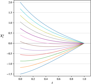
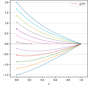
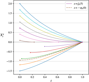
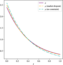
Figure 1: Evolution of the equilibrium state processes without constraint (top-left), with market drop-out (top-right) and with trading constraint (bottom-left) for several representative players. We have highlighted the moments of market entry and drop-out and the initial position $x=-\psi_{\mu}(0)$ and $x=\phi_{\mu}(T)$ (which represent the smallest initial positions for which one has immediate entry, respectively no early exit). In the bottom-right plot we compare the evolution of the mean trading rates of all three scenarios.

To approximate the mean-field equilibrium numerically, we first apply a standard numerical solver to integrate the backward equation (3.13) across varying values of $(\theta,c)$. Subsequently, we employ a standard root-finding procedure to identify a pair $(\theta,c)\in(0,\mathbb{E}[\nu]\frac{\widetilde{\alpha}^{\delta}_{T}}{\eta_{T}})\times[0,Q^{-1}(\mathbb{E}[\nu]))$ that satisfies the equation (3.14), effectively finding a root of the function $\rho:\mathbb{R}^{2}\to\mathbb{R}^{2}$ as defined in the proof of Theorem 3.7.(ii).

Remark 4.1.

For the benchmark case of constant coefficients, a closed-form solution $A^{\delta}$ for the Ricatti equation (2.8) is available (see [20]), which substantially simplifies the numerical implementation.

We first consider an MFG with exponentially distributed initial positions on both sides of the market, setting

$$q(x)=0.8\cdot e^{-\frac{2}{3}x}\quad\mbox{and}\quad p(x)=0.2\cdot e^{x}.$$

This results in an average initial position of $\mathbb{E}[\nu]=1$, that is, in a seller dominated market. Figure 1 presents the evolution of the equilibrium state processes for all three scenarios: no trading constraints, drop-out constraints and with trading constraints and several representative players.

In models without constraints (top-left) we see that players on both sides of the market change the direction of trading for small initial positions. In a seller dominated market buyers can take advantage of favorable price trends. Hence it is beneficial for both sellers and buyers with small initial positions to (further) sell the asset and then buying it back at favorable prices.

Under the market drop-out constraint (top-right), sellers do not change the direction of trading but may exit the market early. On the buyer side, however, we continue to observe players that initially use an opposite trading direction to benefit from the overall market trend. Our trading constraints avoid such effects. In a model with trading constraints (bottom-left) we see that it is beneficial for buyers with small short position to enter the market at later time points.

Figure 1 (bottom-right) presents a comparison of the average equilibrium trading rate across all three scenarios. With the parameters selected, the deviation in tradings rates is small. This is intuitive as only traders with small initial positions, hence with comparably small impact on the market dynamics, enter the market, respectively, exit the market early.

At the same time, we observe that our trading constraint slightly amplifies the effect previously observed under the market drop-out constraint, namely a slower initial aggregate liquidation, followed by an acceleration in aggregate liquidation halfway through the trading period, in comparison to the model without constraints.

This dynamics can be intuitively understood by considering the impact of small buyers who, in the absence of trading constraints, would initially increase their short positions, thereby generating additional selling pressure. Under our trading constraint, these buyers are restricted to hold their position initially. Thus, there is initially no contribution to the aggregate trading rate, which ultimately also results in a higher aggregate trading rate later in the game as there is no need for buying back initially sold stocks.

Furthermore, we again note that in all three settings the relation $\int_{0}^{T}\mu_{t}\,dt=\mathbb{E}[\nu]$ holds. Hence, the price at the terminal time is the same in all settings.

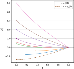
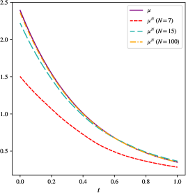
Figure 2: left: Evolution of states of $N=7$ players in the Nash equilibrium. right: Comparison of the mean trading rate in the equilibrium of the MFG (solid line) and the $N$-player game (dashed/dotted line) for $N=7,15$ and $100$.

Figure 2 (left) illustrates the resolution of an $N$-player game with seven players. In this setup, the two buyers both have a starting position above $x=-\psi_{\mu}(0)$ and thus delay their market entry. The two sellers with initial positions below the threshold $x=\phi_{\mu}(0)$ fully liquidate their trades before reaching the terminal time. Figure 2 (right) shows the aggregate rates for several numbers of players. This simulation further supports the observation of a fast convergence to the MFG equilibrium.

5 Conclusion

We established existence and uniqueness of equilibrium results in multi-player and mean-field games of portfolio liquidation under a “no change of trading condition”. We proved that the games are equivalent to games of timing where buyers and sellers need to determine the equilibrium market entry and exit times. Several avenues are open for future research.

First, we worked under the assumption of deterministic market parameters. Although it would clearly be desirable to allow for stochastic parameters, it is unclear to us how to extend our model to the stochastic case. In our setting, entry and exit times are deterministic. In stochastic settings these times were stopping times and our equilibrium analysis would require fixed-point results for stopping times, which is challenging for many reasons. Most importantly we are unaware of any topology on the set of stopping times that would guarantee that (i) the set of stopping times is compact, and at the same time that (ii) our response functions mapping anticipated entry and exit times into actual entry and exit times would be continuous.

A second limitation that one would like to overcome is our assumption that all players share the same liquidation time. In [21] we illustrate how our current results could be used to solve finite player games with heterogeneous trading horizons but the approach is tedious and not very elegant. It would be desirable to develop a general game-theoretic framework that allows for heterogeneous liquidation times.

Appendix A Proof of Proposition 2.7

Let us first note that the function $\widetilde{A}:=e^{-\int_{0}^{\cdot}\frac{\delta\kappa}{\eta_{r}}dr}(A^{\delta}-\delta\kappa)$ satisfies the Riccati equation

$$-\dot{\widetilde{A}}=-\frac{\widetilde{A}^{2}}{\widetilde{\eta}}+\widetilde{\lambda}_{t},\quad t\in[0,T)\qquad\lim_{t\to T}\widetilde{A}_{t}=\infty,$$

with $\widetilde{\eta}=\eta e^{-\int_{0}^{\cdot}\frac{\delta\kappa}{\eta_{r}}dr}$ and $\widetilde{\lambda}=\lambda e^{-\int_{0}^{\cdot}\frac{\delta\kappa}{\eta_{r}}dr}$. Hence, by [21, Lemma A.1] we see that

$$A^{\delta}_{t}-\delta\kappa~{}\geq~{}e^{\int_{0}^{t}\frac{\delta\kappa}{\eta_{r}}dr}A^{\circ}_{t},\qquad t\in[0,T),$$ (A.1)

where $A^{\circ}=(\int_{\cdot}^{T}\frac{1}{\widetilde{\eta}_{s}}ds)^{-1}$. This implies that $A^{\delta}-\delta\kappa$ is positive and bounded away from zero. Using furthermore [21, Lemma A.4] we conclude that the function $\alpha^{\delta}$ is positive, bounded and differentiable.

Next, we prove that condition (i) and (ii) are sufficient for $\psi^{\delta,\tau}_{\mu}$ to be strictly decreasing. Differentiation of $(\alpha^{\delta})^{-1}$ yields that

$$\left(\frac{1}{\alpha^{\delta}_{t}}\right)^{\prime} =e^{\int_{0}^{t}\frac{A^{\delta}_{r}}{\eta_{r}}\,dr}\left(\frac{-\frac{(A^{\delta}_{t})^{2}}{\eta_{t}}+\delta\frac{\kappa}{\eta_{t}}+\lambda_{t}}{(A^{\delta}_{t}-\delta\kappa)^{2}}+\frac{\frac{A^{\delta}_{t}}{\eta_{t}}}{A^{\delta}_{t}-\delta\kappa}\right)~{}=~{}\frac{\lambda_{t}}{(A^{\delta}_{t}-\delta\kappa)\alpha^{\delta}_{t}}.$$

Hence, for the derivative of $\psi^{\delta,\tau}_{\mu}$ we obtain

$$\begin{split}\dot{\psi}^{\delta,\tau}_{\mu}(t)&=~{}\frac{\lambda_{t}}{(A^{\delta}_{t}-\delta\kappa_{t})\alpha^{\delta}_{t}}\int_{t}^{\tau}e^{-\int_{0}^{s}\frac{A^{\delta}_{r}}{\eta_{r}}\,dr}\kappa\mu_{s}\,ds-\frac{1}{A^{\delta}_{t}-\delta\kappa}\kappa\mu_{t}\\ &=~{}\frac{1}{A^{\delta}_{t}-\delta\kappa}(\lambda_{t}\psi_{\mu}(t)-\kappa\mu_{t}).\end{split}$$ (A.2)

Using that the function $\mu\eta$ satisfies Assumption 2.4.(ii) we estimate

$$\dot{\psi}^{\delta,\tau}_{\mu}(t) =\frac{1}{A^{\delta}_{t}-\delta\kappa}\left(\frac{\lambda_{t}}{\alpha^{\delta}_{t}}\int_{t}^{\tau}e^{-\int_{0}^{s}\frac{A^{\delta}_{r}}{\eta_{r}}\,dr}\kappa\mu_{s}\,ds-\kappa\mu_{t}\right)$$

$$\leq\frac{\kappa}{A^{\delta}_{t}-\delta\kappa}\eta_{t}\mu_{t}\left(\frac{\lambda_{t}}{\alpha^{\delta}_{t}}\int_{t}^{T}e^{-\int_{0}^{s}\frac{A^{\delta}_{r}}{\eta_{r}}\,dr}\frac{1}{\eta_{s}}\,ds-\frac{1}{\eta_{t}}\right),$$

for all $t\in[0,\tau]$. It thus suffices to show that the term in the above bracket is strictly negative assuming either (i) or (ii).

• In this case, we use (A.1) to directly estimate

  $$\frac{\lambda_{t}}{\alpha^{\delta}_{t}}\int_{t}^{T}e^{-\int_{0}^{s}\frac{A^{\delta}_{r}}{\eta_{r}}\,dr}\frac{1}{\eta_{s}}\,ds \leq\lambda_{t}\frac{e^{-\int_{0}^{t}\frac{\delta\kappa}{\eta_{r}}dr}}{A^{\circ}_{t}}\int_{t}^{T}e^{-\int_{t}^{s}\frac{A^{\delta}_{r}}{\eta_{r}}\,dr}\frac{1}{\eta_{s}}\,ds$$

  $$=\lambda_{t}\frac{1}{A^{\circ}_{t}}\int_{t}^{T}e^{-\int_{t}^{s}\frac{A^{\delta}_{r}-\delta\kappa}{\eta_{r}}\,dr}\frac{e^{-\int_{0}^{s}\frac{\delta\kappa}{\eta_{r}}dr}}{\eta_{s}}\,ds$$

  $$\leq\lambda_{t}\frac{1}{A^{\circ}_{t}}\int_{t}^{T}e^{-\int_{t}^{s}\frac{A^{\circ}_{r}}{\widetilde{\eta}_{r}}\,dr}\frac{e^{-\int_{0}^{s}\frac{\delta\kappa}{\eta_{r}}dr}}{\eta_{s}}\,ds$$

  $$=\lambda_{t}\frac{1}{A^{\circ}_{t}}\int_{t}^{T}\frac{\int_{s}^{T}\frac{1}{\widetilde{\eta}_{u}}\,du}{\int_{t}^{T}\frac{1}{\widetilde{\eta}_{u}}\,du}\frac{e^{-\int_{0}^{s}\frac{\delta\kappa}{\eta_{r}}dr}}{\eta_{s}}\,ds$$

  $$\leq\lambda_{t}\int_{t}^{T}\frac{1}{\widetilde{\eta}_{s}}\int_{s}^{T}\frac{1}{\widetilde{\eta}_{u}}\,du\,ds$$

  $$\leq\lambda_{t}\frac{1}{2}\left(\int_{t}^{T}\frac{1}{\widetilde{\eta}_{u}}\,du\right)^{2}$$

  for all $t\in[0,\tau]$. We readily conclude when $\|\lambda\|_{\infty}<\frac{2\|\eta^{-1}\|_{\infty}}{T^{2}\|\widetilde{\eta}^{-1}\|_{\infty}^{2}}$.

• In this case we consider the function

  $$z(t):=\frac{1}{\alpha^{\delta}_{t}}\int_{t}^{T}e^{-\int_{0}^{s}\frac{A^{\delta}_{r}}{\eta_{r}}\,dr}\frac{1}{\eta_{s}}\,ds,\qquad 0\leq t\leq T.$$

  Differentiation yields for all $0\leq t<T$ that

  $$\dot{z}(t)= \frac{\lambda_{t}e^{\int_{0}^{t}\frac{A^{\delta}_{r}}{\eta_{r}}\,dr}}{(A_{t}-\delta\kappa)^{2}}\int_{t}^{T}e^{-\int_{0}^{s}\frac{A^{\delta}_{r}}{\eta_{r}}\,dr}\frac{1}{\eta_{s}}\,ds-\frac{1}{\alpha^{\delta}_{t}}e^{-\int_{0}^{t}\frac{A^{\delta}_{r}}{\eta_{r}}\,dr}\frac{1}{\eta_{t}}$$

  $$=\frac{\lambda_{t}}{(A^{\delta}_{t}-\delta\kappa)\alpha^{\delta}_{t}}\int_{t}^{T}e^{-\int_{0}^{s}\frac{A^{\delta}_{r}}{\eta_{r}}\,dr}\frac{1}{\eta_{s}}\,ds-\frac{1}{A^{\delta}_{t}-\delta\kappa}\frac{1}{\eta_{t}}$$

  $$=\frac{1}{(A^{\delta}_{t}-\delta\kappa)\eta_{t}}\left(\lambda_{t}\eta_{t}z(t)-1\right).$$

  If we can prove that

  $$t_{0}:=\sup\left\{t\in[0,T]\;|\;z(t)\lambda_{t}\eta_{t}=1\right\}=-\infty,$$

  then we have for all $t\in[0,T]$ that

  $$\frac{\lambda_{t}}{\alpha^{\delta}_{t}}\int_{t}^{T}e^{-\int_{0}^{s}\frac{A^{\delta}_{r}}{\eta_{r}}\,dr}\frac{1}{\eta_{s}}\,ds=z(t)\lambda_{t}<\frac{1}{\eta_{t}}$$

  and the claim readily follows. Since, $z(T)=0$ it holds that $t_{0}<T$. Let us now assume to the contrary that $t_{0}\geq 0$. Then $\lambda_{t_{0}}>0$, $z(t_{0})=\frac{1}{\lambda_{t_{0}}\eta_{t_{0}}}$, $\dot{z}(t_{0})=0$ and

  $$z(t)<\frac{1}{\lambda_{t}\eta_{t}}\quad\mbox{for all}\quad t\in({t_{0}},T].$$

  Since $(\lambda\eta)$ is non-decreasing $\dot{z}(t)\geq\frac{1}{(A^{\delta}_{t}-\delta\kappa)\eta_{t}}(\lambda_{t_{0}}\eta_{t_{0}}z(t)-1)$ on $[t_{0},T)$ and hence we have for all $t\in[t_{0},T)$

  $$\left(z(t)-\frac{1}{\lambda_{t_{0}}\eta_{t_{0}}}\right)^{\prime}\geq\frac{\lambda_{t_{0}}\eta_{t_{0}}}{(A^{\delta}_{t}-\delta\kappa)\eta_{t}}\left(z(t)-\frac{1}{\lambda_{t_{0}}\eta_{t_{0}}}\right).$$

  By Grönwall’s inequality this shows that

  $$z(t)-\frac{1}{\lambda_{t_{0}}\eta_{t_{0}}}\geq\left(z(t_{0})-\frac{1}{\lambda_{t_{0}}\eta_{t_{0}}}\right)e^{\int_{t_{0}}^{t}\frac{\lambda_{t_{0}}\eta_{t_{0}}}{(A^{\delta}_{s}-\delta\kappa)\eta_{s}}\,ds}=0$$

  and hence $z(t)\geq\frac{1}{\lambda_{t_{0}}\eta_{t_{0}}}\geq\frac{1}{\lambda_{t}\eta_{t}}$ on $[t_{0},T)$, which contradicts the definition of $t_{0}$.

Appendix B Representation of the function $\cal J$ and derivative of $\vartheta^{\theta,c}$

In this appendix we prove two auxiliary results that are needed to solve our fixed-point equation. We start with the following result that establishes the alternative representation of the function ${\cal J}$ defined in (3.16).

Lemma B.1.

The map ${\cal J}:C^{0}([0,T])\to C^{0}([0,T])$ defined in (3.16) satisfies the representation (3.18).

Proof.

We recall that for any $\vartheta\in C^{0}([0,T])$ it holds that

$${\cal J}(\vartheta)_{t}=\int_{t}^{T}(p\left(-\psi_{\vartheta/\eta}(s)\right)-\delta)\pi_{s}\vartheta_{s}\,ds+\int_{t}^{T}\lambda_{s}\ell\left(-\psi_{\vartheta/\eta}(s)\right)\,ds,\qquad t\in[0,T].$$

Using that $\ell(x)=xp(x)-P(x)$ for all $x\leq 0$ and furthermore that

$$\dot{\psi}_{\vartheta/\eta}(t)=\frac{1}{A^{\delta}_{t}-\delta\kappa}\left(\lambda_{t}\psi_{\vartheta/\eta}(t)-\pi_{t}\vartheta_{t}\right),\quad t\in[0,T],$$

we have that

$${\cal J}(\vartheta)_{t}= ~{}-\int_{t}^{T}(A^{\delta}_{s}-\delta\kappa)p(-\psi_{\vartheta/\eta}(s)\big{)}\dot{\psi}_{\vartheta/\eta}(s)\,ds-\int_{t}^{T}\delta\pi_{s}\vartheta_{s}\,ds$$

$$\quad-\int_{t}^{T}\lambda_{s}P(-\psi_{\vartheta/\eta}(s))ds,\qquad t\in[0,T].$$

We now use integration by parts to obtain that

$$~{}-\int_{t}^{T}(A^{\delta}_{s}-\delta\kappa)p(-\psi_{\vartheta/\eta}(s))\dot{\psi}_{\vartheta/\eta}(s)\,ds$$

$$= ~{}\left.(A^{\delta}_{s}-\delta\kappa)P(-\psi_{\vartheta/\eta}(s))\right|_{s=t}^{T}-\int_{t}^{T}\dot{A}^{\delta}_{s}P(-\psi_{\vartheta/\eta}(s)\,ds$$

$$= ~{}-(A^{\delta}_{t}-\delta\kappa)P(-\psi_{\mu}(t))-\int_{t}^{T}\left(\frac{(A^{\delta}_{s})^{2}}{\eta_{s}}-\frac{\delta\kappa}{\eta_{s}}A^{\delta}_{s}-\lambda_{s}\right)P(-\psi_{\mu}(s))ds,\quad t\in[0,T],$$

where we have used that the limit of the first term in the right-hand side is zero as $t\to T$, which can be obtained by using L’Hospital’s rule. Plugging this into the above representation for ${\cal J}$ we then obtain the desired result. ∎

The next lemma proves the differentiability of the solution $\vartheta^{\theta,c}\in C([0,T])$ to the (3.15) with respect to the parameters $\theta$ and $c$ and establishes uniform bounds for the partial derivatives. The key observation is that the derivatives satisfy a non-standard Volterra equation with possibly unbounded kernel.

We recall that the map $\rho:[0,\infty)\times[0,\infty)\to\mathbb{R}^{2}$ is defined by

$$\rho_{1}(\theta,c) =\frac{\eta_{T}}{\widetilde{\alpha}^{\delta}_{T}}\theta-\mathbb{E}[\nu]+Q(c)-\int_{0}^{T}e^{\int_{0}^{t}\frac{A^{\delta}_{r}-\delta\kappa}{\eta_{r}}dr}\frac{A^{\delta}_{t}-\delta\kappa}{\eta_{t}}P\left(-\frac{1}{\alpha^{\delta}_{t}}\int_{t}^{T}e^{-\int_{0}^{u}\frac{A^{\delta}_{r}}{\eta_{r}}\,dr}\pi_{u}\vartheta^{\theta,c}_{u}\,du\right)\,dt,$$

$$\rho_{2}(\theta,c) =c-\int_{0}^{T}h^{\delta}_{s}\pi_{s}\vartheta^{\theta,c}_{s}\,ds.$$

Lemma B.2.

The map $(\theta,c)\mapsto\vartheta^{\theta,c}_{t}$ is differentiable for all $t\in(0,T]$ and there exists a constant $K>0$ depending only on $T,\lambda,\kappa$ and $\eta$ such that

$$0~{}<~{}\eta_{T}~{}\leq~{}\frac{\partial\vartheta^{\theta,c}_{t}}{\partial\theta}~{}\leq~{}K\frac{1}{h^{\delta}_{t}}\qquad\text{ and }\qquad-K\frac{1}{h^{\delta}_{t}}~{}\leq~{}\frac{\partial\vartheta^{\theta,c}_{t}}{\partial c}~{}\leq~{}0,\qquad t\in(0,T],\quad\theta,c\geq 0.$$

Furthermore, $\rho$ is differentiable and

$$D\rho_{(\theta,c)}=\begin{pmatrix}\frac{\eta_{T}}{\widetilde{\alpha}^{\delta}_{T}}+\int_{0}^{T}\chi_{s}\frac{\partial\vartheta^{\theta,c}_{s}}{\partial c}\,ds&q(c)+\int_{0}^{T}\chi_{s}\frac{\partial\vartheta^{\theta,c}_{s}}{\partial c}\,ds\\ -\int_{0}^{T}h^{\delta}_{s}\pi_{s}\frac{\partial\vartheta^{\theta,c}_{s}}{\partial\theta}ds&1-\int_{0}^{T}h^{\delta}_{s}\pi_{s}\frac{\partial\vartheta^{\theta,c}_{s}}{\partial c}\,ds\end{pmatrix}$$

where for all $t\in[0,T]$

$$0~{}\leq~{}\chi_{t}:=\pi_{t}e^{-\int_{0}^{t}\frac{A^{\delta}_{r}}{\eta_{r}}\,dr}\int_{0}^{t}\frac{e^{2\int_{0}^{s}\frac{A^{\delta}_{r}-\delta\kappa}{\eta_{r}}\,dr}}{\eta_{s}}p\left(-\frac{1}{\alpha^{\delta}_{s}}\int_{s}^{T}e^{-\int_{0}^{u}\frac{A^{\delta}_{r}}{\eta_{r}}\,dr}\pi_{u}\vartheta^{\theta,c}_{u}\,du\right)\,ds~{}\leq~{}Kp(0)h^{\delta}_{t}.$$

Proof.

In what follows $K>0$ denotes a constant that may change from line to line but only depends on $T,\kappa,\eta$, $\lambda$. Our starting point is the equation (3.15), which can be brought into the following form using an integration by parts argument (cf. Lemma B.1):

$$\begin{split}\vartheta_{t}=~{}&\theta\eta_{T}+\frac{1}{h^{\delta}_{T}}Q\left(c\right)-\frac{1}{h^{\delta}_{t}}Q\left(c-\int_{t}^{T}h^{\delta}_{u}\pi_{u}\vartheta_{u}du\right)+\int_{t}^{T}\frac{\dot{h}^{\delta}_{s}}{(h^{\delta}_{s})^{2}}Q\left(c-\int_{s}^{T}h^{\delta}_{u}\pi_{u}\vartheta_{u}du\right)\,ds\\ &-(A^{\delta}_{t}-\delta\kappa)P\left(-\frac{1}{\alpha^{\delta}_{s}}\int_{s}^{T}e^{-\int_{0}^{u}\frac{A^{\delta}_{r}}{\eta_{r}}\,dr}\pi_{u}\vartheta_{u}\,du\right)\\ &-\int_{t}^{T}\frac{A_{s}^{\delta}(A^{\delta}_{s}-\delta\kappa)}{\eta_{s}}P\left(-\frac{1}{\alpha^{\delta}_{s}}\int_{s}^{T}e^{-\int_{0}^{u}\frac{A^{\delta}_{r}}{\eta_{r}}\,dr}\pi_{u}\vartheta_{u}\,du\right)\,ds\\ &+\int_{t}^{T}\lambda_{s}\left(\int_{s}^{T}\frac{1}{\eta_{u}}\vartheta_{u}\,du\right)\,ds-\int_{t}^{T}\delta\pi_{s}\vartheta_{s}\,ds.\end{split}$$ (B.1)

By the proof (i) of Theorem 3.7, we know that for any $\theta,c\geq 0$ there exists a unique solution

$$\vartheta^{\theta,c}\in C^{0}([0,T])$$

to the above equation and the estimates (3.19) and (3.20) show that the mapping

$$(\theta,c)\mapsto\vartheta^{\theta,c}|_{[\varepsilon,T]}\in C^{0}([\varepsilon,T])$$

is Lipschitz continuous, for any $\varepsilon>0$. This allows us to apply the dominated convergence theorem to establish the differentiability w.r.t. $\theta$ and to interchange differentiation and integration to obtain the following representation of the derivative:

$$\begin{split}\frac{\partial\vartheta^{\theta,c}_{t}}{\partial\theta}=&~{}\eta_{T}+\frac{1}{h^{\delta}_{t}}q\left(c-\int_{t}^{T}h^{\delta}_{s}\pi_{s}\vartheta^{\theta,c}_{s}\,ds\right)\int_{t}^{T}h^{\delta}_{s}\pi_{s}\frac{\partial\vartheta^{\theta,c}_{s}}{\partial\theta}\,ds\\ &-\int_{t}^{T}\frac{\dot{h}^{\delta}_{s}}{(h_{s}^{\delta})^{2}}q\left(c-\int_{s}^{T}h^{\delta}_{u}\pi_{u}\vartheta^{\theta,c}_{u}\,du\right)\left(\int_{s}^{T}h^{\delta}_{u}\pi_{u}\frac{\partial\vartheta^{\theta,c}_{u}}{\partial\theta}\,du\right)\,ds\\ &+(A^{\delta}_{t}-\delta\kappa)p\left(-\frac{1}{\alpha^{\delta}_{t}}\int_{t}^{T}e^{-\int_{0}^{u}\frac{A^{\delta}_{r}}{\eta_{r}}\,dr}\pi_{u}\vartheta^{\theta,c}_{u}\,du\right)\frac{1}{\alpha^{\delta}_{t}}\int_{t}^{T}e^{-\int_{0}^{s}\frac{A^{\delta}_{r}}{\eta_{r}}\,dr}\pi_{s}\frac{\partial\vartheta^{\theta,c}_{s}}{\partial\theta}\,ds\\ &+\int_{t}^{T}\frac{A^{\delta}_{s}(A^{\delta}_{s}-\delta\kappa)}{\eta_{s}}p\left(-\frac{1}{\alpha^{\delta}_{s}}\int_{s}^{T}e^{-\int_{0}^{u}\frac{A^{\delta}_{r}}{\eta_{r}}\,dr}\pi_{u}\vartheta^{\theta,c}_{u}\,du\right)\frac{1}{\alpha^{\delta}_{s}}\left(\int_{s}^{T}e^{-\int_{0}^{u}\frac{A^{\delta}_{r}}{\eta_{r}}\,dr}\pi_{u}\frac{\partial\vartheta^{\theta,c}_{u}}{\partial\theta}\,du\right)\,ds\\ &+\int_{t}^{T}\lambda_{s}\left(\int_{s}^{T}\frac{1}{\eta_{u}}\frac{\partial\vartheta^{\theta,c}_{u}}{\partial\theta}\,du\right)\,ds-\int_{t}^{T}\delta\pi_{s}\frac{\partial\vartheta^{\theta,c}_{s}}{\partial\theta}\,ds\\ =:&~{}\eta_{T}+\int_{t}^{T}\Gamma(t,s)\frac{\partial\vartheta^{\theta,c}_{s}}{\partial\theta}\,ds,\end{split}$$ (B.2)

where the kernel $\Gamma$ admits the explicit representation

$$\Gamma(t,s)~{}= ~{}\frac{h^{\delta}_{s}\pi_{s}}{h^{\delta}_{t}}C_{t}-h^{\delta}_{s}\pi_{s}\int_{t}^{s}\frac{\dot{h}^{\delta}_{u}}{(h^{\delta}_{u})^{2}}C_{u}\,du+\frac{1}{\eta_{s}}\int_{t}^{s}\lambda_{u}\,du$$

$$+D_{t}e^{-\int_{t}^{s}\frac{A^{\delta}_{r}}{\eta_{r}}\,dr}\pi_{s}+e^{-\int_{0}^{s}\frac{A^{\delta}_{r}}{\eta_{r}}\,dr}\pi_{s}\int_{t}^{s}\frac{A^{\delta}_{u}(A^{\delta}_{u}-\delta\kappa)}{\eta_{u}}D_{u}\frac{1}{\alpha^{\delta}_{u}}\,du-\delta\pi_{s}$$

for all $0\leq t\leq s\leq T$ with

$$C_{t}:=q\left(c-\int_{t}^{T}h^{\delta}_{s}\pi_{s}\vartheta^{\theta,c}_{s}\,ds\right),\quad D_{t}:=p\left(-\frac{1}{\alpha^{\delta}_{t}}\int_{t}^{T}e^{-\int_{0}^{u}\frac{A^{\delta}_{r}}{\eta_{r}}\,dr}\pi_{u}\vartheta^{\theta,c}_{u}\,du\right).$$

This shows that the derivative satisfies a Volterra integral equation, which suggests that the derivative can be bounded in terms of the kernel $\Gamma$. To this end, we first prove that $\Gamma$ non-negative and then establish a growth condition on the kernel that carries over to our derivative function.

• Non-negativity of $\Gamma$. The function $C$ is càglàd and non-increasing, and thus of finite variation. Moreover, $h^{\delta}$ is continuous and increasing. Therefore, using the integration by parts formula for finite variation functions we can transform the first two terms of $\Gamma$ as follows

  $$\frac{h^{\delta}_{s}\pi_{s}}{h_{t}}C_{t}-h^{\delta}_{s}\pi_{s}\int_{t}^{s}\frac{\dot{h}^{\delta}_{u}}{(h_{u}^{\delta})^{2}}C_{u}\,du{-\delta\pi_{s}}~{}=~{}\pi_{s}(C_{s}{-\delta})-h^{\delta}_{s}\pi_{s}\int_{[t,s)}\frac{1}{h^{\delta}_{u}}\,dC_{u},\quad 0<t\leq s\leq T.$$

  In the MFG $\delta=0$ and hence the above term is non-negative. In the $N$-player game $\delta=\frac{1}{N}$. Let $x_{N}$ be the initial position of the largest seller, i.e. the upper limit of the support of $\nu$. Since

  $$c-\int_{s}^{T}h^{\delta}_{r}\pi_{r}\vartheta^{\theta,c}_{r}\,dr\leq c<Q^{-1}(\mathbb{E}[\nu])\leq Q^{-1}(\mathbb{E}[\nu|_{[0,\infty]}])=x_{N},$$

  we see that

  $$C_{s}=q\left(c-\int_{t}^{T}h^{\delta}_{s}\pi_{s}\vartheta^{\theta,c}_{s}\,ds\right)\geq\frac{1}{N}$$

  from which we again deduce non-negativity of the above term. All other terms in the definition of $\Gamma$ are non-negative as well.

• Growth bounds on $\Gamma$. Using again that $h^{\delta}$ is increasing we see that

  $$\left|\pi_{s}C_{s}-h^{\delta}_{s}\pi_{s}\int_{[t,s)}\frac{1}{h^{\delta}_{u}}\,dC_{u}\right|~{}\leq~{}K\left(1+\frac{h^{\delta}_{s}}{h^{\delta}_{t}}\right),\qquad 0<t\leq s\leq T.$$

  By [21, Lemma A.1] we have the following estimate

  $$e^{-\int_{0}^{s}\frac{A^{\delta}_{r}}{\eta_{r}}\,dr}\pi_{s}\int_{t}^{s}\frac{(A^{\delta}_{u})^{2}}{\eta_{u}}D_{u}\frac{1}{\alpha^{\delta}_{u}}\,du~{}\leq~{}K(T-s)\int_{t}^{s}\frac{1}{(T-u)^{2}}\,du~{}\leq~{}K,\qquad 0\leq t\leq s\leq T.$$

From the above estimates and the monotonicity of $h^{\delta}$ it follows that the modified kernel

$$\widetilde{\Gamma}(t,s):=\Gamma(t,s)\frac{h^{\delta}_{t}}{h^{\delta}_{s}},\qquad 0\leq t\leq s\leq T$$

is non-negative and bounded. Results established in [5] show that

$$y(t):=h^{\delta}_{t}\frac{\partial{\vartheta^{\theta,c}_{t}}}{\partial\theta},\quad t\in[0,T]$$

is the unique and bounded solution to the Volterra integral equation

$$y(t)= ~{}h^{\delta}_{t}\eta_{T}+\int_{t}^{T}\widetilde{\Gamma}(t,s)y(s)\,ds,\quad t\in[0,T].$$

In particular, there exists a constant $K>0$ such that

$$\eta_{T}~{}\leq~{}\frac{\partial{\vartheta^{\theta,c}_{t}}}{\partial\theta}~{}\leq~{}K\frac{1}{h^{\delta}_{t}},\qquad 0<t\leq T.$$

An analogous argument establishes the differentiability of the function $\vartheta^{\theta,c}_{t}$ with respect to the parameter $c$ and shows that

$$y(t)=h^{\delta}_{t}\frac{\partial{\vartheta^{\theta,c}_{t}}}{\partial c},\quad t\in[0,T]$$

uniquely solves the integral equation

$$y(t)= ~{}z(t)+\int_{t}^{T}\widetilde{\Gamma}(t,s)y(s)\,ds,\quad t\in[0,T],$$

where

$$z(t):=h^{\delta}_{t}\left(\frac{1}{h^{\delta}_{T}}q\left(c\right)-\frac{1}{h^{\delta}_{t}}C_{t}+\int_{t}^{T}\frac{\dot{h}^{\delta}_{s}}{(h^{\delta}_{s})^{2}}C_{s}\,ds\right)~{}=~{}h^{\delta}_{t}\int_{[t,T)}\frac{1}{h^{\delta}_{u}}\,dC^{\delta}_{u}.$$

As before we see from the right-hand side that $z$ is non-positive and bounded. Hence, it follows that

$$-K\frac{1}{h^{\delta}_{t}}~{}\leq~{}\frac{\partial{\vartheta^{\theta,c}_{t}}}{\partial c}~{}\leq~{}z(t)\frac{1}{h^{\delta}_{t}}\leq 0,\qquad 0<t\leq T.$$

To prove that $\rho$ is differentiable we have to once again justify that differentiation w.r.t. $\theta$ (resp. $c$) is interchangeable with the integrals in the definition of $\rho$.

To this end, we notice that the above bounds for $\left|\frac{\partial{\vartheta^{\theta,c}}}{\partial\theta}\right|$ and $\left|\frac{\partial{\vartheta^{\theta,c}}}{\partial c}\right|$ hold uniformly in $\theta,c\geq 0$. Thus it suffices to show that these bounds provide integrable majorants. For $\rho_{2}$ this follows from the presence of the factor $h^{\delta}$ in the integrand. Regarding $\rho_{1}$ we recall that by [21, Lemma 2.6] we have that $h^{\delta}_{t}\geq Kt$ for all $t\geq 0$ and thus,

$$\int_{0}^{T}\frac{A^{\delta}_{t}-\delta\kappa}{\alpha^{\delta}_{t}\eta_{t}}p\left(-\frac{1}{\alpha^{\delta}_{t}}\int_{t}^{T}e^{-\int_{0}^{u}\frac{A^{\delta}_{r}}{\eta_{r}}\,dr}\pi_{u}\vartheta^{\theta,c}_{u}\,du\right)e^{\int_{0}^{t}\frac{A^{\delta}_{r}-\delta\kappa}{\eta_{r}}\,dr}\left(\int_{t}^{T}e^{-\int_{0}^{s}\frac{A^{\delta}_{r}}{\eta_{r}}\,dr}\pi_{s}\frac{1}{h_{s}}\,ds\right)\,dt$$

$$\leq K\int_{0}^{T}(A^{\delta}_{t}-\delta\kappa)\left(\int_{t}^{T}\frac{1}{s}ds\right)\,dt$$

$$\leq K\int_{0}^{T}\frac{1}{T-t}(\log(T)-\log(t))\,dt$$

$$<\infty.$$

A straightforward computation using Fubini’s theorem now shows that

$$\frac{\partial\rho_{1}}{\partial\theta}(\theta,c)= ~{}\frac{\eta_{T}}{\widetilde{\alpha}^{\delta}_{T}}+\int_{0}^{T}\frac{A^{\delta}_{t}-\delta\kappa}{\alpha^{\delta}_{t}\eta_{t}}p\left(-\frac{1}{\alpha^{\delta}_{t}}\int_{t}^{T}e^{-\int_{0}^{u}\frac{A^{\delta}_{r}}{\eta_{r}}\,dr}\pi_{u}\vartheta^{\theta,c}_{u}\,du\right)e^{\int_{0}^{t}\frac{A^{\delta}_{r}-\delta\kappa}{\eta_{r}}\,dr}$$

$$~{}\qquad\qquad\times\left(\int_{t}^{T}e^{-\int_{0}^{s}\frac{A^{\delta}_{r}}{\eta_{r}}\,dr}\pi_{s}\frac{\partial\vartheta^{\theta,c}_{s}}{\partial\theta}\,ds\right)\,dt$$

$$= ~{}\frac{\eta_{T}}{\widetilde{\alpha}^{\delta}_{T}}+\int_{0}^{T}\frac{\partial\vartheta^{\theta,c}_{t}}{\partial\theta}\pi_{t}e^{-\int_{0}^{t}\frac{A^{\delta}_{r}}{\eta_{r}}\,dr}\left(\int_{0}^{t}e^{\int_{0}^{s}\frac{A^{\delta}_{r}-\delta\kappa}{\eta_{r}}\,dr}\frac{A^{\delta}_{s}-\delta\kappa}{\alpha^{\delta}_{s}\eta_{s}}\right.$$

$$~{}\left.\qquad\qquad\times p\left(-\frac{1}{\alpha^{\delta}_{s}}\int_{s}^{T}e^{-\int_{0}^{u}\frac{A^{\delta}_{r}}{\eta_{r}}\,dr}\pi_{u}\vartheta^{\theta,c}_{u}\,du\right)\,ds\right)\,dt$$

$$= ~{}\frac{\eta_{T}}{\widetilde{\alpha}^{\delta}_{T}}+\int_{0}^{T}\frac{\partial\vartheta^{\theta,c}_{t}}{\partial\theta}\chi^{\theta,c}_{t}\,dt.$$

The derivation of the remaining partial derivatives is analogous. The fact that $\chi^{\theta,c}$ is non-negative follows from its definition while its upper bound follows from the definition of $h$. ∎

References

• [1] R. Aïd, R. Dumitrescu, and P. Tankov. The entry and exit game in the electricity markets: A mean-field game approach. Journal of Dynamics and Games, 8(4):331–358, 2021.
• [2] R. Almgren and N. Chriss. Optimal execution of portfolio transactions. Journal of Risk, 3:5–40, 2001.
• [3] S. Ankirchner, M. Jeanblanc, and T. Kruse. BSDEs with singular terminal condition and a control problem with constraints. SIAM Journal on Control and Optimization, 52(2):893–913, 2014.
• [4] P. Bank and M. Voß. Linear quadratic stochastic control problems with singular stochastic terminal constraint. SIAM Journal on Control and Optimization, 56(2):672–669, 2018.
• [5] P. R. Beesack. Comparison theorems and integral inequalities for Volterra integral equations. Proc. Am. Math. Soc., 20:61–66, 1969.
• [6] J. F. Bonnans, J. Gianatti, and L. Pfeiffer. A Lagrangian approach for aggregative mean field games of controls with mixed and final constraints. SIAM Journal on Control and Optimization, 61(1):105–134, 2023.
• [7] G. Bouveret, R. Dumitrescu, and P. Tankov. Mean-field games of optimal stopping: A relaxed solution approach. SIAM Journal on Control and Optimization, 58(4):1795–1821, 2020.
• [8] L. Campi and M. Burzoni. Mean field games with absorption and common noise with a model of bank run. Stochastic Processes and Their Applications, 164:206–241, 2023.
• [9] L. Campi and M. Fischer. $N$-player games and mean-field games with absorption. Annals of Applied Probability, 28(4):2188–2242, 2018.
• [10] L. Campi, M. Ghio, and G. Livieri. $N$-player games and mean-field games with smooth dependence on past absorptions. Annales de l’Institut Henri Poincaré, 57(4):1901–1939, 2021.
• [11] P. Cardaliaguet and C. Lehalle. Mean field game of controls and an application to trade crowding. Mathematics and Financial Economics, 12(3):335–363, 2018.
• [12] B. Carlin, M. Lobo, and S. Viswanathan. Episodic liquidity crises: Cooperative and predatory trading. Journal of Finance, 62(5):2235–2274, 2007.
• [13] R. Carmona, F. Delarue, and D. Lacker. Mean field games of timing and models for bank runs. Applied Mathematics & Optimization, 76(1):217–260, 2017.
• [14] P. Casgrain and S. Jaimungal. Mean field games with partial information for algorithmic trading. arXiv:1803.04094, 2018.
• [15] P. Casgrain and S. Jaimungal. Mean-field games with differing beliefs for algorithmic trading. Mathematical Finance, 30(3):995–1034, 2020.
• [16] R. Cesari and H. Zheng. Stochastic maximum principle for optimal liquidation with control-dependent terminal time. Applied Mathematics and Optimization, 85:43(3), 2022.
• [17] S. Drapeau, P. Luo, A. Schied, and D. Xiong. An FBSDE approach to market impact games with stochastic parameters. Probability, Uncertainty and Quantitative Risk, 6(3):237–260, 2019.
• [18] R. Dumitrescu, M. Leutscher, and P. Tankov. Control and optimal stopping mean field games: a linear programming approach. Electronic Journal of Probability, 26:1–49, 2021.
• [19] A. Fruth, T. Schöneborn, and M. Urusov. Optimal trade execution and price manipulation in order books with time-varying liquidity. Mathematical Finance, 24(4):651–695, 2014.
• [20] G. Fu, P. Graewe, U. Horst, and A. Popier. A mean field game of optimal portfolio liquidation. Mathematics of Operations Research, 46(4):1251–1281, 2021.
• [21] G. Fu, P. Hager, and U. Horst. Mean-field liquidation games with market drop-out. to appear in Mathematical Finance, 2023.
• [22] G. Fu and U. Horst. Mean-field leader-follower games with terminal state constraint. SIAM Journal on Control and Optimization, 58(4):2078–2113, 2020.
• [23] G. Fu, U. Horst, and X. Xia. A mean-field control problem of optimal portfolio liquidation with semimartingale strategies. to appear in Mathematics of Operations Research, 2022.
• [24] G. Fu, U. Horst, and X. Xia. Portfolio liquidation games with self exciting order flow. Mathematical Finance, 30(4):1020–1065, 2022.
• [25] J. Gatheral and A. Schied. Optimal trade execution under geometric Brownian motion in the Almgren and Chriss framework. International Journal of Theoretical and Applied Finance, 14(3):353–368, 2011.
• [26] P. Graewe and U. Horst. Optimal trade exection with instantaneous price impact and stochastic resilience. SIAM Journal on Control and Optimization, 55(6):3707–3725, 2017.
• [27] P. Graewe, U. Horst, and R. Sircar. A maximum principle approach to a deterministic mean field game of control with absorption. SIAM Journal on Control and Optimization, 60(5):3173–3190, 2022.
• [28] U. Horst. Stationary equilibria in discounted stochastic games with weakly interacting players. Games and Economic Behavior, 51(1):83–108, 2005.
• [29] U. Horst and J. Scheinkman. Equilibria in systems of social interactions. Journal of Economic Theory, 130(1):44–77, 2006.
• [30] U. Horst, X. Xia, and C. Zhou. Portfolio liquidation under factor uncertainty. Annals of Applied Probability, 32(1):80–123, 2022.
• [31] X. Huang, S. Jaimungal, and M. Nourian. Mean-field game strategies for optimal execution. Applied Mathematical Finance, 26:153–185, 2019.
• [32] P. Kratz. An explicit solution of a nonlinear-quadratic constrained stochastic control problem with jumps: Optimal liquidation in dark pools with adverse selection. Mathematics of Operations Research, 39(4):1198–1220, 2014.
• [33] T. Kruse and A. Popier. Minimal supersolutions for BSDEs with singular terminal condition and application to optimal position targeting. Stochastic Processes and their Applications, 126(9):2554–2592, 2016.
• [34] X. Luo and A. Schied. Nash equilibrium for risk-averse investors in a market impact game with transient price impact. Market Microstructure and Liquidity, 5, 2020.
• [35] A. Micheli, J. Muhle-Karbe, and E. Neuman. Closed-loop nash competition for liquidity. Mathematical Finance, 33(4):1082–1118, 2023.
• [36] E. Neuman and M. Voß. Trading with the crowd. Mathematical Finance, 33(3):548–617, 2023.
• [37] M. Nutz. A mean field games of optimal stopping. SIAM Journal on Control and Optimization, 56:1206–1221, 2018.
• [38] A. Obizhaeva and J. Wang. Optimal trading strategy and supply/demand dynamics. Journal of Financial Markets, 16(1):1–32, 2013.
• [39] A. Popier and C. Zhou. Second order BSDE under monotonicity condition and liquidation problem under uncertainty. Annals of Applied Probability, 29(3), 2019.
• [40] A. Schied, E. Strehle, and T. Zhang. High-frequency limit of Nash equilibria in a market impact game with transient price impact. SIAM Journal on Financial Mathematics, 8(1):589–634, 2017.
• [41] A. Schied and T. Zhang. A market impact game under transient price impact. Mathematics of Operations Research, 44(1):102–121, 2019.
• [42] E. Strehle. Optimal execution in a multiplayer model of transient price impact. Market Microstructure and Liquidity, 3(3-4):1850007, 2018.
• [43] G. Teschl. Ordinary Differential Equations and Dynamical Systems. AMS, 2016.