H-MaP: An Iterative and Hybrid Sequential Manipulation Planner

Abstract

This study introduces the Hybrid Sequential Manipulation Planner (H-MaP), a novel approach that iteratively does motion planning using contact points and waypoints for complex sequential manipulation tasks in robotics. Combining optimization-based methods for generalizability and sampling-based methods for robustness, H-MaP enhances manipulation planning through active contact mode switches and enables interactions with auxiliary objects and tools. This framework, validated by a series of diverse physical manipulation tasks and real-robot experiments, offers a scalable and adaptable solution for complex real-world applications in robotic manipulation.
https://sites.google.com/view/h-map/

I INTRODUCTION

Sequential manipulation is crucial since it enables robots to complete complex tasks by executing a series of actions, allowing them to handle multi-step processes. However, sequential manipulation is challenging for robots. The first challenge is creating a generic method for solving various tasks. In sequential manipulation tasks, such as picking the stick and pushing the object (Fig. 1 top-right), the solver should be able to solve the combination of specified actions. Toussaint et al. address this challenge in [1] and propose an optimization-based method that abstracts the actions using kinematic modes. However, this approach has several drawbacks, such as the risk of trapping into local minima since it uses optimization and lacks robustness in manipulation tasks that require contact mode switches dynamically. One example of this case is pushing an object under the tunnel and picking from the other side (Fig. 3-a).

Dynamic contact mode switching is crucial to obtain dexterous manipulation. Therefore, model-based dexterous manipulation solvers usually obtain active mode switches by contact mode sampling, which also helps to reach a global solution [2, 3, 4]. However, current dexterous manipulation methods face the risk of the dimensionality of the configuration space increasing excessively. Therefore, this inhibits their scalability and hinders them from producing long sequence manipulations. Besides, they do not present the applicability of their methods on tool-use and auxiliary object manipulation scenarios.

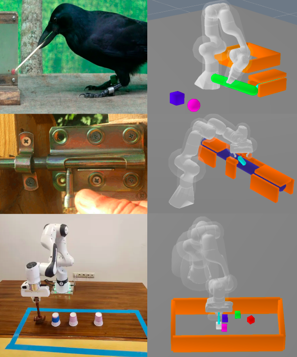
Figure 1: (Left) A crow using a tool to reach the food [5], opening a sliding bolt latch [6]; a Franka Panda robot executing an obstacle removal task with a tool. (Right) Tasks solved by our approach: using a tool to push an object out then pick it up, a latch system, and removing an obstacle with a tool.

Recognizing these challenges in sequential manipulation planning, the physical manipulation capabilities of humans have provided us with some inspiration. In essence, the human brain anticipates the outcomes of interactions with objects in the environment [7], predicts the trajectory of objects [8], and simulates the outcome of an action [9]. Besides, humans inherently decide contact points when manipulating objects [10]. These insights motivate our approach, as presented in this study.

This paper proposes a generic hybrid sequential manipulation planner (H-MaP) that enables complex manipulation planning by using an optimization-based method [11, 12] for generalizability and a sampling-based method for robustness. H-MaP iteratively plans motion using waypoints and contact points. Waypoints and contact points represent the sequential discrete poses of the target object and physical interaction points, respectively. The key idea is the iterative computation of the contact points among waypoints. This iterative approach enhances the robustness of the solver. Waypoints decompose the problem into smaller steps, and contact points guide the motion planner in switching contact modes. Contact modes facilitate the dynamic adjustment of the robot’s interaction with objects during motion planning, guiding the solver on how and where the manipulator should engage or disengage with objects. Combined with an optimization-based planner, waypoint and contact point information enable the solver to accomplish complex sequential manipulation tasks. Thus, our contributions are as follows:

• A hybrid manipulation planner that employs sampling- and optimization-based methods for complex tasks and also facilitates interactions with auxiliary objects and tool use.

• An enhancement in modularity and robustness via an iterative approach that utilizes waypoints and contact points for physical sequential manipulation planning.

Our contributions are showcased through six diverse physical manipulation tasks, complemented by real-robot experiments to confirm the real-world applicability of our method. Primarily, we choose tasks in a constrained environment, such as opening a sliding bolt latch and pushing an object out of a narrow hole with and without using a tool (Fig. 1). These manipulation problems represent the capabilities of our method in complex tasks. We further tested our approach on each scenario by varying parameters (e.g., size and pose) of the objects in environments, demonstrating the robustness of H-MaP.

II Related Work

II-A Optimization-Based Manipulation Planning

Manipulation planning refers to determining a sequence of motions and actions for a robot to interact with objects effectively. Optimization-based manipulation planning, in particular, aims to determine optimal trajectories by minimizing or maximizing a defined objective function within specified constraints, encompassing criteria such as path efficiency, energy conservation, and obstacle avoidance. CHOMP [13] and its variants [14, 15] employ covariant gradient descent to optimize a cost functional. STOMP [16] optimizes non-differentiable costs via stochastic sampling, while TrajOpt [17] employs sequential quadratic programming with continuous-time collision checking for advancement. LGP [18], which is based on KOMO [11], focuses on optimization problems on the geometric level, with logic controlling constraints in the mathematical program [18]. Despite their speed, these optimization-based methods are constrained to finding locally optimal solutions.

II-B Sampling-Based Manipulation Planning

Sampling-based manipulation planning generates diverse potential action sequences through random sampling, efficiently exploring high-dimensional spaces to find feasible paths for complex robotic interactions and manipulations. There are sampling-based methods such as CBiRRT [19], IMACS [20], RMR* [21], which localize the search on the set of the combinations of the primitive actions. However, the sampling-based methods rely on predefined motion primitives, limiting the robot’s dexterity due to the finite set of available solutions [22]. Recently, methods like CMGMP [3] demonstrated increased dexterity by automatically generating motion primitives, even tackling tasks like picking flat objects or sliding objects in tight spaces. They achieved this by coupling rapidly exploring random tree (RRT) [23] with dynamic simulations considering contact modes (sticking/sliding) and object dynamics. Despite their robustness, sampling-based algorithms can be challenging due to computational demands caused by the extensive dimensionality of configuration space and the necessity for trajectory smoothing steps.

II-C Hybrid Manipulation Planning

Hybrid manipulation planning combines multiple planning strategies, such as kinematic and dynamic planning, discrete and continuous planning, or symbolic and geometric planning. In the literature, the term hybrid manipulation planning is used interchangeably to describe the integration of task planning with motion planning in the Task and Motion Planning (TAMP) domain [24, 25, 26], as well as to refer to systems in the control domain that combine a finite set of discrete states or modes with complex continuous-time dynamics [27, 28]. The TAMP approach enables the robot to handle long-horizon manipulation problems involving auxiliary object manipulation and tool use [1]. On the other hand, a combination of discrete states or modes with continuous-time dynamics enables the robot to handle complex manipulation tasks [2].

While TAMP solvers demonstrate robustness, their application in tasks requiring dexterous manipulation is constrained without the definition of advanced action primitives. Conversely, solvers specifically designed for dexterous manipulation possess limited capabilities when addressing long-horizon tasks and the manipulation of auxiliary objects. In our paper, we address these limitations, discretize the problem using a sampling-based method, and solve continuous motion planning with an optimization-based method. This hybrid structure of our solver enables complex sequential manipulation involving auxiliary object manipulation without relying on advanced high-level action primitives.

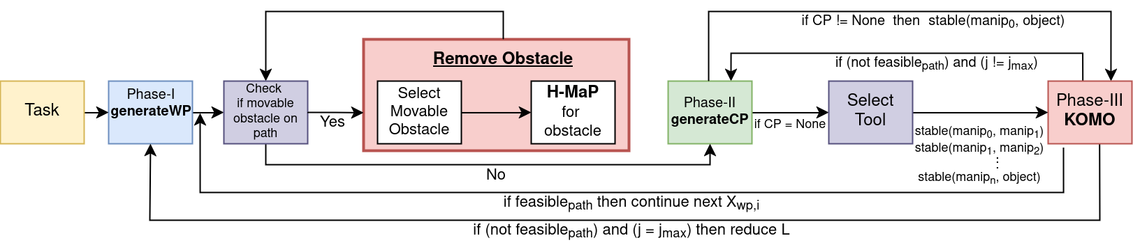
Figure 2: Flowchart for H-MaP with obstacle removal and tool selection stages. $\text{manipulator}_{0}$ is the end-effector by default, and $\text{manipulator}_{n}$ indicates the tool, where $n$ is the number of tools. Our experiments, which use a single tool ($n=1$), demonstrate that our approach is effectively focused on single-tool manipulations yet remains scalable to configurations involving multiple tools without loss of generality.

III PROBLEM STATEMENT

We first explain the k-order motion optimization formulation, called KOMO [11], that our approach builds upon. Subsequently, we introduce our problem formulation.

III-A Optimization Based Motion Planning with KOMO

KOMO focuses on optimizing robot trajectories through a general problem formulation that integrates constraints on movement. Therefore, it aims to find the most efficient path while complying with predefined physical and environmental constraints by solving the k-order non-linear optimization problem formulated in (1).

$$\min_{x_{0:T}} \sum_{t=0}^{T}f_{t}(x_{t-k:t})^{T}f_{t}(x_{t-k:t})$$ (1)

s.t. $$\forall t:g_{t}(x_{t-k:t})\leq 0,\quad h_{t}(x_{t-k:t})=0.$$

Here, $x_{t}\in\mathbb{R}^{n}$ denotes a configuration of robot and objects, while $x_{0:T}=(x_{0},\ldots,x_{T})$ represents a trajectory spanning a horizon $T$. The expression $x_{t-k:t}=(x_{t-k},\ldots,x_{t-1},x_{t})$ represents sequences of $k+1$ consecutive states, indicating the progression of states over time within the given framework. The functions $f_{t}(x_{t-k:t})$, $g_{t}(x_{t-k:t})$, and $h_{t}(x_{t-k:t})$, each mapping to $\mathbb{R}^{d_{t}}$, $\mathbb{R}^{m_{t}}$, and $\mathbb{R}^{l_{t}}$ respectively, are designed as arbitrary, first-order differentiable, non-linear, k-order, vector-valued functions. These functions serve to define cost metrics or set equality/inequality constraints for each timestep $t$.

III-B Problem Formulation

We consider the problem of prehensile and non-prehensile manipulation of rigid objects and tools with a robotic manipulator. For problem formulation, we adopt the KOMO framework with kinematic modes as outlined in [18], which leverages KOMO for motion optimization and incorporates kinematic switches for sequential manipulation.

We extend the problem formulation of [1, 29], by discretizing the path optimization. We optimize a path $x:[0,I]\rightarrow\mathcal{X}$ consisting of $I\in\mathbb{N}$ discrete states or waypoints. For each of the consecutive waypoints, we optimize a sub-path $x_{i}:[0,K_{i}T]\rightarrow\mathcal{X}_{i}$ consisting of $K_{i}\in\mathbb{N}$ phases or modes. Collection of each sub-paths, $\cup_{0}^{I}x_{i}$, gives the actual full path $x$.

We define the optimization problem for each segment path $x_{i}$ by employing $s_{k,i}$, which specifies the constraints and cost parameters for a particular phase $k_{i}$ along the path. A sequence of discrete variables $s_{1:K_{i}}$ is designated as a skeleton [18]. For each sub-path $x_{i}$, a different skeleton can be used. The configuration space, denoted as $\mathcal{X}$, spans both the $n$-dimensional joint space of the robot and the poses of $m$ rigid objects within $SE(3)^{m}$, starting from an initial configuration $x_{0}$ within $\mathcal{X}$.

Given a skeleton $s_{1:K,i}$, where $\forall_{i}\in[0,I]$, we solve the optimization problem

$$\min_{{x_{i}}:[0,K_{i}T]\rightarrow X} \int_{0}^{K_{i}T}f_{\text{path}}(\bar{x}_{i}(t),s_{k,i})\,dt+f_{\text{goal}}(x_{i}(T),s_{k,i})$$ (2a)

s.t. $$x_{i}(0)=x_{0,i},h_{\text{goal}}(x_{i}(T))=0,\,g_{\text{goal}}(x_{i}(T))\leq 0,$$ (2b)

$$\begin{aligned} \forall_{t}\in[0,T]:\quad&h_{\text{path}}(\bar{x}_{i}(t),s_{k,i}(t))=0,\\ &g_{\text{path}}(\bar{x}_{i}(t),s_{k,i}(t))\leq 0,\end{aligned}$$ (2c)

$$\begin{aligned} \forall_{k}\in\{1,...,K_{i}\}:\quad&h_{\text{switch}}(\hat{x}_{i}(t_{k}),s_{k-1,i},s_{k,i})=0,\\ &g_{\text{switch}}(\hat{x}_{i}(t_{k}),s_{k-1,i},s_{k,i})\leq 0,\end{aligned}$$ (2d)

Within this model, the path constraints, labeled as $(h,g)_{\text{path}}$, rely on the comprehensive state $\bar{x}(t)=(x(t),\dot{x}(t),\ddot{x}(t))$ to validate that the trajectory adheres to both physical laws and kinematic constraints, ensuring feasible motion paths. The cost function for the path, $f_{\text{path}}$, incorporates control efforts, specifically chosen as the sum of squared joint accelerations to evaluate and minimize the effort required for path execution. The terms $(f,h,g)_{\text{goal}}$ denote a variety of objectives or conditions that the final state of the system is required to achieve or satisfy, ensuring the fulfillment of specified end goals. Additionally, $f_{\text{goal}}$ incorporates the sum of squared distance between the manipulator and the contact point. The terms $(h,g)_{\text{switch}}$ specify the constraints that facilitate smooth transitions between different operational modes, $s_{k-1}$ and $s_{k}$, relying on the extended state $\hat{x}=(x,\dot{x})$ to ensure these transitions are both feasible and differentiable.

IV ITERATIVE HYBRID MANIPULATION PLANNER

The hybrid sequential manipulation planner (H-MaP) is composed of three essential phases: waypoint generation, contact point generation, and optimization-based motion planning phases (Fig. 2). A detailed explanation of each phase is given in subsequent sections. During the waypoint generation phase, we construct a sequence of intermediate steps, denoted as $\{X_{\textrm{wp}}\}$, for the target object, composing the series of poses that outline the movement path from the starting point ($X_{0}^{\text{obj}}$) to the desired endpoint ($X_{G}^{\text{obj}}$). This phase is essential as it offers a decomposition approach to the manipulation problem, thereby facilitating a breakdown of complex tasks.

In the second phase, we generate contact points which indicate the locations where the robot physically interacts with the target object, i.e., where the manipulator makes contact with the object. In H-MaP, by default, the manipulator ($ID_{\text{manip}}$) is selected as the robot’s end-effector, with exceptions made for tool-use scenarios where the tool becomes the manipulator (Fig. 2). We extend the contact sampling methodology described in [2] with perception and supervised learning by using point cloud-based and regression model-based sampling. This phase is essential since contact points inform the solver where the kinematic modes change, and this helps to prevent the optimization-based solver from trapping into local minima and provides computational efficiency.

Contact points are generated iteratively to inform the optimization-based solver KOMO [11]. This information is crucial, particularly when kinematic mode changes are required, such as re-configuring grasp locations. Subsequently, full motion plan is computed between two consecutive waypoints by the KOMO solver. In essence, three phases of H-MaP iterate until the path optimization is completed feasibly between entire consecutive waypoints (Alg. 1).

Inputs:

$X_{0}$ $\triangleright$ initial configuration

$X_{G}^{\text{obj}}$ $\triangleright$ goal pose of the selected object

$\tau$ $\triangleright$ threshold distance to goal pose

$path$ $\triangleright$ empty list to store paths

$L$ $\triangleright$ distance between nodes in interpolation

$\text{j}_{\textrm{max}}$ $\triangleright$ max. iteration count for inner loop

// Initialize path feasibility flag

$feasible_{\textrm{path}}\leftarrow\text{False}$

while $!\text{feasible}_{\textrm{path}}$ do

       // WP generation phase

       $X_{\textrm{wp}}\leftarrow\text{{ObjectBasedRRT}}(X_{0},X_{G}^{\text{obj}},L)$

       // $I$: number of waypoints, len($X_{\textrm{wp}}$)

       // Main Loop, initialized with i=0

       while $(\|X_{i}^{\text{obj}}-X_{G}^{\text{obj}}\|>\tau)\;\land\;(\text{i}\not=I)$ do

             $\text{j}\leftarrow 0$ $\triangleright$ reset iteration number of inner loop

             $feasible_{\textrm{path}}\leftarrow\text{False}$ $\triangleright$ re-initialize the flag

             while $(!\text{feasible}_{\textrm{path}})\land(\text{j}\not=\text{j}_{\textrm{max}})$ do

                  

                  // CP generation phase

                   // $ID_{\textrm{obj}}$: object of interest

                   // $ID_{\textrm{manip}}$: manipulator

                   $C$ $\leftarrow$ GenerateCP($X_{i},ID_{\textrm{obj}},ID_{\textrm{manip}}$)

                  

                  // Optimization phase-II

                  

                  // $X_{\textrm{wp},i}$: selected WP as sub-goal

                   $X_{i+1}$, path(i), $feasible_{\textrm{path}}$ $\leftarrow\text{{KOMO}}(X_{i}$, C, $ID_{\textrm{manip}},$ $X_{\textrm{wp},i}$)$)$

                   j $\leftarrow$ j + 1 $\triangleright$ increment number of iteration

            

            if $feasible_{\textrm{path}}$ then

                   // Append path(i) to the overall path

                   $path\leftarrow path\cup\{\text{path}(i)\}$

                   i $\leftarrow$ i + 1 $\triangleright$ increment counter

            else

                   $L\leftarrow L_{\textrm{new}}$ $\triangleright$ reduce $L$

                   break

            

      

return $path$

Algorithm 1 H-MaP Algorithm

IV-A Waypoint Generation

In this phase, the path extraction focuses solely on the target object ($ID_{\textrm{obj}}$) to simplify the problem by reducing the dimensionality of the configuration space. Consequently, the RRT [23] algorithm computes the path for the object by treating it as having full degrees of freedom in 3D space. During this step, interactions between the robot and the object are not accounted for. In effect, the path is first generated by RRT and then passed to the optimizer, ensuring probabilistic completeness from RRT and introducing both optimality and smoothness through the optimization process. Subsequently, an interpolation step is executed to extract waypoints, $X_{\textrm{wp}}$, as intermediate points along the trajectory. This step enhances discretization, improving the likelihood of finding a feasible path among the discretized waypoints in the final optimization phase of H-MaP. Furthermore, it enhances the computational efficiency of RRT by diminishing the necessity to reduce the RRT’s node extension distance parameter for discretization purposes.

Although the feasibility of H-MaP increases with a higher number of waypoints, its efficiency is adversely affected due to the increased number of optimization steps required. Therefore, the interpolation step, which increases waypoint numbers, induces a trade-off between computational efficiency and the feasibility of H-MaP. Hence, it is only utilized when H-MaP fails to produce a feasible path. The node distance (L), acting as an adjustable hyperparameter, is gradually reduced until H-MaP finds a feasible path, ensuring a balanced approach to achieving efficiency and effectiveness in pathfinding (Alg. 2).

Inputs:

$X_{0}$ $\triangleright$ initial configuration

$X_{G}^{\text{obj}}$ $\triangleright$ goal pose of the selected object

$X_{0}^{\text{obj}}$ $\triangleright$ initial pose of the selected object

$L$ $\triangleright$ distance between nodes in interpolation

// Object Based RRT phase

// Find List of Waypoints

while $path_{\textrm{sampled}}\not=Feasible$ do

       $path_{\textrm{sampled}}$ $\leftarrow$ RRT($X_{0}^{\text{obj}}$ , $X_{G}^{\text{obj}}$)

// optimize the path generated by RRT

$path_{\textrm{optimized}}$ $\leftarrow$ KOMO($path_{\textrm{sampled}}$)

// Interpolate the path to get WPs

$X_{\textrm{wp}}$ $\leftarrow$ InterpolateWPs($path_{\textrm{optimized}}$ , L)

return $X_{\textrm{wp}}$

Algorithm 2 ObjectBasedRRT

IV-B Contact Point Generation

We employ two distinct techniques for generating contact points. As the first method, we use a point cloud-based contact sampling approach. A point is randomly selected from the point cloud of the object, and its position is then transformed from global coordinates to the coordinate frame of the target object. This conversion facilitates the calculation of contact points in the context of the object’s coordinate frame rather than the global (world) frame, which is crucial for integrating contact point data into motion planning algorithms (Alg. 3).

The second technique for contact point generation employs neural network based regression models. Initially, we construct a regression model and annotate the dataset with labeled contact points. We create a dataset by randomizing object features for sample generation, followed by labeling with human-defined contact regions. This model is then trained using data from the configuration space alongside these labels, enabling it to infer contact points based on the configuration space, which includes the pose of the robot, objects, and obstacles within the environment. Integrating the regression model facilitates enhancements in acceleration and scalability through supervised learning, especially in the context of complex manipulation problems.

Inputs:

$X_{i}$ $\triangleright$ initial configuration

$ID_{\textrm{obj}}$ $\triangleright$ selected (target) object name

$ID_{\textrm{manip}}$ $\triangleright$ selected manipulator name

// CP generation phase

while $\text{result}_{\textrm{CP}}$ $\not=Feasible$ do

       // Extract point cloud

       $PointCloud$ $\leftarrow$ getCameraView($X_{i}$, $ID_{\textrm{obj}}$)

      

      // Sample contact point

       $C_{\textrm{global}}$ $\leftarrow$ findContactPoint(PointCloud)

      

      // Convert CP relative to target object

       $C$ $\leftarrow$ convertCPrelative($X_{i}$, $ID_{\textrm{obj}}$)

      

      // Optimization phase-I

       // Check the feasibility of contact

       $\text{result}_{\textrm{CP}}$ $\leftarrow$ KOMO($X_{i}$, C, $ID_{\textrm{manip}}$) $\triangleright$ IK solution

      

return C

Algorithm 3 GenerateCP (Sampling Based)

IV-C Optimization-Based Motion Planning

The optimization for the motion planning phase consists of two stages. In the first stage, Optimization phase-I (Alg. 3), optimization is used to check the feasibility of a contact point generated by the methods described in Sec. IV-B. A contact point is generated until the optimization solver identifies a valid configuration where the manipulator’s contact with the object is feasible. The first optimization problem is constructed in an inverse kinematic setting:

$$\min_{x_{T}} f_{T}(x_{T})^{T}f_{T}(x_{T})$$ (3)

s.t. $$g_{T}(x_{T})\leq 0,\quad h_{T}(x_{T})=0.$$

$h_{T}(x_{T})=|X_{\text{pos}}^{\text{manip}}(x_{T})-C_{\text{pos}}|=0$, enforces touch constraint. $C_{\text{pos}}$ indicates the position of the generated contact point. The feasibility of the final configuration $x_{T}$ is evaluated based on the constraint violation within the optimization process.

In Optimization phase-II, motion planning is done by optimization from the current state to a designated sub-goal to calculate $x_{i}$ as formulated in Eq. (3). Within this phase, we use pre-defined skeletons
(touch $\textit{ID}_{\textrm{manip}}$ $\textit{ID}_{\textrm{obj}}$) (stable $\textit{ID}_{\textrm{manip}}$ $\textit{ID}_{\textrm{obj}}$)
(poseEq $\textit{ID}_{\textrm{obj}}$ goal)
where each line corresponds to one phase step $s_{k}$, the predicate stable describes the mode switch, and touch and poseEq are geometric constraints. We use the same predicates defined as in [1]. The stable predicate makes a relative transformation constant between a manipulator and an object. This adds the object to the kinematic chain of the manipulator. The touch predicate enforces the distance between a manipulator and an object equal to zero. The poseEq predicate enforces that the object reaches a specific goal pose, $X_{\textrm{wp},i}$ in our case. In addition to these predicates, $|X_{\text{pos}}^{\text{manip}}-C_{\text{pos}}|$ added as a sum-of-square cost to Eq. (2a) to impose touch in proximity of generated contact point $C$.

After adding these constraints, we solve the optimization problem with KOMO solver. Then, we evaluate the feasibility of the action according to the constraint violation computed by the solver. If the action is feasible, we append the path to the path list, $x\cup x_{i}$, and continue to the next waypoint $X_{\textrm{wp},i+1}$. If the action is not feasible, the solver iterates until it finds a feasible action by generating a new contact point $C$ in the current waypoint $X_{\textrm{wp},i}$.

The proposed method employs a two-phase optimization strategy, initially addressing an inverse kinematics problem as a lower bound to efficiently find a feasible contact configuration before tackling the full problem. This prioritization improves overall computational efficiency by solving for the optimal final configuration first and only then proceeding to trajectory optimization towards a specific sub-goal $X_{wp,i+1}$.

V EXPERIMENTS & RESULTS

To evaluate our algorithm, we designed six different tasks with varying difficulties involving multiple contact mode changes, obstacles, tool-use and auxiliary objects. While designing the tasks, we were inspired by real-life manipulation problems. The experiments were done in the Rai simulator [30]. The Franka-Panda robot is used in simulation as well as in real-life experiments. Several RGBD cameras are included in the simulation for point cloud extraction, which is then utilized by the contact point generation algorithm. All object and obstacle models are available to the contact sampler algorithm. Due to the varying difficulty levels of each task, the time it takes to find a feasible solution varies. Finding a solution roughly takes a minute, but the time can be further reduced by using a regression-based method over a point cloud-based sampling method during the contact point generation phase. We illustrate this enhancement in the movable and non-movable obstacles tasks, and the approach is also adaptable to other tasks. To demonstrate robustness, our algorithm was evaluated multiple times on the same tasks, with modifications including size and pose variations of object and obstacle, as well as changes in goal pose. It successfully completed all tasks within a reasonable timeframe consistently (Table I).

Task	WP count	RRT (s)	CP (s)	KOMO (s)
Lock	36 $\pm$ 4	45 $\pm$ 8.4	18.6 $\pm$ 2.2	1.58 $\pm$ 0.3
Obs. Around	17 $\pm$ 3	1.8 $\pm$ 0.6	0.1* $\pm$ 0.0	0.9 $\pm$ 0.05
Obs. Move	12 $\pm$ 1	0.92 $\pm$ 0.1	0.1* $\pm$ 0.0	1.84 $\pm$ 0.3
Tunnel	24 $\pm$ 2	0.50 $\pm$ 0.1	29.8 $\pm$ 5.4	2.88 $\pm$ 0.6
Tunnel Tool	30 $\pm$ 1	0.76 $\pm$ 0.2	32.7 $\pm$ 1.9	12.4 $\pm$ 1.4
Bookshelf	37 $\pm$ 1	0.13 $\pm$ 0.01	11.8 $\pm$ 2.6	36.18 $\pm$ 4.34

TABLE I: Performance Metrics for Different Tasks. “WP count” represents the number of waypoints $I$; “RRT,” “CP,” and “KOMO” denote the time in seconds for waypoint generation, contact point generation, and optimization phases, respectively. Data are presented as “mean” ± “standard deviation” for ten runs of each task. * indicates that contact points are calculated using a supervised model.

V-A Results for Test Cases

The object through the tunnel (tunnel) task (Fig. 3-a) involves transferring a single object through a tunnel. The robot should push the object from one side and pick it up from the other side. The challenging aspect of this task is that the manipulator has to iteratively push the object without colliding with the tunnel until it can be pulled out of the other end. It cannot do this operation in one go and has to sample multiple contact points to follow the generated waypoints.

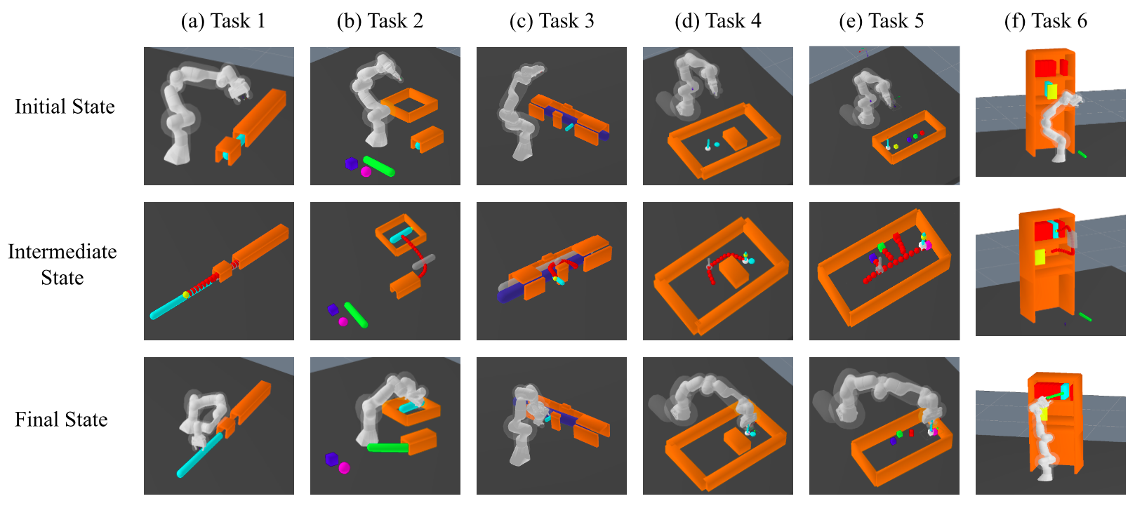
Figure 3: From left to right: object through the tunnel; object through the tunnel with a tool; sliding latch lock; pushing an object with a tool around a non-movable obstacle; and pushing an object with a tool while removing movable obstacles. The top and bottom rows indicate the initial and final configurations, respectively. The middle row includes generated waypoints (red spheres), contact points (yellow spheres), and the intermediate state of the object (gray silhouette) during the task.

The object through the tunnel with a tool (tunnel with tools) task (Fig. 3-b) is similar to the tunnel task, but in this task, the object is unreachable by the robot since it is entirely under the tunnel. The robotic manipulator must interact with the nearby tools by selecting the feasible one and pushing the object from under the tunnel until the robot can directly manipulate it. Then, the robotic arm has to grab the accessible object and put it inside the nearby box. This case is significantly more complicated than the previous task since it requires tool use in addition to contact point sampling and manipulation planning.

The sliding latch lock (lock opening) task (Fig. 3-c) requires the Panda robotic arm to interact with the lock handle, aiming to unlock it through movements along the vertical and horizontal axes. This task is challenging for optimization-based planning algorithms since they tend to get stuck in local minima due to the nonlinear constraints induced by the obstacles. Waypoint generation is relatively harder as well, due to the necessity of non-trivial rotational movement of the object in a highly constrained environment (Table I).

Pushing an object with a tool around a non-movable obstacle (non-movable obstacle) task (Fig. 3-d) demonstrates the capability of the algorithm to navigate through obstacles while interacting with an object. The goal is to push the object, by using the tool, to the desired goal position without colliding with the obstacles in its path. The solution is not trivial since it requires pushing the object from different contact points.

Pushing an object with a tool while removing movable obstacles (movable obstacles) task (Fig. 3-e) simulates an environment where it requires tool use and obstacle manipulation. The robotic arm is supposed to pick the tool and push the target object to the desired position. However, since the waypoint generation phase does not take into account (movable) objects other than the target, some objects might block the path generated by the object-based RRT. The manipulator should push such obstacles out of the object’s path by using the tool. The complexity of this task is the requirement of interaction with multiple objects to generate a feasible path for the desired object.

Pick and place a book in a bookshelf (bookshelf) task (Fig. 3-f) task entails the removal of an obstacle blocking the book and subsequently placing the book on an upper shelf, followed by using a tool to push it into alignment with other books. This task presents a notable challenge, as identifying a feasible contact mode for the robot to grasp the book post-obstacle removal is complex. Feasible contact points are limited primarily to the middle region of the book, with other points leading to local minima that preclude viable contact modes. Another significant challenge is charting a feasible path without trapping into local minima to transport the book from a lower position to the upper shelf. These challenges emphasize the complexity of the task when not addressed through a combined strategy of waypoints and contact point resolution.

Real robot experiments (Fig .1 and Fig. 4): To validate our method, we conducted experiments for the movable obstacles and non-movable obstacles tasks using a Franka Panda robot. The planning was performed in simulation and then transferred to the actual robot. Although a controller could be employed for robust operation, our experiments were successfully managed with open-loop execution.

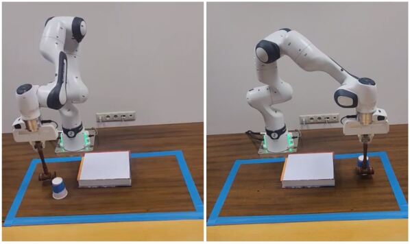
Figure 4: Real Robot Experiment. Pushing an object with a tool around a non-movable obstacle. Initial (left) and goal (right) states.

V-B High-Level Comparison with Baseline Methods

In this section, we discuss and compare our method w.r.t.  two baseline methods: LGP [18] and dexterous manipulation solvers [2, 3]. First, since LGP uses KOMO for motion optimization, it still has the risk of trapping into local minima. Therefore, LGP, provided with pick, place and push primitives, fails in latch, non-movable obstacle and bookshelf tasks. In these tasks, the solver can only provide an “infeasible” path that violates the collision constraint. Second, due to local minima, switching contact points on the same object turns out to be problematic in LGP. For instance, LGP struggles to find a solution in a reasonable time in tunnel and tunnel with tool tasks. However, since it does not involve a constraint environment, it could solve the movable obstacles task.

Dexterous manipulation solvers [2, 3] are good at dynamically changing contact modes by using their sampling approaches. Therefore, they could handle the tunnel and latch tasks without trapping into local minima. Despite this, an attempt to resolve the latch task using RRT failed to yield a feasible solution in a reasonable time compared to object-based RRT, likely due to the highly constrained nature of the problem. Even though tool-use and ancillary object manipulation are not within the scope of these studies, it is also not trivial to integrate such skills. The configuration space excessively expands in tunnel with tool, movable obstacles, non-movable obstacle, and bookshelf tasks. This makes these tasks significantly challenging to solve by these methods since they consider the whole task as a single motion planning problem.

Despite the challenges in achieving complex manipulation with optimization-based sequential planning, H-MaP overcomes these by generating sub-goals through object-based RRT, minimizing the reliance on predefined action primitives. This approach enables handling complex sequential manipulation tasks that involve both active kinematic mode switches and auxiliary object manipulation cases.

V-C Scalability of H-MaP: Towards Task-Level Reasoning

The scalability of H-MaP hinges on the abstraction of actions into primitives and kinematic modes, facilitating diverse action creation through predicates as outlined in Section IV-C. Furthermore, the modular design of H-MaP adapts to various scenarios, including tool-use in tasks where direct manipulation is infeasible, by utilizing a tool selection stage (Fig. 2). For instance, in tunnel with tools task, contact point generation, and tool selection stages enable the creation of the following conditional stages: “If the end-effector cannot manipulate the object, then manipulate it with auxiliary objects (treated as manipulators) in the environment” and “Move the object with the manipulator until it becomes pickable.” Additionally, obstacle removing stage allows for dynamic problem-solving, extending its application to manipulate ancillary objects, as demonstrated in the movable obstacles task. Integration of high-level task planning using search-based methods can enable H-MaP to automate the creation of complex action sequences. These functionalities pave the way for an integrated TAMP solver that can plan and execute complex manipulations with task-level reasoning.

V-D Limitations

Our solver demonstrates promising results; however, it is not without its limitations:

Transition between waypoints: At present, our solver does not consider transitions directly from $X_{\textrm{wp},i}$ to $X_{\textrm{wp},i+2}$. This oversight may limit its capacity to identify feasible paths in scenarios where moving from $X_{\textrm{wp},i+1}$ to $X_{\textrm{wp},i+2}$ is impractical, yet a direct path from $X_{\textrm{wp},i}$ to $X_{\textrm{wp},i+2}$ is possible. Although this situation has not occurred in our experiments, implementing backtracking methods could improve the solver by addressing this limitation.

Assumption on waypoint quality: The solver operates under the assumption that all waypoints generated via the RRT algorithm are viable. If the waypoints are poorly generated, the solver may fail to find a solution. To alleviate this problem, we regenerate RRT-based waypoints if no feasible path is found.

Kinematic systems focus: The current version of our solver focuses exclusively on kinematic systems. While this allows for a simplified model that is easier to analyze and optimize, it neglects the dynamics of the system, which is crucial for a more comprehensive understanding and application. To enhance the accuracy and applicability of our approach for real-world settings, dynamics-related features can be integrated for planning, along with a controller for execution.

VI CONCLUSION and DISCUSSION

Unlike prior methods that apply RRT to both the robot and the object, considering their kinematic states, our approach specifically targets the path calculation for the target object. This focus significantly reduces the dimensionality of the configuration space, offering a substantial advantage for complex sequential manipulation planning. Moreover, most current manipulation planning methods are limited to interactions between a single robot and an object, neglecting the interaction with ancillary objects such as movable obstacles or tools. Our method addresses this limitation; enhancing the robot’s ability to perform complicated tasks requiring tool-use and ancillary object manipulation.

Results demonstrate that enhancing “low-level” motion planners for sequential manipulation tasks eliminates the need for explicitly defined motion primitives for each action. This method reduces the necessity to pre-define “high-level” actions, allowing the solver to execute such actions implicitly. For instance, in the task of lock opening, it eliminates the requirement to specify additional discrete actions such as lift up, pull left, and pull down. Consequently, it streamlines the planning process by enabling more intuitive and flexible problem-solving approaches.

In essence, this study makes a step towards manipulation planning for complex reasoning tasks, establishing a foundation for advanced, long-horizon manipulation planning strategies. For future developments, we aim to augment our solver with integrated task and motion planning capabilities, targeting more complex and dexterous manipulation tasks. Additionally, we aim to refine our methodologies for generating contact points and waypoints, further increasing the efficiency and effectiveness of our system in complex environments.

References

- [1] M. A. Toussaint, K. R. Allen, K. A. Smith, and J. B. Tenenbaum, “Differentiable physics and stable modes for tool-use and manipulation planning,” Proceedings of the Robotics: Science and Systems Foundation, 2018.
- [2] T. Pang, H. T. Suh, L. Yang, and R. Tedrake, “Global planning for contact-rich manipulation via local smoothing of quasi-dynamic contact models,” IEEE Transactions on Robotics, vol. 39, no. 6, pp. 4691–4711, 2023.
- [3] X. Cheng, E. Huang, Y. Hou, and M. T. Mason, “Contact mode guided motion planning for quasidynamic dexterous manipulation in 3d,” in IEEE International Conference on Robotics and Automation (ICRA), pp. 2730–2736, 2022.
- [4] G. Lee, T. Lozano-Perez, and L. P. Kaelbling, “Hierarchical planning for multi-contact non-prehensile manipulation,” IEEE/RSJ International Conference on Intelligent Robots and Systems (IROS), pp. 264–271, 2015.
- [5] D. E. McCoy, M. Schiestl, P. Neilands, R. Hassall, R. D. Gray, and A. H. Taylor, “New caledonian crows behave optimistically after using tools,” Current Biology, vol. 29, no. 16, pp. 2737–2742, 2019.
- [6] Wikipedia contributors, “Latch.” https://en.wikipedia.org/wiki/Latch, 2024. Last visited on 2024-02-18.
- [7] D. M. Wolpert and J. R. Flanagan, “Motor prediction,” Current biology, vol. 11, no. 18, pp. R729–R732, 2001.
- [8] M. Kawato, “Internal models for motor control and trajectory planning,” Current opinion in neurobiology, vol. 9, no. 6, pp. 718–727, 1999.
- [9] F. Osiurak and A. Badets, “Tool use and affordance: Manipulation-based versus reasoning-based approaches.,” Psychological review, vol. 123, no. 5, p. 534, 2016.
- [10] U. Kleinholdermann, V. H. Franz, and K. R. Gegenfurtner, “Human grasp point selection,” Journal of vision, vol. 13, no. 8, pp. 23–23, 2013.
- [11] M. Toussaint, “Newton methods for k-order markov constrained motion problems,” arXiv preprint arXiv:1407.0414, 2014.
- [12] M. Toussaint, “A tutorial on newton methods for constrained trajectory optimization and relations to slam, gaussian process smoothing, optimal control, and probabilistic inference,” Geometric and numerical foundations of movements, pp. 361–392, 2017.
- [13] M. Zucker, N. Ratliff, A. D. Dragan, M. Pivtoraiko, M. Klingensmith, C. M. Dellin, J. A. Bagnell, and S. S. Srinivasa, “Chomp: Covariant hamiltonian optimization for motion planning,” The International journal of robotics research, vol. 32, no. 9-10, pp. 1164–1193, 2013.
- [14] A. D. Dragan, N. D. Ratliff, and S. S. Srinivasa, “Manipulation planning with goal sets using constrained trajectory optimization,” in IEEE International Conference on Robotics and Automation (ICRA), pp. 4582–4588, 2011.
- [15] A. D. Dragan, G. J. Gordon, and S. S. Srinivasa, “Learning from experience in manipulation planning: Setting the right goals,” in Robotics Research: The 15th International Symposium ISRR, pp. 309–326, Springer, 2017.
- [16] M. Kalakrishnan, S. Chitta, E. Theodorou, P. Pastor, and S. Schaal, “Stomp: Stochastic trajectory optimization for motion planning,” in IEEE International Conference on Robotics and Automation (ICRA), pp. 4569–4574, 2011.
- [17] J. Schulman, Y. Duan, J. Ho, A. Lee, I. Awwal, H. Bradlow, J. Pan, S. Patil, K. Goldberg, and P. Abbeel, “Motion planning with sequential convex optimization and convex collision checking,” The International Journal of Robotics Research, vol. 33, no. 9, pp. 1251–1270, 2014.
- [18] M. Toussaint, “Logic-geometric programming: An optimization-based approach to combined task and motion planning.,” in IJCAI, pp. 1930–1936, 2015.
- [19] D. Berenson, S. S. Srinivasa, D. Ferguson, and J. J. Kuffner, “Manipulation planning on constraint manifolds,” in IEEE International Conference on Robotics and Automation (ICRA), pp. 625–632, 2009.
- [20] Z. Kingston, M. Moll, and L. E. Kavraki, “Exploring implicit spaces for constrained sampling-based planning,” The International Journal of Robotics Research, vol. 38, no. 10-11, pp. 1151–1178, 2019.
- [21] P. S. Schmitt, W. Neubauer, W. Feiten, K. M. Wurm, G. V. Wichert, and W. Burgard, “Optimal, sampling-based manipulation planning,” in IEEE International Conference on Robotics and Automation (ICRA), pp. 3426–3432, 2017.
- [22] Y. C. Nakamura, D. M. Troniak, A. Rodriguez, M. T. Mason, and N. S. Pollard, “The complexities of grasping in the wild,” in IEEE-RAS 17th International Conference on Humanoid Robotics (Humanoids), pp. 233–240, 2017.
- [23] S. M. LaValle, “Rapidly-exploring random trees: A new tool for path planning,” tech. rep., Computer Science Department, Iowa State University, Ames, IA, USA, 1998.
- [24] C. R. Garrett, R. Chitnis, R. Holladay, B. Kim, T. Silver, L. P. Kaelbling, and T. Lozano-Pérez, “Integrated task and motion planning,” Annual review of control, robotics, and autonomous systems, vol. 4, pp. 265–293, 2021.
- [25] S. Cambon, R. Alami, and F. Gravot, “A hybrid approach to intricate motion, manipulation and task planning,” The International Journal of Robotics Research, vol. 28, no. 1, pp. 104–126, 2009.
- [26] O. Kroemer and J. Peters, “A flexible hybrid framework for modeling complex manipulation tasks,” in IEEE International Conference on Robotics and Automation (ICRA), pp. 1856–1861, 2011.
- [27] R. Alur, T. A. Henzinger, G. Lafferriere, and G. J. Pappas, “Discrete abstractions of hybrid systems,” Proceedings of the IEEE, vol. 88, no. 7, pp. 971–984, 2000.
- [28] J. Z. Woodruff and K. M. Lynch, “Planning and control for dynamic, nonprehensile, and hybrid manipulation tasks,” in IEEE International Conference on Robotics and Automation (ICRA), pp. 4066–4073, 2017.
- [29] M. Toussaint, J.-S. Ha, and D. Driess, “Describing physics for physical reasoning: Force-based sequential manipulation planning,” IEEE Robotics and Automation Letters, vol. 5, no. 4, pp. 6209–6216, 2020.
- [30] M. Toussaint, “Robotic systems toolbox.” GitHub repository, 2024. Available: https://github.com/MarcToussaint/robotic.