Model free collision aggregation for the computation of escape distributions

Abstract

Motivated by a heat radiative transport equation, we consider a particle undergoing collisions in a space-time domain and propose a method to sample its escape time, space and direction from the domain. The first step of the procedure is an estimation of how many elementary collisions is safe to take before chances of exiting the domain are too high; then these collisions are aggregated into a single movement. The method does not use any model nor any particular regime of parameters. We give theoretical results both under the normal approximation and without it and test the method on some benchmarks from the literature. The results confirm the theoretical predictions and show that the proposal is an efficient method to sample the escape distribution of the particle.

Keywords : heat radiative transfer equation; Monte Carlo simulation; collision transport equations

1 Introduction

Particle simulations offering insights into complex chemical systems at the molecular level and can help elucidate reaction mechanisms, predict thermodynamic properties, and explore molecular assembly; such methods have been successfully applied in various fields such as catalysis [1], atmospheric modelling [2, 3], radiation transport [8], etc. We will focus on the integro-differential transport equation :

$$\frac{1}{c}\partial_{t}u(t,x,\omega)+\omega\cdot\nabla u(t,x,\omega)+(\sigma_{a}(t,x)+\sigma_{s}(t,x))u(t,x,\omega)=\sigma_{s}(t,x)\langle{u}\rangle(t,x),$$ (1)

with time variable $t\in[0,T]$, position variable $x\in\mathcal{\mathcal{X}}\subset\mathbb{R}^{d}$ (here $d\geq 1$ is the spatial dimension), the angle of propagation $\omega\in\mathcal{S}^{d}$ (unit sphere in $\mathbb{R}^{d}$) and $\langle{u}\rangle(t,x)=\frac{\int_{\mathcal{S}^{d}}u(t,x,\omega^{\prime})d\omega^{\prime}}{\int_{\mathcal{S}^{d}}1\cdot d\omega^{\prime}}$ the angular average of $u$ on $\mathcal{S}^{d}$. The model represents heat radiative transfer equations that can be used for both photons and neutrons (we use the former in the numerical results).

The model also comes with a speed constant ; for instance for photons this will be the speed of light. The absorption opacity $\sigma_{a}$ and the scattering opacity $\sigma_{s}$ are (known) functions of $x$ and $t$ that describe the collision dynamics of the particles and more precisely the time to next collision, see section 2.1 for details.

The spatial domain $\mathcal{X}$ is usually a mesh simulation cell and various approximations are invoked to compute relevant quantities and manage the transition of particles from one mesh cell to another. We will not discuss this but refer to [4, 5] and related literature. The main focus of this paper will be on how to compute the evolution of one particle from the initial time $t_{0}=0$ and initial position $x_{0}\in\mathcal{X}$ to the moment when it exits the domain $\mathcal{X}\times[0,T]$, i.e. either reaches the spatial boundary $\partial\mathcal{X}$ or consumes all available time $T$.

We are concerned here with ’Monte Carlo’ approaches that regard (1) as the time-evolving probability density of a stochastic process, see [6]. When parameter $\sigma_{s}$ is large, many collisions occur before final time $T$ because the average time to next collision is $\frac{1}{\sigma_{s}}$. This is the so-called ’diffusion regime’ [7] and approximation methods exist to exploit this remark, in particular the Random Walk (RW) methods [8, 9]. On the contrary, when $\sigma_{s}$ is small, the particle will not undergo many collisions before exiting the mesh cell and the ballistic regime is important. In between, there are situations where the diffusion limit is not valid but the number of collisions is still important and requires extensive numerical simulations. Like in the diffusion limit, one would like to somehow accelerate this computation by replacing a large sum of independent collisions with some aggregate step, without resorting to diffusive approximations. So we focus in this paper on a model free method to aggregate many collisions into a single displacement without affecting the escape distribution of the particle. The simulation of the particle’s trajectory stops when either time ends (at $t=T$) or the particle reaches the spatial boundary $\partial\mathcal{X}$. Note that a single aggregated step will probably not suffice to end the simulation for the particle so several such movements will probably be used.

As a technical circumstance, we will invoke the discrete ordinate method, denoted $S_{N}$, which consists in discretizing the the angular direction variable i.e., replacing $\mathcal{S}^{d}$ by a set of discrete directions $\mathcal{D}$.

The outline of the paper is the following: we describe the collision dynamics of one particle in section 2.1. Then in section 2.2 we describe the general principle of the proposed method; in sections 2.3 and 2.4 we give several theoretical results. The procedure is then tested in section 3.

2 Procedure and associated theoretical insights

2.1 Description of the collision dynamics

We present briefly the dynamical setting. For graphical convenience this problem is presented in 1D but it transcribes without difficulty to the multi-dimensional case.

For further simplification we will restrict to a situation where the direction of the particle is either $+1$ or $-1$; this is the so-called $S_{2}$ discrete-ordinates method (see [10, section 16.3 page 502], which relates to the Schuster-Schwarzschild equations [10, section 14.3 p 456]. We will denote $\mathcal{D}_{2}=\{-1,1\}$ and in general

$$\mathcal{D}_{N}=\left\{cos\left(\frac{2\pi j}{N}\right),j=0,...,N-1\right\}.$$ (2)

Note that, for dimensions $d$ higher than $1$, the direction of the particle is an element of the unit sphere $\mathcal{S}^{d}$. We consider a $1D$ particle in the spacial domain $\mathcal{X}:=[0,L]$ starting from $x(0)=x_{0}\in\mathcal{X}$ at $t_{0}=0$. We are also given a maximum time $T$. The particles evolves as follows : the collision counter is set to $s=1$ and a direction $a_{s}\in\mathcal{D}$ is chosen at random uniformly from $\mathcal{D}$. A time $\tau_{s}$ is sampled from an exponential law of mean $1/\sigma$ (this will be denoted $\tau_{s}\sim Exp(\sigma)$). We define $t_{s}=t_{s-1}+\tau_{s}$. The particle moves on a straight line in the direction $a_{s}$ during the time $\tau_{s}$ at constant speed $v$. Thus for any $t\in[t_{s-1},t_{s}]$ : $x(t)=x(t_{s-1})+v(t-t_{s-1})a_{s}$.

Next, the collision counter $s$ is incremented $s\to s+1$ and the process repeats until either $t_{s^{\star}}\geq T$ or $x_{t_{s^{\star}}}\notin\mathcal{X}$. The precise space-time coordinates when the particle touches the first time the boundary of the domain $\mathcal{X}\times[0,T]$ are computed, i.e., for our simple 1D case the smallest $t^{\star}\in[t_{{s^{\star}}-1},t_{s^{\star}}]$ such that $x(t^{\star})=0$ or $x(t^{\star})=L$ or $t^{\star}=T$.

The quantity of interest is the distribution of the escape space-time, more precisely the joint distribution of the escape position $x^{\star}:=x(t^{\star})$, escape direction $a^{\star}\in\mathcal{D}$ and escape time $t^{\star}$ when the boundary is reached. This triplet $(x^{\star},t^{\star},a^{\star})$ is a random variable whose distribution $\mathcal{E}(\sigma,\mathcal{X},T,x_{0})$ depends only on $\mathcal{X}$, $\sigma$, $T$ and $x_{0}$.

An illustration is given in figure 1 for $\mathcal{D}=\mathcal{D}_{2}$. Note that the escape space-times values are elements of $\mathbb{R}^{2dim(\mathcal{X})+1}=\mathbb{R}^{3}$ thus the support of the distribution $\mathcal{E}(\sigma,\mathcal{X},T,x_{0})$ is formally included in $R^{3}$; but there are many restrictions on this support, for instance $t\in[0,T]$ and so on, leaving the support to be included in (see figure 1 for notations) :

$$\Big{(}AB\times\{-1\}\Big{)}\bigcup\Big{(}BC\times\{-1,1\}\Big{)}\bigcup\Big{(}CD\times\{1\}\Big{)}.$$ (3)

For instance, the explanation of the first element $AB\times\{-1\}$ is that if the particle exists through its left border the exit direction will point to the left. Or in $\mathcal{D}$ there is only one direction that points to the left which is $-1$; same for $CD\times\{1\}$.

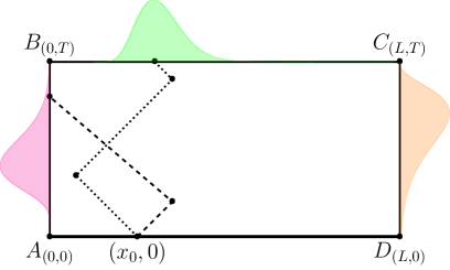
Figure 1: An illustration of the time dynamics and escape space-time distribution for a particle starting at $x_{0}$, $\mathcal{D}=\mathcal{D}_{2}$. The time to next collision is an exponential random variable of average $1/\sigma$ i.e. distributed $exp(\sigma)$. The joint escape distribution $\mathcal{E}(\sigma,\mathcal{X},T,x_{0})$ collects the location $x^{\star}$, time $t^{\star}$ and direction $a^{\star}$ when the boundary $x=0$, $x=L$ or $t=T$ is reached for the first time (i.e., particle hits $AB$, $BC$ or $CD$). The simulation is stopped when this happens.

The colored areas in figure 1 are a general illustration, not corresponding to any specific parameters, of the following three conditional distributions:

- the left area (magenta in color figure) is the distribution of the escape time $t^{\star}$ at which $x(t^{\star})=0$, conditioned by the fact that the particle touched $x=0$ before $T$ and before touching $x=L$ ;

- the top area (green in color figure) is the distribution of the escape position $x(t^{\star})$ conditioned by escaping because time $T$ was reached before reaching $x=0$ or $x=L$, i.e. $t^{\star}=T$,

- the right area (orange in color figure) is the equivalent to the magenta area when border is first reached for $x=L$.

2.2 Idea and first estimations

The dynamics described in section 2.1 is used to sample from the distribution $\mathcal{E}$. In particular the intermediate values are not useful and not used. We can thus imagine a way to accelerate the computation by ”skipping” these intermediary steps. For instance, when the diffusion parameter $\sigma$ is very large many collisions will occur before particle exits the space-time domain and in this case a random walk approximation could be valid. We do not want to use this kind of approximation here but remain as close as possible to the collisional dynamics.

Recall that the collision time $t_{n}$ is the sum of i.i.d $Exp(\sigma)$ random variables $\tau_{j}$ : $t_{n}=\sum_{j=1}^{n}\tau_{j}$; the law of $t_{n}$ is a Gamma distribution of parameters $n$ and $\sigma$.

The position $X_{n}=x(t_{n})$ is such that $X_{n}=x_{0}+\sum_{j=1}^{n}va_{j}\tau_{j}$, its law is a mixture of sums of two Gamma distributed random variables (one for each value in $\mathcal{D}$); we will make this precise latter. In any case we will show that for any $n$ one can sample directly and exactly from the joint law $(X_{n},t_{n})$. In this way we can advance the time by $t_{n}$ units and replace $n$ individual collisions by only one sample from this joint law.

But the question that arises is the following: what is the value of $n$ such that, with high certainty, we can make $n$ steps without exiting the space-time domain $\mathcal{X}\times[0,T]$ ? We look for a value of $n$ as large as possible such that, given some tolerance $\epsilon>0$ :

$$\mathbb{P}[\{\exists t\leq t_{n}:x(t)\notin\mathcal{X}\}\cup\{t_{n}\geq T\}]\leq\epsilon.$$ (4)

2.3 Estimates for $t_{n}$

2.3.1 Normal approximation for $t_{n}$

The first approach is to use a normal (Gaussian) approximation. For instance we know that $t_{n}$ has mean $n/\sigma$ and variance $n/\sigma^{2}$. For very large values of $n$, the $t_{n}$ will behave as a normal variable with same mean and variance, i.e. $\frac{\sigma}{\sqrt{n}}(t_{n}-n/\sigma)$ is ”close” to a standard normal. So, we will write $\mathbb{P}[t_{n}\geq T]\leq\epsilon$ is the same as $\mathbb{P}[\frac{\sigma}{\sqrt{n}}(t_{n}-n/\sigma)\geq\frac{\sigma}{\sqrt{n}}(T-n/\sigma)]\leq\epsilon$ which, if the normal approximation holds, will be true when $\frac{\sigma}{\sqrt{n}}(T-n/\sigma)]$ is larger than the $1-\epsilon$ quantile of the normal distribution. To simplify things we take as small error $\epsilon=1/1013594692=9.865876448374298e-10<1e-9$ corresponding to exactly 6 standard deviations. In this case, with high probability, $t_{n}$ will not be larger than $T$ if $\frac{\sigma}{\sqrt{n}}(T-n/\sigma)>6$ or, equivalently, $n+6\sqrt{n}\leq\sigma T$. So the aggregation rule becomes :

$$n\leq T\sigma+18-6\sqrt{T\sigma+9}.$$ (5)

Note that here $T\sigma$ is the mean number of collisions left till reaching the final time $T$ (each collision ”consumes” in average $1/\sigma$ time units).

2.3.2 Exact tail approximation for $t_{n}$

We can also give a more precise, but slightly less convenient, estimation for $n$ coming from the tail estimates for the gamma distribution.

Proposition 1.

With previous notations, choosing $n\leq T\sigma/2$:

$$\mathbb{P}[t_{n}\geq T]\leq\frac{z^{z/2}e^{-z}}{\Gamma(1+z/2)},\text{ where }z=T\sigma.$$ (6)

In particular :

$$\mathbb{P}[t_{n}\geq T]\leq 10^{-9},\text{ if }n\leq T\sigma/2,n\geq 50.$$ (7)

Proof.

We are interested in $\mathbb{P}[t_{n}\geq T]=\mathbb{P}[\sigma t_{n}\geq T\sigma]$. Note that $\sigma t_{n}$ is a gamma random variable with parameters shape=$n$ and scale=$1$ and density $f(y)=\frac{1}{(n-1)!}y^{n-1}e^{-y}$. We need to give a bound for $\mathbb{P}[\sigma t_{n}\geq T\sigma]=\int_{T\sigma}^{\infty}\frac{1}{(n-1)!}y^{n-1}e^{-y}dy$. By integration by parts for general $z>0$ :

$$\int_{z}^{\infty}\frac{y^{n-1}}{(n-1)!}e^{-y}dy=\frac{y^{n}}{n!}e^{-y}\Big{|}_{y=z}^{\infty}+\int_{z}^{\infty}\frac{y^{n}}{n!}e^{-y}dy\geq\frac{z}{n}\int_{z}^{\infty}\frac{y^{n-1}}{(n-1)!}e^{-y}dy-\frac{z^{n}}{n!}e^{-z}.$$ (8)

Reordering the terms it follows that, for $z>n$ :

$$\int_{z}^{\infty}\frac{y^{n-1}}{(n-1)!}e^{-y}dy\leq\frac{nz^{n}e^{-z}}{n!(z-n)}=\frac{nz^{n}e^{-z}}{\Gamma(n+1)(z-n)}.$$ (9)

Let us take now $n=z/2$; the right hand side equals $\frac{z^{z/2}e^{-z}}{\Gamma(1+z/2)}$. The function $z\mapsto\ln\left(\frac{z^{z/2}e^{-z}}{\Gamma(1+z/2)}\right)=\frac{z}{2}\ln(z)-z-\ln(\Gamma(1+z/2))$ has derivative $\frac{\ln(z)-1}{2}-\psi(1+z/2)=\frac{\ln(z)-1}{2}-\frac{2}{z}-\psi(z/2)\leq\frac{\ln(z)-1}{2}-\frac{2}{z}-\ln(z)=\frac{1}{2}\ln(\frac{4}{ze})\leq 0$ as soon as $z\geq 2$; we have used the notation for the digamma function $\psi(z)=\frac{\Gamma^{\prime}(z)}{\Gamma(z)}$, relation $\psi(z+1)=\psi(z)+1/z$ and the inequality $\ln(z)-\frac{1}{z}\leq\psi(z)$ for all $z>0$. This shows that the error term $\frac{z^{z/2}e^{-z}}{\Gamma(1+z/2)}$ is decreasing for $z\geq 2$. In particular its value at $z=100$ is $2.44\times 10^{-10}<10^{-9}$. Conclusion (7) follows because $n\mapsto\mathbb{P}[t_{n}\geq T]$ is obviously increasing with $n$ and the value at $n=T\sigma/2$ is less than $10^{-9}$. ∎

2.3.3 Summary for $t_{n}$

To summarize, in order to satisfy $\mathbb{P}[t_{n}\geq T]<10^{-9}$ we have two possible choices

• the rigorous, conservative estimate from (7) with choice $n\leq T\sigma/2$ as soon as $n\geq 50$

• the normal approximation (5) resulting in the bound : $n\leq T\sigma+18-6\sqrt{T\sigma+9}$. In practice we require $n$ to be larger than some $n_{\mathcal{N}}$ that we set to $n_{\mathcal{N}}:=300$ in order to ensure that the normal approximation is in the asymptotic regime.

The normal approximation provides larger (thus less restrictive) values for $n$ but its quality is not precisely quantified. On the other hand, the conservative estimate (7) has a known error bound and works even if only one hundred average collisions are left in the time interval. If no other parameters enter into the decision, the number of such ”aggregated collisions” required to reach final time $T$ is $O(1)$ for the normal approximation and $O(\log(T\sigma))$ for the conservative estimate (each step halves the time ”left”). Both give very good results for the numerical regimes we are interested in.

2.4 Estimates for the spatial boundary

We now inquire about estimating the number of collisions that can be aggregated without reaching the spatial boundary. Define $D$ to be the distance from $x_{0}$ to the boundary of $\mathcal{X}$ i.e., $D=\min\{x_{0},L-x_{0}\}$. In general, if the spatial domain is $\mathcal{X}$ we set $D=dist(x_{0},\partial\mathcal{X})$. Note that $E[X_{n}-x_{0}]=0$, $\mathbb{V}[X_{n}-x_{0}]=nv^{2}/\sigma^{2}$. But, this still does not tell us if some other $X_{k}$ for $k\leq n$ did not already exited through the spatial domain boundaries $\{0\}$ or $\{L\}$. We can write :

$$\mathbb{P}[\{\exists t\leq t_{n}:x(t)\notin\mathcal{X}\}]\leq\mathbb{P}[\{\max_{s\leq t}|X_{s}-x_{0}|\geq D\}]=\mathbb{P}[\{\max_{s\leq t}|\sum_{j=1}^{s}a_{j}\tau_{j}|\geq D/v\}].$$ (10)

2.5 Spatial boundary treatment, no Gaussian approximation

We will consider a general case when $\mathcal{D}$ is not necessary $\{-1,1\}$. We will assume :

$$\text{Hypothesis on directions (HD)}~{}:\forall j\geq 0~{}:\mathbb{E}[a_{j}]=0,\mathbb{V}[a_{j}]=\varsigma^{2},\ a_{j}\text{ is symmetric}.$$ (11)

In practice this can restrict for instance the number of directions to be even for the $S_{N}$ model (to ensure symmetry). Note that for $\mathcal{D}=\mathcal{D}_{N}$ : $\varsigma=\sqrt{N/2}$. We will need the following result.

Proposition 2.

Consider $Y_{n}=\sum_{j=1}^{n}Z_{j}$ with $Z_{j}$ symmetric i.i.d. variables such that for some $\lambda>0$ : $\mathbb{E}[e^{\lambda Z_{1}}]<\infty$. Then for any $C\geq 0$

$$\mathbb{P}[\max_{j\leq n}|Y_{j}|\geq C]\leq 4\mathbb{P}[Y_{n}\geq C]=2\mathbb{P}[|Y_{n}|\geq C]$$ (12)

$$\mathbb{P}[\max_{j\leq n}|Y_{j}|\geq C]\leq 2e^{-\lambda C}\left(\mathbb{E}[e^{\lambda Z_{1}}]\right)^{n}$$ (13)

In particular $\mathbb{P}[\max_{j\leq n}|Y_{j}|\geq C]\leq\epsilon$ as soon as :

$$n\leq\frac{\lambda C+\ln(\epsilon)-\ln(2)}{\ln(\mathbb{E}[e^{\lambda Z_{1}}])}.$$ (14)

Remark 3.

The estimation (12) reminds of the Kolmogorov’s inequality that would read :

$$\mathbb{P}[\max_{j\leq n}|Y_{j}|\geq C]\leq\frac{1}{C^{2}}\mathbb{V}[Y_{n}]=\frac{n}{C^{2}}\mathbb{V}[Z_{1}].$$ (15)

Such an inequality is not useful because if would constraint $n$ to not be larger than $\epsilon C^{2}/\mathbb{V}[Z_{1}]$ which is very disappointing when $\epsilon\to 0$. On the other hand, Doob’s inequality will be invoked in the proof of the upper bound (13) and the estimation (14) where $\epsilon$ only appears through its logarithm.

Proof.

Proof of inequality (12) : The general idea is that $Y_{n}$ can be thought close, by Donsker’s reflection principle, to a Brownian motion; for a Brownian motion the reflection principle related the maximum deviation before time $t_{n}$ with the value at time $t_{n}$, i.e., the estimation (12) is true with equality. So we follow the proof of the Brownian motion reflection principle. Note first that

$$\mathbb{P}[\max_{j\leq n}|Y_{j}|\geq C]=\mathbb{P}[\{\max_{j\leq n}Y_{j}\geq C\}\cup\{\min_{j\leq n}Y_{j}\leq-C\}]$$ (16)

$$\leq\mathbb{P}[\{\max_{j\leq n}Y_{j}\geq C\}]+\mathbb{P}[\{\min_{j\leq n}Y_{j}\leq-C\}]$$

$$=\mathbb{P}[\{\max_{j\leq n}Y_{j}\geq C\}]+\mathbb{P}[\{C\leq-\min_{j\leq n}Y_{j}\}]$$

$$=\mathbb{P}[\{\max_{j\leq n}Y_{j}\geq C\}]+\mathbb{P}[\{C\leq\max_{j\leq n}-Y_{j}\}]$$

$$=2\mathbb{P}[\{\max_{j\leq n}Y_{j}\geq C\}],$$

where we used the symmetry of $Y_{n}$. By symmetry we also obtain

$$\mathbb{P}[|Y_{n}|\geq C]=2\mathbb{P}[Y_{n}\geq C],$$ (17)

so it is enough to show that

$$\mathbb{P}[\max_{j\leq n}Y_{j}\geq C]\leq 2\mathbb{P}[Y_{n}\geq C].$$ (18)

Denote $u$ the stopping time to be the first $s$ such that $Y_{s}\geq C$ or $n$ if no such $s$ exists; define $\mathcal{F}_{u}$ to be its associated sigma-algebra. Then :

$$\mathbb{P}[\max_{j\leq n}Y_{j}\geq C]=\mathbb{P}[\max_{j\leq n}Y_{j}\geq C,Y_{n}\geq C]+\mathbb{P}[\max_{j\leq n}Y_{j}\geq C,Y_{n}<C]$$ (19)

$$\leq\mathbb{P}[Y_{n}\geq C]+\mathbb{P}[\max_{j\leq n}Y_{j}\geq C,Y_{n}-Y_{u}<0]$$

$$=\mathbb{P}[Y_{n}\geq C]+\mathbb{E}[\mathbbm{1}_{\max_{j\leq n}Y_{j}\geq C,Y_{n}-Y_{u}<0}]$$

$$=\mathbb{P}[Y_{n}\geq C]+\mathbb{E}[\mathbb{E}[\mathbbm{1}_{\max_{j\leq n}Y_{j}\geq C,Y_{n}-Y_{u}<0}|\mathcal{F}_{u}]]$$

$$=\mathbb{P}[Y_{n}\geq C]+\mathbb{E}[\mathbbm{1}_{\max_{j\leq n}Y_{j}\geq C}\mathbb{E}[\mathbbm{1}_{Y_{n}-Y_{u}<0}]]$$

$$=\mathbb{P}[Y_{n}\geq C]+\mathbb{P}[\max_{j\leq n}Y_{j}\geq C]\cdot\mathbb{P}[Y_{n}-Y_{u}<0]$$

$$\leq\mathbb{P}[Y_{n}\geq C]+\frac{1}{2}\mathbb{P}[\max_{j\leq n}Y_{j}\geq C],$$

where we used the fact that $Y_{n}-Y_{u}$ is symmetric thus $\mathbb{P}[Y_{n}-Y_{u}<0]\leq 1/2$. The relation (18) follows by subtracting $\frac{1}{2}\mathbb{P}[\max_{j\leq n}Y_{j}\geq C]$ from the first and last terms of the formula above.

Proof of inequality (13) : We already proved $\mathbb{P}[\max_{j\leq n}|Y_{j}|\geq C]$ $\leq 2\mathbb{P}[\{\max_{j\leq n}Y_{j}\geq C\}]=2\mathbb{P}[\{\max_{j\leq n}e^{\lambda Y_{j}}\geq e^{\lambda C}\}]$. Since for $\lambda>0$, the function $x\mapsto exp(\lambda x)$ is convex, $e^{\lambda Y_{n}}$ is a sub-martingale. By Doob’s inequality,

$$\mathbb{P}[\{\max_{j\leq n}e^{\lambda Y_{j}}\geq e^{\lambda C}\}]\leq e^{-\lambda C}\mathbb{E}[e^{\lambda Y_{n}}]=e^{-\lambda C}\prod_{j=1}^{n}\mathbb{E}[e^{\lambda Z_{j}}]=e^{-\lambda C}(\mathbb{E}[e^{\lambda Z_{1}}])^{n}.$$ (20)

Proof of inequality (14) : it results from (13) by taking the logarithm in $2e^{-\lambda C}\left(\mathbb{E}[e^{\lambda Z_{1}}]\right)^{n}\leq\epsilon$. ∎

Corollary 4.

Let $\epsilon>0$. Then, with the previous notations, when $\mathcal{D}=\mathcal{D}_{N}$ for some even value of $N\geq 2$ :

$$\mathbb{P}[\{\exists t\leq t_{n}:x(t)\notin\mathcal{X}\}]\leq\epsilon\textrm{ if }n\leq\frac{\frac{\sigma D}{v}+\sqrt{2}\ln(\epsilon/2)}{\sqrt{2}\ln(2)}.$$ (21)

Proof.

We use (10) and inequality (14) from proposition 2. Here $Z_{j}=a_{j}\tau_{j}$, $C=D/v$. We write for $\lambda<\sigma$ and $\mathcal{D}=\mathcal{D}_{2}$:

$$\mathbb{E}[e^{\lambda Z_{1}}]=\mathbb{E}[e^{\lambda a_{1}\tau_{1}}]=\frac{1}{2}\mathbb{E}[e^{\lambda\tau_{1}}+e^{-\lambda\tau_{1}}]=$$ (22)

$$\frac{\sigma}{2}\int_{0}^{\infty}e^{-\sigma\tau}(e^{\lambda\tau}+e^{-\lambda\tau})d\tau=\frac{\sigma}{2}\left(\frac{1}{\sigma-\lambda}+\frac{1}{\sigma+\lambda}\right)=\frac{\sigma^{2}}{\sigma^{2}-\lambda^{2}}\ .$$

Take now $\lambda=\sigma/\sqrt{2}$. The term in (14) becomes $\frac{\sigma D/(v\sqrt{2})+\ln(\epsilon/2)}{\ln(2)}$.

For $\mathcal{D}=\mathcal{D}_{N}$ with $N>2$ (even) denote $d_{j}=\cos\left(\frac{2\pi j}{N}\right)$. Then

$$\mathbb{E}[e^{\lambda Z_{1}}]=\mathbb{E}[e^{\lambda a_{1}\tau_{1}}]=\frac{1}{N}\sum_{j=0}^{N-1}\mathbb{E}[e^{\lambda d_{j}\tau_{1}}]=\frac{\sigma}{N}\sum_{j=0}^{N-1}\int_{0}^{\infty}e^{-\sigma\tau}e^{\lambda d_{j}\tau}d\tau=\frac{1}{N}\sum_{j=0}^{N-1}\frac{\sigma}{\sigma-d_{j}\lambda}.$$ (23)

In the sum over $j$, for even values of $N$, values can be regrouped by associating some value $d$ with the value $-d$. There are $N/2$ such couples and each of them will contribute $\frac{\sigma}{\sigma-d\lambda}+\frac{\sigma}{\sigma+d\lambda}=\frac{\sigma^{2}}{\sigma^{2}-d^{2}\lambda^{2}}\leq\frac{\sigma^{2}}{\sigma^{2}-\lambda^{2}}$. We conclude as in the case $N=2$.

∎

This corollary can be used to know how many elementary collisions can be aggregated while keeping the chances to reach the frontier very small. In practice we will improve this bound but it has the merit to show that $\sigma D/v$ should be large enough with respect to $\ln(\epsilon)$. Conservative values for $\epsilon$ will be of order $10^{-9}$ which is a chance in a billion to be wrong and assume that particle still stays inside the domain when in reality it has exited. This would give $\sqrt{2}\ln(\epsilon/2)=-30.28$ which leads, using $\sqrt{2}\ln(\epsilon/2)\sim 0.98<1$ to :

$$n\leq\frac{\sigma D}{v}-31.$$ (24)

This is a more useful value than $\frac{2}{N}\cdot 10^{-9}\cdot\left(\frac{\sigma D}{v}\right)^{2}$ from remark 3. Of course, which one is larger depends on the precise value of $\frac{\sigma D}{v}$ but in the regimes where this is of interest to us $\frac{\sigma D}{v}$ can be quite large. From a qualitative point of view, combining the two behaviors is even better; the goal would be to have an estimate that contains $\left(\frac{\sigma D}{v}\right)^{2}$ with a very weak dependence on $\epsilon$, for instance logarithmic or even weaker. This will be provided in the context of the normal approximation presented in section 2.6 and using Hoeffding inequality in the next result.

Proposition 5.

Let $\epsilon>0$. Then, with the previous notations, for even values of $N$ :

$$\mathbb{P}[\{\exists t\leq t_{n}:x(t)\notin\mathcal{X}\}]\leq\epsilon\textrm{ if }2n\left[\ln(n)+\ln\left(\frac{2}{\epsilon}\right)\right]^{2}\ln\left(\frac{8}{\epsilon}\right)\leq\frac{D^{2}\sigma^{2}}{v^{2}}$$ (25)

Proof.

We invoke (12) from proposition 2 for $Z_{j}=a_{j}\tau_{j}$, $C=D/v$. We choose some level to be defined $\xi>0$ and recall that for $U\simeq exp(1)$: $\mathbb{P}[U\geq\xi]=e^{-\xi}$ and thus $\mathbb{P}[\tau_{i}\geq\xi/\sigma]=e^{-\xi}$. We can replace each $\tau_{i}$ by $\tilde{\tau_{i}}$ equal to $\tau_{i}$ when $\tau_{i}\in[\xi/\sigma,\xi/\sigma]$ and $\pm\xi/\sigma$ otherwise (depending on which is closest). Note that $\mathbb{P}[\tilde{\tau_{i}}=\tau_{i}]\geq 1-e^{-\xi}$ and $\mathbb{P}[\tilde{\tau_{i}}=\tau_{i},\ \forall i\leq n]\geq 1-ne^{-\xi}$.

We use now the Hoeffding inequality for the variables $\tilde{Z_{j}}=a_{j}\tilde{\tau_{j}}$ which have values inside $[\xi/\sigma,\xi/\sigma]$ and average to zero :

$$\mathbb{P}[\{\exists t\leq t_{n}:x(t)\notin\mathcal{X}\}]\leq 2\mathbb{P}\left[\left|\sum_{j=1}^{n}Z_{j}\right|\geq\frac{D}{v}\right]\leq ne^{-\xi}+2\mathbb{P}\left[\left|\sum_{j=1}^{n}\tilde{Z_{j}}\right|\geq\frac{D}{v}\right]$$ (26)

$$\leq ne^{-\xi}+4e^{-\frac{2D^{2}\sigma^{2}}{4nv^{2}\xi^{2}}}.$$

We now choose $\xi$ such that $ne^{-\xi}=\epsilon/2$ i.e. $\xi=\ln(n)+\ln(2/\epsilon)$. Then, it is enough to find $n$ such that $4e^{-\frac{2D^{2}\sigma^{2}}{4nv^{2}\xi^{2}}}\leq\epsilon/2$ to conclude. Replacing the value of $\xi$ we obtain the required estimation. ∎

This result is to be used when $\frac{D\sigma}{v}$ is large. For example, the bound in equation (24) is better for values of $\frac{D\sigma}{v}$ up to $\simeq 50^{\prime}000$. On the contrary, for $\frac{D\sigma}{v}\simeq 10^{6}$, estimation (25) gives a ”$n$” one order of magnitude larger than that of (24); for $\frac{D\sigma}{v}\simeq 10^{7}$ more than two orders of magnitude are gained.

2.6 Spatial boundary treatment, normal approximation

We consider now the normal approximation. Then in this case $\sum_{j=1}^{n}a_{j}\tau_{j}$ looks like a random walk and, in view of the estimation (12) if we accept and error $\epsilon$, we will set $n$ such that :

$$2\mathbb{P}\left[\left|\sum_{j=1}^{n}a_{j}\tau_{j}\right|\geq D/v\right]\leq\epsilon.$$ (27)

But $\sum_{j=1}^{n}a_{j}\tau_{j}$ has mean $0$ and variance $n\varsigma^{2}/\sigma^{2}$ so the probability to be larger than $D/v$ will be small when $\frac{D\sigma}{v\varsigma\sqrt{n}}$ is large enough (of the order of $6$), giving the aggregation rule :

$$n\leq\frac{1}{50}\left(\frac{D\sigma}{v\varsigma}\right)^{2}.$$ (28)

As before, this rule will be used when $n$ is large enough, we take $n$ larger than some $n_{\mathcal{N}}$ that is set to $n_{\mathcal{N}}:=300$. Note that the dependence with respect to $D\sigma$ is quadratic and not linear as in corollary 21 (recall that $\varsigma=1$ when $\mathcal{D}=\{-1,1\}$). The dependence on the tolerance $\epsilon$ is very weak, because the $1-\epsilon/2$ quantile of the normal law increase very slowly when $\epsilon\to 0$.

2.7 Summary of the aggregation rules

We summarize the estimations obtained in table 1.

situation	time	condition	spatial	condition
normal	eq. (5) :	$n\geq n_{\mathcal{N}}:=300$	eq. (28) : $n\leq\frac{1}{25N}\left(\frac{D\sigma}{v}\right)^{2}$	$n\geq n_{\mathcal{N}}:=300$
approximation	$n\leq T\sigma+18-6\sqrt{T\sigma+9}$	(empirical)		(empirical)
conservative	eq. (7) : $n\leq T\sigma/2$	$n\geq 50$	eq. (21) & (24) : $n\leq\frac{\sigma D}{v}-31$	$n\geq 1$
(probability			eq. (25) : $n\left[\ln(n)+21.42\right]^{2}$
$\geq 1-10^{-9}$)			$\leq\frac{1}{45.61}\frac{D^{2}\sigma^{2}}{v^{2}}$

Table 1: Summary of estimations of the number of steps. We used that $\varsigma^{2}=N/2$ for $\mathcal{D}=\mathcal{D}_{N}$.

2.8 Sampling once aggregation level $n$ is given

Previous considerations helped to choose a $n$ such that $n$ collisions later the particle has a very high probability to be still in the space-time domain $\mathcal{X}\times[0,T]$. But we still need to place the particle somewhere i.e., we need to explain how to sample from the distribution of the position and time coordinates of the particle after $n$ collision steps.

As soon as $n>1$ the direction of the particle is very easy to sample : it is a value from $\mathcal{D}$ sampled uniformly. For the time $t_{n}$ we take a gamma variable with shape $n$ and scale $1/\sigma$ (average = $n/\sigma$). What about the position $x(t_{n})$ ? We know that $x(t_{n})=x_{0}+\sum_{j=1}^{n}a_{j}\tau_{j}$. To compute this efficiently we sample from the binomial uniform distribution $\mathcal{M}(1/N,...,1/N)$ with $N$ events and obtain positive integers $n_{j}$ that sum up to $n$ with the convention that $n_{j}$ will represent the number of times the value $d_{j}\in\mathcal{D}$ has been taken by some $a_{\ell}$. So finally the term $\sum_{j=1}^{n}a_{j}\tau_{j}$ will be a sum of $N$ gamma distributions, with $j$-th term being of parameters $n_{j}$ and $d_{j}/\sigma$. The resulting procedure is described in the algorithm A1.

Algorithm A1 Aggregating collision escape sampling algorithm, normal approximation

Inputs : no. directions $N$, spatial size $L$, initial position $x_{0}$, total time $T_{f}$, collision parameter $\sigma$, speed $v$ .

Outputs : space-time exit point $x^{\star},a^{\star},t^{\star}$, number of collisions $c$

1:procedure Single collision($N,L,x,t,T_{f},\sigma,v$)

2:     set $\mathcal{X}=[0,L]$

3:     sample $\tau\simeq Exp(1/\sigma)$, $d$ uniform from $\mathcal{D}$

4:     if $t+\tau<T_{f}$ and $x+vd\tau\in\mathcal{X}$ then

5:         return $(t+\tau,x+vd\tau,d,\text{'not escaped'})$

6:     else

7:         compute time to escape when either $T_{f}$, or $\partial\mathcal{X}$ are reached : $\Delta t^{\star}=\min\{\tau,T_{f}-t,\frac{dist(x,\partial\mathcal{X})}{vd}\}$

8:         return $(t+\Delta t^{\star},x+vd\Delta t^{\star},d,\text{'escaped'})$

9:     end if

10:end procedure

11:procedure escape time sampling($N,L,x_{0},T_{t},\sigma,v$)

12:     Set $t=0$, $x=x_{0}$, collision counter $c=0$, flag=’not escaped’, $n_{\mathcal{N}}=300$

13:     compute $d_{k}=\cos(2\pi j/N)$, $j=0,...,N-1$.

14:     while flag=’not escaped’ do

15:         set $D:=\min\{x,L-x\}$, $T=T_{t}-t$.

16:         compute $n_{c}=\min\left\{T\sigma+18-6\sqrt{T\sigma+9},\frac{1}{25N}\left(\frac{D\sigma}{v\varsigma}\right)^{2}\right\}$

17:         if $n_{c}\geq\mathcal{N}$ then:

18:              sample $\tau\simeq\Gamma(n,1)$, $n_{1},...,n_{N}\simeq\mathcal{M}(1/N,...,1/N)$, $\tau_{\ell}\simeq\Gamma(n_{\ell},1)$, $\ell=1,...,N$

19:              if $t+\tau/\sigma>T$ or $x+\sum_{\ell=1}^{N}d_{\ell}\tau_{\ell}/\sigma\notin]0,L[$ then

20:                  print ’error in normal approximation’

21:                  $(t,x,d,flag)=\text{SINGLE COLLISION}(N,L,x,t,t+T,\sigma,v)$.

22:                  $c=c+1$

23:              else

24:                  set $t=t+\tau/\sigma$, $x=x+\sum_{\ell=1}^{N}d_{\ell}\tau_{\ell}/\sigma$

25:                  $c=c+n_{c}$

26:              end if

27:         else

28:              $(t,x,d,flag)=\text{SINGLE COLLISION}(N,L,x,t,t+T,\sigma,v)$.

29:              $c=c+1$

30:         end if

31:     end while

32:     return $(t,x,d)$, $c$

33:end procedure

3 Numerical results

3.1 One dimension two directions

We start with the 1D case where the number of directions is $N=2$, i.e. the $S_{2}$ model. This model is interesting in itself and not necessarily as a discretization of the situation when $\mathcal{D}$ is the unit sphere (see the introduction).

For the numerical tests, we set the segment length to $L=0.01$ cm, final time to $T=40^{\prime}000$ fs, speed $v=3.0\cdot 10^{-5}fs/cm$, and $\sigma\in\{10^{-2}$, $10$, $10^{4}$, $10^{6}\}$ (unit is $cm^{-1}$). We plot in figure 2 some examples of trajectories and in 3 the resulting escape laws. The values of the parameters $T\sigma$ and $D\sigma/v$ at the initial time are given in table 2.

	$\sigma=10^{-2}$	$\sigma=10^{1}$	$\sigma=10^{4}$	$\sigma=10^{6}$
$T\sigma$	$4\cdot 10^{2}$	$4\cdot 10^{5}$	$4\cdot 10^{7}$	$4\cdot 10^{10}$
$D\sigma/v$	2	1667	166667	166666667

Table 2: Values of $T\sigma$ and $D\sigma/v$ for simulations in section 3.1.

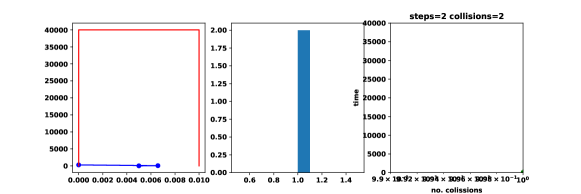
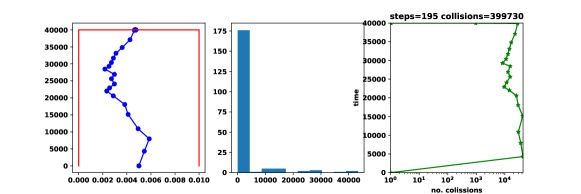
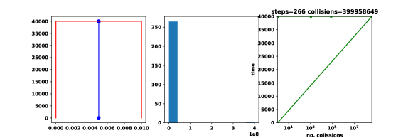
Figure 2: Examples of trajectories for the 1D $S_{2}$ test case with $L=0.01$, $T_{f}=40^{\prime}000$fs, $v=3.0\cdot 10^{-5}fs/cm$, $\sigma\in\{10^{-2}$, $10$, $10^{4}$, $10^{6}\}$ ($cm^{-1}$). Each row is a different value of $\sigma$. First column plots the particle evolution with $y$ axis being the time and $x$ axis the location in the $[0,L]$ segment. Second column displays the histogram of the $n_{c}$ values (cf algorithm A1.) The third column gives information on the total steps taken and total number of collisions treated.

For $\sigma=10^{-2}$ (first row of figures 2 and 3) the particle has very few collisions (here $2$) and exists the spatial domain well in advance of the final time $T_{f}$. The aggregation mechanism is never activated. The escape distributions concentrate on the borders $x=0$ and $x=L$; the middle column depicts the escape law conditional to having escaped because final time is reached; here this column has no mass at all.

For $\sigma=10^{1}$ (second row of figures 2 and 3) the computation can be accelerated by aggregating several collisions, up to $\simeq 40^{\prime}000$ for an average of $399730/195=2049$ collisions per step. The particular trajectory depicted here exists because final time is reached but $\simeq 14\%$ of trajectories exit because the spatial border is touched first.

For $\sigma=10^{4}$ and $\sigma=10^{6}$ (last two rows of figures 2 and 3) the particle undergoes an important number of collisions. The proposed procedure turns out to be very useful with a number of collisions per aggregated step being $399958649/266=1503603.94$ and $30000000317/371=80862534.55$ respectively. The procedure reaches thus acceleration factors of up to $10^{8}$ and the numerical resolution is very expensive without it. All particles exit because the time is up, none exists through the spatial borders: the particle behavior is that of a random walk around the initial point.

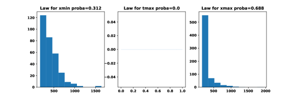
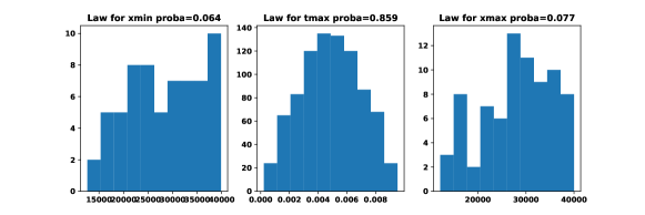
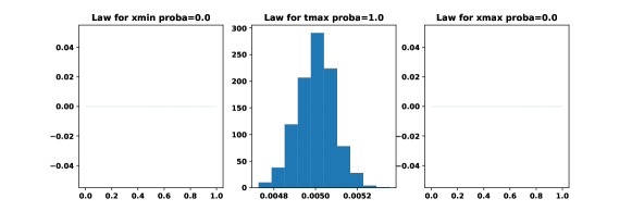
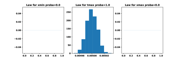
Figure 3:

3.2 One dimension, $N$ directions

We take now $N>2$ directions, i.e., the $S_{N}$ model. Such a model can for instance be used as a discretization of the situation when $\mathcal{D}$ is the whole unit sphere. We will not test the same things as before but instead investigate the two possible sources of error: the fact that $N$ is not $\infty$ and the fact that we used the normal approximation. Moreover we will take the most difficult test case which is the situation of a long time and a moderate value of $\sigma$, neither in the ballistic (small $\sigma$) nor in the diffusion (large $\sigma$) regime: $T=20^{\prime}000$fs, $\sigma=1$. The initial point is in the middle of the spatial interval ($x_{0}=L/2$).

We consider several test cases : parameters $N=10$ can be or $N=100$; the $n_{\mathcal{N}}$ parameter (that decides when the normal approximation is to be used) can be $n_{\mathcal{N}}=50$, $n_{\mathcal{N}}=300$ or $n_{\mathcal{N}}=1000$. In each case we compute $10^{\prime}000$ escape points $t,x,a$. The nominal values are : $n_{\mathcal{N}}=300$ cf. table 2 and $N=100$. The results for these nominal parameters are given in figures 4 and 5. It is seen in figure 4 that in this case all escape sides are populated, i.e., the particle can escape either through $x=0$ or $t=T$ or $x=L$. As expected the situation is symmetric and this is confirmed by the fact that the probability to exit though $x=0$ is the same as that for $x=L$ (up to precision $10^{-2}$). The figure 5 presents an example of trajectory. It is seen that the aggregation procedure has been effective because it reduced the total number of steps from $13692$ (the total number of collisions) to only $4122$. As expected, when the trajectory (the leftmost plot) approaches the boundary the collisions are treated one by one and when the trajectory is close to the middle of the interval almost $600$ collisions are aggregated together.

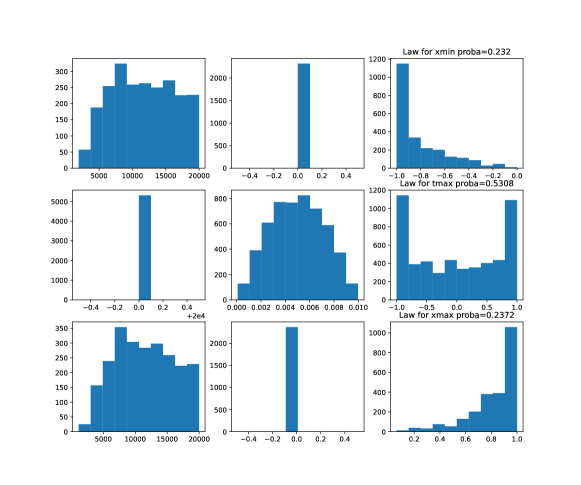
Figure 4: Results for the setting in section 3.2 for $n_{\mathcal{N}}=300$, $N=100$. The histograms of the escape distributions $t,x,a$ are plotted as follows: first column are the time values $t$, second column the positions $x$ and third the directions $a$. Each row is a conditional distribution : the first row are escape points with $x=0$, second row with $t=T$ and third with $x=L$.

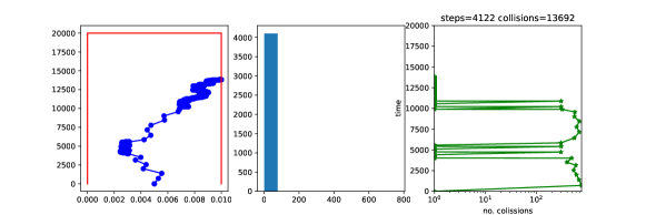
Figure 5: One example trajectory corresponding to results in figure 4, i.e. $n_{\mathcal{N}}=300$, $N=100$. Left plot: the trajectory of the particle, $y$ axis is the time. Middle plot: the distribution of the number of collisions that have been aggregated. Right plot: the number of collisions with time in the $y$ axis. Many are equal to $1$ but some go as high as $600-800$.

We make now variations around the nominal parameters. The results for $n_{\mathcal{N}}=1000$ and $N=100$ are given in figures 6 and 7. Here $n_{\mathcal{N}}$ is large enough so that all collisions are treated alone, no aggregation is used so the result is the one that we could have obtained without any aggregation procedure, cf. figure 7 middle where the histogram is a Dirac mass in $1$. On the other hand figure 6 shows that the escape distributions are very similar to that in figure 4 which shows that the aggregation procedure obtains comparable quality at lower costs. We have also tested $n_{\mathcal{N}}=50$ and $N=100$ and the results (not shown here) are the same as in 4 showing that our estimate $n_{\mathcal{N}}=300$ is actually a conservative one.

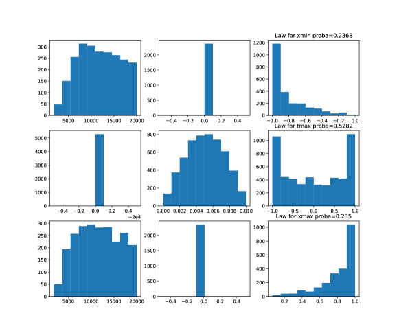
Figure 6: Results for the setting in section 3.2 for $n_{\mathcal{N}}=1000$, $N=100$.

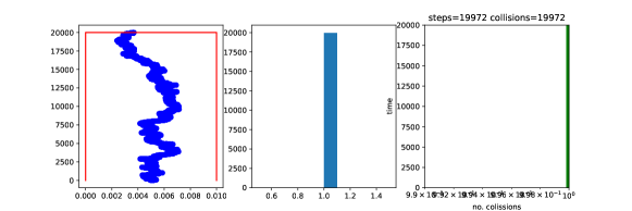
Figure 7: One example trajectory corresponding to results in figure 6, i.e., $n_{\mathcal{N}}=1000$, $N=100$. Signification of the plots is as in figure 5.

As a final test we will lower the parameter $N$ to inquire whether the escape distributions are sensitive to the discretization of the number of directions in $\mathcal{D}$. We take $N=10$, $n_{\mathcal{N}}=300$, results are in figures 8 and 9. Of course, the distribution in the third column of figures 8 is very discrete (only $10$ directions are possible and some of them coincide). But the reassuring result is that the other two columns look very much like that in figure 4 which shows that the discrete nature of $\mathcal{D}$ does not seem to play an important role in the shape of the escape distributions.

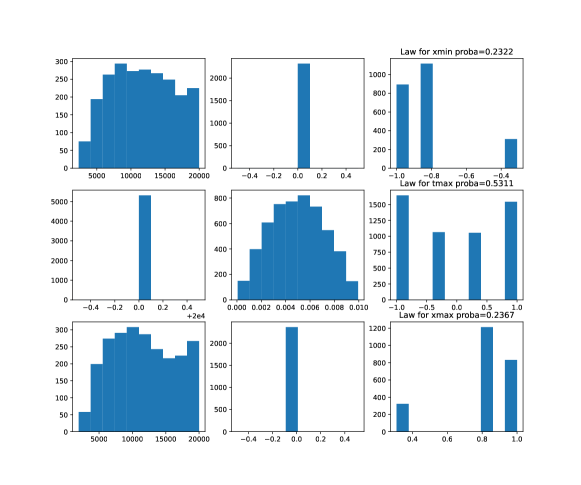
Figure 8: Results for the setting in section 3.2 for $n_{\mathcal{N}}=300$, $N=10$.

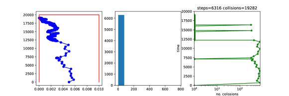
Figure 9: One example trajectory corresponding to results in figure 8, i.e., $n_{\mathcal{N}}=300$, $N=10$. Signification of the plots is as in figure 5.

4 Conclusions

We presented a method that accelerates the sampling of the escape times, position and directions for particles undergoing collisions separated by exponentially long times. The procedure works by aggregating several collisions into a single step. The advantage of the method is that it does not uses any model or random walk approximation and therefore can treat in the same way a large range of collision parameters where the random walk assumption could be unreliable. The procedure works by estimating conservatively the number of collisions that can safely be made before escaping the time-space domain; once this number estimated, the resulting position after those collisions is sampled exactly. The empirical results show that the numerical cost is substantially diminished while retaining excellent quality for the escape distribution.

References

- [1] Maria I. Cabrera, Orlando M. Alfano, and Alberto E. Cassano. Absorption and scattering coefficients of titanium dioxide particulate suspensions in water. The Journal of Physical Chemistry, 100(51):20043–20050, 1996.
- [2] Genyuan Li, Carey Rosenthal, and Herschel Rabitz. High dimensional model representations. The Journal of Physical Chemistry A, 105(33):7765–7777, 2001.
- [3] Jeffrey Shorter, Percila Ip, and Herschel Rabitz. Radiation transport simulation by means of a fully equivalent operational model. Geophysical Research Letters, 27(21):3485–3488, 2000.
- [4] J.A. Fleck and J.D. Cummings. An implicit Monte Carlo scheme for calculating time and frequency dependent nonlinear radiation transport. Journal of Computational Physics, 8(3):313 – 342, 1971.
- [5] E. D. Brooks III. Symbolic Implicit Monte Carlo. Journal of Computational Physics, 83(2):433–446, 1989.
- [6] B Lapeyre, É Pardoux, and R Sentis. Introduction to Monte-Carlo Methods for Transport and Diffusion Equations. Oxford University Press, July 2003.
- [7] E. W. Larsen. Diffusion theory as an asymptotic limit of transport theory for nearly critical systems with small mean free paths. Annals of Nuclear Energy, 7(4-5):249–255, 1980.
- [8] J.A. Fleck and E.H. Canfield. A random walk procedure for improving the computational efficiency of the implicit Monte Carlo method for nonlinear radiation transport. Journal of Computational Physics, 54(3):508–523, 1984.
- [9] J. Giorla and R. Sentis. A random walk method for solving radiative transfer equations. Journal of Computational Physics, 70(1):145–165, 1987.
- [10] Michael F Modest and Sandip Mazumder. Radiative heat transfer. Academic press, 2021.