Neural Networks Hear You Loud And Clear: Hearing Loss Compensation Using Deep Neural Networks

Abstract

This article investigates the use of deep neural networks (DNNs) for hearing-loss compensation. Hearing loss is a prevalent issue affecting millions of people worldwide, and conventional hearing aids have limitations in providing satisfactory compensation. DNNs have shown remarkable performance in various auditory tasks, including speech recognition, speaker identification, and music classification. In this study, we propose a DNN-based approach for hearing-loss compensation, which is trained on the outputs of hearing-impaired and normal-hearing DNN-based auditory models in response to speech signals. First, we introduce a framework for emulating auditory models using DNNs, focusing on an auditory-nerve model in the auditory pathway. We propose a linearization of the DNN-based approach, which we use to analyze the DNN-based hearing-loss compensation. Additionally we develop a simple approach to choose the acoustic center frequencies of the auditory model used for the compensation strategy. Finally, we evaluate the DNN-based hearing-loss compensation strategies using listening tests with hearing impaired listeners. The results demonstrate that the proposed approach results in feasible hearing-loss compensation strategies. Our proposed approach was shown to provide an increase in speech intelligibility and was found to outperform a conventional approach in terms of perceived speech quality.

I Introduction

Hearing loss is a debilitating disease, affecting almost 500 million people worldwide [1]. Hearing loss is usually managed by prescription of hearing aid (HA) devices that amplifies acoustic sounds to make them audible by the afflicted patients. These devices usually consist of a system that can provide noise reduction (NR), to reduce the effect of background noise and competing speakers, followed by compressive amplification, that attempts to restore the loudness perception within the limited dynamic range of a HA user with impaired hearing. In recent years, auditory models have been developed that simulate the complex, non-linear behaviour of neural representations of the auditory pathway when excited by acoustic stimuli. Although these models have been able to represent increasingly complex auditory phenomena, it is not clear how these representations can be translated into practical signal-processing strategies, as the neural-representations are highly non-linear and extremely computationally expensive to generate. Recently, a methodology for emulating auditory models with high degrees of hearing loss and high dynamic range has been developed, allowing deep neural networks to emulate the auditory models end-to-end, decreasing inference time by several orders of magnitudes [2]. This methodology allows the use of the auditory models for the purpose described in this work, namely developing hearing-loss compensation (HLC) and NR-strategies, using the outputs of the auditory models as biologically inspired optimization objectives. Ideally, this optimization restores the output of the hearing-impaired representation to that of normal hearing, hypothesising that this strategy will enhance the hearing abilities of hearing-impaired individuals, as compared to conventional HLC or NR strategies. Such an approach, if successful, would allow for development of perceptually relevant signal-processing strategies, but also the personalization of HLC and NR to the individual dysfunction of the auditory pathway. Although similar approaches to hearing-loss compensation have been suggested several times before [3, 4, 5, 6, 7], to our knowledge no evidence in terms of human listening tests have been presented that suggest this approach is successful. In this work, we develop deep neural network based HLC and NR strategies using an auditory-nerve model. First the auditory models and compensation strategies are analyzed using a linearized closed-form model, which can be used to guide hyperparameter choices of the DNN-based HLC and NR strategies. Next, the developed HLC and NR strategies are trained using these choices, evaluated and compared to conventional strategies using subjective tests in terms of intelligibility and sound-quality assessment on a group of hearing-impaired individuals.

The article is structured as follows: We shortly introduce conventional hearing loss compensation schemes in Sec. II. In Sec. III we introduce a framework to emulate an auditory-nerve model using DNNs in . Thirdly, a linearized model of an auditory-model based hearing-loss compensation is introduced in Sec. IV, which allows us to analyze the linear effects of the DNN-based compensation strategy and choose hyperparameters for finding the final DNN-based HLC strategy. In Sec. V we introduce the DNN architectures used for HLC and how we train these networks. The listening experiments are presented in Sec.VI, and evaluated in VII where we compare conventional HLC and NR to our proposed auditory-model based HLCs, using listening experiments on hearing impaired subjects. In Sec. VIII we discuss the results and their implications, possible limitations and perspectives for future work. Finally, in Sec. IX we provide a short overview of our findings, concluding our work.

II Conventional hearing-loss compensation strategies

Conventional hearing-loss compensation strategies can usually be grouped into either loudness-normalization (LN) rationales or loudness-equalization (LE) rationales. The goal of a LN rationale is to restore the perceived loudness perception in each frequency band. A ”soft”, ”medium” or ”loud” narrow band sound for a normal hearing individual should be perceived equivalently as a ”soft”, ”medium” or ”loud” narrow band sound for the HA user wearing a hearing aid. Secondarily, the relative loudness between frequency bands should not change. The goal of a LE rationale is on the other hand that the HA user should perceive all frequency bands as equally loud, which is argued to increase speech intelligibility [8]. One such LE rationale is the NAL-Revised (NAL-R) [9], that provides a linear time-invariant gain, parameterized by the pure-tone audiogram of the HA user. However, because shifts in hearing thresholds often are not accompanied by similar shifts in thresholds of discomfort at loud levels, hearing impairment results in a reduced dynamic range. To address the reduced dynamic range of the HA user, modern hearing aids employs a wide dynamic range compression (WDRC) scheme[10]. The fitting rationales for WDRC-based hearing-loss compensation strategies provides different frequency/gain curves at different sound pressure levels (SPLs), in particular higher gains at lower SPLs. However, while fitting rationales provide general guidelines, the specific implementation of WDRC systems can differ between manufacturers and hearing aids, resulting in essentially differing - and proprietary - hearing-loss compensation strategies, using the same fitting rationale [11]. In particular, multi-band compression schemes are frequently employed in hearing aids due to their ability to provide precise control over compression in distinct frequency bands. This approach helps prevent the negative impact of transients on speech cues located at lower frequencies, while also accommodating the dynamic ranges present at different frequency regions, which depends on the particular hearing loss [12][13].

III Auditory-model emulation

In this section we will explain the particular auditory model used for this work, the Zilany model [14], and how we emulated it using deep neural networks. Additionally, we introduce the Verhulst auditory model[15], which we use for our linear-model analysis in Sec. IV . First, we define a generic notation, that will be used when describing auditory models in this work: Consider an acoustic signal space $X\subset\mathbb{R}^{T}$, and an inner representation space $I\subset\mathbb{R}^{K\times T}$, where $K$ denotes the number of frequency-channels and $T$ is the number of time-samples. The auditory model is defined as $f^{\theta}:X\rightarrow I$, where $\theta$ is a vector containing the free parameters of the auditory model. Additionally, when $\theta=\textrm{NH}$ it denotes the particular parameters determining a normal hearing representation and when $\theta=\textrm{HI}$ it denotes the parameters determining a hearing-impaired representation. We denote the $k$-th channel as $f_{k}$.

III-A The Zilany model

The Zilany model is an auditory model that simulates the auditory-nerve response to an acoustic signal [14]. The model comprises multiple stages of the auditory pathway, including a middle-ear stage, a combined cochlea stage that mimics the behavior of outer hair cells (OHCs) and inner hair cells (IHCs), and an IHC-to-auditory nerve synapse (IHC-AN) stage, which we use to model the expected firing rate of the auditory nerve. An implementation of the model can be found at [16], and an overview of the model can be seen in Figure 1.

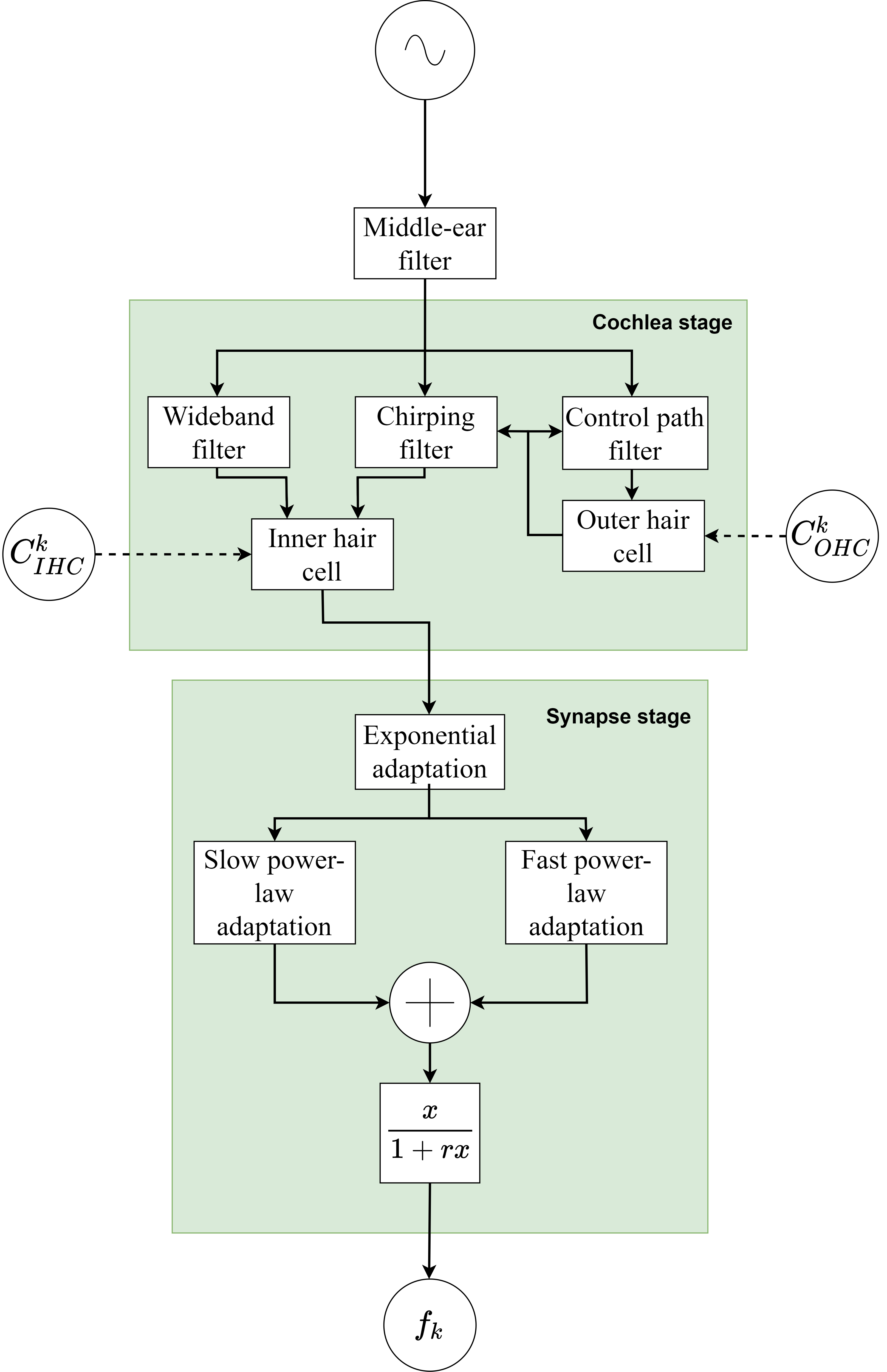
Figure 1: Overview of the Zilany model

The Zilany model can be partitioned into the following stages:

III-A1 Middle-ear stage

The middle ear is a linear circuit-model, implemented as a set of cascaded filters, that simulates the forward transmission from the ear canal to the oval window, followed by the cochlea stage.

III-A2 Cochlea stage

This stage consists of two branches 1) A chirping filter, where the gain and bandwidth of the filters are controlled by the input SPL through the control signal path, simulating the level-dependent properties of the cochlea, and 2) a linear, static filter that dominates at high levels. The outputs of both filters are fed through their individual transduction functions, such that they combine to generate the IHC potential.

III-A3 Synapse stage

The IHC-AN synapse stage is a power-law adaptation (PLA) model, that consists of an exponential adaptive stage that drives two parallel power-law adaption paths, a slow and a fast path [17]. In the original model, a fractional noise is used to model the time-varying distribution of the spontaneous rate. However, in this work we are only interested in the deterministic response to stimuli, particularly speech, and thus this noise process was omitted. Finally, the output of the synapse, $x$ is processed by a rational function, $x(1+rx)^{-1}$, that converts the synapse output to an expected value of the time-varying rate function of the auditory nerve. The synapse stage is parameterized by the spontaneous firing rate of the auditory nerve-fiber. For this work we simulate auditory nerve fibers with low-, medium and high spontaneous rates, corresponding to different synaptic characteristics. For each of the fibers we compute a reference response with zero input, resulting in the spontaneous activity that is not driven by the fractional Gaussian noise. The reference response is subtracted from the response to any stimulus, resulting in a stimulus response that is zero when the input is zero.

In order to model hearing losses in the Zilany model, a function, ”fitaudiogram2”, is provided with the auditory model code. This function takes a pure-tone audiogram (PTA) as input and produces the parameters for OHCs and IHCs for each characteristic frequency (CF). A PTA measures hearing loss relative to normal hearing and is defined for 10 frequency bands. We distribute 2/3 of the hearing loss to OHCs and 1/3 to IHCs for all audiograms, which is the default setting in the ”fitaudiogram2” function. The parameters are denoted as $C_{OHC}(k)\in[0,1]$ and $C_{IHC}(k)\in[0,1]$, representing two parameters for each CF, with 0 indicating complete dysfunction and 1 representing normal hearing. Additonally, we smooth $C_{OHC}(k)$ and $C_{IHC}(k)$ across CFs using a 3-point moving average.

III-B The Verhulst model

The Verhulst model is an alternative auditory model of the auditory pathway, that consists of a transmission-line model of the basilar membrane, an IHC stage, an auditory-nerve stage, and a midbrain stage [15]. Hearing loss can be emulated by parameterizing the non-linearities of the outer hair cells in the model, such that the amplitude response, at a given CF, to a single tone is reduced by the specified loss. The model only captures hearing loss attributed to OHCs, which is maximally 35 dB at every CF[18], and synaptopathy (permanent loss of synapses in the auditory nerve) , which can be modelled by reducing the number of nerve fibers in the auditory-nerve stage. Since there is no established way to parameterize larger, clinically relevant hearing losses for the Verhulst auditory model, we opted to used the Zilany model to generate the final HLC and NR strategies, cf. Sec. V, but we use the Verhulst auditory model for comparison with previously devloped DNN-based HLC systems [7].

III-C Auditory Model Emulators

In order to decrease the computational time required for the auditory model to process an input signal and generate the inner representation, i.e. the auditory-nerve firing rate (the forward pass) and the computation of the partial derivative of the model with respect to the input signal (the backward pass), we simulate the auditory model using a feed-forward convolutional neural network, which we call an auditory-model emulator (AME).

An AME can be trained for each individual subject. All AMEs are trained using the same procedure, hyperparameters and speech dataset, the LibriTTS dataset[19], using 4000 utterances for the training set, and 500 utterances for the validation set. In general, training such an AME is not straightforward, for the following reasons:

1. Initial pilot-experiments found that the auditory models were sensitive to choice of hyperparameters. Thus, finding suitable architectures and hyperparameters is non-trivial.

2. The DNN must be able to emulate the auditory model across all auditory-model channels and different types of inputs.

3. Conventional training methods of deep neural networks induces a bias towards producing a low-frequency representation of the target function, meaning that certain output channels of the auditory-model emulator will converge faster to the ground-truth auditory model, even if all the frequency components are energy-normalized[20].

Thus, these three issues had to be addressed during training and model tuning. We addressed these issues individually in the following way:

III-C1 Finding a suitable architecture

Finding a suitable architecture for an AME is largely an empirical process. There are some constraints, such as having a large enough receptive field to properly model the time constants of the original auditory model. Furthermore, feed-forward convolutional models are good candidates, since they impose a translational equivariance prior on the DNN, also reflected in the auditory model. An auto-encoder structure allowed for efficient representations of the long time constants of the auditory model, which motivated us to choose the Wave-U-Net, a convolutional auto-encoder. The hyperparameters are shown in Table I. We found that different activation functions could lead to vastly differing performance. Based on experimental work we choose the hyperbolic tangent (Tanh) activation in the encoder (all the downsampling blocks) and the PReLU activation [21] in the decoder (all the upsampling blocks and the embedding block). With the hyperparameters shown in Table I, we achieved a receptive field large enough to model the longer time constants in the auditory model.

III-C2 Ensuring equal performance across channels and inputs

To achieve good performance across auditory model channels and inputs of different SPLs, we train the network using the Frequency and level-dependent mean-absolute error (FMAE) [2], which normalizes the error across input levels and auditory model channels:

$$\leavevmode\resizebox{216.81pt}{}{$\mathrm{FMAE}(f(\textbf{x}_{l}),\bar{f}(\textbf{x}_{l});\beta_{k},\alpha_{k,l})=\dfrac{1}{TK}\sum\limits_{k=1}^{K}||\beta_{k}f_{k}(\textbf{x}_{l})-\bar{f}_{k}(\textbf{x}_{l})||_{1}\alpha_{k,l}$}\,,$$ (1)

where $\alpha_{l,j}$ and $\beta_{j}$ are parameters related to the distribution of energy in the inner representation of the auditory model. Furthermore, we also applied the following augmentations to the dataset used to train the AME: Addition of babble noise and speech-shaped Gaussian noise at a large range of SNRs, band-pass filtering with either band-pass or high-pass filtering of the noisy speech, using random widths and center frequencies, before processing the noisy speech by the auditory model. Additionally, the auditory models were trained with inputs normalized to sound pressure levels (SPLs) between 55 and 95 dB SPL.

III-C3 Adressing the frequency bias of the AME

To address the issue of frequency bias in the training of the AME, we started with small batch sizes, for faster convergence and increased the batch size if the validation error did not increase for 5 epochs. The batch size was increased until the capacity of the GPU memory was reached (24 GB). The small batch size enables training of the the model within a reasonable time-frame, while increasing the batch-size as the model is closer to convergence, exploits the fact that larger batch sizes tend to decrease the frequency bias, which was verified during pilot experiments.

TABLE I: Network parameters of the AME. N denotes the number of Upsampling/Downsampling blocks.

N	8
Kernel size	21
Depth	128
Encoder activation	Tanh
Decoder activation	PReLU
Bias	False

IV Auditory-model-based hearing-loss compensation

In this section we present the proposed hearing-loss compensation strategies, using auditory models. In particular, we first derive linear compensation strategies to predict some of the behaviour of the generally non-linear deep-learning-based compensation strategies and to guide hyperparameter choices for the DNN-based hearing-loss compensation strategies.

Hearing-loss compensation strategies can be trained, by finding a function that transforms an acoustic signal to minimize a difference between the output of a normal-hearing auditory model and a hearing-impaired auditory model, cf. Fig. 2.

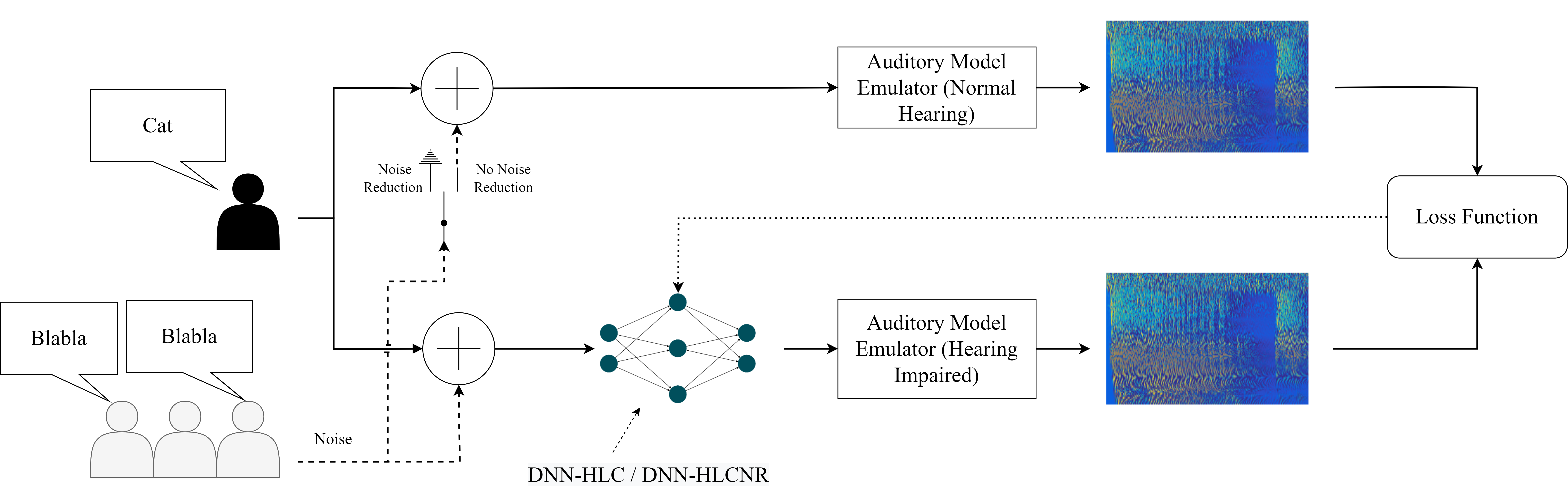
Figure 2: An overview of how a deep-neural-network based hearing-loss compensation (DNN-HLC / DNN-HLCNR) is trained. In each step, speech material passes through a normal hearing auditory model emulator (NH-AME). Noise is added to the upper branch when training the DNN-HLC, and there is no noise added when training the DNN-HLCNR. The noisy speech material is fed through the DNN-HLC(NR), and the output of the DNN-HLC(NR) is fed through a hearing impaired auditory model emulator (HI-AME). The output of the NH-AME and HI-AME is compared through a loss function, which is minimized by iteratively updating the weights of the DNN-HLC(NR), through the derivative of the loss function.

A transformation that minimizes this difference is called an optimal compensation strategy. To find such an optimal compensation strategy, one can use DNNs, as they are universal function approximators [22], and in theory a DNN can model such an optimal compensation strategy efficiently - if it can be found. For the following, we use the notation explained in Sec. III. First, define a compensation strategy as a function $c:X\rightarrow X$. To find an optimal compensation strategy, we want to find the function $c(\cdot)$ that minimizes:

$$L(f^{\textrm{NH}}(\textbf{x}),f^{\textrm{HI}}(c(\textbf{x})))$$ (2)

where $L:I\times I\rightarrow\mathbb{R}$ is some measure of dissimilarity - a loss function in optimization terminology - and x is an acoustic signal, $\textbf{x}\in X$. In this work we focus on auditory models that simulates the physiological response of the peripheral auditory system, e.g., the response to an acoustic signal as basilar membrane vibrations or auditory-nerve firing rates.

IV-A Optimal linear compensation strategies

Before dealing with the problem of optimizing for non-linear auditory models and DNN-based HLCs, it is useful to consider simplified, linear auditory models that admits optimal and linear solutions. In order to find optimal, linear compensation strategies we can consider the conventional squared Euclidean distance as a dissimilarity measure. The squared Euclidean distance is equivalent to the often used mean-squared error and admits simple, closed-form solutions for linear and time-invariant systems. For inner representations stored in matrices, the mean-squared error is equivalent to the squared Frobenius norm. Let N and D be linearizations of the normal and hearing-impaired auditory model respectively at some SPL relevant for speech (e.g. 65 dB SPL), i.e $\textbf{N},\textbf{B}\in\mathbb{R}^{K\times T}$. If we consider a linear and time-invariant implementation of an auditory model, and we define the auditory models as the linear convolution between each auditory frequency channel and a signal x, the inner representation is given by:

$$f_{lin}^{NH}(\textbf{x}) =\textbf{N}\mathbb{T}(\textbf{x})$$ (3)

$$f_{lin}^{HI}(c(\textbf{x})) =\textbf{D}\mathbb{T}(c(\textbf{x}))$$ (4)

$$c(\textbf{x}) =\textbf{c}*\textbf{x}=\mathbb{T}(\textbf{x})^{T}\textbf{c}\,,$$ (5)

where $\textbf{c}\in\mathbb{C}^{T}$ and $\mathbb{T}(\cdot)$ is the operator that transforms a vector into its Toeplitz matrix, i.e:

$$\mathbb{T}(\textbf{x})=\begin{bmatrix}x_{1}&x_{2}&\ldots&x_{T}\\ 0&x_{1}&\ldots&x_{T-1}\\ \vdots&\vdots&\ddots&\vdots\\ 0&\ldots&0&x_{1}\end{bmatrix}\,.$$ (6)

Then, we find a MSE-optimal, linear compensation strategy, c, as:

$$\textbf{c}=\displaystyle{\operatorname*{arg\,min}_{\textbf{c}\in\mathbb{R}^{T}}}||\textbf{N}\mathbb{T}(\textbf{x})-\textbf{D}\mathbb{T}(\mathbb{T}(\textbf{x})^{T}\textbf{c})||_{F}^{2}$$ (7)

Let $\textbf{W}\in\mathbb{C}^{T\times T}$ denote the discrete Fourier transform matrix, such that the discrete Fourier transform along each row of N is given by $\textbf{N}\textbf{W}^{T}$, and the Fourier transform of a vector, x, is given by Wx. Define $\tilde{\textbf{N}}=\textbf{N}\textbf{W}^{T}$, $\tilde{\textbf{D}}=\textbf{D}\textbf{W}^{T}$, $\tilde{\textbf{x}}=\textbf{W}\textbf{x}$ and $\tilde{\textbf{c}}=\textbf{W}\textbf{c}$, Using Parseval’s theorem, one can show that Eq. 7 is equivalent to:

$$\tilde{\textbf{c}}=\displaystyle{\operatorname*{arg\,min}_{\tilde{\textbf{c}}\in\mathbb{C}^{T}}}||\tilde{\textbf{N}}\textrm{diag}(\tilde{\textbf{x}})-\tilde{\textbf{D}}\textrm{diag}(\tilde{\textbf{x}})\textrm{diag}(\tilde{\textbf{c}})||_{F}^{2}\,.$$ (8)

Solving for c leads to:

$$\tilde{\textbf{c}}=(\tilde{\textbf{D}}^{H}\tilde{\textbf{D}}\odot\textbf{I})^{-1}(\tilde{\textbf{D}}^{H}\tilde{\textbf{N}}\odot\textbf{I})\textbf{1}$$ (9)

or equivalently for each frequency bin, $i$, as:

$$\tilde{\textbf{c}}_{i}=\dfrac{\tilde{\textbf{D}}_{i,:}^{H}\tilde{\textbf{N}}_{:,i}}{\tilde{\textbf{D}}_{i,:}^{H}\tilde{\textbf{D}}_{:,i}}\,,$$ (10)

with $(\cdot)^{H}$ denoting the Hermitian transpose, $\odot$ the Hadamard product, I the identity matrix , 1 the vector containig all ones, $\textbf{N}_{i,:}$ the column-vector at the i-th row, and $\textbf{N}_{:,i}$ the row vector at the i-th column. Eq. 10 shows that an optimal MSE time-domain solution is equivalent to finding, for each frequency bin, a complex scalar gain that is applied to every channel of the auditory model. Eq. 8 implies that hearing loss can only be completely restored if $\tilde{\textbf{N}}=\tilde{\textbf{D}}\textrm{diag}(\tilde{\textbf{c}})$, i.e. the relation between the normal and hearing-loss model is such that, for all frequency bins, each auditory filter is multiplied by the same factor. This could be achieved in two ways: 1) If all channels are orthogonal or 2) if D is generated from N by the same linear transformation applied to all CFs, i.e. each row of N, both 1) and 2) resulting in unrealistic implementations of auditory models or hearing losses. This result implies that, in general, realistic hearing losses can not be completely restored in a squared-error sense.

IV-B A comparison of Linear HLCs and DNN-based HLCs

When training a deep-learning based compensation strategy we observed - under some circumstances - an undesirable ripple-like structure in the long-term linear frequency-gain (g) of the compensation strategy:

$$\textbf{g}=E[|\textbf{W}c(\textbf{x})|]\oslash E[|\textbf{W}\textbf{x}|]\,,$$ (11)

where $\oslash$ denotes component-wise division and $E[\cdot]$ is the expected value (for our experiments, we used Welch’s method [23] as an estimator). We hypothesize that the ripple structure is a linear effect caused by some frequencies not being represented adequately in common loss functions, and therefore can be modelled by Eq. 8. In that case, the MSE will be greatest around the peaks, as compared to in-between the peaks, and thus one should expect a comb-like ripple structure of g if one uses too few CF’s. We hypothesize that the locations of the peaks of this ripple-structure will be determined exactly by the locations of the CFs, and the shape of this ripple-structure will be determined by the specific auditory model, the hearing loss and the loss function. We verify our hypothesis by testing two different scenarios: 1) Training a compensation strategy based on the Zilany auditory model, using a DNN (see Sec. V for DNN architecture and training) and 2) comparing with a previously trained DNN trained on a different auditory model - the Verhulst auditory model - using a different loss function.

IV-B1 Comparison of the linear model with a DNN-based HLC using tthe Zilany auditory model

In Fig. 3 we show a comparison of the linear HLC based on Eq. 8 with a DNN-based HLC strategy, using a flat hearing loss of 40 dB. We see that the gain of the linear model matches the gain of the DNN-based HLC fairly well, particularly when it comes to the size and peaks of the ripple-like structure.

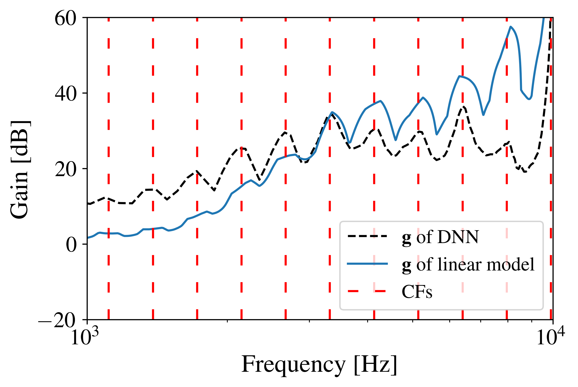
Figure 3: Long-term average gain of a DNN-based hearing loss compensation strategy, optimized at the auditory nerve level of the Zilany model and a linear, optimal gain, based on a 40 dB flat hearing loss.

IV-B2 Comparison of the linear model with a DNN-based HLC using the Verhulst auditory model

In Fig. 4 we show a comparison of the linear model based on Eq. 8 with a DNN-based hearing-loss compensation strategy (DNN-HA) from [24]. DNN-HA is optimized on 21 CFs using a composite loss function, based on absolute differences of different features at the auditory nerve-level and a 35 dB Flat hearing loss. Even though the optimization objectives are very different, we find that the optimal, linear gain can predict the long-term ripple structure of the signals processed by the DNN-HA.

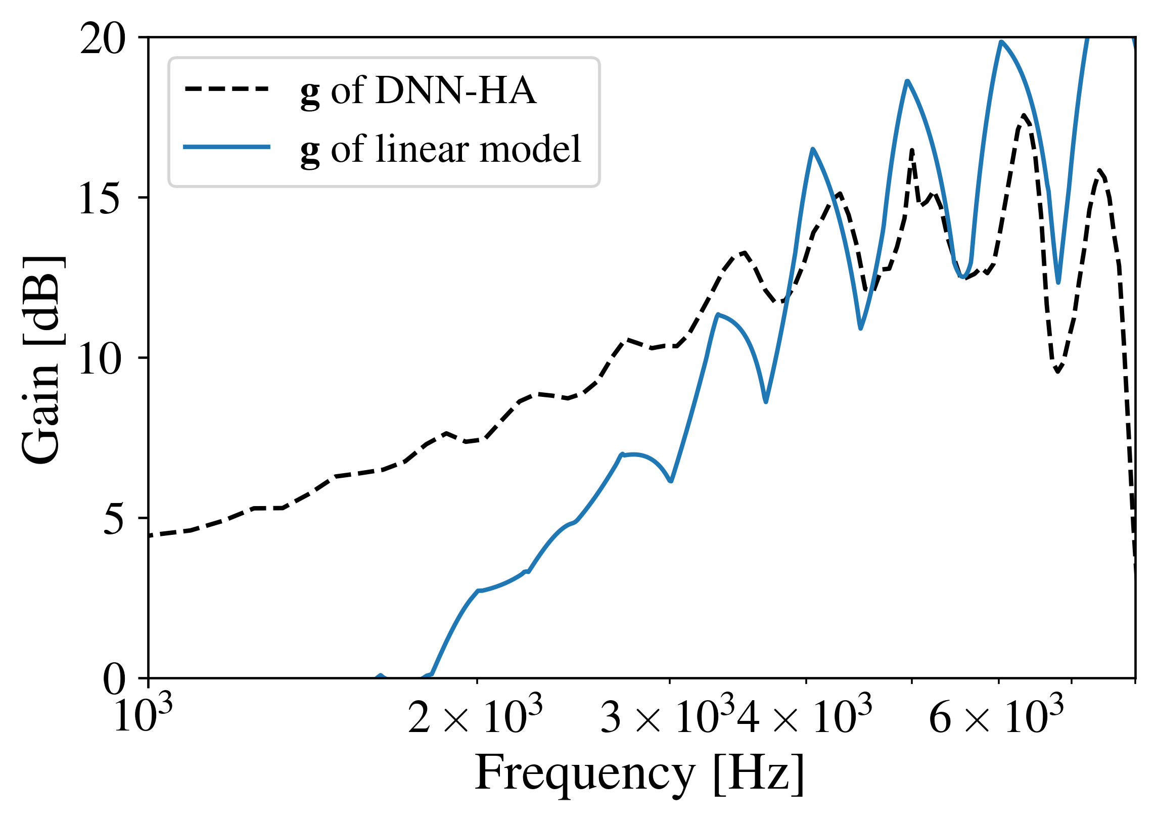
Figure 4: Gain of the DNN-HA, optimized at the auditory nerve level of the Verhulst model using a composite loss function and a linear, optimal gain, based on a 35 dB flat hearing loss.

IV-C Choosing appropriate CFs

An optimal spacing of the CFs will depend on the particular auditory model, and the amount of ripple one can allow. Thus, to construct a set of center frequencies we propose a simple algorithm that, recursively builds a list of center frequencies, by making sure that the amplitude response at the next CF only decays a certain amount from the peak as determined by $\Delta$, see Algorithm 1.

input : $\text{CF}_{min}$, $\text{CF}_{max}$, $\Delta$

output : A set of center frequencies, spanning $\text{CF}_{min}$ to $\text{CF}_{max}$

$v\leftarrow\text{CF}_{min}$;

CFs $\leftarrow$ list;

while $v<\text{CF}_{max}$ do

       $\textbf{z}\leftarrow\textrm{frequencyResponse}(f_{k}^{NH};\textrm{CF}(k)=v)$;

       find smallest $\text{freq}({i})>v$, s.t. $\dfrac{\textrm{abs}(\textbf{z})_{i}}{\textrm{max}(\text{abs}(\textbf{z}))}<\Delta$ ; AppendToCFs(v);

       $v\leftarrow\text{freq}(i)+v-\text{freq}(\text{argmax}(z))$;

      

end while

Algorithm 1 Algorithm to select CFs. Here freq(i) denotes the frequency of the i-th index, CF(k) denotes the CF of the k-th channel.

An example comparison of the conventional log-spacing and our proposed spacing can be seen in Fig. 5. To better see the effect of our proposed spacing strategy as a function of the number of channels, K, we propose using a normalized error, defined as the gain-to-ripple-ratio (GNR), i.e:

$$\textrm{GNR}(\textbf{g}^{ref},\textbf{g})\stackrel{{\scriptstyle\text{def}}}{{=}}10\log_{10}\left(\dfrac{||\textbf{g}^{ref}||_{2}^{2}}{||\textbf{g}^{ref}-\textbf{g}||_{2}^{2}}\right)$$ (12)

where $\textbf{g}^{ref}$ is the gain of a reference compensation strategy, which can be computed using a large amount of CFs, and g is the gain of some proposed compensation strategy. In Fig. 6, we compare the GNR of a log spacing and our proposed spacing, using the output of the chirping filter of the Zilany model, see Fig. 1, which is the primary contributor to the frequency tuning of the model, using a N3 hearing loss [25]. We find that our proposed spacing shows less ripple than the log-spaced CFs. Furthermore, Fig. 6 also shows that increasing the number of CFs decreases the ripple of the optimal-compensation gain curve, as expected.

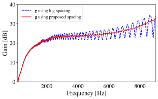
Figure 5: Comparison of optimal-compensation insertion gains for the output of the chirping filter of the Zilany auditory model, using K=96 CFs and a moderate hearing loss, N3 [26]. The proposed spacing can be generated by using Algorithm 1.

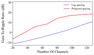
Figure 6: Gain-to-ripple ratio calculated using the output of the chirping filter in the Zilany auditory model, with the hearing impaired representation parameterized by a N3 audiogram [26]. The CFs are generated with $\textrm{CF}_{min}=125\textrm{ Hz}$ and $\textrm{CF}_{max}=9900\textrm{ Hz}$. The reference, $c_{ref}$, is generated using K = 385 CFs, corresponding to $\Delta=0.95$ in Algorithm 1, which also shows how to generate the proposed spacing.

V Compensation networks

In this section, we will present the particular neural networks and the loss functions that were used for the DNN-based HLCs developed in this paper. Additionally, we present an extension to the DNN-HLC where noise is added to the lower branch, thus the resulting DNN-HLC also provides noise reduction. We call this network ”deep-neural-network-based joint hearing-loss compensation and noise reduction” (DNN-HLCNR).

V-A Architecture of the DNN-HLC

For the DNN-HLC we use the same neural network as was used for the AME, the Wave-U-Net [27], with parameters found in Table II. These parameters were found during pilot tests, both by observing convergence of loss functions, and by informal listening tests. Due to the structure of the experiments, it was also paramount that the neural networks could be trained fast and efficiently, which is why we opted for the Wave-U-Net, which has a relatively low memory footprint, allowing for better parallelization, thus speeding up the training process.

TABLE II: Network parameters of the DNN-HLC. N denotes the number of Upsampling/Downsampling blocks.

N	6
Kernel size	9
Depth	128
Encoder activation	Tanh
Decoder activation	PReLU
Bias	None

V-B Loss function for auditory-model based DNNs

The derivative of a given parameter $\phi$, e.g. a weight of a DNN, of a parametric compensation strategy, $c(\textbf{x};\phi)$ with respect to a loss function $L$ is given by:

$$\dfrac{\delta L(f^{NH}(\textbf{x}),f^{HI}(c(\textbf{x};\phi)))}{\delta\phi}=$$

$$\dfrac{\delta L(f^{NH}(\textbf{x}),f^{HI}(c(\textbf{x};\phi)))}{\delta f^{HI}(c(\textbf{x};\phi))}\dfrac{\delta f^{HI}(c(\textbf{x};\phi))}{\delta c(\textbf{x};\phi)}\dfrac{\delta c(\textbf{x};\phi)}{\delta\phi}$$ (13)

Note that the derivative can only be computed if the individual terms are tractable. In particular, calculating the second term of Eq. V-B, $\dfrac{\delta f^{HI}(c(\textbf{x};\phi))}{\delta c(\textbf{x};\phi)}$, requires the auditory-model to be differentiable. While the original auditory models might not be differentiable, the auditory model emulator is differentiable, because it is emulated by a differentiable DNN.

One such loss function is the the Mean-absolute error (MAE) - with the derivative set to zero at the origin - computed between the two inner representations:

However, such a loss function might be sensitive to minor phase differences between the two inner representations. Therefore, we modify the loss function by average pooling of the inner representation, i.e. segmenting the temporal representation into frames of a given length, and averaging each frame. Define:

$$y_{k,i}^{NH} =\frac{1}{f_{s}D}\sum_{m=1}^{f_{s}D}f_{k}^{NH}(\textbf{x})[(i-1)f_{s}D+m]$$ (15)

$$y_{k,i}^{HI} =\frac{1}{f_{s}D}\sum_{m=1}^{f_{s}D}f_{k}^{HI}(c(\textbf{x};\theta))[(i-1)f_{s}D+m]\,$$ (16)

where $D$ is the length of each frame in milliseconds, $f_{s}$ the sampling rate and the square brackets denote the given index of a vector. Then, we have.

$$\small L_{MAE,D}=\frac{1}{K}\sum_{k=1}^{K}\frac{f_{s}D}{T}\sum_{i=1}^{\dfrac{T}{f_{s}D}}\left|y_{k,i}^{NH}-y_{k,i}^{HI}\right|\,.$$ (17)

We compute the MAE at three time-scales, 1 ms, 10 ms and 100 ms. We denote these as $L_{MAE,1}$, $L_{MAE,10}$ and $L_{MAE,100}$ respectively. In order to avoid spurious low-frequency behaviour that is not properly captured by the auditory model, we include a term to penalize low-frequency energy:

$$L_{f}(\textbf{x},c(\textbf{x}))=\sum_{i}||(\textbf{W}\textbf{x})_{i}-\textbf{W}(c(\textbf{x};\theta))_{i}||_{1}\,,\,\,\mathrm{freq}(i)<50\textrm{Hz}\,,$$ (18)

where $\textrm{freq}(i)$ is the frequency of the i-th index of the discrete Fourier transform. We combine the loss functions:

$$L=L_{MAE,1}+L_{MAE,10}+L_{MAE,100}+\gamma L_{f}$$ (19)

where $\gamma$ is a small constant, found during pilot experiments.

V-C Architecture of the noise-reduction networks

Noise reduction is an important part of every HA, and NR algorithms based on DNNs are ubiqutous in the literature, therefore we extend our HLCs to include NR networks: A generic NR network that is trained using an ubiquitous loss function, and our proposed network, the joint DNN-based HLC and NR, DNN-HLCNR. For the two noise-reduction networks we use identical architectures, a variation of the Conv-TasNet [28] that is more memory efficient, SuDORMRF [29]. The neural network consists of an encoder that downsamples a noisy acoustic signal, followed by a separator that calculates a non-negative mask which is applied to the encoded representation of the acoustic signal, resulting in a denoised, encoded representation of the acoustic signal. Finally, the denoised representation is upsampled by the decoder, resulting in the denoised acoustic signal.

V-D Loss functions for noise reduction

Conventional deep neural networks for noise reduction (DNN-NR) can be trained using a diverse set of loss functions [30]. One such loss function, commonly used in the state-of-the-art DNN-NRs, is the scale-invariant signal-to-distortion ratio (SI-SDR) [31]:

$$\text{SI-SDR}(\textbf{s},\hat{\textbf{s}})=10\log_{10}\dfrac{||\dfrac{\hat{\textbf{s}}^{T}{\textbf{s}}}{||\textbf{s}||_{2}^{2}}||_{2}^{2}}{||\dfrac{\hat{\textbf{s}}^{T}\textbf{s}}{||\textbf{s}||_{2}^{2}}-\hat{\textbf{s}}||_{2}^{2}}$$ (20)

where s is the target signal of interest, and $\hat{\textbf{s}}$ is the estimated denoised signal, e.g. the output of a DNN-NR.

V-E Training

All the DNNs were trained using 8000 utterances for the training set and 2000 utterances for the validation. All utterances were sampled from LibriTTS [19], and were utterances that were not seen during training the AMEs, cf. Sec. III. All utterances were normalized to a sound pressure level (SPL) of 65 dB. Two different noise types were used: 16-speaker babble noise and stationary, Gaussian, speech-shaped noise. The SNRs were randomly selected from a wide range of SNRs that were relevant for the listening experiments (0, 3, 6, 9, 12, 100), thus the networks were exposed to both clean and noisy speech, which could be important for the DNN-HLC and the DNN-HLCNR. Note, that even though the SNR could be very large, the inner representations are still significantly different due to the hearing loss introduced by the auditory model. One DNN-HLC and one DNN-HLCNR were trained for each test person (TP), i.e. for each audiogram, and a single, generic noise-reduction network were trained using SI-SDR (Eq. 20) as a loss function, denoted as Generic NR.

The networks were trained, using a learning rate of 0.0001 with an ADAM optimizer. The networks were trained for 20 epochs, using early-stopping by evaluating the loss function on the validation set. Additionally, the gradients were clipped to avoid exploding gradients that could arise from the idiosyncracies of the AMEs. The DNN-HLC and the DNN-HLCNR, should perform two different tasks, and were therfore trained in two different ways:

V-E1 DNN-HLC

In everyday scenarios speech will rarely be noise-free. Thus, the DNN-HLC should be exposed to noisy speech during training in order to behave reliably during testing. Therefore, in Eqs. V-B-19, we set $\textbf{x}=\textbf{s}+\textbf{v}$, where s is clean speech, and v is an additive noise source, cf. Sec. VI.

V-E2 DNN-HLCNR

In order to train a joint DNN-HLC and NR (DNN-HLCNR), we train a noise-reduction network, cf. Sec. V-C, by removing noise from the upper branch of Fig. 2. Mathematically, $f^{NH}(\textbf{x})$ is replaced with $f^{NH}(\textbf{s})$ in Eqs. V-B-14 and Wx is replaced with Ws in Eq. 18.

VI Experiments

In this section we describe the two listening tests we conducted: the Hearing in Noise Test (HINT) [32] with the goal of testing the intelligibility at difficult SNRs using different compensation strategies, and 2) a Multiple Stimuli with Hidden Reference and Anchor (MUSHRA) test [33] with the goal of quantifying which compensation strategies the test persons (TPs) preffered.

VI-A Test persons

Thirty TPs were initially contacted for experiments. Twenty TPs accepted the invitation, and the first five of these participated in pilot tests. Out of the remaining 15 TPs, two were excluded due to their inability to complete the tests. The TPs were restricted to having relatively symmetric hearing losses ($\pm 5$ dB) between the two ears. The statistics of the left-and-right averaged audiograms of the TPs that were used for the final listening experiments, excluding the pilot tests, cf. Sec VI-E, are shown in Fig. 7.

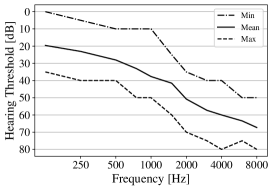
Figure 7: Distribution of the left-right-ear averaged pure-tone audiograms of all subjects. Min denotes the minimal hearing threshold of the TPs, and max denotes the maximum hearing threshold of the TPs. Mean denotes the average hearing threshold of the 13 TPs.

Additionally, the average age of the TPs used for the final listening experiments was 75.5 years, of which eight TPs were biologically male and five were biologically female.

VI-B Testing conditions

The listeners were placed in a soundproof booth, wearing Sennheiser HDA200 headphones. Each signal was always normalized at peak magnitude, thus, to some degree, accounting for loudness differences between the systems, while ensuring there was was no clipping. The volume is personally adjusted by the individual, and we test it across various systems to guarantee that the signals are loud enough to be heard. We ensure the signals surpass the hearing threshold by: 1) assessing their listening skills on the systems using HINT lists not utilized during data collection, and 2) instructing the TP to make the signals ”slightly” loud, gradually increasing the level until the signal is well above the threshold. The volume stays fixed during all of the tests.

In our comparison between DNN-HLC and a conventional HLC, we chose to employ the NAL-R fitting rationale as the conventional HLC. This decision was guided by NAL-R [9] being linear and non-proprietary, making the results easier replicable. While newer WDRC-based strategies like NAL-NL2 [34] have emerged, potentially outperforming NAL-R, it’s essential to note that our study focused on a fixed SPL level. The primary advantage of utilizing the NAL-NL2 fitting rationale lies in its capability to span a broad range of input SPL levels. Under conditions with sufficiently low compression ratios, relatively stationary noise and longer time constants, NAL-NL2 may essentially function as a linear filter at a fixed SPL, resulting in an essentially linear system with a varied gain/frequency curve. Additionally, we compare our joint DNN-HLCNR with a generic DNN-NR, cf. Sec. V. The 5 systems are as follows:

1. Unprocessed

2. NAL-R [9] (prescribed linear gain)

3. DNN-HLC

4. Generic NR followed by NAL-R (defined as NR + NAL-R)

5. DNN-HLCNR (joint HLC and NR)

VI-C Hearing in Noise Test

For the HINT, we wanted to target the steepest part of the psychometric function and therefore generated signals at 0 dB and 3 dB SNR [35] with 16-speaker babble noise. The signals were then processed by all the systems, totaling 10 different conditions. For each subject, each condition was assigned to a random HINT list, of which there were 10 ($2$ SNRs $\times$ $5$ systems). Each HINT list consists of 20 sentences with 5 word in each sentence, and the subjects were instructed to repeat the words they heard. If the subjects were unable to discern any words, they were instructed to say ”pass”. Additionally, the subjects were instructed that guessing were allowed if they were uncertain of some specific word.

VI-D MUSHRA test

For the MUSHRA test, the signals were generated at a SNR of 9 dB - close to perfect intelligibility, so the noise did not confound the MUSHRA score - then processed by each system, except for the Unprocessed condition. Instead of the unprocessed condition, we included a hidden anchor, which was the unprocessed signal at an SNR of 3 dB. The anchor, firstly, provided a lower fixed-point for the 0-100 MUSHRA scale, and secondly, the anchor could be used for detecting subjects that rated the anchor favourably, thus not performing the tests properly. The test signals were the first 15 sentences of the Danish HINT, List 1. For each sentence, each system was given a random number (1 through 5) and the subjects were instructed to rank the systems from the most preferred (100) to the least preferred (0). The subject performed a ranking using a computer-interface with 5 sliders, and a play button for each number (1 through 5). The MUSHRA test is self-paced, and the subject could listen to the five different systems as many times as they would like. Naturally, as we do not have access to a ground truth reference, i.e. a processing of signal that is truly optimal for each individual, for each sentence, we did not include a reference.

VI-E Pilot tests

During the first pilot tests, we found that the DNN-HLC and DNN-HLCNR did not perform very well, particularly at high frequencies, where large tonal components were introduced. Our hypothesis is that this behaviour was caused by the frequency response of the auditory-model channels essentially becoming flat for sufficiently large hearing losses, see Fig. 8. Thus, the output of the DNNs gave too much low frequency amplification and strong, tonal artifacts at high frequencies, where the CFs were not constrained around their peaks. Thus, the goal should be to constrain the loss function to be sensitive to only near-CF behaviour for each channel. In order to circumvent this problem, we experimented with different loss functions, which unfortunately all suffered from the same problem. Thus, we instead opted to reduce the hearing loss in the auditory model, by diving the audiogram with 2, as this directly imposes a near-CF sensitivity constraint on each channel. Additionally, we found that the trained DNNs resulted in gain curves within the same order of magnitude as NAL-R. A comparison of the resulting gain, g, of NAL-R and DNN-HLC is shown for a realistic hearing loss in Fig. 9.

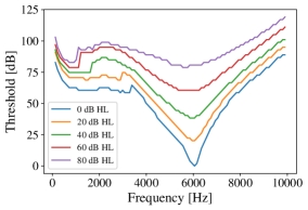
Figure 8: Thresholds at the auditory nerve level, using the Zilany auditory model, at a CF of 6 kHz. The thresholds are calculated, for each frequency, as the level where the mean firing rate is 1 standard deviation larger than spontaneous firing rate.

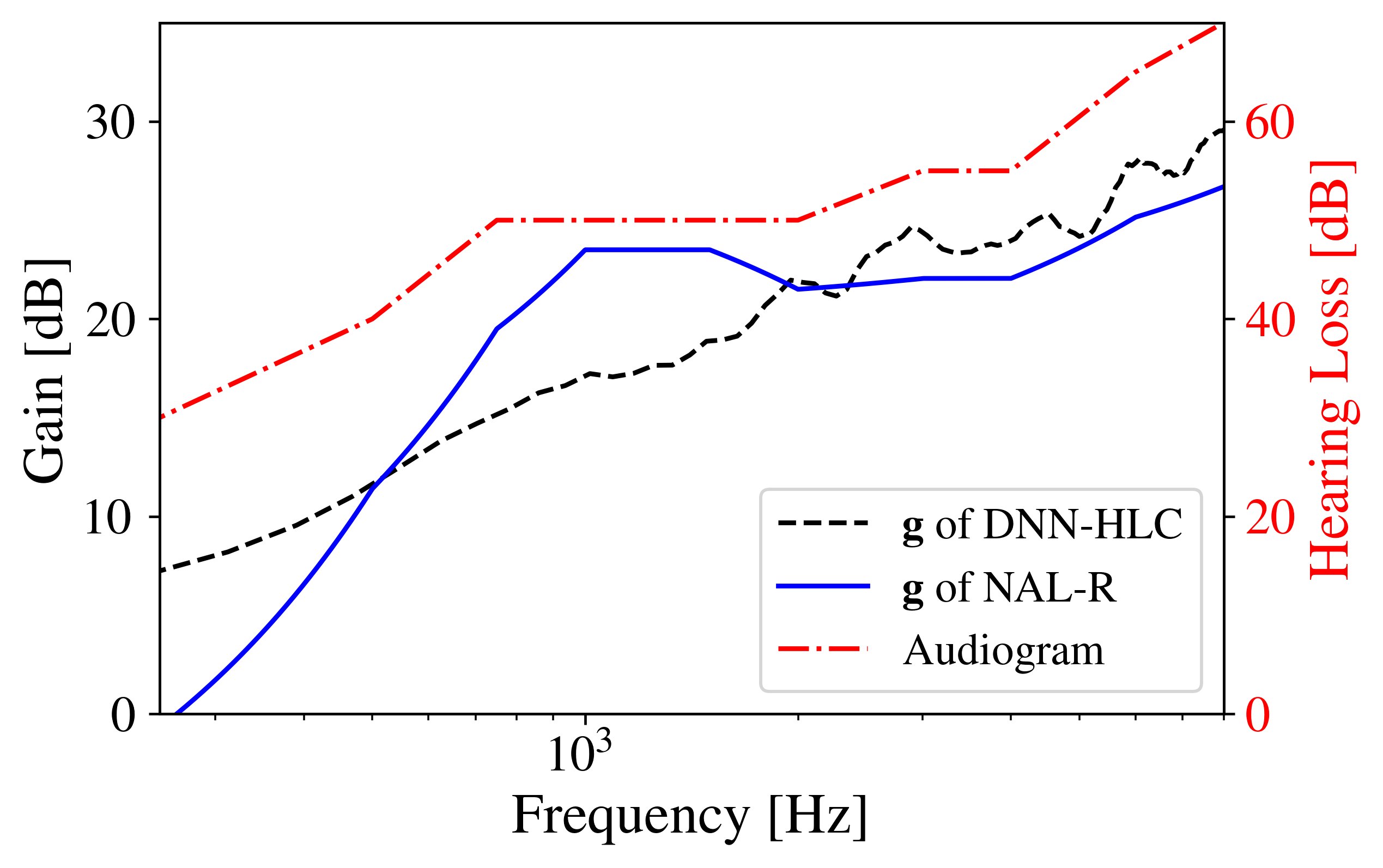
Figure 9: Comparison of g for the linear compensation strategy, NAL-R, and the DNN-based hearing-loss compensation strategy, DNN-HLC.

VII Results

In this section we will present our results from the listening tests, where we measure the performance of our proposed hearing-loss compensation strategies.

VII-A HINT results

Fig. 10 shows the results of the HINT, displayed as a violinplot. By performing a multiple comparison of means using a Tukey’s range test, we found no significant difference between any of the conditions, using a family-wise error rate (FWER) of $\alpha=0.05$. Instead, we fit the data using a linear mixed model (LMM) [36] to model both the random effect of different TPs, and the additive, fixed effect of SNR, using the following formula:

Intelligibility $$\sim C(\text{System, Treatment('Unprocessed')})$$

$$+C(\text{SNR})+\text{Random Effects of TP}+\epsilon$$ (21)

where $\text{C}(\cdot)$ denotes a categorical variable, the Treatment refers to setting the mean of the ”Unprocessed” system as the intercept, and $\epsilon$ as the residuals. Thus, the coefficient of a variable indicates the predicted increase in intelligibility from the unprocessed system.

The results of such a LMM, shown in Table III, indicates that there is a high probability of a significant improvement ($p\approx 0.0003$) using the DNN-HLC, leading to an $11\%$ increased intelligibility, as compared to the unprocessed system. There is evidence ($p\approx 0.02$) that the NR-based systems also provide increased intelligibly. Additionally, there is an indication ($p\approx 0.08$) that NAL-R provides some benefit.

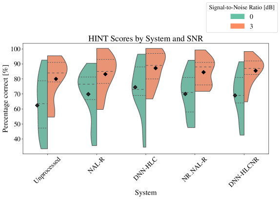
Figure 10: Boxplot of the results for the hearing in noise test (HINT) for the 5 different systems at two different SNRs. The black diamonds denote the mean percentage correct of each condition, and the inner lines are the 1st, 2nd and 3rd quantile.

Variable	Coeff.	Adj. p-value
Intercept (Unprocessed)	62	0
C(NAL-R)	5	0.078
C(DNN-HLC)	11	0.0003
C(NR+NAL-R)	7	0.02
C(DNN-HLCNR)	7	0.02
C(SNR=3)	16	0
Variance of Random effects of TP + $\epsilon$	109	0.039

TABLE III: Coefficients of a Linear Mixed Model fitted to the outcome of the HINT test. The p-values are adjusted using Benjamini-Hochberg correction.

VII-B MUSHRA test

Fig. 11 shows a violin plot of the data collected from the MUSHRA test. A Wilcoxon signed-rank test was performed between all the different systems. All possible comparisons were significant using a FWER of $\alpha=0.05$ after using Benjamini-Hochberg corrections. For easier readability, the average and median score of each system are shown in Table IV, where we find that DNN-HLC is preferred over NAL-R by a small margin, and that the DNN-HLCNR is the most preffered system, with a median score of 94:

System	Mean score	Median score
Anchor	18	14
NAL-R	49	50
DNN-HC	55	51
NR + NAL-R	72	74
DNN-HLCNR	81	94

TABLE IV: Average and median score of the MUSHRA test for each system

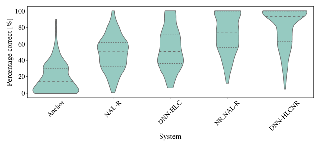
Figure 11: Distribution of the results for the MUHSRA test for 5 different conditions (Anchor, NAL-R, DNN-HLC, NR_NAL-R, DNN-HLCNR), indicating different processing strategies.

VIII Discussion and future works

In the HINT, the intelligibility tests, we found that the DNN-based hearing-loss compensation strategies (DNN-HLC) performed comparably to the joint hearing-loss compensation and noise-reduction strategies (DNN-HLCNR). It is somewhat counter-intuitive that the DNN-HLCNR does not siginificantly outperform the DNN-HLC, and one reason might be that the noise-reduction is known to sometimes generalize poorly to out-of-distribution datasets, particularly when the out-of-distribution dataset does not contain the same speakers as the original training set. [37]. In this work, the DNN-HLCNR was trained on English speakers, meanwhile our test data was from different spakers in a different language, which could be problematic. In the MUSHRA test, that measured percieved quality, the DNN-HLCNR outperformed all other systems, which could be due to a more appropriate compensation for the individual, but alternatively could be due to simply better generalization capabilities due to better convergence behaviour.

Finally, the importance of the temporal non-linear processing of the DNN-HLC - and how it potentially diverges from conventional strategies - versus the long-term frequency shaping of the DNN-HLC should be investigated in future works. In this work, the input sound level was kept fixed at 65 dB SPL - corresponding to normal conversation levels - but everyday sounds will cover a larger range of sound levels. Thus, it still remains to be shown that a DNN like the DNN-HLC can process a large range of input levels, while providing a safe and comfortable listening experience for the hearing impaired person. Future work should investigate how different loss functions interact with specific hearing losses, and what the effects are on the final compensation strategies.

IX Conclusion

In this work we presented a deep-neural-network (DNN) based framework for providing personalized hearing loss compensation (HLC) and noise reduction (NC) strategies using auditory models. An auditory model of the auditory pathway, including an auditory-nerve model was emulated using a DNN, which subsequently was used to train the HLC and NR strategies. The HLC strategy was analyzed using a simple, linearized model, which showed that some of the linear effects of the DNN-based hearing-loss compensation strategy can be predicted before training the DNN, which might assist in hyperparameter choices of the auditory model, e.g. spacing of center frequencies of the auditory model. Finally, the derived HLC and NR strategies were evaluated in terms of intelligibility and perceived quality and compared to conventional signal-processing strategies. In terms of intelligibility in a difficult listening scenario, the listening experiments showed that resulting DNN-based HLC and NR strategies outperformed a baseline consisting of unprocessed signals. In particular a linear mixed model showed that the DNN-based HLC strategy outperformed the conventional HLC strategy. In terms of speech quality, the proposed joint HLC and NR outperformed a generic NR, followed by a conventional HLC strategy. Although the results are promising, several issues remain to be addressed, such as generalization to unseen types of noise, languages and speakers, characterization and explanation of the DNN-based hearing-loss compensation strategies and insuring stability and performance across a wide range of inputs.

References

- [1] Rasiah and Sulakshan, “Addressing the rising prevalence of hearing loss,” World Health Organization, 2018.
- [2] P. Leer, J. Jensen, Z.-H. Tan, J. Østergaard, and L. Bramsløw, “How to train your ears: Auditory-model emulation for large-dynamic-range inputs and mild-to-severe hearing losses,” In press.
- [3] E. Biondi, “Auditory processing of speech and its implications with respect to prosthetic rehabilitation. The bioengineering viewpoint,” International Journal of Audiology, vol. 17, no. 1, pp. 43–50, 1978.
- [4] J. Bondy, S. Becker, I. Bruce, L. Trainor, and S. Haykin, “A novel signal-processing strategy for hearing-aid design: Neurocompensation,” Signal Processing, vol. 84, no. 7, pp. 1239–1253, 2004.
- [5] Z. Chen, S. Becker, J. Bondy, I. C. Bruce, and S. Haykin, “A Novel Model-Based Hearing Compensation Design Using a Gradient-Free Optimization Method,” Neural Computation, vol. 17, no. 12, pp. 2648–2671, 12 2005. [Online]. Available: https://dx.doi.org/10.1162/089976605774320575
- [6] P. v. Hengel, “Simulating hearing loss with a transmission-line model for the optimization of hearing aids,” Proceedings of the International Symposium on Auditory and Audiological Research, vol. 5, pp. 181–188, 12 2015. [Online]. Available: https://proceedings.isaar.eu/index.php/isaarproc/article/view/2015-21
- [7] F. Drakopoulos and S. Verhulst, “A Neural-Network Framework for the Design of Individualised Hearing-Loss Compensation,” IEEE/ACM Transactions on Audio Speech and Language Processing, vol. 31, pp. 2395–2409, 2023.
- [8] C. V. Palmer and G. A. Lindley Iv, “Overview And Rationale For Prescriptive Formulas for Linear and Non-Linear Hearing Aids,” in Strategies for Selecting and Verifying Hearing Aid Fittings., P. Michael Valente, Ed. Thieme Medical Publishers, 2002, pp. 1–22. [Online]. Available: https://web.thieme.com/media/samples/pubid1013629716/
- [9] D. Byrne and H. Dillon, “The National Acoustic Laboratories’ (NAL) new procedure for selecting the gain and frequency response of a hearing aid,” Ear and hearing, vol. 7, no. 4, pp. 257–265, 1986. [Online]. Available: https://pubmed.ncbi.nlm.nih.gov/3743918/
- [10] G. A. Lindley IV and C. V. Palmer, “Fitting Wide Dynamic Range Compression Hearing Aids,” American Journal of Audiology, vol. 6, no. 3, pp. 19–28, 1997. [Online]. Available: https://pubs.asha.org/doi/10.1044/1059-0889.0603.19
- [11] N. Le Goff, “Amplifying soft sounds-a personal matter,” 2014. [Online]. Available: https://www.oticon.global/professionals/audiology-and-technology/technologies/research
- [12] T. Schneider and R. Brennan, “Multichannel compression strategy for a digital hearing aid,” ICASSP, IEEE International Conference on Acoustics, Speech and Signal Processing - Proceedings, vol. 1, pp. 411–414, 1997.
- [13] J. M. Kates and K. H. Arehart, “Multichannel dynamic-range compression using digital frequency warping,” Eurasip Journal on Applied Signal Processing, vol. 2005, no. 18, pp. 3003–3014, 2005. [Online]. Available: https://www.researchgate.net/publication/26532062_Multichannel_Dynamic-Range_Compression_Using_Digital_Frequency_Warping
- [14] M. S. A. Zilany, I. C. Bruce, and L. H. Carney, “Updated parameters and expanded simulation options for a model of the auditory periphery,” The Journal of the Acoustical Society of America, 2014.
- [15] S. Verhulst, A. Altoè, and V. Vasilkov, “Computational modeling of the human auditory periphery: Auditory-nerve responses, evoked potentials and hearing loss,” Hearing Research, vol. 360, pp. 55–75, 2018.
- [16] “Auditory Models - Publications - Carney Lab - University of Rochester Medical Center.” [Online]. Available: https://www.urmc.rochester.edu/labs/carney/publications-code/auditory-models.aspx
- [17] M. S. A. Zilany, I. C. Bruce, P. C. Nelson, and L. H. Carney, “A phenomenological model of the synapse between the inner hair cell and auditory nerve: Long-term adaptation with power-law dynamics,” The Journal of the Acoustical Society of America, vol. 126, no. 5, pp. 2390–2412, 11 2009. [Online]. Available: https://www.researchgate.net/publication/38072230_A_phenomenological_model_of_the_synapse_between_the_inner_hair_cell_and_auditory_nerve_Long-term_adaptation_with_power-law_dynamics
- [18] “GitHub - HearingTechnology/CoNNear_cochlea.” [Online]. Available: https://github.com/HearingTechnology/CoNNear_cochlea
- [19] H. Zen, V. Dang, R. Clark, Y. Zhang, R. J. Weiss, Y. Jia, Z. Chen, and Y. Wu, “LibriTTS: A Corpus Derived from LibriSpeech for Text-to-Speech,” Proceedings of the Annual Conference of the International Speech Communication Association, INTERSPEECH, vol. 2019-September, pp. 1526–1530, 4 2019. [Online]. Available: https://arxiv.org/abs/1904.02882v1
- [20] N. Rahaman, A. Baratin, D. Arpit, F. Draxlcr, M. Lin, F. A. Hamprecht, Y. Bengio, and A. Courville, “On the Spectral Bias of Neural Networks,” 36th International Conference on Machine Learning, ICML 2019, vol. 2019-June, pp. 9230–9239, 6 2018. [Online]. Available: https://arxiv.org/abs/1806.08734v3
- [21] K. He, X. Zhang, S. Ren, and J. Sun, “Delving deep into rectifiers: Surpassing human-level performance on imagenet classification,” Proceedings of the IEEE International Conference on Computer Vision, vol. 2015 Inter, pp. 1026–1034, 2015.
- [22] K. Hornik, M. Stinchcombe, and H. White, “Multilayer feedforward networks are universal approximators,” Neural Networks, vol. 2, no. 5, pp. 359–366, 1 1989.
- [23] P. D. Welch, “The Use of Fast Fourier Transform for the Estimation of Power Spectra,” IEEE Transactions on audio and electroacoustics, no. 2, pp. 70–73, 1967.
- [24] F. Drakopoulos, A. Van Den Broucke, and S. Verhulst, “A DNN-Based Hearing-Aid Strategy For Real-Time Processing: One Size Fits All,” ICASSP, IEEE International Conference on Acoustics, Speech and Signal Processing - Proceedings, pp. 1–5, 5 2023.
- [25] C. M. Bishop, Pattern Recoginiton and Machine Learning. Springer-Verlag New York, 2006.
- [26] N. Bisgaard, M. S. Vlaming, and M. Dahlquist, “Standard Audiograms for the IEC 60118-15 Measurement Procedure,” Trends in Amplification, vol. 14, no. 2, pp. 113–120, 2010. [Online]. Available: http://tia.sagepub.com
- [27] D. Stoller, S. Ewert, and S. Dixon, “Wave-U-Net: A multi-scale neural network for end-to-end audio source separation,” Proceedings of the 19th International Society for Music Information Retrieval Conference, ISMIR 2018, pp. 334–340, 2018.
- [28] Y. Luo and N. Mesgarani, “Conv-TasNet: Surpassing Ideal Time-Frequency Magnitude Masking for Speech Separation,” IEEE/ACM Transactions on Audio Speech and Language Processing, vol. 27, no. 8, pp. 1256–1266, 9 2018. [Online]. Available: http://arxiv.org/abs/1809.07454http://dx.doi.org/10.1109/TASLP.2019.2915167
- [29] E. Tzinis, Z. Wang, and P. Smaragdis, “Sudo rm -rf: Efficient Networks for Universal Audio Source Separation,” IEEE International Workshop on Machine Learning for Signal Processing, MLSP, vol. 2020-September, 7 2020. [Online]. Available: http://arxiv.org/abs/2007.06833http://dx.doi.org/10.1109/MLSP49062.2020.9231900
- [30] M. Kolbaek, Z. H. Tan, S. H. Jensen, and J. Jensen, “On Loss Functions for Supervised Monaural Time-Domain Speech Enhancement,” IEEE/ACM Transactions on Audio Speech and Language Processing, vol. 28, pp. 825–838, 2020.
- [31] J. L. Roux, S. Wisdom, H. Erdogan, and J. R. Hershey, “SDR - half-baked or well done?” ICASSP, IEEE International Conference on Acoustics, Speech and Signal Processing - Proceedings, vol. 2019-May, pp. 626–630, 11 2018. [Online]. Available: https://arxiv.org/abs/1811.02508v1
- [32] J. B. Nielsen and T. Dau, “The Danish hearing in noise test,” International Journal of Audiology, vol. 50, no. 3, pp. 202–208, 3 2011. [Online]. Available: https://www.tandfonline.com/doi/abs/10.3109/14992027.2010.524254
- [33] I. Radiocommunication Sector, “Method for the subjective assessment of intermediate quality level of audio systems BS Series Broadcasting service (sound),” 2015. [Online]. Available: http://www.itu.int/ITU-R/go/patents/en
- [34] G. Keidser, H. Dillon, M. Flax, T. Ching, and S. Brewer, “The NAL-NL2 Prescription Procedure,” Audiology Research, vol. 1, no. 1, 2011.
- [35] J. B. Nielsen, Assessment of speech intelligibility in background noise and reverberation, 2009.
- [36] A. S. Bryk and S. W. Raudenbush, Hierarchical linear models: Applications and data analysis methods. Advanced quantitative techniques in the social sciences. SAGE Publications, 1992.
- [37] P. Gonzalez, T. S. Alstrøm, and T. May, “Assessing the Generalization Gap of Learning-Based Speech Enhancement Systems in Noisy and Reverberant Environments,” IEEE/ACM Transactions on Audio, Speech, and Language Processing, 2023.