Collaborative Aquatic Positioning System Utilising Multi-beam Sonar and Depth Sensors

Abstract

Accurate positioning of remotely operated underwater vehicles (ROVs) in confined environments is crucial for inspection and mapping tasks and is also a prerequisite for autonomous operations. Presently, there are no positioning systems available that are suited for real-world use in confined underwater environments, unconstrained by environmental lighting and water turbidity levels and have sufficient accuracy for long-term, reliable and repeatable navigation. This shortage presents a significant barrier to enhancing the capabilities of ROVs in such scenarios. This paper introduces an innovative positioning system for ROVs operating in confined, cluttered underwater settings, achieved through the collaboration of an omnidirectional surface vehicle and an ROV. A formulation is proposed and evaluated in the simulation against ground truth. The experimental results from the simulation form a proof of principle of the proposed system and also demonstrate its deployability. Unlike many previous approaches, the system does not rely on fixed infrastructure or tracking of features in the environment and can cover large enclosed areas without additional equipment.

I Introduction

I-A Motivation

Over the past few decades, the domain of underwater robotics has experienced considerable expansion. Presently, the use of Remotely Operated Vehicles (ROVs) has become safe and routine, not only within the offshore industry, but also in confined aquatic environments. Numerous examples can be found in the literature, such as pipeline inspection [1], monitoring of nuclear storage facilities [2] and liquid storage tank inspections [3]. Safety concerns and cost-effectiveness are the primary motivations behind this transition from human divers to ROVs [4]. However, navigating underwater vehicles through confined and sometimes cluttered environments is challenging. Precision movement is crucial in these environments, as vehicles must navigate through narrow passages and avoid obstacles [5].

Presently most ROV missions in confined underwater environments are teleoperated [6]. However, there are several benefits to performing fully autonomous missions, including cost reduction, repeatability, and increased survey frequency [7]. Even lower levels of autonomy, such as position and velocity control, can facilitate smooth and accurate navigation or fixing sensor position or velocity for accurate surveying. To achieve autonomy, accurate positioning is essential [6] and currently there are no positioning systems available that are practical for use in confined underwater environments (as discussed in Section II-A). In addition to facilitating autonomy, location-tagged sensor data can be used for long-term environmental monitoring and analysis. In a recent study [8] published from the Fukushima Daiichi Nuclear Power Station in Japan, an investigation was conducted into the environmental conditions of an underground facility used for the temporary storage of contaminated water. Hundreds of sandbags filled with zeolite particles were deployed on the floor to remove radioactivity from the water, with plans for future decommissioning using a zeolite removal robot. The positioning of underwater robots contributed to a more precise survey of the underwater environment and facilitated 3D reconstruction. However, in the current stage of deployment, robots have not addressed the issue of underwater localisation to achieve automation; instead, they are controlled through human intervention.

To be useful in practical situations, a confined space localisation system should require minimal infrastructure, meaning that it should not rely on preinstalled cameras, beacons or sensors. Fixing infrastructure in the environment is time consuming, expensive and generally requires calibration. In addition, installing infrastructure is often not practical. For example, in a nuclear spent fuel pool, where access is highly restricted for safety reasons, it would be impractical to install beacons or other infrastructure around the pool.

In this work, a Collaborative Aquatic Positioning (CAP) system is proposed that aims to satisfy the requirements stated above. Given the prevalent conditions of insufficient illumination and high turbidity in many underwater environments, the proposed localisation system abandons the use of traditional optical cameras for tracking and instead employs multi-beam sonar. The proposed system uses an autonomous surface vehicle (ASV) that can self localise relative to the walls. The surface vehicle tracks and remains above the underwater ROV. By combining sensor measurements from both vehicles, the pose of the subsurface vehicle can be determined. This system requires no fixed infrastructure and minimal calibration. In the next section a review of related underwater localisation systems is provided.

I-B Contribution

The main contributions of this paper are as follows:

1. A novel formulation of a collaborative underwater positioning system that is suited for use in real world ROV missions in confined environments and, unlike previous systems with comparable accuracy, does not require any fixed infrastructure, does not rely on tracking environmental, can cover large areas and operate in highly turbid water with no lighting requirements.

2. Simulation proof of principle demonstrates the correctness of the proposed CAP-SD mathematical model, showing that the positioning system possesses an acceptable level of accuracy for a variety of applications.

II Related work

II-A Literature review

II-A1 ACOUSTIC TRANSPONDERS AND BEACONS

This method includes long baseline (LBL), short baseline (SBL) and ultra short baseline (USBL) systems and is primarily designed for use in open oceans. Baseline localisation is accomplished by measuring distances between transponders and beacons based on the time-of-flight of acoustic signals. Regarding legacy acoustic positioning systems (APS), there are primarily two types: those developed as a result of academic research and those that are commercialised products. In academic research, APS is often integrated with other positioning technologies, such as Doppler Velocity Loggers (DVL) and inertial sensors. In [9], field experiments have demonstrated that for these technologies, the positioning error exceeds 1 meter for the majority of the time. The experimental validation of a tightly coupled USBL and inertial navigation system proposed in [10] also indicates a root mean square estimation error (RMSE) in position ranging between 1 and 2 meters. In commercial APS,  [11] is among the most precise and is typically integrated into medium and small-sized underwater robots, offering positioning accuracy within 0.1 meters for distances up to 5 meters.

However, regardless of the type, all USBL systems require infrastructure in the form of fixed transponders to be located in the environment, and require sophisticated calibration or input from GNSS, which is often unavailable in enclosed environments.

II-A2 SIMULTANEOUS LOCALISATION AND MAPPING

Simultaneous localization and mapping (SLAM) is a widely researched topic in the field of robotics for ground and aerial vehicles. However, underwater SLAM is more challenging due to the fact that commonly used sensors such as cameras and LiDARs do not perform well underwater due to higher photon absorption. In [12], Rahman et al. validated three visual SLAM techniques underwater, OKVIS (Stereo) [13], VINS-Mono [14] and ORB-SLAM3 (Stereo-in) [15]. These visual SLAM algorithms can provide localisation with reasonable accuracy: RMSE 0.1-0.3 m. However, visual SLAM needs to constantly identify features in the image to provide accurate positioning, which can be problematic underwater, where visibility is lower than in air and environments are often feature sparse.

Sonar SLAM in an underwater environment is analogous to 2D LiDAR based SLAM in a terrestrial environment [16]. Testing in an abandoned marina, Mallios et al. found that their pose-based SLAM method had a mean accuracy of 1.9 m [17], which, even if this could be repeated in a confined environment, is too high to be of use in many applications.

II-A3 FIXED INFRASTRUCTURE CAMERA TRACKING SYSTEMS

Duecker et al. [18] placed an array of 63 fiducial markers around the perimeter of a tank and used a vehicle mounted camera combined with AprilTag tracking to estimate the pose of the camera in the tank, achieving an RMSE of 2.6 cm. Other systems, such as the Qualisys Miqus, use fixed cameras to track markers that are attached to the ROV and can return sub centimetre accuracy [19]. Despite their high accuracy, camera tracking systems with fixed infrastructure are generally only useful in lab settings, as they have significant setup and access requirements and limited volume coverage. Furthermore, since such methods primarily utilize optical cameras, they become unsuitable in underwater environments with low ambient illumination levels and high turbidity.

II-A4 DEAD RECKONING

Dead reckoning estimates current position based on a previously known or estimated position, using direction and distance traveled. Pure dead reckoning uses exclusively ROV mounted sensors and requires no infrastructure. There are two key technologies that are typically used for underwater dead reckoning: Doppler Velocity Logs (DVLs) [20] and inertial measurement units (IMUs) [21]; these two technologies are commonly combined [22]. However, due to the nature of the method, all dead reckoning systems accumulate errors [23] and are therefore most commonly used to aid other systems that can directly provide position relative to the environment or fixed infrastructure. In [24], an IMU based nonlinear observer for dead reckoning was proposed. It was demonstrated the RMSE of the system was 100 meters after 10 minutes.

II-A5 SUMMARY

It is apparent that although individual technologies meet some of the requirements detailed in Section I-A, none of the technologies reviewed are sufficient to meet the combination of requirements. From a technical perspective, relying solely on multi-beam sonar is insufficient for determining the three-dimensional coordinates of an object [25] [26]. These motivate the development of the CAP system presented in this paper, which integrates a multi-beam sonar and depth sensor (CAP-SD).

III CAP-SD formulation

III-A Notations and coordinate frames

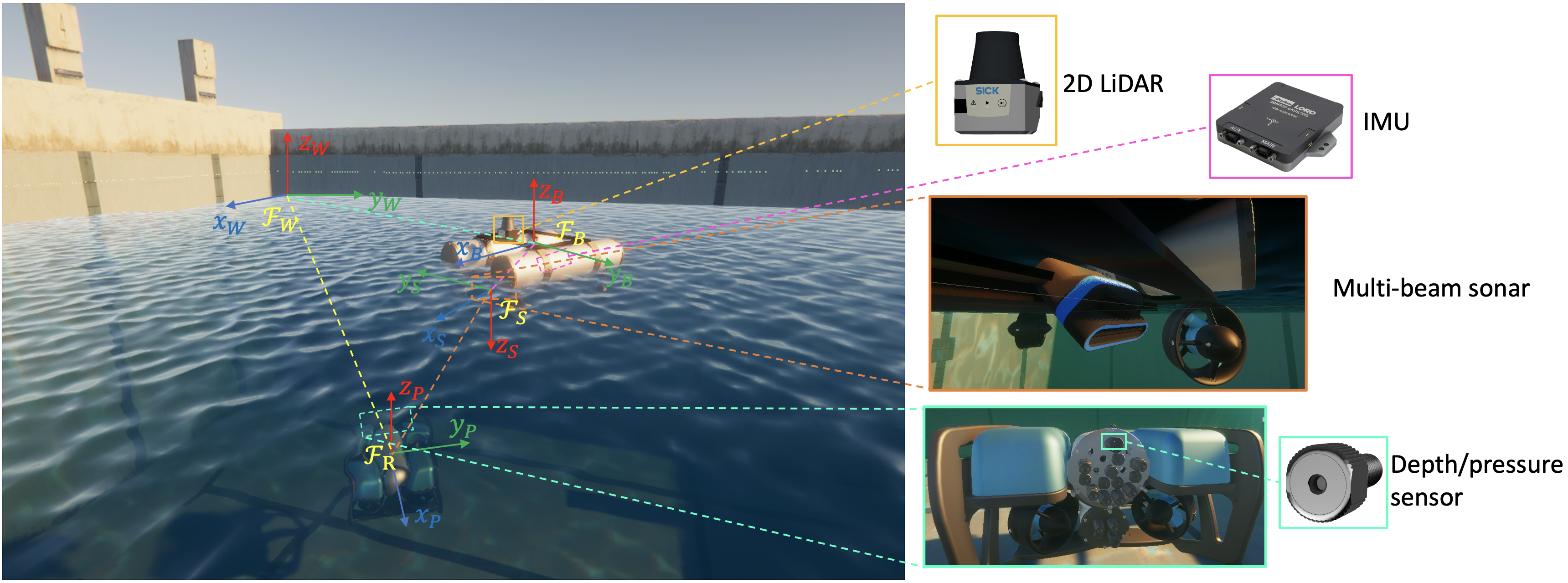
Figure 1: Overview of the components and coordinate frames of the confined aquatic positioning (CAP-SD) system. An omnidirectional ASV - MallARD, with integrated LiDAR, IMU, and an image sonar tracks a submersible ROV. The ROV is also fitted with a pressure sensor for depth measurement.

Figure 1 presents the coordinate system and reference frames used in this work. The full positioning system is composed of the following co-ordinate frames: the inertial world frame $\mathcal{F}_{W}$, ASV baselink frame $\mathcal{F}_{B}$, multi-beam sonar $\mathcal{F}_{S}$ and ROV frame $\mathcal{F}_{R}$. The world frame $\mathcal{F}_{W}$ origin is assigned to a corner of the testing tank. $\mathcal{F}_{B}$ is the geometric centre of the ASV. The origin of the sonar frame $\mathcal{F}_{S}$ is located at the optical center of the transmitter and has a static transform from $\mathcal{F}_{B}$.

The transformation from one arbitrary coordinate frame $\mathcal{F}_{A}$ to another $\mathcal{F}_{B}$ can be expressed as a homogeneous transformation matrix:

$$\mathbf{H}^{A}_{B}=\left[\begin{array}[]{cc}\mathbf{R}^{A}_{B}&\mathbf{p}^{A}_{B}\\ 0&1\end{array}\right]$$ (1)

where $\mathbf{R}^{A}_{B}\in\mathrm{SO}(3)$ is a rotation matrix from frame A to frame B and $\mathbf{p}^{A}_{B}\in\mathbb{R}^{3}$ is translation column vector. $\mathbf{H}\in SE(3)$ represents the combination of rotation and translation in three dimensions, which can also be expressed as the pair $[\mathbf{R},\mathbf{p}]$.

III-B CAP-SD formulation overview

The full transform chain from the world frame $\mathcal{F}_{W}$ to the ROV frame $\mathcal{F}_{R}$:

$$\mathbf{H}_{S}^{W}=\mathbf{H}_{B}^{W}\mathbf{H}_{S}^{B}\mathbf{H}^{S}_{R},$$ (2)

can not be used to obtain $\mathbf{P}^{W}_{R}=[x^{W}_{R},y^{W}_{R},z^{W}_{R}]^{\top}$ directly because $\mathbf{P}^{S}_{R}$ cannot be defined. This is because the multi-beam sonar generates 2-D visualisations of the 3-D environment, where each pixel in the image represents an arc in 3D space, originating from the center of the multi-beam sonar.

In this scenario, each pixel has a direct correlation with both the azimuth angle ($\theta$) and the distance (R) of the arc from its origin, but the aggregation of spatial returns along these arcs precludes the retrieval of elevation angles ($\phi$), as shown in Figure 2A. Therefore, even if the location of the ROV is successfully identified in the sonar’s scan, the translation $\mathbf{P}^{S}_{R}=[x^{S}_{R},y^{S}_{R},z^{S}_{R}]^{\top}$ can not be defined and the transform chain is incomplete. To resolve this problem, the CAP-SD system uses the available elements of the transform chain and the pixel location of the ROV in the sonars image to generate an arc of possible positions of the ROV in the world frame $\mathcal{F}_{W}$. A pressure sensor on the ROV is used to generate a horizontal plane (depth plane) of possible robot locations in $\mathcal{F}_{W}$. By finding the intersection of the arc and the horizontal plane, a single location for the ROV in  $\mathcal{F}_{W}$ can be ascertained.

III-C CAP-SD formulation details

First, the pose of the sonar with respect to world-fixed frame ($\mathcal{F}_{W}$), which also serves as the arc’s center, can be expressed by:

$$\mathbf{H}_{S}^{W}=\mathbf{H}_{B}^{W}\mathbf{H}_{S}^{B},$$ (3)

where $\mathbf{H}_{S}^{B}$ is a static homogenous transformation from ASV’s baselink frame to sonar frame and $\mathbf{H}_{B}^{W}$ is detailed in Section III-E.

Second, the pixel location of the ROV in the sonar scan is identified using an object detection neural network. The pixel location in the sonar image is used to determine the distance from the sonar to the ROV R and the angle $\theta$, as detailed in Section III-D..

Third, the arc, represented by a circle in 3D space, is defined. This involves first defining a sphere of possible locations and then defining a sphere-cutting plane, where the intersection between the sphere and the sphere-cutting plane defines the circle. The centre of the sphere is the origin of $\mathcal{F}_{S}$ and it’s radius is $R$. The sphere is defined as:

$$\left(x-x_{S}^{W}\right)^{2}+\left(y-y_{S}^{W}\right)^{2}+\left(z-z_{S}^{W}\right)^{2}=R^{2},$$ (4)

where $[x_{S}^{W}y_{S}^{W}z_{S}^{W}]^{\top}$ is the position of multi-beam sonar. The sphere-cutting plane can be defined by taking the plane of the $x-z$ axes of $\mathcal{F}_{S}$ and rotating it by the angle $\theta$ about the $y$ axis of $\mathcal{F}_{S}$ (gray plane depicted in Figure 2B). The sphere-cutting plane containing the arc can be represented as:

$$A\left(x-x^{W}_{S}\right)+B\left(y-y^{W}_{S}\right)+C\left(z-z^{W}_{S}\right)=0,$$ (5)

where $\vec{\mathbf{n}}_{3\times 1}=[A,B,C]^{\top}$ is the normal vector to the cutting-sphere plane, defined as:

$$\left[\begin{array}[]{c}\vec{\mathbf{n}}_{3\times 1}\\ 1\end{array}\right]=(H^{W}_{B}H^{B}_{S})^{\prime}\left[\begin{array}[]{c}\sin(\theta)\\ -\cos(\theta)\\ 0\\ 1\end{array}\right].$$ (6)

Fourth, the depth plane in $\mathcal{F}_{W}$ must be defined. This is achieved by attaching a pressure sensor to the ROV and calibrating it to measure depth below the surface. The depth plane, which is normal to the $\mathcal{F}_{W}$ $z$-axis, can be defined as:

$$z=z_{depth}.$$ (7)

where $z_{depth}$ is the depth measured by the pressure sensor.

Fifth, by intersecting the sphere, sphere-cutting plane, and the depth plane, the solution domain can be reduced to two points in $\mathcal{F}_{W}$. This is achieve by solving equations (4), (5) and (7) for $x,y$ and $z$.

The final step is to ascertain which of the two points is the correct one. This is relatively simple as the correct solution lies in the positive $x$ region in $\mathcal{F}_{S}$, as shown orange arc in Figure 2C). When transformed into the world-fixed frame, the $x^{W}_{R}$ and $y^{W}_{R}$ must satisfy the following condition:

$$R_{11}x^{W}_{R}+R_{12}y^{W}_{R}+R_{13}z^{W}_{R}+t_{x}>0,$$ (8)

where $R_{11}$, $R_{12}$, $R_{13}$ and $t_{x}$ are elements of the transform:

$$H^{W}_{S}=\left(\begin{array}[]{cccc}R_{11}&R_{12}&R_{13}&t_{x}\\ R_{21}&R_{22}&R_{23}&t_{y}\\ R_{31}&R_{32}&R_{33}&t_{z}\\ 0&0&0&1\\ \end{array}\right).$$ (9)

Therefore, a single point is ultimately identified, which represents the robot’s position $\mathbf{P}^{W}_{R}=[x^{W}_{R},y^{W}_{R},z^{W}_{R}]^{\top}$ with respect of the world-fixed coordinate frame $\mathcal{F}_{W}$.

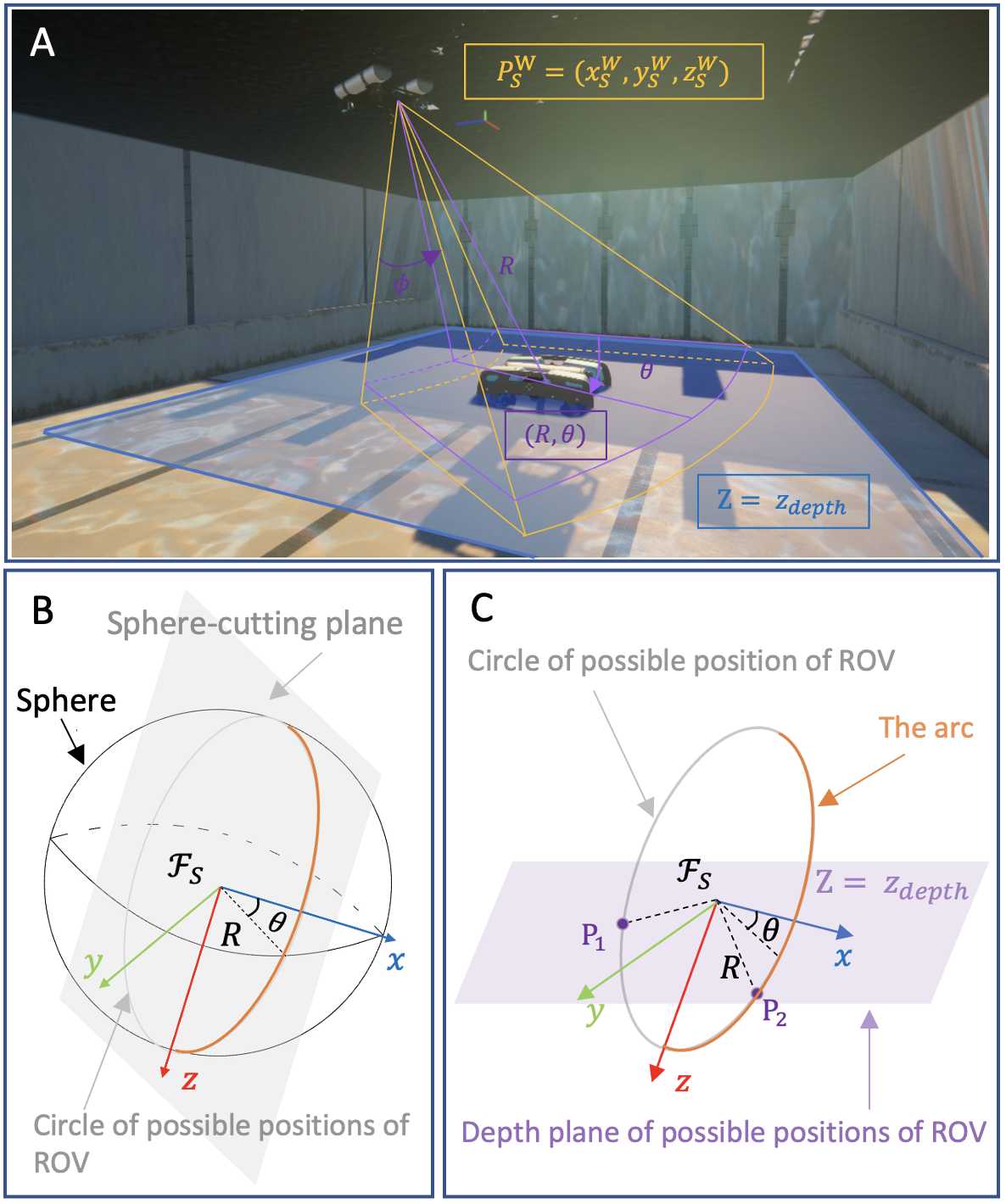
Figure 2: Abstract frames of the CAP-SD system. (A) Underwater side-view of CAP-SD system. (B) Using the cutting-sphere plane and sphere to define the arc where the ROV may be located. (C) Possible locations of ROV can be reduced to two points ($P_{1}$ and $P_{2}$) by generating another plane using the depth sensor. The position of ROV ($P_{2}$) must be in the sonars positive x region (orange arc in (B) and (C)).

III-D Neural network (NN) for image sonar object detection

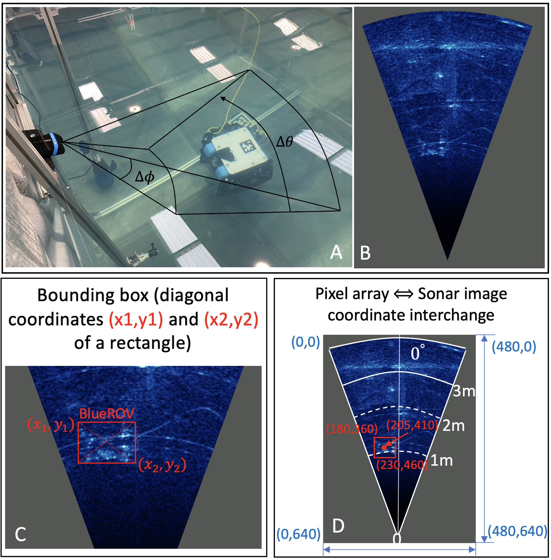
Figure 3: NN object detector (A) Side view of a working scenario involving multi-beam sonar (B)  Raw sonar image (C) Sonar image within NN object detector (D) Pixel array and sonar image coordinate interchange

A high-frequency multi-beam FS sonar emits beams with a fixed vertical width defined by $\left\{\phi_{\min},\phi_{\max}\right\}$ across various azimuth directions $\theta$. In the imaging of the multi-beam sonar, it is displayed as shown in Fig 3A.

The NN detector serves to pinpoint the robot’s pixel coordinates within the sonar image. Given the predefined horizontal field-of-view (FOV), maximum range, and image resolution of an actual multi-beam sonar, determining the robot’s pixel coordinates in the sonar image consequently specifies its distance $R$ and azimuth angle $\theta$ in relation to the multi-beam sonar.

A pre-trained YOLOv5 model  was employed to detect robots in sonar images, which is does by identifying them within bounding boxes as shown in Fig 3C. YOLOv5 builds on the previous YOLO version, with improvements introduced to further boost performance and flexibility to ease deployability in real-world experiments. The pixel coordinates of the robot are obtained at this stage. Subsequently, a conversion from pixel coordinates to sonar image coordinates is performed, as depicted in Fig 3D. For the sonar image frame, its coordinate parameters, such as range and vertical width, are predetermined and fixed. Therefore, pixel coordinates can be directly converted into the sonar image’s $\left\{R,\theta\right\}$ coordinates.

III-E Calculating ASV rotation relative to the world frame $\mathbf{R}^{W}_{B}$

To localise the surface robot within the world-fixed frame, a homogeneous transformation, $\mathbf{H}^{W}_{B}=[\mathbf{R}^{W}_{B},\mathbf{p}^{W}_{B}]$, is calculated. Utilizing a tilting extended Kalman filter (EKF), IMU and SLAM data are fused to estimate the Unmanned Surface Vehicle’s (USV) orientation, $\mathbf{R}^{W}_{B}$. This process incorporates tilt angles from the IMU and the yaw angle from SLAM, adopting a Z-Y-X Euler sequence for the comprehensive rotation matrix construction. Despite Euler angles’ susceptibility to gimbal lock, such occurrences are mitigated here by ensuring the $y$-axis rotation does not exceed 90 degrees, a condition met by surface vehicles.

The EKF is used to accurately estimate pitch and roll angles ($\psi^{W}_{B},\theta^{W}_{B}$) under dynamic conditions, utilizing data from a three-axis gyroscope and accelerometer. Inputs to the tilting EKF include tri-axial angular rates, $\boldsymbol{\omega}=[{\omega}_{x},{\omega}_{y},{\omega}_{z}]^{\top}$, and accelerations, $\boldsymbol{a}=[{a}_{x},{a}_{y},{a}_{z}]^{\top}$, from the USV’s gyroscope and accelerometer, respectively, with the assumption of uncorrelated Gaussian noise. The model assumes negligible non-gravitational linear accelerations during the USV’s motion.

The position and orientation data $[x^{W}_{B},y^{W}_{B},\psi^{W}_{B}]^{\top}$ provided by SLAM (Hector SLAM [27] was deployed on the ASV in the simulation) is notably accurate, as verified by our prior research [28]. The fusion of SLAM and IMU data results in Euler angles $[\psi^{W}_{B},\theta^{W}_{B},\phi^{W}_{B}]^{\top}$, with pitch ($\theta$) and roll ($\phi$) derived from the tilting EKF. Consequently, the rotation matrix $\mathbf{R}^{W}_{B}$ is formulated using the conventional Z-Y-X Euler angles based on the fused orientation data.

IV Results and evaluation

IV-A Simulation architecture

The CAP-SD system underwent evaluation within a custom Unity [29] underwater simulation environment. Portions of the simulation, such as sensors and communication framework, utilized MARUS [30], while the hydrodynamics components for ASVs and AUVs were implemented using the Dynamic Water Physics [31] asset in Unity.

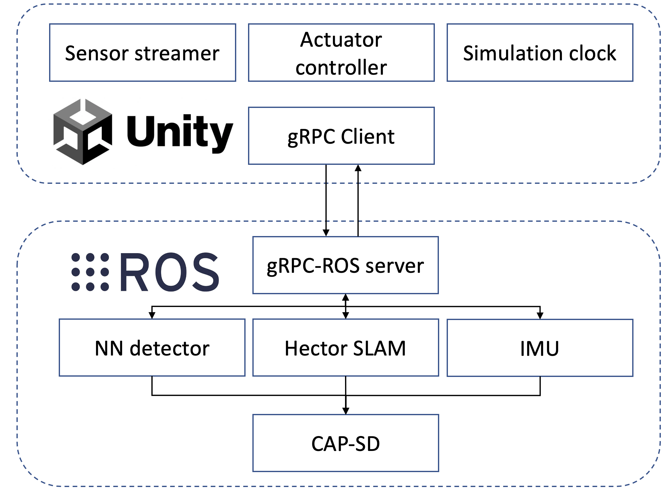
Figure 4: CAP-SD simulation communication architecture

The simulation stack, which incorporates a ROS backend, is depicted in Fig 4. On the ROS [32] side, a gRPC server endpoint is established, functioning as a ROS node responsible for the bidirectional distribution of data flow. On MARUS side (Unity), it obtains inputs for actuators, mission control variables, and requests for simulating communication (either optical or acoustic) within the simulated environment from ROS.

IV-B Simulation Experiment Scenario

Given that the application scenario of CAP-SD will be confined to indoor environments, the simulation scenario is set within a typical nuclear fuel pool (NFP). The entire area measures 28 m in length, 16 m in width, and has a depth of 8 m, as depicted in Fig 3 A and B. Within the NFP, the MallARD [28] (shown in Fig 3C and D), an ASV developed by the University of Manchester and equipped with simulated multi-beam sonar, IMU, and LiDAR, is utilized alongside the commercially available BlueROV2 (shown in Fig 3E and F), which serves as the underwater robot that is to be positioned. This strategic selection is aimed at facilitating the transition of CAP-SD from simulation to real-world deployment. It also lays the foundation for advancing technologies associated with underwater digital twins.

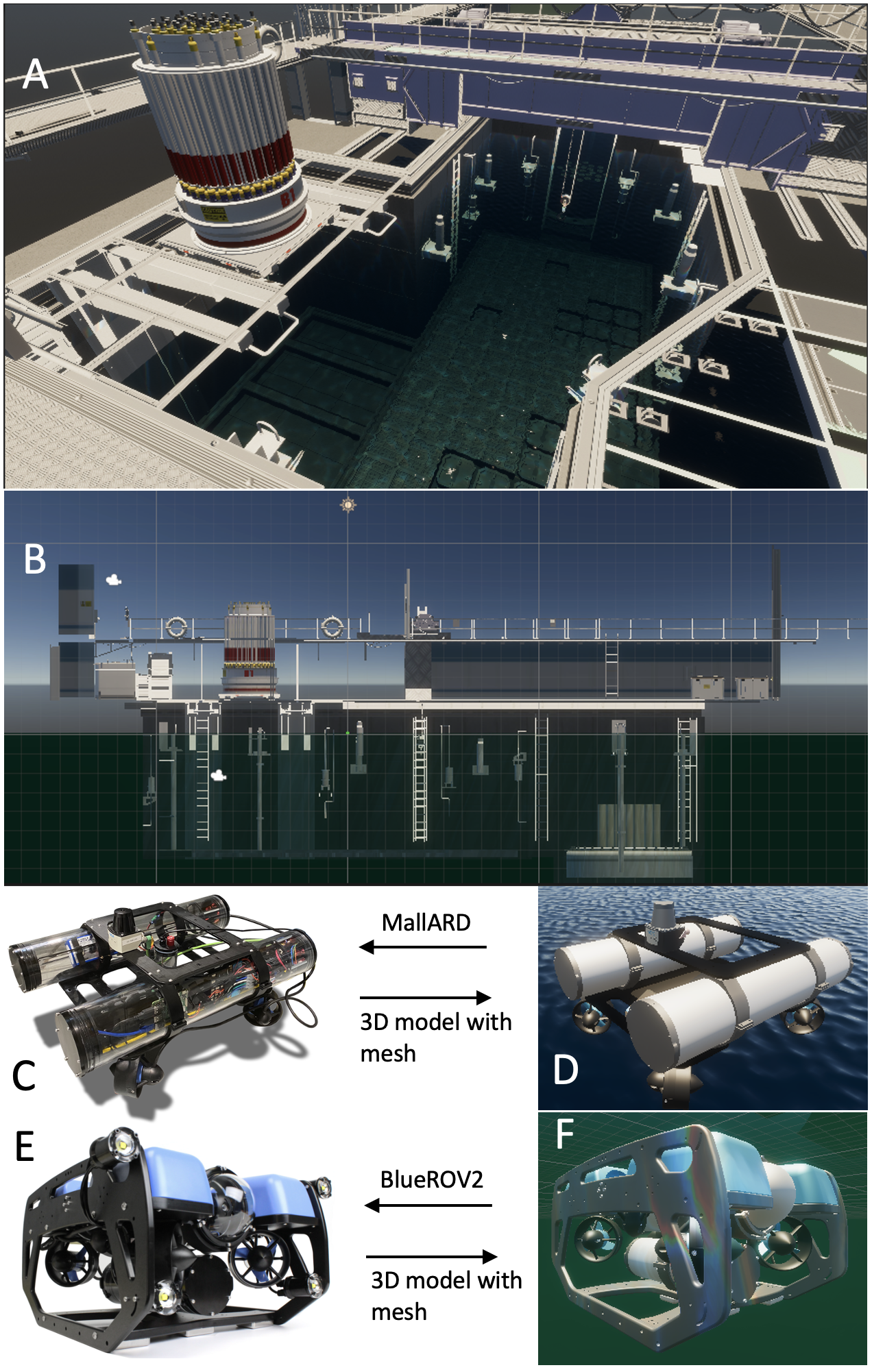
Figure 5: Simulation environment scenario and robots. (A) Overview of the simulated nuclear fuel pool . (B) Sideoview of the nuclear fuel pool (B) Autonomous surface robot - MallARD (D) MallARD’s 3D model in Unity (E) Commercial underwater robot - BlueROV2 (F) BlueROV2 3D model in Unity.

IV-C Simulation evaluation of CAP-SD

The simulation platform is a personal computer with an Intel Core i7 12700H CPU (central processing unit) running at 3.972 GHz and with 32-GB RAM (random access memory). In the experiments, the BlueROV2 moved in the tank while maintaining a fixed pitch and roll. In the following research, MallARD will be programmed to follow the BlueROV2 autonomously but the focus of the present research is to validate and quantify the accuracy of the proposed positioning system. All sensor data was collected via ROS and was recorded on the same roscore, which allows data to be shared in real-time and synchronised to a single clock.

To evaluate the performance of the CAP-SD system, five distinct datasets with varying motion patterns were collected. In these five datasets, the BlueROV2 operates along five distinct trajectories: square, lawnmower, bouncing, random, and two-floor. All datasets were recorded when MallARD was held stationary and BlueROV2 was moved underneath in the multi-beam sonar’s FOV. Data from all sensors was recorded and was post processed using CAP-SD. Pose information from the Unity transformation component was recorded as the ground truth.

IV-D Discussion

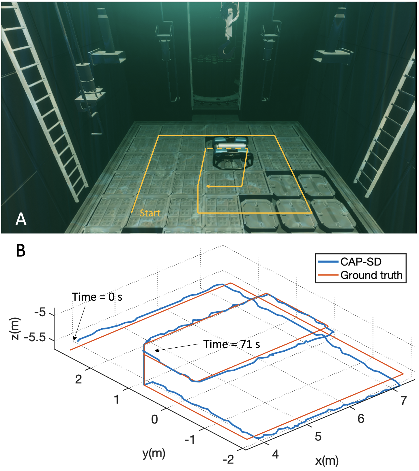
Figure 6: Plot showing the 3D trajectory of BlueROV2 estimated by CAP-SD against ground truth overtime respectively, during 71 seconds of dataset 5 (Two-floor).

Figure 6B shows the 3D trajectory of the CAP-SD alongside the ground truth. Overall, within this simulation environment, CAP-SD is capable of accurately localising the ROV. Table 5 presents the RMS error of the proposed CAP-SD methods for all five datasets. Due to the depth/pressure plugin used in this simulation not actually sensing water pressure but merely adding noise to a known absolute depth, the results do not include a comparison of the RMSE along the $z$-axis. Therefore, as detailed in Section III, the accuracy of localisation largely depends on whether the YOLOv5 model can accurately determine the bounding box (the pixel coordinates of the robot on the sonar image frame).

As indicated by the Table 5, the Euclidean RMSE remains below 200 mm for each trajectory type. In datasets 2 and 3, the values are relatively higher, approaching 200 mm. This is attributed to the BlueROV2 passing through specific locations during the bouncing and lawnmower trajectories, where, in the sonar images, the spatial overlap between the robot and other objects in the underwater environment occurs. Under these circumstances, YOLOv5 fails to provide accurate pixel coordinates for the robot, as shown in Fig 7. In Fig 7A, the robot is not significantly affected by the environment, allowing YOLOv5 to clearly detect the BlueROV2 in the sonar images. However, in certain areas, as shown in Fig 7B, this is not the case. The green bounding box indicates the expected range, while the red represents the results from YOLOv5. This is also a challenge for multi-beam sonar: signal-to-noise ratio (SNR) and resolution. Images from multi-beam sonar frequently exhibit artifacts and possess a lower resolution when contrasted with images captured by cameras [33].

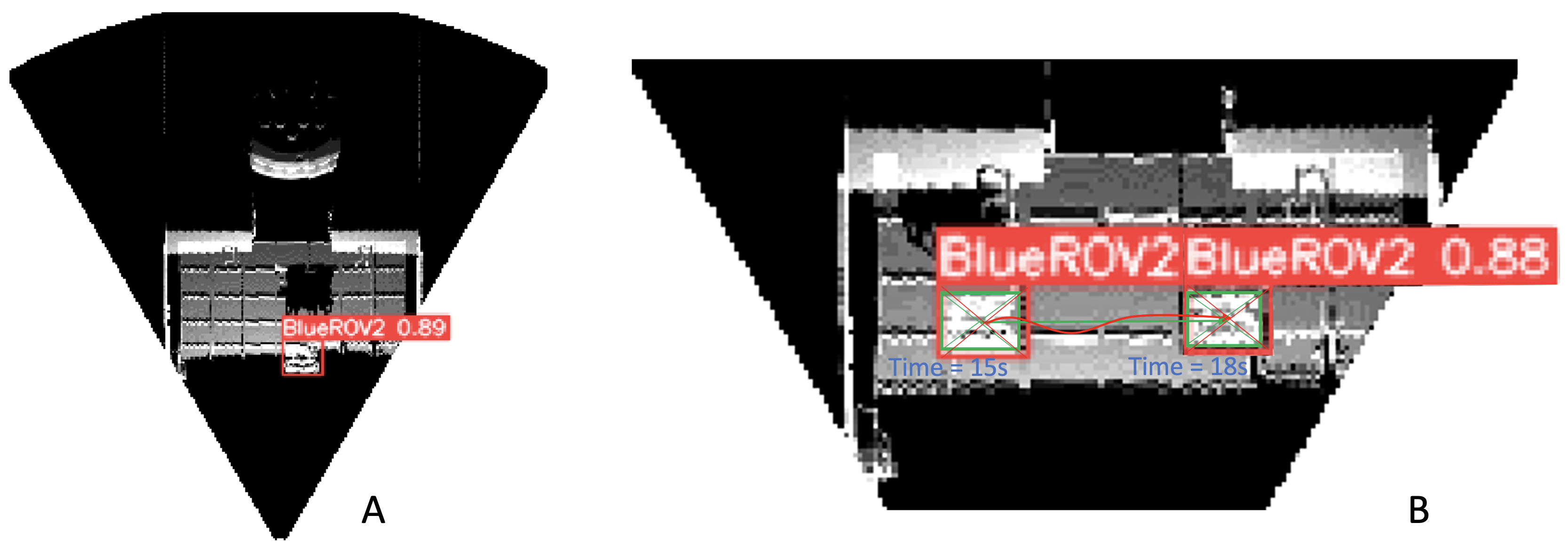
Figure 7: Sonar image view with YOLOv5 object detection. (A) Accurate robot detection by YOLOv5. (B) Due to YOLO v5’s inability to provide precise bounding boxes, errors occur in localisation. Green represents the true position, while red indicates the detection results of YOLOv5.

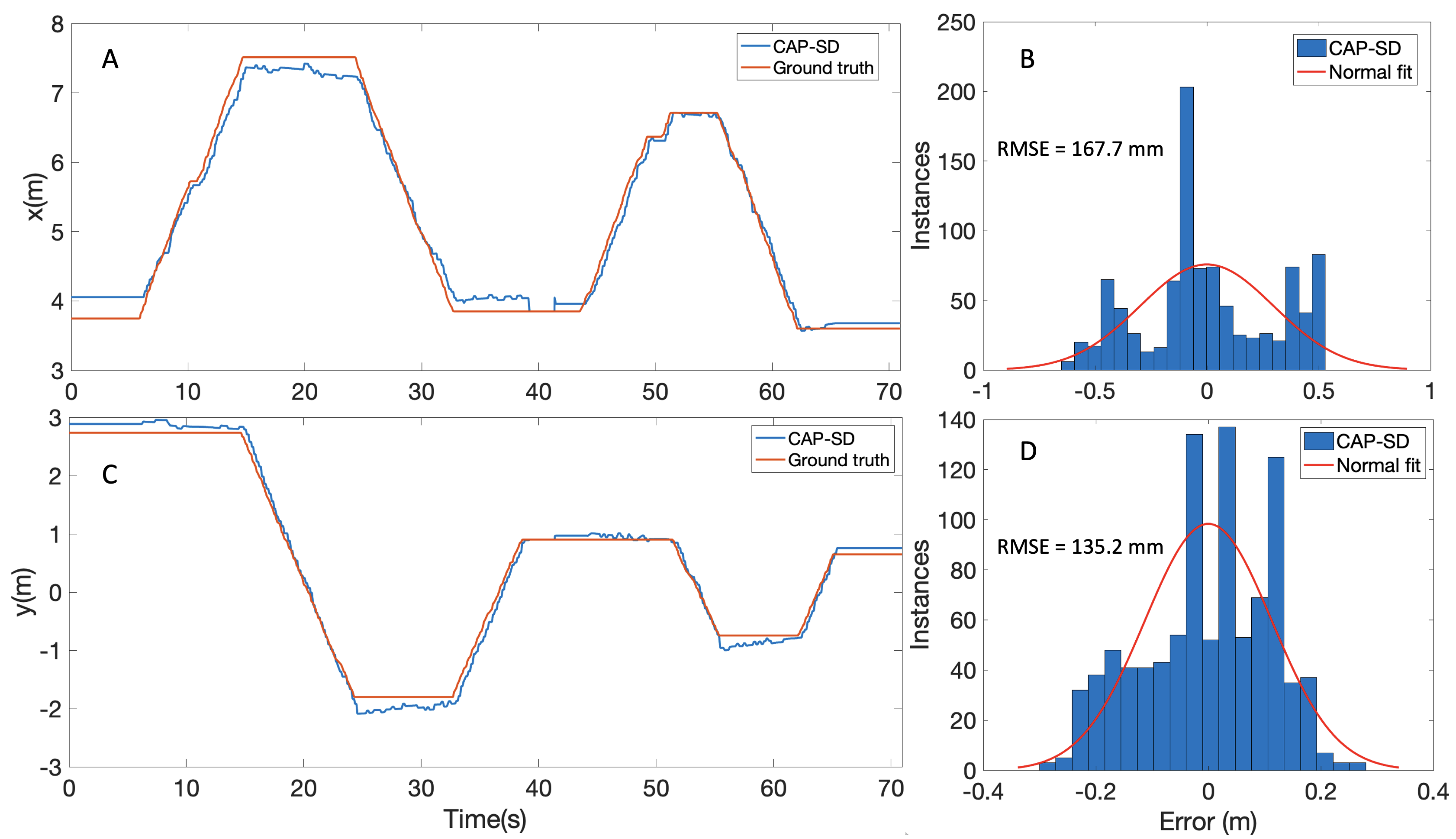
Figure 8: plots (A) and (C) shows the translation of the ROV in the the world fixed frame estimated using the two CAP-SD methods alongside the ground truth. Plots (B) and (D) show the associated error histograms for CAP-SD

TABLE I: RMS errors relative to the ground truth measurement of CAP-SD for all 5 datasets .

Dataset	Trajectory	x RMSE	y RMSE	Euclidian RMSE
1	Square	134.2 mm	129.6 mm	160.1 mm
2	Bouncing	164.7 mm	144.5 mm	201.7 mm
3	Lawnmower	162.6 mm	147.3 mm	206.5 mm
4	Random	143.9 mm	134.7 mm	180.2 mm
5	Two-floor	167.7 mm	135.2 mm	197.4 mm

V Conclusions and future works

This paper introduces a novel underwater localisation system for joint robotic operations, capable of sim-to-real applications. To the authors’ best knowledge, this is the first system applied in constrained underwater environments that does not require infrastructure, is not limited by lighting conditions, and is unaffected by water turbidity. Since it is in the proof-of-principle stage, stringent accuracy requirements have not been imposed.

This work has demonstrated the potential of the CAP system, however, there are still several challenges to overcome, including:

• MallARD’s autonomous tracking of the BlueROV based on object detection from the sonar image

• Fusing with a dead reckoning system to improve precision and account for outages in image sonar tracking

• Sensors’ synchronisation in time domain

• A deeply customized neural network designed specifically to detect objects in sonar images

• Real-world experimental evaluation

This research offers significant potential for extension in several directions:

• Joint above-water and underwater 3D reconstruction in static/dynamic aquatic environments

• Path planning for surface robots serving as external tracking systems to enhance the 3D SLAM capabilities of underwater robots

• Temporal synchronisation of sensors distributed across multiple robotic agents

References

- [1] C. Zhao, P. R. Thies, and L. Johanning, “Offshore inspection mission modelling for an ASV/ROV system,” Ocean Engineering, vol. 259, p. 111899, 2022.
- [2] A. Griffiths, A. Dikarev, P. R. Green, B. Lennox, X. Poteau, and S. Watson, “AVEXIS—aqua vehicle explorer for in-situ sensing,” IEEE Robotics and Automation Letters, vol. 1, no. 1, pp. 282–287, 2016.
- [3] D. A. Duecker, A. R. Geist, E. Kreuzer, and E. Solowjow, “Learning environmental field exploration with computationally constrained underwater robots: Gaussian processes meet stochastic optimal control,” Sensors, vol. 19, no. 9, p. 2094, 2019.
- [4] P. Ozog, N. Carlevaris-Bianco, A. Kim, and R. M. Eustice, “Long-term mapping techniques for ship hull inspection and surveillance using an autonomous underwater vehicle,” Journal of Field Robotics, vol. 33, no. 3, pp. 265–289, 2016.
- [5] X. M. Lv, Y. F. Liu, H. B. Gao, L. Ding, J. G. Tao, K. R. Xia, and Z. Q. Deng, “Design of underwater welding robot used in nuclear plant,” in Key Engineering Materials, vol. 620, pp. 484–489, Trans Tech Publ, 2014.
- [6] S. Watson, D. A. Duecker, and K. Groves, “Localisation of unmanned underwater vehicles (UUVs) in complex and confined environments: A review,” Sensors, vol. 20, no. 21, p. 6203, 2020.
- [7] U. K. Verfuss, A. S. Aniceto, D. V. Harris, D. Gillespie, S. Fielding, G. Jiménez, P. Johnston, R. R. Sinclair, A. Sivertsen, S. A. Solbø, et al., “A review of unmanned vehicles for the detection and monitoring of marine fauna,” Marine pollution bulletin, vol. 140, pp. 17–29, 2019.
- [8] T. Sakaue, T. Nagakita, T. Kaneda, Y. Yamashita, K. Nishizawa, K. Kanbara, H. Hanaoka, S. Shirai, S. Kikuchi, and D. Uchijima, “Development of USV Used in Underground Floors Surveying of the Contaminated Buildings at Fukushima Daiichi NPS,” in IEEE International Symposium on Safety, Security, and Rescue Robotics (SSRR), pp. 224–229, 2022.
- [9] R. R. Khan, T. Taher, and F. S. Hover, “Accurate geo-referencing method for auvs for oceanographic sampling,” in OCEANS 2010 MTS/IEEE SEATTLE, pp. 1–5, 2010.
- [10] M. Morgado, P. Oliveira, and C. Silvestre, “Tightly coupled ultrashort baseline and inertial navigation system for underwater vehicles: An experimental validation,” Journal of Field Robotics, vol. 30, no. 1, pp. 142–170, 2013.
- [11] Sonardyne, “Micro-ranger 2 USBL.” https://www.sonardyne.com/products/micro-ranger-2-shallow-water-usbl-system/. accessed: 2023-03-15.
- [12] S. Rahman, A. Quattrini Li, and I. Rekleitis, “Svin2: A multi-sensor fusion-based underwater slam system,” The International Journal of Robotics Research, vol. 41, no. 11-12, pp. 1022–1042, 2022.
- [13] S. Leutenegger, S. Lynen, M. Bosse, R. Siegwart, and P. Furgale, “Keyframe-based visual–inertial odometry using nonlinear optimization,” The International Journal of Robotics Research, vol. 34, no. 3, pp. 314–334, 2015.
- [14] T. Qin, P. Li, and S. Shen, “VINS-Mono: A robust and versatile monocular visual-inertial state estimator,” IEEE Transactions on Robotics, vol. 34, no. 4, pp. 1004–1020, 2018.
- [15] C. Campos, R. Elvira, J. J. G. Rodríguez, J. M. Montiel, and J. D. Tardós, “ORB-SLAM3: An accurate open-source library for visual, visual-inertial, and multimap SLAM,” IEEE Transactions on Robotics, vol. 37, no. 6, pp. 1874–1890, 2021.
- [16] D. Ribas, P. Ridao, J. Neira, and J. D. Tardos, “SLAM using an imaging sonar for partially structured underwater environments,” in IEEE/RSJ international conference on intelligent robots and systems, pp. 5040–5045, IEEE, 2006.
- [17] A. Mallios, P. Ridao, D. Ribas, M. Carreras, and R. Camilli, “Toward autonomous exploration in confined underwater environments,” Journal of Field Robotics, vol. 33, no. 7, pp. 994–1012, 2016.
- [18] D. A. Duecker, N. Bauschmann, T. Hansen, E. Kreuzer, and R. Seifried, “Towards micro robot hydrobatics: Vision-based guidance, navigation, and control for agile underwater vehicles in confined environments,” in IEEE/RSJ International Conference on Intelligent Robots and Systems, pp. 1819–1826, 2020.
- [19] Qualisys, “Miqus.” https://www.qualisys.com/cameras/miqus/, 2022. accessed: 2023-03-15.
- [20] J. Snyder, “Doppler velocity log navigation for observation-class ROVs,” Sea Technology, vol. 51, no. 12, pp. 27–30, 2010.
- [21] G. Fukuda, D. Hatta, X. Guo, and N. Kubo, “Performance evaluation of imu and dvl integration in marine navigation,” Sensors, vol. 21, no. 4, p. 1056, 2021.
- [22] L. Luo, Y. Huang, Z. Zhang, and Y. Zhang, “A New Kalman Filter-Based In-Motion Initial Alignment Method for DVL-Aided Low-Cost SINS,” IEEE Transactions on Vehicular Technology, vol. 70, no. 1, pp. 331–343, 2021.
- [23] D. Wang, X. Xu, Y. Yao, T. Zhang, and Y. Zhu, “A novel SINS/DVL tightly integrated navigation method for complex environment,” IEEE Transactions on Instrumentation and Measurement, vol. 69, no. 7, pp. 5183–5196, 2020.
- [24] R. H. Rogne, T. H. Bryne, T. I. Fossen, and T. A. Johansen, “MEMS-based inertial navigation on dynamically positioned ships: Dead reckoning,” IFAC-PapersOnLine, vol. 49, no. 23, pp. 139–146, 2016.
- [25] M. Sung, J. Kim, H. Cho, M. Lee, and S.-C. Yu, “Underwater-sonar-image-based 3d point cloud reconstruction for high data utilization and object classification using a neural network,” Electronics, vol. 9, no. 11, p. 1763, 2020.
- [26] M. D. Aykin and S. Negahdaripour, “Forward-look 2d sonar image formation and 3d reconstruction,” in 2013 OCEANS-San Diego, pp. 1–10, IEEE, 2013.
- [27] S. Kohlbrecher, J. Meyer, O. von Stryk, and U. Klingauf, “A flexible and scalable slam system with full 3d motion estimation,” in Proc. IEEE International Symposium on Safety, Security and Rescue Robotics (SSRR), IEEE, November 2011.
- [28] K. Groves, A. West, K. Gornicki, S. Watson, J. Carrasco, and B. Lennox, “MallARD: An autonomous aquatic surface vehicle for inspection and monitoring of wet nuclear storage facilities,” Robotics, vol. 8, no. 2, p. 47, 2019.
- [29] Unity Technologies, “Unity.” https://unity.com/. accessed: 2024-02-05.
- [30] I. Lončar, J. Obradović, N. Kraševac, L. Mandić, I. Kvasić, F. Ferreira, V. Slošić, Đ. Nađ, and N. Mišković, “MARUS-a marine robotics simulator,” in OCEANS 2022, Hampton Roads, pp. 1–7, IEEE, 2022.
- [31] NWH Coding, “Dynamic Water Physics 2.” https://assetstore.unity.com/packages/tools/physics/dynamic-water-physics-2-147990. accessed: 2024-02-05.
- [32] Open Robotics, “ROS.” http://wiki.ros.org/. accessed: 2023-03-15.
- [33] E. Westman and M. Kaess, “Degeneracy-aware imaging sonar simultaneous localization and mapping,” IEEE Journal of Oceanic Engineering, vol. 45, no. 4, pp. 1280–1294, 2019.