A canonical tree decomposition for order types,
and some applications

Abstract.

We introduce and study a notion of decomposition of planar point sets (or rather of their chirotopes) as trees decorated by smaller chirotopes. This decomposition is based on the concept of mutually avoiding sets (which we rephrase as modules), and adapts in some sense the modular decomposition of graphs in the world of chirotopes. The associated tree always exists and is unique up to some appropriate constraints. We also show how to compute the number of triangulations of a chirotope efficiently, starting from its tree and the (weighted) numbers of triangulations of its parts.

Keywords: Order type, chirotopes, modular decomposition, counting triangulations, mutually avoiding point sets, generating functions, rewriting systems.

1. Introduction

Any finite sequence $P=(p_{1},p_{2},\ldots,p_{n})$ of points in $\mathbb{R}^{2}$ gives rise to a number of combinatorial data such as the subset of extremal points, or the set of crossing-free matchings of $P$. Often, such structures depend on the coordinates of the points of $P$ only through a limited number of predicates, so one can replace the (geometric) point sequence by a purely combinatorial object. For instance, the convex hulls and crossing-free matchings are determined by the map sending every triple $1\leq i,j,k\leq n$ of indices to the orientation (positive, negative or flat) of the triangle $p_{i}p_{j}p_{k}$. For every $n$, there are finitely many such maps (called chirotope or order types, see below) and they have been extensively investigated, see e.g. the book of Björner et al. [BLVS⁺99].

In this paper we examine chirotopes from the point of view of the modular decomposition method, which is an important tool in algorithmic graph theory (see e.g. [HP10]). To this end, we define a notion of module in chirotopes, as a partition of the chirotope into two sets, such that no line going through two points of the same set separates points of the other set; see Figure 1. This is reminiscent of the concept of mutually avoiding sets, previously considered in the literature, though we use here a different perspective on such sets (see discussion and references at the end of Section 1.1). Using this notion of modules, we encode a chirotope by a tree whose nodes are themselves decorated by chirotopes, each point appearing in a single node, so that subtrees joined by an edge encode modules of the original point set.

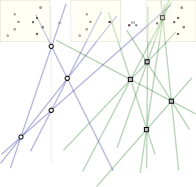
Figure 1. A set of 9 points which can be decomposed into two modules of size $4$ and $5$ points.

The main contributions presented here are the following.

• We introduce a notion of canonical chirotope tree such that each chirotope is represented by a unique canonical chirotope tree.

• We show that the proportion of realizable chirotopes that are indecomposable tends to 1.

• We show how the number of triangulations of a chirotope given by a chirotope tree can be computed from the (weighted) numbers of triangulations of its nodes.

The first and third results also hold in the more general framework of abstract chirotopes (function mapping triples of elements either to clockwise or counterclockwise, satisfying some axioms, but not necessarily corresponding to a set of points in $\mathbb{R}^{2}$; see details below). We offer in Section 1.4 several new open questions raised by this concept of chirotope tree decompositions.

Throughout the paper, all point sets are finite, planar and in general position, implying in particular that no three points are ever aligned. Adapting our construction to point sets in higher dimension would need considerable work, as our definitions really use the fact that the chirotope is a map of three arguments (in general, the chirotope of a point set in $\mathbb{R}^{d}$ takes $d+1$ arguments). On the other hand, we believe that most results could be adapted to point sets that are not necessarily in general position, but we decided not to discuss such cases for simplicity.

Given a finite set $X$, we write $(X)_{3}$ for the set of triples $(x,y,z)$ of distinct elements in $X$. We write $[n]$ for the set $\{1,2,\ldots,n\}$.

1.1. Context and motivation

Let us first provide some context on the objects, methods and questions that we consider.

Realizable chirotopes.

The chirotope of a set ${\cal P}=\{\mathcal{P}_{\ell}\}_{\ell\in X}$ of points in general position labeled by $X$ is the function

$$\chi_{\cal P}:\left\{\begin{array}[]{rcl}(X)_{3}&\to&\{-1,+1\}\\ (x,y,z)&\mapsto&\left\{\begin{array}[]{rl}+1&\text{ if $\mathcal{P}_{x},\mathcal{P}_{y},\mathcal{P}_{z}$ are in counterclockwise order,}\\ -1&\text{ if $\mathcal{P}_{x},\mathcal{P}_{y},\mathcal{P}_{z}$ are in clockwise order.}\\ \end{array}\right.\end{array}\right.$$

This function is sometimes called the labeled order type of the point set [GP83]. We say that chirotopes of point sets are realizable to distinguish them from their combinatorial (abstract) generalization.

Representing realizable chirotopes.

Deciding if a given function $(X)_{3}\to\{-1,1\}$ is a realizable chirotope turns out to be a challenging problem: it is equivalent to the existential theory of the reals [BLVS⁺99, Theorem 8.7.2] and NP-hard [Sho91]. Whether this problem is in NP is open, and, interestingly, a positive answer is equivalent to the existence of a (pseudorandom) generator that produces a realizable chirotope of size $n$ in time polynomial in $n$ while ensuring that every element has nonzero probability. The space of realizable chirotopes is therefore difficult to explore, which makes it hard to test efficiently some conjectures in discrete geometry or to check experimentally a geometric algorithm in the exact geometric computing paradigm [SY17]. The present work grew out of an attempt to devise new ways of constructing and representing (large) realizable chirotopes.

Abstract chirotopes.

As mentioned above, most of our results hold in a more general setting. Let us define a chirotope on a finite set $X$ as a function $\chi:(X)_{3}\to\{-1,1\}$ that satisfies the following properties:

(symmetry):

for any distinct $x,y,z\in X$,

(1) $$\chi(x,y,z)=\chi(y,z,x)=\chi(z,x,y)=-\chi(z,y,x)=-\chi(y,x,z)=-\chi(x,z,y);$$

(interiority):

for any distinct $t,x,y,z\in X$,

(2) $$\chi(t,y,z)=\chi(x,t,z)=\chi(x,y,t)=1\quad\Rightarrow\quad\chi(x,y,z)=1;$$

(transitivity):

for any distinct $s,t,x,y,z\in X$,

(3) $$\chi(t,s,x)=\chi(t,s,y)=\chi(t,s,z)=\chi(x,y,t)=\chi(y,z,t)=1\quad\Rightarrow\quad\chi(x,z,t)=1.$$

It can be proven that any realizable chirotope is a chirotope. We may use the term abstract chirotope to mean a chirotope that is not necessarily realizable. Lastly, for readers acquainted with matroid theory, let us note that abstract chirotopes are in correspondence with the relabeling classes of acyclic uniform oriented matroids of rank 3 [BLVS⁺99].

Notions and properties for point sets that can be expressed only through orientations of triples of points generalize to abstract chirotopes. For example, an element $x\in X$ is extreme in a chirotope $\chi$ on $X$ if there exists $y\in X\setminus\{x\}$ such that $\chi(x,y,z)$ is the same for all $z\in X\setminus\{x,y\}$. With this definition, extreme elements of realizable chirotopes correspond precisely to the vertices of their convex hulls.

Triangulations.

Counting the triangulations supported by a given set of $n$ points is a classical problem in computational geometry (see the discussion in [MM16]). The fastest known algorithm is due to Marx and Miltzow [MM16] and has complexity $\mathcal{O}(n^{(11+o(1))\sqrt{n}})$. It is quite involved, and a simpler solution, due to Alvarez and Seidel [AS13], runs in time $\mathcal{O}(n^{2}2^{n})$.

Given a point set $P=\{\mathcal{P}_{\ell}\}_{\ell\in X}$, two segments $\mathcal{P}_{x}\mathcal{P}_{y}$ and $\mathcal{P}_{z}\mathcal{P}_{t}$ with distinct endpoints in $P$ cross if and only if $\chi_{P}(x,y,z)=-\chi_{P}(x,y,t)$ and $\chi_{P}(z,t,x)=-\chi_{P}(z,t,y)$. We can therefore define the crossing of segments for abstract chirotopes. A segment in a chirotope $\chi$ on $X$ is a pair of elements of $X$, and the segments $xy$ and $zt$ cross in $\chi$ if they satisfy the above condition. A triangulation of $\chi$ is an inclusion-maximal family of segments such that no two cross in $\chi$. The algorithm of Alvarez and Seidel easily generalizes to abstract chirotopes.

Modular decomposition.

The gist of modular decomposition is to break down discrete structures to allow efficient recursion. These decompositions usually start by partitioning the elements of the structure so that any two elements in a part (also called a module) are indistinguishable “from the outside”. Choosing this partition as coarse as possible while being nontrivial, and iterating the decomposition within each part yields a decomposition tree. These ideas originated in graph theory [Gal67], where modules gather vertices with the same neighbors outside of the module, and several hereditary classes of graphs have well-behaved modular decompositions, e.g. comparability graphs, permutation graphs and cographs [HP10]. We also note that a variant of modular decomposition, called split decomposition, has been thoroughly studied in graph theory; see, e.g., [Rao08]. Interestingly, our chirotope tree decomposition share some features with both the modular and split decompositions: our notion of modules is closer to that of modules in graph than to that of split, but our decomposition tree are unrooted and unordered, as split decomposition trees.

Other examples of structures for which modular decompositions were developed include boolean functions, set systems and permutations [MR84, AA05]. Each structure requires an ad hoc analysis that the proposed notion of modules leads to a well-defined decomposition, where each object has a unique decomposition tree. The proportion of objects with nontrivial decomposition is often vanishingly small. Nevertheless, such decompositions proved useful e.g. in devising fixed-parameter polynomial algorithms for hard algorithmic problems [HP10, $\mathsection 7$] or in studying subclasses of objects [BBR11, CFL17].

Mutual avoiding point sets.

Let us discuss the link with the notion of mutually avoiding subsets, as considered in the litterature. Two planar point sets are mutually avoiding if no line through two points from one set separates two points from the other set. Any set of $n$ points in general position contains two mutually avoiding subsets of size $\Omega(\sqrt{n})$ each [AEG⁺94], a bound that is asymptotically best possible [Val97], and smaller mutually avoiding subsets are actually abundant [SZ23, Theorem 1.3]. Mutually avoiding subsets have been applied to the study of crossing families [AEG⁺94] and empty $k$-gons [Val97].

The modules we consider here are mutually avoiding subsets that cover the whole chirotope. Our work goes in a different direction than the above cited works in that they are looking for mutually avoiding subsets contained in a chirotope, whereas we look for mutually avoiding subsets that decompose a chirotope. Our analysis thus applies to a more restricted class of chirotopes, the (highly) decomposable ones, but gives more information on their structure.

1.2. Our results

We now define our decomposition and state our main results.

Bowtie decomposition.

The fact that a point set can be split into two modules $P$ and $Q$ has two interesting consequences at the level of chirotopes. First, the chirotope on point set $P\cup\{p^{*}\}$, which we denote $\chi_{P\cup\{p^{*}\}}$, is, up to relabeling, independent of the choice of the point $p^{*}\in Q$. Second, the chirotope $\chi_{P\cup Q}$ on point set $P\cup Q$ is completely determined by the chirotopes $\chi_{P\cup\{p^{*}\}}$ and $\chi_{Q\cup\{q^{*}\}}$ for any choices of $p^{*}\in Q$ and $q^{*}\in P$. We can use this to decompose $\chi_{P\cup Q}$ in terms of $\chi_{P\cup\{p^{*}\}}$ and $\chi_{Q\cup\{q^{*}\}}$.

Let us express this decomposition. Throughout the paper, we call sign function on a set $X$, a function $(X)_{3}\to\{-1,+1\}$ that is only required to satisfy the symmetry condition (1). Let $X$ and $Y$ be disjoint sets, and let $x^{*}\notin X$ and $y^{*}\notin Y$. Given two sign functions $\chi$ on $X\cup\{x^{*}\}$ and $\xi$ on $Y\cup\{y^{*}\}$, we define the bowtie $\kappa\stackrel{{\scriptstyle\text{def}}}{{=}}\chi\mathchoice{\sideset{{}_{x^{*}}}{{}_{y^{*}}}{\operatorname{\textup{\Bowtie}}}}{\sideset{{}_{x^{*}}}{{}_{y^{*}}}{\operatorname{\textup{\Bowtie}}}}{\sideset{{}_{x^{*}}}{{}_{y^{*}}}{\scriptstyle\operatorname{\textup{\Bowtie}}}}{\sideset{{}_{x^{*}}}{{}_{y^{*}}}{\scriptstyle\operatorname{\textup{\Bowtie}}}}\xi$ as the sign function on $X\cup Y$ satisfying:

(4) $$\left\{\begin{array}[]{rcll}\kappa(x_{1},x_{2},x_{3})&=&\chi(x_{1},x_{2},x_{3})&\text{ if $x_{1},x_{2},x_{3}$ are all in $X$;}\\ \kappa(x_{1},x_{2},y)&=&\chi(x_{1},x_{2},x^{*})&\text{ if $x_{1},x_{2}$ are in $X$ and $y$ is in $Y$;}\\ \kappa(x,y_{2},y_{3})&=&\xi(y^{*},y_{2},y_{3})&\text{ if $x$ is in $X$ and $y_{2},y_{3}$ are in $Y$;}\\ \kappa(y_{1},y_{2},y_{3})&=&\xi(y_{1},y_{2},y_{3})&\text{ if $y_{1},y_{2},y_{3}$ are all in $Y$.}\end{array}\right.$$

With the symmetry condition (1), this completely defines $\kappa$ on $(X\cup Y)_{3}$. Informally, this amounts to computing the sign function as in $\chi$ (resp. $\xi$) if the majority of the elements come from $X$ (resp. $Y$), possibly replacing the only element outside $X$ (resp. $Y$) by $x^{*}$ (resp. $y^{*}$).

Note that for disjoint modules $P$ and $Q$ of $P\cup Q$, we have $\chi_{P\cup Q}=\chi_{P\cup\{p^{*}\}}\mathchoice{\sideset{{}_{p^{*}}}{{}_{q^{*}}}{\operatorname{\textup{\Bowtie}}}}{\sideset{{}_{p^{*}}}{{}_{q^{*}}}{\operatorname{\textup{\Bowtie}}}}{\sideset{{}_{p^{*}}}{{}_{q^{*}}}{\scriptstyle\operatorname{\textup{\Bowtie}}}}{\sideset{{}_{p^{*}}}{{}_{q^{*}}}{\scriptstyle\operatorname{\textup{\Bowtie}}}}\chi_{Q\cup\{q^{*}\}}$ for any choice of $p^{*}\in Q$ and $q^{*}\in P$.

Bowtie products.

While defined on sign functions, the bowtie operator also allows to combine smaller chirotopes into larger ones. This works under the following conditions.

Proposition 1.1.

Let $X$ and $Y$ be disjoint sets, with $|X|,|Y|\geq 2$, and let $x^{*}\notin X$ and $y^{*}\notin Y$. Let $\chi$ and $\xi$ be chirotopes on $X\cup\{x^{*}\}$ and $Y\cup\{y^{*}\}$.

1. $\chi\mathchoice{\sideset{{}_{x^{*}}}{{}_{y^{*}}}{\operatorname{\textup{\Bowtie}}}}{\sideset{{}_{x^{*}}}{{}_{y^{*}}}{\operatorname{\textup{\Bowtie}}}}{\sideset{{}_{x^{*}}}{{}_{y^{*}}}{\scriptstyle\operatorname{\textup{\Bowtie}}}}{\sideset{{}_{x^{*}}}{{}_{y^{*}}}{\scriptstyle\operatorname{\textup{\Bowtie}}}}\xi$ is a chirotope if and only if $x^{*}$ and $y^{*}$ are extreme in $\chi$ and $\xi$.

2. $\chi\mathchoice{\sideset{{}_{x^{*}}}{{}_{y^{*}}}{\operatorname{\textup{\Bowtie}}}}{\sideset{{}_{x^{*}}}{{}_{y^{*}}}{\operatorname{\textup{\Bowtie}}}}{\sideset{{}_{x^{*}}}{{}_{y^{*}}}{\scriptstyle\operatorname{\textup{\Bowtie}}}}{\sideset{{}_{x^{*}}}{{}_{y^{*}}}{\scriptstyle\operatorname{\textup{\Bowtie}}}}\xi$ is a realizable chirotope if and only if $\chi$ and $\xi$ are realizable and $x^{*}$ and $y^{*}$ are extreme in $\chi$ and $\xi$.

3. If $\chi\mathchoice{\sideset{{}_{x^{*}}}{{}_{y^{*}}}{\operatorname{\textup{\Bowtie}}}}{\sideset{{}_{x^{*}}}{{}_{y^{*}}}{\operatorname{\textup{\Bowtie}}}}{\sideset{{}_{x^{*}}}{{}_{y^{*}}}{\scriptstyle\operatorname{\textup{\Bowtie}}}}{\sideset{{}_{x^{*}}}{{}_{y^{*}}}{\scriptstyle\operatorname{\textup{\Bowtie}}}}\xi$ is a chirotope, then the extreme elements of $\chi\mathchoice{\sideset{{}_{x^{*}}}{{}_{y^{*}}}{\operatorname{\textup{\Bowtie}}}}{\sideset{{}_{x^{*}}}{{}_{y^{*}}}{\operatorname{\textup{\Bowtie}}}}{\sideset{{}_{x^{*}}}{{}_{y^{*}}}{\scriptstyle\operatorname{\textup{\Bowtie}}}}{\sideset{{}_{x^{*}}}{{}_{y^{*}}}{\scriptstyle\operatorname{\textup{\Bowtie}}}}\xi$ are the elements of $X\cup Y$ extreme in $\chi$ or in $\xi$.

The above proposition is proved in Section 3.1. We also show (Proposition 3.11) that $\Bowtie$ has associativity and commutativity properties. We say that a chirotope $\kappa$ is decomposable if there exist chirotopes $\chi$ and $\xi$, each on a strictly smaller set, such that $\kappa=\chi\mathchoice{\sideset{{}_{x^{*}}}{{}_{y^{*}}}{\operatorname{\textup{\Bowtie}}}}{\sideset{{}_{x^{*}}}{{}_{y^{*}}}{\operatorname{\textup{\Bowtie}}}}{\sideset{{}_{x^{*}}}{{}_{y^{*}}}{\scriptstyle\operatorname{\textup{\Bowtie}}}}{\sideset{{}_{x^{*}}}{{}_{y^{*}}}{\scriptstyle\operatorname{\textup{\Bowtie}}}}\xi$. If no such $\chi$ and $\xi$ exist we say that $\kappa$ is indecomposable.

Chirotope trees.

Formally, a chirotope tree is a tree whose nodes are decorated with chirotopes on disjoint ground sets of size at least $3$, and whose edges select an element in the ground set of each of their extremities so that (i) no element is selected more than once, and (ii) each selected element is extreme in its chirotope. Any element selected by an edge of the chirotope tree is called a proxy; for illustration purposes, we write the decorating chirotope as the label of the node (if it is realizable, we may draw a realization) and we draw edges of the tree and proxy elements in red, with the edge connecting the proxy elements. Here are two examples.

Chirotope of a chirotope tree.

To any chirotope tree $T=(V_{T},E_{T})$ we associate a sign function $\chi_{T}$ as follows. For a node $v$ of $T$, let $\chi_{v}$ denote the chirotope decorating it, and let $X_{v}$ denote the set of non-proxy elements of the ground set of $\chi_{v}$. For $x\in\cup_{w\in V_{T}}X_{w}$, the representative $R_{T}(x,v)$ of $x$ in the node $v$ is $x$ if $x\in X_{v}$, and otherwise it is the label of the proxy selected in $\chi_{v}$ by the first edge on the path in $T$ from $v$ to the node containing $x$. For distinct $x,y,z\in\cup_{w\in V_{T}}X_{w}$, we let $v(x,y,z)$ be the intersection node of the paths in $T$ from $x$ to $y$, from $y$ to $z$ and from $x$ to $z$ (if two or three elements among $x$, $y$, $z$ are in the same $X_{w}$, then we set $v(x,y,z)=w$). We define a sign function $\chi_{T}$ on $\cup_{w\in V_{T}}X_{w}$ by

(5) $$\chi_{T}(x,y,z)\stackrel{{\scriptstyle\text{def}}}{{=}}\chi_{v}(R(x,v),R(y,v),R(z,v))\qquad\text{for }v=v(x,y,z).$$

For example, if $T$ is the chirotope tree on the right in the previous picture we have $\chi_{T}(a,c,f)=\kappa(r^{*},s^{*},t^{*})=-1$, where $\kappa$ is the chirotope decorating the central node. The definition of $\chi_{T}$ ensures the following property: if removing an edge in a tree $T$ produces two subtrees $T_{1}$ and $T_{2}$, then $\chi_{T}$ is the bowtie product of $\chi_{T_{1}}$ and $\chi_{T_{2}}$ (see Lemma 4.1). Furthermore, this notion behaves well with those of chirotopes and of realizability.

Proposition 1.2.

For any chirotope tree $T$, $\chi_{T}$ is a chirotope. Moreover, if all chirotopes decorating a node in $T$ are realizable, then $\chi_{T}$ is realizable.

By Proposition 1.1(iii), the extreme elements of $\chi_{T}$ are the non-proxy extreme elements of its decorating chirotopes. Hence, if $T$ has $k$ nodes, then $\chi_{T}$ has at least $k+2$ extreme elements. Indeed, as each node has at least $3$ extreme elements and $T$ has exactly $k-1$ edges, therefore $2(k-1)$ proxies, there are at least $3k-2(k-1)=k+2$ extreme elements in $\chi_{T}$.

Canonical chirotope trees.

Let us consider a chirotope tree $T$ and a node $v$ of $T$. If $\chi_{v}=\kappa\mathchoice{\sideset{{}_{s^{*}}}{{}_{t^{*}}}{\operatorname{\textup{\Bowtie}}}}{\sideset{{}_{s^{*}}}{{}_{t^{*}}}{\operatorname{\textup{\Bowtie}}}}{\sideset{{}_{s^{*}}}{{}_{t^{*}}}{\scriptstyle\operatorname{\textup{\Bowtie}}}}{\sideset{{}_{s^{*}}}{{}_{t^{*}}}{\scriptstyle\operatorname{\textup{\Bowtie}}}}\xi$ is decomposable, then $v$ can be replaced by two nodes decorated with $\kappa$ and $\xi$, connected by an edge, so that the resulting chirotope tree $T^{\prime}$ satisfies $\chi_{T^{\prime}}=\chi_{T}$ (see Section 4.2 for details). Hence, a chirotope $\chi$ corresponds to many chirotope trees, at least one of which is decorated only by indecomposable chirotopes. However, even requesting the chirotopes decorating the nodes to be indecomposable does not ensure that a unique chirotope tree represents a given chirotope. Here are two trees with only indecomposable decorations and the same associated chirotope on $\{a,b,c,d,e,f,g\}$.

It turns out that the convex chirotopes (a chirotope is convex if all its elements are extreme) are the only source of redundancy; in the above example, the chirotope is not convex, but its restriction to $\{a,b,c,d,e\}$ is. This leads us to define a chirotope tree as canonical if every node is decorated by a convex or indecomposable chirotope, and if no edge connects two nodes decorated by convex chirotopes.

Theorem 1.3.

For any chirotope $\chi$, there is a unique canonical chirotope tree $T$ with $\chi_{T}=\chi$.

We prove this theorem in Section 4.3.

Counting triangulations.

Let $\mathcal{T}_{\kappa}$ denote the set of triangulations of a chirotope $\kappa$ on $X$. Given $x^{*}\in X$, we let $P_{\kappa,x^{*}}(s)=\sum_{T\in\mathcal{T}_{\kappa}}s^{\deg_{T}(x^{*})}$ denote the generating polynomial of the triangulations of $\kappa$, marking the degree of $x^{*}$. We prove that if $\kappa=\chi\mathchoice{\sideset{{}_{x^{*}}}{{}_{y^{*}}}{\operatorname{\textup{\Bowtie}}}}{\sideset{{}_{x^{*}}}{{}_{y^{*}}}{\operatorname{\textup{\Bowtie}}}}{\sideset{{}_{x^{*}}}{{}_{y^{*}}}{\scriptstyle\operatorname{\textup{\Bowtie}}}}{\sideset{{}_{x^{*}}}{{}_{y^{*}}}{\scriptstyle\operatorname{\textup{\Bowtie}}}}\xi$, then

(6) $$|{\cal T}_{\kappa}|=\sum_{\begin{subarray}{c}T^{\prime}\in\mathcal{T}_{\chi}\\ T^{\prime\prime}\in\mathcal{T}_{\xi}\end{subarray}}\binom{\deg_{T^{\prime}}(x^{*})+\deg_{T^{\prime\prime}}(y^{*})-2}{\deg_{T^{\prime}}(x^{*})-1}=\sum_{a,b\geq 2}\tbinom{a+b-2}{a-1}[s^{a}]P_{\chi,x^{*}}(s)\ [t^{b}]P_{\xi,y^{*}}(t).$$

More generally, given a chirotope tree $T$, we can compute the number of triangulations of $\chi_{T}$ given, for each node $v$, the generating polynomial $P_{v}$ of the triangulations of its decorating chirotope $\chi_{v}$ that marks not only the degrees of each proxy, but also the presence of each pair of proxies as an edge in the triangulation. This can be used on the one hand to find explicit formulas for the number of triangulations of some families of point sets, and on the other hand to design an effective algorithm to compute the number of triangulations of a chirotope, given its decomposition tree.

In Section 8.3, we consider a family $\mathcal{F}$ of chirotope trees, whose underlying trees are chains (a.k.a. paths), with all nodes decorated with the same chirotope. For such chirotopes, we obtain some recurrence formula for the generating polynomials of triangulations with some catalytic parameters. These recurrences are solved via the kernel method from analytic combinatorics, leading to a closed formula for the number of triangulations of any chirotope whose tree is in $\mathcal{F}$ (Proposition 8.3).

For the algorithmic aspect, we recall that, if $\chi_{v}$ has $n_{v}$ points, $k$ of which are proxies, then $P_{v}$ has $k+\binom{k}{2}$ variables, and it can be computed from $\chi_{v}$ in time $O\left(2^{n_{v}+4k}n_{v}^{k+2}\right)$ by a simple modification of the Alvarez-Seidel algorithm [AS13]. The following result gives a precise bound on the complexity of counting triangulations, given the polynomials $P_{v}$.

Proposition 1.4.

Let $T$ be a chirotope tree with $m$ edges, in which each node has degree at most $k$, and such that $\chi_{T}$ has size $n$. The number of triangulations of $\chi_{T}$ can be computed from the polynomials $\{P_{v}\colon v\text{ a node of }T\}$ in time $O\left(2^{4k}n^{2k}m\right)$ in the Real-RAM model.

We implemented our method for trees of arity $3$ (see Section 9.3 for the details and access to the code). This implementation is merely a proof of concept, and it is beyond the scope of this paper to optimize it or benchmark it, but we can mention that on a laptop, it took a few seconds to count the triangulations of the example of Figure 12 page 12, that assembles a set of $254$ points from decorating chirotopes of size $9$, and that it handles random ternary chirotope trees with 146 nodes (1024 points) in less than 5 minutes.

Proportion of decomposable chirotopes among realizable ones.

Finally, let $t_{n}$ denote the number of realizable chirotopes of size $n$ and $d_{n}$ denote the number of those that are decomposable. Our last result gives a precise estimates of $d_{n}$, in terms of $t_{n}$ and $t_{n-1}$. In particular, as announced earlier, almost all realizable chirotopes are indecomposable (as for graphs with respect to the split or modular decompositions).

Theorem 1.5.

For large $n$, we have $3\left(n-\mathcal{O}(n^{-2})\right)t_{n-1}\leq d_{n}\leq\mathcal{O}(n^{-3})t_{n}$.

Since $t_{n}$ is of order $n^{4n}$, we expect $t_{n-1}/t_{n}$ to behave as $\Theta(n^{-4})$ (but only an upper bound of this order is known). If this is indeed the case, the lower bound in our theorem behaves as $\Theta(n^{-3})t_{n}$, i.e. our bounds are tight up to multiplicative constants. Note that we do not have an analogue result for abstract chirotopes.

1.3. Discussion and related work

Originality with respect to other modular decomposition theories.

The theory of modular decomposition [MR84] does not offer any unifying model that specializes to various structures, but rather proposes general guidelines for developing such a theory. The implementation of these guidelines usually requires analyses that are specific to the objects at hand, and the case of chirotopes is no exception: almost every step requires some specific geometric idea(s).

Among realizable chirotopes, the proportion of indecomposable ones tends to $\mathbf{1}$.

This is analogue to the well-known fact that most graphs are prime graphs for the modular decomposition. The proof is, however, much more difficult and interesting than in the graph case because (i) the number of realizable chirotopes grows slower than the number of graphs on $n$ vertices and (ii) this number is only known up to exponential corrections. In particular, our proof uses some geometric constructions and is specific to the realizable setting.

Let us also mention that even if most graphs are prime graphs for the modular decomposition, this decomposition has turned out useful in many ways: design of efficient algorithms [HP10], enumeration and study of specific classes [BBF⁺22], … Similarly, for chirotopes, our tree decomposition allows one for example to construct families of large chirotopes for which enumerating triangulations is algorithmically easy (see Section 7).

Recursive constructions of point sets.

Recursive constructions of point sets abund in discrete geometry, and with some care several of them directly translate into recursively defined canonical chirotope trees (e.g. Horton sets). We are not aware of systematic decomposition methods for point sets similar to chirotope trees. The closest predecessor to (and inspiration for) this work is the recursive decomposition of chains used by Rutschmann and Wettstein [RW23, Theorem 15] to produce a new lower bound on the maximal number of triangulations of a set of $n$ points in the plane. Their representation applies to a smaller subset of order types (the chains, of which there are only exponentially many of size $n$), and decomposes every chain into parts of constant size. It allows to count the triangulations of a chain of size $n$ in $\mathcal{O}(n^{2})$ time based on ideas similar to the proof of Equation (6), but tailored to the setting of chains.

Counting triangulations.

It is interesting to compare our method for counting triangulations to the experimental results for general point sets of Alvarez and Seidel [AS13], and for chains by Rutschmann and Wettstein [RW23]. An extensive comparison is beyond the scope of this paper, all the more that the methods apply to different classes of point sets and operate on different types of input. We nevertheless note the following points.

• The general method of Alvarez and Seidel takes as input an arbitrary point set. They tested three methods on high-memory hardware for various types of point sets, and none could handle any example of size $35$ or more in less than 10 minutes.

• Our method takes as input a (chirotope presented by a) chirotope tree. We tested it on randomly-generated trees with decorating chirotopes of size $9$ summing up to sets of $\sim 1000$ points; it took less than 5 minutes on a laptop to count the triangulations.

• The method of Rutschmann and Wettstein is based on formulas specific to the class of chains and could handle examples of size $2^{21}$.

To us, this is an evidence that our approach is relevant for point sets that are highly decomposable. This is similar to some of the usual benefits of modular decomposition: some hard problems enjoy simple and effective solutions for instances that decompose well.

1.4. Perspectives

Let us conclude this introduction by sampling some of directions of enquiry that this work opens.

1. Here we used canonical chirotope trees as a tool to put together large chirotopes out of smaller ones, and we therefore considered the chirotope tree as given. One could, however, start with some point set and set out to compute the decomposition tree. This raises the following computational questions. How efficiently can one find a partition of a given (realizable) chirotope into two mutually avoiding parts or decide that none exists? Or, going even further, how efficiently can one compute the canonical chirotope tree of a given (realizable) chirotope?

2. Can crossing-free structures besides triangulations be counted efficiently from the chirotope tree? What about other statistics of a chirotope such as the number of $k$-sets or the number of crossing pairs?

3. What is the proportion of indecomposable (abstract) chirotopes? (Our proof of Theorem 1.5 uses that $t_{n}/t_{n-1}\geq\Omega(n^{4})$ and we are not aware of an analogue of this in the abstract setting.)

1.5. Outline of the paper

The paper is organized as follows.

• Sections 2 and 3 introduce the notion of modules and bowties, and in particular proves Proposition 1.1.

• Section 4 introduces chirotope trees and canonical chirotope trees, and in particular proves Proposition 1.2 and Theorem 1.3.

• Sections 5 and 6 estimate the number of decomposable chirotopes, and in particular prove Theorem 1.5.

• Sections 7, 8 and 9 show how to count the triangulations of a chirotope presented by a chirotope tree, and in particular prove Proposition 1.4.

Acknowledgments

The authors thank Emo Welzl for discussion leading to footnote 1 and anonymous referees for helpful comments. This work was done while FK was a postdoctoral fellow in LORIA, funded by ANR ASPAG (ANR-17-CE40-0017), IUF and INRIA.

2. Preliminary: some properties of extreme points

Recall that an element $x\in X$ is extreme in a chirotope $\chi$ on $X$ if there exists $y\in X\setminus\{x\}$ such that $\chi(x,y,z)$ is the same for all $z\in X\setminus\{x,y\}$. We start with a standard extension to abstract chirotopes of Carathéodory’s theorem: any point not extreme in a set $X$ is contained in a triangle with vertices in $X$ (see [BLVS⁺99, Theorem 9.2.1(1)]).

Lemma 2.1.

Let $\chi$ be a chirotope on $X$. An element $t\in X$ is not extreme in $\chi$ if and only if there exist $a,b,c\in X\setminus\{t\}$ such that $\chi(t,a,b)=\chi(t,b,c)=\chi(t,c,a)=1$.

Proof.

Assume that there exist $a,b,c\in X\setminus\{t\}$ such that $\chi(t,a,b)=\chi(t,b,c)=\chi(t,c,a)=1$. For the sake of contradiction, assume in addition that $t$ is extreme in $\chi$. By definition, this means that there exists $s\in X$ such that for all $x\in X\setminus\{t,s\}$, $\chi(t,s,x)=1$. We cannot have $s=a$ as $\chi(t,a,c)=-1$. Similarly, $s\notin\{b,c\}$. Then, the tuple $\{s,t,a,b,c\}$ contradicts the transitivity axiom.

Conversely, assume that $t$ is not extreme in $\chi$. Let us choose $a_{0},a_{1}\in X$ such that $\chi(t,a_{1},a_{0})=1$. Since $t$ is not extreme, there exists $a_{2}\in X\setminus\{t,a_{0},a_{1}\}$ such that $\chi(t,a_{1},a_{2})=-1$. If $\chi(t,a_{2},a_{0})=-1$ then $a=a_{0}$, $b=a_{2}$, $c=a_{1}$ are as desired. So assume otherwise. Since $t$ is not extreme, there exists $a_{3}\in X\setminus\{t,a_{2}\}$ such that $\chi(t,a_{2},a_{3})=-1$; note that $a_{3}\notin\{t,a_{0},a_{1},a_{2}\}$. If one of $\chi(t,a_{3},a_{0})$ or $\chi(t,a_{3},a_{1})$ equals $-1$ then we have our triple ($a\in\{a_{0},a_{1}\},b=a_{3}$ and $c=a_{2}$). So assume otherwise and using that $t$ is not extreme, pick some $a_{4}\in X\setminus\{t,a_{3}\}$ such that $\chi(t,a_{3},a_{4})=-1$. Due to the previous consideration, $a_{4}$ must be different from $a_{0},a_{1}$ and $a_{2}$. And so on and so forth: since $X$ is finite we eventually find a triple as in the lemma. See Fig. 2 for an illustration. ∎

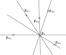
Figure 2. Illustration of the proof of Lemma 2.1 for a realizable chirotope. The points $\mathfrak{p}_{a_{i}}$ corresponding to the elements $a_{i}$ are seen from $\mathfrak{p}_{t}$ in clockwise order (since $\chi(t,a_{i},a_{i+1})=-1$ for all $i$ by construction). Given $\mathfrak{p}_{a_{i}}$, either the line $\mathfrak{p}_{a_{i}}\mathfrak{p}_{t}$ splits the point set $\{\mathfrak{p}_{a_{j}},j<i\}$ in two non trivial parts (which happens here for $i=4$), and we can find a triangle containing $\mathfrak{p}_{t}$ (namely $\mathfrak{p}_{a_{0}}\mathfrak{p}_{a_{3}}\mathfrak{p}_{a_{4}}$ in the picture), or all points $\{\mathfrak{p}_{a_{j}},j<i\}$ are on the same side of $\mathfrak{p}_{a_{i}}\mathfrak{p}_{t}$ (which happens for $i=2$ and $i=3$ here), and we let $\mathfrak{p}_{a_{i+1}}$ be any point on the other side (there is necessarily one, since $\mathfrak{p}_{t}$ is not extreme). Since the set is finite, we cannot be always in the latter situation and we eventually find a triangle containing $\mathfrak{p}_{t}$.

We now observe, for later use, that an extreme element in a chirotope defines a total order on the other elements.

Lemma 2.2.

Let $\chi$ be a chirotope on $X$, let $ext(\chi)$ be the set of extreme elements of $\chi$, and take $a\in ext(\chi)$. The relation $p<_{a}q\Leftrightarrow\chi(a,p,q)=1$ defines a strict total order on $X\setminus\{a\}$. Moreover, letting $e_{1},\ldots,e_{r}$ denotes the elements of $ext(\chi)\setminus\{a\}$ as ordered by $<_{a}$, the cyclic order $(a,e_{1},\ldots,e_{r},a)$ does not depend on the choice of $a\in ext(\chi)$.

Proof.

To prove the first assertion, we only need to check the transitivity of the relation $<_{a}$. Let us consider three elements $x,y,z\in X\setminus\{a\}$ such that $x<_{a}y$ and $y<_{a}z$, and suppose by contradiction that $z<_{a}x$. Then we have $\chi(a,x,y)=\chi(a,y,z)=\chi(a,z,x)=1$ contradicting that $a$ is extreme, by Lemma 2.1.

Let $C_{a}$ denote the cyclic order $(a,e_{1},\ldots,e_{r},a)$. To prove the second assertion, it suffices to prove that $C_{e_{1}}=C_{a}$. For every $i\in\{2,\ldots,r\}$, $e_{1}<_{a}e_{i}$. Therefore $\chi(e_{1},e_{i},a)=\chi(a,e_{1},e_{i})=1$. Hence $a$ is the maximal element for $<_{e_{1}}$. Furthermore, let $2\leq i<j\leq r$. As $e_{1}<_{a}e_{i}<_{a}e_{j}$, we have $\chi(e_{i},e_{j},a)=\chi(e_{i},a,e_{1})=1$. Then as $e_{i}$ is extreme, $\chi(e_{i},e_{1},e_{j})=-1$ by Lemma 2.1. Hence $e_{i}<_{e_{1}}e_{j}$ and $C_{e_{1}}=(e_{1},\ldots,e_{r},a,e_{1})=C_{a}$. ∎

Lemma 2.2 defines a unique cyclic order on the extreme elements of a chirotope. Geometrically, this corresponds to the anticlockwise order on the convex hull. For any extreme element $a$, it is hence possible to define its previous and next extreme element for this cyclic order, denoted respectively $a_{-}$ and $a_{+}$. Note that $a_{+}$ (resp. $a_{-}$) is the minimum (resp. maximum) element of the total order $<_{a}$.

Observation 2.3.

Recall that, by definition, an element $a$ is extreme in a chirotope $\chi$ on $X$ if and only if there exists $y$ such that $\chi(a,y,z)=1$ for all $z$ in $X\setminus\{a,y\}$. With the notation introduced above, this element $y$ is $a_{+}$: in particular it is unique. We also have the following: $a$ in extreme in $\chi$ if and only if there exists $y^{\prime}$ such that $\chi(a,y^{\prime},z)=-1$ for all $z$ in $X\setminus\{a,y\}$. When it exists, this element is also unique and corresponds to $a_{-}$ with the notation introduced above.

The last lemma of this section is of a more geometric nature, and only applies to realizable chirotopes. Given a set $\cal L$ of lines in $\mathbb{R}^{2}$, a cell of the arrangement of $\cal L$ is a connected component of $\mathbb{R}^{2}\setminus\bigcup_{\ell\in{\cal L}}\ell$.

Lemma 2.4.

Let $\chi:(X)_{3}\to\{\pm 1\}$ be a realizable chirotope and let $x\in X$ be extreme in $\chi$. Then there exists a realization $\mathcal{P}=\{\mathfrak{p}_{x},x\in X\}$ of $\chi$ such that $\mathfrak{p}_{x}$ is in an unbounded cell of the arrangement of the set of lines $\big{\{}(\mathfrak{p}_{y}\mathfrak{p}_{z})\colon y,z\in X\setminus\{x\},y\neq z\big{\}}$.

Note that this is not true for any realization of $\chi$ but only for some well-chosen realization of $\chi$: see Fig. 3 for an example of two realizations of the same chirotope, one being as in the lemma, but not the other.

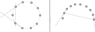
Figure 3. On the left, 10 points uniformly distributed on a circle; on the right, the same number of points uniformly distributed on a semicircle. Both configurations have the same chirotope. In the circle case, each point is in a bounded cell of the line arrangement defined by the other points (as illustrated for the left-most point). On the other hand in the semi-circle case, the left-most point is in an unbounded region of the line arrangement defined by the other points.

Proof.

This proof relies on the notion of projective transform, which we now recall; see e.g. the book of Samuel [Sam88] or Richter-Gebert [RG11] for a primer on projective geometry. For a point $\mathfrak{p}\in\mathbb{R}^{2}$ let $\hat{\mathfrak{p}}$ be the column vector $\hat{\mathfrak{p}}\stackrel{{\scriptstyle\text{def}}}{{=}}(p_{x},p_{y},1)^{t}$, and conversely, given $u\in\mathbb{R}^{3}$ with $u_{z}\neq 0$ let $\bar{u}\stackrel{{\scriptstyle\text{def}}}{{=}}(u_{x}/u_{z},u_{y}/u_{z})$. A projective transform is a map $f:\mathfrak{p}\mapsto\overline{A\hat{\mathfrak{p}}}$ with $A\in\mathbb{R}^{3\times 3}$ a non-singular matrix. Such a transform is undefined on a line of $\mathbb{R}^{2}$ (those points $\mathfrak{p}$ such that $\left(A\hat{\mathfrak{p}}\right)_{z}=0$); this line is said to be “sent to infinity”. Other lines of $\mathbb{R}^{2}$ are sent to lines in $\mathbb{R}^{2}$. Indeed, a line is lifted to a 2-dimensional vector space by the application ${\mathfrak{p}}\mapsto\hat{\mathfrak{p}}$ (taking the cone generated by the image), a 2-dimensional vector space is sent to another 2-dimensional vector space by $A$ (since $A$ is non-singular), and finally the projection $u\mapsto\overline{u}$ maps back 2-dimensional vector spaces to lines (or to infinity in the case of the plane $u_{z}=0$).

For any $\mathfrak{p},\mathfrak{q},\mathfrak{r}$ in $\mathbb{R}^{2}$ we have $\chi(\mathfrak{p},\mathfrak{q},\mathfrak{r})=\textrm{sign}\det(\hat{\mathfrak{p}},\hat{\mathfrak{q}},\hat{\mathfrak{r}})$. Indeed, $\textrm{sign}\det(\hat{\mathfrak{p}},\hat{\mathfrak{q}},\hat{\mathfrak{r}})=+1$ if and only if the basis $(\hat{\mathfrak{p}},\hat{\mathfrak{q}},\hat{\mathfrak{r}})$ of $\mathbb{R}^{3}$ is positively oriented, which is equivalent to the points $(\mathfrak{p},\mathfrak{q},\mathfrak{r})$ in $\mathbb{R}^{2}$ being in counterclockwise order.

Now, let $f$ be a projective transform with matrix $A\in\mathbb{R}^{3\times 3}$. We have

$$\chi(f(\mathfrak{p}),f(\mathfrak{q}),f(\mathfrak{r})) =\operatorname{sgn}\det(\widehat{f(\mathfrak{p})},\widehat{f(\mathfrak{q})},\widehat{f(\mathfrak{r})})$$

$$=\operatorname{sgn}\left((A\hat{\mathfrak{p}})_{z}(A\hat{\mathfrak{q}})_{z}(A\hat{\mathfrak{r}})_{z}\right)\operatorname{sgn}\det(A\hat{\mathfrak{p}},A\hat{\mathfrak{q}},A\hat{\mathfrak{r}})$$

$$=\operatorname{sgn}\left((A\hat{\mathfrak{p}})_{z}(A\hat{\mathfrak{q}})_{z}(A\hat{\mathfrak{r}})_{z}\right)\operatorname{sgn}(\det A)\chi(p,q,r)$$

The sign of the affine function $\mathfrak{p}\mapsto(A\hat{\mathfrak{p}})_{z}$ is determined by the position of $\mathfrak{p}$ lies with respect to the line $(A\hat{\mathfrak{p}})_{z}=0$, which is the line sent to infinity by $f$. Consequently, if $\cal P$ is a point set, $\ell$ a line that does not split $\cal P$, and $f$ a projective transform sending $\ell$ to infinity, then the map $f$ either preserves all orientations of three points in $\cal P$ or reverses all of them.

Let us now consider a realizable chirotope $\chi$ on $X$ and let $x$ be extreme in $\chi$, as in the lemma. We choose an arbitrary realization $\mathcal{Q}$ of $\chi$ and call $\mathfrak{q}\stackrel{{\scriptstyle\text{def}}}{{=}}\mathfrak{q}_{x}$ the point labeled by $x$. Let us choose a line $\ell$ such that

• $\ell$ does not contain any point of $\mathcal{Q}$ and all points of $\mathcal{Q}$ are on the same side of $\ell$,

• there exists a point $\mathfrak{r}$ in $\ell$ (in particular $\mathfrak{r}\notin\mathcal{Q}$) such that the segment $[\mathfrak{qr}]$ does not intersect any line spanned by two points of $\cal Q\setminus\{\mathfrak{q}\}$.

(Such a choice is always possible since $\mathfrak{q}$ is extreme.) Let $f$ be a projective transform sending $\ell$ to infinity. Since the map $f$ sends lines to lines and since $f(\mathfrak{r})$ is at infinity, $f$ sends the half-open segment $[\mathfrak{q}\mathfrak{r}))$ to a ray $[f(\mathfrak{q})f(\mathfrak{r}))$ going to infinity. From the second condition above, this ray does not meet any line spanned by two points of $f\left(\cal P\setminus\{\mathfrak{p}\}\right)$. Hence $f(\mathfrak{p})$ is in an unbounded cell of the arrangement defined by $f\left(\cal P\setminus\{\mathfrak{p}\}\right)$. In particular, if $f$ preserves the orientation of all triples in $\mathcal{Q}$, then $\mathcal{P}=f(\mathcal{Q})$ is a realization of $\chi$ with the desired property. On the other hand, if $f$ reverses all orientations of triples in $\mathcal{Q}$, then the mirror image of $f(\mathcal{Q})$ is a realization of $\chi$ with that property. ∎

3. Bowties and modules

In this section, we study the bowtie operation $\Bowtie$ defined in the introduction, introduce formally a notion of modules, and analyze the connection between these two notions.

3.1. The bowtie operation

We recall that the bowtie operation $\Bowtie$ is defined in Eq. (4). It takes as input two sign functions $\chi$ and $\xi$ with marked elements $x^{*}$ and $y^{*}$ and outputs a sign function $\kappa$, denoted $\chi\mathchoice{\sideset{{}_{x^{*}}}{{}_{y^{*}}}{\operatorname{\textup{\Bowtie}}}}{\sideset{{}_{x^{*}}}{{}_{y^{*}}}{\operatorname{\textup{\Bowtie}}}}{\sideset{{}_{x^{*}}}{{}_{y^{*}}}{\scriptstyle\operatorname{\textup{\Bowtie}}}}{\sideset{{}_{x^{*}}}{{}_{y^{*}}}{\scriptstyle\operatorname{\textup{\Bowtie}}}}\xi$. Our first goal is to prove Proposition 1.1, which we split in several statements for convenience.

We first note that $\chi$ and $\xi$ are essentially isomorphic to restrictions of $\kappa$ (e.g., to obtain $\chi$, we restrict $\kappa$ to $(X\cup\{y\})_{3}$ where $y$ is an arbitrary element of $Y$, and substitute $y^{*}$ for $y$). Therefore, if $\kappa$ is a chirotope, then $\chi$ and $\xi$ are chirotopes, and if furthermore $\kappa$ is realizable, then $\chi$ and $\xi$ are also realizable. Here are the reverse statements.

Proposition 3.1.

Let $\chi$ and $\xi$ be chirotopes on $X\cup\{x^{*}\}$ and $Y\cup\{y^{*}\}$, with $|X|,|Y|\geq 2$. The sign function $\chi\mathchoice{\sideset{{}_{x^{*}}}{{}_{y^{*}}}{\operatorname{\textup{\Bowtie}}}}{\sideset{{}_{x^{*}}}{{}_{y^{*}}}{\operatorname{\textup{\Bowtie}}}}{\sideset{{}_{x^{*}}}{{}_{y^{*}}}{\scriptstyle\operatorname{\textup{\Bowtie}}}}{\sideset{{}_{x^{*}}}{{}_{y^{*}}}{\scriptstyle\operatorname{\textup{\Bowtie}}}}\xi$ is a chirotope if and only if $x^{*}$ and $y^{*}$ are extreme in $\chi$ and $\xi$.

Proof.

Let $\kappa\stackrel{{\scriptstyle\text{def}}}{{=}}\chi\mathchoice{\sideset{{}_{x^{*}}}{{}_{y^{*}}}{\operatorname{\textup{\Bowtie}}}}{\sideset{{}_{x^{*}}}{{}_{y^{*}}}{\operatorname{\textup{\Bowtie}}}}{\sideset{{}_{x^{*}}}{{}_{y^{*}}}{\scriptstyle\operatorname{\textup{\Bowtie}}}}{\sideset{{}_{x^{*}}}{{}_{y^{*}}}{\scriptstyle\operatorname{\textup{\Bowtie}}}}\xi$. Assume that $x^{*}$ is not extreme in $\chi$. From Lemma 2.1, there exist $a,b,c\in X$ such that

(7) $$\chi(x^{*},a,b)=\chi(x^{*},b,c)=\chi(x^{*},c,a)=+1.$$

Let now $y$ and $y^{\prime}$ be two distinct elements of $Y$. By definition of $\kappa$, we have

(8) $$\kappa(y,y^{\prime},a)=\kappa(y,y^{\prime},b)=\kappa(y,y^{\prime},c)=\xi(y,y^{\prime},y^{*}),$$

which we can assume to be $+1$, up to switching $y$ and $y^{\prime}$. Furthermore, Eq. 7 implies

(9) $$\kappa(y,a,b)=\kappa(y,b,c)=\kappa(y,c,a)=+1.$$

Eqs. 8 and 9 together violates the transitivity axiom of chirotopes, hence, $\kappa$ is not a chirotope. Similarly if $y^{*}$ is not extreme in $\xi$, then $\kappa$ is not a chirotope either.

Conversely, let us assume that $x^{*}$ and $y^{*}$ are extreme in $\chi$ and $\xi$, and check that $\kappa$ is a chirotope. The function $\kappa$ is clearly a sign function, and we need to check the interiority and transitivity axioms. Let us start with the interiority axiom. Assume for the sake of contradiction that there exist distinct $a,b,c,t\in X\cup Y$ such that

(10) $$\kappa(t,a,b)=\kappa(t,b,c)=\kappa(t,c,a)=-\kappa(a,b,c).$$

We cannot have all of $a,b,c,t$ in $X$ as $\chi$ satisfies the interiority axiom. Similarly, we cannot have a single element in $Y$, as replacing it by $x^{*}$ would yield a quadruple violating the interiority axiom for $\chi$. Symmetric arguments imply that we must have two elements in $X$ and two in $Y$; by symmetry we can assume that $a,b\in X$ and $c,t\in Y$. But then $\kappa(a,b,c)=\chi(a,b,x^{*})=\kappa(a,b,t)$, contradicting Eq. 10. Hence $\kappa$ satisfies the interiority axiom.

Now to the transitivity axiom. Take any distinct $a,b,c,s,t\in X\cup Y$ and assume for the sake of contradiction that

(11) $$\kappa(t,s,a)=\kappa(t,s,b)=\kappa(t,s,c)=\kappa(a,b,t)=\kappa(b,c,t)=\kappa(c,a,t)=1.$$

As above, we can assume that $X$ and $Y$ contain respectively two and three elements of $\{a,b,c,s,t\}$.

• We cannot have $\{s,t\}\subseteq X$ and $\{a,b,c\}\subseteq Y$ as this would imply $\xi(a,b,y^{*})=\xi(b,c,y^{*})=\xi(c,a,y^{*})=1$, and thus $y^{*}$ would not be extreme in $\xi$ by Lemma 2.1.

• We cannot have $\{s,a\}\subseteq X$ and $\{b,c,t\}\subseteq Y$ as this would imply $\kappa(c,t,a)=\xi(c,t,y^{*})=\kappa(c,t,s)$, contradicting Eq. 11.

• We cannot have $\{t,a\}\subseteq X$ and $\{b,c,s\}\subseteq Y$ as this would imply $\kappa(a,t,b)=\chi(a,t,x^{*})=\kappa(a,t,c)$, contradicting Eq. 11.

• We cannot have $\{b,c\}\subseteq X$ and $\{a,s,t\}\subseteq Y$ as this would imply $\kappa(a,t,b)=\xi(a,t,y^{*})=\kappa(a,t,c)$, contradicting Eq. 11.

The other partitions are ruled out using the cyclic symmetry of $(a,b,c)$. ∎

Proposition 3.2.

Let $\chi$ and $\xi$ be realizable chirotopes on $X\cup\{x^{*}\}$ and $Y\cup\{y^{*}\}$, with $|X|,|Y|\geq 2$. The sign function $\chi\mathchoice{\sideset{{}_{x^{*}}}{{}_{y^{*}}}{\operatorname{\textup{\Bowtie}}}}{\sideset{{}_{x^{*}}}{{}_{y^{*}}}{\operatorname{\textup{\Bowtie}}}}{\sideset{{}_{x^{*}}}{{}_{y^{*}}}{\scriptstyle\operatorname{\textup{\Bowtie}}}}{\sideset{{}_{x^{*}}}{{}_{y^{*}}}{\scriptstyle\operatorname{\textup{\Bowtie}}}}\xi$ is a realizable chirotope if and only if $x^{*}$ and $y^{*}$ are extreme in, respectively, $\chi$ and $\xi$.

Proof.

Let $\kappa\stackrel{{\scriptstyle\text{def}}}{{=}}\chi\mathchoice{\sideset{{}_{x^{*}}}{{}_{y^{*}}}{\operatorname{\textup{\Bowtie}}}}{\sideset{{}_{x^{*}}}{{}_{y^{*}}}{\operatorname{\textup{\Bowtie}}}}{\sideset{{}_{x^{*}}}{{}_{y^{*}}}{\scriptstyle\operatorname{\textup{\Bowtie}}}}{\sideset{{}_{x^{*}}}{{}_{y^{*}}}{\scriptstyle\operatorname{\textup{\Bowtie}}}}\xi$. One direction follows from Proposition 3.1, as if $x^{*}$ or $y^{*}$ is not extreme, then $\kappa$ is not even a chirotope. So let us assume that $\chi$ and $\xi$ are realizable and that $x^{*}$ and $y^{*}$ are extreme in $\chi$ and $\xi$, and build a point set realizing $\kappa$. The reader may want to look at Fig. 4 while reading the proof.

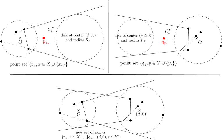
Figure 4. Illustration of the proof of Proposition 3.2. Marked points are drawn in red.

Since $x^{*}$ is extreme in $\chi$, by Lemma 2.4 there exists a point set $\mathcal{P}$ labeled by $X\cup\{x^{*}\}$ with chirotope $\chi$ such that $\mathfrak{p}_{x^{*}}$ is in an unbounded cell $C^{X}_{*}$ of the arrangement of the set of lines $\big{\{}(\mathfrak{p}_{x}\mathfrak{p}_{x^{\prime}}),x,x^{\prime}\in X\}$. Up to rotating and translating this point set, we can assume that $\mathfrak{p}_{x^{*}}$ is on the positive real axis and that the half-line $[\mathfrak{p}_{x^{*}},+\infty)$ does not cross any line $(\mathfrak{p}_{x}\mathfrak{p}_{x^{\prime}})$ with $x,x^{\prime}\in X$. We can further assume that no line $(\mathfrak{p}_{x}\mathfrak{p}_{x^{\prime}})$ with $x,x^{\prime}$ in $X$ is horizontal, since the points are in generic position. We set $R_{X}=\max_{x\in X} \|\mathfrak{p}_{x}\|$. Similarly, there exists a point set $\cal Q$ labeled by $Y\cup\{y^{*}\}$ with chirotope $\xi$ such that $\mathfrak{q}_{y^{*}}$ is on the negative real axis and the half-line $(-\infty,\mathfrak{q}_{x^{*}}]$ does not cross any line $(\mathfrak{q}_{y},\mathfrak{q}_{y^{\prime}})$ with $y,y^{\prime}\in Y$. We set $R_{Y}=\max_{y\in Y} \|\mathfrak{q}_{y}\|$.

Now, let $\mathfrak{p}$ be the point with coordinate $(d,0)$ for some $d>\|\mathfrak{p}_{x^{*}}\|$. The distance between $\mathfrak{p}$ and the union of the lines $(\mathfrak{p}_{x}\mathfrak{p}_{x^{\prime}})$ with $x,x^{\prime}\in X$ goes to infinity as $d$ goes to $+\infty$: indeed it is positive, piecewise affine and could only remain constant if the cell $C_{*}^{X}$ were bounded by horizontal lines (which we ruled out). Thus, for $d$ large enough, say $d>d_{1}$, the disk of radius $R_{Y}$ and center $(d,0)$ entirely lies in $C^{X}_{*}$. Similarly for $d$ large enough, say $d>d_{2}$, the disk of radius $R_{X}$ and center $(-d,0)$ entirely lies in $C^{Y}_{*}$.

We take $d>\max(d_{1},d_{2})$ and consider the point set

$$\big{\{}\mathfrak{p}_{x},x\in X\big{\}}\cup\big{\{}\mathfrak{q}_{y}+(d,0),y\in Y\big{\}},$$

i.e. we take all points $\mathfrak{p}_{x}$ (except $\mathfrak{p}_{x^{*}}$) as they are, and all points $\mathfrak{q}_{y}$ (except $\mathfrak{q}_{y^{*}}$) translated by the vector $(d,0)$. Let $\kappa:(X\cup Y)_{3}\to\{\pm 1\}$ be the chirotope of this point set. Clearly, $\kappa$ is a realizable chirotope, and our goal is now to prove that $\kappa=\chi\mathchoice{\sideset{{}_{x^{*}}}{{}_{y^{*}}}{\operatorname{\textup{\Bowtie}}}}{\sideset{{}_{x^{*}}}{{}_{y^{*}}}{\operatorname{\textup{\Bowtie}}}}{\sideset{{}_{x^{*}}}{{}_{y^{*}}}{\scriptstyle\operatorname{\textup{\Bowtie}}}}{\sideset{{}_{x^{*}}}{{}_{y^{*}}}{\scriptstyle\operatorname{\textup{\Bowtie}}}}\xi$. Obviously,

$$\begin{cases}\kappa(x_{1},x_{2},x_{3})=\chi(x_{1},x_{2},x_{3})\text{ if $x_{1},x_{2},x_{3}$ are all in $X$;}\\ \kappa(y_{1},y_{2},y_{3})=\xi(y_{1},y_{2},y_{3})\text{ if $y_{1},y_{2},y_{3}$ are all in $Y$.}\end{cases}$$

Take $x_{1}$,$x_{2}$ in $X$ and $y$ in $Y$. The point $\mathfrak{q}_{y}+(d,0)$ is in the circle of radius $R_{Y}$ and center $(d,0)$, and is therefore in $C^{X}_{*}$; in other words, $\mathfrak{q}_{y}+(d,0)$ is in the same cell of the arrangement of the lines $\big{\{}(\mathfrak{p}_{x}\mathfrak{p}_{x^{\prime}}),x,x^{\prime}\in X\}$ as $\mathfrak{p}_{x^{*}}$, which implies that $\kappa(x_{1},x_{2},y)=\chi(x_{1},x_{2},x^{*})$.The case where $y_{1}$,$y_{2}$ are in $Y$ and $x$ in $X$ is handled similarly, after translating all the points by $(-d,0)$ (which does not change the chirotope). In this case, $\kappa(x,y_{1},y_{2})=\xi(y^{*},y_{1},y_{2})$. Altogether, this shows that $\kappa=\chi\mathchoice{\sideset{{}_{x^{*}}}{{}_{y^{*}}}{\operatorname{\textup{\Bowtie}}}}{\sideset{{}_{x^{*}}}{{}_{y^{*}}}{\operatorname{\textup{\Bowtie}}}}{\sideset{{}_{x^{*}}}{{}_{y^{*}}}{\scriptstyle\operatorname{\textup{\Bowtie}}}}{\sideset{{}_{x^{*}}}{{}_{y^{*}}}{\scriptstyle\operatorname{\textup{\Bowtie}}}}\xi$, proving that $\chi\mathchoice{\sideset{{}_{x^{*}}}{{}_{y^{*}}}{\operatorname{\textup{\Bowtie}}}}{\sideset{{}_{x^{*}}}{{}_{y^{*}}}{\operatorname{\textup{\Bowtie}}}}{\sideset{{}_{x^{*}}}{{}_{y^{*}}}{\scriptstyle\operatorname{\textup{\Bowtie}}}}{\sideset{{}_{x^{*}}}{{}_{y^{*}}}{\scriptstyle\operatorname{\textup{\Bowtie}}}}\xi$ is realizable. ∎

Propositions 3.1 and 3.2 emphasize the special role of extreme points for the bowtie operation. The following proposition will therefore be useful to iterate bowtie operations.

Proposition 3.3.

Let $\chi$ and $\xi$ be chirotopes on disjoint sets $X\cup\{x^{*}\}$ and $Y\cup\{y^{*}\}$, with $|X|,|Y|\geq 2$, and assume that $x^{*}$ and $y^{*}$ are extreme in $\chi$ and in $\xi$. The extreme elements of $\chi\mathchoice{\sideset{{}_{x^{*}}}{{}_{y^{*}}}{\operatorname{\textup{\Bowtie}}}}{\sideset{{}_{x^{*}}}{{}_{y^{*}}}{\operatorname{\textup{\Bowtie}}}}{\sideset{{}_{x^{*}}}{{}_{y^{*}}}{\scriptstyle\operatorname{\textup{\Bowtie}}}}{\sideset{{}_{x^{*}}}{{}_{y^{*}}}{\scriptstyle\operatorname{\textup{\Bowtie}}}}\xi$ are the extreme elements of $\chi$ other than $x^{*}$ and those of $\xi$ other than $y^{*}$.

Proof.

Let $\kappa\stackrel{{\scriptstyle\text{def}}}{{=}}\chi\mathchoice{\sideset{{}_{x^{*}}}{{}_{y^{*}}}{\operatorname{\textup{\Bowtie}}}}{\sideset{{}_{x^{*}}}{{}_{y^{*}}}{\operatorname{\textup{\Bowtie}}}}{\sideset{{}_{x^{*}}}{{}_{y^{*}}}{\scriptstyle\operatorname{\textup{\Bowtie}}}}{\sideset{{}_{x^{*}}}{{}_{y^{*}}}{\scriptstyle\operatorname{\textup{\Bowtie}}}}\xi$. Let $x_{e}$ be extreme in $\chi$, different from $x^{*}$. There exists $x^{\prime}_{e}\in X$ such that

$$\forall x\in X\cup\{x^{*}\}\setminus\{x_{e},x^{\prime}_{e}\},\quad\kappa(x_{e},x^{\prime}_{e},x)=\chi(x_{e},x^{\prime}_{e},x)=1.$$

If $x^{\prime}_{e}\neq x^{*}$, then for all $y\in Y$ we have $\kappa(x_{e},x_{e}^{\prime},y)=\chi(x_{e},x^{\prime}_{e},x^{*})=1$ and $x_{e}$ is extreme in $\kappa$. If $x^{\prime}_{e}=x^{*}$, then we use the equivalent definition (see 2.3) that $x_{e}$ is extreme in $\chi$ if and only if there exists $x_{e}^{\prime\prime}\in X$ such that

$$\forall x\in X\cup\{x^{*}\}\setminus\{x_{e},x^{\prime\prime}_{e}\},\quad\chi(x_{e},x_{e}^{\prime\prime},x)=-1,$$

and now that $x_{e}^{\prime\prime}\neq x^{*}$ we are back to the previous case, mutatis mutandis. Altogether, the extreme elements of $\chi$ different from $x^{*}$ are extreme for $\kappa$. Similarly, the extreme elements of $\xi$ different from $y^{*}$ are extreme for $\kappa$.

Conversely, let $z_{e}$ be extreme in $\kappa$, and assume w.l.o.g. that $z_{e}\in X$. By definition, there exists $z^{\prime}_{e}\in X\cup Y$ such that for all $z\in X\cup Y\setminus\{z_{e},z^{\prime}_{e}\}$, we have $\kappa(z_{e},z^{\prime}_{e},z)=1$. On the one hand, if $z^{\prime}_{e}\in X$, then $\chi(z_{e},z^{\prime}_{e},x)=\kappa(z_{e},z^{\prime}_{e},x)=1$ for all $x\in X\setminus\{z_{e},z^{\prime}_{e}\}$. In addition, choosing any element $y\in Y$, we have $\chi(z_{e},z^{\prime}_{e},x^{*})=\kappa(z_{e},z^{\prime}_{e},y)=1$, and we recognize that $z_{e}$ is extreme in $\chi$. On the other hand, if $z^{\prime}_{e}\in Y$, then for all $x\in X\setminus\{z_{e}\}$, we have $\chi(z_{e},x^{*},x)=\kappa(z_{e},z^{\prime}_{e},x)=1$, and $z_{e}$ is again extreme in $\chi$. ∎

Propositions 3.1, 3.2 and 3.3 correspond to Proposition 1.1 in the introduction. We conclude this section with two additional results, used respectively in Sections 4 and 7).

For the first result, we recall that a chirotope is called convex if all its elements are extreme. The following statement is an immediate corollary of Proposition 3.3.

Corollary 3.4.

Let $\chi$ be a chirotope with a nontrivial decomposition $\chi=\kappa\mathchoice{\sideset{{}_{x^{*}}}{{}_{y^{*}}}{\operatorname{\textup{\Bowtie}}}}{\sideset{{}_{x^{*}}}{{}_{y^{*}}}{\operatorname{\textup{\Bowtie}}}}{\sideset{{}_{x^{*}}}{{}_{y^{*}}}{\scriptstyle\operatorname{\textup{\Bowtie}}}}{\sideset{{}_{x^{*}}}{{}_{y^{*}}}{\scriptstyle\operatorname{\textup{\Bowtie}}}}\xi$. The chirotope $\chi$ is convex if and only if both $\kappa$ and $\xi$ are convex.

3.2. Modules

Let us now consider reversing the bowtie operation: given a chirotope $\kappa$ on ground set $Z$, we want a bipartition $X\uplus Y$ of $Z$, and chirotopes $\chi$ and $\xi$ on ground sets $X\cup\{x^{*}\}$ and $Y\cup\{y^{*}\}$ (for new elements $x^{*}$ and $y^{*}$) such that $\kappa=\chi\mathchoice{\sideset{{}_{x^{*}}}{{}_{y^{*}}}{\operatorname{\textup{\Bowtie}}}}{\sideset{{}_{x^{*}}}{{}_{y^{*}}}{\operatorname{\textup{\Bowtie}}}}{\sideset{{}_{x^{*}}}{{}_{y^{*}}}{\scriptstyle\operatorname{\textup{\Bowtie}}}}{\sideset{{}_{x^{*}}}{{}_{y^{*}}}{\scriptstyle\operatorname{\textup{\Bowtie}}}}\xi$. We call such a decomposition $\kappa=\chi\mathchoice{\sideset{{}_{x^{*}}}{{}_{y^{*}}}{\operatorname{\textup{\Bowtie}}}}{\sideset{{}_{x^{*}}}{{}_{y^{*}}}{\operatorname{\textup{\Bowtie}}}}{\sideset{{}_{x^{*}}}{{}_{y^{*}}}{\scriptstyle\operatorname{\textup{\Bowtie}}}}{\sideset{{}_{x^{*}}}{{}_{y^{*}}}{\scriptstyle\operatorname{\textup{\Bowtie}}}}\xi$ a bowtie decomposition of $\kappa$.

These considerations lead naturally to the following notion.

Definition 3.5.

A subset $X\subseteq Z$ is a module of a chirotope $\kappa$ on $Z$ if for every $x,x^{\prime}\in X$ and $y,y^{\prime}\in Z\setminus X$, one has $\kappa(x,x^{\prime},y)=\kappa(x,x^{\prime},y^{\prime})$ and $\kappa(x,y,y^{\prime})=\kappa(x^{\prime},y,y^{\prime})$. The bipartition $\{X,Z\setminus X\}$ of $Z$ is called a modular bipartition of $\kappa$.

Note that $X$ is a module of $\kappa$ if and only if $Z\setminus X$ is a module of $\kappa$. The notion of module is chosen so that the following observation holds.

Observation 3.6.

Let $\kappa$ be a chirotope on ground set $Z$ and $\{X,Y\}$ a bipartition of $Z$. There exist chirotopes $\chi$ and $\xi$ on disjoint ground sets $X\cup\{x^{*}\}$ and $Y\cup\{y^{*}\}$ such that $\kappa=\chi\mathchoice{\sideset{{}_{x^{*}}}{{}_{y^{*}}}{\operatorname{\textup{\Bowtie}}}}{\sideset{{}_{x^{*}}}{{}_{y^{*}}}{\operatorname{\textup{\Bowtie}}}}{\sideset{{}_{x^{*}}}{{}_{y^{*}}}{\scriptstyle\operatorname{\textup{\Bowtie}}}}{\sideset{{}_{x^{*}}}{{}_{y^{*}}}{\scriptstyle\operatorname{\textup{\Bowtie}}}}\xi$ if and only if $X$ is a module of $\kappa$. Moreover, when the chirotopes $\chi$ and $\xi$ exist, they are unique up to the choice of the labels for $x^{*}$ and $y^{*}$.

Remark 3.7.

If one of $X$ or $Y$ has size at most $1$, then $\{X,Y\}$ is always a modular bipartition of $\kappa$, but the size of $\chi$ or $\xi$ is at least that of $\kappa$. We refer to such modular bipartitions, modules or bowtie decomposition as trivial. Note that in a nontrivial bipartition $\{X,Y\}$ of $\kappa$, both $X$ and $Y$ have size at least $2$, which implies in particular that both $\chi$ and $\xi$ in the decomposition $\kappa=\chi\mathchoice{\sideset{{}_{x^{*}}}{{}_{y^{*}}}{\operatorname{\textup{\Bowtie}}}}{\sideset{{}_{x^{*}}}{{}_{y^{*}}}{\operatorname{\textup{\Bowtie}}}}{\sideset{{}_{x^{*}}}{{}_{y^{*}}}{\scriptstyle\operatorname{\textup{\Bowtie}}}}{\sideset{{}_{x^{*}}}{{}_{y^{*}}}{\scriptstyle\operatorname{\textup{\Bowtie}}}}\xi$ have ground sets of size at least $3$.

Remark 3.8.

When $\kappa$ is realizable, its nontrivial modular bipartitions have a simple geometric interpretation: $X$ is a nontrivial module if in a realization of $\kappa$, no line through two points with labels in $X$ separates two points with labels outside $X$, and conversely no line through two points with labels outside $X$ separates two points with labels in $X$. This explains the connection with the notion of mutually avoiding sets given in the introduction: a modular bipartition is a pair of mutually avoiding sets covering the whole chirotope.

The next lemma studies the stability of modules under intersection, and will be useful in the next section.

Lemma 3.9.

Let $X_{1},X_{2}$ be two modules of a chirotope $\kappa$ with ground set $Z$. If $X_{1}\cup X_{2}\neq Z$, then $X_{1}\cap X_{2}$ is a module of $\kappa$.

Proof.

Let $x,x^{\prime}\in X_{1}\cap X_{2}$ and $y,y^{\prime}\in Z\setminus(X_{1}\cap X_{2})$. Let $p\in Z\setminus(X_{1}\cup X_{2})$. Since $y$ is outside $X_{1}\cap X_{2}$, the set $\{y,p\}$ is disjoint from $X_{1}$ or from $X_{2}$. In either case, we have $\kappa(x,x^{\prime},y)=\kappa(x,x^{\prime},p)$. A symmetric argument yields $\kappa(x,x^{\prime},p)=\kappa(x,x^{\prime},y^{\prime})$, so we have $\kappa(x,x^{\prime},y)=\kappa(x,x^{\prime},y^{\prime})$.

It remains to argue that $\kappa(x,y,y^{\prime})=\kappa(x^{\prime},y,y^{\prime})$. This is clear if both $y$ and $y^{\prime}$ are outside of $X_{1}$, as $X_{1}$ is a module, so assume otherwise. Suppose, without loss of generality, that $y\in X_{1}\setminus X_{2}$, and $y^{\prime}\in X_{2}\setminus X_{1}$. As $x,x^{\prime},y\in X_{1}$ and $p,y^{\prime}\notin X_{1}$ we have $\kappa(x,y,y^{\prime})=\kappa(x,y,p)$ and $\kappa(x^{\prime},y,y^{\prime})=\kappa(x^{\prime},y,p)$. As $p,y\notin X_{2}$ and $x,x^{\prime}\in X_{2}$, $\kappa(x,y,p)=\kappa(x^{\prime},y,p)$. Altogether, we get $\kappa(x,y,y^{\prime})=\kappa(x^{\prime},y,y^{\prime})$ as desired. ∎

Remark 3.10.

The condition $X_{1}\cup X_{2}\neq Z$ in Lemma 3.9 is indeed necessary. To see this, consider the chirotope induced by the following point set, where $X_{1}=\{a,b,x,y\}$ and $X_{2}=\{c,d,x,y\}$ are nontrivial modules but $X_{1}\cap X_{2}=\{x,y\}$ is not a module:

3.3. Commutativity and associativity

Proposition 3.11.

Let $\chi$, $\xi$, $\kappa$ be chirotopes on disjoint ground sets $X\cup\{x^{*}\}$, $Y\cup\{y_{1}^{*},y_{2}^{*}\}$ and $Z\cup\{z^{*}\}$, with $|X|,|Z|\geq 2,|Y|\geq 1$. If the starred elements are extreme in their respective chirotopes, then $\chi\mathchoice{\sideset{{}_{x^{*}}}{{}_{y_{1}^{*}}}{\operatorname{\textup{\Bowtie}}}}{\sideset{{}_{x^{*}}}{{}_{y_{1}^{*}}}{\operatorname{\textup{\Bowtie}}}}{\sideset{{}_{x^{*}}}{{}_{y_{1}^{*}}}{\scriptstyle\operatorname{\textup{\Bowtie}}}}{\sideset{{}_{x^{*}}}{{}_{y_{1}^{*}}}{\scriptstyle\operatorname{\textup{\Bowtie}}}}\xi=\xi\mathchoice{\sideset{{}_{y_{1}^{*}}}{{}_{x^{*}}}{\operatorname{\textup{\Bowtie}}}}{\sideset{{}_{y_{1}^{*}}}{{}_{x^{*}}}{\operatorname{\textup{\Bowtie}}}}{\sideset{{}_{y_{1}^{*}}}{{}_{x^{*}}}{\scriptstyle\operatorname{\textup{\Bowtie}}}}{\sideset{{}_{y_{1}^{*}}}{{}_{x^{*}}}{\scriptstyle\operatorname{\textup{\Bowtie}}}}\chi$ and $(\chi\mathchoice{\sideset{{}_{x^{*}}}{{}_{y_{1}^{*}}}{\operatorname{\textup{\Bowtie}}}}{\sideset{{}_{x^{*}}}{{}_{y_{1}^{*}}}{\operatorname{\textup{\Bowtie}}}}{\sideset{{}_{x^{*}}}{{}_{y_{1}^{*}}}{\scriptstyle\operatorname{\textup{\Bowtie}}}}{\sideset{{}_{x^{*}}}{{}_{y_{1}^{*}}}{\scriptstyle\operatorname{\textup{\Bowtie}}}}\xi)\mathchoice{\sideset{{}_{y_{2}^{*}}}{{}_{z^{*}}}{\operatorname{\textup{\Bowtie}}}}{\sideset{{}_{y_{2}^{*}}}{{}_{z^{*}}}{\operatorname{\textup{\Bowtie}}}}{\sideset{{}_{y_{2}^{*}}}{{}_{z^{*}}}{\scriptstyle\operatorname{\textup{\Bowtie}}}}{\sideset{{}_{y_{2}^{*}}}{{}_{z^{*}}}{\scriptstyle\operatorname{\textup{\Bowtie}}}}\kappa=\chi\mathchoice{\sideset{{}_{x^{*}}}{{}_{y_{1}^{*}}}{\operatorname{\textup{\Bowtie}}}}{\sideset{{}_{x^{*}}}{{}_{y_{1}^{*}}}{\operatorname{\textup{\Bowtie}}}}{\sideset{{}_{x^{*}}}{{}_{y_{1}^{*}}}{\scriptstyle\operatorname{\textup{\Bowtie}}}}{\sideset{{}_{x^{*}}}{{}_{y_{1}^{*}}}{\scriptstyle\operatorname{\textup{\Bowtie}}}}(\xi\mathchoice{\sideset{{}_{y_{2}^{*}}}{{}_{z^{*}}}{\operatorname{\textup{\Bowtie}}}}{\sideset{{}_{y_{2}^{*}}}{{}_{z^{*}}}{\operatorname{\textup{\Bowtie}}}}{\sideset{{}_{y_{2}^{*}}}{{}_{z^{*}}}{\scriptstyle\operatorname{\textup{\Bowtie}}}}{\sideset{{}_{y_{2}^{*}}}{{}_{z^{*}}}{\scriptstyle\operatorname{\textup{\Bowtie}}}}\kappa)$.

Proof.

The commutativity comes from the symmetry of the definition of the bowtie operation. Let us focus on the associativity condition. Let $\lambda_{1}=(\chi\mathchoice{\sideset{{}_{x^{*}}}{{}_{y_{1}^{*}}}{\operatorname{\textup{\Bowtie}}}}{\sideset{{}_{x^{*}}}{{}_{y_{1}^{*}}}{\operatorname{\textup{\Bowtie}}}}{\sideset{{}_{x^{*}}}{{}_{y_{1}^{*}}}{\scriptstyle\operatorname{\textup{\Bowtie}}}}{\sideset{{}_{x^{*}}}{{}_{y_{1}^{*}}}{\scriptstyle\operatorname{\textup{\Bowtie}}}}\xi)\mathchoice{\sideset{{}_{y_{2}^{*}}}{{}_{z^{*}}}{\operatorname{\textup{\Bowtie}}}}{\sideset{{}_{y_{2}^{*}}}{{}_{z^{*}}}{\operatorname{\textup{\Bowtie}}}}{\sideset{{}_{y_{2}^{*}}}{{}_{z^{*}}}{\scriptstyle\operatorname{\textup{\Bowtie}}}}{\sideset{{}_{y_{2}^{*}}}{{}_{z^{*}}}{\scriptstyle\operatorname{\textup{\Bowtie}}}}\kappa$, and $\lambda_{2}=\chi\mathchoice{\sideset{{}_{x^{*}}}{{}_{y_{1}^{*}}}{\operatorname{\textup{\Bowtie}}}}{\sideset{{}_{x^{*}}}{{}_{y_{1}^{*}}}{\operatorname{\textup{\Bowtie}}}}{\sideset{{}_{x^{*}}}{{}_{y_{1}^{*}}}{\scriptstyle\operatorname{\textup{\Bowtie}}}}{\sideset{{}_{x^{*}}}{{}_{y_{1}^{*}}}{\scriptstyle\operatorname{\textup{\Bowtie}}}}(\xi\mathchoice{\sideset{{}_{y_{2}^{*}}}{{}_{z^{*}}}{\operatorname{\textup{\Bowtie}}}}{\sideset{{}_{y_{2}^{*}}}{{}_{z^{*}}}{\operatorname{\textup{\Bowtie}}}}{\sideset{{}_{y_{2}^{*}}}{{}_{z^{*}}}{\scriptstyle\operatorname{\textup{\Bowtie}}}}{\sideset{{}_{y_{2}^{*}}}{{}_{z^{*}}}{\scriptstyle\operatorname{\textup{\Bowtie}}}}\kappa)$, which are both sign functions on $X\cup Y\cup Z$. Let us take three elements $t,u,v$ in $X\cup Y\cup Z$. Suppose first that $t,u,v$ all belong to the set $X$. Then by definition of the bowtie $\lambda_{1}(t,u,v)=[(\chi\mathchoice{\sideset{{}_{x^{*}}}{{}_{y_{1}^{*}}}{\operatorname{\textup{\Bowtie}}}}{\sideset{{}_{x^{*}}}{{}_{y_{1}^{*}}}{\operatorname{\textup{\Bowtie}}}}{\sideset{{}_{x^{*}}}{{}_{y_{1}^{*}}}{\scriptstyle\operatorname{\textup{\Bowtie}}}}{\sideset{{}_{x^{*}}}{{}_{y_{1}^{*}}}{\scriptstyle\operatorname{\textup{\Bowtie}}}}\xi)\mathchoice{\sideset{{}_{y_{2}^{*}}}{{}_{z^{*}}}{\operatorname{\textup{\Bowtie}}}}{\sideset{{}_{y_{2}^{*}}}{{}_{z^{*}}}{\operatorname{\textup{\Bowtie}}}}{\sideset{{}_{y_{2}^{*}}}{{}_{z^{*}}}{\scriptstyle\operatorname{\textup{\Bowtie}}}}{\sideset{{}_{y_{2}^{*}}}{{}_{z^{*}}}{\scriptstyle\operatorname{\textup{\Bowtie}}}}\kappa](t,u,v)=(\chi\mathchoice{\sideset{{}_{x^{*}}}{{}_{y_{1}^{*}}}{\operatorname{\textup{\Bowtie}}}}{\sideset{{}_{x^{*}}}{{}_{y_{1}^{*}}}{\operatorname{\textup{\Bowtie}}}}{\sideset{{}_{x^{*}}}{{}_{y_{1}^{*}}}{\scriptstyle\operatorname{\textup{\Bowtie}}}}{\sideset{{}_{x^{*}}}{{}_{y_{1}^{*}}}{\scriptstyle\operatorname{\textup{\Bowtie}}}}\xi)(t,u,v)=\chi(t,u,v)$, and similarly $\lambda_{2}(t,u,v)=\chi(t,u,v)$. The cases where $t,u,v$ are all in $Y$, or all in $Z$, are similar. If $t,u,v$ all belong to different sets among $X$, $Y$ and $Z$, for example if $t\in X$, $u\in Y$, $v\in Z$, then $\lambda_{1}(t,u,v)=(\chi\mathchoice{\sideset{{}_{x^{*}}}{{}_{y_{1}^{*}}}{\operatorname{\textup{\Bowtie}}}}{\sideset{{}_{x^{*}}}{{}_{y_{1}^{*}}}{\operatorname{\textup{\Bowtie}}}}{\sideset{{}_{x^{*}}}{{}_{y_{1}^{*}}}{\scriptstyle\operatorname{\textup{\Bowtie}}}}{\sideset{{}_{x^{*}}}{{}_{y_{1}^{*}}}{\scriptstyle\operatorname{\textup{\Bowtie}}}}\xi)(t,u,y_{2}^{*})=\xi(y_{1}^{*},u,y_{2}^{*})$, and $\lambda_{2}(t,u,v)=(\xi\mathchoice{\sideset{{}_{y_{2}^{*}}}{{}_{z^{*}}}{\operatorname{\textup{\Bowtie}}}}{\sideset{{}_{y_{2}^{*}}}{{}_{z^{*}}}{\operatorname{\textup{\Bowtie}}}}{\sideset{{}_{y_{2}^{*}}}{{}_{z^{*}}}{\scriptstyle\operatorname{\textup{\Bowtie}}}}{\sideset{{}_{y_{2}^{*}}}{{}_{z^{*}}}{\scriptstyle\operatorname{\textup{\Bowtie}}}}\kappa)(y_{1}^{*},u,v)=\xi(y_{1}^{*},u,y_{2}^{*})$. The final cases where one element is isolated in one set are very similar. ∎

Remark 3.12.

When using the associativity of bowties, one should pay particular attention to the ground sets of the chirotopes at play. For instance, with the notation of Proposition 3.11, writing $(\xi\mathchoice{\sideset{{}_{y_{1}^{*}}}{{}_{x^{*}}}{\operatorname{\textup{\Bowtie}}}}{\sideset{{}_{y_{1}^{*}}}{{}_{x^{*}}}{\operatorname{\textup{\Bowtie}}}}{\sideset{{}_{y_{1}^{*}}}{{}_{x^{*}}}{\scriptstyle\operatorname{\textup{\Bowtie}}}}{\sideset{{}_{y_{1}^{*}}}{{}_{x^{*}}}{\scriptstyle\operatorname{\textup{\Bowtie}}}}\chi)\mathchoice{\sideset{{}_{y_{2}^{*}}}{{}_{z^{*}}}{\operatorname{\textup{\Bowtie}}}}{\sideset{{}_{y_{2}^{*}}}{{}_{z^{*}}}{\operatorname{\textup{\Bowtie}}}}{\sideset{{}_{y_{2}^{*}}}{{}_{z^{*}}}{\scriptstyle\operatorname{\textup{\Bowtie}}}}{\sideset{{}_{y_{2}^{*}}}{{}_{z^{*}}}{\scriptstyle\operatorname{\textup{\Bowtie}}}}\kappa=\xi\mathchoice{\sideset{{}_{y_{1}^{*}}}{{}_{x^{*}}}{\operatorname{\textup{\Bowtie}}}}{\sideset{{}_{y_{1}^{*}}}{{}_{x^{*}}}{\operatorname{\textup{\Bowtie}}}}{\sideset{{}_{y_{1}^{*}}}{{}_{x^{*}}}{\scriptstyle\operatorname{\textup{\Bowtie}}}}{\sideset{{}_{y_{1}^{*}}}{{}_{x^{*}}}{\scriptstyle\operatorname{\textup{\Bowtie}}}}(\chi\mathchoice{\sideset{{}_{y_{2}^{*}}}{{}_{z^{*}}}{\operatorname{\textup{\Bowtie}}}}{\sideset{{}_{y_{2}^{*}}}{{}_{z^{*}}}{\operatorname{\textup{\Bowtie}}}}{\sideset{{}_{y_{2}^{*}}}{{}_{z^{*}}}{\scriptstyle\operatorname{\textup{\Bowtie}}}}{\sideset{{}_{y_{2}^{*}}}{{}_{z^{*}}}{\scriptstyle\operatorname{\textup{\Bowtie}}}}\kappa)$ does not make sense, as in the right-hand term $y_{2}^{*}$ does not belong to the ground set of $\chi$ (even though the left-hand term is well-defined).

4. Existence and uniqueness of the canonical chirotope tree

We now examine how iterated bowtie products can be described and manipulated via trees.

4.1. Chirotope trees and their chirotopes

We first recall some definitions from the introduction. A chirotope tree is a tree whose nodes are decorated with chirotopes on disjoint ground sets, each of size at least $3$, and whose edges select an element in the ground set of each of their nodes in a way that (i) no element is selected more than once, and (ii) each selected element is extreme in its chirotope. To be complete, let us stress out that all trees are graph-theoretical trees $T=(V_{T},E_{T})$, i.e. simple connected graphs without cycles, and call them trees. In particular, trees are always unrooted and unordered (neighbors of a given node are not ordered).

Given a chirotope tree $T$, one associates to it a sign function $\chi_{T}$ on $\bigcup_{w\in V_{T}}X_{w}$ defined by

(12) $$\chi_{T}(x,y,z)\stackrel{{\scriptstyle\text{def}}}{{=}}\chi_{v}(R(x,v),R(y,v),R(z,v)),$$

where $v$ is the branching point of the paths from $x$ to $y$, $y$ to $z$ and $x$ to $z$, and $R(x,v)$, $R(y,v)$ and $R(z,v)$ the representatives of $x$, $y$ and $z$ in $v$ (i.e. the proxy points of $\chi_{v}$ to which the path going form $v$ to the nodes containing $x$, $y$ and $z$ are attached). If two or more elements among $x$, $y$ and $z$ belong to the same node, then $v$ is taken to be this node, and we use the convention that $R(s,v)=s$ for $s$ in $X_{v}$.

It is easy to see that this defines a sign function on $\bigcup_{w\in V_{T}}X_{w}$; we now prove Proposition 1.2, which state that it is always a chirotope, and furthermore realizable if all chirotopes decorating the nodes of $T$ are realizable. Let us start with a lemma.

Lemma 4.1.

Let $T$ be a chirotope tree and $e=\{v_{1},v_{2}\}$ an edge of $T$, and let $s_{1}$ and $s_{2}$ be the elements selected by $e$ in $v_{1}$ and $v_{2}$ respectively. If $T_{1}$ and $T_{2}$ denote the two chirotope trees obtained by removing $e$ from $T$, with $v_{i}\in T_{i}$, then $\chi_{T}=\chi_{T_{1}}\mathchoice{\sideset{{}_{s_{1}}}{{}_{s_{2}}}{\operatorname{\textup{\Bowtie}}}}{\sideset{{}_{s_{1}}}{{}_{s_{2}}}{\operatorname{\textup{\Bowtie}}}}{\sideset{{}_{s_{1}}}{{}_{s_{2}}}{\scriptstyle\operatorname{\textup{\Bowtie}}}}{\sideset{{}_{s_{1}}}{{}_{s_{2}}}{\scriptstyle\operatorname{\textup{\Bowtie}}}}\chi_{T_{2}}$.

Proof.

First, we note that after the removal of $e$, $s_{1}$ and $s_{2}$ are no longer proxies in $T_{1}$ and $T_{2}$, and the bowtie $\kappa=\chi_{T_{1}}\mathchoice{\sideset{{}_{s_{1}}}{{}_{s_{2}}}{\operatorname{\textup{\Bowtie}}}}{\sideset{{}_{s_{1}}}{{}_{s_{2}}}{\operatorname{\textup{\Bowtie}}}}{\sideset{{}_{s_{1}}}{{}_{s_{2}}}{\scriptstyle\operatorname{\textup{\Bowtie}}}}{\sideset{{}_{s_{1}}}{{}_{s_{2}}}{\scriptstyle\operatorname{\textup{\Bowtie}}}}\chi_{T_{2}}$ is thus well-defined.

It remains to check that $\kappa=\chi_{T}$. Let $X$ denote the ground set of $\kappa$. This set decomposes into $X=X_{1}\uplus X_{2}$, where $X_{i}\uplus\{s_{i}\}$ is the ground set of $T_{i}$, for $i=1,2$. It is easy to check that given $x\in X$ and a node $v\in T$, we have

$$R_{T}(x,v)=\left\{\begin{array}[]{ll}R_{T_{1}}(x,v)&\text{if }v\in T_{1}\text{ and }x\in X_{1},\\ R_{T_{1}}(s_{1},v)&\text{if }v\in T_{1}\text{ and }x\in X_{2},\\ R_{T_{2}}(s_{2},v)&\text{if }v\in T_{2}\text{ and }x\in X_{1},\\ R_{T_{2}}(x,v)&\text{if }v\in T_{2}\text{ and }x\in X_{2}.\\ \end{array}\right.$$

From this, it is easy to check that $\kappa(x,y,z)=\chi_{T}(x,y,z)$ for any $x,y,z$ in $X$. For instance, if $x,y\in X_{1}$ and $z\in X_{2}$, then the node $v\stackrel{{\scriptstyle\text{def}}}{{=}}v(x,y,z)$ lies in $T_{1}$ and

$$R_{T}(x,v)=R_{T_{1}}(x,v),\qquad R_{T}(y,v)=R_{T_{1}}(y,v),\qquad R_{T}(z,v)=R_{T_{1}}(s_{1},v).$$

We therefore get

$$\chi_{T}(x,y,z)=\chi_{v}(R_{T_{1}}(x,v),R_{T_{1}}(y,v),R_{T_{1}}(s_{1},v))=\chi_{T_{1}}(x,y,s_{1})=\kappa(x,y,z),$$

where the middle equality uses Eq. 12 for $T_{1}$, and the last equality follows from the definition of the bowtie operation (Eq. 4). Other cases (two elements in $X_{2}$ and one in $X_{1}$, or the three elements in the same set) are similar or easier. This proves $\kappa=\chi_{T}$ as wanted. ∎

The proof of Proposition 1.2 is now a straightforward induction using Lemma 4.1 and the fact that the bowtie of two (realizable) chirotopes whose starred elements are extreme is a (realizable) chirotope (see Propositions 3.1, 3.2 and 3.3). Iterating this lemma, we can actually compute $\chi_{T}$ starting from the sign functions $\chi_{v}$ and iterating bowtie operations. For example, if $T$ is the chirotope tree on Fig. 5, we have

(13) $$\chi_{T}=(\chi_{1}\mathchoice{\sideset{{}_{x_{1}^{*}}}{{}_{x_{2}^{*}}}{\operatorname{\textup{\Bowtie}}}}{\sideset{{}_{x_{1}^{*}}}{{}_{x_{2}^{*}}}{\operatorname{\textup{\Bowtie}}}}{\sideset{{}_{x_{1}^{*}}}{{}_{x_{2}^{*}}}{\scriptstyle\operatorname{\textup{\Bowtie}}}}{\sideset{{}_{x_{1}^{*}}}{{}_{x_{2}^{*}}}{\scriptstyle\operatorname{\textup{\Bowtie}}}}(\chi_{2}\mathchoice{\sideset{{}_{y_{2}^{*}}}{{}_{x_{3}^{*}}}{\operatorname{\textup{\Bowtie}}}}{\sideset{{}_{y_{2}^{*}}}{{}_{x_{3}^{*}}}{\operatorname{\textup{\Bowtie}}}}{\sideset{{}_{y_{2}^{*}}}{{}_{x_{3}^{*}}}{\scriptstyle\operatorname{\textup{\Bowtie}}}}{\sideset{{}_{y_{2}^{*}}}{{}_{x_{3}^{*}}}{\scriptstyle\operatorname{\textup{\Bowtie}}}}\chi_{3}))\mathchoice{\sideset{{}_{z_{2}^{*}}}{{}_{x_{4}^{*}}}{\operatorname{\textup{\Bowtie}}}}{\sideset{{}_{z_{2}^{*}}}{{}_{x_{4}^{*}}}{\operatorname{\textup{\Bowtie}}}}{\sideset{{}_{z_{2}^{*}}}{{}_{x_{4}^{*}}}{\scriptstyle\operatorname{\textup{\Bowtie}}}}{\sideset{{}_{z_{2}^{*}}}{{}_{x_{4}^{*}}}{\scriptstyle\operatorname{\textup{\Bowtie}}}}\chi_{4}.$$

Figure 5. An example of chirotope tree.

We note that, when iterating Lemma 4.1, we can choose at each step which edge plays the role of $e$ in the lemma. This leads to different expressions of $\chi_{T}$ as a sequence of bowtie operations. Considering again the chirotope tree $T$ on Fig. 5, we could have written

(14) $$\chi_{T}=\chi_{1}\mathchoice{\sideset{{}_{x_{1}^{*}}}{{}_{x_{2}^{*}}}{\operatorname{\textup{\Bowtie}}}}{\sideset{{}_{x_{1}^{*}}}{{}_{x_{2}^{*}}}{\operatorname{\textup{\Bowtie}}}}{\sideset{{}_{x_{1}^{*}}}{{}_{x_{2}^{*}}}{\scriptstyle\operatorname{\textup{\Bowtie}}}}{\sideset{{}_{x_{1}^{*}}}{{}_{x_{2}^{*}}}{\scriptstyle\operatorname{\textup{\Bowtie}}}}((\chi_{2}\mathchoice{\sideset{{}_{z_{2}^{*}}}{{}_{x_{4}^{*}}}{\operatorname{\textup{\Bowtie}}}}{\sideset{{}_{z_{2}^{*}}}{{}_{x_{4}^{*}}}{\operatorname{\textup{\Bowtie}}}}{\sideset{{}_{z_{2}^{*}}}{{}_{x_{4}^{*}}}{\scriptstyle\operatorname{\textup{\Bowtie}}}}{\sideset{{}_{z_{2}^{*}}}{{}_{x_{4}^{*}}}{\scriptstyle\operatorname{\textup{\Bowtie}}}}\chi_{4})\mathchoice{\sideset{{}_{y_{2}^{*}}}{{}_{x_{3}^{*}}}{\operatorname{\textup{\Bowtie}}}}{\sideset{{}_{y_{2}^{*}}}{{}_{x_{3}^{*}}}{\operatorname{\textup{\Bowtie}}}}{\sideset{{}_{y_{2}^{*}}}{{}_{x_{3}^{*}}}{\scriptstyle\operatorname{\textup{\Bowtie}}}}{\sideset{{}_{y_{2}^{*}}}{{}_{x_{3}^{*}}}{\scriptstyle\operatorname{\textup{\Bowtie}}}}\chi_{3})$$

The equivalence of Eqs. 13 and 14 follows from the commutativity and associativity properties of the bowtie operation (Proposition 3.11).

Remark 4.2.

From Eq. 12, it follows immediately that the sign function $\chi_{T}$ associated to a chirotope tree $T$ does not depend on the labels of its proxies. Accordingly, in the following, we consider chirotope trees up to relabeling of their proxies.

4.2. Two Operations on chirotope trees

We now adapt two standard operations on trees (edge contraction and vertex split) for chirotope trees in a way that leaves the associated chirotopes invariant.

4.2.1. Contraction

Definition 4.3.

Let $T$ be a chirotope tree and $e=\{v,v^{\prime}\}$ be an edge in $T$ that selects $s^{*}$ and $t^{*}$ in $\chi_{v}$ and $\chi_{v^{\prime}}$, respectively. The contraction of $e$ in $T$ is the tree $T^{\prime}$ obtained from $T$ by merging the nodes $v$ and $v^{\prime}$ into a new node $v_{new}$, decorated with the chirotope $\chi_{new}\stackrel{{\scriptstyle\text{def}}}{{=}}\chi_{v}\mathchoice{\sideset{{}_{s^{*}}}{{}_{t^{*}}}{\operatorname{\textup{\Bowtie}}}}{\sideset{{}_{s^{*}}}{{}_{t^{*}}}{\operatorname{\textup{\Bowtie}}}}{\sideset{{}_{s^{*}}}{{}_{t^{*}}}{\scriptstyle\operatorname{\textup{\Bowtie}}}}{\sideset{{}_{s^{*}}}{{}_{t^{*}}}{\scriptstyle\operatorname{\textup{\Bowtie}}}}\chi_{v^{\prime}}$. We denote this transformation by $T\xrightarrow{e}T^{\prime}$.

Note that, by Propositions 3.1 and 3.2, $\chi_{new}$ is a chirotope, and is realizable if both $\chi_{v}$ and $\chi_{v^{\prime}}$ are realizable. Furthermore, by Proposition 3.3, the extreme elements of $\chi_{v}$ and $\chi_{v^{\prime}}$ different from $s^{*}$ and $t^{*}$ are extreme elements of $\chi_{new}$ so that the proxy elements corresponding to other edges of $T$ are still extreme in their respective chirotopes in $T^{\prime}$; it follows that $T^{\prime}$ is indeed a chirotope tree.

Example 4.4.

Here is an example of a contraction of an edge in a chirotope tree (with $\chi=\kappa\mathchoice{\sideset{{}_{s^{*}}}{{}_{t^{*}}}{\operatorname{\textup{\Bowtie}}}}{\sideset{{}_{s^{*}}}{{}_{t^{*}}}{\operatorname{\textup{\Bowtie}}}}{\sideset{{}_{s^{*}}}{{}_{t^{*}}}{\scriptstyle\operatorname{\textup{\Bowtie}}}}{\sideset{{}_{s^{*}}}{{}_{t^{*}}}{\scriptstyle\operatorname{\textup{\Bowtie}}}}\xi$).

$\xrightarrow[]{(s^{*},t^{*})}$  

4.2.2. Split

Definition 4.5.

Let $T$ be a chirotope tree with a node $v_{0}$ whose decoration $\chi_{v_{0}}=\chi$ has a nontrivial bowtie decomposition $\chi=\kappa\mathchoice{\sideset{{}_{s^{*}}}{{}_{t^{*}}}{\operatorname{\textup{\Bowtie}}}}{\sideset{{}_{s^{*}}}{{}_{t^{*}}}{\operatorname{\textup{\Bowtie}}}}{\sideset{{}_{s^{*}}}{{}_{t^{*}}}{\scriptstyle\operatorname{\textup{\Bowtie}}}}{\sideset{{}_{s^{*}}}{{}_{t^{*}}}{\scriptstyle\operatorname{\textup{\Bowtie}}}}\xi$. The split of $T$ according to $\chi=\kappa\mathchoice{\sideset{{}_{s^{*}}}{{}_{t^{*}}}{\operatorname{\textup{\Bowtie}}}}{\sideset{{}_{s^{*}}}{{}_{t^{*}}}{\operatorname{\textup{\Bowtie}}}}{\sideset{{}_{s^{*}}}{{}_{t^{*}}}{\scriptstyle\operatorname{\textup{\Bowtie}}}}{\sideset{{}_{s^{*}}}{{}_{t^{*}}}{\scriptstyle\operatorname{\textup{\Bowtie}}}}\xi$ is the tree $T^{\prime}$ obtained from $T$ by replacing $v_{0}$ by two nodes $v_{1}$ and $v_{2}$ that are decorated by $\kappa$ and $\xi$, respectively, and form an edge selecting $s^{*}$ in $v_{1}$ and $t^{*}$ in $v_{2}$. Denote this transformation by $T\xrightarrow[\kappa\mathchoice{\sideset{{}_{s^{*}}}{{}_{t^{*}}}{\operatorname{\textup{\Bowtie}}}}{\sideset{{}_{s^{*}}}{{}_{t^{*}}}{\operatorname{\textup{\Bowtie}}}}{\sideset{{}_{s^{*}}}{{}_{t^{*}}}{\scriptstyle\operatorname{\textup{\Bowtie}}}}{\sideset{{}_{s^{*}}}{{}_{t^{*}}}{\scriptstyle\operatorname{\textup{\Bowtie}}}}\xi]{\chi}T^{\prime}$.

Note that for any edge $e=\{s^{e}_{v_{0}},s^{e}_{w}\}$ connecting $v_{0}$ to another vertex $w$ in $T$, the element $s^{e}_{v_{0}}$ belongs to the ground set of either $\kappa$ or $\xi$. Therefore, $e$ is naturally seen as an edge of $T^{\prime}$, connecting either $v_{1}$ or $v_{2}$ to $w$, depending on the set in which $s^{e}_{v_{0}}$ lies.

Example 4.6.

Here is an example of a split of a tree according to the bowtie decomposition $\chi=\kappa\mathchoice{\sideset{{}_{s^{*}}}{{}_{t^{*}}}{\operatorname{\textup{\Bowtie}}}}{\sideset{{}_{s^{*}}}{{}_{t^{*}}}{\operatorname{\textup{\Bowtie}}}}{\sideset{{}_{s^{*}}}{{}_{t^{*}}}{\scriptstyle\operatorname{\textup{\Bowtie}}}}{\sideset{{}_{s^{*}}}{{}_{t^{*}}}{\scriptstyle\operatorname{\textup{\Bowtie}}}}\xi$.

$\xrightarrow[\kappa\mathchoice{\sideset{{}_{s^{*}}}{{}_{t^{*}}}{\operatorname{\textup{\Bowtie}}}}{\sideset{{}_{s^{*}}}{{}_{t^{*}}}{\operatorname{\textup{\Bowtie}}}}{\sideset{{}_{s^{*}}}{{}_{t^{*}}}{\scriptstyle\operatorname{\textup{\Bowtie}}}}{\sideset{{}_{s^{*}}}{{}_{t^{*}}}{\scriptstyle\operatorname{\textup{\Bowtie}}}}\xi]{\chi}$  

4.2.3. Properties

The contraction and split decomposition operations are inverse of one another in the sense that, with the notation of Definitions 4.5 and 4.3,

(15) $$T\xrightarrow[\kappa\mathchoice{\sideset{{}_{s^{*}}}{{}_{t^{*}}}{\operatorname{\textup{\Bowtie}}}}{\sideset{{}_{s^{*}}}{{}_{t^{*}}}{\operatorname{\textup{\Bowtie}}}}{\sideset{{}_{s^{*}}}{{}_{t^{*}}}{\scriptstyle\operatorname{\textup{\Bowtie}}}}{\sideset{{}_{s^{*}}}{{}_{t^{*}}}{\scriptstyle\operatorname{\textup{\Bowtie}}}}\xi]{\chi}T^{\prime}\quad\Rightarrow\quad T^{\prime}\xrightarrow{(s^{*},t^{*})}T,\qquad\text{and}\qquad T\xrightarrow{(s^{*},t^{*})}T^{\prime}\quad\Rightarrow\quad T^{\prime}\xrightarrow[\chi_{v}\mathchoice{\sideset{{}_{s^{*}}}{{}_{t^{*}}}{\operatorname{\textup{\Bowtie}}}}{\sideset{{}_{s^{*}}}{{}_{t^{*}}}{\operatorname{\textup{\Bowtie}}}}{\sideset{{}_{s^{*}}}{{}_{t^{*}}}{\scriptstyle\operatorname{\textup{\Bowtie}}}}{\sideset{{}_{s^{*}}}{{}_{t^{*}}}{\scriptstyle\operatorname{\textup{\Bowtie}}}}\chi_{v^{\prime}}]{\chi_{new}}T.$$

We next show that performing an edge contraction or a vertex split on a chirotope tree does not change its associated chirotope.

Proposition 4.7.

If $T\xrightarrow{e}T^{\prime}$ or $T\xrightarrow[\kappa\mathchoice{\sideset{{}_{s^{*}}}{{}_{t^{*}}}{\operatorname{\textup{\Bowtie}}}}{\sideset{{}_{s^{*}}}{{}_{t^{*}}}{\operatorname{\textup{\Bowtie}}}}{\sideset{{}_{s^{*}}}{{}_{t^{*}}}{\scriptstyle\operatorname{\textup{\Bowtie}}}}{\sideset{{}_{s^{*}}}{{}_{t^{*}}}{\scriptstyle\operatorname{\textup{\Bowtie}}}}\xi]{\chi}T^{\prime}$, then $\chi_{T}=\chi_{T^{\prime}}$.

Proof.

We first prove the statement under the hypothesis that $T\xrightarrow{e}T^{\prime}$. We proceed by induction on the number of nodes in $T$. If $T$ has two nodes, then the result follows from Lemma 4.1. Assume the result holds for all chirotope trees with $n\geq 2$ nodes, and let $T$ be a chirotope trees with $n+1$ nodes, let $e$ be an edge of $T$, and and let $T^{\prime}$ be such that $T\xrightarrow{e}T^{\prime}$. Since $T$ has at least three nodes, there is an edge $f\neq e$ in $T$, and that edge also exist in $T^{\prime}$. Removing $f$ (from $T$) splits $T$ into two parts $T_{1}$ and $T_{2}$, and removing $f$ (from $T^{\prime}$) splits $T^{\prime}$ into two parts $T^{\prime}_{1}$ and $T^{\prime}_{2}$; without loss of generality, we assume that $e$ belongs to $T_{1}$ and $T^{\prime}_{1}$, so that $T^{\prime}_{2}=T_{2}$ and $T_{1}\xrightarrow{e}T^{\prime}_{1}$. By the induction hypothesis, $\chi_{T_{1}}=\chi_{T^{\prime}_{1}}$. Also applying Lemma 4.1 twice yields

$$\chi_{T}=\chi_{T_{1}}\mathchoice{\sideset{{}_{s_{1}}}{{}_{s_{2}}}{\operatorname{\textup{\Bowtie}}}}{\sideset{{}_{s_{1}}}{{}_{s_{2}}}{\operatorname{\textup{\Bowtie}}}}{\sideset{{}_{s_{1}}}{{}_{s_{2}}}{\scriptstyle\operatorname{\textup{\Bowtie}}}}{\sideset{{}_{s_{1}}}{{}_{s_{2}}}{\scriptstyle\operatorname{\textup{\Bowtie}}}}\chi_{T_{2}},\qquad\chi_{T^{\prime}}=\chi_{T^{\prime}_{1}}\mathchoice{\sideset{{}_{s_{1}}}{{}_{s_{2}}}{\operatorname{\textup{\Bowtie}}}}{\sideset{{}_{s_{1}}}{{}_{s_{2}}}{\operatorname{\textup{\Bowtie}}}}{\sideset{{}_{s_{1}}}{{}_{s_{2}}}{\scriptstyle\operatorname{\textup{\Bowtie}}}}{\sideset{{}_{s_{1}}}{{}_{s_{2}}}{\scriptstyle\operatorname{\textup{\Bowtie}}}}\chi_{T^{\prime}_{2}},$$

where $f=\{s_{1},s_{2}\}$. Altogether this implies $\chi_{T}=\chi_{T^{\prime}}$, and the lemma is proved under the hypothesis that $T\xrightarrow{e}T^{\prime}$.

If $T\xrightarrow[\kappa\mathchoice{\sideset{{}_{s^{*}}}{{}_{t^{*}}}{\operatorname{\textup{\Bowtie}}}}{\sideset{{}_{s^{*}}}{{}_{t^{*}}}{\operatorname{\textup{\Bowtie}}}}{\sideset{{}_{s^{*}}}{{}_{t^{*}}}{\scriptstyle\operatorname{\textup{\Bowtie}}}}{\sideset{{}_{s^{*}}}{{}_{t^{*}}}{\scriptstyle\operatorname{\textup{\Bowtie}}}}\xi]{\chi}T^{\prime}$, then Eq. 15 and the first statement proved in this proposition also ensures that $\chi_{T}=\chi_{T^{\prime}}$, concluding the proof. ∎

4.3. Canonical chirotope trees

We recall from the introduction that a chirotope tree is called canonical if every node is decorated by a convex or indecomposable chirotope, and if no edge connects two nodes decorated by convex chirotopes. The goal of the section is to prove Theorem 1.3, which we copy here for convenience.

Theorem 1.3. For every chirotope $\chi$, there exists a unique canonical chirotope tree $T$ such that $\chi_{T}=\chi$.

Suppose that we start with the trivial chirotope tree with a single node decorated with $\chi$, $T^{tr}_{\chi}$, and, for as long as we can and in any order, we split the nodes decorated by decomposable nonconvex chirotopes, and contract the edges joining nodes decorated by convex chirotopes. The gist of the proof of Theorem 1.3 is to prove that (i) any such sequence of operations terminates, (ii) any canonical tree $T$ with $\chi_{T}=\chi$ can be obtained by such a sequence of operations, and (iii) all sequences of operations produce the same canonical tree. A convenient setting to carry out this analysis is the theory of rewriting systems.

4.3.1. The rewriting system

Using the contraction and split operations, we define a rewriting system on chirotope trees.

Definition 4.8.

We consider the set of chirotope trees equipped with the following rewriting rules:

• $T\xrightarrow{\lozenge}T^{\prime}$ if $T^{\prime}$ is obtained from $T$ by contracting an edge of $T$ between two convex chirotopes,

• $T\xrightarrow{\operatorname{\textup{\Bowtie}}}T^{\prime}$ if $T^{\prime}$ is obtained from $T$ by splitting a nonconvex node of $T$,

We write $T\Rightarrow T^{\prime}$ if $T\xrightarrow{\lozenge}T^{\prime}$ or $T\xrightarrow{\operatorname{\textup{\Bowtie}}}T^{\prime}$.

As usual, for any rewriting rule $\to$, we denote by $\to^{*}$ the rewriting rule which consists in any number (possibly zero) of successive applications of $\to$. By definition, a chirotope tree is canonical if the rewriting rule $\Rightarrow$ does not apply to it.

4.3.2. Termination

The existence of a canonical chirotope tree representing any given chirotope $\chi$ follows from the termination property of $\Rightarrow$. The proof of that property uses the notion of multiset ordering. We recall that given two multisets $M$ and $N$ of positive integers, we write $M>_{mul}N$ if there exist multisets $X\subseteq M$ and $Y$ such that $N=(M\setminus X)\uplus Y$ and $\sup(X)>\sup(Y)$. It is standard that $>_{mul}$ defines a well-founded order (i.e. without infinite decreasing subsequences) on mutisets of $\mathbb{N}$.

Lemma 4.9.

Every rewriting sequence $T_{0}\Rightarrow T_{1}\Rightarrow\ldots\Rightarrow T_{n}\Rightarrow\ldots$ is finite.

Proof.

Let us associate with a chirotope tree $T$ a pair $(N(T),C(T))$, where $N(T)$ is the multiset of sizes of nonconvex chirotopes in $T$, and $C(T)$ is the number of convex chirotopes in $T$. Suppose that $T\Rightarrow T^{\prime}$. If $T\xrightarrow{\lozenge}T^{\prime}$, then $C(T^{\prime})=C(T)-1$ and $N(T^{\prime})=N(T)$; indeed, by Corollary 3.4, we replace two nodes decorated by convex chirotopes, by a single one, also decorated by a convex chirotope. If $T\xrightarrow{\operatorname{\textup{\Bowtie}}}T^{\prime}$, the split operation replaces one node with a nonconvex decoration by two new nodes with decorations of smaller sizes. Thus we have $N(T)>_{mul}N(T^{\prime})$ (in this case, $C(T)$ can change as one of the new node can have a convex decoration). In both cases, we have $(N(T^{\prime}),C(T^{\prime}))<_{lex}(N(T),C(T))$, where $<_{lex}$ denotes the lexicographic order corresponding to the pair of orders $(<_{mul},<_{\mathbb{N}})$. This lexicographic order is well-founded (since both original orders are well-founded), implying that applying the rewriting rule $\Rightarrow$ always terminates. ∎

4.3.3. Accessibility

The next step is to show that the rewriting rule can turn $T^{tr}_{\chi}$ into any canonical chirotope tree whose associated chirotope is $\chi$.

Lemma 4.10.

Let $T$ be a canonical chirotope tree with $\chi_{T}=\chi$. Then $T^{tr}_{\chi}\,\Rightarrow^{*}\,T$.

Proof.

We start from $T$ and contract edges one by one, until we have a tree with a single node. Since contractions do not modify the associated chirotope, we end up with $T^{tr}_{\chi}$. Corollary 3.4 asserts that the node obtained by an edge contraction is decorated by a convex chirotope (if and) only if the two merged nodes are decorated by convex chirotopes. Since the tree we start with is canonical, an immediate induction yields that none of the trees appearing in this sequence of contractions has an edge joining two nodes decorated by convex chirotopes. Each contraction we performed is therefore the inverse of a split operation allowed in $\Rightarrow$, proving the claim. ∎

4.3.4. Confluence

It remains to show that, starting from $T^{tr}_{\chi}$, independently of the choice of rewriting operations, iterating $\Rightarrow$ as much as possible always yields the same output. This property is known as confluence in the theory of rewriting rules. It is well-known (Newman’s lemma) that, for a terminating rewriting rule (like $\Rightarrow$, see Lemma 4.9), confluence is implied by the following local confluence property.

Proposition 4.11.

If $T,T_{1},T_{2}$ are three chirotope trees such that $T\Rightarrow T_{1}$ and $T\Rightarrow T_{2}$, then there exists a chirotope tree $T^{\prime}$ such that $T_{1}\Rightarrow^{*}T^{\prime}$ and $T_{2}\Rightarrow^{*}T^{\prime}$.

Proof.

The statement is immediate if the transformations $T\Rightarrow T_{1}$ and $T\Rightarrow T_{2}$ operate on disjoint sets of nodes: indeed, each operation can be performed after the other one, and the resulting chirotope tree does not depend on the order of operations. If the transformations operate on non-disjoint sets of nodes then they must be of the same type as $\xrightarrow{\lozenge}$ operates on two nodes decorated by convex chirotopes whereas one of the nodes on which $\xrightarrow{\operatorname{\textup{\Bowtie}}}$ operates is decorated by a nonconvex chirotope. If $T\xrightarrow{\lozenge}T_{1}$ and $T\xrightarrow{\lozenge}T_{2}$, the local confluence follows from the associativity of $\operatorname{\textup{\Bowtie}}$. So let us consider we are in the last case, with

$$T\xrightarrow[\kappa\mathchoice{\sideset{{}_{y^{*}}}{{}_{z^{*}}}{\operatorname{\textup{\Bowtie}}}}{\sideset{{}_{y^{*}}}{{}_{z^{*}}}{\operatorname{\textup{\Bowtie}}}}{\sideset{{}_{y^{*}}}{{}_{z^{*}}}{\scriptstyle\operatorname{\textup{\Bowtie}}}}{\sideset{{}_{y^{*}}}{{}_{z^{*}}}{\scriptstyle\operatorname{\textup{\Bowtie}}}}\xi]{\chi}T_{1}\qquad\text{and}\qquad T\xrightarrow[\alpha\mathchoice{\sideset{{}_{a^{*}}}{{}_{b^{*}}}{\operatorname{\textup{\Bowtie}}}}{\sideset{{}_{a^{*}}}{{}_{b^{*}}}{\operatorname{\textup{\Bowtie}}}}{\sideset{{}_{a^{*}}}{{}_{b^{*}}}{\scriptstyle\operatorname{\textup{\Bowtie}}}}{\sideset{{}_{a^{*}}}{{}_{b^{*}}}{\scriptstyle\operatorname{\textup{\Bowtie}}}}\beta]{\chi}T_{2},$$

and $\chi$ a nonconvex chirotope decorating a node $v$ of $T$. The analysis turns out to be considerably more intricate.

Let $G\stackrel{{\scriptstyle\text{def}}}{{=}}X\uplus S$ denote the ground set of $\chi$, with $X$ denoting the non-proxy elements of the ground set, and $S$ its proxy elements. Throughout the analysis, we only make modifications in the tree that are local to the node labeled by $\chi$. Accordingly we will only represent in pictures the node decorated with $\chi$ and the nodes replacing it after various operations. For example $T$, $T_{1}$ and $T_{2}$ are visualized as follows:

.

Let $\{Y,Z\}$ be the modular bipartition of $X\cup S$ associated to the bowtie decomposition $\chi=\kappa\mathchoice{\sideset{{}_{y^{*}}}{{}_{z^{*}}}{\operatorname{\textup{\Bowtie}}}}{\sideset{{}_{y^{*}}}{{}_{z^{*}}}{\operatorname{\textup{\Bowtie}}}}{\sideset{{}_{y^{*}}}{{}_{z^{*}}}{\scriptstyle\operatorname{\textup{\Bowtie}}}}{\sideset{{}_{y^{*}}}{{}_{z^{*}}}{\scriptstyle\operatorname{\textup{\Bowtie}}}}\xi$, and $\{A,B\}$ be the modular bipartition of $X\cup S$ associated with $\chi=\alpha\mathchoice{\sideset{{}_{a^{*}}}{{}_{b^{*}}}{\operatorname{\textup{\Bowtie}}}}{\sideset{{}_{a^{*}}}{{}_{b^{*}}}{\operatorname{\textup{\Bowtie}}}}{\sideset{{}_{a^{*}}}{{}_{b^{*}}}{\scriptstyle\operatorname{\textup{\Bowtie}}}}{\sideset{{}_{a^{*}}}{{}_{b^{*}}}{\scriptstyle\operatorname{\textup{\Bowtie}}}}\beta$. We assume that $\{A,B\}\neq\{Y,Z\}$ as otherwise $T_{1}=T_{2}$ and the statement trivially follows. Since $\chi$ is nonconvex, Corollary 3.4 ensures that $\alpha$ or $\beta$ is nonconvex, and the same goes for $\kappa$ or $\xi$.

Let us first asssume that $A\subsetneq Y$, and therefore $Z\subsetneq B$. If $\kappa$ is convex, then $\alpha$ is convex too, hence $\beta$ is not convex. Therefore, up to exchanging the role of $(A,B)$ and $(Y,Z)$, we can assume that $A\subsetneq Y$ and that $\kappa$ is not convex.

From $A\subsetneq Y$, it comes that the pair $\{A,\{y^{*}\}\cup Y\setminus A\}$ is then a non trivial modular bipartition of $\kappa$, as $\chi$ and $\kappa$ coincide on $Y$, and $y^{*}$ is a proxy representing the elements of $Z$. Let $T_{3}$ be the split of $T_{1}$ according to the corresponding bowtie decomposition $\kappa=\kappa_{1}\mathchoice{\sideset{{}_{c^{*}}}{{}_{d^{*}}}{\operatorname{\textup{\Bowtie}}}}{\sideset{{}_{c^{*}}}{{}_{d^{*}}}{\operatorname{\textup{\Bowtie}}}}{\sideset{{}_{c^{*}}}{{}_{d^{*}}}{\scriptstyle\operatorname{\textup{\Bowtie}}}}{\sideset{{}_{c^{*}}}{{}_{d^{*}}}{\scriptstyle\operatorname{\textup{\Bowtie}}}}\kappa_{2}$. Since $\kappa$ is not convex, we have $T_{1}\Rightarrow T_{3}$. The tree $T_{3}$ is visualized as follows:

$$\begin{array}[]{c}\includegraphics{T3}\end{array}.$$

By associativity (Proposition 3.11), we have $\chi=(\kappa_{1}\mathchoice{\sideset{{}_{c^{*}}}{{}_{d^{*}}}{\operatorname{\textup{\Bowtie}}}}{\sideset{{}_{c^{*}}}{{}_{d^{*}}}{\operatorname{\textup{\Bowtie}}}}{\sideset{{}_{c^{*}}}{{}_{d^{*}}}{\scriptstyle\operatorname{\textup{\Bowtie}}}}{\sideset{{}_{c^{*}}}{{}_{d^{*}}}{\scriptstyle\operatorname{\textup{\Bowtie}}}}\kappa_{2})\mathchoice{\sideset{{}_{y^{*}}}{{}_{z^{*}}}{\operatorname{\textup{\Bowtie}}}}{\sideset{{}_{y^{*}}}{{}_{z^{*}}}{\operatorname{\textup{\Bowtie}}}}{\sideset{{}_{y^{*}}}{{}_{z^{*}}}{\scriptstyle\operatorname{\textup{\Bowtie}}}}{\sideset{{}_{y^{*}}}{{}_{z^{*}}}{\scriptstyle\operatorname{\textup{\Bowtie}}}}\xi=\kappa_{1}\mathchoice{\sideset{{}_{c^{*}}}{{}_{d^{*}}}{\operatorname{\textup{\Bowtie}}}}{\sideset{{}_{c^{*}}}{{}_{d^{*}}}{\operatorname{\textup{\Bowtie}}}}{\sideset{{}_{c^{*}}}{{}_{d^{*}}}{\scriptstyle\operatorname{\textup{\Bowtie}}}}{\sideset{{}_{c^{*}}}{{}_{d^{*}}}{\scriptstyle\operatorname{\textup{\Bowtie}}}}(\kappa_{2}\mathchoice{\sideset{{}_{y^{*}}}{{}_{z^{*}}}{\operatorname{\textup{\Bowtie}}}}{\sideset{{}_{y^{*}}}{{}_{z^{*}}}{\operatorname{\textup{\Bowtie}}}}{\sideset{{}_{y^{*}}}{{}_{z^{*}}}{\scriptstyle\operatorname{\textup{\Bowtie}}}}{\sideset{{}_{y^{*}}}{{}_{z^{*}}}{\scriptstyle\operatorname{\textup{\Bowtie}}}}\xi)$. This means that $\kappa_{1}$ (resp. $\kappa_{2}\mathchoice{\sideset{{}_{y^{*}}}{{}_{z^{*}}}{\operatorname{\textup{\Bowtie}}}}{\sideset{{}_{y^{*}}}{{}_{z^{*}}}{\operatorname{\textup{\Bowtie}}}}{\sideset{{}_{y^{*}}}{{}_{z^{*}}}{\scriptstyle\operatorname{\textup{\Bowtie}}}}{\sideset{{}_{y^{*}}}{{}_{z^{*}}}{\scriptstyle\operatorname{\textup{\Bowtie}}}}\xi$) is the chirotope associated to the module $A$ (resp. $B$) in the corresponding bowtie decomposition. Hence, we have $\kappa_{1}=\alpha$ and $(\kappa_{2}\mathchoice{\sideset{{}_{y^{*}}}{{}_{z^{*}}}{\operatorname{\textup{\Bowtie}}}}{\sideset{{}_{y^{*}}}{{}_{z^{*}}}{\operatorname{\textup{\Bowtie}}}}{\sideset{{}_{y^{*}}}{{}_{z^{*}}}{\scriptstyle\operatorname{\textup{\Bowtie}}}}{\sideset{{}_{y^{*}}}{{}_{z^{*}}}{\scriptstyle\operatorname{\textup{\Bowtie}}}}\xi)=\beta$ (up to renaming the proxy elements $c^{*}$ in $a^{*}$ and $d^{*}$ in $b^{*}$). This implies

$$T_{2}\xrightarrow[\kappa_{2}\mathchoice{\sideset{{}_{y^{*}}}{{}_{z^{*}}}{\operatorname{\textup{\Bowtie}}}}{\sideset{{}_{y^{*}}}{{}_{z^{*}}}{\operatorname{\textup{\Bowtie}}}}{\sideset{{}_{y^{*}}}{{}_{z^{*}}}{\scriptstyle\operatorname{\textup{\Bowtie}}}}{\sideset{{}_{y^{*}}}{{}_{z^{*}}}{\scriptstyle\operatorname{\textup{\Bowtie}}}}\xi]{\beta}T_{3}.$$

If $\beta$ is not convex, then $T_{2}\Rightarrow T_{3}$ and the statement follows with $T^{\prime}=T_{3}$. If $\beta$ is convex, then both $\kappa_{2}$ and $\xi$ are, and $T_{3}\Rightarrow T_{2}$, proving the statement with $T^{\prime}=T_{2}$.

A schematic representation of the argument is presented on Fig. 6.

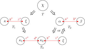
Figure 6. Diamond diagram proving local confluence in the case $A\subsetneq Y$.

The cases $A\subsetneq Z$, $B\subsetneq Y$, $B\subsetneq Z$ are similar to the case $A\subsetneq Y$, so from now on we can assume that $A\cap Y$, $A\cap Z$, $B\cap Y$, $B\cap Z$ are all nonempty. Lemma 3.9 then implies that each of $A\cap Y$, $A\cap Z$, $B\cap Y$ and $B\cap Z$ is a nontrivial module of $\chi$. We use this to further decompose $T_{1}$ and $T_{2}$ in ways that eventually reduce to the same term. The specific decomposition depends on which of $A\cap Y$, $A\cap Z$, $B\cap Y$, $B\cap Z$ contain non-extremal elements. We spell out two representative cases and leave the remaining, routine, check to the reader.

Case 1: each of $A\cap Y$, $A\cap Z$, $B\cap Y$, $B\cap Z$ contains at least one non-extremal element.

Many different chirotopes now enter the stage, so we record their ground sets and proxies in tables to help the reader keep track of them.

The ground set of $\kappa$ is $Y\cup\{y^{*}\}=(A\cap Y)\cup(B\cap Y)\cup\{y^{*}\}$ and $\chi$ and $\kappa$ coincide on $Y$. It follows that $A\cap Y$ and $B\cap Y$ are disjoint nontrivial modules of $\kappa$, and $\kappa$ therefore decomposes into $\kappa=\sigma\mathchoice{\sideset{{}_{s^{*}}}{{}_{x_{AY}}}{\operatorname{\textup{\Bowtie}}}}{\sideset{{}_{s^{*}}}{{}_{x_{AY}}}{\operatorname{\textup{\Bowtie}}}}{\sideset{{}_{s^{*}}}{{}_{x_{AY}}}{\scriptstyle\operatorname{\textup{\Bowtie}}}}{\sideset{{}_{s^{*}}}{{}_{x_{AY}}}{\scriptstyle\operatorname{\textup{\Bowtie}}}}\kappa^{\triangle}\mathchoice{\sideset{{}_{x_{BY}}}{{}_{p^{*}}}{\operatorname{\textup{\Bowtie}}}}{\sideset{{}_{x_{BY}}}{{}_{p^{*}}}{\operatorname{\textup{\Bowtie}}}}{\sideset{{}_{x_{BY}}}{{}_{p^{*}}}{\scriptstyle\operatorname{\textup{\Bowtie}}}}{\sideset{{}_{x_{BY}}}{{}_{p^{*}}}{\scriptstyle\operatorname{\textup{\Bowtie}}}}\pi$.

Chirotope	Ground set	Proxies
$\kappa$	$Y\cup\{y^{*}\}$	$y^{*}$
$\sigma$	$(A\cap Y)\cup\{s^{*}\}$	$s^{*}$
$\pi$	$(B\cap Y)\cup\{p^{*}\}$	$p^{*}$
$\kappa^{\triangle}$	$\{x_{AY},x_{BY},y^{*}\}$	$x_{AY},x_{BY},y^{*}$

Chirotope	Ground set	Proxies
$\xi$	$Z\cup\{z^{*}\}$	$z^{*}$
$\tau$	$(B\cap Z)\cup\{t^{*}\}$	$t^{*}$
$\rho$	$(A\cap Z)\cup\{r^{*}\}$	$r^{*}$
$\xi^{\triangle}$	$\{x_{AZ},x_{BZ},z^{*}\}$	$x_{AZ},x_{BZ},z^{*}$

Similarly, the ground set of $\xi$ is $Z\cup\{z^{*}\}=(A\cap Z)\cup(B\cap Z)\cup\{z^{*}\}$ and $\chi$ and $\xi$ coincide on $Z$. It follows that $A\cap Z$ and $B\cap Z$ are disjoint nontrivial modules of $\xi$, and $\xi$ therefore decomposes into $\xi=\tau\mathchoice{\sideset{{}_{t^{*}}}{{}_{x_{BZ}}}{\operatorname{\textup{\Bowtie}}}}{\sideset{{}_{t^{*}}}{{}_{x_{BZ}}}{\operatorname{\textup{\Bowtie}}}}{\sideset{{}_{t^{*}}}{{}_{x_{BZ}}}{\scriptstyle\operatorname{\textup{\Bowtie}}}}{\sideset{{}_{t^{*}}}{{}_{x_{BZ}}}{\scriptstyle\operatorname{\textup{\Bowtie}}}}\xi^{\triangle}\mathchoice{\sideset{{}_{x_{AZ}}}{{}_{r^{*}}}{\operatorname{\textup{\Bowtie}}}}{\sideset{{}_{x_{AZ}}}{{}_{r^{*}}}{\operatorname{\textup{\Bowtie}}}}{\sideset{{}_{x_{AZ}}}{{}_{r^{*}}}{\scriptstyle\operatorname{\textup{\Bowtie}}}}{\sideset{{}_{x_{AZ}}}{{}_{r^{*}}}{\scriptstyle\operatorname{\textup{\Bowtie}}}}\rho$.

Altogether, we can transform $T_{1}$ into

$$T_{1}\quad=\qquad\leavevmode\hbox to55.68pt{\vbox to18.69pt{\text{[drawing]}}}\qquad\xrightarrow{\operatorname{\textup{\Bowtie}}}^{*}\qquad\leavevmode\hbox to102.76pt{\vbox to65.77pt{\text{[drawing]}}}\qquad\xrightarrow{\lozenge}\qquad\leavevmode\hbox to65.77pt{\vbox to65.77pt{\text{[drawing]}}} \kappa \xi \bullet \bullet y^{*} z^{*} \kappa^{\triangle} \xi^{\triangle} \sigma \pi \rho \tau \bullet \bullet \bullet \bullet \bullet \bullet \bullet \bullet \bullet \bullet y^{*} z^{*} p^{*} t^{*} r^{*} s^{*} x_{AY} x_{AZ} x_{BZ} x_{BY} \chi^{\square} \sigma \pi \rho \tau \bullet \bullet \bullet \bullet \bullet \bullet \bullet \bullet p^{*} t^{*} r^{*} s^{*} x_{AY} x_{AZ} x_{BZ} x_{BY} \kappa \xi \bullet \bullet y^{*} z^{*} \kappa^{\triangle} \xi^{\triangle} \sigma \pi \rho \tau \bullet \bullet \bullet \bullet \bullet \bullet \bullet \bullet \bullet \bullet y^{*} z^{*} p^{*} t^{*} r^{*} s^{*} x_{AY} x_{AZ} x_{BZ} x_{BY} \chi^{\square} \sigma \pi \rho \tau \bullet \bullet \bullet \bullet \bullet \bullet \bullet \bullet p^{*} t^{*} r^{*} s^{*} x_{AY} x_{AZ} x_{BZ} x_{BY}$$

where the last transformation is a contraction of the central edge between the two convex chirotopes $\kappa^{\Delta}$ and $\xi^{\Delta}$; the resulting node is decorated with a convex chirotopes on four elements, all proxies; we denote this chirotope by $\chi^{\square}$, and its proxy elements are $x_{AY},x_{AZ},x_{BZ},x_{BY}$. Similarly, we have

$$T_{2}\quad=\qquad\leavevmode\hbox to55.68pt{\vbox to18.69pt{\text{[drawing]}}}\quad\xrightarrow{\operatorname{\textup{\Bowtie}}}^{*}\quad\leavevmode\hbox to102.76pt{\vbox to65.77pt{\text{[drawing]}}}\qquad\xrightarrow{\lozenge}\qquad\leavevmode\hbox to65.77pt{\vbox to65.77pt{\text{[drawing]}}}, \alpha \beta \bullet \bullet a^{*} b^{*} \alpha^{\triangle} \beta^{\triangle} \rho \sigma \tau \pi \bullet \bullet \bullet \bullet \bullet \bullet \bullet \bullet \bullet \bullet a^{*} b^{*} t^{*} p^{*} s^{*} r^{*} x_{AZ} x_{AY} x_{BY} x_{BZ} \chi^{\square} \rho \sigma \tau \pi \bullet \bullet \bullet \bullet \bullet \bullet \bullet \bullet s^{*} p^{*} t^{*} r^{*} x_{AZ} x_{BZ} x_{BY} x_{AY} \alpha \beta \bullet \bullet a^{*} b^{*} \alpha^{\triangle} \beta^{\triangle} \rho \sigma \tau \pi \bullet \bullet \bullet \bullet \bullet \bullet \bullet \bullet \bullet \bullet a^{*} b^{*} t^{*} p^{*} s^{*} r^{*} x_{AZ} x_{AY} x_{BY} x_{BZ} \chi^{\square} \rho \sigma \tau \pi \bullet \bullet \bullet \bullet \bullet \bullet \bullet \bullet s^{*} p^{*} t^{*} r^{*} x_{AZ} x_{BZ} x_{BY} x_{AY}$$

with the same chirotope $\chi^{\square}$ as before, and all other appearing chirotopes recalled or defined in the tables below.

Chirotope	Ground set	Proxies
$\alpha$	$A\cup\{a^{*}\}$	$a^{*}$
$\sigma$	$(A\cap Y)\cup\{s^{*}\}$	$s^{*}$
$\rho$	$(A\cap Z)\cup\{r^{*}\}$	$r^{*}$
$\alpha^{\triangle}$	$\{x_{AY},x_{AZ},a^{*}\}$	$x_{AY},x_{AZ},a^{*}$

Chirotope	Ground set	Proxies
$\beta$	$B\cup\{b^{*}\}$	$b^{*}$
$\pi$	$(B\cap Y)\cup\{p^{*}\}$	$p^{*}$
$\tau$	$(B\cap Z)\cup\{t^{*}\}$	$t^{*}$
$\beta^{\triangle}$	$\{x_{BY},x_{BZ},b^{*}\}$	$x_{BY},x_{BZ},b^{*}$

We stress that the chirotopes $\sigma,\rho,\tau,\pi$ and $\chi^{\square}$ are the same in both decompositions, as they are restriction of our initial chirotope $\chi$ to the same sets (replacing proxy elements by arbitrary elements in the sets that they represent). The two trees obtained at the far right of both derivations are identical. Since each of $A\cap Y$, $A\cap Z$, $B\cap Y$ and $B\cap Z$ contains a non-extremal point, the chirotopes $\sigma,\rho,\tau$ and $\pi$ are non convex, and all transformations in the decompositions of $T_{1}$ and $T_{2}$ given above are valid rules for $\Rightarrow$, and the statement follows.

Case 2: each of $A\cap Z$, $B\cap Y$, $B\cap Z$ contains a non-extremal element, but $A\cap Y$ does not.

We now define $\kappa^{\pentago}\stackrel{{\scriptstyle\text{def}}}{{=}}\sigma\mathchoice{\sideset{{}_{s^{*}}}{{}_{x_{AY}}}{\operatorname{\textup{\Bowtie}}}}{\sideset{{}_{s^{*}}}{{}_{x_{AY}}}{\operatorname{\textup{\Bowtie}}}}{\sideset{{}_{s^{*}}}{{}_{x_{AY}}}{\scriptstyle\operatorname{\textup{\Bowtie}}}}{\sideset{{}_{s^{*}}}{{}_{x_{AY}}}{\scriptstyle\operatorname{\textup{\Bowtie}}}}\kappa^{\triangle}$ and $\alpha^{\pentago}\stackrel{{\scriptstyle\text{def}}}{{=}}\sigma\mathchoice{\sideset{{}_{s^{*}}}{{}_{x_{AY}}}{\operatorname{\textup{\Bowtie}}}}{\sideset{{}_{s^{*}}}{{}_{x_{AY}}}{\operatorname{\textup{\Bowtie}}}}{\sideset{{}_{s^{*}}}{{}_{x_{AY}}}{\scriptstyle\operatorname{\textup{\Bowtie}}}}{\sideset{{}_{s^{*}}}{{}_{x_{AY}}}{\scriptstyle\operatorname{\textup{\Bowtie}}}}\alpha^{\triangle}$. We note that $\kappa^{\pentago}\mathchoice{\sideset{{}_{y^{*}}}{{}_{z^{*}}}{\operatorname{\textup{\Bowtie}}}}{\sideset{{}_{y^{*}}}{{}_{z^{*}}}{\operatorname{\textup{\Bowtie}}}}{\sideset{{}_{y^{*}}}{{}_{z^{*}}}{\scriptstyle\operatorname{\textup{\Bowtie}}}}{\sideset{{}_{y^{*}}}{{}_{z^{*}}}{\scriptstyle\operatorname{\textup{\Bowtie}}}}\xi^{\triangle}=\alpha^{\pentago}\mathchoice{\sideset{{}_{a^{*}}}{{}_{b^{*}}}{\operatorname{\textup{\Bowtie}}}}{\sideset{{}_{a^{*}}}{{}_{b^{*}}}{\operatorname{\textup{\Bowtie}}}}{\sideset{{}_{a^{*}}}{{}_{b^{*}}}{\scriptstyle\operatorname{\textup{\Bowtie}}}}{\sideset{{}_{a^{*}}}{{}_{b^{*}}}{\scriptstyle\operatorname{\textup{\Bowtie}}}}\beta^{\triangle}$, since both are restrictions of $\chi$ on $(A\cap Y)\cup\{x_{AZ},x_{BZ},x_{BY}\}$ (replacing proxy elements by arbitrary elements in the sets that they represent). We denote this chirotope by $\chi^{\hexago}$. All of $\alpha^{\pentago}$, $\kappa^{\pentago}$ and $\chi^{\hexago}$ are convex. Then we can write

$$T_{1} =\ \leavevmode\hbox to55.68pt{\vbox to18.69pt{\text{[drawing]}}}\quad\xrightarrow{\operatorname{\textup{\Bowtie}}}^{*}\quad\leavevmode\hbox to102.76pt{\vbox to65.77pt{\text{[drawing]}}}\quad\xrightarrow{\lozenge}\quad\leavevmode\hbox to65.77pt{\vbox to65.77pt{\text{[drawing]}}}; \kappa \xi \bullet \bullet y^{*} z^{*} \kappa^{\pentago} \xi^{\triangle} \pi \rho \tau \bullet \bullet \bullet \bullet \bullet \bullet \bullet \bullet y^{*} z^{*} p^{*} t^{*} r^{*} x_{AZ} x_{BZ} x_{BY} \chi^{\hexago} \pi \rho \tau \bullet \bullet \bullet \bullet \bullet \bullet p^{*} t^{*} r^{*} x_{AZ} x_{BZ} x_{BY} \kappa \xi \bullet \bullet y^{*} z^{*} \kappa^{\pentago} \xi^{\triangle} \pi \rho \tau \bullet \bullet \bullet \bullet \bullet \bullet \bullet \bullet y^{*} z^{*} p^{*} t^{*} r^{*} x_{AZ} x_{BZ} x_{BY} \chi^{\hexago} \pi \rho \tau \bullet \bullet \bullet \bullet \bullet \bullet p^{*} t^{*} r^{*} x_{AZ} x_{BZ} x_{BY}$$

$$T_{2} =\ \leavevmode\hbox to55.68pt{\vbox to18.69pt{\text{[drawing]}}}\quad\xrightarrow{\operatorname{\textup{\Bowtie}}}^{*}\quad\leavevmode\hbox to102.76pt{\vbox to65.77pt{\text{[drawing]}}}\quad\xrightarrow{\lozenge}\quad\leavevmode\hbox to65.77pt{\vbox to65.77pt{\text{[drawing]}}}, \alpha \beta \bullet \bullet a^{*} b^{*} \alpha^{\pentago} \beta^{\triangle} \rho \tau \pi \bullet \bullet \bullet \bullet \bullet \bullet \bullet \bullet a^{*} b^{*} t^{*} p^{*} r^{*} x_{AZ} x_{BY} x_{BZ} \chi^{\hexago} \rho \tau \pi \bullet \bullet \bullet \bullet \bullet \bullet p^{*} t^{*} r^{*} x_{AZ} x_{BZ} x_{BY} \alpha \beta \bullet \bullet a^{*} b^{*} \alpha^{\pentago} \beta^{\triangle} \rho \tau \pi \bullet \bullet \bullet \bullet \bullet \bullet \bullet \bullet a^{*} b^{*} t^{*} p^{*} r^{*} x_{AZ} x_{BY} x_{BZ} \chi^{\hexago} \rho \tau \pi \bullet \bullet \bullet \bullet \bullet \bullet p^{*} t^{*} r^{*} x_{AZ} x_{BZ} x_{BY}$$

showing the local confluence in this case. Other cases are treated similarly. ∎

4.3.5. Concluding the proof of Theorem 1.3

We can now put things together to prove existence and uniqueness of the canonical chirotope tree representing any given chirotope $\chi$.

Let $\chi$ be a chirotope. As noticed in Section 4.3.2, the existence of a canonical chirotope tree representing $\chi$ is a consequence of Lemma 4.9. Moreover, by Lemma 4.10 any canonical chirotope tree representing $\chi$ can be obtained from $T^{tr}_{\chi}$ through the rewriting rule $\Rightarrow$. We also observe that we can never apply any further rewriting $\Rightarrow$ to a canonical chirotope tree, i.e. these are terminal states. But we have proved the confluence of the rewriting rule $\Rightarrow$ (Proposition 4.11, combined with Newman’s lemma), so that for a given initial state, there is a unique possible terminal state. Consequenly, there is a unique canonical chirotope tree representing $\chi$, and Theorem 1.3 is proved. ∎

5. Almost all realizable chirotopes are indecomposable

In this section, we consider only realizable chirotopes. Recall from the introduction that $t_{n}$ and $d_{n}$ are respectively the number of realizable chirotopes and decomposable realizable chirotopes on $\{1,\dots,n\}$. Our goal is to prove Theorem 1.5, which we copy here for convenience.

Theorem 1.5. For large $n$, we have $3\left(n-\mathcal{O}(n^{-2})\right)t_{n-1}\leq d_{n}\leq\mathcal{O}(n^{-3})t_{n}$.

Stated differently, a uniform random realizable chirotope $\chi_{n}$ on $\{1,\dots,n\}$, is indecomposable with probability $1-\mathcal{O}(n^{-3})$.

5.1. A consequence for unlabeled chirotopes

Before proving the theorem, let us state a consequence for unlabeled chirotopes. By definition, an unlabeled chirotopes is an equivalence class of chirotopes for the following relation: $\chi:(X)_{3}\to\{\pm 1\}$ and $\chi^{\prime}:(Y)_{3}\to\{\pm 1\}$ are equivalent if there exists a bijection $\phi:X\to Y$ such that, for all $x_{1},x_{2},x_{3}$ in $X$

$$\chi^{\prime}(\phi(x_{1}),\phi(x_{2}),\phi(x_{3}))=\chi(x_{1},x_{2},x_{3}).$$

Many natural notions and properties of chirotopes (being realizable, the number of extreme points, etc.) do not depend on its labeling and are thus well-defined on unlabeled chirotopes. The notion of indecomposability is such a notion.

We remark that, to an unlabeled chirotope correspond several chirotopes on $\{1,\cdots,n\}$, the number of which can vary depending on its automorphism group. This implies that taking a uniform random realizable chirotope on $\{1,\dots,n\}$ forgetting its labeling or taking directly a uniform random unlabeled realizable chirotope on $n$ elements lead to two different probability distributions. However, symmetry can be controlled, and Theorem 1.5 implies the following.

Corollary 5.1.

Let $\bar{\chi}_{n}$ be a uniform random unlabeled realizable chirotope on $n$ elements. Then, $\bar{\chi}_{n}$ is indecomposable with probability $1-\mathcal{O}(n^{-2})$.

Proof.

Let $t^{u}_{n}$ denote the number of unlabeled realizable chirotopes on $n$ elements and $d^{u}_{n}$ the number of decomposable ones. Since a chirotope on $n$ elements has at most $n$ symmetries [GW23, Theorem 1.5], we have

$$\frac{t_{n}}{n!}\leq t_{n}^{u}\leq\frac{t_{n}}{(n-1)!}\qquad\text{and}\qquad\frac{d_{n}}{n!}\leq d_{n}^{u}\leq\frac{d_{n}}{(n-1)!}.$$

Theorem 1.5 asserts that $d_{n}/t_{n}=\mathcal{O}(n^{-3})$, from which we get

$$\frac{d_{n}^{u}}{t_{n}^{u}}\leq n\frac{d_{n}}{t_{n}}=\mathcal{O}(n^{-2}).\qed$$

5.2. Some classical estimates on the number of realizable chirotopes

We start by recalling essentially known results about the number $t_{n}$ of realizable chirotopes on $\{1,\dots,n\}$. A general reference on this topic is [GP93, Section 6]. The first statement that we need is the following non-asymptotic version of the case $d=2$ in [GP93, Theorem 6.6].

Proposition 5.2.

For all $n\geq 2$, we have $t_{n}\leq e^{2n}(n-1)^{4n}$.

Proof.

We copy here essentially the argument given in [GP93]. Let $\mathfrak{p}_{i}=(p_{i,x},p_{i,y})$, for $1\leq i\leq n$, represent an unknown set of $n$ points in $\mathbb{R}^{2}$, indexed by $\{1,\dots,n\}$. As already noticed in the proof of Lemma 2.4, for $i<j<k$ in $\{1,\dots,n\}$, we have

$$\chi(\mathfrak{p}_{i},\mathfrak{p}_{j},\mathfrak{p}_{k})=\operatorname{sgn}\left[\det\left(\begin{array}[]{ccc}p_{i,x}&p_{j,x}&p_{k,x}\\ p_{i,y}&p_{j,y}&p_{k,y}\\ 1&1&1\end{array}\right)\right].$$

The determinant in the right-hand side is a polynomial of degree $2$ in the variables $\{p_{i,x},p_{i,y},1\leq i\leq n\}$, which we denote $D_{i,j,k}$. A realizable chirotope on $\{1,\dots,n\}$ corresponds to a sign pattern of the collection $(D_{i,j,k})_{i<j<k}$ of polynomials, i.e. a choice of a sign for each $D_{i,j,k}$ which can be realized by some real specialization of the variables $\{p_{i,x},p_{i,y},1\leq i\leq n\}$. From a result of Warren [War68], the number of such sign patterns for general collection of polynomials is bounded by $(\tfrac{4edm}{N})^{N}$, where $d$ is the degree of the polynomials, $m$ their number and $N$ the number of variables. In our case $d=2$, $m=\binom{n}{3}$ and $N=2n$, and we get

$$t_{n}\leq\left(4e\frac{2\binom{n}{3}}{2n}\right)^{2n}$$

The lemma follows using the simple bound $\binom{n}{3}\leq n(n-1)^{2}/6$. ∎

The following lemma is implicit in the discussion preceeding Theorem 6.1 in [GP93].

Lemma 5.3.

There exists a universal constant $K$ in $(0,1/8]$ such that, for all $n\geq 3$, we have $t_{n+1}\geq K\,n^{4}\,t_{n}$.

Sketch of proof.

The number $t_{n+1}$ rewrites as the sum, over all realizable chirotopes $\chi$ on $[n]$, of the number of extensions of $\chi$, meaning the number of realizable chirotopes on $[n+1]$ whose restriction to (triples of) $[n]$ is $\chi$. Fix a geometric realization $P$ of $\chi$; the number of extensions of $\chi$ is bounded from below by the number of chirotopes realized by $1$-point extensions of $P$. This is exactly the number of cells in the arrangement of the $\binom{n}{2}$ lines through pairs of points of $P$, which is [Zas97, p. 65]

$$\binom{\binom{n}{2}}{2}+\binom{n}{2}+1-n\binom{n-2}{2}=\frac{n^{4}}{8}-\frac{r(n)}{8},$$

with $r(n)=6n^{3}-23n^{2}+26n-8\leq\frac{n^{4}}{2}$ for $n\geq 3$, by a simple function analysis. The statement follows from this bound by taking $K=\frac{1}{16}$. ∎

5.3. Some basic relations between numbers of chirotopes

Let $t^{*}_{n}$ as the number of realizable chirotopes on $\{1,\dots,n\}$, in which $n$ is an extreme element. We now relate $d_{n}$, $t_{n}$ and $t_{n}^{*}$, starting with the last two.

Lemma 5.4.

For each $n\geq 3$, we have $\frac{3}{n}t_{n}\leq t_{n}^{*}\leq\frac{4}{n}t_{n}$.

Proof.

For a chirotope $\chi$, we denote by $\mathrm{ext}(\chi)$ its number of extreme elements. By symmetry, we have:

$$\sum_{\chi\in{\mathcal{X}}_{n}}\mathrm{ext}(\chi)=\big{|}\{(\chi,i)\in{\mathcal{X}}_{n}\times[n]\colon i\text{ is extreme in }\chi\}\big{|}=nt_{n}^{*}.$$

Hence,

$$\frac{t_{n}^{*}}{t_{n}}=\frac{1}{nt_{n}}\sum_{\chi\in{\mathcal{X}}_{n}}\mathrm{ext}(\chi)=\frac{1}{n}\mathbb{E}[\mathrm{ext}(\chi)],$$

where $\chi$ is chosen uniformly at random in $\mathcal{X}_{n}$. By [GW23, Theorem 1.2],

$$\mathbb{E}[\mathrm{ext}(\chi)]=4-\frac{8}{n^{2}-n+2},$$

which is between $3$ and $4$. ∎

Now, let us turn our attention to $d_{n}$.

Lemma 5.5.

For each $n\geq 5$, we have

(16) $$3n(t_{n-1}-d_{n-1})\leq d_{n}\leq\sum_{n_{1}+n_{2}=n\atop n_{1},n_{2}\geq 2}\binom{n}{n_{1}}\,t^{*}_{n_{1}+1}\,t^{*}_{n_{2}+1}.$$

Proof.

Let $\mathcal{X}^{*}_{n}$ denote the set of realizable chirotopes on $[n]\stackrel{{\scriptstyle\text{def}}}{{=}}\{1,2,\dots,n\}$ such that $n$ is extreme, and $\mathcal{D}_{n}$ the set of decomposable realizable chirotopes of size $n$. We define an application $\phi$ that associates to a pair $(\chi,M)$ – where $\chi\in\mathcal{D}_{n}$ and $M\subseteq[n]$ is a nontrivial module of $\chi$ – a tuple $\phi(\chi,M)=(\chi_{1},\chi_{2},M)$ constructed as follows. Letting $n_{1}\stackrel{{\scriptstyle\text{def}}}{{=}}|M|$ and $n_{2}\stackrel{{\scriptstyle\text{def}}}{{=}}n-n_{1}$,

• $\chi_{1}$ is the chirotope obtained by replacing the elements of $[n]\setminus M$ by a single element labeled $n_{1}+1$, and relabeling $M$ from $1$ to $n_{1}$ consistently with the order of $M$;

• $\chi_{2}$ is the chirotope obtained, similarly, by replacing the elements of $M$ by a single element labeled $n_{2}+1$, and relabeling $[n]\setminus M$ from $1$ to $n_{2}$ consistently.

From Propositions 3.2 and 3.6, it holds that $n_{1}+1$ and $n_{2}+1$ are extreme elements in $\chi_{1}$ and $\chi_{2}$ respectively, i.e.  $\chi_{1}\in\mathcal{X}^{*}_{n_{1}+1}$ and $\chi_{2}\in\mathcal{X}^{*}_{n_{2}+1}$. We claim that $\phi$ is bijective. Indeed, take a triple $(\chi_{1},\chi_{2},M)$, with $\chi_{1}\in\mathcal{X}^{*}_{n_{1}+1}$, $\chi_{2}\in\mathcal{X}^{*}_{n_{2}+1}$ and $M\subseteq[n]$. Let us define $\chi_{1}^{M}$ as the chirotope over $M\cup\{x^{*}\}$ obtained by renaming, in $\chi_{1}$, the (extreme) element $n_{1}+1$ as $x^{*}$ and $[n_{1}]$ as $M$, increasingly. The chirotope $\chi_{2}^{[n]\setminus M}$ is defined similarly with label set $([n]\setminus M)\cup\{y^{*}\}$. Finally, we set $\chi=\chi_{1}^{M}\mathchoice{\sideset{{}_{x^{*}}}{{}_{y^{*}}}{\operatorname{\textup{\Bowtie}}}}{\sideset{{}_{x^{*}}}{{}_{y^{*}}}{\operatorname{\textup{\Bowtie}}}}{\sideset{{}_{x^{*}}}{{}_{y^{*}}}{\scriptstyle\operatorname{\textup{\Bowtie}}}}{\sideset{{}_{x^{*}}}{{}_{y^{*}}}{\scriptstyle\operatorname{\textup{\Bowtie}}}}\chi_{2}^{[n]\setminus M}$ and define $\Psi(\chi_{1},\chi_{2},M)=(\chi,M)$. One readily checks that $\phi$ and $\Psi$ are inverse of each other, showing that $\phi$ is bijective.

As a consequence, we have

$$d_{n}\leq|\{(\chi,M)\,:\,\chi\in\mathcal{D}_{n},\,M\text{ nontrivial module of }\chi\}|=\sum_{n_{1}+n_{2}=n\atop n_{1},n_{2}\geq 2}\binom{n}{n_{1}}\,t^{*}_{n_{1}+1}\,t^{*}_{n_{2}+1},$$

proving the upper bound in Eq. 16.

On the other hand, the chirotopes $\chi_{1}\mathchoice{\sideset{{}_{x^{*}}}{{}_{y^{*}}}{\operatorname{\textup{\Bowtie}}}}{\sideset{{}_{x^{*}}}{{}_{y^{*}}}{\operatorname{\textup{\Bowtie}}}}{\sideset{{}_{x^{*}}}{{}_{y^{*}}}{\scriptstyle\operatorname{\textup{\Bowtie}}}}{\sideset{{}_{x^{*}}}{{}_{y^{*}}}{\scriptstyle\operatorname{\textup{\Bowtie}}}}\chi_{2}$ are different for any $\chi_{1}\in{\cal X}_{3}$ and $\chi_{2}\in{\cal X}_{n-1}\setminus{\cal D}_{n-1}$ (this can easily be seen e.g. via Theorem 1.3). Since there are $2$ chirotopes on $\{1,2,3\}$, it follows that $d_{n}\geq 2\binom{n}{2}i^{*}_{n-1}$ where $i^{*}_{n-1}$ is the number of indecomposable realizable chirotopes on $[n-1]$ in which $n-1$ is an extreme point. Using the same argument as in Lemma 5.4, we have

$$i^{*}_{n-1}\geq\frac{3}{n-1}(t_{n-1}-d_{n-1}),$$

concluding the proof of the lower bound in Eq. 16. ∎

Combining Lemmas 5.4 and 5.5, we get

(17) $$d_{n}\leq 16\sum_{n_{1}+n_{2}=n\atop n_{1},n_{2}\geq 2}\binom{n}{n_{1}}\,\frac{t_{n_{1}+1}\,t_{n_{2}+1}}{(n_{1}+1)\,(n_{2}+1)}.$$

5.4. Bounding the sum

The goal is to prove that the upper bound in Eq. 17 behaves as $\mathcal{O}(n^{-3}t_{n})$. We fix some $\varepsilon$ in $(0,1/2)$ independent of $n$ and split the sum into two parts.

(18) $$d^{\rm small}_{n} =\sum_{\begin{subarray}{c}n_{1}+n_{2}=n\\ 2\leq\min(n_{1},n_{2})< \varepsilon n\end{subarray}}\binom{n}{n_{1}}\,\frac{t_{n_{1}+1}\,t_{n_{2}+1}}{(n_{1}+1)\,(n_{2}+1)},\text{ and }$$

(19) $$d^{\rm large}_{n} =\sum_{\begin{subarray}{c}n_{1}+n_{2}=n\\ \varepsilon n\leq n_{1},n_{2}\leq (1-\varepsilon)n\end{subarray}}\binom{n}{n_{1}}\,\frac{t_{n_{1}+1}\,t_{n_{2}+1}}{(n_{1}+1)\,(n_{2}+1)}.$$

The part $d^{\rm small}_{n}$ can be bounded using the classical estimates on the number of realizable chirotopes given in Section 5.2.

Lemma 5.6.

For $\varepsilon$ small enough, we have $\frac{d^{\rm small}_{n}}{t_{n}}=\mathcal{O}(n^{-3})$ as $n$ tends to $+\infty$.

Proof.

Assuming $\varepsilon<\tfrac{1}{2}$, we write

$$n^{3}\frac{d^{\rm small}_{n}}{t_{n}} =2n^{3}\sum_{n_{1}+n_{2}=n\atop 2\leq n_{1}<\varepsilon n}\binom{n}{n_{1}}\,\frac{t_{n_{1}+1}}{n_{1}+1}\,\frac{t_{n_{2}+1}}{(n_{2}+1)t_{n}}.$$

Iterating Lemma 5.3, we get

$$\frac{t_{n_{2}+1}}{t_{n}}\leq\frac{1}{K^{n_{1}-1}(n_{2}+1)^{4}\ldots(n-1)^{4}}.$$

On the other hand, Proposition 5.2 yields:

$$\frac{t_{n_{1}+1}}{n_{1}+1}\leq e^{2n_{1}+2}n_{1}^{4(n_{1}+1)-1}.$$

Bringing everything together gives us:

$$n^{3}\frac{d^{\rm small}_{n}}{t_{n}} \leq 2\sum_{n_{1}+n_{2}=n\atop 2\leq n_{1}\leq\varepsilon n}\frac{n^{4}(n-1)\ldots(n_{2}+1)}{n_{1}!}\frac{e^{2n_{1}+2}n_{1}^{4(n_{1}+1)-1}}{K^{n_{1}-1}(n_{2}+1)^{5}(n_{2}+2)^{4}\ldots(n-1)^{4}}$$

Using that for $n$ large enough, $n^{4}\leq 2(n-2)(n-1)^{3}$, and $n_{1}!\geq\left(\frac{n_{1}}{e}\right)^{n_{1}}$, we get

$$n^{3}\frac{d^{\rm small}_{n}}{t_{n}} \leq 4Ke^{2}\sum_{n_{1}+n_{2}=n\atop 2\leq n_{1}\leq\varepsilon n}\left(\frac{e}{n_{1}}\right)^{n_{1}}\frac{e^{2n_{1}}n_{1}^{4(n_{1}+1)-1}}{K^{n_{1}}(n_{2}+1)^{4}(n_{2}+2)^{3}\ldots(n-3)^{3}(n-2)^{2}}\,.$$

When $n_{2}=n-2$, the product in the denominator $(n_{2}+1)^{4}(n_{2}+2)^{3}\ldots(n-3)^{3}(n-2)^{2}$ should be interpreted as $1$ (in this case, we use $n^{4}\leq 2(n-1)^{4}$).

Each of the $3(n-n_{2}-2)=3n_{1}-6$ polynomial factors in the denominator are bounded from below by

$$n_{2}\geq(1-\varepsilon)n\geq\frac{1-\varepsilon}{\varepsilon}n_{1}\,.$$

Hence, we get, for $n$ large enough,

$$n^{3}\frac{d^{\rm small}_{n}}{t_{n}} \leq 4Ke^{2}\left(\frac{1-\varepsilon}{\varepsilon}\right)^{6}\sum_{2\leq n_{1}\leq\varepsilon n}\left(\frac{e^{3}}{K}\left(\frac{\varepsilon}{1-\varepsilon}\right)^{3}\right)^{n_{1}}\frac{n_{1}^{4(n_{1}+1)-1}}{n_{1}^{n_{1}}n_{1}^{3n_{1}-6}}$$

$$\leq 4Ke^{2}\left(\frac{1-\varepsilon}{\varepsilon}\right)^{6}\sum_{n_{1}\geq 2}\left(\frac{e^{3}}{K}\left(\frac{\varepsilon}{1-\varepsilon}\right)^{3}\right)^{n_{1}}n_{1}^{9}.$$

For $\varepsilon$ small enough, we have a convergent series, showing that the right-hand size is bounded by a finite constant. ∎

We note that the above strategy (via Lemmas 5.3 and 5.2) would even fail to show that $t_{n/2+1}^{2}\leq t_{n}$, and can therefore not be used to control $d^{\rm large}_{n}$. In the next section, we will prove the following lemma with a completely different method.

Lemma 5.7.

For $n\geq\frac{3}{\varepsilon}$, we have $\displaystyle t_{n}\geq\frac{3K\varepsilon^{7}}{4}\,n^{3}\,d^{\rm large}_{n}$, where $K$ is the constant introduced in Lemma 5.3.

Proof of Theorem 1.5.

Combining Eqs. 17, 18, 19, 5.6 and 5.7, we find that $\frac{d_{n}}{t_{n}}=\mathcal{O}(n^{-3})$, showing the upper bound in Theorem 1.5. The lower bound follows from Lemma 5.5, using that $\frac{d_{n-1}}{t_{n-1}}=\mathcal{O}(n^{-3})$. ∎

6. Quasi-modules and the proof of Lemma 5.7

Lemma 5.7 gives a lower bound on $t_{n}$ in terms of products $t_{n_{1}+1}t_{n_{2}+1}$ where $n_{1}+n_{2}=n$. We prove it by constructing, given two small realizable chirotopes, a larger one via a generalized substitution operation “along a segment” (defined in Section 6.2). This operation is not one-to-one, but the redundancy can be controlled using a notion of “quasi-modules” (defined in Section 6.1).

6.1. Quasi-modules

Let $\chi$ be a chirotope on a set $X$. Let $a,b\in X$ and let $Y$ be a subset of $X$ disjoint from $\{a,b\}$. The line $ab$ splits $Y$ into $Y=Y_{-1}\uplus Y_{1}$, where, for $i\in\{-1,1\}$,

$$Y_{i}=\{y\in Y,\,\chi(a,b,y)=i\}.$$

We call the set $\{Y_{-1},Y_{1}\}$ the bipartition of $Y$ induced by $a$ and $b$. Note that although switching $a$ and $b$ exchanges $Y_{-1}$ and $Y_{1}$, the induced bipartition is the same. A bipartition is called nontrivial if both $Y_{-1}$ and $Y_{1}$ are non-empty. This gives rise to a variant of the notion of modules.

Definition 6.1.

A subset $W$ of $X$ is called a quasi-module of a chirotope $\chi$ on $X$ if every pair $\{a,b\}$ of elements of $W$ defines the same bipartition of $X\setminus W$, and if this bipartition is nontrivial (meaning that neither part is empty).

We compare the above definition to our earlier definition of module (see Definition 3.5). If $M\subset X$ is a module of a chirotope $\chi$, then every pair of elements of $M$ defines the same bipartition on $X\setminus M$. However, this bipartition is trivial, so a module is not a quasi-module. Another difference is that the definition of module is symmetric in $M$ and $X\setminus M$, while that of quasi-module is not.

An example of quasi-module is given on Figure 7. On the other hand, consider a chirotope $\chi$ on $X$ with exactly three extreme elements $\{a,b,c\}$. Each of $\{a,b\}$, $\{a,c\}$ and $\{b,c\}$ defines the same bipartition $\{X\setminus\{a,b,c\},\emptyset\}$. Yet, the set $\{a,b,c\}$ is not a quasi-module as it fails the nontriviality condition.

Figure 7. Every line of two points in $W=\{a,b,c,d\}$ defines the same bipartition of points in $\{p,q,r\}$, so $W$ is a quasi-module. On the other hand, $\{a,b,c\}$ is not a quasi-module of that chirotope (because of element $d$).

It will be useful to control the number of quasi-modules of macroscopic size of any given chirotope.

Lemma 6.2.

For every $\varepsilon>0$ and for every $n\geq 1$ such that $\varepsilon n\geq 2$, every chirotope of size $n$ has at most $n^{2}/\varepsilon^{2}$ quasi-modules of size at least $\varepsilon\,n$.

Proof.

Fix a chirotope $\chi$ on a set $X$ of size $n$. We will use a double-counting argument based on an upper bound on the number of triples $(W,a,b)$, where $W$ is a quasi-module and $a\neq b$ are two points of $W$.

To construct such triples, we start by choosing two points $a\neq b$ in $X$. We label the elements of $X\setminus\{a,b\}$ as $x_{1}$, $x_{2}$, …, $x_{n-2}$ as follows. We start with the line $ab$ and rotate it in clockwise direction around $a$. The $i$-th point encountered gets the label $x_{i}$. Note that we rotate the whole line (infinite in both directions) and not only a half-line: for example, $x_{1}$ can be on either side of the line $ab$.

Figure 8. Turning the line $ab$ clockwise around $a$ reaches $\ell_{1},\ell_{2},\ell_{3}$ and $\ell_{4}$ in this order, yielding the labels $x_{1},x_{2},x_{3}$ and $x_{4}$.

Consider a quasi-module $W$ containing $\{a,b\}$. Assume that $W$ contains $x_{i}$ for some $i$. For any $j,k$ such that $j<i<k$, the lines $ab$ and $ax_{i}$ induce different bipartitions of $\{x_{j},x_{k}\}$, see Fig 9. This implies that either $x_{j}$ or $x_{k}$ is in $W$. Since this holds for any $j$ and $k$ such that $j<i<k$, any quasi-module $W$ containing $a,b$ is of the form

(20) $$W=\big{\{}a,b,x_{1},\cdots,x_{j},x_{k},\cdots,x_{n-2}\big{\}},$$

for some $0\leq j<k\leq n-1$. (The converse is not true in general, as our construction does not control the bipartitions of $X\setminus W$ induced by lines $bx_{s}$ or $x_{s}x_{t}$ for $x_{s}$, $x_{t}$ in $W$ (and $s\neq t$).) It follows that at most $\frac{1}{2}n^{2}$ quasi-modules $W$ contain two given points $a$ and $b$. There are thus at most $\frac{1}{2}n^{4}$ triples $(W,a,b)$ as above.

Figure 9. The lines $ab$ and $ax_{i}$ divide the plane into four quadrants. These lines induce the same bipartition of $\{x_{j},x_{k}\}$ if and only if these two points lie in equal or opposite quadrants. The labeling scheme of $X\setminus\{a,b\}$ ensures that this is not possible for any points on $\ell_{j}$ and $\ell_{k}$, respectively.

If we denote $w_{k}$ the number of quasi-modules of size $k$ of the chirotope $\chi$, then the number of triples $(W,a,b)$ as above is $\sum_{k=0}^{n}w_{k}k(k-1)$. Summing up, we have

$$\sum_{k\geq\varepsilon n}w_{k}\leq\frac{1}{\varepsilon n(\varepsilon n-1)}\sum_{k=0}^{n}w_{k}k(k-1)\leq\frac{1}{\varepsilon n(\varepsilon n-1)}\frac{n^{4}}{2}\leq\frac{n^{2}}{\varepsilon^{2}},$$

as announced. ∎

We conclude this section with the following lemma, which will be useful later.

Lemma 6.3.

Let $\chi$ be a chirotope on $X$ and $W$ be a quasi-module of $\chi$. There exists a unique pair $\{w_{1},w_{2}\}\subseteq W$ such that for all $a\in X\setminus W$ we have

(21) $$\forall w\in W\setminus\{w_{1},w_{2}\},\quad\chi(a,w_{1},w)=\chi(a,w,w_{2})\text{ and is independent of }w.$$

Proof.

The statement is trivial if $W$ has size two. Otherwise, fix an arbitrary point $b$ in $X\setminus W$. We claim that $b$ is extremal in the restriction of $\chi$ to $W\cup\{b\}$. Otherwise, by Lemma 2.1, $b$ would be contained in a triangle $w_{1}w_{2}w_{3}$ of points in $W$ i.e. one could find $w_{1},w_{2},w_{3}$ in $W$ such that

$$\chi(b,w_{1},w_{2})=\chi(b,w_{2},w_{3})=\chi(b,w_{3},w_{1})=1.$$

By the interiority axiom, this implies $\chi(w_{1},w_{2},w_{3})=1$. But from the definition of quasi-module, there must exist a point $c\in X\setminus W$ such that, for all $w,w^{\prime}$ in $W$, $\chi(b,w,w^{\prime})=\chi(c,w^{\prime},w)$. In particular,

$$\chi(c,w_{2},w_{1})=\chi(c,w_{3},w_{2})=\chi(c,w_{1},w_{3})=1.$$

Using again the interiority axiom, we get $\chi(w_{2},w_{1},w_{3})=1$, leading to a contradiction. Hence, $b$ is indeed extremal in the restriction of $\chi$ to $W\cup\{b\}$.

Therefore, by Lemma 2.2, the relation $w<_{b}w^{\prime}\Leftrightarrow\chi(b,w,w^{\prime})=1$ defines a strict total order on $W$. Call $w_{1}$ and $w_{2}$ the minimal and maximal elements of $W$ for this order relation. For all $w\in W\setminus\{w_{1},w_{2}\}$, we have $w_{1}<_{b}w<_{b}w_{2}$, i.e.

$$\chi(b,w_{1},w)=\chi(b,w,w_{2})=1.$$

In particular, Eq. 21 holds for $a=b$. It also for other elements $a\in X\setminus W$, using the fact that $W$ is a quasi-module. This proves the existence of the pair $(w_{1},w_{2})$.

The uniqueness also follows from the fact that $<_{b}$ is a total order. Only the pair constituted by the two extrema of this total order can satisfy Eq. 21 for $a=b$. ∎

We refer to the two elements $\{w_{1},w_{2}\}$ given by Lemma 6.3 as the antipodal elements of the quasi-module $W$.

6.2. Substituting a realizable chirotope along a segment

Let $\chi$ be a realizable chirotope on a set $X$ and let $a\in X$ be extreme for $\chi$. As we saw in Lemma 2.2, and immediately after, we can define $a_{+}$ (resp. $a_{-}$) as the unique element of $X$ such that $\chi(a,a_{+},x)=1$ for every $x\in X\setminus\{a,a_{+}\}$ (resp. such that $\chi(a_{-},a,x)=1$ for every $x\in X\setminus\{a,a_{-}\}$). (Geometrically, $a_{-}$, $a$ and $a_{+}$ are consecutive points on the convex hull of $\chi$.) We refer to $a_{+}$ (resp. $a_{-}$) as the successor (resp. the predecessor) of $a$ on the convex hull of $\chi$.

Definition 6.4.

Let $\chi$ be a realizable chirotope on a set $X$ and let $a$ be an element of $X$ extreme for $\chi$. Let $a_{+}$ and ${a_{-}}$ be, respectively, the successor and predecessor of $a$ on the convex hull of $\chi$. A $\delta$-squeezing of $(\chi,a)$ is a realization $\cal P$ of $\chi$ such that:

• $\mathfrak{p}_{a}=(0,1)$, $\mathfrak{p}_{a_{+}}=(-1,0)$ and $\mathfrak{p}_{a_{-}}=(1,0)$,

• the $y$-coordinates of every other point of $\cal P$ is at most $\delta$, and

• every line going through two points of $\cal P\setminus\{\mathfrak{p}_{a}\}$ has slope in $[-\delta,\delta]$.

Lemma 6.5.

Let $\chi$ be a realizable chirotope on a set $X$ and let $a$ be an element of $X$ extreme for $\chi$. For every $\delta>0$, the pair $(\chi,a)$ admits a $\delta$-squeezing.

Proof.

Let $\cal Q$ be a realization of $\chi$ in which $\mathfrak{q}_{a}$ is in an unbounded cell $\Sigma$ of the line arrangement $\big{\{}(\mathfrak{q}_{y},\mathfrak{q}_{z}),z,y\in X\setminus\{a\}\big{\}}$. (Such a realization exists by Lemma 2.4.) Applying a translation, a rotation and a scaling, we can further assume that $\mathfrak{q}_{a_{+}}=(-1,0)$ and $\mathfrak{q}_{a_{-}}=(1,0)$ while keeping $\mathfrak{q}_{a}$ in an unbounded cell $\Sigma$; note that $\mathfrak{q}_{a}$ (and thus $\Sigma$) lies above the $x$-axis. Let $\vec{u}=(u_{x},u_{y})$ be a direction such that $\mathfrak{q}_{a}+\mathbb{R}_{\geq 0}\vec{u}\subset\Sigma$. Note that $u_{y}$ can be chosen to be positive.

For any $\alpha\in\mathbb{R}$ and $\beta>0$, the transform $f_{\alpha,\beta}:(x,y)\mapsto(x+\alpha y,\beta y)$ preserves orientations and leaves the $x$-axis fixed. Moreover, for every point $(x_{0},y_{0})$ with $y_{0}>0$, there exists $\alpha\in\mathbb{R}$ such that $f_{\alpha,\frac{1}{y_{0}}}(x_{0},y_{0})=(0,1)$ (namely, $\alpha=-\tfrac{x_{0}}{y_{0}}$).

Now, let $t\in\mathbb{R}_{\geq 0}$ and consider the point $\mathfrak{p}(t)\stackrel{{\scriptstyle\text{def}}}{{=}}\mathfrak{q}_{a}+t\vec{u}$. Let $\alpha_{t}$ and $\beta_{t}$ be such that $f_{\alpha_{t},\beta_{t}}(\mathfrak{p}(t))=(0,1)$ and consider the point set

$$\cal P(t)\stackrel{{\scriptstyle\text{def}}}{{=}}\{f_{\alpha_{t},\beta_{t}}(\mathfrak{q})\colon\mathfrak{q}\in\{\mathfrak{p}(t)\}\cup\cal Q\setminus\{\mathfrak{q}_{a}\}\}$$

still labeled by $X$ (with $\mathfrak{p}(t)$ labeled by $a$ and all other labels unchanged). Since $\mathfrak{p}(t)$ and $\mathfrak{q}_{a}$ are both in $\Sigma$, $\{\mathfrak{p}(t)\}\cup\cal Q\setminus\{\mathfrak{q}_{a}\}$ has the same chirotope as $\cal Q$, that is $\chi$. Since $f_{\alpha_{t},\beta_{t}}$ preserves orientations, $\cal P(t)$ is also a geometric realization of $\chi$.

It is easy to check that $(\alpha_{t},\beta_{t})\to(-u_{x}/u_{y},0)$ as $t\to\infty$. Consequently, the $y$-coordinate of every point of $\cal P(t)\setminus\{(0,1)\}$ goes to $0$ as $t\to\infty$. Also, the slope of every line going through two points of $\cal P(t)\setminus\{(0,1)\}$ goes to $0$ as $t\to\infty$. Hence, for every $\delta>0$, for $t$ large enough, $\cal P(t)$ is a $\delta$-squeezing of $(\chi,a)$. ∎

We now use $\delta$-squeezings to construct larger realizable chirotopes out of smaller ones.

1. We start with two realizable chirotopes $\chi$ on $X\cup\{x_{1}^{*},x_{2}^{*}\}$ and $\xi$ on $Y\cup\{y^{*}\}$, where $X$ and $Y$ are disjoint and $x_{1}^{*}x_{2}^{*}$ is not an extreme edge of $\chi$, while $y^{*}$ is extreme in $\xi$.

2. We pick some realization $\cal P$ of $\chi$ with $\mathfrak{p}_{x_{1}^{*}}=(-1,0)$ and $\mathfrak{p}_{x_{2}^{*}}=(1,0)$, and some $\delta$-squeezing $\cal Q$ of $(\xi,y^{*})$, for some $\delta>0$ small enough.

3. We let $\kappa$ denote the chirotope on $X\cup Y$ realized by the point set $({\cal P}\setminus\{\mathfrak{p}_{x_{1}^{*}},\mathfrak{p}_{x_{1}^{*}}\})\cup({\cal Q}\setminus\{{q}_{y^{*}}\})$.

For $\delta>0$ small enough, $Y$ is a quasi-module for $\kappa$ and (the labels of) $(-1,0)$ and $(1,0)$ are its antipodal elements. We assume this is the case from now on. Let us stress that the chirotope $\kappa$ depends not only on the chirotopes $\chi$ and $\xi$, but on the actual realizations $\cal P$ and $\cal Q$ (see Figure 10). We refer to the above construction as substituting $\xi$ into $\chi$ along the segment $x_{1}^{*}x_{2}^{*}$ squeezing $\xi$ orthogonally to $y^{*}$.

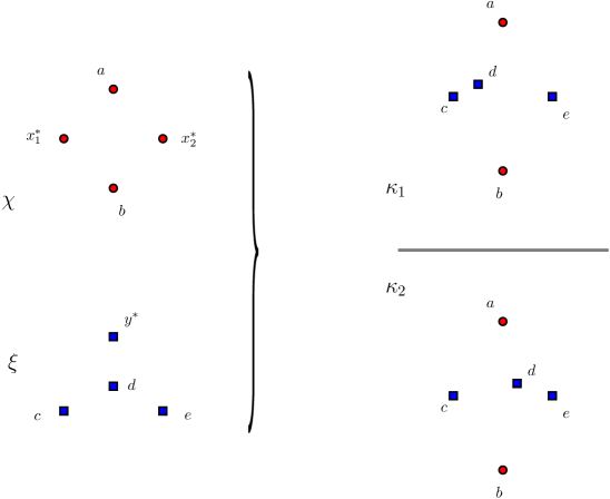
Figure 10. Two chirotopes $\kappa_{1}$ and $\kappa_{2}$ obtained from the same substitution (substituting $\xi$ into $\chi$ along the segment $x_{1}^{*}x_{2}^{*}$ squeezing $\xi$ orthogonally to $y^{*}$), but using different realizations. Observe that $d$ is not on the same side of the line $ab$ in $\kappa_{1}$ and $\kappa_{2}$.

Lemma 6.6.

For any realizable chirotope $\kappa$ on $Z$ and any quasi-module $Y$ of $\kappa$, there exist a single chirotope $\chi$ on $(Z\setminus Y)\cup\{x_{1}^{*},x_{2}^{*}\}$ and at most two chirotopes $\xi$ on $Y\cup\{y^{*}\}$ such that $\kappa$ can be obtained by the above construction (up to renaming the symbols $x_{1}^{*}$, $x_{2}^{*}$ and $y^{*}$).

Proof.

Suppose $\kappa$ and $Y$ are obtained by the above construction. Let $\{x_{1}^{*},x_{2}^{*}\}$ denote the antipodal elements of $Y$, defined through Lemma 6.3. Then, $\chi$ must coincide with the restriction of $\kappa$ to $(Z\setminus Y)\cup\{x_{1}^{*},x_{2}^{*}\}$, so it is unique (up to renaming the symbols $x_{1}^{*}$ and $x_{2}^{*}$).

Since $x_{1}^{*},x_{2}^{*}\in Y$ and $Y$ is a quasi-module of $\kappa$, this pair defines a nontrivial bipartition, so there exist $y^{*}_{+}$ and $y^{*}_{-}$ in $(Z\setminus Y)$ such that $\chi(x_{1}^{*},x_{2}^{*},y^{*}_{-})=-1$ and $\chi(x_{1}^{*},x_{2}^{*},y^{*}_{+})=+1$. By construction, $\xi$ must coincide with the restriction of $\kappa$ to $Y\cup\{y^{*}_{-}\}$ or to $Y\cup\{y^{*}_{+}\}$. There is therefore at most two choices for the chirotope $\xi$ on $Y\cup\{y^{*}\}$ (up to renaming the symbol $y^{*}$). ∎

We now use this construction for counting purposes. Let $w_{n,k}$ denote the number of pairs $(\chi,W)$ where $\chi$ is a realizable chirotope on $[n]$ and $W$ is a quasi-module of $\chi$ of size $k$. Recall that $t_{n}^{*}$ denotes the number of realizable chirotopes on $[n]$ in which $n$ is extreme. Let $t_{n}^{\div}$ denote the number of realizable chirotopes on $[n]$ in which $n$ and $n-1$ do not form an extreme edge.

Lemma 6.7.

For any integers $n_{1}\geq 2$, $n_{2}\geq 2$, we have $w_{n_{1}+n_{2},n_{2}}\geq\frac{1}{2}\binom{n_{1}+n_{2}}{n_{1}}t_{n_{1}+2}^{\div}t_{n_{2}+1}^{*}$.

Proof.

Let $n=n_{1}+n_{2}$. Start with a triple $(I,\chi,\xi)$ where $I\subset[n]$ has size $n_{1}$, $\chi$ is a realizable chirotope on $[n_{1}+2]$ such that $n_{1}+1$ and $n_{1}+2$ do not form an extreme edge, and $\xi$ is a realizable chirotope on $[n_{2}+1]$ in which $n_{2}+1$ is extreme. With our notations, the number of such triples is $\binom{n_{1}+n_{2}}{n_{1}}t_{n_{1}+2}^{\div}t_{n_{2}+1}^{*}$.

Let $x_{1}^{*},x_{2}^{*}$ and $y^{*}$ be formal symbols not in $[n]$. For each such triple $(I,\chi,\xi)$, we do the following operation:

• We let $\tilde{\chi}$ denote the chirotope on $I\cup\{x_{1}^{*},x_{2}^{*}\}$ obtained from $\chi$ by relabeling $[n_{1}]$ increasingly into $I$ and mapping $n_{1}+1\mapsto x_{1}^{*}$ and $n_{1}+2\mapsto x_{2}^{*}$.

• We let $\tilde{\xi}$ denote the chirotope on $([n]\setminus I)\cup\{y^{*}\}$ obtained from $\xi$ by relabeling $[n_{2}]$ increasingly into $[n]\setminus I$ and mapping $n_{2}+1\mapsto y^{*}$.

• We substitute $\tilde{\xi}$ into $\tilde{\chi}$ along the segment $x_{1}^{*}x_{2}^{*}$ squeezing $\tilde{\xi}$ orthogonally to $y^{*}$.

The result of this operation is a pair $(\kappa,W)$ where $\kappa$ is a realizable chirotope on $[n]$ and $W$ is a quasi-module. By Lemma 6.6, each pair $(\kappa,W)$ is the image of at most two triples $(I,\chi,\xi)$, which concludes the proof. ∎

We can now complete the proof of Lemma 5.7, that is, that for $n\geq\frac{3}{\varepsilon}$,

$$t_{n}\geq\frac{3K\varepsilon^{7}}{4}\,n^{3}\,d^{\rm large}_{n}\qquad\text{where}\qquad d^{\rm large}_{n}=\sum_{\begin{subarray}{c}n_{1}+n_{2}=n\\ \varepsilon n\leq n_{1},n_{2}\leq (1-\varepsilon)n\end{subarray}}\binom{n}{n_{1}}\,\frac{t_{n_{1}+1}\,t_{n_{2}+1}}{(n_{1}+1)\,(n_{2}+1)}.$$

Proof of Lemma 5.7.

Lemma 5.4 gives that $t_{n}^{*}\geq\frac{3}{n}t_{n}$. Furthermore, adapting the proof of Lemma 5.4 yields

$$\frac{t_{n}^{\div}}{t_{n}}=\frac{2}{n(n-1)}\mathbb{E}[\mathrm{nee}(\chi)]$$

where $\mathrm{nee}(\chi)$ denotes the number of pairs of points of $\chi$ which are not extreme edges. For $n\geq 5$, we have

$$\mathbb{E}[\mathrm{nee}(\chi)]\geq\binom{n}{2}-n\geq\frac{1}{2}\binom{n}{2}$$

and hence $t_{n}^{\div}\geq\frac{1}{2}t_{n}$. Now, by Lemmas 6.2 and 6.7 we have

$$\frac{n^{2}}{\varepsilon^{2}}t_{n}\geq\sum_{\begin{subarray}{c}n_{1}+n_{2}=n\\ \varepsilon n\leq n_{1},n_{2}\leq (1-\varepsilon)n\end{subarray}}w_{n,n_{2}} \geq\sum_{\begin{subarray}{c}n_{1}+n_{2}=n\\ \varepsilon n\leq n_{1},n_{2}\leq (1-\varepsilon)n\end{subarray}}\frac{1}{2}\binom{n}{n_{1}}t_{n_{1}+2}^{\div}t_{n_{2}+1}^{*}$$

$$\geq\sum_{\begin{subarray}{c}n_{1}+n_{2}=n\\ \varepsilon n\leq n_{1},n_{2}\leq (1-\varepsilon)n\end{subarray}}\frac{3}{4(n_{2}+1)}\binom{n}{n_{1}}t_{n_{1}+2}t_{n_{2}+1}.$$

(The inequality $t_{n_{1}+2}^{\div}\geq\frac{1}{2}t_{n_{1}+2}$ requires $n_{1}+2\geq 5$, which is ensured by the assumption $n\geq\frac{3}{\varepsilon}$.) By Lemma 5.3, there exists a universal constant $K>0$ such that, for all $n_{1}\geq 2$, we have $t_{n_{1}+2}\geq K\,(n_{1}+1)^{4}\,t_{n_{1}+1}$. Substituting into the previous inequality and using that $n_{1}+1\geq\varepsilon n$, we obtain as desired

$$t_{n} \geq\frac{\varepsilon^{2}}{n^{2}}\frac{3K}{4}\sum_{\begin{subarray}{c}n_{1}+n_{2}=n\\ \varepsilon n\leq n_{1},n_{2}\leq (1-\varepsilon)n\end{subarray}}\binom{n}{n_{1}}(n_{1}+1)^{5}\frac{t_{n_{1}+1}t_{n_{2}+1}}{(n_{1}+1)(n_{2}+1)}$$

$$\geq\varepsilon^{7}n^{3}\frac{3K}{4}\sum_{\begin{subarray}{c}n_{1}+n_{2}=n\\ \varepsilon n\leq n_{1},n_{2}\leq (1-\varepsilon)n\end{subarray}}\binom{n}{n_{1}}\frac{t_{n_{1}+1}t_{n_{2}+1}}{(n_{1}+1)(n_{2}+1)}.\qed$$

7. A bijection to decompose triangulations through one bowtie product

In this section, we consider a decomposable chirotope $\kappa=\chi\mathchoice{\sideset{{}_{x^{*}}}{{}_{y^{*}}}{\operatorname{\textup{\Bowtie}}}}{\sideset{{}_{x^{*}}}{{}_{y^{*}}}{\operatorname{\textup{\Bowtie}}}}{\sideset{{}_{x^{*}}}{{}_{y^{*}}}{\scriptstyle\operatorname{\textup{\Bowtie}}}}{\sideset{{}_{x^{*}}}{{}_{y^{*}}}{\scriptstyle\operatorname{\textup{\Bowtie}}}}\xi$, and relate the triangulations of $\kappa$ to those of $\chi$ and $\xi$. We show that each triangulation of $\kappa$ projects into triangulations of $\chi$ and $\xi$, and that conversely every pair of triangulations of $\chi$ and $\xi$ can be obtained as projections of (possibly many) triangulations of $\kappa$. We establish a bijection between these pre-images and maximal crossing-free matchings between two concave chains.

7.1. Statement of the bijection

Let $\kappa=\chi\mathchoice{\sideset{{}_{x^{*}}}{{}_{y^{*}}}{\operatorname{\textup{\Bowtie}}}}{\sideset{{}_{x^{*}}}{{}_{y^{*}}}{\operatorname{\textup{\Bowtie}}}}{\sideset{{}_{x^{*}}}{{}_{y^{*}}}{\scriptstyle\operatorname{\textup{\Bowtie}}}}{\sideset{{}_{x^{*}}}{{}_{y^{*}}}{\scriptstyle\operatorname{\textup{\Bowtie}}}}\xi$ where $\chi$ and $\xi$ are chirotopes on $X\cup\{x^{*}\}$ and $Y\cup\{y^{*}\}$, with $X$ and $Y$ disjoint, $x^{*}\notin X$ and $y^{*}\notin Y$.

Let $\pi_{Y\to x}$ denote the map that sends every element of $Y$ to $x$. We extend this map to sets of edges by putting, for any triangulation $T$ of $\kappa$,

$$\pi_{Y\to x}(T)\stackrel{{\scriptstyle\text{def}}}{{=}}\{\{\pi_{Y\to x}(a),\pi_{Y\to x}(b)\}\colon\{a,b\}\in T\}\setminus\{\{x,x\}\}.$$

We define $\pi_{X\to y^{*}}$ analogously. Given a set of edges $T$ of $\chi\mathchoice{\sideset{{}_{x^{*}}}{{}_{y^{*}}}{\operatorname{\textup{\Bowtie}}}}{\sideset{{}_{x^{*}}}{{}_{y^{*}}}{\operatorname{\textup{\Bowtie}}}}{\sideset{{}_{x^{*}}}{{}_{y^{*}}}{\scriptstyle\operatorname{\textup{\Bowtie}}}}{\sideset{{}_{x^{*}}}{{}_{y^{*}}}{\scriptstyle\operatorname{\textup{\Bowtie}}}}\xi$, not necessarily a triangulation, and two sets $A$ and $B$, we let $T_{AB}$ denote the set of edges of $T$ with one element in $A$ and the other in $B$; we say that such an edge is between $A$ and $B$. As illustrated in Figure 11, any triangulation $T$ of $\kappa$ decomposes into triangulations of $\chi$ and $\xi$ and a set $T_{XY}$ of non-crossing edges. The aim of this section is to prove that this decomposition is a bijection.

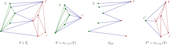
Figure 11. A triangulation $T$ of $\kappa=\chi\mathchoice{\sideset{{}_{x^{*}}}{{}_{y^{*}}}{\operatorname{\textup{\Bowtie}}}}{\sideset{{}_{x^{*}}}{{}_{y^{*}}}{\operatorname{\textup{\Bowtie}}}}{\sideset{{}_{x^{*}}}{{}_{y^{*}}}{\scriptstyle\operatorname{\textup{\Bowtie}}}}{\sideset{{}_{x^{*}}}{{}_{y^{*}}}{\scriptstyle\operatorname{\textup{\Bowtie}}}}\xi$, the projection of $T$ on $X\cup\{x^{*}\}$, the set $T_{XY}$, and the projection of $T$ on $Y\cup\{y^{*}\}$.

Recall that ${\cal T}_{\alpha}$ denotes the set of triangulations of a chirotope $\alpha$. Given $T\in{\cal T}_{\alpha}$ and a label $x$ of $\alpha$, we write $N_{T}(x)$ for the neighborhood of $x$ in $T$ and $\deg_{T}(x)$ for the degree of $x$ in $T$.

Proposition 7.1.

For any triangulation $T$ of $\kappa$, the sets $T^{\prime}\stackrel{{\scriptstyle\text{def}}}{{=}}\pi_{Y\to x^{*}}(T)$ and $T^{\prime\prime}\stackrel{{\scriptstyle\text{def}}}{{=}}\pi_{X\to y^{*}}(T)$ are triangulations of $\chi$ and $\xi$, respectively, and $T_{XY}$ is a maximal set of noncrossing edges between $N_{T^{\prime}}(x^{*})$ and $N_{T^{\prime\prime}}(y^{*})$.

Conversely, for any triangulations $T^{\prime}$ of $\chi$ and $T^{\prime\prime}$ of $\xi$ and any maximal set $H$ of non-crossing edges between $N_{T^{\prime}}(x^{*})$ and $N_{T^{\prime\prime}}(y^{*})$, there exists a unique triangulation $T\in{\mathcal{T}}_{\kappa}$ such that $T^{\prime}=\pi_{Y\to x^{*}}(T)$, $T^{\prime\prime}=\pi_{X\to y^{*}}(T)$ and $H=T_{XY}$.

The proof of the bijection studies in particular the geometric structure of the sets of non-crossing edges $T_{XY}$ for any triangulation of $\kappa$; from this structure we derive the following combinatorial combinatorial lemma that will be useful for counting triangulations.

Lemma 7.2.

Let $X^{\prime}\subseteq X$, $Y^{\prime}\subseteq Y$ be two non-empty subsets of elements of $\kappa$, with $z_{1},z_{2},\ldots,z_{k}\in Y^{\prime}$ , $k\geq 0$, and $|Y^{\prime}|\geq k+1$. Then for $i_{1},\ldots,i_{k}\geq 1$ there are exactly

$$\binom{|X^{\prime}|+|Y^{\prime}|-(i_{1}+\ldots+i_{k})-2}{|Y^{\prime}|-(k+1)}$$

maximal sets $H$ of edges between $X^{\prime}$ and $Y^{\prime}$, noncrossing in $\kappa$, and satisfying $\deg_{H}(z_{j})=i_{j}$ for every $j\in[k]$.

In particular, for $k=0$ obtain that for any non-empty subsets $X^{\prime}\subseteq X$ and $Y^{\prime}\subseteq Y$ there are exactly $\binom{|X^{\prime}|+|Y^{\prime}|-2}{|Y^{\prime}|-1}$ maximal sets $H$ of noncrossing edges in $\kappa$.

The rest of this section is devoted to proving Proposition 7.1 and Lemma 7.2.

7.2. Preparation: radial orderings and crossings

A classical consequence of Euler’s formula, via double counting, is that any triangulation $T$ of a realizable chirotope of size $n$ with $h$ extreme elements has exactly

(22) $$|T|=3n-h-3$$

edges. In particular, any family of noncrossing edges of a realizable chirotope of size $n$ with $h$ extreme elements has at most $3n-h-3$ edges. The fact that Equation (22) also holds for abstract chirotopes follows from the fact that every abstract chirotope can be realized by a generalized configuration, that is a set of points in the plane together with an arrangement of pseudolines, each one containing exactly two points [FG17, Theorems 5.2.6].

For a chirotope $\alpha$ on a set $A$, we write $\mathrm{ext}(\alpha)$ for the set of elements of $A$ that are extreme in $\alpha$. For $a,b,c\in A$ we write

$$b<_{\alpha,a}c\Leftrightarrow\alpha(a,b,c)=1.$$

If $a$ is extreme for $\alpha$, then $<_{\alpha,a}$ defines a strict total order on $A\setminus\{a\}$. Indeed, given $x,y,z\in X\setminus\{a\}$ such that $x<_{\alpha,a}y$ and $y<_{\alpha,a}z$, we have $\alpha(a,x,y)=\alpha(a,y,z)=1$ and the assumption that $a$ is extreme forces, with Lemma 2.1, that $\alpha(a,z,x)=-1$, that is $x<_{\alpha,a}z$.

Lemma 7.3.

Let $\chi$ and $\xi$ be chirotopes on $X\cup\{x^{*}\}$ and $Y\cup\{y^{*}\}$, with $X$ and $Y$ disjoint, $x^{*}\notin X$ and $y^{*}\notin Y$. Suppose that $x^{*}$ is extreme in $\chi$ and $y^{*}$ is extreme in $\xi$, and let $\kappa=\chi\mathchoice{\sideset{{}_{x^{*}}}{{}_{y^{*}}}{\operatorname{\textup{\Bowtie}}}}{\sideset{{}_{x^{*}}}{{}_{y^{*}}}{\operatorname{\textup{\Bowtie}}}}{\sideset{{}_{x^{*}}}{{}_{y^{*}}}{\scriptstyle\operatorname{\textup{\Bowtie}}}}{\sideset{{}_{x^{*}}}{{}_{y^{*}}}{\scriptstyle\operatorname{\textup{\Bowtie}}}}\xi$.

• For any set $T$ of noncrossing edges in $\kappa$, $\pi_{Y\to x^{*}}(T)$ is a set of noncrossing edges in $\chi$.

• For any $x_{1},x_{2}\in X$ and $y_{1},y_{2}\in Y$ with $y_{1}<_{\xi,y^{*}}y_{2}$, the edges $x_{1}y_{1}$ and $x_{2}y_{2}$ cross in $\chi\mathchoice{\sideset{{}_{x^{*}}}{{}_{y^{*}}}{\operatorname{\textup{\Bowtie}}}}{\sideset{{}_{x^{*}}}{{}_{y^{*}}}{\operatorname{\textup{\Bowtie}}}}{\sideset{{}_{x^{*}}}{{}_{y^{*}}}{\scriptstyle\operatorname{\textup{\Bowtie}}}}{\sideset{{}_{x^{*}}}{{}_{y^{*}}}{\scriptstyle\operatorname{\textup{\Bowtie}}}}\xi$ if and only if $x_{1}<_{\chi,x^{*}}x_{2}$.

Proof.

For the proof of Statement (i), recall that whether two edges cross or not in $\chi$ depends only on the restriction of the chirotope $\chi$ to the four endpoints of these two edges. Let $T^{\prime}=\pi_{Y\to x^{*}}(T)$. As $\chi$ and $\kappa$ coincide on $X$, no two edges of $T_{XX}$ can cross in $T^{\prime}$. Furthermore, by definition of $\pi_{Y\to x^{*}}$ and $\kappa$, the existence of two crossing edges $x^{*}x_{1}$ and $x_{2}x_{3}$ of $T^{\prime}$ (in $\chi$) would lead to the existence of an edge $y_{1}x_{1}\in T$ crossing the edge $x_{2}x_{3}\in T$ (in $\kappa$), with $y_{1}\in Y$, which is impossible since $T$ is a set of noncrossing edges in $\kappa$. This proves (i).

Now to statement (ii). By definition, we have $\chi(x^{*},x_{1},x_{2})=\kappa(x_{2},y_{2},x_{1})=-\kappa(x_{1},y_{1},x_{2})$ and similarly, we have $\xi(y^{*},y_{1},y_{2})=-\kappa(x_{2},y_{2},y_{1})=\kappa(x_{1},y_{1},y_{2})$, with $\xi(y^{*},y_{1},y_{2})=1$ by hypothesis. Hence if $x_{1}<_{\chi,x^{*}}x_{2}$, then $\kappa(x_{2},y_{2},x_{1})=-\kappa(x_{2},y_{2},y_{1})=1$ and $\kappa(x_{1},y_{1},x_{2})=-\kappa(x_{1},y_{1},y_{2})=-1$, so that $x_{1}y_{1}$ and $x_{2}y_{2}$ cross in $\kappa$. Conversely, if $x_{1}y_{1}$ and $x_{2}y_{2}$ cross, in particular $\kappa(x_{1},y_{1},x_{2})=-\kappa(x_{1},y_{1},y_{2})$, hence $1=\xi(y^{*},y_{1},y_{2})=-\chi(x_{1},x^{*},x_{2})=\chi(x^{*},x_{1},x_{2})$ and $x_{1}<_{\chi,x^{*}}x_{2}$. This proves Statement (ii). ∎

Lemma 7.4.

Let $X^{\prime}\subseteq X$, $Y^{\prime}\subseteq Y$ be two non-empty subsets of elements of $\kappa$. Let us write $a=|X^{\prime}|$, $b=|Y^{\prime}|$, and $y_{1}<_{\xi,y^{*}}\ldots<_{\xi,y^{*}}y_{b}$ the elements of $Y^{\prime}$. The map $H\mapsto(\deg_{H}(y_{1}),\ldots,\deg_{H}(y_{b}))$ is a bijection between the maximal sets of edges between $X^{\prime}$ and $Y^{\prime}$ and noncrossing in $\kappa$, and the sequences $(d_{1},\ldots,d_{b})\in\left({\mathbb{N}}_{\geq 1}\right)^{b}$ satisfying $d_{1}+\ldots+d_{b}=a+b-1$.

Proof.

Let us write $x_{1}<_{\chi,x^{*}}\ldots<_{\chi,x^{*}}x_{a}$ the elements of $X^{\prime}$, ordered by $<_{\chi,x^{*}}$. Let $\Lambda_{a,b}$ denote the set of sequences $(d_{1},\ldots,d_{b})\in\left({\mathbb{N}}_{\geq 1}\right)^{b}$ satisfying $d_{1}+\ldots+d_{b}=a+b-1$.

Let $H$ be a maximal set of edges between $X^{\prime}$ and $Y^{\prime}$ that is non-crossing for $\kappa$. For $j\in[b]$, we let ${\cal I}^{H}_{j}$ denote the set of indices $i$ such that $x_{i}y_{j}$ is an edge of $H$. By maximality of $H$, every element of $Y^{\prime}$ is the endpoint of an edge, so each set ${\cal I}^{H}_{j}$ is non-empty; we let $m_{j}$ and $M_{j}$ denote its minimal and maximal elements. Again by maximality of $H$, every element of $X^{\prime}$ is the endpoint of an edge, so the union of ${\cal I}^{H}_{j}$ is $[a]$. By Lemma 7.3 (ii), if for some $i\in{\cal I}^{H}_{t}$ we have $m_{j}<i<M_{j}$, then we cannot have $t>j$ (as otherwise $x_{t}y_{i}$ crosses $x_{j}y_{m_{j}}$) nor have $t<j$ (as otherwise $x_{t}y_{i}$ crosses $x_{j}y_{M_{j}}$). It follows that ${\cal I}^{H}_{j}=[m_{j},M_{j}]$ and, by the maximality of $H$, that consecutive ${\cal I}^{H}_{j}$ have a common endpoint. In other words, we have

$$1=m_{b}\leq M_{b}=m_{b-1}\leq M_{b-1}=\ldots=m_{2}\leq M_{2}=m_{1}\leq M_{1}=a.$$

Since $\deg_{H}(y_{j})=M_{j}-m_{j}+1=m_{j-1}-m_{j}+1$, it follows that the map sending $H$ to $(\deg_{H}(y_{1}),\ldots,\deg_{H}(y_{b}))$ is an injection into $\Lambda_{a,b}$.

Conversely, for any sequence $S=(d_{i})\in\Lambda_{a,b}$, we let $H_{S}$ denote the set $H$ of edges defined as follows. We start with an empty set of edges and add an edge between $y_{b}$ and each of $x_{1},\ldots,x_{d_{1}}$, the first $d_{1}$ elements of $X^{\prime}$; then we add an edge between $y_{b-1}$ and each of the next $d_{2}$ elements of $X^{\prime}$, starting from $x_{d_{1}}$ included. Et caetera. The edges of $H_{S}$ are non-crossing by Lemma 7.3 (ii). Moreover, for every $j\in[b]$ we have $N_{H_{S}}(y_{j})=[m_{j},m_{j-1}]$ where $m_{b}=1$ and $m_{j-1}=m_{j}+d_{j}-1$, so the map $S\to H_{S}$ is injective. As argued above, no edge can be added to $H_{S}$ without crossing in $\kappa$ an edge already present, so $H_{S}$ is indeed maximal. ∎

We can then deduce the following lemma.

Lemma 7.2. Let $X^{\prime}\subseteq X$, $Y^{\prime}\subseteq Y$ be two non-empty subsets of elements of $\kappa$, with $z_{1},z_{2},\ldots,z_{k}\in Y^{\prime}$ , $0\leq k<b$, and $|Y^{\prime}|\geq k+1$. Then for $i_{1},\ldots,i_{k}\geq 1$ there are exactly

$$\binom{|X^{\prime}|+|Y^{\prime}|-(i_{1}+\ldots+i_{k})-2}{|Y^{\prime}|-(k+1)}$$

maximal sets $H$ of edges between $X^{\prime}$ and $Y^{\prime}$, noncrossing in $\kappa$, and satisfying $\deg_{H}(z_{j})=i_{j}$ for every $j\in[k]$.

Proof.

By Lemma 7.4, it suffices to count the number of sequences $(m_{1},\ldots,m_{b})$ satisfying $m_{1}+\ldots+m_{b}=a+b-1$ with $m_{i}\in\mathbb{Z}_{\geq 1}$, and the value of $(m_{i})$ for the $k$ first indexes is fixed to be $i_{1},\ldots,i_{k}$ (we allow $k=0$). These sequences are in bijection with the sequences $(n_{1},\ldots,n_{b-k})$ of $b-k\geq 1$ positive integers summing to $a+b-1-(i_{1}+\ldots+i_{k})$, i.e. the compositions of $a+b-1-(i_{1}+\ldots+i_{k})$ into $b-k$ parts, which is counted by $\binom{a+b-(i_{1}+\ldots+i_{k})-2}{b-k-1}$. ∎

7.3. Proof of the bijection.

Observe that Lemma 7.4 implies that, with the notations of Proposition 7.1, any maximal set of edges between $X$ and $Y$ that are non-crossing for $\kappa$ has size $|X|+|Y|-1$. The first statement of our bijection (Proposition 7.1) thus reformulates as follows.

Proposition 7.5.

Let $\kappa=\chi\mathchoice{\sideset{{}_{x^{*}}}{{}_{y^{*}}}{\operatorname{\textup{\Bowtie}}}}{\sideset{{}_{x^{*}}}{{}_{y^{*}}}{\operatorname{\textup{\Bowtie}}}}{\sideset{{}_{x^{*}}}{{}_{y^{*}}}{\scriptstyle\operatorname{\textup{\Bowtie}}}}{\sideset{{}_{x^{*}}}{{}_{y^{*}}}{\scriptstyle\operatorname{\textup{\Bowtie}}}}\xi$. For any triangulation $T\in{\mathcal{T}}_{\kappa}$, the sets $T^{\prime}\stackrel{{\scriptstyle\text{def}}}{{=}}\pi_{Y\to x^{*}}(T)$ and $T^{\prime\prime}\stackrel{{\scriptstyle\text{def}}}{{=}}\pi_{X\to y^{*}}(T)$ are triangulations of, respectively, $\chi$ and $\xi$, and $T_{XY}$ is a set of $\deg_{T^{\prime}}(x^{*})+\deg_{T^{\prime\prime}}(y^{*})-1$ noncrossing edges between $N_{T^{\prime}}(x^{*})$ and $N_{T^{\prime\prime}}(y^{*})$.

Proof.

Let $T\in\mathcal{T}_{\kappa}$ be a triangulation of $\kappa$. The number of edges in $T$ is given by

$$|T|=|T_{XX}|+|T_{YY}|+|T_{XY}|.$$

Recall that $T^{\prime}=\pi_{Y\to x^{*}}(T)$ and $T^{\prime\prime}=\pi_{X\to y^{*}}(T)$ denote the projections of $T$ on respectively $\chi$ and $\xi$. Let us consider the set $X^{\prime}$ of elements of $X$ forming an edge in $T$ with at least one element of $Y$. Notice that by the definition of $\pi_{Y\to x^{*}}$, we have $X^{\prime}=N_{T^{\prime}}(x^{*})$, and in particular $|X^{\prime}|=\deg_{T^{\prime}}(x^{*})$. Similarly we can define $Y^{\prime}=N_{T^{\prime\prime}}(y^{*})$, and $|Y^{\prime}|=\deg_{T^{\prime\prime}}(y^{*})$. Hence

$$|T^{\prime}|=|T_{XX}|+\deg_{T^{\prime}}(x^{*})=|T_{XX}|+|X^{\prime}|,\quad|T^{\prime\prime}|=|T_{YY}|+|Y^{\prime}|\,.$$

As $T_{XY}$ is a set of noncrossing edges of $\kappa$ with one endpoint in $X^{\prime}\subseteq X$ and the other in $Y^{\prime}\subseteq Y$, we have by Lemma 7.4:

$$|T_{XY}|\leq|X^{\prime}|+|Y^{\prime}|-1\,.$$

Hence we have the following inequality:

$$|T|=|T_{XX}|+|T_{YY}|+|T_{XY}|\leq|T_{XX}|+|T_{YY}|+|X^{\prime}|+|Y^{\prime}|-1=|T^{\prime}|+|T^{\prime\prime}|-1.$$

Let $h_{X}$ (resp. $h_{Y}$) denote the number of elements of $X$ (resp. $Y$) that are extreme in $\kappa$. As $T$ is a triangulation of $\kappa$, by Equation 22 we have

$$|T|=3(|X|+|Y|)-(h_{X}+h_{Y})-3.$$

By Lemma 7.3 (i), $T^{\prime}$ and $T^{\prime\prime}$ are families of noncrossing edges of $\chi$ and $\xi$, hence by Equation 22,

$$|T^{\prime}|\leq 3(|X|+1)-(h_{X}+1)-3=3|X|-h_{X}-1\qquad\text{and}\qquad|T^{\prime\prime}|\leq 3|Y|-h_{Y}-1$$

so that

$$|T|\leq|T^{\prime}|+|T^{\prime\prime}|-1\leq 3(|X|+|Y|)-(h_{X}+h_{Y})-3=|T|.$$

This implies that every inequality we have proved so far is in fact an equality. In particular, $T^{\prime}$ (resp. $T^{\prime\prime}$) contains the maximal possible number of noncrossing edges of $\chi$ (resp. $\xi$), ensuring that it is a triangulation of $\chi$ (resp. $\xi$); and $|T_{XY}|=|X^{\prime}|+|Y^{\prime}|-1=\deg_{T^{\prime}}(x^{*})+\deg_{T^{\prime\prime}}(y^{*})-1$, concluding the proof. ∎

Similarly, Lemma 7.4 allows to reformulate the second statement of Proposition 7.1 as follows.

Proposition 7.6.

For any triangulations $T^{\prime}$ and $T^{\prime\prime}$ of, respectively, $\chi$ and $\xi$, and any set $H$ of $\deg_{T^{\prime}}(x^{*})+\deg_{T^{\prime\prime}}(y^{*})-1$ noncrossing edges between $N_{T^{\prime}}(x^{*})$ and $N_{T^{\prime\prime}}(y^{*})$, there exists a unique triangulation $T\in{\mathcal{T}}_{\kappa}$ such that $T^{\prime}=\pi_{Y\to x^{*}}(T)$, $T^{\prime\prime}=\pi_{X\to y^{*}}(T)$ and $H=T_{XY}$.

Proof.

If $T$ is a triangulation of $\kappa$ satisfying $\pi_{Y\to x^{*}}(T)=T^{\prime}$, $\pi_{X\to y^{*}}(T)=T^{\prime\prime}$ and $T_{XY}=H$, then $T$ is necessarily such that $T_{XX}=T^{\prime}_{XX}$, $T_{YY}=T^{\prime\prime}_{YY}$, and $T_{XY}=H$, and consequently $T$ is unique.

To prove the existence of $T$ under the assumptions of Proposition 7.6, let us thus define $T=T^{\prime}_{XX}\cup T^{\prime\prime}_{YY}\,\cup\,H$. By construction, $\pi_{Y\to x^{*}}(T)=T^{\prime}$, $\pi_{X\to y^{*}}(T)=T^{\prime\prime}$ and $T_{XY}=H$. In particular, $|T^{\prime}|=|T^{\prime}_{XX}|+\deg_{T^{\prime}}(x^{*})$ and $|T^{\prime\prime}|=|T^{\prime\prime}_{YY}|+\deg_{T^{\prime\prime}}(y^{*})$. Hence

$$|T|=|T^{\prime}|+|T^{\prime\prime}|-1\,.$$

We want to prove that $T$ is a triangulation of $\kappa$. First, let us prove that $T$ has the right number of edges. Let $h_{X}$ (resp. $h_{Y}$) denote the number of elements of $X$ (resp. $Y$) that are extreme in $\kappa$. Since $T^{\prime}$ and $T^{\prime\prime}$ are triangulations of respectively $\chi$ and $\xi$, by Equation 22,

$$|T^{\prime}|=3(|X|+1)-(h_{X}+1)-3=3|X|-h_{X}-1\qquad\text{and}\qquad|T^{\prime\prime}|=3|Y|-h_{Y}-1\,.$$

Hence $T$ has the right number of edges to be a triangulation, as we compute

$$|T|=3|X|-h_{X}-1+3|Y|-h_{Y}-1-1=3(|X|+|Y|)-(h_{X}+h_{Y})-3\,.$$

In order to show that $T$ is a triangulation of $\kappa$, it remains to prove that it consists of noncrossing edges. By hypothesis, the edges in $T^{\prime}_{XX}\subseteq T^{\prime}$ are pairwise noncrossing, and similarly for the edges in $T^{\prime\prime}_{YY}$, or in $H$. An edge in $T^{\prime}_{XX}$ cannot cross an edge in $T^{\prime\prime}_{YY}$ as $X$ and $Y$ are mutually avoiding sets in $\kappa$. Finally, an edge of $H$ cannot cross in $\kappa$ an edge of $T^{\prime}_{XX}$ (resp. $T^{\prime\prime}_{YY}$ by symmetry): suppose by contradiction that $x_{1}y_{1}\in H$ is crossing $x_{2}x_{3}\in T^{\prime}_{XX}$ in $\kappa$. Then it would imply that the edges $x_{1}x^{*}$ and $x_{2}x_{3}$ are two crossing edges in $T^{\prime}$, which is impossible as $T^{\prime}$ is a triangulation.∎

8. Counting triangulations

We now explain how to count the triangulations of a chirotope presented by a chirotope tree from information on the triangulations of the chirotopes decorating the nodes.

8.1. Counting the triangulations of a bowtie

Let us first consider the case of a single bowtie. Proposition 7.1 describes the set of triangulations of a chirotope presented as a bowtie in terms of the sets of triangulations of the parts. With Lemma 7.4, however, we can count the former knowing only the generating polynomials of the laters marking the degrees of the proxies.

Let $P_{\chi,x^{*}}(s)$ and $P_{\xi,y^{*}}(t)$ denote the generating polynomials of the triangulations of $\chi$ and $\xi$ recording, respectively, the degrees of the elements $x^{*}$ and $y^{*}$:

$$P_{\chi,x^{*}}(s)=\sum_{T^{\prime}\in\mathcal{T}_{\chi}}s^{\deg_{T^{\prime}}(x^{*})}\qquad\text{and}\qquad P_{\xi,y^{*}}(t)=\sum_{T^{\prime\prime}\in\mathcal{T}_{\xi}}t^{\deg_{T^{\prime\prime}}(y^{*})}.$$

Here are examples with $P_{\chi,x^{*}}(s)=s^{3}(s+1)$ and $P_{\xi,y^{*}}(t)=t^{2}(1+t+t^{2})$.

The bijection of Proposition 7.1 implies Formula (6) which expresses $|{\cal T}_{\kappa}|$ for $\kappa\stackrel{{\scriptstyle\text{def}}}{{=}}\chi\mathchoice{\sideset{{}_{x^{*}}}{{}_{y^{*}}}{\operatorname{\textup{\Bowtie}}}}{\sideset{{}_{x^{*}}}{{}_{y^{*}}}{\operatorname{\textup{\Bowtie}}}}{\sideset{{}_{x^{*}}}{{}_{y^{*}}}{\scriptstyle\operatorname{\textup{\Bowtie}}}}{\sideset{{}_{x^{*}}}{{}_{y^{*}}}{\scriptstyle\operatorname{\textup{\Bowtie}}}}\xi$ from $P_{\chi,x^{*}}(s)$ and $P_{\xi,y^{*}}(t)$.

Proposition 8.1.

Let $\kappa=\chi\mathchoice{\sideset{{}_{x^{*}}}{{}_{y^{*}}}{\operatorname{\textup{\Bowtie}}}}{\sideset{{}_{x^{*}}}{{}_{y^{*}}}{\operatorname{\textup{\Bowtie}}}}{\sideset{{}_{x^{*}}}{{}_{y^{*}}}{\scriptstyle\operatorname{\textup{\Bowtie}}}}{\sideset{{}_{x^{*}}}{{}_{y^{*}}}{\scriptstyle\operatorname{\textup{\Bowtie}}}}\xi$ where $\chi$ and $\xi$ are two chirotopes on disjoint ground sets $X\cup\{x^{*}\}$ and $Y\cup\{y^{*}\}$, respectively. The number of triangulations of $\kappa$ is

(6) $$|\mathcal{T}_{\kappa}|=\sum_{\begin{subarray}{c}T^{\prime}\in\mathcal{T}_{\chi}\\ T^{\prime\prime}\in\mathcal{T}_{\xi}\end{subarray}}\binom{\deg_{T^{\prime}}(x^{*})+\deg_{T^{\prime\prime}}(y^{*})-2}{\deg_{T^{\prime}}(x^{*})-1}=\sum_{a,b\geq 2}\binom{a+b-2}{a-1}[s^{a}]P_{\chi,x^{*}}(s)\ [t^{b}]P_{\xi,y^{*}}(t).$$

Proof.

Let $\mathcal{T}_{\mathchoice{\sideset{}{}{\operatorname{\textup{\Bowtie}}}}{\sideset{}{}{\operatorname{\textup{\Bowtie}}}}{\sideset{}{}{\scriptstyle\operatorname{\textup{\Bowtie}}}}{\sideset{}{}{\scriptstyle\operatorname{\textup{\Bowtie}}}}}$ denote the set of triples $(T^{\prime},T^{\prime\prime},H)$ such that $T^{\prime}\in\mathcal{T}_{\chi}$, $T^{\prime\prime}\in\mathcal{T}_{\xi}$ and $H$ is a set of $\deg_{T^{\prime}}(x^{*})+\deg_{T^{\prime\prime}}(y^{*})-1$ noncrossing edges between $N_{T^{\prime}}(x^{*})$ and $N_{T^{\prime\prime}}(y^{*})$. By Lemma 7.2 (case $k=0$), for fixed $T^{\prime}\in\mathcal{T}_{\chi}$ and $T^{\prime\prime}\in\mathcal{T}_{\xi}$, there are $\binom{\deg_{T^{\prime}}(x^{*})+\deg_{T^{\prime\prime}}(y^{*})-2}{\deg_{T^{\prime}}(x^{*})-1}$ possible sets $H$ such that $(T^{\prime},T^{\prime\prime},H)\in\mathcal{T}_{\mathchoice{\sideset{}{}{\operatorname{\textup{\Bowtie}}}}{\sideset{}{}{\operatorname{\textup{\Bowtie}}}}{\sideset{}{}{\scriptstyle\operatorname{\textup{\Bowtie}}}}{\sideset{}{}{\scriptstyle\operatorname{\textup{\Bowtie}}}}}$. By Propositions 7.5 and 7.6, $|\mathcal{T}_{\kappa}|=|\mathcal{T}_{\mathchoice{\sideset{}{}{\operatorname{\textup{\Bowtie}}}}{\sideset{}{}{\operatorname{\textup{\Bowtie}}}}{\sideset{}{}{\scriptstyle\operatorname{\textup{\Bowtie}}}}{\sideset{}{}{\scriptstyle\operatorname{\textup{\Bowtie}}}}}|$, hence:

$$|\mathcal{T}_{\kappa}|=\sum_{\begin{subarray}{c}T^{\prime}\in\mathcal{T}_{\chi}\\ T^{\prime\prime}\in\mathcal{T}_{\xi}\end{subarray}}\binom{\deg_{T^{\prime}}(x^{*})+\deg_{T^{\prime\prime}}(y^{*})-2}{\deg_{T^{\prime}}(x^{*})-1}=\sum_{a,b\geq 2}\binom{a+b-2}{a-1}[s^{a}]P_{\chi,x^{*}}(s)\ [t^{b}]P_{\xi,y^{*}}(t),$$

where the last equality is obtained by grouping triangulations according to the respective degrees of $x^{*}$ and $y^{*}$, which is always at least $2$ in any triangulation. ∎

8.2. Generating polynomial of the triangulations of a bowtie

We just used the bijection of Proposition 7.1 to express $|{\cal T}_{\kappa}|$ for $\kappa\stackrel{{\scriptstyle\text{def}}}{{=}}\chi\mathchoice{\sideset{{}_{x^{*}}}{{}_{y^{*}}}{\operatorname{\textup{\Bowtie}}}}{\sideset{{}_{x^{*}}}{{}_{y^{*}}}{\operatorname{\textup{\Bowtie}}}}{\sideset{{}_{x^{*}}}{{}_{y^{*}}}{\scriptstyle\operatorname{\textup{\Bowtie}}}}{\sideset{{}_{x^{*}}}{{}_{y^{*}}}{\scriptstyle\operatorname{\textup{\Bowtie}}}}\xi$ from $P_{\chi,x^{*}}(s)$ and $P_{\xi,y^{*}}(t)$ (see Formula (6)). To iterate this computation through several bowtie products, we need to determine not only $|{\cal T}_{\kappa}|$, but $P_{\kappa,z^{*}}(t)$ for some extreme point $z^{*}$ of $\kappa$, to be used as a proxy point in a subsequent bowtie product.

Note that at this point, $\chi$ and $\xi$ do not play a symmetric role anymore, as $z^{*}$ is an element of the ground sets of only one of them. Without loss of generality, we suppose that $z^{*}\in Y$, and we replace $P_{\xi,y^{*}}(t)$ by two bivariate polynomials:

$$Q^{\in}_{\xi,y^{*},z^{*}}(t,u)=\sum_{\begin{subarray}{c}T\in\mathcal{T}_{\xi}\\ \{y^{*},z^{*}\}\in T\end{subarray}}t^{\deg_{T}(y^{*})}u^{\deg_{T}(z^{*})}\quad\text{and}\quad Q^{\notin}_{\xi,y^{*},z^{*}}(t,u)=\sum_{\begin{subarray}{c}T\in\mathcal{T}_{\xi}\\ \{y^{*},z^{*}\}\notin T\end{subarray}}t^{\deg_{T}(y^{*})}u^{\deg_{T}(z^{*})}.$$

Note that $P_{\xi,y^{*}}(t)=Q^{\in}_{\xi,y^{*},z^{*}}(t,1)+Q^{\notin}_{\xi,y^{*},z^{*}}(t,1)$. In the example

we have $Q^{\in}_{\xi,y^{*},z^{*}}(t,u)=t^{4}u^{4}$ and $Q^{\notin}_{\xi,y^{*},z^{*}}(t,u)=t^{2}u^{3}(1+t)$. In the following proposition, we express $P_{\kappa,z^{*}}(u)$ from $Q^{\in}_{\xi,y^{*},z^{*}}(t,u)$ and $Q^{\notin}_{\xi,y^{*},z^{*}}(t,u)$.

Proposition 8.2.

Let $\kappa=\chi\mathchoice{\sideset{{}_{x^{*}}}{{}_{y^{*}}}{\operatorname{\textup{\Bowtie}}}}{\sideset{{}_{x^{*}}}{{}_{y^{*}}}{\operatorname{\textup{\Bowtie}}}}{\sideset{{}_{x^{*}}}{{}_{y^{*}}}{\scriptstyle\operatorname{\textup{\Bowtie}}}}{\sideset{{}_{x^{*}}}{{}_{y^{*}}}{\scriptstyle\operatorname{\textup{\Bowtie}}}}\xi$ where $\chi$ and $\xi$ are chirotopes on $X\cup\{x^{*}\}$ and $Y\cup\{y^{*}\}$, with $X$ and $Y$ disjoint, $x^{*}\notin X$ and $y^{*}\notin Y$. For any $z^{*}\in Y$ extreme in $\xi$ we have

$$P_{\kappa,z^{*}}(u)= \sum_{a,b\geq 2}\tbinom{a+b-2}{a-1}[s^{a}]P_{\chi,x^{*}}(s)[t^{b}]Q^{\notin}_{\xi,y^{*},z^{*}}(t,u)$$

$$+\sum_{a,b\geq 2}R_{a,b}(u)[s^{a}]P_{\chi,x^{*}}(s)\ [t^{b}]Q^{\in}_{\xi,y^{*},z^{*}}(t,u),\text{ with }R_{a,b}(u)=\sum_{i=0}^{a-1}\tbinom{a+b-i-3}{b-2}u^{i}.$$

Proof.

The proof relies on the bijection of Proposition 7.1. For $T\in\mathcal{T}_{\kappa}$ a triangulation of $\kappa$, we let $T^{\prime}=\pi_{Y\to x^{*}}(T)$ and $T^{\prime\prime}=\pi_{X\to y^{*}}(T)$. We recall that $T_{XY}$ denotes the set of edges in $T$ joining $X$ to $Y$. Notice that there is an edge in $T$ between $z^{*}$ and an element of $X$ if and only if $\{y^{*},z^{*}\}\in T^{\prime\prime}$ (see Figure 11).

The contribution of a triangulation $T\in\mathcal{T}_{\kappa}$ to $P_{\kappa,z^{*}}(u)$ depends on whether it contains an edge between $z^{*}$ and an element of $X$. We let $\mathcal{T}_{\kappa}^{\in}$ (resp.$\mathcal{T}_{\kappa}^{\notin}$) denote the set of triangulations of $\mathcal{T}_{\kappa}$ that contain (resp. do not contain) an edge between $z^{*}$ and an element of $X$.

For any $T\in\mathcal{T}^{\notin}$, we have $\deg_{T}(z^{*})=\deg_{T^{\prime\prime}}(z^{*})$ as $\{y^{*},z^{*}\}\notin T^{\prime\prime}$ (see Figure 11) so that the contribution of every triangulation of $\mathcal{T}^{\notin}$ to $P_{\kappa,z^{*}}(u)$ can then be computed by a straightforward adaptation of Corollary 8.1:

$$\sum_{T\in\mathcal{T}^{\notin}_{\kappa}}u^{\deg_{T}(z^{*})}=\sum_{a,b\geq 2}\binom{a+b-2}{a-1}[s^{a}]P_{\chi,x^{*}}(s)\ [t^{b}]Q^{\notin}_{\xi,y^{*},z^{*}}(t,u)\,.$$

Now, assume that $T\in\mathcal{T}^{\in}$, so that $\{y^{*},z^{*}\}\in T^{\prime\prime}$. The edges incident to $z^{*}$ in $T$ are exactly the union of those incident to $z^{*}$ in $T_{XY}$ and those incident to $z^{*}$ in $T^{\prime\prime}$, minus the edge $\{y^{*},z^{*}\}$ (see Figure 11). Hence $\deg_{T}(z^{*})=\deg_{T_{XY}}(z^{*})+\deg_{T^{\prime\prime}}(z^{*})-1$. Using Lemma 7.2 (case $k=1$) after regrouping the terms according to the value of $i=\deg_{T_{XY}}(z^{*})$, we obtain:

$$\sum_{T\in\mathcal{T}^{\in}_{\kappa}}u^{\deg_{T}(z^{*})}=\sum_{\begin{subarray}{c}T^{\prime}\in\mathcal{T}_{\chi}\\ T^{\prime\prime}\in\mathcal{T}_{\xi},\,\{y^{*},z^{*}\}\in T^{\prime\prime}\end{subarray}}u^{\deg_{T^{\prime\prime}}(z^{*})}\underbrace{\sum_{i=1}^{\deg_{T^{\prime}}(x^{*})}\binom{\deg_{T^{\prime}}(x^{*})+\deg_{T^{\prime\prime}}(y^{*})-i-2}{\deg_{T^{\prime\prime}}(y^{*})-2}u^{i-1}}_{=R_{\deg_{T^{\prime}}(x^{*}),\deg_{T^{\prime\prime}}(y^{*})}(u)}\,.$$

Grouping the terms by the values of $a=\deg_{T^{\prime}}(x^{*})\geq 2$ and $b=\deg_{T^{\prime\prime}}(y^{*})\geq 2$, we finally obtain

$$\sum_{T\in\mathcal{T}^{\in}_{\kappa}}u^{\deg_{T}(z^{*})}=\sum_{a,b\geq 2}R_{a,b}(u)[s^{a}]P_{\chi,x^{*}}(s)\ [t^{b}]Q^{\in}_{\xi,y^{*},z^{*}}(t,u)\,,$$

concluding the proof. ∎

8.3. Illustration: triangulations of a family of chirotope chains

Let us give some example of a family of chirotope chains for which the analysis can be fully carried out using tools from analytic combinatorics.

Consider the two following chirotopes on $\{x^{*},y^{*},z,c\}$:

$\chi^{(0)}=$   and   $\chi^{(1)}=$

Each of $\chi^{(0)}$ and $\chi^{(1)}$ has a unique triangulation, which contains the edge $\{x^{*},y^{*}\}$ and where each vertex has degree $3$. Thus,

$$\begin{array}[]{ccccl}P_{\chi^{(0)},y^{*}}(s)&=&P_{\chi^{(1)},y^{*}}(s)&=&s^{3},\\ Q_{\chi^{(0)},x^{*},y^{*}}^{\in}(t,u)&=&Q_{\chi^{(1)},x^{*},y^{*}}^{\in}(t,u)&=&t^{3}u^{3},\\ Q_{\chi^{(0)},x^{*},y^{*}}^{\notin}(t,u)&=&Q_{\chi^{(1)},x^{*},y^{*}}^{\notin}(t,u)&=&0.\end{array}$$

For $i\in\mathbb{N}$, let $\chi_{i}^{(0)}$ denote a copy of $\chi^{(0)}$ relabeled by $x^{*}\mapsto x_{i}^{*}$, $y^{*}\mapsto y_{i}^{*}$, $z\mapsto z_{i}$, $c\mapsto c_{i}$. We define $\chi_{i}^{(1)}$ to be a copy of $\chi^{(1)}$ with the same relabeling. For any word $\sigma=\sigma_{1}\sigma_{2}\ldots\sigma_{k}\in\{0,1\}^{k}$ we put $\chi^{(\sigma)}\stackrel{{\scriptstyle\text{def}}}{{=}}\chi_{1}^{(\sigma_{1})}\mathchoice{\sideset{{}_{y_{1}^{*}}}{{}_{x_{2}^{*}}}{\operatorname{\textup{\Bowtie}}}}{\sideset{{}_{y_{1}^{*}}}{{}_{x_{2}^{*}}}{\operatorname{\textup{\Bowtie}}}}{\sideset{{}_{y_{1}^{*}}}{{}_{x_{2}^{*}}}{\scriptstyle\operatorname{\textup{\Bowtie}}}}{\sideset{{}_{y_{1}^{*}}}{{}_{x_{2}^{*}}}{\scriptstyle\operatorname{\textup{\Bowtie}}}}\chi_{2}^{(\sigma_{2})}\mathchoice{\sideset{{}_{y_{2}^{*}}}{{}_{x_{3}^{*}}}{\operatorname{\textup{\Bowtie}}}}{\sideset{{}_{y_{2}^{*}}}{{}_{x_{3}^{*}}}{\operatorname{\textup{\Bowtie}}}}{\sideset{{}_{y_{2}^{*}}}{{}_{x_{3}^{*}}}{\scriptstyle\operatorname{\textup{\Bowtie}}}}{\sideset{{}_{y_{2}^{*}}}{{}_{x_{3}^{*}}}{\scriptstyle\operatorname{\textup{\Bowtie}}}}\ldots\mathchoice{\sideset{{}_{y_{k-1}^{*}}}{{}_{x_{k}^{*}}}{\operatorname{\textup{\Bowtie}}}}{\sideset{{}_{y_{k-1}^{*}}}{{}_{x_{k}^{*}}}{\operatorname{\textup{\Bowtie}}}}{\sideset{{}_{y_{k-1}^{*}}}{{}_{x_{k}^{*}}}{\scriptstyle\operatorname{\textup{\Bowtie}}}}{\sideset{{}_{y_{k-1}^{*}}}{{}_{x_{k}^{*}}}{\scriptstyle\operatorname{\textup{\Bowtie}}}}\chi_{k}^{(\sigma_{k})}$. This expression translates into a chirotope tree, actually a chain, for example for $\chi^{(01101)}$:

The chirotopes $\chi^{(0)}$ and $\chi^{(1)}$ are indecomposable (and non-convex), so these trees are canonical and Theorem 1.3 ensures that $\chi^{(\sigma)}=\chi^{(\sigma^{\prime})}$ if and only if $\sigma=\sigma^{\prime}$. Moreover, $\chi^{(0)}$ and $\chi^{(1)}$ are realizable so $\chi^{(\sigma)}$ is realizable by Proposition 1.1 (ii) and is the chirotope of a set of $2k+2$ points, $k$ of which are interior. It turns out that the number of triangulations of $\chi^{(\sigma)}$ depends only on the length of $\sigma$, and there is a closed formula for this number!

Proposition 8.3.

For every $\sigma\in\{0,1\}^{k}$ we have

$$\left|{\cal T}_{\chi^{(\sigma)}}\right|=\frac{3(2k+1){\binom{4k+2}{2k+1}}}{(2k+2)(4k+1)}-\frac{{4}^{k}{\binom{2k+2}{k+1}}}{2k+1}\sim_{k\to\infty}\frac{3-2\sqrt{2}}{\sqrt{2\pi}}\frac{16^{k}}{k^{3/2}}.$$

Recall that for $\sigma\in\{0,1\}^{k}$, the chirotope $\chi^{(\sigma)}$ has $2k+2$ points. In particular, up to a multiplicative constant, $\left|{\cal T}_{\chi^{(\sigma)}}\right|$ has the same asymptotics as the number of triangulations of $2k+2$ points in convex position.

Proof.

We make a detour via infinite words and we use bivariate generating functions. Let $\tau\in\{0,1\}^{\mathbb{N}}$ be an infinite binary word, let $\tau_{k}$ be its $k$th letter, and let $\tau^{[k]}$ denote its prefix of length $k$. We introduce the shorthands

$$P_{k}(u)\stackrel{{\scriptstyle\text{def}}}{{=}}P_{\chi^{(\tau^{[k]})},y_{k}^{*}}(u)\quad\text{and}\quad Q_{k}(t,u)\stackrel{{\scriptstyle\text{def}}}{{=}}Q^{\in}_{\chi_{k}^{(\tau_{k})},x_{k}^{*},y_{k}^{*}}(t,u)=t^{3}u^{3}\text{ as before}.$$

Since $\chi^{(\tau^{[k+1]})}=\chi^{(\tau^{[k]})}\mathchoice{\sideset{{}_{y_{k}^{*}}}{{}_{x_{k+1}^{*}}}{\operatorname{\textup{\Bowtie}}}}{\sideset{{}_{y_{k}^{*}}}{{}_{x_{k+1}^{*}}}{\operatorname{\textup{\Bowtie}}}}{\sideset{{}_{y_{k}^{*}}}{{}_{x_{k+1}^{*}}}{\scriptstyle\operatorname{\textup{\Bowtie}}}}{\sideset{{}_{y_{k}^{*}}}{{}_{x_{k+1}^{*}}}{\scriptstyle\operatorname{\textup{\Bowtie}}}}\chi_{k+1}^{(\tau_{k+1})}$, we can apply Proposition 8.2 with $z^{*}=y_{k+1}^{*}$ to get

$$P_{k+1}(u)=\sum_{a,b\geq 2}R_{a,b}(u)\,\ [s^{a}]P_{k}(s)\,\ [t^{b}]Q_{k+1}(t,u)=u^{3}\sum_{a=0}^{2k+1}R_{a,3}(u)\ [s^{a}]P_{k}(s).$$

Using the identity $\displaystyle R_{a,3}(u)=\sum_{i=0}^{a-1}\binom{a-i}{1}u^{i}=\frac{u}{(1-u)^{2}}(u^{a}-1)+\frac{a}{1-u}$, we can develop

$$P_{k+1}(u)=\frac{u^{4}}{(1-u)^{2}}\underbrace{\sum_{a=0}^{2k+1}[s^{a}]P_{k}(s)\,u^{a}}_{=\,P_{k}(u)}-\frac{u^{4}}{(1-u)^{2}}\underbrace{\sum_{a=0}^{2k+1}[s^{a}]P_{k}(s)}_{=\,P_{k}(1)}+\frac{u^{3}}{(1-u)}\underbrace{\sum_{a=0}^{2k+1}a\,[s^{a}]P_{k}(s)}_{=\,P_{k}^{\prime}(1)},$$

which rewrites as

(23) $$P_{k+1}(s)-\frac{s^{4}}{(1-s)^{2}}P_{k}(s)=-\frac{s^{4}}{(1-s)^{2}}P_{k}(1)+\frac{s^{3}}{1-s}P^{\prime}_{k}(1)\,.$$

Let us introduce the formal series $F(s,u)\stackrel{{\scriptstyle\text{def}}}{{=}}\sum_{k\geq 1}P_{k}(s)u^{k}$. Note that by definition of $P_{k}(s)$, $F(1,u)=\sum_{k\geq 1}P_{k}(1)u^{k}$ is the generating series of the number of triangulations of $\chi^{(\tau^{[k]})}$. Since $\chi^{(\tau^{[k]})}$ is realizable, we have $P_{k}(1)\leq 30^{2k+2}$ [Sha11]. Moreover, each $P_{k}$ has degree $2k+1$ and nonnegative coefficients, so that, for $s>0$, we have $|P_{k}(s)|\leq(30s)^{2k+2}$. This implies that $F$ is analytic in the two variables $s$ and $u$ on the domain $D=\{(s,u):|s|^{2}\cdot|u|<\frac{1}{30}\}$, which contains in particular the point $(1,0)$. Now, multiplying Equation (23) by $u^{k+1}$ and summing up for $k\geq 1$, we obtain the functional equation on $D$

(24) $$\left(1-\frac{us^{4}}{(1-s)^{2}}\right)F(s,u)=us^{3}\left(1-\frac{s}{(1-s)^{2}}F(1,u)+\frac{1}{1-s}\partial_{s}F(1,u)\right),$$

where $\partial_{s}F(s,u)$ denotes the derivative of $F$ according to the first variable $s$.

The right-hand term of Equation (24) is linear in $F(1,u)$ and $\partial_{s}F(1,u)$. Let us apply the standard kernel method (see, e.g., [BFG⁺02]): since $F(s,u)$ is analytic near $(1,0)$, we can evaluate Equation (24) for some $s(u)$ that cancels the coefficient $1-\frac{us^{4}}{(1-s)^{2}}$, called the kernel, and such that $s(u)$ is close to $1$ when $u$ is close to $0$. Two functions satisfy these conditions:

$$s_{1}(u)=\frac{-1+\sqrt{1+4\sqrt{u}}}{2\sqrt{u}}\quad\text{and}\quad s_{2}(u)=\frac{1-\sqrt{1-4\sqrt{u}}}{2\sqrt{u}}.$$

Substituting into Equation (24) yields the following linear system:

(25) $$\left\{\begin{aligned} \frac{s_{1}(u)}{(1-s_{1}(u))^{2}}F(1,u)-\frac{1}{1-s_{1}(u)}\partial_{s}F(1,u)&=1\\ \frac{s_{2}(u)}{(1-s_{2}(u))^{2}}F(1,u)-\frac{1}{1-s_{2}(u)}\partial_{s}F(1,u)&=1\end{aligned}\right..$$

Solving this linear system gives us the closed form $F(1,u)=s_{1}(u)+s_{2}(u)-s_{1}(u)s_{2}(u)-1$. Recovering the number of triangulations of $\chi^{(\tau^{[k]})}$ then amounts to computing a Taylor expansion. We differ these computations in the following technical lemma. ∎

Lemma 8.4.

Let $s_{1}(u)$ and $s_{2}(u)$ be defined by

$$s_{1}(u)=\frac{-1+\sqrt{1+4\sqrt{u}}}{2\sqrt{u}}\quad\text{and}\quad s_{2}(u)=\frac{1-\sqrt{1-4\sqrt{u}}}{2\sqrt{u}},$$

and let $F(u)=s_{1}(u)+s_{2}(u)-s_{1}(u)s_{2}(u)-1$. Considering its power series expansion $F(u)=\sum_{k\geq 0}a_{k}u^{k}$, we have

$$a_{k}=\frac{3(2k+1){\binom{4k+2}{2k+1}}}{(2k+2)(4k+1)}-\frac{{4}^{k}{\binom{2k+2}{k+1}}}{2k+1}\quad\text{and}\quad a_{k}\underset{k\to\infty}{\sim}\frac{3-2\sqrt{2}}{\sqrt{2\pi}}\frac{16^{k}}{k^{3/2}}.$$

Proof.

We first show that $F(u)$ is indeed a series in $u$. Since $\sqrt{1-4x}=-\sum_{j\geq 0}\frac{1}{2j-1}\binom{2j}{j}x^{j}$, we develop the following series:

$$\sqrt{1+4x}-\sqrt{1-4x} =\sum_{j\geq 0}\frac{(-1)^{j+1}+1}{2j-1}\binom{2j}{j}x^{j}=2x\sum_{k\geq 0}\frac{1}{4k+1}\binom{4k+2}{2k+1}x^{2k}\,,$$

$$\sqrt{1+4x}+\sqrt{1-4x} =\sum_{j\geq 0}\frac{(-1)^{j+1}-1}{2j-1}\binom{2j}{j}x^{j}=2\sum_{k\geq 0}\frac{1}{4k-1}\binom{4k}{2k}x^{2k}\,,$$

$$\sqrt{1-16u} =\sum_{k\geq 0}\frac{1}{2k-1}\binom{2k}{k}4^{k}u^{k}\,.$$

Hence

$$s_{1}(u)+s_{2}(u) =\frac{\sqrt{1+4\sqrt{u}}-\sqrt{1-4\sqrt{u}}}{2\sqrt{u}}=\sum_{k\geq 0}\frac{1}{4k+1}\binom{4k+2}{2k+1}u^{k}\,,$$

$$4us_{1}(u)s_{2}(u) =-1+\sqrt{1+4\sqrt{u}}+\sqrt{1-4\sqrt{u}}-\sqrt{1-16{u}}\,,$$

$$=-1+{2}\sum_{k\geq 0}\frac{1}{4k-1}\binom{4k}{2k}u^{k}-\sum_{k\geq 0}\frac{1}{2k-1}\binom{2k}{k}4^{k}u^{k}.$$

The constant terms in the last equation cancels out, so we can divide by $4u$ and we obtain

$$F(u)=\sum_{k\geq 0}\frac{1}{4k+1}\binom{4k+2}{2k+1}u^{k}+\frac{1}{2}\sum_{k\geq 1}\frac{1}{4k-1}\binom{4k}{2k}u^{k-1}-\sum_{k\geq 1}\frac{1}{2k-1}\binom{2k}{k}4^{k-1}u^{k-1}-1$$

Regrouping the terms with same degree yields $a_{k}=\frac{1}{4k+1}\binom{4k+2}{2k+1}+\frac{1}{2}\frac{1}{4k+3}\binom{4k+4}{2k+2}-\binom{2k+2}{k+1}\frac{4^{k}}{2k+1}$ for $k\geq 1$. As $\binom{4k+4}{2k+2}/\binom{4k+2}{2k+1}=\frac{2(4k+3)}{2k+2}$, this simplifies to

$$a_{k}=\Big{(}\frac{1}{4k+1}+\frac{1}{2k+2}\Big{)}\binom{4k+2}{2k+1}-\binom{2k+2}{k+1}\frac{4^{k}}{2k+1},$$

which gives the announced close formula. Finally, using Catalan numbers $C_{k}=\frac{1}{k+1}\binom{2k}{k}$, and their asymptotics $C_{k}\sim\frac{4^{k}}{k^{3/2}\sqrt{\pi}}$, we can easily compute:

$$a_{k}=\frac{3(2k+1)}{4k+1}C_{2k+1}-C_{k+1}\frac{4^{k}(k+2)}{2k+1}\sim_{k\to\infty}\frac{3-2\sqrt{2}}{\sqrt{2\pi}}\frac{16^{k}}{k^{3/2}}\,.\qed$$

9. Complexity and implementation

Sections 7 and 8 presented a method to count the triangulations of chirotope paths. We now generalize this method to arbitrary chirotope trees.

9.1. Full triangulation polynomial of nodes

Let us fix a chirotope $\xi$ on ground set $Y\cup\{x_{1}^{*},\ldots,x_{k}^{*}\}$ and $\chi$ a chirotope on $X\cup\{x^{*}\}$, with $k\geq 2$, $x_{1}^{*},\ldots,x_{k}^{*}\notin X\cup Y$, and $x^{*}\notin X$. We define as usual

$$P_{\chi,x^{*}}(s)=\sum_{T\in\mathcal{T}_{\chi}}s^{\deg_{T}(x^{*})}\,.$$

For $\xi$, we define a more general triangulation polynomial, with $k+\binom{k}{2}$, variables, which marks for every triangulation the degree of the stared element $x_{i}^{*}$ using the variable $x_{i}$, and records in the variable $y_{i,j}$ the presence of an edge between $x_{i}^{*}$ and $x_{j}^{*}$. More precisely:

Definition 9.1.

The full triangulation polynomial associated to a chirotope $\xi$ with $k$ marked elements $\{x_{1},\ldots,x_{k}\}$ is defined by:

$$Q_{\xi,x_{1}^{*},\ldots,x_{k}^{*}}(x_{1},\ldots,x_{k},\{y_{i,j}\}_{1\leq i<j\leq k})=\sum_{T\in\mathcal{T}_{\xi}}\prod_{i=1}^{k}x_{i}^{\deg_{T}(x_{i}^{*})}\cdot\prod_{\begin{subarray}{c}x_{i}^{*}x_{j}^{*}\in T\\ i<j\end{subarray}}y_{i,j}\,.$$

Note that the degree of $Q_{\xi,x_{1}^{*},\ldots,x_{k}^{*}}$ in a variable $x_{i}$ is less than $|X|+k-1$, and is $0$ or $1$ in any edge variable $y_{i,j}$.

We now want to generalize Proposition 8.2 for nodes of degree more than two. To this end, for any nonempty set $\{x_{1},\ldots,x_{r}\}$ of variables and integer $a,b\geq 2$, we define

$$R_{a,b}(\{x_{1},\ldots,x_{r}\})=\begin{cases}0,&\text{if $b<r$}\\ \sum_{i_{1}+\ldots+i_{r}=a-1}x_{1}^{i_{1}}\ldots x_{r}^{i_{r}},&\text{if $b=r$}\\ \sum_{0\leq i_{1}+\ldots+i_{r}\leq a-1}\binom{a+b-(i_{1}+\ldots+i_{r})-r-2}{b-(r+1)}x_{1}^{i_{1}}\ldots x_{r}^{i_{r}},&\text{if $b>r$}\end{cases}$$

and we put $R_{a,b}(\emptyset)=\binom{a+b-2}{b-1}$. Note that these polynomials are symmetric.

Just like $R_{a,b}(\emptyset)$ (respectively $R_{a,b}(\{u\})$) has occurred in Proposition 8.2 to count triangulations with no edge (respectively with an edge) between two marked points, $R_{a,b}(\cdot)$ will allow to handle the general case with several marked points.

Now, consider a chirotope $\kappa=\xi\mathchoice{\sideset{{}_{x_{k}^{*}}}{{}_{x^{*}}}{\operatorname{\textup{\Bowtie}}}}{\sideset{{}_{x_{k}^{*}}}{{}_{x^{*}}}{\operatorname{\textup{\Bowtie}}}}{\sideset{{}_{x_{k}^{*}}}{{}_{x^{*}}}{\scriptstyle\operatorname{\textup{\Bowtie}}}}{\sideset{{}_{x_{k}^{*}}}{{}_{x^{*}}}{\scriptstyle\operatorname{\textup{\Bowtie}}}}\chi$ on ground set $X\cup Y\cup\{x_{1}^{*},\ldots,x_{k-1}^{*}\}$. We want to compute its triangulation polynomial

$$Q_{\kappa,x_{1}^{*},\ldots,x_{k-1}^{*}}(x_{1},\ldots,x_{k-1},\{y_{i,j}\}_{1\leq i<j\leq k-1})=\sum_{T\in\mathcal{T}_{\kappa}}\prod_{i=1}^{k-1}x_{i}^{\deg_{T}(x_{i}^{*})}\cdot\prod_{\begin{subarray}{c}x_{i}^{*}x_{j}^{*}\in T\\ i<j\end{subarray}}y_{i,j}\,.$$

For $S\subseteq[k-1]$, let us write $y_{S,k}$ for the monomial $y_{S,k}=\prod_{i\in S}y_{i,k}$, and $\{x\}_{S}$ for the set of variables $\{x\}_{S}=\{x_{i}\}_{i\in S}$. The bijection of Proposition 7.1 between the triangulations of $\kappa$ and those of $\chi$ and $\xi$ leads to the following formula, generalizing Proposition 8.2.

Proposition 9.2.

With the above notations, we have

(26) $$Q_{\kappa,x_{1}^{*},\ldots,x_{k-1}^{*}}(x_{1},\ldots,x_{k-1},\{y_{i,j}\}_{1\leq i<j\leq k-1})$$

$$=\sum_{a,b\geq 2}[s^{a}]P_{\chi,x^{*}}(s)\ \sum_{S\subseteq[k-1]}[y_{S,k}x_{k}^{b}]Q_{\xi,x_{1}^{*},\ldots,x_{k}^{*}}\ \cdot\ R_{a,b}(\{x\}_{S}).$$

Note that in the sum $[y_{S,k}x_{k}^{b}]Q_{\xi,x_{1}^{*},\ldots,x_{k}^{*}}$ is a polynomial in $\{x_{1},\ldots,x_{k-1}\}\cup\{y_{i,j}\}_{1\leq i<j\leq k-1}$ and $R_{a,b}(\{x\}_{S})$ is a polynomial in $|S|$ variables among $x_{1},\ldots,x_{k-1}$.

Proof.

We write $\tilde{Y}=Y\cup\{x_{1}^{*},\ldots,x_{k-1}^{*}\}$ for short. For $T\in\mathcal{T}_{\kappa}$ a triangulation of $\kappa$, we let $T^{\prime}=\pi_{\tilde{Y}\to x^{*}}(T)$ and $T^{\prime\prime}=\pi_{X\to x_{k}^{*}}(T)$. We recall that $T_{X\tilde{Y}}$ denotes the set of edges in $T$ joining $X$ to $\tilde{Y}$. We study the contributions of every triangulation $T\in\mathcal{T}_{\kappa}$ to $Q_{\kappa,x_{1}^{*},\ldots,x_{k-1}^{*}}$ by looking at their image $(T^{\prime},T^{\prime\prime},T_{X\tilde{Y}})$ by the bijection of Proposition 7.1.

Let $(T^{\prime},T^{\prime\prime},H_{T^{\prime},T^{\prime\prime}})$ be a triplet such that $T^{\prime}\in\mathcal{T}_{\chi}$, $T^{\prime\prime}\in\mathcal{T}_{\xi}$, and $H_{T^{\prime},T^{\prime\prime}}$ is a maximal set of non crossing edges between $N_{T^{\prime}}(x^{*})$ and $N_{T^{\prime\prime}}(x_{k}^{*})$. In the corresponding triangulation $T$ of $\kappa$, the degrees of the $x_{i}^{*}$’s that are not connected to $x_{k}^{*}$ in $T^{\prime\prime}$ are unchanged, whereas the degrees of the $x_{i}^{*}$’s connected to $x_{k}^{*}$ are given by $\deg_{T}(x_{i}^{*})=\deg_{T^{\prime\prime}}(x_{i}^{*})+\deg_{H_{T^{\prime},T^{\prime\prime}}}(x_{i}^{*})-1$. Hence the degree in $T$ on $x_{i}^{*}$ depends on whether $i$ belongs to the set $S_{T^{\prime\prime}}=\{i\,:\,x_{i}^{*}x_{k}^{*}\in T^{\prime\prime}\}$. Finally we remark that for $i<j<k$, $x_{i}^{*}x_{j}^{*}\in T$ if and only $x_{i}^{*}x_{j}^{*}\in T^{\prime\prime}$. Hence we have:

$$Q_{\kappa,x_{1}^{*},\ldots,x_{k-1}^{*}}(x_{1},\ldots,x_{k-1},\{y_{i,j}\}_{1\leq i<j\leq k-1})=\sum_{T^{\prime}\in\mathcal{T}_{\chi}}\sum_{T^{\prime\prime}\in\mathcal{T}_{\xi}}\sum_{H_{T^{\prime},T^{\prime\prime}}}m(T^{\prime},T^{\prime\prime},H_{T^{\prime},T^{\prime\prime}})$$

where the last sum is on every maximal set of non crossing edges $H_{T^{\prime},T^{\prime\prime}}$ between $N_{T^{\prime}}(x^{*})$ and $N_{T^{\prime\prime}}(x_{k}^{*})$, and

$$m(T^{\prime},T^{\prime\prime},H_{T^{\prime},T^{\prime\prime}})=\prod_{i\in S_{T^{\prime\prime}}}x_{i}^{\deg_{H_{T^{\prime},T^{\prime\prime}}}(x_{i}^{*})-1}\prod_{i=1}^{k-1}x_{i}^{\deg_{T^{\prime\prime}}(x_{i}^{*})}\cdot\prod_{\begin{subarray}{c}x_{i}^{*}x_{j}^{*}\in T^{\prime\prime}\\ i<j\end{subarray}}y_{i,j}\,.$$

For $X^{\prime}\subseteq X$, $Y^{\prime}\subseteq\tilde{Y}$ two non-empty subsets of elements of $\kappa$, we denote by $\cal H_{X^{\prime},Y^{\prime}}$ the set of maximal sets of non-crossing edges between $X^{\prime}$ and $Y^{\prime}$. Notice that the cardinality of $\cal H_{X^{\prime},Y^{\prime}}$ depends only on $|X^{\prime}|,|Y^{\prime}|$ by Lemma 7.2, and we have also enumerated the subsets of non-crossing edges for which the degree of some elements is fixed. Partitioning on the sets $X^{\prime},Y^{\prime}$ we have

$$Q_{\kappa,x_{1}^{*},\ldots,x_{k-1}^{*}}(x_{1},\ldots,x_{k-1},\{y_{i,j}\}_{1\leq i<j\leq k-1})$$

$$=\sum_{X^{\prime}}\sum_{Y^{\prime}}\sum_{\begin{subarray}{c}T^{\prime}\in\mathcal{T}_{\chi}\\ N_{T^{\prime}}(x^{*})=X^{\prime}\end{subarray}}\sum_{\begin{subarray}{c}T^{\prime\prime}\in\mathcal{T}_{\xi}\\ N_{T^{\prime\prime}}(x_{k}^{*})=Y^{\prime}\end{subarray}}\sum_{H\in\cal H_{X^{\prime},Y^{\prime}}}m(T^{\prime},T^{\prime\prime},H)$$

We claim that

(27) $$\sum_{H\in\cal H_{X^{\prime},Y^{\prime}}}\prod_{i\in S_{T^{\prime\prime}}}x_{i}^{\deg_{H}(x_{i}^{*})-1}=R_{|X^{\prime}|,|Y^{\prime}|}(\{x\}_{S_{T^{\prime\prime}}})\,.$$

Before we prove this identity, let us see how it allows to conclude the proof. By Equation (27), we have

$$Q_{\kappa,x_{1}^{*},\ldots,x_{k-1}^{*}}(x_{1},\ldots,x_{k-1},\{y_{i,j}\}_{1\leq i<j\leq k-1})$$

$$=\sum_{X^{\prime}}\sum_{\begin{subarray}{c}T^{\prime}\in\mathcal{T}_{\chi}\\ N_{T^{\prime}}(x^{*})=X^{\prime}\end{subarray}}\sum_{Y^{\prime}}\sum_{\begin{subarray}{c}T^{\prime\prime}\in\mathcal{T}_{\xi}\\ N_{T^{\prime\prime}}(x_{k}^{*})=Y^{\prime}\end{subarray}}R_{|X^{\prime}|,|Y^{\prime}|}(\{x\}_{S_{Y^{\prime}}})\cdot\prod_{i=1}^{k-1}x_{i}^{\deg_{T^{\prime\prime}}(x_{i}^{*})}\cdot\prod_{\begin{subarray}{c}x_{i}^{*}x_{j}^{*}\in T^{\prime\prime}\\ i<j\end{subarray}}y_{i,j}$$

$$=\sum_{a\geq 2}[s^{a}]P_{\chi,x^{*}}(s)\ \sum_{Y^{\prime}}\sum_{\begin{subarray}{c}T^{\prime\prime}\in\mathcal{T}_{\xi}\\ N_{T^{\prime\prime}}(x_{k}^{*})=Y^{\prime}\end{subarray}}R_{a,|Y^{\prime}|}(\{x\}_{S_{Y^{\prime}}})\cdot\prod_{i=1}^{k-1}x_{i}^{\deg_{T^{\prime\prime}}(x_{i}^{*})}\cdot\prod_{\begin{subarray}{c}x_{i}^{*}x_{j}^{*}\in T^{\prime\prime}\\ i<j\end{subarray}}y_{i,j}\,.$$

We regroup the sets $Y^{\prime}$ by their cardinality $b$ and their associated set $S_{Y^{\prime}}$. Notice that $S_{Y^{\prime}}$ can be any subset of $[k-1]$ of size less or equal to $|Y^{\prime}|$, when $Y^{\prime}$ varies. Then:

$$Q_{\kappa,x_{1}^{*},\ldots,x_{k-1}^{*}}(x_{1},\ldots,x_{k-1},\{y_{i,j}\}_{1\leq i<j\leq k-1})$$

$$=\sum_{a\geq 2}[s^{a}]P_{\chi,x^{*}}(s)\ \sum_{b\geq 2}\sum_{\begin{subarray}{c}S\subseteq[k-1]\\ |S|\leq b\end{subarray}}R_{a,b}(\{x\}_{S})\underbrace{\sum_{\begin{subarray}{c}T^{\prime\prime}\in\mathcal{T}_{\xi}\\ \deg_{T^{\prime\prime}}(x_{k}^{*})=b\\ S_{T^{\prime\prime}}=S\end{subarray}}\prod_{i=1}^{k-1}x_{i}^{\deg_{T^{\prime\prime}}(x_{i}^{*})}\cdot\prod_{\begin{subarray}{c}x_{i}^{*}x_{j}^{*}\in T^{\prime\prime}\\ i<j\end{subarray}}y_{i,j}}_{=[y_{S,k}x_{k}^{b}]Q_{\xi,x_{1}^{*},\ldots,x_{k}^{*}}}$$

$$=\sum_{a,b\geq 2}[s^{a}]P_{\chi,x^{*}}(s)\ \sum_{S\subseteq[k-1]}[y_{S,k}x_{k}^{b}]Q_{\xi,x_{1}^{*},\ldots,x_{k}^{*}}\ \cdot\ R_{a,b}(\{x\}_{S})$$

as announced (note that we used in the last line the fact that $R_{a,b}(\{x\}_{S})=0$ if $|S|>b$).

It remains to prove Equation (27). Let us denote by $r=|S_{T^{\prime\prime}}|$, and if $r\geq 1$, let us pose $S_{T^{\prime\prime}}=\{1,\ldots,r\}$, to simplify the notations in the reasoning.

Suppose first that $r=0$, so that $S_{T^{\prime\prime}}=\emptyset$. In this case,

$$\sum_{H\in\cal H_{X^{\prime},Y^{\prime}}}\prod_{i\in S_{T^{\prime\prime}}}x_{i}^{\deg_{H}(x_{i}^{*})-1}=|\cal H_{X^{\prime},Y^{\prime}}|=\binom{|X^{\prime}|+|Y^{\prime}|-2}{|Y^{\prime}|-1}$$

by Lemma 7.2 (case $k=0$).

Suppose now that $1\leq r<|Y^{\prime}|$. Then by Lemma 7.2, for any sequence of degrees $i_{1},\ldots,i_{r}\geq 1$, with $i_{1}+\ldots+i_{r}\leq|X^{\prime}|+r-1$ (by Lemma 7.4), there are exactly $\binom{|X^{\prime}|+|Y^{\prime}|-(i_{1}+\ldots+i_{r})-2}{|Y^{\prime}|-(r+1)}$ elements of $\cal H_{X^{\prime},Y^{\prime}}$ having these degrees for $x_{1}^{*},\ldots,x_{r}^{*}$. In this case:

$$\sum_{H\in\cal H_{X^{\prime},Y^{\prime}}}\prod_{i\in S_{T^{\prime\prime}}}x_{i}^{\deg_{H}(x_{i}^{*})-1} =\sum_{\begin{subarray}{c}i_{1}+\ldots+i_{r}\leq|X^{\prime}|+r-1\\ i_{1},\ldots,i_{r}\geq 1\end{subarray}}\tbinom{|X^{\prime}|+|Y^{\prime}|-(i_{1}+\ldots+i_{r})-2}{|Y^{\prime}|-(r+1)}x_{1}^{i_{1}-1}\ldots x_{r}^{i_{r}-1}$$

$$=\sum_{\begin{subarray}{c}0\leq i_{1}+\ldots+i_{r}\leq|X^{\prime}|-1\\ i_{1},\ldots,i_{r}\geq 0\end{subarray}}\tbinom{|X^{\prime}|+|Y^{\prime}|-(i_{1}+\ldots+i_{r})-r-2}{|Y^{\prime}|-(r+1)}x_{1}^{i_{1}}\ldots x_{r}^{i_{r}}\,.$$

Finally in the case where $r=|Y^{\prime}|$, for any sequence of degrees $i_{1},\ldots,i_{r}\geq 1$, with this time necessarily $i_{1}+\ldots+i_{r}=|X^{\prime}|+|Y^{\prime}|-1$ by Lemma 7.4, there is only one set $H\in\cal H_{X^{\prime},Y^{\prime}}$ with these degrees for $x_{1}^{*},\ldots,x_{r}^{*}$. Hence

$$\sum_{H\in\cal H_{X^{\prime},Y^{\prime}}}\prod_{i\in S_{T^{\prime\prime}}}x_{i}^{\deg_{H}(x_{i}^{*})-1} =\sum_{\begin{subarray}{c}i_{1}+\ldots+i_{r}=|X^{\prime}|+r-1\\ i_{1},\ldots,i_{r}\geq 1\end{subarray}}x_{1}^{i_{1}-1}\ldots x_{r}^{i_{r}-1}=\sum_{\begin{subarray}{c}0\leq i_{1}+\ldots+i_{r}=|X^{\prime}|-1\\ i_{1},\ldots,i_{r}\geq 0\end{subarray}}x_{1}^{i_{1}}\ldots x_{r}^{i_{r}}\,.$$

In all cases, we obtain $\sum_{H\in\cal H_{X^{\prime},Y^{\prime}}}\prod_{i\in S_{T^{\prime\prime}}}x_{i}^{\deg_{H}(x_{i}^{*})-1}=R_{a,b}(\{x\}_{S_{T^{\prime\prime}}})$, where $a=|X^{\prime}|$, $b=|Y^{\prime}|$, and it is still valid when $S_{T^{\prime\prime}}$ is generic and not anymore equal to $\{1,\ldots,r\}$ (as we only picked this set to simplify the notations in the reasoning). ∎

9.2. A general algorithm.

Using Proposition 9.2, we can count the triangulations of a chirotope presented by a chirotope tree $T$ as follows.

1. For each node $v$, we compute its full triangulation polynomial $P_{v}$ that counts the triangulations of the chirotope $\chi_{v}$ decorating $v$ while marking the degree of each proxy of $\chi_{v}$, and which edges between proxies of $\chi_{v}$ are contained in the triangulation. This can be done using a modified version of the Alvarez-Seidel algorithm [AS13].

2. While the chirotope tree is not reduced to one node, we pick a leaf and merge it into its parent (this corresponds to the edge contraction presented in Section 4.2). We update the full triangulation polynomial of the resulting merged node using Proposition 9.2.

Note that we can indeed repeatedly iterate Step(2), as each application transforms the chirotope tree into a (strictly smaller) chirotope tree that, by Proposition 4.7, represents the same chirotope, and for which we know the full triangulation polynomials of every node. When the resulting chirotope tree is reduced to one node, there are no more marked elements, so that the full triangulation polynomial is actually an integer, equal to the number of triangulations of $\chi_{T}$.

The complexity of this algorithm is given in the following proposition.

Proposition 9.3.

If $\chi_{v}$ has $n_{v}$ points, $k$ of which are proxies, then $P_{v}$ can be computed from $\chi_{v}$ in time $O\left(2^{n_{v}+4k}n_{v}^{k+2}\right)$. Moreover, if $T$ is a chirotope tree with $m$ edges, in which each node has degree at most $k$, and such that $\chi_{T}$ has size $n$, then the number of triangulations of $\chi_{T}$ can be computed from the polynomials $\{P_{v}\colon v\text{ a node of }T\}$ in time $O\left(2^{4k}n^{2k}m\right)$.

Proof.

The first statement follows from a simple modification of the Alvarez-Seidel algorithm [AS13] to mark vertices and edges through the aggregation.

Let us now analyze one iteration of step (2). Consider a leaf $\ell$ of a chirotope tree $T$, and denote by $v$ its parent node. We let $\xi$ denote the chirotope decorating $v$ and denote by $Y\cup\{x_{1}^{*},\ldots,x_{k}^{*}\}$ its ground set, with $k\geq 2$. Similarly, we let $\chi$ denote the chirotope decorating the leaf $\ell$ and $X\cup\{x^{*}\}$ its ground set (as it is a leaf it has only one proxy element). Recall that the degree of the polynomial $Q_{\xi,x_{1}^{*},\ldots,x_{k}^{*}}$ in a variable $x_{i}$ is less than $|X|+k-1$, and is $0$ or $1$ in any edge variable $y_{i,j}$. Let $\mathcal{H}_{\xi}$ denote the set of all monomials of the form $\displaystyle\prod_{\begin{subarray}{c}x_{i}^{*}x_{j}^{*}\in T\\ i<j\end{subarray}}y_{i,j}$ for $T\in\mathcal{T}_{\xi}$.

We first claim that $\mathcal{H}_{\xi}$ has size $\mathcal{O}(16^{k})$. Indeed, any projection of a triangulation $T$ of $\xi$ on the elements $\{x_{1}^{*},\ldots,x_{k}^{*}\}$ is a set of edges that are, in $\xi$, noncrossing and between $k$ elements in convex position. Any such set is a subset of a triangulation of $k$ elements in convex position. Letting $C_{k}$ denote the $k$th Catalan number, there are thus at most $C_{k-2}2^{2k-3}=\mathcal{O}(16^{k}k^{-3/2})=\mathcal{O}(16^{k})$ such subsets.

Now, for every monomial $h\in\mathcal{H}_{\xi}$, let us define $S_{h}$ as the set of indices $i$ such that $y_{i,k}$ appears in $h$, so that $h$ can be written under the form $h=h_{k-1}y_{S_{h},k}$. According to Proposition 9.2, the full triangulation polynomial of $\kappa=\xi\mathchoice{\sideset{{}_{x_{k}^{*}}}{{}_{x^{*}}}{\operatorname{\textup{\Bowtie}}}}{\sideset{{}_{x_{k}^{*}}}{{}_{x^{*}}}{\operatorname{\textup{\Bowtie}}}}{\sideset{{}_{x_{k}^{*}}}{{}_{x^{*}}}{\scriptstyle\operatorname{\textup{\Bowtie}}}}{\sideset{{}_{x_{k}^{*}}}{{}_{x^{*}}}{\scriptstyle\operatorname{\textup{\Bowtie}}}}\chi$ is given by

$$Q_{\kappa,x_{1}^{*},\ldots,x_{k-1}^{*}}=\sum_{a,b\geq 2}[s^{a}]P_{\chi,x^{*}}(s)\ \sum_{h\in\mathcal{H}_{\xi}}[y_{S_{h},k}x_{k}^{b}]Q_{\xi,x_{1}^{*},\ldots,x_{k}^{*}}\ \cdot\ R_{a,b}(\{x\}_{S_{h}}).$$

Hence, for any monomial $h_{k-1}$ on the variables $y_{i,j}$ for $i<j<k$, we have

$$[h_{k-1}]Q_{\kappa,x_{1}^{*},\ldots,x_{k-1}^{*}}=\sum_{a,b\geq 2}[s^{a}]P_{\chi,x^{*}}(s)\ \sum_{\begin{subarray}{c}h\in\mathcal{H}_{\xi}\\ h=h_{k-1}y_{S_{h},k}\end{subarray}}[hx_{k}^{b}]Q_{\xi,x_{1}^{*},\ldots,x_{k}^{*}}\cdot R_{a,b}(\{x\}_{S_{h}}).$$

Each product of $[hx_{k}^{b}]Q_{\xi,x_{1}^{*},\ldots,x_{k}^{*}}$ and $R_{a,b}(\{x\}_{S_{h}})$ can be computed in $\mathcal{O}(n^{2(k-1)})$ time. Indeed, each polynomial is in $k-1$ variables, namely $x_{1},\ldots,x_{k-1}$, and has partial degree less than $n$ with respect to each of these variables; each polynomial therefore contains $O(n^{k-1})$ monomials, and the claimed upper bound follows from the brute force multiplication algorithm. Adding these contributions, we can compute $Q_{\kappa,x_{1}^{*},\ldots,x_{k-1}^{*}}(x_{1},\ldots,x_{k-1},\{y_{i,j}\}_{1\leq i<j\leq k-1})$ in time $\mathcal{O}(n^{2}n^{2(k-1)}16^{k})=\mathcal{O}(n^{2k}16^{k})$.

Altogether, one iteration of Step (2), that is the merge of a leaf of a chirotope tree to its parent and the update the polynomial of the chirotope decorating that node, can be done in time $\mathcal{O}(n^{2k}16^{k})$. Notice that the strict upper bound of $n$ on the partial degree of these polynomials remains true, as it follows from the fact that in any chirotope tree representing a chirotope of size $n$, every node has less than $n$ elements. As $T$ has $m$ edges, step (2) is iterated at most $m$ times before the tree is reduced to a single vertex. This completes the proof of Proposition 9.3. ∎

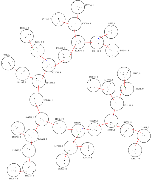
Figure 12. A chirotope tree of 36 nodes, each decorated with a chirotope of size $9$, adding up to $254$ elements. The numbers next to each node indicate the identifier of the decorating chirotope in the order type database [AAK02] and the label of the red proxy in this database.

9.3. A proof-of-concept implementation

We implemented the method described in the previous section (both the modification of the Alvarez-Seidel algorithm and the recursive counting behind Proposition 1.4) for the special case of trees where

• every node has degree at most $3$,

• every node of arity $3$ is decorated by a chirotope with only $3$ extreme elements, which are its proxies, and

• every node of arity $2$ has its two proxies consecutive on the convex hull.

These conditions ensure that in any triangulation of a chirotope decorating a node of $T$, there is always an edge between any two proxies. This allows to omit the variables $y_{i,j}$ introduced in Definition 9.1. We propose it as a proof of concept: we made little effort in optimizing or benchmarking it as either is beyond the scope of this paper.

9.3.1. Repository

Our implementation runs within Sagemath to take advantage of basic functions for the manipulation of multivariate polynomials, but is mostly basic python. The code in Sagemath can be found on the repository chirotope_tree. The example of Figure 12 can be obtained by running the command sage -python example.py, which prints two numbers, first the number of triangulation of the example, and the total time spent in seconds on computing it (ignoring the initial time to launch sage).

9.3.2. An example

Our code computes in a few seconds on a standard laptop that the number of triangulations of the chirotope of size $254$ presented by the tree of Figure 12 is

$$59 2\,966\,751\,293\,974\,711\,252\,579\,414\,478\,724\,131\,868\,483\,318\,559\,312\,640\,993\,804\,562\,350\,446$$

$$478\,462\,502\,194\,102\,338\,465\,347\,793\,563\,468\,964\,711\,887\,069\,260\,192\,677\,783\,5079\,385\,675$$

$$578\,362\,313\,461\,572\,573\,372\,584\,158\,103\,703\,847\,713\,232\,664\approx 5.92966751.10^{180}$$

References

- [AA05] M. H. Albert and M. D. Atkinson. Simple permutations and pattern restricted permutations. Discrete Mathematics, 300(1-3):1–15, 2005.
- [AAK02] O. Aichholzer, F. Aurenhammer, and H. Krasser. Enumerating order types for small point sets with applications. Order, 19(3):265–281, 2002.
- [AEG+94] B. Aronov, P. Erdős, W. Goddard, D. J. Kleitman, M. Klugerman, J. Pach, and L. J. Schulman. Crossing families. Combinatorica, 14(2):127–134, 1994.
- [AS13] V. Alvarez and R. Seidel. A simple aggregative algorithm for counting triangulations of planar point sets and related problems. In Proceedings of the twenty-ninth annual symposium on Computational geometry, pages 1–8, 2013.
- [BBF+22] F. Bassino, M. Bouvel, V. Féray, L. Gerin, M. Maazoun, and A. Pierrot. Random cographs: Brownian graphon limit and asymptotic degree distribution. Random Struct. Algorithms, 60(2):166–200, 2022.
- [BBR11] F. Bassino, M. Bouvel, and D. Rossin. Enumeration of pin-permutations. Electronic Journal of Combinatorics, 18, 2011.
- [BFG+02] C. Banderier, P. Flajolet, D. Gardy, M. Bousquet-Mélou, A. Denise, and D. Gouyou-Beauchamps. Generating functions for generating trees. Discrete Mathematics, 246(1–3):29–55, 2002.
- [BLVS+99] A. Björner, M. Las Vergnas, B. Sturmfels, N. White, and G. M. Ziegler. Oriented matroids. Number 46 in Encyclopedia of Mathematics and its Applications. Cambridge University Press, 1999.
- [CFL17] C. Chauve, E. Fusy, and J. Lumbroso. An exact enumeration of distance-hereditary graphs. In 2017 Proceedings of the Fourteenth Workshop on Analytic Algorithmics and Combinatorics (ANALCO’17), pages 31–45, 2017.
- [EVDHM22] J. Erickson, I. Van Der Hoog, and T. Miltzow. Smoothing the gap between NP and ER. SIAM Journal on Computing, 51(2):FOCS20–102–138, 2022.
- [FG17] S. Felsner and J. E. Goodman. Pseudoline arrangements. In Handbook of Discrete and Computational Geometry, pages 125–157. Chapman and Hall/CRC, 2017.
- [Gal67] T. Gallai. Transitiv orientierbare Graphen. Acta Mathematica Academiae Scientiarum Hungarica, 18(1–2):25–66, March 1967.
- [GP83] J. E. Goodman and R. Pollack. Multidimensional sorting. SIAM J. Comput., 12(3):484–507, 1983.
- [GP93] J. E. Goodman and R. Pollack. Allowable sequences and order types in discrete and computational geometry. In New trends in discrete and computational geometry, pages 103–134. Berlin: Springer-Verlag, 1993.
- [GW23] X. Goaoc and E. Welzl. Convex hulls of random order types. Journal of the ACM, 70(1):Article No. 8: 1–47, 2023.
- [HP10] M. Habib and C. Paul. A survey of the algorithmic aspects of modular decomposition. Computer Science Review, 4(1):42–59, February 2010.
- [MM16] D. Marx and T. Miltzow. Peeling and Nibbling the Cactus: Subexponential-Time Algorithms for Counting Triangulations and Related Problems. In S. Fekete and A. Lubiw, editors, 32nd International Symposium on Computational Geometry (SoCG 2016), volume 51 of Leibniz International Proceedings in Informatics (LIPIcs), pages 52:1–52:16, Dagstuhl, Germany, 2016. Schloss Dagstuhl – Leibniz-Zentrum für Informatik.
- [MR84] R. H. Möhring and F. J. Radermacher. Substitution decomposition for discrete structures and connections with combinatorial optimization. Annals of Discrete Math, 19:257–356, 1984.
- [Rao08] M. Rao. Solving some NP-complete problems using split decomposition. Discrete Appl. Math., 156(14):2768–2780, 2008.
- [RG11] J. Richter-Gebert. Perspectives on projective geometry: a guided tour through real and complex geometry. Springer, 2011.
- [RW23] D. Rutschmann and M. Wettstein. Chains, Koch chains, and point sets with many triangulations. Journal of the ACM, 70(3):1–26, 2023.
- [Sam88] P. Samuel. Projective geometry. Springer, 1988.
- [Sha11] A. Sharir, Micha Sheffer. Counting triangulations of planar point sets. The Electronic Journal on Combinatorics, 18(1):1–70, 2011.
- [Sho91] P. Shor. Stretchability of pseudolines is NP-hard. Applied Geometry and Discrete Mathematics-The Victor Klee Festschrift, 1991.
- [SY17] V. Sharma and C. K. Yap. Robust geometric computation. In Handbook of Discrete and Computational Geometry, pages 1189–1223. Chapman and Hall/CRC, 2017.
- [SZ23] A. Suk and J. Zeng. A positive fraction Erdős–Szekeres theorem and its applications. Discrete & Computational Geometry, pages 1–18, 2023.
- [Val97] P. Valtr. On mutually avoiding sets. In The Mathematics of Paul Erdös II, pages 324–328. Springer, 1997.
- [War68] H. E. Warren. Lower bounds for approximation by nonlinear manifolds. Transactions of the American Mathematical Society, 133(1):167–178, 1968.
- [Zas97] T. Zaslavsky. Facing up to arrangements: face-count formulas for partitions of space by hyperplanes. Memoirs of American Mathematical Society, 154:1–95, 1997.