Low-energy theorems for neutron-proton scattering in $\chi$EFT using a perturbative power counting

Abstract

Low-energy theorems (LETs) for effective-range parameters in nucleon-nucleon scattering encode properties of the long-range part of the nuclear force. We compute LETs for S-wave neutron-proton scattering using chiral effective field theory ($\chi$EFT) with a modified version of Weinberg power counting. Corrections to the leading order amplitude are included in distorted-wave perturbation theory and we include contributions up to the third order in the power counting. We find that LETs in the ${}^{3}S_{1}$ partial wave agree excellently with the empirical effective-range parameters while LETs in the ${}^{1}S_{0}$ partial wave show a fairly good agreement. At the same time, phase shifts up to laboratory scattering energies of about 100 MeV can be reproduced. The contributions from two-pion exchange do not improve the LETs in the ${}^{1}S_{0}$ partial wave, and a noticeable dependence on the employed momentum space cutoff emerges in the ${}^{3}S_{1}$ partial wave for cutoffs smaller than 750 MeV. The results show that empirical effective-range parameters and phase shifts can be reproduced simultaneously in the employed power counting and that LETs might be useful when inferring low-energy constants in power countings where corrections are added perturbatively.

1 Introduction

The importance of the low-energy limit in quantum mechanical scattering dates back to the work of H. Bethe Bethe:1949yr , who realized that two-particle scattering at sufficiently low energies possesses a universal behavior characterized by only two parameters: the scattering length and effective range. This universal theory was extended to what is known as effective range theory by utilizing analytical properties of the scattering amplitude. Besides successfully parameterizing low-energy scattering amplitudes, effective range theory can serve as a tool to analyze the low-energy properties of nuclear interaction models derived from effective field theories (EFTs) Cohen:1998jr .

In seminal works Weinberg:1990rz ; Weinberg:1991um , Weinberg proposed to apply an EFT description to model the nuclear force based on the spontaneously broken chiral symmetry of low-energy Quantum Chromodynamics (QCD). In this EFT, pion-nucleon interactions are governed by a Lagrangian consistent with the low-energy symmetries of QCD. Nuclear interaction potentials can be constructed by assessing the relative importance of the emerging effective interactions in what is known as power counting (PC) Epelbaum:2008ga ; Machleidt:2011zz ; Hammer:2019poc . The PC is performed in terms of $(Q/\Lambda_{b})^{\nu}$, where $Q$ denotes the relevant low-energy scales and $\Lambda_{b}$ the breakdown scale of the EFT. In nucleon-nucleon ($NN$) scattering $Q\sim\{p,m_{\pi}\}$, where $p$ is the modulus of the $NN$ relative momentum and $m_{\pi}$ the average pion mass. We refer to $\nu$ as the chiral order, and specifically $\nu=0$ as leading order (LO), $\nu=1$ as next-to-leading order (NLO), and so on. The resulting EFT, known as chiral effective field theory ($\chi$EFT), has been employed in the last decades to develop two- and three-nucleon potentials to high chiral orders Ordonez:1995rz ; vanKolck:1994yi ; Ordonez:1993tn ; Entem:2015xwa ; Reinert:2017usi ; Epelbaum:2002vt . Low-energy constants (LECs) parametrize the unknown coupling strengths in the Lagrangian, and thus appear in the potentials, and need to be inferred from data. The $\chi$EFT potentials in combination with computational advancements in solving the many-body Schrödinger equation have enabled quantitative EFT predictions of nuclear properties across the nuclear chart, see e.g. Refs Hagen:2015yea ; Arthuis:2020toz ; Hu:2021trw .

To date, Weinberg PC (WPC) is the main PC being used to construct quantitative chiral potentials. However, an ongoing effort to construct alternative PCs has been pursued to construct renormalization-group (RG) invariant interactions. The amplitudes in WPC are not RG-invariant in the sense that the momentum space cutoff used to regulate the divergences cannot be taken arbitrarily large. This can be traced to the non-perturbative treatment of singular potentials, which leads to uncontrolled divergences if sufficient counterterms are not included Nogga:2005hy ; vanKolck:2020llt ; Long:2007vp ; PhysRevA.64.042103 (see, e.g., Ref. Epelbaum:2018zli for another approach to deal with the singular interactions in $\chi$EFT). In the late 1990s, Kaplan et al. Kaplan:1998tg ; Kaplan:1998we proposed an RG-invariant PC where pions are treated perturbatively in all $NN$ partial waves. Despite some success in describing scattering phase shifts, further studies showed that the convergence radius in terms of scattering energy was not improved compared to a theory without pions Fleming:1999ee .

Cohen and Hansen Cohen:1998jr ; Cohen:1999iaa further investigated this PC (often referred to as KSW counting) by studying the $S$-wave effective range expansion (ERE) for the neutron-proton ($np$) scattering amplitude. They showed that the higher-order ERE parameters beyond the scattering length and effective range are predicted functions of the scattering length, nucleon mass, and the parameters defining the long-range pion-exchange potential. By calibrating the unknown LECs to reproduce the empirical scattering length and effective range, the higher-order ERE parameters are thus predictions solely governed by the long-range part of the interaction. We will refer to such predictions of ERE parameters as low-energy theorems (LETs) Cohen:1998jr ; Cohen:1999iaa . Cohen and Hansen compared the LETs with empirical ERE parameters extracted from the Nijmegen partial wave analysis Stoks:1993tb , where the latter provides a robust parametrization of the low-energy behavior of the nuclear force NavarroPerez:2014ovp . The comparison showed a poor agreement between the LETs and the empirical ERE parameters while the PC produces realistic phase shifts Kaplan:1998tg ; Kaplan:1998we . The main conclusion of Refs. Cohen:1998jr ; Cohen:1999iaa was that LETs serve as a non-trivial test to identify if the long-range part of the potential induces a correct near-threshold energy dependence of the scattering amplitude.

Following Ref. Cohen:1998jr , LETs have been used as a tool to study the low-energy properties of EFT potentials Ando:2011aa ; PavonValderrama:2003np ; Epelbaum:2004fk and Ref. Epelbaum:2003xx showed that LETs computed in WPC has a good agreement with empirical ERE parameters extracted in Ref. Stoks:1993tb . Furthermore, in Epelbaum:2009sd LETs are used as a tool to study renormalization problems; and Refs. Baru:2015ira ; Baru:2016evv derive low-energy theorems for a varying pion mass and apply them to analyze lattice-QCD calculations.

In this paper, we study LETs for $np$ scattering in $S$-waves up to next-to-next-to-next-to-leading order (N³LO) applying the perturbative and RG-invariant modified WPC (MWPC) proposed by Long and Yang Long:2012ve ; PhysRevC.84.057001 ; PhysRevC.85.034002 . It has been demonstrated that phase shifts, $np$ scattering observables and binding energies in $A=3,4$ nuclei can be described in the Long and Yang PC Long:2012ve ; PhysRevC.84.057001 ; PhysRevC.85.034002 ; Thim:2023fnl ; Thim:2024yks ; Yang:2020pgi , but LETs have not been investigated. We want to study LETs to quantify the accuracy to which pion exchanges describe the low-energy part of the two-nucleon interaction in this PC. We specifically study if the MWPC LETs and phase shifts can describe their empirical counterparts simultaneously—since both are essential for a theoretically sound PC with an ambition to quantitatively describe the nuclear force. The Long and Yang PC differs from WPC in the ${}^{1}S_{0}$ partial wave by having promoted contact interactions and by treating sub-leading ($\nu>0$) interactions perturbatively. Ref. Baru:2015ira emphasizes that two-pion exchange contributions are expected to be important for describing LETs in the ${}^{1}S_{0}$ partial wave and it is unknown if this can be achieved with a perturbative inclusion. In the ${}^{3}S_{1}\mathrm{-}^{3}D_{1}$ channel the only difference compared to WPC is that sub-leading interactions are treated perturbatively, meaning that our study in this channel specifically targets the feasibility of including two-pion exchange contributions perturbatively. Importantly, the EFT truncation error stemming from the truncated chiral expansion Ekstrom:2013kea ; Schindler:2008fh ; Furnstahl:2014xsa is not taken into account in this study, the uncertainty in the predictions is instead estimated using the residual cutoff dependence Griesshammer:2015osb .

The article is organized as follows. Section 2 contains a brief overview of how $np$ scattering amplitudes are computed in the Long and Yang PC. In Section 3, LETs are computed in the ${}^{1}S_{0}$ and ${}^{3}S_{1}$ partial waves at orders LO to N³LO and compared to similar studies Cohen:1998jr ; Cohen:1999iaa ; Ando:2011aa ; Epelbaum:2003xx ; Epelbaum:2012ua ; Epelbaum:2015sha . Finally, in Section 4 we conclude and discuss prospects for future analyses carefully accounting for the EFT error and its effect on the predicted LETs.

2 Computing scattering amplitudes and phase shifts

This section contains a brief summary of how $np$ scattering amplitudes are computed in $\chi$EFT using the Long and Yang PC developed in Refs. Long:2012ve ; PhysRevC.84.057001 ; PhysRevC.85.034002 . We consider a scattering process of an incoming neutron with kinetic energy $T_{\mathrm{lab}}$ impinging on a proton. Specifically, we only investigate the two $S$-wave channels: ${}^{1}S_{0}$ and ${}^{3}S_{1}\mathrm{-}^{3}D_{1}$. In $\chi$EFT, the $np$ potential gets contributions from both contact interactions of zero range and finite range interactions generated by pion exchanges. The potential contributions in the Long and Yang PC are organized in chiral orders as Long:2012ve ; PhysRevC.84.057001 ; PhysRevC.85.034002

$$\mathrm{LO:} V^{(0)}=V^{(0)}_{1\pi}+V^{(0)}_{\mathrm{ct}}$$ (1)

$$\mathrm{NLO:} V^{(1)}=V^{(1)}_{\mathrm{ct}}$$

$$\mathrm{N}^{2}\mathrm{LO:} V^{(2)}=V^{(2)}_{2\pi}+V^{(2)}_{\mathrm{ct}}$$

$$\mathrm{N}^{3}\mathrm{LO:}\ V^{(3)}=V^{(3)}_{2\pi}+V^{(3)}_{\mathrm{ct}}$$

where $V^{(\nu)}_{1\pi}$, $V^{(\nu)}_{2\pi}$ and $V^{(\nu)}_{\mathrm{ct}}$ denote one-pion exchange, two-pion exchange, and contact potentials respectively. The contact potentials are parameterized by LECs which need to be fixed using experimental data. For further details about the PC, we refer to Refs. Long:2012ve ; PhysRevC.84.057001 ; PhysRevC.85.034002 ; Thim:2024yks .

The one-pion exchange potential enters at LO in the considered channels and reads Machleidt:2011zz

$$V^{(0)}_{1\pi}=-\frac{g^{2}_{A}}{4f^{2}_{\pi}}\frac{\left(\bm{\sigma}_{1}\cdot\bm{q}\right)\left(\bm{\sigma}_{2}\cdot\bm{q}\right)}{\bm{q}^{2}+m^{2}_{\pi}}\left(\bm{\tau}_{1}\cdot\bm{\tau}_{2}\right)$$ (2)

where $\bm{\tau}_{i}$ and $\bm{\sigma}_{i}$, for $i=1,2$, denote the isospin and spin operators for the respective nucleon, $\bm{p}$ ($\bm{p}^{\prime}$) the ingoing (outgoing) relative $np$-momentum and $\bm{q}=\bm{p}^{\prime}-\bm{p}$ the momentum transfer. The numerical values employed for the constants are: pion-nucleon axial coupling $g_{A}=1.29$, average pion mass $m_{\pi}=138.039$ MeV, and pion decay constant $f_{\pi}=92.1$ MeV. The LO contact potential has contributions in the ${}^{1}S_{0}$ and ${}^{3}S_{1}\mathrm{-}^{3}D_{1}$ channels which are given by

$$V^{(0)}_{\mathrm{ct}}=C^{(0)}_{{}^{1}S_{0}}\hat{P}_{{}^{1}S_{0}}+C^{(0)}_{{}^{3}S_{1}}\hat{P}_{{}^{3}S_{1}},$$ (3)

where $\hat{P}_{X}$ denotes the projector onto the given partial wave and the constants $C^{(0)}_{X}$ denote the LO LECs. The superscript indicates that these are the first contributions to the LECs: $C_{{}^{1}S_{0}}$ and $C_{{}^{3}S_{1}}$ which also receive contributions at sub-leading orders since the higher order potentials are added perturbatively Long:2012ve ; Contessi:2017rww . For the two-pion exchange, we use expressions computed using dimensional regularization Machleidt:2011zz and for the sub-leading two-pion exchange ($V^{(3)}_{2\pi}$) we employ $c_{i}$ LECs: $c_{1}=-0.74$ GeV^-1, $c_{3}=-3.61$ GeV^-1 and $c_{4}=2.44$ GeV^-1 from the Roy-Steiner analysis of pion-nucleon scattering amplitudes presented in Ref. Siemens:2016jwj . Explicit expressions for all potentials are documented in the Appendix of Ref. Thim:2024yks .

The $np$ scattering amplitude at order $\nu$ is denoted $T^{(\nu)}$, analogous to the notation for the potentials. The LO amplitude is computed non-perturbatively by solving the Lippmann–Schwinger equation with the LO potential

$$T^{(0)}=V^{(0)}+V^{(0)}G^{+}_{0}T^{(0)},$$ (4)

where $G^{+}_{0}=\left(E-H_{0}+i\epsilon\right)^{-1}$ is the free resolvent, $H_{0}=\bm{p}^{2}/m_{N}$ the free Hamiltonian, $m_{N}$ the nucleon mass and $E=k^{2}/m_{N}$ the center-of-mass energy corresponding relative momentum $k$. Sub-leading corrections to the scattering amplitude are computed using distorted wave perturbation theory Long:2007vp ; Peng:2020nyz using the equations Thim:2024yks

$$T^{(1)} =\Omega^{\dagger}_{-}V^{(1)}\Omega_{+}$$ (5)

$$T^{(2)} =\Omega^{\dagger}_{-}\left(V^{(2)}+V^{(1)}G^{+}_{1}V^{(1)}\right)\Omega_{+}$$ (6)

$$T^{(3)} =\Omega^{\dagger}_{-}\Big{(}V^{(3)}+V^{(2)}G^{+}_{1}V^{(1)}+V^{(1)}G^{+}_{1}V^{(2)}+$$

$$+V^{(1)}G^{+}_{1}V^{(1)}G^{+}_{1}V^{(1)}\Big{)}\Omega_{+},$$ (7)

where we have introduced the operators $\Omega_{+}=\mathds{1}+G^{+}_{0}T^{(0)}$, $\Omega^{\dagger}_{-}=\mathds{1}+T^{(0)}G^{+}_{0}$ and $G^{+}_{1}=\Omega_{+}G^{+}_{0}$. The partial wave scattering amplitudes are computed numerically using matrix discretization Haftel:1970zz by expressing Eqs. 4, 5, 6 and 7 in a partial wave basis $\ket{p,\ell sj}$. Here, $p=\absolutevalue{\bm{p}}$, and $\ell$, $s$, $j$ are the quantum numbers associated with the $np$ orbital angular momentum, spin, and total angular momentum, respectively. The partial-wave Lippmann–Schwinger equation reads

$$T^{(0)sj}_{\ell^{\prime}\ell}(p^{\prime},p)=V^{(0)sj}_{\ell^{\prime}\ell}(p^{\prime},p)+\sum_{\ell^{\prime\prime}}\int_{0}^{\infty}dq\ q^{2}V^{(0)sj}_{\ell^{\prime}\ell^{\prime\prime}}(p^{\prime},q)\frac{m_{N}}{k^{2}-q^{2}+i\epsilon}T^{(0)sj}_{\ell^{\prime\prime}\ell}(q,p),$$ (8)

where $k=\sqrt{m_{N}E}$ denote the on-shell relative momentum corresponding to $T_{\mathrm{lab}}$ Glockle . The notation $T^{(\nu)sj}_{\ell^{\prime}\ell}(p^{\prime},p)\equiv\bra{p^{\prime},\ell^{\prime}sj}T^{(\nu)}\ket{p,\ell sj}$ is used for amplitudes and potentials. The partial wave projected potentials are regulated using the transformation

$$V^{(\nu)sj}_{\ell^{\prime}\ell}(p^{\prime},p)\to\exp\left(-\frac{p^{\prime 6}}{\Lambda^{6}}\right)V^{(\nu)sj}_{\ell^{\prime}\ell}(p^{\prime},p)\exp\left(-\frac{p^{6}}{\Lambda^{6}}\right)$$ (9)

where $\Lambda$ is referred to as the momentum cutoff.

The contributions to the scattering amplitude at each order, $T^{(\nu)sj}_{\ell^{\prime}\ell}$, can now be computed for $\nu\leq 3$ in each scattering channel. The total on-shell amplitude ($p^{\prime}=p=k$) is obtained by summing the contributions to the desired order according to

$$T^{sj}_{\ell^{\prime}\ell}(k,k)=T^{(0)sj}_{\ell^{\prime}\ell}(k,k)+T^{(1)sj}_{\ell^{\prime}\ell}(k,k)+T^{(2)sj}_{\ell^{\prime}\ell}(k,k)+\dots$$ (10)

Using the relation between the scattering amplitude and $S$-matrix,

$$S^{sj}_{\ell^{\prime}\ell}=\delta_{\ell^{\prime}\ell}-i\pi km_{N}T^{sj}_{\ell^{\prime}\ell},$$ (11)

phase shift contributions can be computed at each chiral order by expanding Eq. 11 and matching chiral orders. This is described in Appendix B and yields expansions for the corresponding shifts in chiral orders analogous to Eq. 10

$$\delta(k)=\delta^{(0)}(k)+\delta^{(1)}(k)+\delta^{(2)}(k)+\dots$$ (12)

In the next section, the scattering amplitudes are utilized to compute both phase shifts and LETs.

3 Low-energy theorems for effective range parameters

The $S$-wave effective range function, $F(k)$, can be expressed in terms of the $S$-wave phase shift, $\delta(k)$, and possesses the property of being analytic in $k^{2}$ near the origin giving the ERE

$$F(k)\equiv k\cot{\delta}\left(k\right)=-\frac{1}{a}+\frac{1}{2}rk^{2}+v_{2}k^{4}+v_{3}k^{6}+v_{4}k^{8}+\mathcal{O}\left(k^{10}\right).$$ (13)

The ERE parameters $a$ and $r$ are called the scattering length and effective range, while $v_{2},v_{3}$ and $v_{4}$ are referred to as shape parameters. The presence of pions in $\chi$EFT restricts the radius of convergence for the ERE to $k<m_{\pi}/2\approx 69$ MeV corresponding to the first left-hand singularity in the scattering amplitude caused by one-pion exchange Baru:2015ira . Hence, the ERE converges for $T_{\mathrm{lab}}\lesssim 10$ MeV, in what is referred to as the low-energy regime.

To compute LETs, the unknown LECs must first be inferred from either phase shifts Stoks:1993tb , the first few empirical effective range parameters, or a mix of both. The effective range function in Eq. 13 can then be computed, and the remaining ERE parameters not used to calibrate the LECs are predictions governed by the long-range part of the interaction (LETs) Cohen:1998jr . In the coming sections, we will compute LETs in the ${}^{1}S_{0}$ and ${}^{3}S_{1}$ partial waves where the scattering amplitudes and the effective range function are computed perturbatively beyond LO.

3.1 The ${}^{1}S_{0}$ partial wave

We first consider the ${}^{1}S_{0}$ partial wave and thus suppress its associated quantum numbers from the notation. For uncoupled $np$ scattering channels, it is convenient to express the effective range function directly in terms of the on-shell scattering amplitude, $T(k,k)$, using the relation Taylor72

$$T(k,k)=-\frac{2}{\pi m_{N}}\frac{1}{F(k)-ik}.$$ (14)

By treating sub-leading amplitudes as perturbations to $T^{(0)}$, Taylor expanding Eq. 14 and keeping terms to order $\nu=3$ one obtains

$$F(k)-ik =-\frac{2}{\pi m_{N}T^{(0)}}\Bigg{[}1-\frac{T^{(1)}}{T^{(0)}}+\left(\left[\frac{T^{(1)}}{T^{(0)}}\right]^{2}-\frac{T^{(2)}}{T^{(0)}}\right)+$$

$$+\left(2\frac{T^{(1)}T^{(2)}}{\big{(}T^{(0)}\big{)}^{2}}-\frac{T^{(3)}}{T^{(0)}}-\left[\frac{T^{(1)}}{T^{(0)}}\right]^{3}\right)+\mathcal{O}\left(\frac{Q^{4}}{\Lambda^{4}_{b}}\right)\Bigg{]}.$$ (15)

The effective range function can be written in terms of contributions at each chiral order, analogous to the scattering amplitude

$$F(k)=F^{(0)}(k)+F^{(1)}(k)+F^{(2)}(k)+\dots$$ (16)

These contributions are identified in Eq. 15 and read

$$F^{(0)}(k) =-\frac{2}{\pi m_{N}T^{(0)}}+ik$$ (17)

$$F^{(1)}(k) =\frac{2}{\pi m_{N}T^{(0)}}\frac{T^{(1)}}{T^{(0)}}$$ (18)

$$F^{(2)}(k) =-\frac{2}{\pi m_{N}T^{(0)}}\left(\left[\frac{T^{(1)}}{T^{(0)}}\right]^{2}-\frac{T^{(2)}}{T^{(0)}}\right)$$ (19)

$$F^{(3)}(k) =-\frac{2}{\pi m_{N}T^{(0)}}\left(2\frac{T^{(1)}T^{(2)}}{\big{(}T^{(0)}\big{)}^{2}}-\frac{T^{(3)}}{T^{(0)}}-\left[\frac{T^{(1)}}{T^{(0)}}\right]^{3}\right).$$ (20)

Note that in a theory without pions, the renormalized LO amplitude possesses the property that $\mathrm{Re}\big{\{}\left(T^{(0)}\right)^{-1}\big{\}}$ is a momentum independent constant and all coefficients but $a$ in the ERE will be zero by Eq. 17. This illustrates the fact that non-zero ERE parameters beyond $a$ at LO can be attributed to the presence of a long-range force, in our case the one-pion exchange.

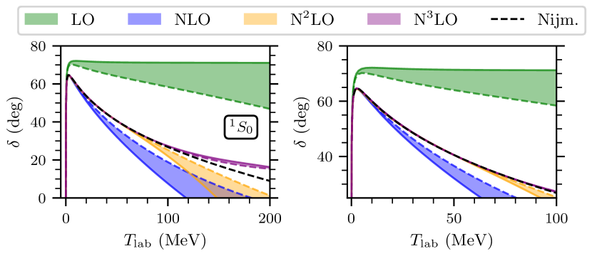
Figure 1: Phase shifts in the ${}^{1}S_{0}$ partial wave as a function of laboratory scattering energy for the LEC calibration with corresponding ERE parameters in Table 1. The bands indicate the envelope of the variation due to the two different cutoff values; 500 MeV (dashed line) and 2500 MeV (solid line). The black dashed line shows phase shifts from the Nijmegen analysis Stoks:1993tb . The right panel shows the same phase shifts but for a reduced energy interval.

Table 1: LETs for the ${}^{1}S_{0}$ partial wave. The ERE parameters marked with a star ($*$) are used in the inference and are not predictions. The quoted errors only stem from the numerical extraction of the ERE parameters from the perturbatively computed effective range function. Empirical ERE parameters are also shown.

${}^{1}S_{0}$ partial wave	$a$ [fm]	$r$ [fm]	$v_{2}$ [fm3]	$v_{3}$ [fm5]	$v_{4}$ [fm7]
Empirical (Ref. NavarroPerez:2014ovp )	$-23.735(16)$	2.68(3)	$-0.48(2)$	3.9(1)	$-19.6(5)$
$\Lambda=500$ MeV
LO	$*$	$1.71(0)$	$-1.77(0)$	$8.54(0)$	$-47.0(3)$
NLO	$*$	$*$	$-0.64(0)$	$4.79(0)$	$-29.9(2)$
N2LO	$*$	$2.72(0)$	$-0.71(0)$	$5.05(0)$	$-29.3(2)$
N3LO	$*$	$2.69(0)$	$-0.66(0)$	$5.42(0)$	$-31.0(2)$
$\Lambda=2500$ MeV
LO	$*$	$1.49(0)$	$-2.06(0)$	$9.34(0)$	$-50.7(3)$
NLO	$*$	$*$	$-0.55(0)$	$4.70(0)$	$-30.1(2)$
N2LO	$*$	$2.75(0)$	$-0.75(0)$	$4.80(0)$	$-28.1(2)$
N3LO	$*$	$2.70(0)$	$-0.69(0)$	$5.52(0)$	$-30.6(5)$

To compute phase shifts and LETs, the unknown LECs first need to be inferred. In this study, we neglect both the truncation error associated with the $\chi$EFT expansion and the uncertainties associated with the calibration data during the inference, similar to earlier studies Cohen:1998jr ; Cohen:1999iaa ; Epelbaum:2012ua ; Epelbaum:2015sha . Instead, we utilize that adding higher chiral orders improves the high-energy description. Consequently, we successively include higher-energy data in the calibration as the chiral order is increased. A measure of the theoretical uncertainty is provided by doing the calculations using different momentum cutoffs $\Lambda=500$ MeV and $\Lambda=2500$ MeV, where the residual cutoff dependence is expected to indicate the effect of excluded terms in the chiral expansion Griesshammer:2015osb .

We wish to obtain LETs that describe empirical ERE parameters while the predicted phase shifts show a good description of their empirical counterparts. To achieve this, we employ both empirical phase shifts and ERE parameters as data to calibrate the LECs, where the latter are shown in the first row of Table 1 NavarroPerez:2014ovp . The LEC at LO, $C^{(0)}_{{}^{1}S_{0}}$, is calibrated to reproduce the scattering length. The two LECs at NLO are calibrated to reproduce both $a$ and $r$. At N²LO the three LECs are calibrated using $a$, as well as the Nijmegen phase shifts Stoks:1993tb at $T_{\mathrm{lab}}=25$ MeV and 50 MeV. At N³LO the four LECs are inferred from $a$ as well as the Nijmegen phase shifts at $T_{\mathrm{lab}}=5$ MeV, 50 MeV, and $75$ MeV. LETs are computed by performing a least squares fit of the ERE polynomial (Eq. 13) to the effective range function computed to the desired order: $F^{(0)}(k)$ at LO, $F^{(0)}(k)+F^{(1)}(k)$ at NLO and so on.

The resulting phase shifts and LETs are presented in Fig. 1 and Table 1, respectively. The phase shifts show a clear order-by-order convergence, and at N³LO it agrees excellently with the Nijmegen phase shift up to $T_{\mathrm{lab}}\approx 100$ MeV, as highlighted in the right panel of Fig. 1. The cutoff variation in both phase shifts and LETs decreases as the chiral order increases, according to qualitative expectations. The uncertainties presented in the LETs only stem from the numerical extraction of the ERE parameters and are estimated by varying both momentum interval and polynomial order used in the least squares fit. It can be seen that these errors are negligible for all ERE parameters except $v_{4}$.

The obtained LETs for LO and NLO are consistent with similar studies Epelbaum:2012ua ; Epelbaum:2015sha , whose results are summarized in Table 4 in Appendix A. The computed LETs improve going from LO to NLO, i.e. when including the contact interaction $D^{(0)}_{{}^{1}S_{0}}\left(p^{2}+p^{\prime 2}\right)$ Long:2012ve ; Thim:2024yks . No further improvements are observed at N²LO and N³LO when the leading- and sub-leading two pion exchanges are included. Thus, convergence to the empirical values of the ERE parameters is not observed as the chiral order is increased. Even though the LETs for the shape parameters: $v_{2},v_{3}$ and $v_{4}$ perform worse compared to the ones obtained in WPC Epelbaum:2003xx , they are significantly improved compared to KSW counting Kaplan:1998tg ; Kaplan:1998we ; Cohen:1998jr , see Table 4. It should be emphasized that a perturbative calculation of scattering amplitudes and LETs is significantly different from non-perturbatively solving the Lippmann–Schwinger equation, where the latter method is applied for both WPC and the high-precision potentials. It is not clear if, or how, this difference impacts how LETs should be interpreted and compared.

Let us now explore the effects of employing an alternate scheme to infer the LECs, to gauge how the choice of calibration data impacts the results. First, we investigate the effect of only using effective range parameters to calibrate the LECs. In this calculation we employ the cutoff $\Lambda=500$ MeV. We calibrate the LECs to reproduce $\{a\}$, $\{a,r\}$ and $\{a,r,v_{2}\}$ for LO to N²LO respectively. At N³LO there is one additional LEC compared to N²LO, and $v_{3}$ can be included in the calibration data. However, we find no set of LECs that can reproduce $\{a,r,v_{2},v_{3}\}$ simultaneously. We find, however, that it is possible by slightly adjusting the values of some empirical ERE parameters, which hints at the fact that accounting for uncertainties can resolve this apparent issue. At N³LO the LECs are instead calibrated to $a$, and the phase shifts at $T_{\mathrm{lab}}=5,50$ and $75$ MeV.

The resulting phase shifts and LETs are shown in the left panel of Fig. 2 and Table 2, respectively. It is observed that the obtained phase shifts and LETs at N²LO perform worse than the ones at NLO. The N²LO LETs are also performing worse than the ones presented in Table 1. It can be concluded that including $v_{2}$ in the calibration data at N²LO is not beneficial for either phase shifts nor LETs. At N³LO, it is shown that it is possible to obtain realistic phase shifts at N³LO also in this alternative calibration scheme while getting LETs comparable to the results in Table 1. The same calibration was tried with $\Lambda=2500$ MeV but it was not possible to simultaneously reproduce $\{a,r,v_{2}\}$ at N²LO. One potential explanation is that the LO phase shift for $\Lambda=2500$ MeV exhibits a greater overestimation of the Nijmegen phase shift compared to the $\Lambda=500$ MeV phase shift (see Fig. 1), thus necessitating a larger correction from the sub-leading orders. Compared to the first calibration, it can be concluded that inferring LECs solely using ERE parameters does not seem to be beneficial. Including phase shifts in the calibration data can thus be interpreted as having a regulating effect and mitigating the possible overfitting to ERE parameters. This regulating effect will now be investigated further.

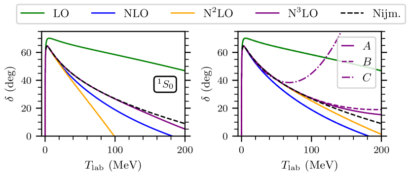
Figure 2: Phase shifts in the ${}^{1}S_{0}$ partial wave for $\Lambda=500$ MeV. The left panel shows the predicted phase shifts from calibrating the LECs using the data $\{a\}$, $\{a,r\}$, $\{a,r,v_{2}\}$, $\{a,\delta_{5},\delta_{50},\delta_{75}\}$ for orders LO to N³LO respectively. Here, $\delta_{X}$ denotes the ${}^{1}S_{0}$ phase shift from the Nijmegen analysis Stoks:1993tb at $T_{\mathrm{lab}}=X$ MeV. In the right panel, the calibration at LO to N²LO is done like in Fig. 1. At N³LO, the solid, dashed and dot-dashed lines correspond to using the calibration data $A=\{a,\delta_{5},\delta_{50},\delta_{75}\}$, $B=\{a,r,\delta_{50},\delta_{75}\}$ and $C=\{a,r,v_{2},\delta_{50}\}$ respectively.

Table 2: LETs for $\Lambda=500$ MeV corresponding to the phase shifts presented in Fig. 2. The parameters marked with a star ($*$) are used in the inference and are not predictions. The quoted errors only stem from the numerical extraction of the ERE parameters from the perturbatively computed effective range function. Empirical ERE parameters are also shown.

${}^{1}S_{0}$ partial wave	$a$ [fm]	$r$ [fm]	$v_{2}$ [fm3]	$v_{3}$ [fm5]	$v_{4}$ [fm7]
Empirical (Ref. NavarroPerez:2014ovp )	$-23.735(16)$	2.68(3)	$-0.48(2)$	3.9(1)	$-19.6(5)$
(left panel Fig. 2)
LO	$*$	$1.71(0)$	$-1.77(0)$	$8.54(0)$	$-47.0(3)$
NLO	$*$	$*$	$-0.64(0)$	$4.79(0)$	$-29.9(2)$
N2LO	$*$	$*$	$*$	$5.89(0)$	$-32.3(2)$
N3LO	$*$	$2.69(0)$	$-0.61(0)$	$5.51(0)$	$-30.9(2)$
(right panel Fig. 2)
N3LO ($A$)	$*$	$2.69(0)$	$-0.66(0)$	$5.42(0)$	$-31.0(2)$
N3LO ($B$)	$*$	$*$	$-0.66(0)$	$5.51(0)$	$-31.5(2)$
N3LO ($C$)	$*$	$*$	$*$	$5.63(0)$	$-33.5(2)$

We will now explore the effect of using different sets of calibration data at N³LO while keeping the lower orders fixed. The LEC calibration up to N²LO is done exactly as in the first case, presented in Fig. 1 and Table 1. At N³LO, three sets of calibration data are explored where an increasing number of effective range parameters are included: $A=\{a,\delta_{5},\delta_{50},\delta_{75}\}$, $B=\{a,r,\delta_{50},\delta_{75}\}$ and $C=\{a,r,v_{2},\delta_{50}\}$ and the cutoff $\Lambda=500$ MeV is used. The resulting phase shifts and LETs are shown in the right panel of Fig. 2 and in Table 2. It is observed that exchanging data set $A$ for data set $B$ has a minimal effect on the resulting phase shifts and LETs, which is expected since $r$ is well described using data set $A$. Using data set $C$ produces phase shifts markedly worse than for data sets $A$ and $B$ while the LETs only show a moderate variation compared to $A$ and $B$. This shows that a LEC variation that produces small or moderate changes in ERE parameters can result in dramatically different phase shifts. This clearly illustrates that there is a risk of overfitting to ERE parameters and it confirms that including phase shifts in the calibration data can have a regulating effect.

The analysis in the ${}^{1}S_{0}$ partial wave can be concluded as follows. A slight discrepancy between LETs and empirical ERE parameters is observed at N²LO and N³LO when calibrating LECs to both ERE parameters and phase shifts (see Fig. 1 and Table 1). The largest improvement in the LETs is seen when going to NLO, i.e. when the contact interaction $D^{(0)}_{{}^{1}S_{0}}\left(p^{2}+p^{\prime 2}\right)$ is included Long:2012ve . No further improvements are observed at N²LO and N³LO when including the leading- and sub-leading two-pion exchanges. Possible explanations for this can be that ($i$) two-pion exchange is not correctly captured in this PC, and/or ($ii$) the inference procedure employed to fix the LECs might be problematic for this type of perturbative calculation. When focusing on reproducing ERE parameters (see Fig. 2 and Table 2) both phase shifts and LETs suffer. It was shown that this is likely attributable to overfitting to ERE parameters, and its effects can be mitigated by incorporating phase shifts into the calibration data. It remains to be seen if the discrepancy at N²LO and N³LO remains when relevant sources of uncertainty are considered in the calibration of the LECs.

3.2 The ${}^{3}S_{1}$ partial wave

We move on to the ${}^{3}S_{1}$ partial wave, which is part of the coupled scattering channel denoted ${}^{3}S_{1}\mathrm{-}^{3}D_{1}$. The mixing of states with different $\ell$ means that the relation between the scattering amplitude and the effective range function in Eq. 14 cannot be used directly. A general method to numerically extract ERE parameters in coupled channels utilizing the scattering amplitudes was developed in Ref. PavonValderrama:2005ku . However, for perturbative calculations, this method is not directly applicable. Instead, we express the effective range function in terms of the Blatt and Biedenharn (BB) Blatt:1952zz eigen phase shift in the ${}^{3}S_{1}$ partial wave, denoted $\delta_{3S1}(k)$ PavonValderrama:2005ku . The phase shift contributions at each chiral order, $\delta_{3S1}^{(\nu)}(k)$, are computed from the scattering amplitudes as described in Appendix B. The contributions to the effective range function at each chiral order are computed by expanding Eq. 13, yielding

$$F^{(0)}(k) =k\cot\big(\delta_{3S1}^{(0)}\big{missing}),$$

$$F^{(1)}(k) =k\frac{d\cot\big(\delta_{3S1}^{(0)}\big{missing})}{d\delta}\times\delta_{3S1}^{(1)},$$

$$F^{(2)}(k) =k\left[\frac{d\cot\big(\delta_{3S1}^{(0)}\big{missing})}{d\delta}\times\delta_{3S1}^{(2)}+\frac{1}{2}\frac{d^{2}\cot\big(\delta_{3S1}^{(0)}\big{missing})}{d\delta^{2}}\times\big{(}\delta_{3S1}^{(1)}\big{)}^{2}\right],$$ (21)

$$F^{(3)}(k) =k\Bigg{[}\frac{d\cot\big(\delta_{3S1}^{(0)}\big{missing})}{d\delta}\times\delta_{3S1}^{(3)}+\frac{d^{2}\cot\big(\delta_{3S1}^{(0)}\big{missing})}{d\delta^{2}}\times\delta_{3S1}^{(1)}\delta_{3S1}^{(2)}+$$

$$+\frac{1}{6}\frac{d^{3}\cot\big(\delta_{3S1}^{(0)}\big{missing})}{d\delta^{3}}\times\big{(}\delta_{3S1}^{(1)}\big{)}^{3}\Bigg{]}.$$

The PC dictates that the potential contribution at NLO is zero in the ${}^{3}S_{1}\mathrm{-}^{3}D_{1}$ channel PhysRevC.85.034002 which leads to simplifications in the above equations since $\delta_{3S1}^{(1)}=0$. Computing the effective range function in terms of the phase shifts can also be done in the ${}^{1}S_{0}$ partial wave and we confirmed that it gives the same result as using Eqs. 17, 18, 19 and 20.

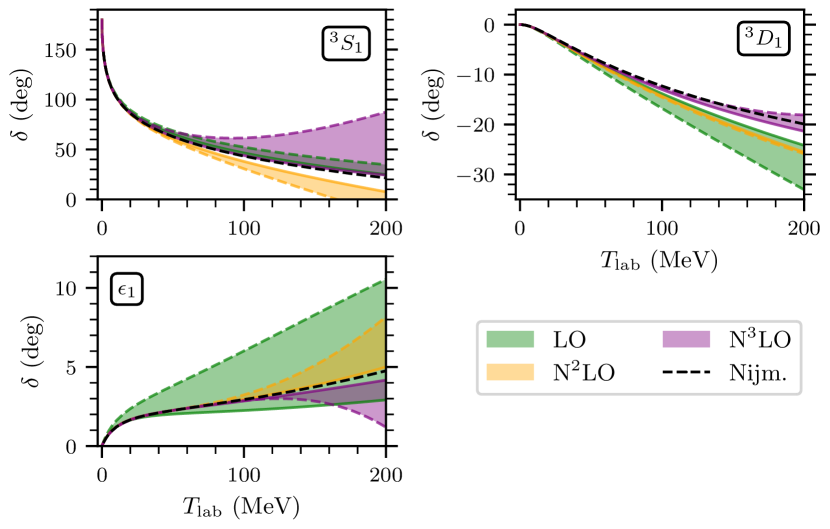
Figure 3: Predicted phase shifts in the ${}^{3}S_{1}\mathrm{-}^{3}D_{1}$ channel in the BB convention Blatt:1952zz as a function of scattering energy for the LEC calibration with corresponding ERE parameters in Table 3. The bands indicate the envelope of the cutoff variation; $\Lambda=500$ MeV (dashed line) and $\Lambda=2500$ MeV (solid line). The black dashed line shows phase shifts from the Nijmegen analysis Stoks:1993tb in the BB convention.

Table 3: LETs in the ${}^{3}S_{1}$ partial wave for different momentum cutoffs $\Lambda$. The parameters marked with a star ($*$) are used in the inference and are not predictions. The quoted errors only stem from the numerical extraction of the ERE parameters from the effective range function. Empirical ERE parameters are also shown.

${}^{3}S_{1}$ partial wave	$a$ [fm]	$r$ [fm]	$v_{2}$ [fm3]	$v_{3}$ [fm5]	$v_{4}$ [fm7]
Empirical (Ref. NavarroPerez:2014ovp )	5.42	1.75	0.045	0.67	$-3.94$
$\Lambda=500$ MeV
LO	$*$	$1.58(0)$	$-0.10(0)$	$0.89(0)$	$-5.5(2)$
N2LO	$*$	$*$	$0.14(0)$	$0.80(0)$	$-4.2(2)$
N3LO	$*$	$*$	$-0.06(0)$	$0.46(0)$	$-3.7(2)$
$\Lambda=750$ MeV
LO	$*$	$1.69(0)$	$0.01(0)$	$0.77(0)$	$-4.5(4)$
N2LO	$*$	$*$	$0.10(0)$	$0.77(0)$	$-4.2(4)$
N3LO	$*$	$*$	$0.01(0)$	$0.62(0)$	$-4.0(4)$
$\Lambda=1000$ MeV
LO	$*$	$1.69(0)$	$0.01(0)$	$0.77(0)$	$-4.6(4)$
N2LO	$*$	$*$	$0.09(0)$	$0.75(0)$	$-4.2(7)$
N3LO	$*$	$*$	$0.04(0)$	$0.67(0)$	$-4.0(4)$
$\Lambda=2500$ MeV
LO	$*$	$1.66(0)$	$-0.01(0)$	$0.79(0)$	$-4.7(2)$
N2LO	$*$	$*$	$0.09(0)$	$0.74(0)$	$-4.2(7)$
N3LO	$*$	$*$	$0.04(0)$	$0.67(2)$	$-4.0(9)$

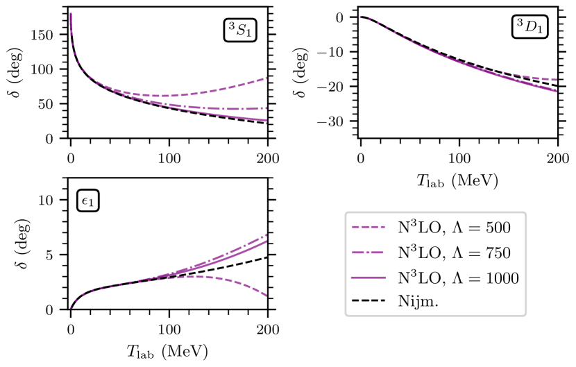
Figure 4: Predicted phase shifts in the ${}^{3}S_{1}\mathrm{-}^{3}D_{1}$ channel in the BB convention Blatt:1952zz as a function of scattering energy at N³LO for the LEC calibration with corresponding ERE parameters in Table 3. The purple dashed, dot-dashed, and solid lines correspond to momentum cutoffs $\Lambda=500$ MeV, $\Lambda=750$ MeV, and $\Lambda=1000$ MeV respectively. The black dashed line shows phase shifts from the Nijmegen analysis Stoks:1993tb in the BB convention.

The LECs in the ${}^{3}S_{1}\mathrm{-}^{3}D_{1}$ channel are fixed using calibration data that ensures a good description of both phase shifts and ERE parameters—the same principle as used in the ${}^{1}S_{0}$ partial wave. The empirical values for the ERE parameters NavarroPerez:2014ovp used in the inference are displayed in Table 3. At LO the only LEC, $C^{(0)}_{{}^{3}S_{1}}$, is inferred by reproducing the ${}^{3}S_{1}$ scattering length. The NLO contribution is zero and contains no LECs, but at N²LO there are three LECs: $C^{(1)}_{{}^{3}S_{1}}$, $D^{(0)}_{{}^{3}S_{1}}$ and $D^{(0)}_{SD}$. These are inferred by reproducing the scattering length ($a$), effective range ($r$), and the mixing angle $(\epsilon_{1})$ from the Nijmegen analysis at $T_{\mathrm{lab}}=50$ MeV Stoks:1993tb . The three LECs at N³LO: $C^{(2)}_{{}^{3}S_{1}}$, $D^{(1)}_{{}^{3}S_{1}}$ and $D^{(1)}_{SD}$ are perturbative corrections to the LECs at N²LO and are fixed using the same data as at N²LO. The LECs are inferred using momentum cutoffs $\Lambda=500,750,1000$ and 2500 MeV, where the intermediate cutoffs are used to get a better understanding of the residual cutoff dependence.

The resulting phase shifts for the extreme values of the cutoffs $\Lambda=500$ MeV and $\Lambda=2500$ MeV are shown in Fig. 3. The residual cutoff dependence should decrease as the chiral order increases. This is not observed at N³LO, since the phase shifts for $\Lambda=500$ MeV deviate significantly from both the Nijmegen and $\Lambda=2500$ MeV phase shifts. However, the results for $\Lambda=2500$ MeV show an excellent agreement with both empirical phase shifts, empirical ERE parameters, and similar studies Epelbaum:2003xx ; Epelbaum:2012ua .

LETs are computed from the effective range function using the same method as in the ${}^{1}S_{0}$ partial wave and the results are shown in Table 3. The LETs show an expected convergence order-by-order, where $v_{2}$ is the exception, and especially for $\Lambda=500$ MeV. This can likely be attributed to the small numerical value of $v_{2}$, which makes it harder to extract reliably—a fact that is also reflected in a larger relative error between extractions from different high-precision potentials compared to $v_{3}$ and $v_{4}$ NavarroPerez:2014ovp .

Both the LETs and phase shifts show a large residual cutoff dependence at N³LO reflecting the fact that the $\Lambda=500$ MeV result is deviating significantly from the results with higher cutoffs. The cutoff dependence is further illustrated in Fig. 4 which shows predicted phase shifts at N³LO for the lowest cutoffs $\Lambda=500,750,$ and 1000 MeV. It is observed that the deviation of the predicted phase shifts compared to the Nijmegen analysis increases as the cutoff decreases, which is consistent with the observed cutoff variation of LETs in Table 3. The residual cutoff dependence at N³LO seems to be under control if the cutoff is chosen sufficiently large, $\Lambda\gtrsim 750$ MeV. This large cutoff dependence for low cutoffs can have several explanations. It can be an indication that the convergence radius for the perturbative computations in the ${}^{3}S_{1}\mathrm{-}^{3}D_{1}$ channel is lower than expected, and the residual cutoff dependence signals that the perturbative series starts to diverge. It can also be an effect of a sub-optimal calibration procedure employed to fix the LECs. Another culprit can be the $c_{i}$ LECs parameterizing the strength of the sub-leading two-pion exchange. In Ref. Long:2012ve it was observed that some phase shifts at N³LO can be very sensitive to the employed values of the $c_{i}$ LECs, in line with the findings of Birse:2010jr . The explanation can also be that the lower cutoffs neglect relevant loop contributions from the iterated one-pion exchange at LO, reflected in the large error observed in the $\epsilon_{1}$ phase shift for $\Lambda=500$ MeV in Fig. 3—an effect that can be challenging to correct perturbatively. Detailed studies of the convergence of the perturbative expansion and possible connections to the $c_{i}$ LECs are left for future studies. It could also be interesting to address how the convergence is affected by using different regularization schemes, e.g., spectral function regularization Epelbaum:2003xx ; Epelbaum:2003gr , and by including the $\Delta(1232)$ isobar as an explicit degree of freedom.

4 Conclusions

In this study, we have computed LETs for $np$ scattering in $\chi$EFT to investigate the low-energy (long-range) behavior of the Long and Yang PC. The following conclusions can be made.

1. LETs can accurately be computed in perturbation theory both by directly using the scattering amplitudes (Eqs. 17, 18, 19 and 20) and by using phase shifts (Eq. 21). The observed simultaneous accuracy of LETs and low-energy phase shifts indicates that the low-energy description of the nuclear force seems to be captured in the employed perturbative PC for the considered $S$-waves.

2. The obtained LETs in the ${}^{1}S_{0}$ partial wave up to NLO are consistent with similar studies Epelbaum:2012ua ; Epelbaum:2015sha and the residual cutoff dependence in both LETs and phase shifts is small and consistent with expectations at each order. It is also shown that it is possible to get an excellent description of the ${}^{1}S_{0}$ phase shift at N³LO up to $T_{\mathrm{lab}}=100$ MeV.

3. Going beyond NLO in the ${}^{1}S_{0}$ partial wave does not provide LETs with increasing accuracy. This is contrary to expectations, since two-pion exchange enters at N²LO and is expected to provide a significant contribution to improving the low-energy description Baru:2015ira . Possible explanations for the lacking convergence can be that the two-pion exchange is not correctly captured in this PC, and/or that the employed procedure to calibrate the LECs is not adequate for perturbative calculations. Indeed, sources of uncertainty were neglected when inferring the LECs, and the analysis illustrated in Fig. 2 demonstrated that there is a large possibility of overfitting to the effective range parameters.

4. In the ${}^{3}S_{1}$ partial wave, the LETs reproduce the empirical ERE parameters while an accurate description of phase shifts up to at least $T_{\mathrm{lab}}=100$ MeV is kept—as long as the cutoff is taken large enough ($\Lambda\gtrsim 750$ MeV). This strongly suggests that sub-leading interaction potentials, and in particular the two-pion exchanges, are amendable to a perturbative treatment in this channel. For smaller cutoffs, a large residual cutoff dependence in both phase shifts and LETs is observed at N³LO. Further studies are needed to assess the origin of this larger-than-expected residual dependence.

In future studies, it would be valuable to quantify the extent to which overlooked sources of uncertainty in both data and models, along with choices made during the inference of LECs, influence the results. This can be effectively achieved within a Bayesian framework Furnstahl:2014xsa , wherein LECs are treated as stochastic variables. However, conducting a Bayesian inference of LECs may encounter challenges, including the risk of overfitting, and the emergence of spurious correlations among LECs at different orders. The latter is particularly prominent in a perturbative PC where the perturbative corrections to LECs naturally exhibit strong correlations. The results of this study confirm the effectiveness of LETs also in this perturbative PC which can be used as a tool to counteract overfitting LECs to high-energy data and ensuring that the fidelity of the low-energy description is maintained.

Acknowledgments O.T is grateful to Andreas Ekström, Christian Forssén and Daniel Phillips for helpful discussions as well as for providing feedback on the manuscript. This work was supported by the European Research Council (ERC) under the European Unions Horizon 2020 research and innovation program (Grant Agreement No. 758027) and the Swedish Research Council (Grant No. 2020-05127).

Appendix A Additional tables

This appendix contains some additional tables that summarize some LET results from the literature for the ${}^{1}S_{0}$ partial wave (Table 4) and the ${}^{3}S_{1}$ partial wave (Table 5).

Table 4: Collection of LET results in the ${}^{1}S_{0}$ partial wave from several studies. The parameters marked with a star ($*$) were used in the inference in the respective studies.

${}^{1}S_{0}$ partial wave	$a$ [fm]	$r$ [fm]	$v_{2}$ [fm3]	$v_{3}$ [fm5]	$v_{4}$ [fm7]
Mean Ref. NavarroPerez:2014ovp	$-23.735(16)$	2.68(3)	$-0.48(2)$	3.9(1)	$-19.6(5)$
N2LO WPC (DR) Ref. Epelbaum:2003xx	$-23.936$	2.73	$-0.46$	3.8	$-19.1$
NLO KSW from Ref. Cohen:1998jr	$*$	$*$	$-3.3$	18	$-108$
LO from Ref. Epelbaum:2012ua	$*$	1.5	$-1.9$	9.6(8)	$-37(10)$
NLO (pert.) from Ref. Epelbaum:2015sha	$*$	$*$	$-0.54(3)$	4.6(1)	$-29.3(5)$

Table 5: Collection of LET results in the ${}^{3}S_{1}$ partial wave. The parameters marked with a star ($*$) were used in the inference in the respective studies.

${}^{3}S_{1}$ partial wave	$a$ [fm]	$r$ [fm]	$v_{2}$ [fm3]	$v_{3}$ [fm5]	$v_{4}$ [fm7]
NijmII (Ref. PavonValderrama:2005ku )	5.419	1.753	0.0453	0.658	-4.191
Reid93 (Ref. PavonValderrama:2005ku )	5.423	1.756	0.0327	0.658	-4.193
NijmII (Ref. NavarroPerez:2014ovp )	5.4197(3)	1.75343(3)	0.04545(1)	0.6735(1)	-3.9414(8)
LO WPC (Ref. Epelbaum:2012ua )	$*$	1.60	$-0.05$	0.8(1)	$-4(1)$
N2LO WPC
(DR) (Ref. Epelbaum:2003xx )	5.416	1.756	0.04	0.67	$-4.1$
NLO KSW (Ref. Cohen:1998jr )	$*$	$*$	-0.95	4.6	-25.0

Appendix B Computing phase shifts perturbatively

The ${}^{1}S_{0}$ phase shift, $\delta(k)$, and on-shell scattering amplitude, $T(k,k)$, are related through Eq. 11 which simplifies to

$$e^{2i\delta}=1-i\pi km_{N}T(k,k),$$ (22)

where the quantum numbers are suppressed from the notation. By expressing both the phase shift and the amplitude in contributions at each chiral order according to Eqs. 10 and 12 and expanding both sides of Eq. 22 the following relations are obtained

$$\exp\left(2i\delta^{(0)}\right) =1-i\pi km_{N}T^{(0)}(k,k)$$ (23)

$$2i\delta^{(1)} =-i\pi km_{N}T^{(1)}(k,k)\exp\left(-2i\delta^{(0)}\right)$$ (24)

$$2i\delta^{(2)}-2\left(\delta^{(1)}\right)^{2} =-i\pi km_{N}T^{(2)}(k,k)\exp\left(-2i\delta^{(0)}\right)$$ (25)

$$2i\delta^{(3)}-4\delta^{(1)}\delta^{(2)}-\frac{4i}{3}\left(\delta^{(1)}\right)^{3} =-i\pi km_{N}T^{(3)}(k,k)\exp\left(-2i\delta^{(0)}\right).$$ (26)

From these equations, the phase shift corrections, $\delta^{(\nu)}$, can be obtained.

The computation in the coupled ${}^{3}S_{1}\mathrm{-}^{3}D_{1}$ channel is slightly more involved. The BB parametrization Blatt:1952zz of the unitary $2\times 2$ $S$-matrix reads

$$S=\begin{pmatrix}\cos{\epsilon}&\ -\sin{\epsilon}\\ \sin{\epsilon}&\ \cos{\epsilon}\end{pmatrix}\begin{pmatrix}e^{2i\delta_{-}}&\ 0\\ 0&\ e^{2i\delta_{+}}\end{pmatrix}\begin{pmatrix}\cos{\epsilon}&\ \sin{\epsilon}\\ -\sin{\epsilon}&\ \cos{\epsilon}\end{pmatrix}$$ (27)

where $\delta_{-}$ and $\delta_{+}$ are the eigen phase shifts corresponding to the ${}^{3}S_{1}$ and ${}^{3}D_{1}$ partial waves, respectively and $\epsilon$ is the mixing angle. Using Eq. 11 the phase shifts can be expressed as

$$\epsilon =\frac{1}{2}\arctan\left(\frac{2T^{sj}_{-+}}{T^{sj}_{--}-T^{sj}_{++}}\right)$$ (28)

$$\delta_{-}\left(k\right) =-\frac{i}{2}\log\left[1-\pi im_{N}k\left(\frac{T^{sj}_{--}+T^{js}_{++}}{2}+\frac{T^{sj}_{-+}}{\sin{2\epsilon}}\right)\right]$$ (29)

$$\delta_{+}\left(k\right) =-\frac{i}{2}\log\left[1-\pi im_{N}k\left(\frac{T^{sj}_{--}+T^{sj}_{++}}{2}-\frac{T^{sj}_{-+}}{\sin{2\epsilon}}\right)\right],$$ (30)

where the $\pm$ notation represent $\ell^{\prime},\ \ell=j\pm 1$. From the computed on-shell amplitudes $T^{(\nu)sj}_{\ell^{\prime}\ell}$ for orders $\nu=0,1,2,3$ the corresponding phase shifts $\big{(}\delta^{(\nu)}_{-},\delta^{(\nu)}_{+},\epsilon^{(\nu)}\big{)}$, $\nu=0,1,2,3$ are obtained by Taylor expanding Eqs. 28, 29 and 30 and matching chiral orders. This is completely analogous to the treatment of the ${}^{1}S_{0}$ partial wave and the treatment of the Stapp parametrization Stapp:1956mz in Refs. PhysRevC.85.034002 ; Thim:2024yks .

References

- \bibcommenthead
- (1) H.A. Bethe, Theory of the Effective Range in Nuclear Scattering. Phys. Rev. 76, 38–50 (1949). 10.1103/PhysRev.76.38
- (2) T.D. Cohen, J.M. Hansen, Low-energy theorems for nucleon-nucleon scattering. Phys. Rev. C 59, 13–20 (1999). 10.1103/PhysRevC.59.13. arXiv:nucl-th/9808038
- (3) S. Weinberg, Nuclear forces from chiral Lagrangians. Phys. Lett. B 251, 288–292 (1990). 10.1016/0370-2693(90)90938-3
- (4) S. Weinberg, Effective chiral Lagrangians for nucleon - pion interactions and nuclear forces. Nucl. Phys. B 363, 3–18 (1991). 10.1016/0550-3213(91)90231-L
- (5) E. Epelbaum, H.W. Hammer, U.G. Meissner, Modern Theory of Nuclear Forces. Rev. Mod. Phys. 81, 1773–1825 (2009). 10.1103/RevModPhys.81.1773. arXiv:0811.1338 [nucl-th]
- (6) R. Machleidt, D.R. Entem, Chiral effective field theory and nuclear forces. Phys. Rept. 503, 1–75 (2011). 10.1016/j.physrep.2011.02.001. arXiv:1105.2919 [nucl-th]
- (7) H.W. Hammer, S. König, U. van Kolck, Nuclear effective field theory: status and perspectives. Rev. Mod. Phys. 92(2), 025,004 (2020). 10.1103/RevModPhys.92.025004. arXiv:1906.12122 [nucl-th]
- (8) C. Ordonez, L. Ray, U. van Kolck, The Two nucleon potential from chiral Lagrangians. Phys. Rev. C 53, 2086–2105 (1996). 10.1103/PhysRevC.53.2086. arXiv:hep-ph/9511380
- (9) U. van Kolck, Few nucleon forces from chiral Lagrangians. Phys. Rev. C 49, 2932–2941 (1994). 10.1103/PhysRevC.49.2932
- (10) C. Ordonez, L. Ray, U. van Kolck, Nucleon-nucleon potential from an effective chiral Lagrangian. Phys. Rev. Lett. 72, 1982–1985 (1994). 10.1103/PhysRevLett.72.1982
- (11) D.R. Entem, N. Kaiser, R. Machleidt, Y. Nosyk, Dominant contributions to the nucleon-nucleon interaction at sixth order of chiral perturbation theory. Phys. Rev. C 92(6), 064,001 (2015). 10.1103/PhysRevC.92.064001. arXiv:1505.03562 [nucl-th]
- (12) P. Reinert, H. Krebs, E. Epelbaum, Semilocal momentum-space regularized chiral two-nucleon potentials up to fifth order. Eur. Phys. J. A 54(5), 86 (2018). 10.1140/epja/i2018-12516-4. arXiv:1711.08821 [nucl-th]
- (13) E. Epelbaum, A. Nogga, W. Gloeckle, H. Kamada, U.G. Meissner, H. Witala, Three nucleon forces from chiral effective field theory. Phys. Rev. C 66, 064,001 (2002). 10.1103/PhysRevC.66.064001. arXiv:nucl-th/0208023
- (14) G. Hagen, et al., Neutron and weak-charge distributions of the 48Ca nucleus. Nature Phys. 12(2), 186–190 (2015). 10.1038/nphys3529. arXiv:1509.07169 [nucl-th]
- (15) P. Arthuis, C. Barbieri, M. Vorabbi, P. Finelli, Computation of Charge Densities for Sn and Xe Isotopes. Phys. Rev. Lett. 125(18), 182,501 (2020). 10.1103/PhysRevLett.125.182501. arXiv:2002.02214 [nucl-th]
- (16) B. Hu, et al., Ab initio predictions link the neutron skin of 208Pb to nuclear forces. Nature Phys. 18(10), 1196–1200 (2022). 10.1038/s41567-022-01715-8. arXiv:2112.01125 [nucl-th]
- (17) A. Nogga, R.G.E. Timmermans, U. van Kolck, Renormalization of one-pion exchange and power counting. Phys. Rev. C 72, 054,006 (2005). 10.1103/PhysRevC.72.054006. arXiv:nucl-th/0506005
- (18) U. van Kolck, The Problem of Renormalization of Chiral Nuclear Forces. Front. in Phys. 8, 79 (2020). 10.3389/fphy.2020.00079. arXiv:2003.06721 [nucl-th]
- (19) B. Long, U. van Kolck, Renormalization of Singular Potentials and Power Counting. Annals Phys. 323, 1304–1323 (2008). 10.1016/j.aop.2008.01.003. arXiv:0707.4325 [quant-ph]
- (20) S.R. Beane, P.F. Bedaque, L. Childress, A. Kryjevski, J. McGuire, U. van Kolck, Singular potentials and limit cycles. Phys. Rev. A 64, 042,103 (2001). 10.1103/PhysRevA.64.042103. URL https://link.aps.org/doi/10.1103/PhysRevA.64.042103
- (21) E. Epelbaum, A.M. Gasparyan, J. Gegelia, U.G. Meißner, How (not) to renormalize integral equations with singular potentials in effective field theory. Eur. Phys. J. A 54(11), 186 (2018). 10.1140/epja/i2018-12632-1. arXiv:1810.02646 [nucl-th]
- (22) D.B. Kaplan, M.J. Savage, M.B. Wise, A New expansion for nucleon-nucleon interactions. Phys. Lett. B 424, 390–396 (1998). 10.1016/S0370-2693(98)00210-X. arXiv:nucl-th/9801034
- (23) D.B. Kaplan, M.J. Savage, M.B. Wise, Two nucleon systems from effective field theory. Nucl. Phys. B 534, 329–355 (1998). 10.1016/S0550-3213(98)00440-4. arXiv:nucl-th/9802075
- (24) S. Fleming, T. Mehen, I.W. Stewart, NNLO corrections to nucleon-nucleon scattering and perturbative pions. Nucl. Phys. A 677, 313–366 (2000). 10.1016/S0375-9474(00)00221-9. arXiv:nucl-th/9911001
- (25) T.D. Cohen, J.M. Hansen, Testing low-energy theorems in nucleon-nucleon scattering. Phys. Rev. C 59, 3047–3051 (1999). 10.1103/PhysRevC.59.3047. arXiv:nucl-th/9901065
- (26) V.G.J. Stoks, R.A.M. Klomp, M.C.M. Rentmeester, J.J. de Swart, Partial wave analaysis of all nucleon-nucleon scattering data below 350-MeV. Phys. Rev. C 48, 792–815 (1993). 10.1103/PhysRevC.48.792
- (27) R. Navarro Pérez, J.E. Amaro, E. Ruiz Arriola, The low-energy structure of the nucleon–nucleon interaction: statistical versus systematic uncertainties. J. Phys. G 43(11), 114,001 (2016). 10.1088/0954-3899/43/11/114001. arXiv:1410.8097 [nucl-th]
- (28) S.I. Ando, C.H. Hyun, Effective range corrections from effective field theory with di-baryon fields and perturbative pions. Phys. Rev. C 86, 024,002 (2012). 10.1103/PhysRevC.86.024002. arXiv:1112.2456 [nucl-th]
- (29) M. Pavon Valderrama, E. Ruiz Arriola, Renormalization of singlet N N scattering with one pion exchange and boundary conditions. Phys. Lett. B 580, 149–156 (2004). 10.1016/j.physletb.2003.11.037. arXiv:nucl-th/0306069
- (30) E. Epelbaum, W. Glockle, U.G. Meissner, The Two-nucleon system at next-to-next-to-next-to-leading order. Nucl. Phys. A 747, 362–424 (2005). 10.1016/j.nuclphysa.2004.09.107. arXiv:nucl-th/0405048
- (31) E. Epelbaum, W. Gloeckle, U.G. Meissner, Improving the convergence of the chiral expansion for nuclear forces. 2. Low phases and the deuteron. Eur. Phys. J. A 19, 401–412 (2004). 10.1140/epja/i2003-10129-8. arXiv:nucl-th/0308010
- (32) E. Epelbaum, J. Gegelia, Regularization, renormalization and ’peratization’ in effective field theory for two nucleons. Eur. Phys. J. A 41, 341–354 (2009). 10.1140/epja/i2009-10833-3. arXiv:0906.3822 [nucl-th]
- (33) V. Baru, E. Epelbaum, A.A. Filin, J. Gegelia, Low-energy theorems for nucleon-nucleon scattering at unphysical pion masses. Phys. Rev. C 92(1), 014,001 (2015). 10.1103/PhysRevC.92.014001. arXiv:1504.07852 [nucl-th]
- (34) V. Baru, E. Epelbaum, A.A. Filin, Low-energy theorems for nucleon-nucleon scattering at MeV. Phys. Rev. C 94(1), 014,001 (2016). 10.1103/PhysRevC.94.014001. arXiv:1604.02551 [nucl-th]
- (35) B. Long, C.J. Yang, Short-range nuclear forces in singlet channels. Phys. Rev. C 86, 024,001 (2012). 10.1103/PhysRevC.86.024001. arXiv:1202.4053 [nucl-th]
- (36) B. Long, C.J. Yang, Renormalizing chiral nuclear forces: A case study of . Phys. Rev. C 84, 057,001 (2011). 10.1103/PhysRevC.84.057001. URL https://link.aps.org/doi/10.1103/PhysRevC.84.057001
- (37) B. Long, C.J. Yang, Renormalizing chiral nuclear forces: Triplet channels. Phys. Rev. C 85, 034,002 (2012). 10.1103/PhysRevC.85.034002. URL https://link.aps.org/doi/10.1103/PhysRevC.85.034002
- (38) O. Thim, E. May, A. Ekström, C. Forssén, Bayesian analysis of chiral effective field theory at leading order in a modified Weinberg power counting approach. Phys. Rev. C 108(5), 054,002 (2023). 10.1103/PhysRevC.108.054002. arXiv:2302.12624 [nucl-th]
- (39) O. Thim, A. Ekström, C. Forssén, Perturbative computations of neutron-proton scattering observables using renormalization-group invariant EFT up to N3LO (2024). arXiv:2402.15325 [nucl-th]
- (40) C.J. Yang, A. Ekström, C. Forssén, G. Hagen, Power counting in chiral effective field theory and nuclear binding. Phys. Rev. C 103(5), 054,304 (2021). 10.1103/PhysRevC.103.054304. arXiv:2011.11584 [nucl-th]
- (41) A. Ekström, et al., Optimized Chiral Nucleon-Nucleon Interaction at Next-to-Next-to-Leading Order. Phys. Rev. Lett. 110(19), 192,502 (2013). 10.1103/PhysRevLett.110.192502. arXiv:1303.4674 [nucl-th]
- (42) M.R. Schindler, D.R. Phillips, Bayesian Methods for Parameter Estimation in Effective Field Theories. Annals Phys. 324, 682–708 (2009). 10.1016/j.aop.2008.09.003. [Erratum: Annals Phys. 324, 2051–2055 (2009)]. arXiv:0808.3643 [hep-ph]
- (43) R.J. Furnstahl, D.R. Phillips, S. Wesolowski, A recipe for EFT uncertainty quantification in nuclear physics. J. Phys. G 42(3), 034,028 (2015). 10.1088/0954-3899/42/3/034028. arXiv:1407.0657 [nucl-th]
- (44) H.W. Grießhammer, Assessing Theory Uncertainties in EFT Power Countings from Residual Cutoff Dependence. PoS CD15, 104 (2016). 10.22323/1.253.0104. arXiv:1511.00490 [nucl-th]
- (45) E. Epelbaum, J. Gegelia, Weinberg’s approach to nucleon–nucleon scattering revisited. Phys. Lett. B 716, 338–344 (2012). 10.1016/j.physletb.2012.08.025. arXiv:1207.2420 [nucl-th]
- (46) E. Epelbaum, A.M. Gasparyan, J. Gegelia, H. Krebs, 1S0 nucleon-nucleon scattering in the modified Weinberg approach. Eur. Phys. J. A 51(6), 71 (2015). 10.1140/epja/i2015-15071-6. arXiv:1501.01191 [nucl-th]
- (47) L. Contessi, A. Lovato, F. Pederiva, A. Roggero, J. Kirscher, U. van Kolck, Ground-state properties of 4He and 16O extrapolated from lattice QCD with pionless EFT. Phys. Lett. B 772, 839–848 (2017). 10.1016/j.physletb.2017.07.048. arXiv:1701.06516 [nucl-th]
- (48) D. Siemens, J. Ruiz de Elvira, E. Epelbaum, M. Hoferichter, H. Krebs, B. Kubis, U.G. Meißner, Reconciling threshold and subthreshold expansions for pion–nucleon scattering. Phys. Lett. B 770, 27–34 (2017). 10.1016/j.physletb.2017.04.039. arXiv:1610.08978 [nucl-th]
- (49) R. Peng, S. Lyu, B. Long, Perturbative chiral nucleon–nucleon potential for the partial wave. Commun. Theor. Phys. 72(9), 095,301 (2020). 10.1088/1572-9494/aba251. arXiv:2011.13186 [nucl-th]
- (50) M.I. Haftel, F. Tabakin, Nuclear saturation and the smoothness of nucleon-nucleon potentials. Nucl. Phys. A 158, 1–42 (1970). 10.1016/0375-9474(70)90047-3
- (51) W. Glöckle, The Quantum Mechanical Few-body Problem (Springer-Verlag, Berlin Heidelberg, 1983)
- (52) J.R. Taylor, Scattering Theory: The quantum Theory on Nonrelativistic Collisions (Wiley, New York, 1972)
- (53) M. Pavon Valderrama, E. Ruiz Arriola, Low-energy NN scattering at next-to-next-to-next-to-next-to-leading order for partial waves with j 5. Phys. Rev. C 72, 044,007 (2005). 10.1103/PhysRevC.72.044007
- (54) J.M. Blatt, L.C. Biedenharn, The Angular Distribution of Scattering and Reaction Cross Sections. Rev. Mod. Phys. 24, 258–272 (1952). 10.1103/RevModPhys.24.258
- (55) M.C. Birse, Deconstructing nucleon-nucleon scattering. Eur. Phys. J. A 46, 231–240 (2010). 10.1140/epja/i2010-11034-9. arXiv:1007.0540 [nucl-th]
- (56) E. Epelbaum, W. Gloeckle, U.G. Meissner, Improving the convergence of the chiral expansion for nuclear forces. 1. Peripheral phases. Eur. Phys. J. A 19, 125–137 (2004). 10.1140/epja/i2003-10096-0. arXiv:nucl-th/0304037
- (57) H.P. Stapp, T.J. Ypsilantis, N. Metropolis, Phase shift analysis of 310-MeV proton proton scattering experiments. Phys. Rev. 105, 302–310 (1957). 10.1103/PhysRev.105.302