Moduli spaces of quadratic differentials: Abel-Jacobi map and deformation

Abstract.

We study the moduli space of framed quadratic differentials with prescribed singularities parameterized by a decorated marked surface with punctures (DMSp), where simple zeros, double poles and higher order poles respectively correspond to decorations, punctures and boundary components. We show that the fundamental group of this space equals the kernel of the Abel-Jacobi map from the surface mapping class group of DMSp to the first homology group of the marked surface (without decorations/punctures). Moreover, a universal cover of this space is given by the space of stability conditions on the associated 3-Calabi-Yau category.

Furthermore, when we partial compactify and orbifold this moduli space by allowing the collision of simple zeros and some of the double poles, the resulting moduli space is isomorphic to a quotient of the space of stability conditions on the deformed (with respect to those collidable double poles) 3-Calabi-Yau category.

Key words: quadratic differentials, twist groups, flip graphs, Abel-Jacobi maps, stability conditions

1. Introduction

1.1. Topology of moduli spaces of quadratic differentials

The moduli spaces of abelian/quadratic differentials are classical objects of study in dynamical systems, which also naturally interact with topology, algebraic geometry and, recently, representation theory of algebras. For instance, the topology of moduli spaces has attracted a lot of attention.

Connected components

Kontsevich-Zorich [KZ2] classified the connected components of the space of holomorphic abelian differentials; later Lanneau [Lan] and Boissy [Boi] treated the case of meromorphic quadratic differentials; more recently, Chen-Gendron [CG] extended this the case of $k$-differentials. In most of these cases, the components are classified by spin invariants, hyper-ellipticity and torsion conditions.

Fundamental groups

The next interesting and challenging question is the calculation of (orbifold) fundamental groups of components of these spaces. Until now, few cases have been known: see [Wal, Ham, CS2] for the studies on certain quotient groups of the fundamental groups of such types, [FM] and [LM] for the genus 2 and 3 cases respectively.

In the previous work with King [KQ2], we calculated the connected components and fundamental groups of moduli spaces of quadratic differentials with only simple zeros and higher order poles, in which case, the prescribed singularities are encoded by a decorated marked surface (DMS) $\mathbf{S}_{\Delta}$. One of the key ingredients is the introduction of the braid twist group $\operatorname{BT}(\mathbf{S}_{\Delta})\lhd\operatorname{MCG}(\mathbf{S}_{\Delta})$ of $\mathbf{S}_{\Delta}$ in [Qy2], generated by the braid twists along any closed arcs). Such a group is a (usually proper) normal subgroup of the surface braid group $\operatorname{SBr}(\mathbf{S}_{\Delta})$. The motivation came from the study of the spherical twist group of the Calabi-Yau-3 category associated to $\mathbf{S}_{\Delta}$, where these two (braid and spherical) twist groups can be naturally identified ([Qy2, Thm. 1]).

In this work, we investigate the case with simple zeros, higher order poles and also double poles. The first key observation is that the braid twist group is in fact, the kernel of the Abel-Jacobi map. In the finite area case (no double or higher order poles), this map was considered in [Wal].

Topological Abel-Jacobi maps

We fix a Riemann surface $\mathbf{X}$ and consider the quadratic differential $\phi$ of prescribed singularity type

$$(\mathbf{w}_{\operatorname{fin}}=\mathbf{w}_{\geq-1},\mathbf{w}_{\operatorname{inf}}=\mathbf{w}_{\leq-2}),$$

where $\mathbf{w}_{\operatorname{fin}}$ and $\mathbf{w}_{\operatorname{inf}}$ are the collections of the finite/infinite singularities, respectively, represented by their orders. The numerical datum is encoded by a weighted DMS with punctures, $\mathbf{S}_{\Delta}^{\text{\Sun}}$ which is the real blow-up of $\mathbf{X}$ with respect to $\phi$ (as a topological surface). The weighted decorations in $\Delta$ are finite singularities (=zeros and simple poles) in $\mathbf{w}_{\operatorname{fin}}$; the punctures in ☉ are order two poles in $\mathbf{w}_{-2}$; the marked points $\mathbf{M}\subset\partial\mathbf{S}$ on the boundary components correspond to (the distinguish directions at) higher order poles in $\mathbf{w}_{\leq-3}$. We will mainly focus on the moduli space $\operatorname{FQuad}(\mathbf{S}^{\text{\Sun}})$ of $\mathbf{S}^{\text{\Sun}}$-framed quadratic differentials. It is a manifold and a $\operatorname{MCG}(\mathbf{S}^{\text{\Sun}})$-covering of the (unframed) moduli space $\operatorname{Quad}(\mathbf{S}^{\text{\Sun}})$.

Each element in $\operatorname{FQuad}(\mathbf{S}^{\text{\Sun}})$ naturally maps to a configuration $\Delta$ of weighted points on $\mathbf{X}$ with special marking $\mathbf{w}_{\operatorname{inf}}$. The classical Abel-Jacobi map $\operatorname{AJ}^{\mathbf{w}_{\leq-3}}$ maps special marking $\mathbf{w}_{\leq-3}(\subset\mathbf{w}_{\operatorname{inf}})$, regarded as a divisor of $\mathbf{X}$, to a line bundle in the Picard variety $\operatorname{Pic}(\mathbf{X},\mathbf{w}_{\leq-3})$. Note that we forget about the punctures in $\text{\Sun}=\mathbf{w}_{-2}$ here. Then we obtain the following morphisms:

$$\operatorname{FQuad}(\mathbf{S}^{\text{\Sun}})\to\operatorname{conf}_{\Delta}(\mathbf{X},\mathbf{w}_{\operatorname{inf}})\xrightarrow{\operatorname{AJ}^{\mathbf{w}_{\leq-3}}}\operatorname{Pic}(\mathbf{X},\mathbf{w}_{\leq-3}).$$ (1.1)

Taking $\pi_{1}$ of these spaces, we obtain a sequence of maps:

$$\pi_{1}\operatorname{FQuad}(\mathbf{S}^{\text{\Sun}})\xrightarrow{\Xi}\operatorname{SBr}(\mathbf{S}^{\text{\Sun}}_{\Delta})\xrightarrow{\operatorname{AJ}}\operatorname{\bf H}_{1}(\mathbf{S}),$$ (1.2)

where the second term is the surface braid group and the last term is the first homology. We call the map $\operatorname{AJ}$ induced from $\operatorname{AJ}^{\mathbf{w}_{\operatorname{inf}}}$ the (topological) Abel-Jacobi map.

We will focus on the simple zero case, i.e. $\mathbf{w}_{\operatorname{fin}}=\mathbf{w}_{1}$. We will also consider the Teichmüller framed (i.e. $\mathbf{S}_{\Delta}^{\text{\Sun}}$-framed) version $\operatorname{FQuad}(\mathbf{S}_{\Delta}^{\text{\Sun}})$, which is the $\operatorname{MCG}(\mathbf{S}_{\Delta}^{\text{\Sun}})$-covering of $\operatorname{Quad}(\mathbf{S}^{\text{\Sun}})$. The following is the main result of the paper (Theorem 6.9).

Theorem 1.1.

Let $\mathbf{S}_{\Delta}^{\text{\Sun}}$ be a DMS with punctures. There is a short exact sequence

$$1\to\pi_{1}\operatorname{FQuad}(\mathbf{S}^{\text{\Sun}})\xrightarrow{\Xi}\operatorname{SBr}(\mathbf{S}_{\Delta}^{\text{\Sun}})\xrightarrow{\operatorname{AJ}}\operatorname{\bf H}_{1}(\mathbf{S})\to 1$$ (1.3)

Moreover, we have

$$\begin{cases}\pi_{1}\operatorname{FQuad}^{\mathbb{T}}(\mathbf{S}_{\Delta}^{\text{\Sun}})=1,\\ \pi_{0}\operatorname{FQuad}(\mathbf{S}_{\Delta}^{\text{\Sun}})\cong\operatorname{\bf H}_{1}(\mathbf{S}),\end{cases}$$ (1.4)

where $\operatorname{FQuad}^{\mathbb{T}}(\mathbf{S}_{\Delta}^{\text{\Sun}})$ is any connected component of $\operatorname{FQuad}(\mathbf{S}_{\Delta}^{\text{\Sun}})$.

The short exact sequence (1.3) is equivalent to (Corollary 6.11):

$$1\to\pi_{1}\operatorname{Quad}(\mathbf{S}^{\text{\Sun}})\xrightarrow{\Xi}\operatorname{MCG}(\mathbf{S}_{\Delta}^{\text{\Sun}})\xrightarrow{\widehat{\operatorname{AJ}}}\operatorname{\bf H}_{1}(\mathbf{S})\to 1,$$ (1.5)

where $\operatorname{Quad}(\mathbf{S}^{\text{\Sun}})$ is the unframed orbifold, which will appear in the later discussion.

When $\text{\Sun}=\varnothing$, the theorem is a slight improvement of the main result in [KQ2].

In the works [Wal, Ham, CS2], the authors studied maps similar to (1.2) and described the image of the corresponding $\Xi$. In our case, the most challenging part is the injectivity of $\Xi$. Notice that in general, injectivity does not holds, cf. [Ham, Rem. 12.4] and [Gia, Thm. A].

$K(\pi,1)$-conjecture and categorification

In [KZ1], Kontsevich-Zorich conjectured that ‘each connected component of (a stratum of the) moduli space of quadratic differentials has homotopy type $K(\pi,1)$ for $\pi$ which is a group commensurable with some mapping class group’. At least in our case (i.e. all finite singularities are simple zeros), we believe that is true. In fact, it is closely related to the contractibility conjecture for the spaces of stability conditions.

The notion of stability condition on triangulated categories was introduced by Bridgeland [Bri], with motivations coming from $\Pi$-stability in string theory. By the work of [HKK, CHQ], any connected component of a moduli space of quadratic differentials with prescribed singularity type $\mathbf{S}^{\text{\Sun}}_{\mathbf{w}_{\operatorname{fin}}}$ can be realized by the space of stability conditions on some triangulated category $\operatorname{\mathcal{D}}$:

$$\operatorname{FQuad}^{\mathbb{T}}(\mathbf{S}^{\text{\Sun}}_{\mathbf{w}_{\operatorname{fin}}})\cong\operatorname{Stab}^{\circ}(\operatorname{\mathcal{D}})$$

Such a category $\operatorname{\mathcal{D}}$ is not unique and can be chosen to be Calabi-Yau. One can consider that $\operatorname{Stab}\operatorname{\mathcal{D}}$ provides a categorification of the moduli space; other topological operations (e.g. collision and collapsing subsurface) may also be understood by some categorical operations (e.g. taking Verdier quotient). In particular, we will use the 3-Calabi-Yau categories $\operatorname{\mathcal{D}}_{3}(\mathbf{S}_{\Delta}^{\text{\Sun}})$ constructed in [CHQ], to prove the main result above. More precisely, we show the following (Theorem 6.8).

Theorem 1.2.

$\operatorname{Stab}^{\circ}(\operatorname{\mathcal{D}}_{3}(\mathbf{S}_{\Delta}^{\text{\Sun}}))$ is simply connected and hence is a universal cover of $\operatorname{FQuad}(\mathbf{S}^{\text{\Sun}})$.

Donaldson-Thomas (DT) invariants and quantum dilogarithm identities

Motivated by classical curve-counting problems, Thomas [Tho] proposed the so-called DT-invariants to count stable sheaves on Calabi–Yau 3-folds. Kontsevich–Soibelman [KS1, KS2] generalized their work and formalized a way of counting semistable objects in 3-Calabi–Yau triangulated ($A_{\infty}$-)categories (or counting BPS states in physics terminology), using the so-called motivic DT-invariants. The quantum version of DT-invariants can be calculated via a product of quantum dilogarithms cf. [Ke2, Rei, KS1, KS2, KW]. Recently Haiden [Hai] and Kidwai-Williams [KW] gave formulae for calculating the quantum DT-invariants in the surface case by counting saddle trajectories and ring domains

The point is that one can think of the DT-invariants of abelian categories (or hearts of some triangulated category) as a function on the spaces of stability conditions. It is constant in a fixed cell and changes values when crossing a wall (of the first kind). The fact that the product is an invariant is due to quantum dilogarithm identities (QDI). In many cases, the QDI reduce to the pentagon identity (and the trivial commutation relation or square identity), (e.g. [Qy1] for the Dynkin case, cf. [Na1, Na2]). In the marked surface case, such a reducibility (to square/pentagon identity) is equivalent to the fact that the fundamental group of the unoriented flip exchange graph $\underline{\operatorname{EG}}(\mathbf{S}^{\text{\Sun}})$ of triangulations is generated by squares and pentagons, cf. Theorem 3.1 for the classical result, [FST, Thm. 10.2] for the cluster case and our slight generalization Proposition B.2. Such results interpreted as local simply connectedness.

1.2. Techniques

Mixed twist group

The surface braid group $\operatorname{SBr}(\mathbf{S}_{\Delta}^{\text{\Sun}})$ was first introduced by Zariski (naturally generalizing Artin’s geometric definition) and was rediscovered by Fox (cf. the survey [GJP, § 2] and the references). There are two types of standard generators: the braid twist and the L-twists (point-pushing diffeomorphisms) see Figure 2 or Figure 1 for the monodromy version in the moduli spaces.

   

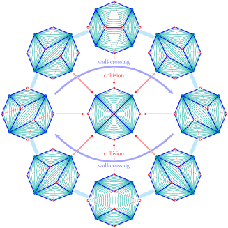
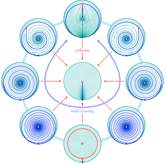
Figure 1. Monodromies/loops in moduli spaces as L-twist/braid twist

The first step of proving Theorem 1.1 is to understand the kernel of the Abel-Jacobi map in (1.3). For this purpose, we introduce the mixed twist groups $\operatorname{MT}(\mathbf{S}_{\Delta}^{\text{\Sun}\mid\leftmoon})$, which is the subgroup of $\operatorname{SBr}(\mathbf{S}_{\Delta}^{\text{\Sun}})$ generated by all braid twists and the L-twists that wind a puncture in a chosen subset $\leftmoon$ of ☉. Then we prove the following (Theorem 2.6 and Theorem 2.12).

Theorem 1.3.

The mixed twist group $\operatorname{MT}(\mathbf{S}_{\Delta}^{\text{\Sun}\mid\leftmoon})$ is the kernel of the (relative) Abel-Jacobi map $\operatorname{AJ}^{\text{\Sun}}_{\leftmoon}$:

$$\operatorname{MT}(\mathbf{S}_{\Delta}^{\text{\Sun}\mid\leftmoon})=\ker\big{(}\operatorname{SBr}(\mathbf{S}_{\Delta}^{\text{\Sun}})\xrightarrow{\operatorname{AJ}^{\text{\Sun}}_{\leftmoon}}\operatorname{\bf H}_{1}(\mathbf{S}^{{\rightmoon}})\big{)},$$ (1.6)

which admits a finite presentation in Theorem 2.12.

In particular, the biggest one is

$$\operatorname{MT}(\mathbf{S}_{\Delta}^{\text{\Sun}})=\operatorname{MT}(\mathbf{S}_{\Delta}^{\text{\Sun}\mid\text{\Sun}})=\ker\operatorname{AJ}\cong\pi_{1}\operatorname{FQuad}(\mathbf{S}^{\text{\Sun}})$$ (1.7)

for $\operatorname{AJ}=\operatorname{AJ}^{\text{\Sun}}_{\text{\Sun}}$ that appears in (1.4), and the smallest mixed twist group is the braid twist group $\operatorname{BT}(\mathbf{S}_{\Delta}^{\text{\Sun}})=\operatorname{MT}(\mathbf{S}_{\Delta}^{\text{\Sun}\mid\varnothing})=\ker\operatorname{AJ}^{\text{\Sun}}_{\varnothing}$.

Flip groupoid and flip twist groups

The other ingredient of proving Theorem 1.1 is the study of fundamental groups of oriented flip graphs. As mentioned in the DT-invariant paragraph, QDI is equivalent to the fact that $\pi_{1}\underline{\operatorname{EG}}(\mathbf{S}^{\text{\Sun}})$ is generated by unoriented squares and pentagons. We need to analyze the fundamental group $\pi_{1}\operatorname{FG}(\mathbf{S}_{\Delta}^{\text{\Sun}})$ of the flip graph of decorated triangulations of $\mathbf{S}_{\Delta}^{\text{\Sun}}$. There are four types of basic loops:

• The squares and pentagons lifted from $\pi_{1}\underline{\operatorname{EG}}(\mathbf{S}^{\text{\Sun}})$, see the left two pictures in Figure 11.

• The fat dumbbell hexagons introduced in [KQ2], see the right pictures in Figure 11.

• The new thin dumbbell hexagons, see Figure 18 (and cf. Figure 13).

• The new symmetric hexagons, see Figure 19 (and cf. Figure 13).

When imposing these loops/relations in the oriented version $\operatorname{FG}(\mathbf{S}^{\text{\Sun}})$ of flip graph for $\mathbf{S}^{\text{\Sun}}$, e.g., the purple graph in the right picture of Figure 10, we obtain the flip groupoid $\operatorname{\mathcal{FG}}(\mathbf{S}^{\text{\Sun}})$, as a generalization of cluster exchange groupoid introduced in [KQ2]. The subgroup of the point group at a triangulation $\mathrm{T}$ of $\pi_{1}\operatorname{\mathcal{FG}}(\mathbf{S}^{\text{\Sun}})$, generated by local flip twists, is the flip twist group $\operatorname{FT}(\mathrm{T})$, cf. Definition 4.3. We show that there is a natural isomorphism between a flip twist group and the corresponding mixed twist group (Theorem 5.8):

$$\operatorname{FT}(\mathrm{T})\cong\operatorname{MT}(\mathbf{S}_{\Delta}^{\text{\Sun}\mid\leftmoon(\mathbb{T})}),$$ (1.8)

where $\mathrm{T}$ is the triangulation of $\mathbf{S}^{\text{\Sun}}$ induced from a triangulation $\mathbb{T}$ of $\mathbf{S}_{\Delta}^{\text{\Sun}}$, forgetting about the decorations, and $\leftmoon(\mathbb{T})$ is the set of $\mathbb{T}$-isolated punctures (which are in self-folded $\mathbb{T}$-triangles).

A highlight of the proof is that the higher braid relation $\eta\delta\eta\delta=\delta\eta\delta\eta$ decomposes into 2 thin dumbbell hexagons and 2 symmetric hexagons as shown in Figure 14, which is very different from the other decomposition (via folding in cluster theory, cf. [HHQ]) into non-symmetric hexagons shown in Figure 15.

1.3. Partial compactification with orbifolding via deformation

After we study the mixed/flip twist groups, there is a strong hint of studying the various compactifications of $\operatorname{Quad}(\mathbf{S}_{\Delta}^{\text{\Sun}})$, in particular their categorifications using spaces of stability conditions. Recently, there are many works on the topic of compactifying spaces of stability conditions, including: [BDL, KKO] of Thurston type compactification; [Bol, BPPW] of partial compactification and [BMQS, BMS] towards multi-scale compactification in the sense of [BCGGM]. In Appendix B, we give a result of a similar nature.

The other natural moduli space

The moduli space $\operatorname{FQuad}(\mathbf{S}^{\text{\Sun}})$ and 3-Calabi-Yau category $\operatorname{\mathcal{D}}_{3}(\mathbf{S}_{\Delta}^{\text{\Sun}})$ in Theorem 1.2 are the natural ones associated to $\mathbf{S}^{\text{\Sun}}$ from the point of view of dynamical systems and of higher categories (i.e. perverse schobers, cf. [CHQ]). Also, recent work [KW] suggests the same from the point of view of DT-theory (and mathematical physics),

However, they are unnatural from the point of view of cluster theory and representation theory of algebras (cf. [FST, BS]), at least for the first glance. Indeed, associated to a triangulation $\mathrm{T}$ of $\mathbf{S}^{\text{\Sun}}$, the quiver with potential $Q_{\mathrm{T}}^{\text{\Sun}}$ with 3-cycles potential $W_{\mathrm{T}}^{\text{\Sun}}$ for $\operatorname{\mathcal{D}}_{3}(\mathbf{S}_{\Delta}^{\text{\Sun}})$ is degenerate, in the sense of [DWZ]. On the other hand, the unique non-degenerate quiver with potential $(Q_{\mathrm{T}}^{\text{\YinYang}},W_{\mathrm{T}}^{\text{\YinYang}})$ is the cluster favorite (cf. [L-F]). Indeed, the mutations of which match the original quiver mutations in the sense of [FZ] and the Jacobian algebras are of skew-gentle type, generalizing (and including) the type $D_{n}$ and $\widetilde{D_{n}}$. Fomin-Shapiro-Thurston [FST] introduced the extra $\mathbb{Z}/_{2}$ symmetry according to cluster theory, for each puncture (which we will call it a vortex). The corresponding interpretation in the moduli spaces of quadratic differentials is the inclusion of signs of residue at double poles and allowing the collision of simple zeros and double poles, cf. [GMN, BS].

The comparison

In the main theorem

$$\operatorname{Quad}(\mathbf{S}^{\text{\YinYang}})=\operatorname{FQuad}(\mathbf{S}^{\text{\YinYang}})/\operatorname{MCG}(\mathbf{S}^{\text{\YinYang}})\cong\operatorname{Stab}^{\circ}(\operatorname{\mathcal{D}}_{3}(\mathbf{S}^{\text{\YinYang}}))/\operatorname{Aut}^{\circ}$$ (1.9)

of [BS, Thm. 1.2] (comparing to the quotient version (6.14) of Theorem 6.6),

• The moduli space $\operatorname{Quad}(\mathbf{S}^{\text{\YinYang}})$ is a partial compactification (with orbifolding) of $\operatorname{Quad}(\mathbf{S}_{\Delta}^{\text{\Sun}})$.

• The 3-Calabi-Yau category $\operatorname{\mathcal{D}}_{3}(\mathbf{S}^{\text{\YinYang}})$ is a deformation of $\operatorname{\mathcal{D}}_{3}(\mathbf{S}_{\Delta}^{\text{\Sun}})$, constructed from $(Q_{\mathrm{T}}^{\text{\YinYang}},W_{\mathrm{T}}^{\text{\YinYang}})$ that provides categorification of the corresponding cluster algebra).

We show that the deformation process of the 3-Calabi-Yau categories in Theorem 1.2 perfectly matches with the partial compactification (with orbifolding) process.

More precisely, we can choose a partition $\text{\Sun}=\leftmoon\cup{\rightmoon}$, call punctures in ${\rightmoon}$ by vortices and use ☯ for ${\rightmoon}$ to indicate the extra $\mathbb{Z}/_{2}$-symmetry associated. Roughly speaking, by subtracting the cycles around puncture in ☯ from the potential $W_{\mathrm{T}}^{\text{\Sun}}$ we obtain a deformation $\operatorname{\mathcal{D}}_{3}(\mathbf{S}^{\leftmoon,\text{\YinYang}})$ of $\operatorname{\mathcal{D}}_{3}(\mathbf{S}_{\Delta}^{\text{\Sun}})$. Correspondingly, we only allow the collision of simple zeros with double poles in ☯, which results a deformed moduli space $\operatorname{Quad}(\mathbf{S}^{\leftmoon,\text{\YinYang}})$. And we show the following (Theorem B.19). Note that one of the tricky things is that we are actually partial compactify and orifold $\operatorname{FQuad}(\mathbf{S}^{\text{\Sun}})$ instead of the unframed $\operatorname{Quad}(\mathbf{S}^{\text{\Sun}})$ since we need to distinguish usual punctures and the collidable one.

Theorem 1.4.

There is an isomorphism

$$\operatorname{Quad}(\mathbf{S}^{\leftmoon,\text{\YinYang}})\colon=\operatorname{FQuad}(\mathbf{S}^{\leftmoon,\text{\YinYang}})/\operatorname{MCG}(\mathbf{S}^{\leftmoon,\text{\YinYang}})\cong\operatorname{Stab}^{\circ}(\operatorname{\mathcal{D}}_{3}(\mathbf{S}^{\leftmoon,\text{\YinYang}}))/\operatorname{Aut}^{\circ}$$

between complex orbifolds, which specializes to (6.14) in [CHQ] for $(\leftmoon,\text{\YinYang})=(\text{\Sun},\varnothing)$ and (1.9) in [BS] for $(\leftmoon,\text{\YinYang})=(\varnothing,\text{\Sun})$.

In [BMQS], collapsing surfaces include the special case of collision of singularities. However, one uses quotient categories for the extra (lower) strata there while we use deformed categories for the unions with the extra strata.

Convention

• Composition: we will write $a\circ b$ as $ab$.

• Inverse we will write $s^{-1}$ as $\underline{s}$ and $\underline{st}=\underline{s}\cdot\underline{t}$.

• Conjugation: we will write $\underline{b}ab$ as $a^{b}$ and then $\underline{(a^{b})}=\underline{a}^{b}$.

• Relations: we will use the higher braid relation of rank $m$:

  $$\operatorname{Br}^{m}(a,b)\colon\underbrace{aba\cdots}_{m}=\underbrace{bab\cdots}_{m}.$$

  In particular, we will often use commutation relation $\operatorname{Co}=\operatorname{Br}^{2}$ and usual braid relation $\operatorname{Br}=\operatorname{Br}^{3}$. And the only other higher rank braid relation we will consider in this paper is $\operatorname{Br}^{4}$, which we will denoted by $\operatorname{Sb}$.

• There is a partition $\text{\Sun}=\leftmoon\cup{\rightmoon}$ and ☯ is the same set of ${\rightmoon}$ but equipped with $\mathbb{Z}/_{2}$-symmetry.

Acknowledgments

I would like to thank Han Zhe, Alastair King, Bernhard Keller, Martin Möller, Ivan Smith and Zhou Yu for inspiration conversations. Also thanks for Anna Barbieri, He Ping and Nicholas Williams for useful comments.

This work is supported by National Key R&D Program of China (No. 2020YFA0713000) and National Natural Science Foundation of China (Grant No. 12031007 and 12271279).

2. Topological Abel-Jacobi maps and mixed twist groups

2.1. Decorated marked surface with punctures (DMSp)

Let $\mathbf{S}_{\Delta}^{\text{\Sun}}=(\mathbf{S},\mathbf{M},\text{\Sun},\Delta)$ be a decorated marked surface with punctures, which is determined by the following data:

• $\mathbf{S}$ is a genus $g$ surface;

• A set $\mathbf{M}\neq\varnothing$ of marked points in the boundary $\partial\mathbf{S}$ of $\mathbf{S}$;

• A set ☉ of punctures in the interior $\mathbf{S}^{\circ}$ of $\mathbf{S}$;

• A set $\Delta$ of decorations in $\mathbf{S}^{\circ}$.

We require that each boundary component of $\partial\mathbf{S}$ contains at least one marked point. Let $m=|\mathbf{M}|$ and

$$\text{\Sun}=\{P_{1},\cdots,P_{p}\},\quad\Delta=\{Z_{1},\cdots,Z_{\aleph}\}$$

for $p=|\text{\Sun}|$, $\aleph=|\Delta|$. In the figures, we usual draw marked points/punctures/decorations as black bullets, suns and red circles (i.e. $\bullet$/☉/$\circ$), respectively.

We will denote by $\mathbf{S}=(\mathbf{S},\mathbf{M})$ the marked surface (without punctures and decorations), $\mathbf{S}_{\Delta}$ the decorated marked surface (DMS, forgetting about the punctures) and $\mathbf{S}^{\text{\Sun}}$ the marked surface with punctures (forgetting about the decorations).

Denote by $\operatorname{MCG}(\mathbf{S}_{\Delta}^{\text{\Sun}})$ the (mapping class) group of isotopy classes of homeomorphisms of $\mathbf{S}_{\Delta}^{\text{\Sun}}$ that preserves $\mathbf{M}$, ☉ and $\Delta$ setwise, respectively. Similarly for other variations of $\operatorname{MCG}$ when forgetting about certain points.

The DMSp $\mathbf{S}_{\Delta}^{\text{\Sun}}$ can be regarded as a point in the (unordered) configuration space $\operatorname{conf}_{\Delta}(\mathbf{S}^{\text{\Sun}})$ of $\aleph=|\Delta|$ points in $\mathbf{S}^{\text{\Sun}}$. The surface braid group is defined to be

$$\operatorname{SBr}(\mathbf{S}_{\Delta}^{\text{\Sun}})\colon=\pi_{1}\operatorname{conf}_{\Delta}(\mathbf{S}^{\text{\Sun}}).$$

Alternatively, consider the forgetful map $F^{\Delta}\colon\mathbf{S}_{\Delta}^{\text{\Sun}}\to\mathbf{S}^{\text{\Sun}}$ with induced map

$$F^{\Delta}_{*}\colon\operatorname{MCG}(\mathbf{S}_{\Delta}^{\text{\Sun}})\to\operatorname{MCG}(\mathbf{S}^{\text{\Sun}}).$$ (2.1)

Then it is well-known that $\operatorname{SBr}(\mathbf{S}_{\Delta}^{\text{\Sun}})=\ker F_{*}^{\Delta}$ or there is a short exact sequence

$$1\to\operatorname{SBr}(\mathbf{S}_{\Delta}^{\text{\Sun}})\to\operatorname{MCG}(\mathbf{S}_{\Delta}^{\text{\Sun}})\xrightarrow{F^{\Delta}_{*}}\operatorname{MCG}(\mathbf{S}^{\text{\Sun}})\to 1.$$ (2.2)

For the later use, we introduce the following notions.

• An open arc is a curve connecting marked points or punctures, which will be usual drawn in blue/green colorway.

• A closed arc is a curve connecting decorations, which will be usual drawn in red/orange colorway.

We say a closed arc is simple if it has no self-intersection and its endpoints are different and an L-arc is a closed arc with endpoints coincide and without self-intersection in $\mathbf{S}^{\circ}$. Denote by $\operatorname{CA}(\mathbf{S}_{\Delta}^{\text{\Sun}})$ and $\operatorname{LA}(\mathbf{S}_{\Delta}^{\text{\Sun}})$ the sets of simple closed arcs and of L-arcs in $\mathbf{S}_{\Delta}^{\text{\Sun}}$, respectively.

Along any arc $\eta$ in $\operatorname{CA}(\mathbf{S}_{\Delta}^{\text{\Sun}})$, there is a braid twist $B_{\eta}$ in $\operatorname{SBr}(\mathbf{S}_{\Delta}^{\text{\Sun}})$, which only moves the two endpoints/decorations of $\eta$ anticlockwise within a neighbourhood of $\eta$, as shown in the upper pictures of Figure 2. Along any arc $\zeta$ in $\operatorname{LA}(\mathbf{S}_{\Delta}^{\text{\Sun}})$, there is an L-twist (or point-pushing diffeomorphisms) $L_{\zeta}$ in $\operatorname{SBr}(\mathbf{S}_{\Delta}^{\text{\Sun}})$, which corresponds to drag the endpoint/decoration of $\zeta$ along $\zeta$ anticlockwise in $\pi_{1}\operatorname{conf}_{\Delta}(\mathbf{S}^{\text{\Sun}})$, as shown in the lower pictures of Figure 2.

Figure 2. The braid twist and L-twist

These are the two standard generators of $\operatorname{SBr}(\mathbf{S}_{\Delta}^{\text{\Sun}})$ (cf. Theorem 2.4), which satisfies the following conjugation formula:

$$\begin{cases}B_{\Psi(\eta)}=\Psi\circ B_{\eta}\circ\Psi^{-1}=B_{\eta}^{\Psi^{-1}},\\ L_{\Psi(\zeta)}=\Psi\circ L_{\zeta}\circ\Psi^{-1}=L_{\zeta}^{\Psi^{-1}},\\ \end{cases}$$ (2.3)

for any $\Psi\in\operatorname{MCG}(\mathbf{S}_{\Delta}^{\text{\Sun}})$, $\eta$ in $\operatorname{CA}(\mathbf{S}_{\Delta}^{\text{\Sun}})$ and $\zeta\in\operatorname{LA}(\mathbf{S}_{\Delta}^{\text{\Sun}})$. We will brief $B_{\eta}$ and $L_{\zeta}$ as $\eta$ and $\zeta$ unless there are confusions or we want to emphasis they are twists instead of arcs. Then equations in (2.3) becomes $\Psi(a)=a^{\underline{\Psi}}$ for $a=\eta$ or $a=\zeta$.

Figure 3. Generators for $\operatorname{SBr}(\mathbf{S}^{\text{\Sun}}_{\aleph})$

In particular, a set of generators of $\operatorname{SBr}(\mathbf{S}_{\Delta}^{\text{\Sun}})$ is shown in Figure 3, which consists of braid twists along $\sigma_{i}$ and L-twist along $\delta_{r}$. Set

$$\operatorname{rk}\colon=2g+b+p-1.$$ (2.4)

Let

$$\zeta_{s}\colon=\delta_{2g+b-1+s},\quad 1\leq s\leq p$$ (2.5)

be the L-arc encloses the puncture $P_{s}$.

2.2. Mixed twist groups

In [Qy2], we introduce a subgroup $\operatorname{BT}(\mathbf{S}_{\Delta}^{\text{\Sun}})$ of $\operatorname{SBr}(\mathbf{S}_{\Delta}^{\text{\Sun}})$, called braid twist group of $\mathbf{S}_{\Delta}^{\text{\Sun}}$, which is generated by the braid twist $B_{\eta}$ for any $\eta\in\operatorname{CA}(\mathbf{S}_{\Delta}^{\text{\Sun}})$. In this paper, we shall introduce yet another class of twist groups, that sits between the two groups above.

Let $\leftmoon\subset\text{\Sun}$ be a subset of punctures and $\operatorname{LA}(\mathbf{S}_{\Delta}^{\text{\Sun}},\leftmoon)$ be the set of L-arcs consisting of the one that encloses exactly one puncture $P_{i}$ in $\leftmoon$.

For instance, $\delta_{2g+b+s-1}$ is in $\operatorname{LA}(\mathbf{S}_{\Delta}^{\text{\Sun}},\leftmoon)$ if and only if $P_{s}\in\leftmoon$, for any $1\leq s\leq p$ in Figure 3. In fact, we have

$$\operatorname{LA}(\mathbf{S}_{\Delta}^{\text{\Sun}},\leftmoon)=\{\Psi(\zeta_{s})\mid P_{s}\in\leftmoon,\Psi\in\operatorname{SBr}(\mathbf{S}_{\Delta}^{\text{\Sun}})\}.$$

On the one hand, $\Psi\in\operatorname{SBr}(\mathbf{S}_{\Delta}^{\text{\Sun}})$ preserves punctures pointwise. Hence $\Psi(\zeta_{s})$ encloses the exactly the same puncture $P_{s}$ as $\zeta_{s}$ does. On the other hand, for any $\delta$ in $\operatorname{LA}(\mathbf{S}_{\Delta}^{\text{\Sun}},\leftmoon)$ that encloses the puncture $P_{s}$, one can find a mapping class that maps $\delta$ to $\zeta_{s}$, which confirms the claim. Let

$$\operatorname{L}_{\leftmoon}\colon=\langle L_{\zeta}\mid\zeta\in\operatorname{LA}(\mathbf{S}_{\Delta}^{\text{\Sun}},\leftmoon)\rangle$$ (2.6)

be the normal subgroup of $\operatorname{SBr}(\mathbf{S}_{\Delta})$ generated L-twist along the L-arcs in $\operatorname{LA}(\mathbf{S}_{\Delta}^{\text{\Sun}},\leftmoon)$.

Definition 2.1.

The mixed twist group $\operatorname{MT}(\mathbf{S}_{\Delta}^{\text{\Sun}\mid\leftmoon})=\langle\operatorname{BT}(\mathbf{S}_{\Delta}),\operatorname{L}_{\leftmoon}\rangle$ is defined to be the (normal) subgroup of $\operatorname{SBr}(\mathbf{S}_{\Delta}^{\text{\Sun}})$ generated by L-twists in $\operatorname{L}_{\leftmoon}$ and all braid twists.

Take a sequence of subsets

$$\varnothing=\leftmoon_{0}\subset\leftmoon_{1}\subset\cdots\subset\leftmoon_{j}\subset\cdots\subset\leftmoon_{p}=\text{\Sun}$$

with $\leftmoon_{j}=\{P_{1},\cdots,P_{j}\}$. It induces a normal series/subnormal series

$$\operatorname{BT}(\mathbf{S}_{\Delta}^{\text{\Sun}})=\operatorname{MT}(\mathbf{S}_{\Delta}^{\text{\Sun}\mid\leftmoon_{0}})\lhd\cdots\lhd\operatorname{MT}(\mathbf{S}_{\Delta}^{\text{\Sun}\mid\leftmoon_{j}})\lhd\cdots\lhd\operatorname{MT}(\mathbf{S}_{\Delta}^{\text{\Sun}\mid\leftmoon_{p}})=\operatorname{MT}(\mathbf{S}_{\Delta}^{\text{\Sun}})\lhd\operatorname{SBr}(\mathbf{S}_{\Delta}^{\text{\Sun}})$$ (2.7)

In fact, by the conjugation formula, we know that any former group in the series is a normal subgroup of a latter one. These are essentially all the different mixed twist groups we will study.

Example 2.2.

When $\mathbf{S}$ is a disk with $\text{\Sun}=\varnothing$, all mixed twist groups coincide and equal to $\operatorname{MCG}(\mathbf{S}_{\Delta})$, which is the classical braid group $\operatorname{Br}_{\aleph}$ of type $A_{\aleph-1}$.

When $\mathbf{S}$ is disk and $p=1$, then $\operatorname{BT}(\mathbf{S}_{\Delta}^{\text{\Sun}})$ is isomorphic to braid group of affine type $A_{\aleph-1}$ and is strictly smaller than $\operatorname{MT}(\mathbf{S}_{\Delta}^{\text{\Sun}})=\operatorname{SBr}(\mathbf{S}_{\Delta}^{\text{\Sun}})$, which is isomorphic to braid group of type $B_{\aleph}$.

2.3. Topological Abel-Jacobi maps

Let $\operatorname{\bf H}_{1}(\mathbf{S}^{\leftmoon})=\operatorname{\bf H}_{1}(\mathbf{S}^{\leftmoon},\mathbb{Z})$ be the first homology of $\mathbf{S}^{\leftmoon}$. Forgetting about punctures in $\leftmoon$ gives a map $F^{\leftmoon}\colon\mathbf{S}^{\text{\Sun}}\to\mathbf{S}^{{\rightmoon}}$ and induces a short exact sequence

$$1\to\mathbb{Z}^{\leftmoon}\to\operatorname{\bf H}_{1}(\mathbf{S}^{\text{\Sun}})\xrightarrow{F^{\leftmoon}_{*}}\operatorname{\bf H}_{1}(\mathbf{S}^{{\rightmoon}})\to 1.$$

We will write $\operatorname{\bf H}_{1}(?)$ for the lattice $\mathbb{Z}^{?}$ (indexed by $?$).

For any element $\zeta$ in $\operatorname{SBr}(\mathbf{S}_{\Delta}^{\text{\Sun}})$, there are $\aleph$ paths (or strings in $\pi_{1}\operatorname{Conf}_{\aleph}(\mathbf{S}^{\text{\Sun}})$)

$$\{p_{i}\colon Z_{i}\to\zeta(Z_{i})\mid Z_{i}\in\Delta\}$$

on $\mathbf{S}_{\Delta}^{\text{\Sun}}$, which forms some numbers of cycles in $\mathbf{S}^{\text{\Sun}}$. Taking the union/product of these cycles gives an element in $\operatorname{\bf H}_{1}(\mathbf{S}^{\text{\Sun}})$, which define a map

$$\operatorname{AJ}^{\text{\Sun}}\colon\operatorname{SBr}(\mathbf{S}_{\Delta}^{\text{\Sun}})\to\operatorname{\bf H}_{1}(\mathbf{S}^{\text{\Sun}})$$ (2.8)

sending $\zeta$ to $[\coprod p_{i}]$.

Definition 2.3.

We define the (topological) Abel-Jacobi=AJ map relative to $\leftmoon$ as

$$\operatorname{AJ}^{\text{\Sun}}_{\leftmoon}=F^{\leftmoon}_{*}\circ\operatorname{AJ}^{\text{\Sun}}\colon\operatorname{SBr}(\mathbf{S}_{\Delta}^{\text{\Sun}})\to\operatorname{\bf H}_{1}(\mathbf{S}^{{\rightmoon}}).$$ (2.9)

In particular, we have two special ones: $\operatorname{AJ}=\operatorname{AJ}^{\text{\Sun}}_{\text{\Sun}}$ and $\operatorname{AJ}^{\text{\Sun}}=\operatorname{AJ}^{\text{\Sun}}_{\varnothing}$.

In the remaining of the section, we prove that the mixed twist groups are exactly the kernels of the corresponding relative AJ maps and give finite presentations of which.

2.4. The kernels of the relative AJ maps

We first recall a finite presentation of $\operatorname{SBr}(\mathbf{S}_{\Delta}^{\text{\Sun}})$.

Theorem 2.4 (Bellingeri-Godelle).

There is a finite presentation of $\operatorname{SBr}(\mathbf{S}_{\Delta}^{\text{\Sun}})$ with

• generators $\sigma_{1},\cdots,\sigma_{\aleph-1}$ and $\delta_{1},\cdots\delta_{\operatorname{rk}}$;

• relations

  • $\operatorname{Co}(\sigma_{i},\sigma_{j})$,  if $|i-j|=1$;

  • $\operatorname{Br}(\sigma_{i},\sigma_{j})$,  if $|i-j|>1$;;

  • $\operatorname{Co}(\delta_{r},\sigma_{1}\delta_{r}\sigma_{1})$;

  • $\operatorname{Co}(\sigma_{i},\delta_{r})$,  if $i\neq 1$;

  • $\operatorname{Co}(\delta_{s}^{\sigma_{1}},\delta_{r})$,  if $s<r$ and $s+1\notin 2\mathbb{Z}^{+}_{\leq g}$;

  • $\sigma_{1}\delta_{r}\sigma_{1}\delta_{r-1}\sigma_{1}=\delta_{r-1}\sigma_{1}\delta_{r}$,  if $s<r$ and $s+1\in 2\mathbb{Z}^{+}_{\leq g}$.

Here $2\mathbb{Z}^{+}_{\leq g}$ is the set of positive even (resp. odd) integer not bigger than $2g$.

For consentience, we introduce the $\varepsilon_{r}$ inductively as alternative generators (set $\varepsilon_{0}=1$):

$$\varepsilon_{r}=\begin{cases}\delta_{r}\varepsilon_{r-1}&\text{if $r\notin 2\mathbb{Z}^{+}_{\leq g}$,}\\ \delta_{r}\varepsilon_{r-2}&\text{if $r\in 2\mathbb{Z}^{+}_{\leq g}$,}\end{cases}\quad\Longleftrightarrow\quad\delta_{r}=\begin{cases}\varepsilon_{r}\underline{\varepsilon_{r-1}}&\text{if $r\notin 2\mathbb{Z}^{+}_{\leq g}$,}\\ \varepsilon_{r}\underline{\varepsilon_{r-2}}&\text{if $r\in 2\mathbb{Z}^{+}_{\leq g}$,}\end{cases}$$ (2.10)

for $1\leq r\leq\operatorname{rk}$.

For $1\leq s<r\leq\operatorname{rk}$, the relative position of $\varepsilon_{s}$ and $\varepsilon_{r}$ are shown in Figure 4 depending on $s+1\notin 2\mathbb{Z}^{+}_{\leq g}$ (left picture) or $s+1\in 2\mathbb{Z}^{+}_{\leq g}$ (right picture). Let

$$\tau_{r}=\sigma_{1}^{\underline{\varepsilon_{r}}},\quad 1\leq r\leq\operatorname{rk}.$$ (2.11)

Take any decoration other than $Z_{1}/Z_{2}$ and two closed arcs $a,b$ as shown there. For instance, one can take $a=\sigma_{1}^{\underline{\sigma_{2}}},b=\sigma_{2}$.

Lemma 2.5.

For $1\leq s<r\leq\operatorname{rk}$, the commutator

$$[\varepsilon_{s},\varepsilon_{r}]=\begin{cases}\underline{\tau_{s}b}a\underline{\tau_{r}a\tau_{s}}ab\tau_{r}b&\text{if $s+1\notin 2\mathbb{Z}^{+}_{\leq g}$},\\ \underline{bb\tau_{s}b}a\tau_{r}\underline{a}\tau_{s}ab\tau_{r}b&\text{if $s+1\in 2\mathbb{Z}^{+}_{\leq g}$},\end{cases}$$ (2.12)

is in fact in $\operatorname{BT}(\mathbf{S}^{\text{\Sun}}_{\aleph})$. Denote the inverse of the right hand side of (2.12) by $n_{s,r}$.

Figure 4. Commutators of $H$

Proof.

To examine the mapping classes, we can restrict to the neighbourhood of the union of arcs $a\cup b\cup\tau_{s}\cup\tau_{r}$. A straightforward checking that $n_{s,r}$ preserves both the arc $b$ and $c_{2}$. (Obviously $[\varepsilon_{s},\varepsilon_{r}]$ preserves them too.) Hence, we only need to looking at the neighbourhood of $(a\cup b\cup\tau_{s}\cup\tau_{r})\smallsetminus b$, which is equivalent to the neighbourhood of the union of loops $\varepsilon_{s}\cup\varepsilon_{r}$. This reduces to the case of the surface braid group of a $S_{*}$ with only one decoration $Z_{1}$. As this local surface braid group can be identified with $\pi_{1}(S_{*})$, we only need to check if both sides of (2.12) move $Z_{1}$ in the same way. This is again an easy picture-chasing:

Figure 5. The arcs $\tau_{s}^{a\tau_{r}b}$ and $\tau_{r}^{\underline{a}\tau_{s}b}$ in two cases, respectively

• In the former case, one can rewrite the right hand side as (using $\operatorname{Br}(b,\tau_{r})$)

  $$\underline{\tau_{s}b}a\underline{\tau_{r}a}\tau_{s}a\tau_{r}b\tau_{r}=\underline{\tau_{s}}\cdot a^{b}\cdot\tau_{s}^{a\tau_{r}b}\cdot\tau_{r},$$

  where the arc $\tau_{s}^{a\tau_{r}b}$ is the arc in the left pictures of Figure 5 that makes the checking straightforward.

• In the latter case, rewrite the right hand side as (using $\operatorname{Br}(b,\tau_{r}),\operatorname{Br}(b,\tau_{s})$)

  $$\underline{b\tau_{s}b\tau_{s}}a\tau_{r}\underline{a}\tau_{s}ab\tau_{r}b=\underline{\tau_{s}}\cdot\underline{b}^{\underline{\tau_{s}}}\cdot\tau_{r}^{\underline{a}\tau_{s}b}\cdot a^{b}\cdot\tau_{r}^{b}\cdot\tau_{r}.$$

  The movement of $Z_{1}$ by the twist above is as follows:

  • it moves along $\tau_{r}$ to $Z_{2}$, wouldn’t effect by the twist $\tau_{r}^{b}$ and then moves along $a^{b}$ back to $Z_{1}$ (which is equivalent to moving along $\underline{\varepsilon_{r}}$ at this stage);

  • it continues moving along $\tau_{r}^{\underline{a}\tau_{s}b}$ to $Z_{2}$, as shown in the right pictures of Figure 5; then wouldn’t effect by the twist $\underline{b}^{\underline{\tau_{s}}}$;

  • it finally moves along $\underline{\tau_{s}}$ and one sees that the claim holds.∎

Note that the calculation above (and the theorem below) is essentially hidden in [QZ2].

Let

$$H^{\leftmoon}\colon=\pi_{1}(\mathbf{S}^{\leftmoon},Z_{1})=\operatorname{SBr}(\mathbf{S}^{\leftmoon}_{Z_{1}})\leq\operatorname{SBr}(\mathbf{S}_{\Delta}^{\text{\Sun}}),$$ (2.13)

which can be identified with a subgroup of $\operatorname{SBr}(\mathbf{S}^{\text{\Sun}}_{\aleph})$ generated by $\delta_{s}$ for $P_{s}\in\leftmoon$. Moreover, one has $\operatorname{\bf H}_{1}(\mathbf{S}^{\leftmoon})=H^{\leftmoon}\big{/}[H^{\leftmoon},H^{\leftmoon}]$.

Theorem 2.6.

There is a short exact sequence

$$1\to\operatorname{MT}(\mathbf{S}_{\Delta}^{\text{\Sun}\mid\leftmoon})\to\operatorname{SBr}(\mathbf{S}_{\Delta}^{\text{\Sun}})\xrightarrow{\operatorname{AJ}^{\text{\Sun}}_{\leftmoon}}\operatorname{\bf H}_{1}(\mathbf{S}^{{\rightmoon}})\to 1,$$ (2.14)

or equivalently $\operatorname{MT}(\mathbf{S}_{\Delta}^{\text{\Sun}\mid\leftmoon})=\ker\operatorname{AJ}^{\text{\Sun}}_{\leftmoon}$. Moreover, $H^{{\rightmoon}}\cap\operatorname{MT}(\mathbf{S}_{\Delta}^{\text{\Sun}\mid\leftmoon})=[H^{{\rightmoon}},H^{{\rightmoon}}]$.

Proof.

We write $N=\operatorname{MT}(\mathbf{S}_{\Delta}^{\text{\Sun}\mid\leftmoon})=\langle\operatorname{BT}(\mathbf{S}^{\text{\Sun}}),\zeta_{s}\mid s\in\leftmoon\rangle,H=H^{{\rightmoon}}$ in this proof. As $\{\sigma_{i},\delta_{j}\}$ is a generating set, one deduces that $\operatorname{SBr}(\mathbf{S}_{\Delta}^{\text{\Sun}})=N\cdot H$. Hence we have a short exact sequence

$$1\to N\to\operatorname{SBr}(\mathbf{S}_{\Delta}^{\text{\Sun}})\to H\big{/}H\cap N\to 1$$ (2.15)

or $H\big{/}H\cap N=\operatorname{SBr}(\mathbf{S}_{\Delta}^{\text{\Sun}})/N$.

Clearly, $\operatorname{BT}(\mathbf{S}^{\text{\Sun}})\subset\ker\operatorname{AJ}^{\text{\Sun}}$. This is because any braid twist $B_{\eta}$ corresponds to two paths $p_{i}$ (i.e. going along $\eta$ one way or the other), which are inverse to each other and form a trivial/contractible cycle. As $\operatorname{AJ}^{\text{\Sun}}_{\leftmoon}=F_{*}^{\leftmoon}\circ\operatorname{AJ}^{\text{\Sun}}$, we have $N\subset\ker\operatorname{AJ}^{\text{\Sun}}\lhd\ker\operatorname{AJ}^{\text{\Sun}}_{\leftmoon}$. Also, $\zeta_{s}\in\operatorname{AJ}^{\text{\Sun}}_{\leftmoon}$ for $P_{s}\in\leftmoon$ as such a puncture is forgotten in $F^{\leftmoon}$. Therefore the map $\operatorname{AJ}^{\text{\Sun}}_{\leftmoon}$ factors through the quotient by (the intersection with) $N$:

(2.16)

Restricted to $H$, we see that $H\cap N\subset[H,H]$.

One the other hand, by Lemma 2.5, $[\varepsilon_{r},\varepsilon_{s}]$ is in $\operatorname{BT}(\mathbf{S}_{\Delta}^{\text{\Sun}})\lhd N$ for any $\varepsilon_{r},\varepsilon_{s}\in H$. As they (normally) generated $[H,H]$, it implies that $H\cap N\supset[H,H]$ and thus $H\cap N=[H,H]$. Looking back at (2.16), we see that $\Xi$ is an isomorphism and (2.15) becomes the required (2.14). ∎

In particular, we have

$$\begin{cases}\operatorname{BT}(\mathbf{S}_{\Delta}^{\text{\Sun}})=\operatorname{MT}(\mathbf{S}_{\Delta})=\ker\operatorname{AJ}^{\text{\Sun}}_{\varnothing},\\ \operatorname{MT}(\mathbf{S}_{\Delta}^{\text{\Sun}})=\operatorname{AJ}^{\text{\Sun}}_{\text{\Sun}};=\ker\operatorname{AJ}\end{cases}$$ (2.17)

and a commutative diagram of short exact sequences of groups:

(2.18)

2.5. Generators from dual graph of a decorated triangulation

Recall that an open arc in $\mathbf{S}^{\text{\Sun}}$ is a curve connected points in $\mathbf{M}\cup\text{\Sun}$. A triangulation $\mathrm{T}=\{\gamma_{i}\}$ of $\mathbf{S}^{\text{\Sun}}$ is a maximal collection of compatible (i.e. no intersection in the interior of $\mathbf{S}^{\text{\Sun}}$) open arcs $\gamma_{i}$, which will divide $\mathbf{S}^{\text{\Sun}}$ into triangles (called $\mathrm{T}$-triangle or just a triangle for short sometimes). The following is a well-known fact.

Lemma 2.7.

Any triangulation $\mathrm{T}$ of $\mathbf{S}^{\text{\Sun}}$ consists of

$$n\colon=\operatorname{rank}(\mathbf{S}^{\text{\Sun}})=6g+3p+3b+m-6$$ (2.19)

(simple essential) open arcs that divides $\mathbf{S}^{\text{\Sun}}$ in to $({2n+m})/{3}$ triangles.

From now on, we assume that

$$\aleph=\frac{2n+m}{3}=4g+2p+2b+m-4\geq 1.$$ (2.20)

Since $m,b\geq 1$ and $g\geq 0$, then $\aleph\geq 2p-1$.

We associated a quiver with potential to any (decoration) triangulations.

Definition 2.8.

Let $\mathrm{T}$ be a triangulation of $\mathbf{S}^{\text{\Sun}}$. Define the (degenerate when $\text{\Sun}\neq\varnothing$) quiver with potential $(Q_{\mathrm{T}}^{\text{\Sun}},W_{\mathrm{T}}^{\text{\Sun}})$ as follows:

• The vertices of $Q_{\mathrm{T}}^{\text{\Sun}}$ are indexed by open arcs in $\mathrm{T}$.

• The arrow of $Q_{\mathrm{T}}^{\text{\Sun}}$ correspond to clockwise angles between edges of $\mathrm{T}$-triangle $T$. Hence, there is a 3-cycle $Q_{T}$ sub-quiver in $(Q_{\mathrm{T}}^{\text{\Sun}},W_{\mathrm{T}}^{\text{\Sun}})$ for each $T$.

• The potential $W_{\mathrm{T}}^{\text{\Sun}}$ are the sum over all 3-cycle over all $\mathrm{T}$-triangle $T$, which will be called the 3-cycles potential.

See Figure 6 for example. By definition, the (forward) flip of triangulations induces the (forward) mutation of the associated quivers with potential.

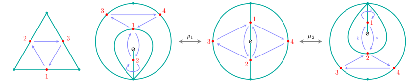
Figure 6. Quivers with 3-cycles potential associated to triangulations

A $\mathrm{T}$-triangle $T$ is self-folded if two of its edges are coincide as one $\gamma_{i}$. We call such a $\gamma_{i}$ a self-folded edge. The other edge of $T$ is call an enclosing edge.

Definition 2.9.

A puncture is called $\mathrm{T}$-isolated, if it is enclosed in a self-folded $\mathrm{T}$-triangle. Denote by $\leftmoon(\mathrm{T})$ the set of $\mathrm{T}$-isolated triangles. We say a triangulation $\mathrm{T}$ is admissible if all punctures are $\mathrm{T}$-isolated, i.e. $\leftmoon(\mathrm{T})=\text{\Sun}$.

Note that the quiver $Q_{\mathrm{T}}^{\text{\Sun}}$ has exactly $|\leftmoon(\mathrm{T})|$ loops and $|\leftmoon(\mathrm{T})|$ 2-cycles,

For any decorated triangulation $\mathbb{T}$ of $\mathbf{S}_{\Delta}^{\text{\Sun}}$, the associated quiver with potential $(Q_{\mathbb{T}},W_{\mathbb{T}})$ is defined to the one associated to $\mathrm{T}=F^{\Delta}(\mathbb{T})$ of $\mathbf{S}^{\text{\Sun}}$. Then we have the same notions of $\mathbb{T}$-isolated, $\leftmoon(\mathrm{T})$ and admissible in the decorated case.

Let $\mathbb{T}^{*}$ be the dual graph of $\mathbb{T}$ consisting of closed arcs. There is a partition $\mathbb{T}^{*}=\mathbb{T}^{*}_{\operatorname{CA}}\sqcup\mathbb{T}^{*}_{\operatorname{LA}}$ for

$$\mathbb{T}^{*}_{\operatorname{CA}}=\mathbb{T}^{*}\cap\operatorname{CA}(\mathbf{S}_{\Delta}^{\text{\Sun}})\quad\text{and}\quad\mathbb{T}^{*}_{\operatorname{LA}}=\mathbb{T}^{*}\cap\operatorname{LA}(\mathbf{S}_{\Delta}^{\text{\Sun}}).$$

Note that $\mathbb{T}^{*}_{\operatorname{LA}}$ are precisely the dual of self-folded edges in $\mathbb{T}$.

Convention 2.10.

For $Q_{\mathbb{T}}$, we will identify its vertices with (simple or L-) closed arcs.

Definition 2.11.

The mixed twist group $\operatorname{MT}(\mathbb{T})$ with respect to a triangulation $\mathbb{T}$ is defined to be the subgroup of $\operatorname{SBr}(\mathbf{S}_{\Delta})$ generated by the braid twists $\eta$ for $\eta\in\mathbb{T}^{*}_{\operatorname{CA}}$ and the L-twists $\zeta$ for $\zeta\in\mathbb{T}^{*}_{\operatorname{LA}}$.

By [QZ1, Lem. A.1], $\mathbf{S}^{\text{\Sun}}$ (and hence $\mathbf{S}_{\Delta}^{\text{\Sun}})$ admits admissible triangulations. Assume $\mathbb{T}$ is admissible. Then by cutting out all the self-folded edges in self-folded $\mathbb{T}$-triangles, we obtain a triangulation $\mathbb{T}_{0}$ for the result DMS $\mathbf{S}_{\Delta}^{0}$ without punctures. Moreover, one can naturally identify arcs in $\mathbb{T}_{\operatorname{CA}}$ and arcs in $\mathbb{T}_{0}$ as well as their dual graphs $\mathbb{T}^{*}_{\operatorname{CA}}=\mathbb{T}_{0}^{*}$.

By [QZ2, Thm. 5.9], we have a presentation of $\operatorname{BT}(\mathbf{S}_{\Delta}^{0})=\operatorname{BT}(\mathbb{T}_{0})$ with $\mathbb{T}_{0}^{*}$ as the set of generators and a set of relations, denote by $R(\mathbb{T}_{0})$, described in terms of the associated quiver with potential $(Q_{\mathbb{T}_{0}},W_{\mathbb{T}_{0}})$. Here, $(Q_{\mathbb{T}_{0}},W_{\mathbb{T}_{0}})$ is the full sub-quiver of $(Q_{\mathbb{T}},W_{\mathbb{T}})$, restricted to $Q_{\mathbb{T}_{\operatorname{CA}}}=Q_{\mathbb{T}_{0}}$ and $\operatorname{BT}(\mathbb{T}_{0})$ can be naturally embedded into $\operatorname{MT}(\mathbb{T})$ (induced from the embedding $\mathbf{S}_{\Delta}^{0}\hookrightarrow\mathbf{S}_{\Delta}^{\text{\Sun}}$.

Theorem 2.12.

Let $\mathbb{T}$ be an adimissible triangulation of $\mathbf{S}_{\Delta}^{\text{\Sun}}$ and $\mathbb{T}_{0}$ the corresponding triangulation of the surface $\mathbf{S}_{\Delta}^{0}$ cutting at the punctures in $\leftmoon(\mathbb{T})$. Then the mixed twist group $\operatorname{MT}(\mathbf{S}_{\Delta}^{\text{\Sun}})=\operatorname{MT}(\mathbb{T})$ has the following finite presentation:

• Generators:

  • generators of $\operatorname{BT}(\mathbb{T}_{0})$ (i.e. braid twists $B_{\eta}$ for $\eta\in\mathbb{T}^{*}_{\operatorname{CA}}$) together with

  • L-twists $L_{\zeta}$ for $\zeta\in\mathbb{T}^{*}_{\operatorname{LA}}$.

• Relations:

  • $R(\mathbb{T}_{0})$ for $\operatorname{BT}(\mathbb{T}_{0})$ together with

  • $\operatorname{Br}^{2\operatorname{Int}(\beta,\zeta)+2}(\beta,\zeta)$ for any $\beta\in\mathbb{T}^{*}$ and $\zeta\in\mathbb{T}^{*}_{\operatorname{LA}}$.

A special case of the theorem above is the following (when $Q_{\mathbb{T}}$ has no double arrows), where the relations are much simpler.

Corollary 2.13.

For an admissible triangulation $\mathbb{T}$ of $\mathbf{S}_{\Delta}^{\text{\Sun}}$ such that there is no double arrow in $Q_{\mathbb{T}}$, then the mixed twist group $\operatorname{MT}(\mathbf{S}_{\Delta}^{\text{\Sun}})$ has the following finite presentation:

• Generators: braid twists $\eta$ for $\eta\in\mathbb{T}^{*}_{\operatorname{CA}}$ and L-twists $\zeta$ for $\zeta\in\mathbb{T}^{*}_{\operatorname{LA}}$.

• Relations:

  • higher braid relation $\operatorname{Br}^{2\operatorname{Int}(a,b)+2}(a,b)$ for any $a,b\in\mathbb{T}^{*}$.

  • triangle relation $abca=bcab=cabc$ if $a,b,c\in\mathbb{T}^{*}_{\operatorname{CA}}$ share a common endpoint/decoration $Z$ and they are in clockwise order at $Z$.

Note that for the (higher) braid relation in Corollary 2.13, there are three cases:

• $\operatorname{Co}(a,b)$ for any $a,b\in\mathbb{T}^{*}$ with $\operatorname{Int}(a,b)=0$.

• $\operatorname{Br}(a,b)$ for any $a,b\in\mathbb{T}^{*}_{\operatorname{LA}}$ with $\operatorname{Int}(a,b)=1/2$.

• $\operatorname{Sb}(a,b)$ for $a\in\mathbb{T}^{*}_{\operatorname{CA}}$ and $b\in\mathbb{T}^{*}_{\operatorname{LA}}$ with $\operatorname{Int}(a,b)=1$.

Here $\operatorname{Int}$ is the intersection number, cf. [Qy2, Def. 3.1].

2.6. Proof of Theorem 2.12

An inductive algorithm

Lemma 2.14.

Suppose that there is a finite presentation

$$\operatorname{MT}(\mathbf{S}_{\Delta}^{\text{\Sun}\mid\leftmoon_{j}})=\frac{\langle a,\eta,x,\cdots\rangle}{\Big{(}\operatorname{Br}(\eta,x),\operatorname{Br}(a,x),\operatorname{Br}(a,x^{\eta}),\operatorname{Co}(?,a),\operatorname{Co}(?,\eta),?\neq x\Big{)}\bigcup R_{j}},$$

where $\eta,x,a$ are shown in Figure 7, the rest of the generators are disjoint with $\eta\cup a$ and any relation in $R_{j}$ does not involve $\eta$ and $a$.

Then there is a finite presentation

$$\operatorname{MT}(\mathbf{S}_{\Delta}^{\text{\Sun}\mid\leftmoon_{j+1}})=\frac{\langle\zeta,\eta,x,\cdots\rangle}{\Big{(}\operatorname{Br}^{4}(\zeta,\eta),\operatorname{Br}(\eta,x),\operatorname{Co}(x,\zeta),\operatorname{Co}(?,\zeta),\operatorname{Co}(?,\eta),?\neq x\Big{)}\bigcup R_{j}}$$ (2.21)

for some conjugation $\zeta$ of $\zeta_{j+1}$.

Proof.

We can make the (inner) semidirect product $\operatorname{MT}(\mathbf{S}_{\Delta}^{\text{\Sun}\mid\leftmoon_{j}})\rtimes_{\rho}\mathbb{Z}\langle\zeta\rangle$ that fits into the following commutative diagram of short exact sequences of groups:

(2.22)

By calculating the conjugation action of generators by $\zeta$ (denoted by $\rho_{\zeta}$), e.g.

$$\rho_{\zeta}(\eta)=a^{\prime}=a^{\underline{\eta}}\quad\text{gives relation}\quad\eta^{\zeta}=a^{\underline{\eta}},$$

we deduce that $\operatorname{MT}(\mathbf{S}_{\Delta}^{\text{\Sun}\mid\leftmoon_{j}})$ admits a presentation with generators $\langle\zeta,a,\eta,x,\cdots\rangle$ and relations

$$\Big{(}\begin{cases}\operatorname{Br}(\eta,x),\operatorname{Br}(a,x),\operatorname{Br}(a,x^{\eta}),\operatorname{Co}(?,a),\operatorname{Co}(?,\eta),?\neq x\\ a^{\zeta}=\eta,\eta^{\zeta}=a^{\underline{\eta}},x^{\zeta}=x,\operatorname{Co}(*,\zeta),*\neq\eta,a,x\end{cases}\Big{)}\bigcup R_{j}.$$ (2.23)

Here, for most conjugations by $\rho_{\zeta}$, the element $*$ (e.g. $x$) does not change so that we get $\operatorname{Co}(*,\zeta)$. By $a^{\zeta}=\eta\Leftrightarrow a=\eta^{\underline{\zeta}}$, we can eliminate $a$ from the generating set and direct calculation shows the following

$$\eta^{\zeta}=a^{\underline{\eta}}\;\Longleftrightarrow\;\underline{\zeta}\eta\zeta=\eta\eta^{\underline{\zeta}}\underline{\eta}\;\Longleftrightarrow\;\zeta\eta\zeta\eta=\eta\zeta\eta\zeta$$ (2.24)

or $\operatorname{Br}^{4}(\zeta,\eta)$ as expected. Furthermore, using these relation, we have

$$\begin{cases}\operatorname{Br}(a,x)\;\Longleftrightarrow\;\operatorname{Br}(\eta^{\underline{\zeta}},x)\;\xLongleftrightarrow{\operatorname{Co}(\zeta,x)}\;\operatorname{Br}(\eta,x)\\ \operatorname{Br}(a,x^{\eta})\;\Longleftrightarrow\;\operatorname{Br}(\eta^{\underline{\zeta}},x^{\eta})\;\Longleftrightarrow\;\operatorname{Br}(\eta^{\underline{\zeta\eta}},x)\;\xLongleftrightarrow{\operatorname{Br}^{4}(\zeta,\eta)}\;\operatorname{Br}(\eta^{\zeta},x)\;\xLongleftrightarrow{\operatorname{Co}(\zeta,x)}\;\operatorname{Br}(\eta,x).\end{cases}$$

Thus, the presentation (2.23) simplifies to (2.21). ∎

Figure 7. Presentation by extension

A first presentation for $\operatorname{MT}(\mathbf{S}_{\Delta}^{\text{\Sun}})$

We proceed to calculate presentations of the mixed twist groups $\operatorname{MT}(\mathbf{S}_{\Delta}^{\text{\Sun}\mid\leftmoon_{j}})$. We follow the notations of Figure 3 and (2.5). Set

$$\tau_{-s}=\sigma_{1}^{\zeta_{p}\cdots\zeta_{s}},\quad 1\leq s\leq p$$

to replace $\tau_{2g+b-1+s}$ for $1\leq s\leq p$. Then the relative position of these $\tau_{r}$’s is shown in the top picture of Figure 8. We recall another finite presentation in [QZ2] (with slight modification).

Theorem 2.15.

[QZ2, Thm. 4.1] Suppose that either $\aleph\geq 5$, or $\aleph=4$ and $\operatorname{rk}\leq 2$. The braid twist group $\operatorname{BT}(\mathbf{S}_{\Delta}^{\text{\Sun}})$ has the following finite presentation.

• Generators: $\sigma_{i}$ and $\tau_{r}$ for $1\leq i\leq\aleph-1,-p\leq r(\neq 0)\leq 2g+b-1$.

• Relations: the standard ones

  $$\begin{cases}\operatorname{Co}(\sigma_{i},\sigma_{j})&\text{if $|i-j|>1$}\\ \operatorname{Br}(\sigma_{i},\sigma_{j})&\text{if $|i-j|=1$}\\ \operatorname{Co}(\tau_{r},\sigma_{i})&\text{if $i>2$}\\ \operatorname{Br}(\tau_{r},x)&\forall r\\ \operatorname{Br}(\tau_{r},y)&\forall r\\ \end{cases}$$ (2.25)

  together with two extra ones

  $$\begin{cases}\operatorname{Co}({\tau_{r}}^{y},{\tau_{s}}^{x})&\text{if $r<s<0$ or $s<0<r$,}\\ \operatorname{Co}({\tau_{r}}^{y},{\tau_{s}}^{x})&\text{if $0<s<r$ and $s\in 2\mathbb{Z}^{+}_{\leq g}$,}\\ \operatorname{Co}({\tau_{r}}^{\underline{y}},{\tau_{s}}^{x})&\text{if $0<s<r$ and $s+1\in 2\mathbb{Z}^{+}_{\leq g}$,}\end{cases}$$ (2.26)

  for (cf. [QZ2, Fig. 11]

  $$x:=\tau_{-1}{}^{\underline{\sigma_{2}}}=\sigma_{2}^{\tau_{-1}},\quad y:=\sigma_{3}^{\underline{\sigma_{2}}}=\sigma_{2}^{\sigma_{3}}$$

  and any $-p\leq s,r<2g+b$ with $sr\neq 0$.

Denote by $\Sigma_{j}$ the surface obtained form $\mathbf{S}_{\Delta}^{\text{\Sun}}$ by forgetting about the punctures $\{P_{s}\mid 1\leq s\leq j\}$. Note that $\Sigma_{0}=\mathbf{S}_{\Delta}^{\text{\Sun}}$ and $\Sigma_{p}\cong\mathbf{S}_{\Delta}^{0}$ (as decorated surfaces). The braid twist group $\operatorname{BT}(\Sigma_{j})$ is a subgroup of $\operatorname{BT}(\mathbf{S}_{\Delta}^{\text{\Sun}})$ with generators

$$G_{j}=\{\sigma_{i},\tau_{r}\mid 1\leq i\leq\aleph-1,\ -p+j\leq r(\neq 0)\leq 2g+b-1\}$$ (2.27)

and same relations involving these generators. Denote the set of relations by $\Lambda_{j}$.

The relative positions of the generators in $G_{0}$ are shown in the top picture of Figure 8 and there are four kinds of them:

• $\tau_{s}$ for ${1\leq s\leq 2g}$ correspond to arcs going around the genus.

• $\tau_{s}$ for ${2g+1\leq s\leq 2g+b-1}$ correspond to arcs going around the boundary components.

• $\tau_{-s}$ for $1\leq s\leq p$ correspond to arcs going around punctures.

• $\sigma_{i}$ for ${1\leq i\leq\aleph-1}$ correspond to the ones connecting other decorations.

Figure 8. Moving the generators

Our strategy is to moving the arc $\tau_{-s}$, for $1\leq s\leq p$, so that their endpoints are separated the upper part of the top picture of Figure 8 as shown in the bottom picture there. The method of moving is by conjugation. For instance, we begin with moving $\tau_{-1}$ to $a_{1}$, by conjugating $\sigma_{2},\ldots,\sigma_{\aleph-1}$ first, then by $\tau_{-2}$ and then by $\sigma_{2},\ldots,\sigma_{\aleph-2}$. Explicitly, we have

$$a_{1}=\tau_{-1}^{\quad\underline{\left(\sigma_{2}\cdots\sigma_{\aleph-1}\right)\cdot\tau_{-2}\left(\sigma_{2}\cdots\sigma_{\aleph-2}\right)}}$$ (2.28)

The change of the relations are easy to write down accordingly as at each step we only conjugate by one of the generators. Now we apply Lemma 2.14, setting $(x,\eta,a,\zeta)=(\sigma_{\aleph-2}.\sigma_{\aleph-1},a_{1},\zeta_{1})$, to get a presentation of the mixed twist group

$$\operatorname{MT}(\mathbf{S}_{\Delta}^{\text{\Sun}\mid\leftmoon_{1}})=\langle\operatorname{MT}(\mathbf{S}_{\Delta}^{\text{\Sun}\mid\leftmoon_{0}}),\zeta_{1}\rangle=\langle\operatorname{BT}(\mathbf{S}_{\Delta}),\zeta_{1}\rangle$$

from Theorem 2.15, with the set of generators $(G_{0}\smallsetminus\{\tau_{-1}\})\cup\{\zeta_{1}\}=G_{1}\cup\{\zeta_{1}\}$. Directly calculation shows that the relations are precisely $\Lambda_{1}$ together with

$$\operatorname{Sb}(\zeta_{1},\sigma_{\aleph-1})\quad\text{and}\quad\operatorname{Co}(\zeta_{1},\alpha),\alpha\in G_{1}\smallsetminus\sigma_{\aleph-1}.$$

Now we can proceed to move next $\tau_{-s}$ and then include another $\zeta_{s}$ in $\operatorname{LA}(\mathbf{S}_{\Delta}^{\text{\Sun}})$ to get a presentation inductively for

$$\operatorname{MT}(\mathbf{S}_{\Delta}^{\text{\Sun}\mid\leftmoon_{j}})=\langle\operatorname{MT}(\mathbf{S}_{\Delta}^{\text{\Sun}\mid\leftmoon_{j-1}}),\zeta_{j}\rangle.$$ (2.29)

Note that in order to apply Lemma 2.14 properly, we need to move $\sigma_{\aleph-s}$ a bit, e.g. by conjugating $\underline{\sigma_{\aleph-s-1}\sigma_{\aleph-s-2}}$ (and move back afterward). Similarly as above, the set of generators is $\{\zeta_{s}\mid 1\leq s\leq j\}\cup G_{j}$, for the L-twist along some L-arcs $\zeta_{s}$, and the relations are precisely $\Lambda_{j}$ together with

$$\operatorname{Sb}(\zeta_{s},\beta_{s})\quad\text{and}\quad\operatorname{Co}(\zeta_{s},\alpha),\alpha\in G_{j}\smallsetminus\beta_{s};\quad 1\leq s\leq j,$$

where $\beta_{s}$ is the only arc in $G_{j}$ that intersect with $\zeta_{s}$ (and with $\operatorname{Int}=1$).

Equivalence between presentations

For $s=p$, we obtain a presentation for $\operatorname{MT}(\mathbf{S}_{\Delta}^{\text{\Sun}})$, which compares with the presentation of $\operatorname{BT}(\Sigma_{p})=\operatorname{BT}(\mathbf{S}_{\Delta})$, the set of generators has extra $p$ L-twists $\{\zeta_{s}\mid 1\leq s\leq p\}$, the set of relations has extra relations:

$$\operatorname{Sb}(\zeta_{s},\beta_{s})\quad\text{and}\quad\operatorname{Co}(\zeta_{s},\alpha),\alpha\in G_{j}\smallsetminus\beta_{s};\quad 1\leq s\leq p.$$

Since $\mathbf{S}_{\Delta}\cong\mathbf{S}_{\Delta}^{0}$ as decorated surfaces, we have $\operatorname{BT}(\mathbf{S}_{\Delta})\cong\operatorname{BT}(\mathbf{S}_{\Delta}^{0})=\operatorname{BT}(\mathrm{T}_{0}^{*})=\operatorname{BT}(\mathbb{T}^{*}_{\operatorname{CA}})$. As shown in [QZ2], the presentation of $\operatorname{BT}(\mathrm{T}_{0}^{*})$ is in fact derived from $\operatorname{BT}(\mathbf{S}_{\Delta})$. Thus, the above presentation is equivalent to the one in Theorem 2.12. ∎

3. Flip graphs and categorification

3.1. Flip (exchange) graphs

Let $\mathrm{T}$ be a triangulation of $\mathbf{S}$. For any $\gamma$ in $\mathrm{T}$, the neighbourhood $N_{\mathrm{T}}(\gamma)$ of $\gamma$ are the union of all $\mathrm{T}$-triangles containing $\gamma$. If $\gamma$ is not a self-folded edge, there are exactly two $\mathrm{T}$-triangles containing $\gamma$ and $N_{\mathrm{T}}(\gamma)$ is a quadrilateral. If $\gamma$ is a self-folded edge in $\mathrm{T}$, then $N_{\mathrm{T}}(\gamma)$ is a self-folded triangle but still can be treated as quadrilateral with two edges gluing together.

At each non self-folded edge $\gamma$ of $\mathrm{T}$, there is an operation $\mu_{\gamma}\colon\mathrm{T}-\mathrm{T}^{\prime}$, known as the usual (unoriented) flip with respect to $\gamma$, which produces another triangulation $\mathrm{T}^{\prime}$ from $\mathrm{T}$ by replacing the diagonal $\gamma$ of $N_{\mathrm{T}}(\gamma)$ by the unique other diagonal $\gamma^{\prime}$ of $N_{\mathrm{T}}(\gamma)$.

Denote by $\underline{\operatorname{EG}}(\mathbf{S}^{\text{\Sun}})$ the unoriented exchange graph of triangulations of $\mathbf{S}^{\text{\Sun}}$, whose vertices are triangulations and whose edges are usual flips. The following is a well-known fact, cf. [Hat, Har] or [FST, Thm. 3.10].

Theorem 3.1.

$\underline{\operatorname{EG}}(\mathbf{S}^{\text{\Sun}})$ is connected and its fundamental group is generated by (unoriented) squares and pentagons, locally looks like the left and middle pictures of Figure 11 (forgetting about the orientations of edges and the decorations there).

There is an oriented version of $\underline{\operatorname{EG}}(\mathbf{S}^{\text{\Sun}})$.

Definition 3.2.

Let $\mathrm{T}$ be a triangulation of $\mathbf{S}^{\text{\Sun}}$ and $\gamma$ be an open arc in $\mathrm{T}$. There is an operation $\mu^{\sharp}_{\gamma}\colon\mathrm{T}\to\mathrm{T}^{\sharp}_{\gamma}$, known as the forward flip with respect to $\gamma$, which produces another triangulation $\mathrm{T}^{\sharp}_{\gamma}$ from $\mathrm{T}$ by replacing the arc $\gamma$ with $\gamma^{\sharp}$. Here, $\gamma^{\sharp}$ is the open arc obtained from $\gamma$ by moving each of its endpoint, anticlockwise along boundaries of $N_{\mathrm{T}}(\gamma)$ to the next marked point or puncture.

The forward flip operation also applies to decorated triangulations of $\mathbf{S}_{\Delta}^{\text{\Sun}}$. The inverse operation of which is the backward flip, denoted by $\mu^{\flat}_{\gamma}=(\mu^{\sharp}_{\gamma})^{-1}$. We will use the notation $\pm\sharp=\mp\flat$ from now on.

The three possible cases of forward flips are shown in Figure 9, for both $\mathbf{S}_{\Delta}^{\text{\Sun}}$ and $\mathbf{S}^{\text{\Sun}}$ with vertical correspondence by forgetful map. The first two are usual forward flips and the last one (on the right) is the self-folded forward flip or forward L-flip for short.

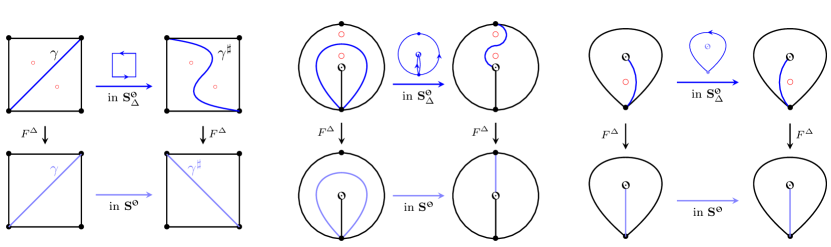
Figure 9. The forward flips with forgetful map

Denote by $\operatorname{FG}(\mathbf{S}^{\text{\Sun}})$ and $\operatorname{FG}(\mathbf{S}_{\Delta}^{\text{\Sun}})$ the flip (exchange) graph of (decorated) triangulations of $\mathbf{S}^{\text{\Sun}}$ and $\mathbf{S}_{\Delta}^{\text{\Sun}}$, respectively, where oriented edges are forward flips. We use $\operatorname{FG}$ instead of $\operatorname{EG}$ to distinguish with the various other exchange graphs.

Figure 10. Cluster exchange graph V.S. flip graph for once-punctured triangle

Example 3.3.

If $\mathbf{S}^{\text{\Sun}}$ is a once punctured triangle, then $\underline{\operatorname{EG}}(\mathbf{S}^{\text{\Sun}})$ and $\operatorname{FG}(\mathbf{S}^{\text{\Sun}})$ are shown in the right picture of Figure 10, where the unoriented/oriented version is in gray/purple, respectively.

Remark 3.4.

When there is no punctures, $\operatorname{FG}(\mathbf{S}^{\text{\Sun}})$ can be obtained from $\underline{\operatorname{EG}}(\mathbf{S}^{\text{\Sun}})$ by replacing each unoriented edge with a 2-cycle, as we did in [KQ2]. However, with punctures, $\underline{\operatorname{EG}}(\mathbf{S}^{\text{\Sun}})$ is not $n$-regular (i.e. there are $n$ edges at each vertex). We fix this by including forward L-flip, which is a loop in $\operatorname{FG}(\mathbf{S}^{\text{\Sun}})$, so that $\operatorname{FG}(\mathbf{S}^{\text{\Sun}})$ is still $(n,n)$-regular (i.e. there are $n$ edges going out and in, respectively, at each vertex). Moreover, one can obtained $\underline{\operatorname{EG}}(\mathbf{S}^{\text{\Sun}})$ from $\operatorname{FG}(\mathbf{S}^{\text{\Sun}})$ by deleting loop edges and replacing every 2-cycle by an unoriented edge.

In Appendix B, we will study the flip exchange graph with cluster style tagging at some of the punctures. For instance, the left picture of Figure 10 is the cluster exchange graph associated to $\mathbf{S}^{\text{\Sun}}$ (the famous associahedron).

As in the undecorated case, there a natural covering.

Lemma 3.5.

The forgetful map induces a Galois covering $F^{\Delta}_{*}:\operatorname{FG}(\mathbf{S}_{\Delta}^{\text{\Sun}})\to\operatorname{FG}(\mathbf{S}^{\text{\Sun}})$ with covering group $\operatorname{SBr}(\mathbf{S}_{\Delta}^{\text{\Sun}})$.

Proof.

Notice that although some of the edges are loops, the two graphs are both $(n,n)$-regular. The rest follows the same as [KQ2, Lem. 3.8]. ∎

Usually, $\operatorname{FG}(\mathbf{S}_{\Delta}^{\text{\Sun}})$ is not connected. The more tricky business is to determine the covering group when restricted to a connected component. In the unpunctured case, this is stated properly as [BMQS, Thm. 4.8], cf [Qy2, Rem. 3.10]. In the punctured case, it is even harder (as the cluster theory is not applicable).

Fix any $\mathbb{T}\in\operatorname{FG}(\mathbf{S}_{\Delta}^{\text{\Sun}})$. Denote by $\operatorname{FG}^{\mathbb{T}}(\mathbf{S}_{\Delta}^{\text{\Sun}})$ the connected component of $\operatorname{FG}(\mathbf{S}_{\Delta}^{\text{\Sun}})$ containing $\mathbb{T}$. So there is a covering

$$F^{\Delta}_{*}\mid_{\mathbb{T}}\colon\operatorname{FG}^{\mathbb{T}}(\mathbf{S}_{\Delta}^{\text{\Sun}})\to\operatorname{FG}(\mathbf{S}^{\text{\Sun}}),$$ (3.1)

whose covering group is denoted by $\operatorname{MT}^{\text{\Sun}}\leq\operatorname{SBr}(\mathbf{S}_{\Delta}^{\text{\Sun}})$. We will show that $\operatorname{MT}^{\text{\Sun}}$ is in fact $\operatorname{MT}(\mathbf{S}_{\Delta}^{\text{\Sun}})$, which implies the following (using Theorem 2.6).

Corollary 3.6.

The connected components of $\operatorname{FG}(\mathbf{S}_{\Delta}^{\text{\Sun}})$ is parameterized by

$$\operatorname{SBr}(\mathbf{S}_{\Delta}^{\text{\Sun}})/\operatorname{MT}(\mathbf{S}_{\Delta}^{\text{\Sun}})\cong\operatorname{\bf H}_{1}(\mathbf{S}).$$

3.2. The 3-Calabi-Yau category $\operatorname{\mathcal{D}}_{3}(\mathbf{S}_{\Delta}^{\text{\Sun}})$

Recall that we assume that (2.20) which ensures that $\mathbf{S}_{\Delta}^{\text{\Sun}}$ admits decorated triangulations. We will fix a triangulation $\mathbb{T}$, which induces a natural grading on $\mathbf{S}_{\Delta}^{\text{\Sun}}$ induced by $\mathbb{T}$, cf. [CHQ, § 2] for more details. Note that any triangulation and the dual graph of which carries natural gradings. Denote by $\widetilde{\operatorname{CA}}(\mathbf{S}_{\Delta}^{\text{\Sun}})$ the set of graded arcs whose underlying arcs are in $\operatorname{CA}(\mathbf{S}_{\Delta}^{\text{\Sun}})$. Similarly for $\widetilde{\operatorname{LA}}(\mathbf{S}_{\Delta}^{\text{\Sun}})$ or a graded arc $\widetilde{\alpha}$.

For the preliminaries on simple tilting theory, see Section A.1.

Let $\Gamma_{\mathbb{T}}^{\text{\Sun}}=\Gamma(Q_{\mathbb{T}}^{\text{\Sun}},W_{\mathbb{T}}^{\text{\Sun}})$ be the Ginzburg algebra associated to the quiver with potential $(Q_{\mathbb{T}}^{\text{\Sun}},W_{\mathbb{T}}^{\text{\Sun}})$ and $\operatorname{\mathcal{D}}_{3}(\mathbf{S}_{\Delta}^{\text{\Sun}})$ the perfectly valued (or finite dimensional) derived category of $\Gamma_{\mathbb{T}}^{\text{\Sun}}$.

The following is well-known (cf. [Ke1]): $\operatorname{\mathcal{D}}_{3}(\mathbf{S}_{\Delta}^{\text{\Sun}})$ is 3-Calabi-Yau with a canonical heart $\operatorname{\mathcal{H}}_{\mathbb{T}}^{\text{\Sun}}$ being (dg) module category of $\Gamma_{\mathbb{T}}^{\text{\Sun}}$. Denote by $\operatorname{Sph}\operatorname{\mathcal{D}}_{3}(\mathbf{S}_{\Delta}^{\text{\Sun}})$ the set of (reachable) spherical objects in $\operatorname{\mathcal{D}}_{3}(\mathbf{S}_{\Delta}^{\text{\Sun}})$ and $\operatorname{EG}^{\mathbb{T}}(\operatorname{\mathcal{D}}_{3}(\mathbf{S}_{\Delta}^{\text{\Sun}}))$ the principal component of exchange graph of hearts of $\operatorname{\mathcal{D}}_{3}(\mathbf{S}_{\Delta}^{\text{\Sun}})$. Here is a summery of the results in [Chr, CHQ], specified to our category.

Theorem 3.7.

[CHQ] There is an injective map:

$$\begin{array}[]{rcl}\operatorname{X}^{\text{\Sun}}\colon\widetilde{\operatorname{CA}}(\mathbf{S}_{\Delta}^{\text{\Sun}})\bigsqcup\widetilde{\operatorname{LA}}(\mathbf{S}_{\Delta}^{\text{\Sun}})&\to&\operatorname{Obj}\operatorname{\mathcal{D}}_{3}(\mathbf{S}_{\Delta}^{\text{\Sun}}),\\ \widetilde{\alpha}&\mapsto&\operatorname{X}^{\text{\Sun}}_{\widetilde{\alpha}},\end{array}$$ (3.2)

satisfying

$$\operatorname{Int}^{d}(\widetilde{\alpha},\widetilde{\beta})=\dim\operatorname{Hom}^{d}(\operatorname{X}^{\text{\Sun}}_{\widetilde{\alpha}},\operatorname{X}^{\text{\Sun}}_{\widetilde{\beta}}).$$ (3.3)

Moreover, $\operatorname{X}^{\text{\Sun}}$ induces an isomorphism of oriented graphs:

$$\begin{array}[]{rcl}\operatorname{X}^{\text{\Sun}}_{*}\colon\operatorname{FG}^{\mathbb{T}}(\mathbf{S}_{\Delta}^{\text{\Sun}})&\xrightarrow{\cong}&\operatorname{EG}^{\mathbb{T}}(\operatorname{\mathcal{D}}_{3}(\mathbf{S}_{\Delta}^{\text{\Sun}})),\\ \mathbb{T}&\mapsto&\operatorname{\mathcal{H}}_{\mathbb{T}}^{\text{\Sun}},\\ \end{array}$$ (3.4)

such that $\operatorname{Sim}\operatorname{\mathcal{H}}_{\mathbb{T}}^{\text{\Sun}}=\operatorname{X}^{\text{\Sun}}(\widetilde{\mathbb{T}^{*}})$.

In particular, for $\widetilde{\zeta}\in\widetilde{\operatorname{LA}}(\mathbf{S}_{\Delta}^{\text{\Sun}})$, $\operatorname{Ext}^{1}(\operatorname{X}^{\text{\Sun}}_{\widetilde{\zeta}},\operatorname{X}^{\text{\Sun}}_{\widetilde{\zeta}})=\mathbf{k}$ and when restricted to $\widetilde{\operatorname{CA}}(\mathbf{S}_{\Delta}^{\text{\Sun}})$, one has an injection

$$\begin{array}[]{rcl}\operatorname{X}^{\text{\Sun}}\colon\widetilde{\operatorname{CA}}(\mathbf{S}_{\Delta}^{\text{\Sun}})&\xrightarrow{1-1}&\operatorname{Sph}^{\circ}(\operatorname{\mathcal{D}}_{3}(\mathbf{S}_{\Delta}^{\text{\Sun}})),\\ \widetilde{\eta}&\mapsto&\operatorname{X}^{\text{\Sun}}_{\widetilde{\eta}},\end{array}$$ (3.5)

Thus, $\operatorname{X}^{\text{\Sun}}_{\widetilde{\alpha}}$ is rigid if and only if $\alpha$ is in $\operatorname{CA}(\mathbf{S}_{\Delta}^{\text{\Sun}})$.

Denote by $\operatorname{FG}_{\text{\tiny{$\copyright$}}}(\mathbf{S}_{\Delta}^{\text{\Sun}})$ the subgraph of $\operatorname{FG}(\mathbf{S}_{\Delta}^{\text{\Sun}})$ by deleting all L-flip edges. Equivalently, it consists of flips $\mu^{\sharp}_{\gamma}:\mathbb{T}\to\mathbb{T}^{\sharp}$ such that the dual closed arc of the flipped open arc $\gamma$ is in $\operatorname{CA}(\mathbf{S}_{\Delta}^{\text{\Sun}})$ (not in $\operatorname{LA}(\mathbf{S}_{\Delta}^{\text{\Sun}})$). Similarly for other variation of $\operatorname{FG}_{\text{\tiny{$\copyright$}}}$. We get the following corollary.

Corollary 3.8.

The isomorphism $\operatorname{X}^{\text{\Sun}}_{*}$ in (3.4) restricts to an isomorphism

$$\operatorname{X}^{\text{\Sun}}_{*}\colon\operatorname{FG}_{\text{\tiny{$\copyright$}}}^{\circ}(\mathbf{S}_{\Delta}^{\text{\Sun}})\xrightarrow{\cong}\operatorname{EG}_{\circledR}^{\circ}(\operatorname{\mathcal{D}}_{3}(\mathbf{S}_{\Delta}^{\text{\Sun}})).$$ (3.6)

Note that for any $\mathbb{T}\in\operatorname{FG}_{\text{\tiny{$\copyright$}}}(\mathbf{S}_{\Delta}^{\text{\Sun}})$, there are exactly $\#\mathbb{T}^{*}_{\operatorname{CA}}$ edges coming in and going out.

Two of the key features of the categorical side are

• the symmetry triangulated shift $[1]$ and

• the natural partial order on hearts.

Under the correspondences in Theorem 3.7, we can also use $[1]$ and $\leq$ on the topological side for decorated triangulations of $\mathbf{S}_{\Delta}^{\text{\Sun}}$.

Remark 3.9.

For closed arcs, the shift correspond to grading shift. The map $X$ also extends to open arc and the alternative version of (3.4) is that $X(\mathbb{T})$ is in fact a silting set in the perfect derived category $\operatorname{per}(\mathbf{S}_{\Delta}^{\text{\Sun}})$, which is the Koszul dual of $\operatorname{\mathcal{H}}_{\mathbb{T}}^{\text{\Sun}}$ in $\operatorname{\mathcal{D}}_{3}(\mathbf{S}_{\Delta}^{\text{\Sun}})$. See [Qy3, Chr, CHQ] for more discussion.

On open arcs, the shift corresponds to the universal rotation $\widetilde{\rho}\in\operatorname{MCG}(\mathbf{S}_{\Delta}^{\text{\Sun}})$. More precisely, for any boundary component $\partial\in\partial\mathbf{S}_{\Delta}^{\text{\Sun}}$, there is a rotation/operation $\rho_{\partial}$ that moves each marked point to the next consecutive one:

These rotations are roots of the Dehn twists, i.e. $\rho_{\partial}^{m_{\partial}}=\operatorname{D}_{\partial}$. And the universal rotation is the product of all:

$$\widetilde{\rho}\colon=\prod_{\partial\subset\partial\mathbf{S}_{\Delta}^{\text{\Sun}}}\rho_{\partial}.$$ (3.7)

In particular, we have

$$\widetilde{\rho}\big{(}X(\mathbb{T})\big{)}=X(\mathbb{T})[1].$$

Notice that in each thin dumbbell/symmetric hexagon in (14), the source triangulated digon is the universal rotation of the sink triangulated digon.

3.3. The fundamental domain

Denote by $\operatorname{EG}_{\circledR}^{\circ}[\operatorname{\mathcal{H}}_{0},\operatorname{\mathcal{H}}_{0}[1]]$ the connected component in $\operatorname{EG}_{\circledR}[\operatorname{\mathcal{H}}_{0},\operatorname{\mathcal{H}}_{0}[1]]$ containing $\operatorname{\mathcal{H}}_{0}$. By the isomorphism (3.4), we have

$$\operatorname{FG}_{\text{\tiny{$\copyright$}}}^{\circ}[\mathbb{T}_{0},\mathbb{T}_{0}[1]]=(\operatorname{X}^{\text{\Sun}}_{*})^{-1}(\operatorname{EG}_{\circledR}^{\circ}[\operatorname{\mathcal{H}}_{0},\operatorname{\mathcal{H}}_{0}[1]])$$

for $\mathbb{T}_{0}=(\operatorname{X}^{\text{\Sun}}_{*})^{-1}(\operatorname{\mathcal{H}}_{0})$.

Denote by $\overline{\operatorname{FG}_{\text{\tiny{$\copyright$}}}^{\circ}[\mathbb{T}_{0},\mathbb{T}_{0}[1]]}^{\circlearrowleft}$ the graph obtained from $\operatorname{FG}_{\text{\tiny{$\copyright$}}}^{\circ}[\mathbb{T}_{0},\mathbb{T}_{0}[1]]$ by adding a reverse edge for each of its edges and adding $\#(\mathbb{T}^{\prime})^{*}_{\operatorname{LA}}=\#\leftmoon(\mathbb{T}^{\prime})$ loops at each vertex $\mathbb{T}^{\prime}$.

Theorem 3.10.

Suppose that $\mathbb{T}_{0}$ is admissible. Then there is a natural isomorphism

$$\operatorname{FG}^{\mathbb{T}}(\mathbf{S}_{\Delta}^{\text{\Sun}})/\operatorname{MT}(\mathbf{S}_{\Delta}^{\text{\Sun}})\cong\overline{\operatorname{FG}_{\text{\tiny{$\copyright$}}}^{\circ}[\mathbb{T}_{0},\mathbb{T}_{0}[1]]}^{\circlearrowleft}.$$ (3.8)

Proof.

Firstly, we claim that $\operatorname{MT}(\mathbf{S}_{\Delta}^{\text{\Sun}})\cdot\operatorname{FG}_{\text{\tiny{$\copyright$}}}^{\circ}[\mathbb{T}_{0},\mathbb{T}_{0}[1]]\subset\operatorname{FG}^{\mathbb{T}}(\mathbf{S}_{\Delta}^{\text{\Sun}})$. This is because the braid twist/L-twist $\operatorname{MT}(\mathbf{S}_{\Delta}^{\text{\Sun}})$ can be realized as either a composition of flips or a flip on its own. More precisely, for any $\mathbb{T}^{\prime}\in\operatorname{FG}(\mathbf{S}_{\Delta}^{\text{\Sun}})$, one has (cf. $u^{2}$ and $s$ in Figure 14, respectively)

$$(\mathbb{T}^{\prime})_{\gamma}^{\pm 2\sharp}=B_{\eta}^{\mp}(\mathbb{T}^{\prime}),$$ (3.9)

$$(\mathbb{T}^{\prime})_{\gamma}^{\pm\sharp}=L_{\zeta}^{\mp}(\mathbb{T}^{\prime}).$$ (3.10)

Here, $\eta$ or $\zeta$ in $(\mathbb{T}^{\prime})^{*}$ is the dual of the arc $\gamma\in\mathbb{T}^{\prime}$ and $(-)^{\pm 2\sharp}$ means the iterated flips. Then one can write down explicitly that the twist $\Psi(T_{0})$ can be expressed as a sequence of flips staring from $T_{0}$ in the same way as the formula [KQ1, (8.4)], for any $\Psi\in\operatorname{MT}(\mathbb{T}_{0})=\operatorname{MT}(\mathbf{S}_{\Delta}^{\text{\Sun}})$.

Secondly, we claim that $\operatorname{MT}(\mathbf{S}_{\Delta}^{\text{\Sun}})\cdot\operatorname{FG}_{\text{\tiny{$\copyright$}}}^{\circ}[\mathbb{T}_{0},\mathbb{T}_{0}[1]]\supset\operatorname{FG}^{\mathbb{T}}(\mathbf{S}_{\Delta}^{\text{\Sun}})$. We only need to how that if $\mathbb{T}^{\prime}=\Xi(\mathbb{T}_{1})$ is in $\operatorname{MT}(\mathbf{S}_{\Delta}^{\text{\Sun}})\cdot\operatorname{FG}_{\text{\tiny{$\copyright$}}}^{\circ}[\mathbb{T}_{0},\mathbb{T}_{0}[1]]$ for $\Xi\in\operatorname{MT}(\mathbf{S}_{\Delta}^{\text{\Sun}})$ and $\mathbb{T}_{1}\in\operatorname{FG}_{\text{\tiny{$\copyright$}}}^{\circ}[\mathbb{T}_{0},\mathbb{T}_{0}[1]]$, then so are the any flips of $\mathbb{T}^{\prime}$.

Equivalently, we only need to show that any flips of $\mathbb{T}_{1}$ are still in $\operatorname{MT}(\mathbf{S}_{\Delta}^{\text{\Sun}})\cdot\operatorname{FG}_{\text{\tiny{$\copyright$}}}^{\circ}[\mathbb{T}_{0},\mathbb{T}_{0}[1]]$ if $\mathbb{T}_{1}$ is. This follows as below:

• For any $\eta\in(\mathbb{T}_{1})^{*}_{\operatorname{CA}}$ with $\gamma=\eta^{*}\in\mathbb{T}_{1}$, exactly one of the flips $(\mathbb{T}_{1})^{\pm\sharp}_{\gamma}$ is in $\operatorname{FG}_{\text{\tiny{$\copyright$}}}^{\circ}[\mathbb{T}_{0},\mathbb{T}_{0}[1]]$ by Lemma A.2 (via the identification (3.6)). The other flip will be one of the braid twist $B_{\eta}^{\pm}$ of which by formula (3.9).

• For any $\zeta\in\mathbb{T}^{*}_{\operatorname{LA}}$ with $\gamma=\eta^{*}\in\mathbb{T}_{1}$, the flips $(\mathbb{T}_{1})^{\pm\sharp}_{\gamma}$ are precisely the L-twists by (3.10).

Hence $\operatorname{MT}(\mathbf{S}_{\Delta}^{\text{\Sun}})\cdot\operatorname{FG}_{\text{\tiny{$\copyright$}}}^{\circ}[\mathbb{T}_{0},\mathbb{T}_{0}[1]]=\operatorname{FG}^{\mathbb{T}}(\mathbf{S}_{\Delta}^{\text{\Sun}})$ as sets.

Finally, the formulae (3.9) implies that each edge in $\operatorname{FG}^{\mathbb{T}}(\mathbf{S}_{\Delta}^{\text{\Sun}})$ needs to be doubled and (3.10) implies that there are certain loops need to be added, so that one matches $\overline{\operatorname{FG}_{\text{\tiny{$\copyright$}}}^{\circ}[\mathbb{T}_{0},\mathbb{T}_{0}[1]]}^{\circlearrowleft}$ with $\operatorname{MT}(\mathbf{S}_{\Delta}^{\text{\Sun}})$ precisely as graphs. ∎

Recall that there is a covering (3.1) so that

$$\operatorname{FG}^{\mathbb{T}}(\mathbf{S}_{\Delta}^{\text{\Sun}})/\operatorname{MT}^{\text{\Sun}}=\operatorname{FG}(\mathbf{S}^{\text{\Sun}}).$$ (3.11)

More precisely, $\operatorname{MT}^{\text{\Sun}}$ is the subgroup of $\operatorname{SBr}(\mathbf{S}_{\Delta}^{\text{\Sun}})$ consisting of elements $f\in\operatorname{SBr}(\mathbf{S}_{\Delta}^{\text{\Sun}})$ satisfying $f(\mathbb{T})\in\operatorname{FG}^{\mathbb{T}}(\mathbf{S}_{\Delta}^{\text{\Sun}})$. Thus, $\operatorname{MT}(\mathbf{S}_{\Delta}^{\text{\Sun}})\leq\operatorname{MT}^{\text{\Sun}}$ and, by the conjugation formula (2.3), $\operatorname{MT}(\mathbf{S}_{\Delta}^{\text{\Sun}})\lhd\operatorname{MT}^{\text{\Sun}}$. But at the moment, we only have the following commutative diagram,

(3.12)

for any admissible $\mathbb{T}_{0}$, where $\operatorname{Ni}=\operatorname{MT}^{\text{\Sun}}/\operatorname{MT}(\mathbf{S}_{\Delta}^{\text{\Sun}})$.

In Section 5.2, we will show that $\operatorname{MT}^{\text{\Sun}}=\operatorname{MT}(\mathbf{S}_{\Delta}^{\text{\Sun}})$ and $\operatorname{FG}(\mathbf{S}^{\text{\Sun}})=\overline{\operatorname{FG}_{\text{\tiny{$\copyright$}}}^{\circ}[\mathbb{T}_{0},\mathbb{T}_{0}[1]]}^{\circlearrowleft}$.

4. Flip groupoids and flip twist groups

In [KQ2], we introduce the cluster exchange groupoids as the enhancement of cluster exchange graphs, using the cluster combinatorics to produce generalization of braid groups. Naturally, in the unpunctured surface case, as well as Dynkin case, we identified cluster braid groups with braid twist groups and spherical twist groups.

In this section, we introduce the flip groupoids as refinements of Cayley graphs of mixed twist groups, with the same natural above. However, the square/pentagon/dumbbell relations there are not enough here. New phenomenon appears due to the loop edges in $\operatorname{FG}(\mathbf{S}^{\text{\Sun}})$.

4.1. Relations in cluster exchange graphs

Classical Square and Pentagon (relations)

Given a triangulation $\mathrm{T}$ in $\operatorname{FG}(\mathbf{S}^{\text{\Sun}})$ with any two vertices $i,j\in Q_{\mathrm{T}}$, there is the following local full subgraph in $\operatorname{FG}(\mathbf{S}^{\text{\Sun}})$:

$$\leavevmode\hbox to145.11pt{\vbox to42.68pt{\text{[drawing]}}}. \mathrm{T}^{\prime} \bullet \bullet \mathrm{T} i j j x y x y x y \mathrm{T}^{\prime} \bullet \bullet \mathrm{T} i j j x y x y x y$$ (4.1)

Suppose that there is no arrow from $i$ to $j$. If there is at most one arrow from $j$ to $i$ in $Q_{\mathrm{T}}$, then such a subgraph completes into a double square or a double pentagon, depending on if the numbers of arrow is zero or one, as shown below.

(4.2)

The square/pentgon relation (at $\mathrm{T}$ with respect to $i,j$) is the relations $x^{2}=y^{h}$ staring at $\mathrm{T}$ (where $h=2$ for square and $h=3$ for pentagon). In fact, by the symmetry, all $x^{2}=y^{h}$ are this type of relations.

Note that these relations are well-known, cf. [Kra, Qy1]. They are not exactly the ones in Theorem 3.1, but the oriented version.

  

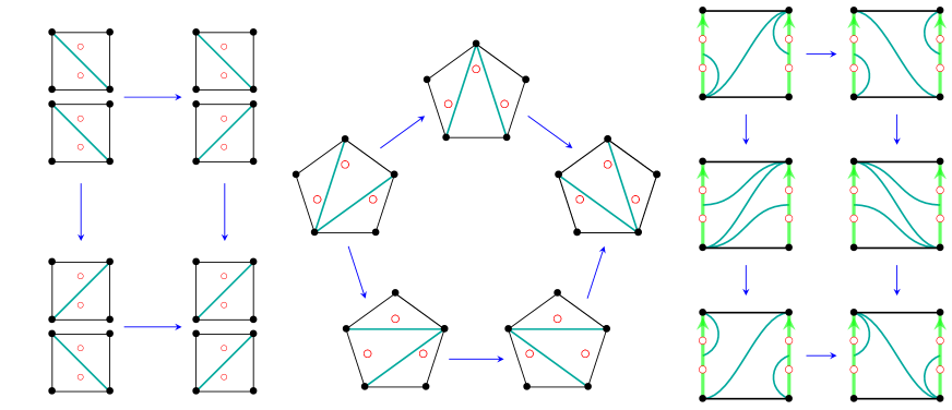
Figure 11. Square/Pentagon and Fat Dumbbell relations in $\operatorname{FG}(\mathbf{S}_{\Delta}^{\text{\Sun}})$

Original Fat Dumbbell relations (Fat-DB)

[KQ2, § 2]

Given a triangulation $\mathrm{T}$ in $\operatorname{FG}(\mathbf{S}^{\text{\Sun}})$ with two vertices $i,j$ in $Q_{\mathrm{T}}$ such that the corresponding open arcs in $\mathrm{T}$ are not self-folded edges. Suppose that there is no arrow from $i$ to $j$ as above and we still have (4.1). We name the edges/flips $x$ and $y$ (omitting the subscripts for simplicity). When there are arrows in one direction (between $i$ and $j$), then $x$ and $y$ can be distinguished as being forward mutation at either the tail or head of arrows.

$$\leavevmode\hbox to145.11pt{\vbox to59.75pt{\text{[drawing]}}}. \bullet \bullet \bullet \bullet \mathrm{T} x x x x y y \bullet \bullet \bullet \bullet \mathrm{T} x x x x y y$$ (4.3)

The fat dumbbell relation (at $\mathrm{T}$ with respect to $i,j$) is the hexagonal relations shown in (4.3), or $x^{2}y=yx^{2}$ staring at $\mathrm{T}$. Let $t_{i}=yx$ and $t_{j}=xy$ be the flip twists (i.e. 2-cycle) at $\mathrm{T}$ and $\mathrm{T}^{\prime}$, respectively. Then the relation can be written as conjugation relation $t_{j}=t_{i}^{x}$.

4.2. New dumbbell/hexagon relations

Thin Dumbbell relations (Thin-DB)

Figure 12. $\operatorname{FG}(\mathbf{S}^{\text{\Sun}})$ for a once-punctured digon as local flip graph

Given a triangulation $\mathrm{T}$ in $\operatorname{FG}(\mathbf{S}^{\text{\Sun}})$ with two vertices $i,j$ in $Q_{\mathrm{T}}$ such that they are in a digon as shown in the middle picture of Figure 12. They there is a full subgraph of $\operatorname{FG}(\mathbf{S}^{\text{\Sun}})$ as shown there. We name three triangulations $\mathrm{T}_{L},\mathrm{T}_{M}$ and $\mathrm{T}_{R}$, respectively (cf. Figure 12 and the third picture of Figure 13). We also name usual flips/edges $u,v$ and L-flips/loop edges $s,r$ as shown there, where the color matches the open arc that they flip at.

The thin dumbbell relations (at $\mathrm{T}_{M}$ with respect to $i,j$) are

• $r=s^{uv}$ ($\Leftrightarrow suv=uvr$) at $\mathrm{T}_{L}$ and

• $s=r^{vu}$ ($\Leftrightarrow vus=rvu$) at $\mathrm{T}_{R}$,

as shown in the left two picture of Figure 13.

Figure 13. Two thin dumbbell relations and the symmetric hexagon relations

Symmetry Hexagon (Dumbbell) relations (Sym-Hex)

Continue the set up as above (for thin dumbbell relation).

The symmetry hexagon relations (at $\mathrm{T}_{M}$ with respect to $i,j$) is $usu=vrv$, as shown in the right picture of Figure 13. Note that they will also play a role in the conjugation formula later. Thus, they are also sort of dumbbell type relations.

Definition 4.1.

The flip groupoid $\operatorname{\mathcal{FG}}(\mathbf{S}^{\text{\Sun}})$ is the quotient of the path groupoid of $\operatorname{FG}(\mathbf{S}^{\text{\Sun}})$ by all (square/pentagon, symmetry hexagon and fat/thin dumbbell) relations above.

The definition is also appeared in the parallel joint work [HKQ].

4.3. Covering groupoids

Similar to $\operatorname{\mathcal{FG}}(\mathbf{S}^{\text{\Sun}})$, we have the groupoid version of $\operatorname{FG}(\mathbf{S}_{\Delta}^{\text{\Sun}})$.

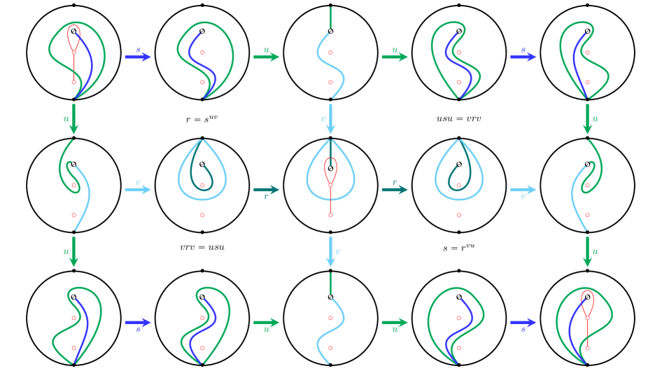
Figure 14. Higher braid relation $\eta\delta\eta\delta=\delta\eta\delta\eta$ decomposes into 4 hexagons

Definition 4.2.

There are the following lifts in $\operatorname{FG}(\mathbf{S}_{\Delta}^{\text{\Sun}})$:

• A square is shown in the left picture of Figure 11.

• A pentagon is shown in the middle picture of Figure 11.

• A Fat-DB is shown in the right picture of Figure 11.

• Two Thin-DB (relations) are shown as the top-left/bottom-right hexagons in Figure 14.

• Two Sym-Hex (relations) are shown as the top-right/bottom-left hexagons in Figure 14.

The flip groupoid $\operatorname{\mathcal{FG}}(\mathbf{S}_{\Delta}^{\text{\Sun}})$ is the quotient of the path groupoid of $\operatorname{FG}(\mathbf{S}_{\Delta}^{\text{\Sun}})$ by the five kinds of relations above.

As the relations in $\operatorname{\mathcal{FG}}(\mathbf{S}^{\text{\Sun}})$ lifts to relations in $\operatorname{\mathcal{FG}}(\mathbf{S}_{\Delta}^{\text{\Sun}})$, the isomorphism in Theorem 3.10 upgrades to an isomorphism between groupoids:

$$F^{\Delta}_{*}\colon\operatorname{\mathcal{FG}}^{\mathbb{T}}(\mathbf{S}_{\Delta}^{\text{\Sun}})/\operatorname{MT}^{\text{\Sun}}\cong\operatorname{\mathcal{FG}}(\mathbf{S}^{\text{\Sun}}).$$

4.4. Local flip twists

There are two types (local) flip twists at a triangulation $\mathrm{T}\in\operatorname{FG}(\mathbf{S}^{\text{\Sun}})$: the 2-cycle (twist) $t_{i}$ corresponding flipping twice a non self-folded edge $i$ of $\mathrm{T}$ (as mentioned above) and the loop (twist) $l_{s}=s$ corresponding flipping once a self-folded edge $s$ of $\mathrm{T}$. In total, there are $n$ flip twists at each $\mathbb{T}$.

Definition 4.3.

Define the flip twist group $\operatorname{FT}(\mathrm{T})$ to be the subgroup of $\operatorname{\mathcal{FG}}(\mathbf{S}^{\text{\Sun}})$ generated by flip twists at $\mathrm{T}$.

Lemma 4.4.

The following (higher) braid relations hold in any local flip group $\operatorname{FT}(\mathrm{T})$:

• $\operatorname{Co}(t_{i},t_{j})$ between two 2-cycles if there is no arrow between $i$ and $j$ in $Q_{\mathrm{T}}$.

• $\operatorname{Br}(t_{i},t_{j})$ between two 2-cycles if there is exactly 1 arrow between $i$ and $j$ in $Q_{\mathrm{T}}$.

• $\operatorname{Co}(l_{s},l_{r})$ between two loops if there is no arrow between $s$ and $r$ in $Q_{\mathrm{T}}$.

• $\operatorname{Co}(t_{i},l_{s})$ between a 2-cycle and a loop if there is no arrow between $i$ and $s$ in $Q_{\mathrm{T}}$.

• $\operatorname{Sb}(t_{i},l_{s})$ between a 2-cycle and a loop if there are two arrows between $i$ and $s$ in $Q_{\mathrm{T}}$ (that forms a two-cycle).

Proof.

The first two relations are shown in [KQ2, Lem. 2.7, cf. Fig. 2]. The next two commutation relations follow the same way as the first commutation relation. We only need to check the last higher braid relation. It follows by assembling 2 thin dumbbells and 2 symmetric hexagons as shown in the left picture of Figure 14. More precisely, at $\mathbb{T}_{s}$ in Figures 13 and 13, we have $l_{s}=s$ and $t_{i}=u^{2}$. The corresponding algebraic calculation is:

$$\begin{array}[]{rl}suusuu=&(suv)\cdot\underline{v}\cdot(usu)\cdot u\\ =&(uvr)\cdot\underline{v}\cdot(vrv)\cdot u\\ =&uvrrvu\\ =&u\cdot(vrv)\cdot\underline{v}\cdot(rvu)\\ =&u\cdot(usu)\cdot\underline{v}\cdot(vus)=uusuu.\end{array}\qed$$

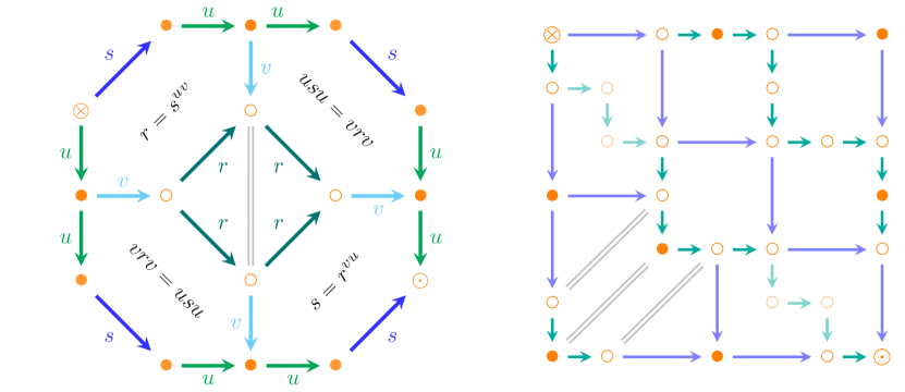
Figure 15. Two ways of decomposing of higher braid relation $\operatorname{Sb}=\operatorname{Br}^{4}$
Left: 2 thin-DB and 2 Sym-Hex; Right: 8 Non-Sym-Hex

Remark 4.5 (Alternative decomposition of $\operatorname{Sb}$ via non-symmetric hexagon relations).

There is another type of (non–symmetric) hexagon relation, appearing in the cluster braid groupoids of type $I_{2}(4)=B_{2}=C_{2}$ Dynkin diagrams, see the picture below.

(4.4)

These relations clearly different from our new thin dumbbell/symmetric hexagon relations. Nevertheless, they both produce $\operatorname{Sb}$ relation in different fashion. See the right picture of Figure 15 that $\operatorname{Sb}$ relation decomposes into 8 non-symmetric hexagons.

In general, there are polygonal (i.e. $(h+2)$-gon) relations (cf. [HHQ]) of the form $x^{2}=y^{h}$, which essentially come from weighted folding for type $I_{2}(h)$ quiver/diagram and produces $\operatorname{Br}^{h}$ relations.

Recall that we have chosen an initial triangulation $\mathbb{T}\in\operatorname{FG}(\mathbf{S}_{\Delta}^{\text{\Sun}})$.

By (3.11), we have a short exact sequence:

$$1\to\pi_{1}\operatorname{FG}^{\mathbb{T}}(\mathbf{S}_{\Delta}^{\text{\Sun}},\mathbb{T})\to\pi_{1}\operatorname{FG}(\mathbf{S}^{\text{\Sun}},\mathrm{T})\xrightarrow{i_{\mathrm{T}}}\operatorname{MT}^{\text{\Sun}}\to 1$$ (4.5)

for $\mathrm{T}=F_{*}^{\Delta}(\mathbb{T})$. By formula (3.9) and (3.10), there is a natural homomorphism

$$\begin{array}[]{rcl}i_{\mathrm{T}}\colon\operatorname{FT}(\mathrm{T})&\twoheadrightarrow&\operatorname{MT}(\mathbb{T})\;\big{(}\lhd\operatorname{MT}(\mathbf{S}_{\Delta}^{\text{\Sun}})\lhd\operatorname{MT}^{\text{\Sun}}\big{)}\\ t_{i}&\mapsto&B_{\eta},\\ l_{j}&\mapsto&L_{\delta},\end{array}$$ (4.6)

for $\eta\in\mathbb{T}^{*}_{\operatorname{CA}}$ dual to a non self-fold arc in $\mathrm{T}$ that corresponds to vertex $i$ in $Q_{\mathrm{T}}$ and, for $\delta\in\mathbb{T}^{*}_{\operatorname{LA}}$ dual to a self-fold arc in $\mathrm{T}$ that corresponds to vertex $j$ in $Q_{\mathrm{T}}$.

5. Properties of flip twist groups

We study relations between flip twist groups associated to different triangulations and their relations with the corresponding mixed twist groups in this section.

5.1. Conjugation formulae

2-cycle twist groups

Let $\mathrm{T}$ be a triangulation of $\mathbf{S}^{\text{\Sun}}$ in $\operatorname{FG}(\mathbf{S}^{\text{\Sun}})$ and $P\in\leftmoon(\mathrm{T})$ a $\mathrm{T}$-isolated puncture, locally shown as $\mathrm{T}_{L}$ in Figure 12. There is a loop twist $s$ associated to the self-folded edge (or vertex $2$ there) and a 2-cycle twist $u^{2}$ associated to the enclosing edge. Call the conjugated twist

$$(u^{2})^{\underline{s}}=su\cdot u\underline{s}\xlongequal{usu=vrv}\underline{u}vrv\cdot u\underline{s}\xlongequal{r=s^{\underline{uv}}}\underline{u}vvu=(v^{2})^{u}$$

the 2-cycle (twist) associated to the loop $s$ at $\mathrm{T}$ of $\operatorname{\mathcal{FG}}(\mathbf{S}^{\text{\Sun}})$. Then to each triangulation of $\operatorname{\mathcal{FG}}(\mathbf{S}^{\text{\Sun}})$, there are $n$ associated 2-cycle twists.

Definition 5.1.

The 2-cycle twist group $\operatorname{CT}(\mathrm{T})$ is the subgroup of $\operatorname{FT}(\mathrm{T})$ generated by all 2-cycle twists at $\mathrm{T}$.

Twist groups related by a flip

We now study the relationship between the flip twist groups of triangulations that differ by a flip. Recall that $\leftmoon(\mathrm{T})$ denotes the set of punctures that are enclosed in some self-folded $\mathrm{T}$-triangles.

Consider a pair of forward flips between two triangulations (which may coincide):

in $\operatorname{\mathcal{FG}}(\mathbf{S}^{\text{\Sun}})$ at arcs $z_{\circ}$ and $z_{\bullet}$ respectively. Denote by $i$ the corresponding vertex in $Q_{\mathrm{T}_{\circ}}$ and $Q_{\mathrm{T}_{\bullet}}$. Note that $\leftmoon(\mathrm{T}_{\circ})$ and $\leftmoon(\mathrm{T}_{\bullet})$ differ by at most one puncture. Without loss of generality, suppose that $\leftmoon(\mathrm{T}_{\circ})\subset\leftmoon(\mathrm{T}_{\bullet})$. The flip twist of $\mathrm{T}_{*}$ with respect to a vertex $i$ of $Q_{\mathrm{T}_{*}}$ will be denoted by $t^{*}_{i}$ or $l^{*}_{i}$.

Lemma 5.2.

[Conjugation formulae]

• If the flip $\mu_{i}$ is a loop in $\operatorname{FG}(\mathbf{S}^{\text{\Sun}})$, i.e. as $\mu_{\circ}=\mu_{2}=s$ at $\mathrm{T}_{\circ}=\mathrm{T}_{L}=\mathrm{T}_{\bullet}$ in Figure 12. Then there is a conjugation/isomorphism

  $$\begin{array}[]{rcl}\operatorname{ad}_{\mu_{\circ}}=\operatorname{ad}_{s}\colon\operatorname{FT}(\mathrm{T}_{\circ})&\to&\operatorname{FT}(\mathrm{T}_{\bullet}),\\ f&\mapsto&f^{s}.\end{array}$$

• If $\leftmoon(\mathrm{T}_{\circ})=\leftmoon(\mathrm{T}_{\bullet})$ and $\mathrm{T}_{\circ}\neq\mathrm{T}_{\bullet}$, then there is a natural isomorphism

  $$\begin{array}[]{rcl}\operatorname{ad}_{\mu_{\circ}}\colon\operatorname{FT}(\mathrm{T}_{\circ})&\xrightarrow{\cong}&\operatorname{FT}(\mathrm{T}_{\bullet}),\\ t^{\circ}_{i}&\mapsto&t^{\bullet}_{i},\\ l^{\circ}_{j}&\mapsto&l^{\bullet}_{j},\\ t^{\circ}_{k}&\mapsto&\underline{t^{\bullet}_{i}}t^{\bullet}_{k}t^{\bullet}_{i},\end{array}$$

  for any $j$ in $Q_{\mathrm{T}_{\circ}}$ corresponding to a self-fold arc for any $k\neq i$ in $Q_{\mathrm{T}_{\circ}}$ corresponding to a non self-fold arc. More precisely, one has $\operatorname{ad}_{\mu_{\circ}}(t^{\circ}_{k})=t^{\bullet}_{k}$ if and only if there is no arrow from $k$ to $i$ in $Q_{\mathrm{T}_{\circ}}$.

• If $\leftmoon(\mathrm{T}_{\bullet})=\leftmoon(\mathrm{T}_{\circ})\cup\{P\}$, i.e. as $(\mathrm{T}_{\circ},\mathrm{T}_{\bullet})=(\mathrm{T}_{M},\mathrm{T}_{L})$ and $\mu_{\circ}=v,\mu_{\bullet}=u$ in Figure 12. Then there is an injection

  $$\begin{array}[]{rcl}\operatorname{ad}_{\mu_{\circ}}=\operatorname{ad}_{v}\colon\operatorname{FT}(\mathrm{T}_{M})&\to&\operatorname{FT}(\mathrm{T}_{L}),\\ t^{M}_{1}&\mapsto&t^{L}_{1},\\ t^{M}_{2}&\mapsto&l^{L}_{2}t^{L}_{1}\underline{l^{L}_{2}},\\ t^{M}_{3}&\mapsto&\underline{t^{L}_{1}}t^{L}_{3}t^{L}_{1},\\ f^{M}_{k}&\mapsto&f^{L}_{k},\end{array}$$ (5.1)

  with vertices $1,2,3$ of $Q_{\mathrm{T}_{M}}$ shown in Figure 12 and any other vertex $k$ with flip twist $f^{?}_{k}$ in $\mathrm{T}_{?}$. In fact, we have $\operatorname{FT}(\mathrm{T}_{L})=\langle\operatorname{FT}(\mathrm{T}_{M})^{\mu},l_{2}^{L}\rangle$ for $l_{2}^{L}=s$.

When restricted to $\operatorname{CT}$, we always have a natural isomorphism

$$\begin{array}[]{rcl}\operatorname{ad}_{\mu_{\circ}}\colon\operatorname{CT}(\mathrm{T}_{\circ})&\to&\operatorname{CT}(\mathrm{T}_{\bullet}),\\ f&\mapsto&f^{s}.\end{array}$$ (5.2)

Proof.

For the first case, the formula for $\operatorname{ad}_{\mu}(t_{z})$ follows from the higher braid relation $\operatorname{Sb}(s,u)$ as we have seen in Figure 15.

For the second case, it follows essentially the same way as [KQ2, Prop. 2.8]. The only difference is that for $j$ corresponding to a self-fold arc, there is no edge between $j$ and $i$ – otherwise $\leftmoon(\mathrm{T}_{\circ})\neq\leftmoon(\mathrm{T}_{\bullet})$. Hence $(l^{\circ}_{j})^{\mu_{i}}=l^{\bullet}_{j}$ is a square-commutation relation.

For the third case, we have

• For $1$, $(t^{M}_{1})^{u}=(u^{2})^{u}=u^{2}=t^{L}_{1}$.

• For $2$, $(t^{M}_{2})^{u}=(v^{2})^{u}=\underline{u}v^{2}u$ and $l^{L}_{2}t^{L}_{1}\underline{l^{L}_{2}}=su^{2}\underline{s}$. Then

  $$usuu\xlongequal{usu=vrv}vrvu\xlongequal{r=s^{\underline{uv}}}vvus$$

  (or the combination of the two hexagon relations on the right in Figure 14) implies that $(t^{M}_{2})^{u}=l^{L}_{2}t^{L}_{1}\underline{l^{L}_{2}}$.

• For $3$, $(t^{M}_{3})^{u}=\underline{t^{L}_{2}}t^{L}_{3}t^{L}_{2}$ follows the same way as in the second case.

• For $k=4$, $(t^{M}_{4})^{u}=t^{L}_{4}$ is a Fat-DB relation.

• For other $k$, $(f^{M}_{k})^{u}=f^{L}_{k}$ is a square=commutation relation (as there is no arrows between $i=2$ and $k$).∎

Note that the flip twist groups are NOT all isomorphic to each other by (5.1).

As a consequence, the 2-cycle twist groups are all isomorphic to each other. In fact, a more precise statement can be made as follows.

Corollary 5.3.

$\{\operatorname{CT}(\mathrm{T})\mid\mathrm{T}\in\operatorname{\mathcal{FG}}(\mathbf{S}^{\text{\Sun}})\}$ is a normal subgroupoid of $\pi_{1}\operatorname{\mathcal{FG}}(\mathbf{S}^{\text{\Sun}})$.

Proof.

This is the analogue of the result of first paragraph [KQ2, Prop. 2.9], which follows the same way since we have the conjugation isomorphisms (5.2). ∎

The $\lozenge$-flips

Definition 5.4.

[FST] A (forward) $\lozenge$-flip is the composition of locally flipping twice at a enclosing edge of a self-folded triangle of a triangulation $\mathrm{T}$ of $\mathbf{S}^{\text{\Sun}}$.

Lemma 5.5.

Consider a pair of $\lozenge$-flips between admissible triangulations as in Figure 12. Then there is a natural isomorphism

$$\begin{array}[]{rcl}\operatorname{ad}_{uv}\colon\operatorname{FT}(\mathrm{T}_{L})&\to&\operatorname{FT}(\mathrm{T}_{R}),\\ t^{L}_{1}&\mapsto&l^{R}_{1}t^{R}_{2}\underline{l^{R}_{1}},\\ l^{L}_{2}&\mapsto&l^{R}_{1},\\ t^{L}_{4}&\mapsto&(t^{R}_{4})^{t^{R}_{2}l^{R}_{1}t^{R}_{2}\underline{l^{R}_{1}}},\\ f^{L}_{k}&\mapsto&f^{R}_{k},\end{array}$$ (5.3)

Proof.

Applying (5.1) twice, we have

$$\begin{array}[]{ccccc}\operatorname{FT}(\mathrm{T}_{L})&\xleftarrow{(-)^{u}}&\operatorname{FT}(\mathrm{T}_{M})&\xrightarrow{(-)^{v}}&\operatorname{FT}(\mathrm{T}_{R}),\\ t^{L}_{1}&\mapsfrom&t^{M}_{1}&\mapsto&l^{R}_{1}t^{R}_{2}\underline{l^{R}_{1}},\\ l^{L}_{2}t^{L}_{1}\underline{l^{L}_{2}}&\mapsfrom&t^{M}_{2}&\mapsto&t^{R}_{2},\\ \underline{t^{L}_{1}}t^{L}_{3}t^{L}_{1}&\mapsfrom&t^{M}_{3}&\mapsto&t^{R}_{3},\\ t^{L}_{4}&\mapsfrom&t^{M}_{4}&\mapsto&\underline{t^{R}_{2}}t^{R}_{4}t^{R}_{2},\\ f^{L}_{k}&\mapsfrom&f^{M}_{k}&\mapsto&f^{R}_{k},\\ \end{array}$$ (5.4)

Thus, we deduce that

$$\begin{cases}(t^{L}_{1})^{uv}=\big{(}(t^{L}_{1})^{\underline{u}}\big{)}^{u^{2}v}=(t^{M}_{1})^{u^{2}v}\xlongequal{u^{2}=t^{M}_{1}}(t^{M}_{1})^{v}=l^{R}_{1}t^{R}_{2}\underline{l^{R}_{1}},\\ (l^{L}_{2})^{uv}=s^{uv}=r=l^{R}_{1},\\ (t^{L}_{3})^{uv}=\Big{(}(t^{L}_{1})^{\underline{u}}\cdot\big{(}\underline{t^{L}_{1}}t^{L}_{3}t^{L}_{1}\big{)}^{\underline{u}}\cdot(\underline{t^{L}_{1}})^{\underline{u}}\Big{)}^{u^{2}v}=(t_{1}^{M}t_{3}^{M}\underline{t_{1}^{M}})^{t^{M}_{1}v}=(t_{3}^{M})^{v}=t_{3}^{R},\\ (t^{L}_{4})^{uv}=\big{(}t_{4}^{M}\big{)}^{u^{2}v}=\big{(}(t_{4}^{M})^{t^{M}_{1}}\big{)}^{v}=\big{(}\underline{t^{R}_{2}}t^{R}_{4}t^{R}_{2}\big{)}^{l^{R}_{1}t^{R}_{2}\underline{l^{R}_{1}}}\\ (f^{L}_{k})^{uv}=\big{(}(f_{k}^{M})^{t^{M}_{1}}\big{)}^{v}\xlongequal{\operatorname{Co}(f_{k}^{M},t^{M}_{1})}(f_{k}^{M})^{v}=f_{k}^{R},\end{cases}$$

as required. ∎

Combining with the fact, [QZ1, Lem. A.2], that any two admissible triangulations in $\operatorname{FG}(\mathbf{S}^{\text{\Sun}})$ are related by a sequence of $\lozenge$-flips. We know that all $\operatorname{FT}(\mathrm{T})$ are isomorphic for admissible triangulations. We proceed to show that flip twist groups at admissible triangulations are the whole point groups/fundamental groups of $\operatorname{\mathcal{FG}}(\mathbf{S}^{\text{\Sun}})$.

5.2. Simply connectedness

Proposition 5.6.

For any admissible triangulation $\mathrm{T}_{0}$, $\operatorname{FT}(\mathrm{T}_{0})=\pi_{1}(\operatorname{\mathcal{FG}}(\mathbf{S}^{\text{\Sun}}),\mathrm{T}_{0})$.

Proof.

We first show that, for any triangulation $\mathrm{T}$, there is a path/morphism

(5.5)

in $\operatorname{\mathcal{FG}}(\mathbf{S}^{\text{\Sun}})$, such that $\leftmoon(\mathrm{T}_{i})\subset\leftmoon(\mathrm{T}_{i+1})$ for any $i$. To do this, we first keep all the self-folded edges in $\mathrm{T}$ (or equivalently cut them), and (repeatedly) flip $\mathrm{T}$ to an admissible triangulation $\mathrm{T}^{\prime}$, such that along the way, $\leftmoon(\mathrm{T}_{i})$ is not decreasing. This can be done due to connectedness of flip graphs of triangulations. Then by [QZ1, Lem. A.2] again, we can $\lozenge$-flip $\mathrm{T}^{\prime}$ to $\mathrm{T}_{0}$ to get a path $p$ as claimed. Note that along the way, we can get rid of any loops in $p$ since they are redundant. By formulae in Lemma 5.2 and Lemma 5.5, the path $p$ induces a conjugation $\operatorname{ad}_{p}\colon\operatorname{FT}(\mathrm{T})\to\operatorname{FT}(\mathrm{T}_{0})$, which is an injection.

Now, take any path/morphism $w$ from $\mathrm{T}$ to $\mathrm{T}_{0}$ in $\operatorname{\mathcal{FG}}(\mathbf{S}^{\text{\Sun}})$. We claim that the conjugation $\operatorname{ad}_{w}$ above is still an injection. By Corollary 5.3, $\operatorname{ad}_{w}$ restricts to an isomorphism $\operatorname{CT}(\mathrm{T})\cong\operatorname{CT}(\mathrm{T}_{0})$. We only need to show that for each loop twist $s\in\operatorname{FT}(\mathrm{T})$, $\operatorname{ad}_{w}(s)$ is in $\operatorname{FT}(\mathrm{T}_{0})$. Use induction on the length of ${w}$ starting with the trivial case with $|{w}|=0$. If there is a loop $r$ in the path $w$, i.e. $w=w_{1}rw_{2}$, then $\operatorname{ad}_{w_{2}}(r)$ is in $\operatorname{FT}(\mathrm{T}_{0})$ by induction. As

$$\operatorname{ad}_{w}(s)=\underline{w_{2}rw_{1}}sw_{1}rw_{2}=\underline{r}^{w_{2}}s^{w_{1}w_{2}}r^{w_{2}}=\underline{\operatorname{ad}_{w_{2}}(r)}\cdot\operatorname{ad}_{w_{1}w_{2}}(s)\cdot\operatorname{ad}_{w_{2}}(r),$$

we only need to show that $\operatorname{ad}_{w_{1}w_{2}}(s)$ is in $\operatorname{FT}(\mathrm{T}_{0})$. In other words, we can get rid of all loop twists in ${w}$. Since $\operatorname{ad}_{w}(s)=(\underline{w}p)\cdot\operatorname{ad}_{p}(s)\cdot(\underline{p}w)$, we only need to show that $\underline{p}w$ is in $\operatorname{FT}(\mathrm{T}_{0})$. Note that $\underline{p}w$ does not contain any loop twist. By Theorem 3.1, when regarding $\underline{p}w$ as a path in $\underline{\operatorname{EG}}(\mathbf{S}^{\text{\Sun}})$, it decomposes into (unoriented) squares and pentagons. Taking account of the orientation, this means that $\underline{p}w$ in $\operatorname{FG}(\mathbf{S}^{\text{\Sun}})$ can be written a product of oriented squares/pentagons, together with 2-cycles. On the other hand, all the 2-cycles are in the 2-cycle twist subgroupoid by Corollary 5.3. Thus, $\underline{p}w$ is in $\operatorname{CT}(\mathrm{T}_{0})\leq\operatorname{FT}(\mathrm{T}_{0})$ as required.

So we have shown that the conjugations of any 2-cycles and loops $\operatorname{\mathcal{FG}}(\mathbf{S}^{\text{\Sun}})$ by any paths are in $\operatorname{FT}(\mathrm{T}_{0})$. On the other hand, let $\underline{\operatorname{\mathcal{EG}}}(\mathbf{S}^{\text{\Sun}})$ be the groupoid obtained from $\underline{\operatorname{EG}}(\mathbf{S}^{\text{\Sun}})$ by composing square/pentagon relations. Consider the canonical functor $\operatorname{\mathcal{FG}}(\mathbf{S}^{\text{\Sun}})\to\underline{\operatorname{\mathcal{EG}}}(\mathbf{S}^{\text{\Sun}})$, which sets all 2-cycles and loops equal to 1. By Theorem 3.1, $\pi_{1}\underline{\operatorname{\mathcal{EG}}}(\mathbf{S}^{\text{\Sun}})$ is trivial and hence $\operatorname{\mathcal{FG}}(\mathbf{S}^{\text{\Sun}})$ is generated by 2-cycles and loops. This implies that $\operatorname{FT}(\mathrm{T}_{0})=\pi_{1}(\operatorname{\mathcal{FG}}(\mathbf{S}^{\text{\Sun}}),\mathrm{T}_{0})$. ∎

An immediate consequence is the following.

Corollary 5.7.

• $\operatorname{MT}^{\text{\Sun}}=\operatorname{MT}(\mathbf{S}_{\Delta}^{\text{\Sun}})$.

• $\overline{\operatorname{FG}_{\text{\tiny{$\copyright$}}}^{\circ}[\mathbb{T}_{0},\mathbb{T}_{0}[1]]}^{\circlearrowleft}=\operatorname{FG}(\mathbf{S}^{\text{\Sun}})$ if $\mathbb{T}$ is admissible.

Proof.

Choose admissible triangulations $\mathbb{T}$ and $\mathrm{T}$, (4.6) implies that $\operatorname{MT}(\mathbb{T})=\operatorname{MT}^{\text{\Sun}}$, which implies the first claim. Combining with (3.12), the second claim follows. ∎

Now we can prove the main theorem of this section.

Theorem 5.8.

$\operatorname{\mathcal{FG}}^{\mathbb{T}}(\mathbf{S}_{\Delta}^{\text{\Sun}})$ is a universal cover of $\operatorname{\mathcal{FG}}(\mathbf{S}^{\text{\Sun}})$ with covering group $\operatorname{MT}(\mathbf{S}_{\Delta}^{\text{\Sun}})$ and $i_{\mathrm{T}}$ in (4.6) restricts to a natural isomorphism $\operatorname{FT}(\mathrm{T})\cong\operatorname{MT}(\mathbb{T})$, which further restricts to an isomorphism $\operatorname{CT}(\mathrm{T})\cong\operatorname{BT}(\mathbf{S}_{\Delta}^{\text{\Sun}})$ .

Proof.

In the case when $\mathrm{T}$ (and $\mathbb{T}$) is admissible, $i_{\mathrm{T}}$ in (4.6) becomes $\operatorname{FT}(\mathrm{T})\twoheadrightarrow\operatorname{MT}(\mathbb{T})$, sending the standard generators to the standard ones. On the other hand, by Corollary 2.13, there is a presentation of $\operatorname{MT}(\mathbb{T})$, with three type of relations (e.g. $\operatorname{Co},\operatorname{Br}$ and $\operatorname{Sb}$). Each of which, also holds for (the standard generators of) $\operatorname{FT}(\mathrm{T})$, as shown in Lemma 4.4. Thus, $i_{\mathrm{T}}$ admits a well-defined inverse that forces it to be an isomorphism.

In the case when $\mathrm{T}$ (and $\mathbb{T}$) is not admissible, the isomorphism $i_{\mathrm{T}}$ restricts to an isomorphism (4.6) between subgroups of $\pi_{1}\operatorname{FG}(\mathbf{S}^{\text{\Sun}},\mathrm{T})\cong\operatorname{MT}(\mathbf{S}_{\Delta}^{\text{\Sun}})$. ∎

Another related consequence is that we obtain Corollary 3.6 therefore.

6. On fundamental groups of moduli spaces

6.1. Quadratic differentials

Let $\mathbf{X}$ be a compact Riemann surface and $\omega_{\mathbf{X}}$ be its holomorphic cotangent bundle. A meromorphic quadratic differential $\phi$ on $\mathbf{X}$ is a meromorphic section of the line bundle $\omega_{\mathbf{X}}^{2}$. In terms of a local coordinate at $z$ on $\mathbf{X}$, $\phi$ can be written as $\phi(z)=g(z)\,dz^{2}$, for a meromorphic function

$$g(z)=z^{d}(a_{d}+a_{d+1}z+\cdots)$$

for $a_{d}\neq 0$. If $d>0$, $z$ is a zero of order $d$; if $d<0$, $z$ is a pole of order $-d$; if $d=0$, $z$ is a smooth point. The zeros and poles are singularities/critical points of $\phi$. For $d\in\mathbb{Z}_{>0}$, denote by $\mathbf{w}_{d}(\phi)$ the set of zeroes of order $d$ and $\mathbf{w}_{-d}(\phi)$ the set of poles of order $d$. There are two type of singularities:

• the finite type, including all zeroes and simple (i.e. order 1) poles. Let

  $$\mathbf{w}_{\operatorname{fin}}=(\mathbf{w}_{-1},\mathbf{w}_{0},\mathbf{w}_{1},\cdots)$$

  be the collection of them.

• the infinite type, including all poles with order at least two. Let

  $$\mathbf{w}_{\operatorname{inf}}=(\mathbf{w}_{-2},\mathbf{w}_{-3},\cdots)$$

  be the collection of them.

Denote by $\mathbf{X}^{\circ}=\mathbf{X}^{\circ}(\phi)=\mathbf{X}\smallsetminus(\mathbf{w}_{\operatorname{fin}}\cup\mathbf{w}_{\operatorname{inf}})$.

In general, one could also allow a set $\mathbf{w}_{0}(\phi)$ of special smooth markings of $\phi$ in $\mathbf{X}$.

Foliation structure

The key structure of quadratic differentials is the foliation structure. At a smooth point of $\mathbf{X}^{\circ}$, there is a distinguished local coordinate $\omega=\int\sqrt{g(z)}dz$, uniquely defined up to transformations: $\omega\mapsto\pm\,\omega+\operatorname{const}$, with respect to which, one has $\phi(\omega)=d\omega\otimes d\omega$. Then by locally pulling back the Euclidean metric on $\mathbb{C}$ using a distinguished coordinate $\omega$, $\phi$ induces the $\phi$-metric and geodesics on $\mathbf{X}$. Each geodesics have a constant phase with respect to $\omega$.

A trajectory of a $\phi$ on $\mathbf{X}$ is a maximal geodesic $\gamma\colon(0,1)\to\mathbf{X}^{\circ}$, with respect to the $\phi$ metric (i.e. corresponds to the equation $\operatorname{Im}\omega\equiv\operatorname{const}$). When $\lim\gamma(t)$ exists in $\mathbf{X}$ as $t\to 0$ (resp. $t\to 1$), the limits are called the left (resp. right) endpoint of $\gamma$. The horizontal trajectories (with $\operatorname{Im}\omega\equiv 0$) of a meromeorphic quadratic differential $\phi$ provide the horizontal foliation on $\mathbf{X}$.

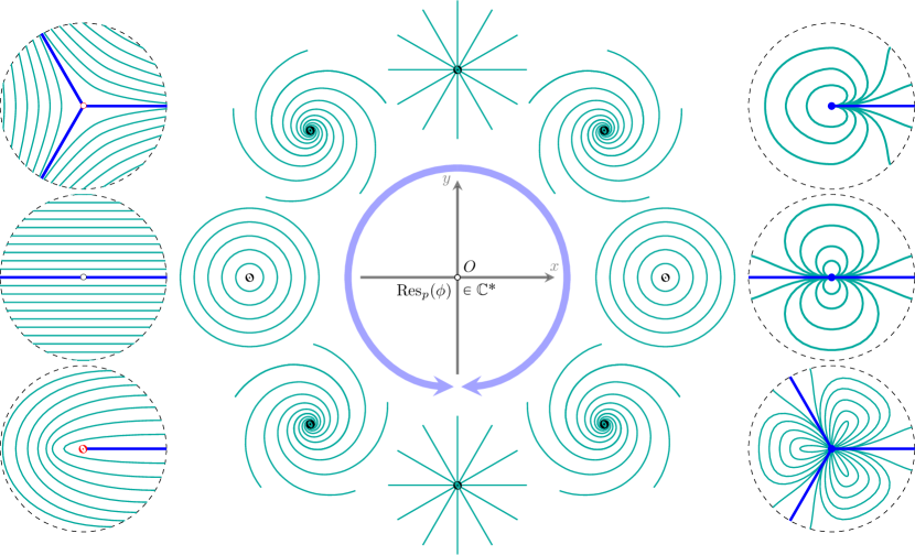
Figure 16. Foliation structure around a point of a Riemann surface

In Figure 16, one has examples of (horizontal) foliations. Namely:

• On the left column, the pictures show the foliation at a simple zero/smooth point/simple pole (up to bottom). In general, there are $d+2$ distinguished directions at a finite singularity (conical point) of order $d\geq-1$ that divides the neighbourhood of such a point into $d+2$ (local) half planes at zero.

• In the middle column, the pictures show the foliation at a double pole $p$ depending on the residue

  $$\operatorname{Res}_{p}(\phi)\colon=\pm 2\int_{\widetilde{\delta_{p}}}\sqrt{\phi},$$ (6.1)

  of $\phi$ at $p$, where the integration is along the lift $\widetilde{\delta_{p}}$ of a small loop $\delta_{p}$ on the spectral cover (w.r.t. $\phi$) of $\mathbf{X}$.

• On the right column, the pictures show the foliation at a pole of order 3/4/5 (up to bottom). In general, there are $|d|-2$ distinguished directions at a pole of order $d\leq-3$ that divides the neighbourhood of such a point into $d+2$ (local) half planes at infinity.

Horizonal strip decomposition

There are the following types of trajectories of a quadratic differential:

• saddle trajectories, either whose both ends are in $\mathbf{w}_{\operatorname{fin}}$.

• separating trajectories with one endpoint in $\mathbf{w}_{\operatorname{fin}}$ and the other in $\mathbf{w}_{\operatorname{inf}}$;

• generic trajectories whose both ends are in $\mathbf{w}_{\operatorname{fin}}$;

• recurrent if at least one of its directions is recurrent.

But from now on, we now fix the horizonal direction to unless specified otherwise, i.e. trajectories means horizontal trajectories. A saddle connection is a trajectory in some arbitrary direction and a saddle trajectory means a horizontal saddle connection.

Removing from $\mathbf{X}$ the separating trajectories and saddle trajectories, it decomposes the surface into connected components, each of which is of the following types:

• a horizontal strip, i.e. is isomorphic to $\{z\in\mathbb{C}\mid a<\operatorname{Im}(z)<b\}$ equipped with the differential $dz^{2}$ for some $a<b\in\mathbb{R}$. It is swept out by generic trajectories connecting two (not necessarily distinct) poles.

• a half-plane, i.e. is isomorphic to $\{z\in\mathbb{C}\mid\operatorname{Im}(z)>0\}$ equipped with the differential $dz^{2}$. It is swept out by generic trajectories which connect a fixed pole to itself.

• a ring domain or cylinder, i.e. is foliated by closed trajectories.

• a spiral domain, i.e. is the interior of the closure of a recurrent trajectory.

We call this union the horizontal strip decomposition of $\mathbf{X}$ with respect to $\phi$.

A quadratic differential $\phi$ on $\mathbf{X}$ is saddle-free, if it has no saddle trajectory. Then there are only half-planes and horizontal strips by [BS, Lem. 3.1]. Note that in such a case:

• In each horizontal strip, the trajectories are isotopic to each other.

• The boundary of any component consists of separating trajectories.

• In each horizontal strip, there is a unique geodesic, the saddle connection, connecting the two zeroes on its boundary.

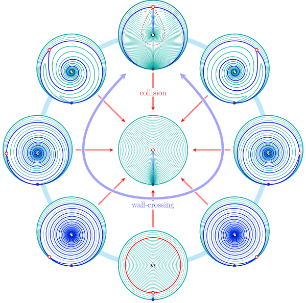
Figure 17. A loop in $\operatorname{FQuad}(\mathbf{S}^{\text{\Sun}})$ with a missing center in $\operatorname{FQuad}(\mathbf{S}^{\text{\YinYang}})$

Example 6.1.

Figure 17 shows several local horizontal strip decompositions on $\mathbf{X}$ corresponding to the motion of a L-flip at a self-folded triangle (the top picture). In particular, there is a ‘wall crossing’ state (the bottom picture) when there is a saddle trajectory (red cycle), which bounds a degenerate ring domain (meaning one of its boundary components is a double pole). Note that, in the pictures

• the emerald/blue vertices (bullets) are poles or marked points,

• the black/red suns are double/simple poles respectively,

• the red vertices (small circles) are simple zeroes,

• the emerald arcs are (generic) geodesics,

• the blue arcs are separating trajectories,

• the red solid arc/cycle is a saddle trajectory (in the bottom picture) and the red dashed arc is a saddle connection (in the top picture).

Moreover, Figure 17 demonstrates a loop in the moduli space of quadratic differentials which corresponds to the L-twist (as the bottom picture of Figure 2) of the saddle connection in the top picture.

For comparison, see the left picture of Figure 1 (or [KQ2, Fig. 4.3]) for the horizontal strip decompositions pictures of another loop in the moduli space, which corresponds to a braid twist (as the top picture of Figure 2).

The real blow-up of $\mathbf{X}$ with respect to $\phi$ is a weighted DMSp $\mathbf{X}^{\phi}_{\mathbf{w}_{\operatorname{fin}}}$ obtained from $\mathbf{X}$ by replacing each puncture $p$ in $\mathbf{w}_{\leq-3}$ with a boundary component $\partial_{p}$ with $\operatorname{ord}_{\phi}(p)-2$ marked points and regarding $\mathbf{w}_{\operatorname{fin}}=\Delta$ as decoration set with weights given by the degree of the finite singularities, $\mathbf{w}_{-2}=\text{\Sun}$ as puncture set. One can also forget about the decorations and denote by $\mathbf{X}^{\phi}$ the corresponding weighted marked surface with punctures.

Moduli spaces and framing

The moduli space $\operatorname{Quad}(g)$ of quadratic differentials on genus $g$ Riemann surfaces decomposes into many strata, parameterized by their prescribed singularity type, i.e.

$$\operatorname{Quad}(g)=\bigsqcup_{|\mathbf{w}|=4g-4}\operatorname{Quad}(g;\mathbf{w}_{\operatorname{fin}},\mathbf{w}_{\operatorname{inf}}),$$

where

$$\|\mathbf{w}\|=\|\mathbf{w}_{\operatorname{fin}}\|+\|\mathbf{w}_{\operatorname{inf}}\|\colon=\sum_{k\in\mathbb{Z}}k|\mathbf{w}_{k}|$$ (6.2)

satisfying $\|\mathbf{w}\|=4g-4$, for $|\mathbf{w}_{k}|$ the number of points in $\mathbf{w}_{k}$.

The numerical data of singularity type of $\phi$ on $\mathbf{X}$ is $(\mathbf{w}_{\operatorname{fin}},\mathbf{w}_{\operatorname{inf}})$, which can be encoded by the associated weighted DMSp $\mathbf{X}^{\phi}_{\mathbf{w}_{\operatorname{fin}}}$. We will only consider the strum $\operatorname{Quad}(g;\mathbf{w}_{1},\mathbf{w}_{\operatorname{inf}})$ for $\mathbf{w}_{\operatorname{fin}}=\mathbf{w}_{1}$ (i.e. only simple zeros as finite singularities) in this section and $\mathbf{w}_{\operatorname{inf}}\neq\mathbf{w}_{-2}$ (i.e. not only just double poles as infinite singularities). In such a case, a quadratic differential in $\operatorname{Quad}(g;\mathbf{w}_{1},\mathbf{w}_{\operatorname{inf}})$ is parameterized by a DMSp $\mathbf{S}_{\Delta}^{\text{\Sun}}$ (with trivial weight).

More precisely, a point $(\mathbf{X},\phi,\psi)$ in

$$\operatorname{Quad}(\mathbf{S}^{\text{\Sun}})=\operatorname{Quad}(\mathbf{S}_{\Delta}^{\text{\Sun}})=\operatorname{Quad}(g;\mathbf{w}_{1},\mathbf{w}_{\operatorname{inf}})$$

consists of a Riemann surface $\mathbf{X}$ with quadratic differential $\phi$, equipped with a diffeomorphism $\psi\colon\mathbf{S}^{\text{\Sun}}\to\mathbf{X}^{\phi}$, preserving the marked points and punctures. Two such quadratic differentials $(\mathbf{X}_{1},\phi_{1},\psi_{1})$ and $(\mathbf{X}_{2},\phi_{2},\psi_{2})$ are equivalent, if there exists a biholomorphism $f\colon\mathbf{X}_{1}\to\mathbf{X}_{2}$ such that $f^{*}(\phi_{2})=\phi_{1}$ and furthermore $\psi_{2}^{-1}\circ f_{*}\circ\psi_{1}\in\operatorname{Diff}(\mathbf{S}^{\text{\Sun}})$, where $f_{*}\colon\mathbf{X}_{1}^{\phi_{1}}\to\mathbf{X}_{2}^{\phi_{2}}$ is the induced diffeomorphism.

As discussed in [KQ2, § 4.1], there are two natural way to frame on $\operatorname{Quad}(\mathbf{S}^{\text{\Sun}})$. Namely, in the definition above, if we change $\operatorname{Diff}(\mathbf{S}^{\text{\Sun}})$ to $\operatorname{Diff}_{0}(\mathbf{S}^{\text{\Sun}})$ to identify equivalent elements, then we obtain the $\mathbf{S}^{\text{\Sun}}$-framed moduli space $\operatorname{FQuad}(\mathbf{S}^{\text{\Sun}})$. Similarly, we can also use $\mathbf{S}_{\Delta}^{\text{\Sun}}$ to frame, i.e. replacing the diffeomorphism $\psi\colon\mathbf{S}^{\text{\Sun}}\to\mathbf{X}^{\phi}$ by a diffeomorphism $\psi\colon\mathbf{S}_{\Delta}^{\text{\Sun}}\to\mathbf{X}^{\phi}_{\mathbf{w}_{1}}$ preserving the marked points, punctures and decorations. These three moduli spaces fits in the following diagram:

(6.3)

For a $\mathbf{S}_{\Delta}^{\text{\Sun}}$-framed the generic trajectories on $\mathbf{X}$ (with respect to $\phi$) are inherited by $\mathbf{S}$, for any $\psi\colon\mathbf{S}\to\mathbf{X}^{\phi}$, and all trajectories on $\mathbf{X}$ (with respect to $\phi$) are inherited by $\mathbf{S}_{\Delta}$, for any $\Psi\colon\mathbf{S}_{\Delta}\to\mathbf{X}^{\phi}$.

So generic trajectories become open arcs on $\mathbf{S}$ (as well as on $\mathbf{S}_{\Delta}$) and saddle trajectories/connections becomes closed arcs on $\mathbf{S}_{\Delta}$.

Example 6.2.

The foliations in Figure 17 are precisely a loop in the once-punctured monogon case, i.e. $\operatorname{Quad}(\mathbf{S}^{\text{\Sun}})=\operatorname{Quad}(0;1,-2,-3)$. One can write down the quadratic differentials globally (on $\mathbb{C}\mathbb{P}^{1}$):

$$\operatorname{Quad}(0;1,-2,-3)=\{c\in\mathbb{C}^{*}\mid\phi(z)=\frac{z+c}{z^{2}}dz^{2}\}.$$

More precisely

• The residue at the double pole (i.e. zero) is $s=\operatorname{Res}_{0}(\phi)=4\pi\mathbf{i}\sqrt{c}$.

• The central foliation in Figure 17 correspond to the $c=0$ case: then the quadratic differential $\phi(z)=z^{-1}dz^{2}$ is in $\operatorname{Quad}(0;-1,-3)$.

Moreover, in this case, we have

• $\operatorname{FQuad}(\mathbf{S}^{\text{\Sun}})=\operatorname{Quad}(\mathbf{S}^{\text{\Sun}})\cong\mathbb{C}^{*}$.

• $\operatorname{FQuad}(\mathbf{S}_{\Delta}^{\text{\Sun}})=\{\operatorname{log}(c)\mid c\in\mathbb{C}^{*}\}\cong\mathbb{C}$ is the $\mathbb{Z}$-cover/universal cover of $\operatorname{FQuad}(\mathbf{S}^{\text{\Sun}})$.

6.2. Cell structures

Stratification

Let $\Psi\operatorname{FQuad}(\mathbf{S}_{\Delta}^{\text{\Sun}})$. One has the following numerical equality:

$$r_{\Psi}+2s_{\Psi}+t_{\Psi}=\|\mathbf{w}_{\operatorname{fin}}\|+2|\mathbf{w}_{\operatorname{fin}}|=\sum_{k=-1}^{\infty}(\mathbf{w}_{k}+2)=\colon K$$

where $s_{\Psi}/r_{\Psi}/t_{\Psi}$ are the numbers of saddle/recurrent/separating trajectories, respectively.

There is a natural filtration of $\operatorname{FQuad}(\mathbf{S}_{\Delta}^{\text{\Sun}})$ given by

$$B_{0}=B_{1}\subset B_{2}\subset\cdots\subset B_{K}=\operatorname{Quad}(\mathbf{S}_{\Delta}^{\text{\Sun}}),$$

for

$$B_{p}=B_{p}(\mathbf{S}_{\Delta}^{\text{\Sun}})=\{\Psi\in\operatorname{Quad}(\mathbf{S}_{\Delta}^{\text{\Sun}}):r_{\Psi}+2s_{\Psi}\leq p\},$$ (6.4)

observing that $B_{0}=B_{1}$ is the set of saddle-free differentials. The corresponding stratification is given by $F_{p}(\mathbf{S}_{\Delta}^{\text{\Sun}})=B_{p}\smallsetminus B_{p-1}$.

The space $B_{2}$ is called the space of tame differentials, We observe that $F_{0}$ is dense, $F_{1}$ is empty, and $F_{2}$ consists of differentials with exactly one saddle trajectory. Here are two more precisely statements.

Lemma 6.3.

[BMQS, Lem. 4.1] $\operatorname{FQuad}(\mathbf{S}_{\Delta}^{\text{\Sun}})=\mathbb{C}\cdot B_{0}(\mathbf{S}_{\Delta}^{\text{\Sun}})$ and hence $B_{0}(\mathbf{S}_{\Delta}^{\text{\Sun}})$ is dense in $\operatorname{FQuad}(\mathbf{S}_{\Delta}^{\text{\Sun}})$. Moreover, $F_{2}(\mathbf{S}_{\Delta}^{\text{\Sun}})$ has codimension 1 and $B_{2}(\mathbf{S}_{\Delta}^{\text{\Sun}})$ has codimension 2.

Lemma 6.4.

[BMQS, Cor. 4.3] The connected components of $\operatorname{FQuad}(\mathbf{S}_{\Delta}^{\text{\Sun}})$ naturally correspond to the connected components of $\operatorname{FG}(\mathbf{S}_{\Delta}^{\text{\Sun}})$.

All the statements above also apply to the $\mathbf{S}^{\text{\Sun}}$-framed version.

WKB-triangulations

Let

$$\mathbf{H}_{\circ}=\{z\in\mathbb{C}\mid\operatorname{Im}(z)>0\}\subset\mathbb{C}$$

be the strict upper half plane and $\mathbf{H}=\mathbf{H}_{\circ}\cup\mathbb{R}_{<0}$ the half-open-half-closed one.

Let $\Psi$ be a saddle-free $\mathbf{S}_{\Delta}^{\text{\Sun}}$-framed quadratic differential. Then there is an associated (WKB-)triangulation $\mathbb{T}_{\Psi}$ of $\mathbf{S}_{\Delta}^{\text{\Sun}}$, where the arcs are (isotopy classes of inherited) generic trajectories. The dual graph $\mathbb{T}_{\Psi}^{*}$ consisting of saddle connections. Denote by $\operatorname{U}^{\circ}(\mathrm{T})$ be the subspace in $\operatorname{FQuad}(\mathbf{S}^{\text{\Sun}})$ consisting of those saddle-free $\Psi$ support on $\mathrm{T}$ (i.e. whose associated triangulation is $\mathrm{T}$). Then $\operatorname{U}(\mathrm{T})\cong\mathbf{H}^{\mathrm{T}}$ and

$$B_{0}(\mathbf{S}^{\text{\Sun}})=\bigcup_{\mathrm{T}\in\operatorname{FG}(\mathbf{S}^{\text{\Sun}})}\operatorname{U}^{\circ}(\mathrm{T}).$$ (6.5)

for $\operatorname{U}^{\circ}(\mathrm{T})\cong\mathbf{H}_{\circ}^{\mathrm{T}}$. The coordinates $(u_{\gamma})_{\gamma\in T}$ give the complex modulus of the horizontal strip with generic trajectory in the isotopy class $\gamma$. Thus the $\operatorname{U}^{\circ}(\mathrm{T})$ are precisely the connected components of $B_{0}(\mathbf{S})$. The boundary of $\operatorname{U}^{\circ}(\mathrm{T})$ meets $F_{2}(\mathbf{S})$ in $2n$ connected components, which we denote $\partial^{\sharp}_{\gamma}\operatorname{U}^{\circ}(\mathrm{T})$ and $\partial^{\flat}_{\gamma}\operatorname{U}^{\circ}(\mathrm{T})$, where the coordinate $u_{\gamma}$ goes to the negative or positive real axis, respectively. Note that $u_{\gamma}$ cannot go to zero since it means the collision of two zeros.

By Walls-have-Ends property ([BS, Prop 5.8] for simple zero case and [BMQS, Cor. 4.3] in general), we have the following, showing that $\operatorname{FG}(\mathbf{S}_{\Delta}^{\text{\Sun}})$ is a skeleton for $\operatorname{FQuad}^{\mathbb{T}}(\mathbf{S}_{\Delta}^{\text{\Sun}})$.

Lemma 6.5.

There is a (unique up to homotopy) canonical embedding

$$\wp_{\mathbf{S}_{\Delta}^{\text{\Sun}}}\colon\operatorname{FG}^{\mathbb{T}}(\mathbf{S}_{\Delta}^{\text{\Sun}})\to\operatorname{FQuad}^{\mathbb{T}}(\mathbf{S}_{\Delta}^{\text{\Sun}})$$ (6.6)

whose image is dual to $B_{2}(\mathbf{S}_{\Delta}^{\text{\Sun}})$ and which induces a surjective map

(6.7)

Again, these statements also apply to the $\mathbf{S}^{\text{\Sun}}$-framed version. For the later use, we record them as well: there is a canonical embedding

$$\wp_{\mathbf{S}^{\text{\Sun}}}\colon\operatorname{FG}(\mathbf{S}^{\text{\Sun}})\to\operatorname{FQuad}(\mathbf{S}^{\text{\Sun}})$$ (6.8)

that induces a surjective map

(6.9)

Parallel to the cell structure of moduli spaces of quadratic differentials, one has stability structures on triangulated categories, see Section A.2. We recall a upgraded version of Theorem 3.7.

Theorem 6.6.

[CHQ, Thm. 1.1] The isomorphism (3.4) can be complexified to an isomorphism between complex manifolds

$$\begin{array}[]{rcl}\operatorname{X}^{\text{\Sun}}_{*}\colon\operatorname{FQuad}^{\mathbb{T}}(\mathbf{S}_{\Delta}^{\text{\Sun}})&\cong&\operatorname{Stab}^{\mathbb{T}}(\operatorname{\mathcal{D}}_{3}(\mathbf{S}_{\Delta}^{\text{\Sun}})),\\ s\cdot\Psi&\mapsto&s\cdot(Z,\operatorname{\mathcal{H}}_{\mathbb{T}_{\Psi}}),\end{array}$$ (6.12)

for any $s\in\mathbb{C}$ and saddle free $\mathbf{S}_{\Delta}^{\text{\Sun}}$-framed quadratic differential $\Phi$, where

$$Z(X_{\eta})=\int_{\widetilde{\eta}}\sqrt{\Psi}.$$ (6.13)

In Appendix B, we will study a quotient version of (6.12):

$$\operatorname{Quad}(\mathbf{S}^{\text{\Sun}})=\operatorname{FQuad}(\mathbf{S}^{\text{\Sun}})/\operatorname{MCG}(\mathbf{S}^{\text{\Sun}})\cong\operatorname{Stab}^{\mathbb{T}}(\operatorname{\mathcal{D}}_{3}(\mathbf{S}_{\Delta}^{\text{\Sun}}))\operatorname{Aut}^{\circ},$$ (6.14)

where $\operatorname{Aut}^{\circ}$ is a quotient group of the autoequivalence group of $\operatorname{\mathcal{D}}_{3}(\mathbf{S}_{\Delta}^{\text{\Sun}})$, cf. (B.7).

6.3. The kernel of AJ map as the fundamental group

Proposition 6.7.

Square, Pentagon, Hexagon and dumbbell relations holds in $\operatorname{Stab}^{\circ}$.

Proof.

Namely, the square, pentagon and the Fat-DB follows precisely as in the proof of [KQ2, Prop.4.14]. The other two new relations (Thin-DB and Sym-Hex) follows in a similar fashion. We sketch the proof as follows.

By Theorem 3.7, Thin-DB or Sym-Hex in $\operatorname{FG}^{\mathbb{T}}(\mathbf{S}_{\Delta}^{\text{\Sun}})$ induces the corresponding hexagons in $\operatorname{EG}^{\mathbb{T}}(\operatorname{\mathcal{D}}_{3}(\mathbf{S}_{\Delta}^{\text{\Sun}}))$ as shown in Figure 18 and Figure 19.

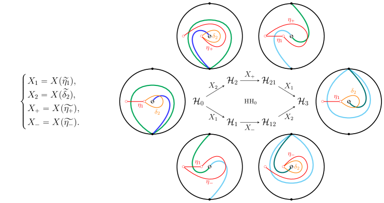
Figure 18. Thin-DB in $\operatorname{EG}^{\mathbb{T}}(\operatorname{\mathcal{D}}_{3}(\mathbf{S}_{\Delta}^{\text{\Sun}}))$

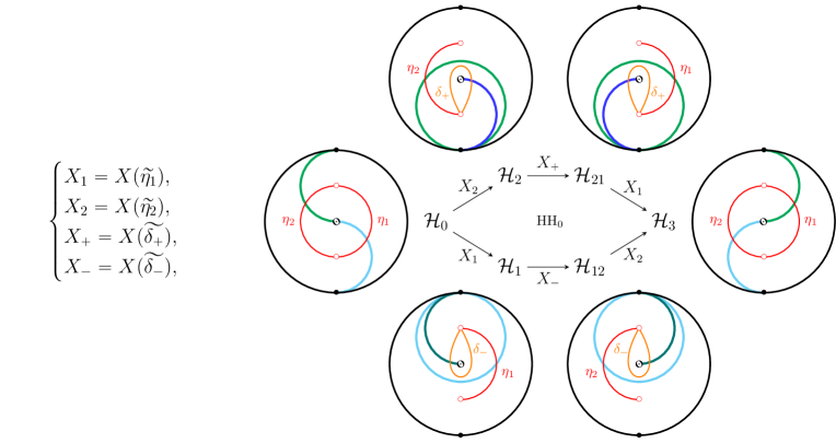
Figure 19. Sym-Hex in $\operatorname{EG}^{\mathbb{T}}(\operatorname{\mathcal{D}}_{3}(\mathbf{S}_{\Delta}^{\text{\Sun}}))$

In fact, such induced hexagons can be described in the same way in $\operatorname{EG}^{\mathbb{T}}(\operatorname{\mathcal{D}}_{3}(\mathbf{S}_{\Delta}^{\text{\Sun}}))$ by setting the simples $X_{1},X_{2}$ in the source heart $\operatorname{\mathcal{H}}_{0}$ correspond to the proper (graded) closed arcs as the formulae shown in the left of the figures. Then there are always two short exact sequences in $\operatorname{\mathcal{H}}_{0}$

$$0\to X_{2}\to X_{+}\to X_{1}\to 0,$$ (6.15)

$$0\to X_{1}\to X_{-}\to X_{+}\to 0.$$ (6.16)

and the same hexagon of hearts (=$\operatorname{HH}_{0}$) in $\operatorname{FG}^{\mathbb{T}}(\operatorname{\mathcal{D}}_{3}(\mathbf{S}_{\Delta}^{\text{\Sun}}))$ with

$$\begin{cases}\operatorname{\mathcal{H}}_{i}=(\operatorname{\mathcal{H}}_{0})_{X_{i}}^{\sharp},\;i=1,2\\ \operatorname{\mathcal{H}}_{21}=(\operatorname{\mathcal{H}}_{2})_{X_{+}}^{\sharp},\\ \operatorname{\mathcal{H}}_{12}=(\operatorname{\mathcal{H}}_{1})_{X_{-}}^{\sharp},\\ \operatorname{\mathcal{H}}_{3}=(\operatorname{\mathcal{H}}_{21})_{X_{1}}^{\sharp}=(\operatorname{\mathcal{H}}_{12})_{X_{2}}^{\sharp},\end{cases}$$

which consists of two paths:

$$\begin{cases}\operatorname{HH}_{0}^{+}\colon\operatorname{\mathcal{H}}_{0}\to\operatorname{\mathcal{H}}_{2}\to\operatorname{\mathcal{H}}_{21}\to\operatorname{\mathcal{H}}_{3},\\ \operatorname{HH}_{0}^{-}\colon\operatorname{\mathcal{H}}_{0}\to\operatorname{\mathcal{H}}_{1}\to\operatorname{\mathcal{H}}_{12}\to\operatorname{\mathcal{H}}_{3}.\end{cases}$$

Note that the rigidities of the simple tiltings are different in these two cases.

Now we use the $\mathbb{C}$-action to show that such induced hexagons are contractible. Namely, we can choose $\sigma_{\pm}$ in $\operatorname{U}(\operatorname{\mathcal{H}}_{0})$ such that

$$\begin{cases}Z_{+}(X_{1}[1])=\exp 3\pi\mathbf{i}\delta,&\\ Z_{+}(X_{2}[1])=\exp\pi\mathbf{i}\delta,&\end{cases}\quad\begin{cases}Z_{-}(X_{1}[1])=\exp\pi\mathbf{i}\delta,&\\ Z_{-}(X_{2}[1])=\exp 3\pi\mathbf{i}\delta,&\end{cases}$$ (6.17)

$$Z_{\pm}(X)=M\cdot\exp\textstyle{\frac{\mathbf{i}\pi}{2}},\qquad X\in\operatorname{Sim}\operatorname{\mathcal{H}}_{0}\smallsetminus\{X_{1},X_{2}\}$$ (6.18)

for some real number $M\gg 1$. for some small $\delta\in\mathbb{R}_{>0}$ and large $M\in\mathbb{R}_{>0}$ as shown in Figure 20.

Figure 20. Central charges of $\sigma_{+},\sigma_{-}$

Then we can deduce from (6.15) that $X_{\pm}$ is stale with respect to $\sigma_{\pm}$ but unstable with respect to $\sigma_{\mp}$. Furthermore, by the simple tilting formulae in [CHQ, App. A], we deduce that $k\delta\cdot\sigma_{+}$, for $k=1,2,3$, are in the three tilting walls of the path $\operatorname{HH}_{0}^{+}$ while $(k\delta-\delta,k\delta)\cdot\sigma_{+}$ is in the corresponding cube $\operatorname{U}^{\circ}(\operatorname{\mathcal{H}}_{l})$ for $k/l=1/0,2/2,3/21,4/3$. Hence we deduce that $[0,4\delta]\cdot\sigma_{+}$ is homotopy to $\wp_{*}(\operatorname{HH}_{0}^{+})$. Similarly, we have $[0,4\delta]\cdot\sigma_{-}$ is homotopy to $\wp_{*}(\operatorname{HH}_{0}^{-})$. Then if we connect $\sigma_{\pm}$ with a line segment $l$ in $\operatorname{U}^{\circ}(\operatorname{\mathcal{H}}_{0})$, we see that $4\delta\cdot l$ will be in $\operatorname{U}^{\circ}(\operatorname{\mathcal{H}}_{3})$ and the boundary of the rectangle $[0,4\delta]\cdot l$ is homotopy to $\wp_{*}(\operatorname{HH}_{0})$. Thus, $\wp_{*}(\operatorname{HH}_{0})$ is contractible as required. ∎

By Equation 6.6 and Proposition 6.7, the simply connectedness of $\operatorname{\mathcal{FG}}^{\mathbb{T}}(\mathbf{S}_{\Delta}^{\text{\Sun}})$ implies the simply connectedness of $\operatorname{Stab}^{\mathbb{T}}(\operatorname{\mathcal{D}}_{3}(\mathbf{S}_{\Delta}^{\text{\Sun}}))$.

Theorem 6.8.

$\operatorname{Stab}^{\mathbb{T}}(\operatorname{\mathcal{D}}_{3}(\mathbf{S}_{\Delta}^{\text{\Sun}}))$ is simply connected and hence is a universal cover of $\operatorname{FQuad}(\mathbf{S}^{\text{\Sun}})$.

Combining Theorem 2.6 (that $\operatorname{MT}(\mathbf{S}_{\Delta}^{\text{\Sun}})=\ker\operatorname{AJ}$) and the characterization of connected components (in Corollary 3.6 and Lemma 6.4), we obtain our main theorem.

Theorem 6.9.

Let $\mathbf{S}_{\Delta}^{\text{\Sun}}$ be a DMSp. There is a short exact sequence

$$1\to\pi_{1}\operatorname{FQuad}(\mathbf{S}^{\text{\Sun}})\to\operatorname{SBr}(\mathbf{S}_{\Delta}^{\text{\Sun}})\xrightarrow{\operatorname{AJ}}\operatorname{\bf H}_{1}(\mathbf{S})\to 1$$ (6.19)

Moreover, we have

$$\begin{cases}\pi_{1}\operatorname{FQuad}^{\mathbb{T}}(\mathbf{S}_{\Delta}^{\text{\Sun}})=1,\\ \pi_{0}\operatorname{FQuad}(\mathbf{S}_{\Delta}^{\text{\Sun}})\cong\operatorname{\bf H}_{1}(\mathbf{S}).\end{cases}$$ (6.20)

6.4. Corollaries

Extending the Abel-Jacobi map to $\operatorname{MCG}(\mathbf{S}_{\Delta}^{\text{\Sun}})$

The following is a version of Octahedron Axiom in the group setting.

Lemma 6.10.

Let $P\lhd G$ be a normal subgroup of $G$ and $f\colon G\to G_{0}$ a group homomorphism such that $f\mid_{P}$ is surjective. Denote by $S=\ker(f)$ and $M=\ker(f\circ i)$, where $i$ is the inclusion $P\to G$. Then we have

• $M=P\cap S$ and $G=P\cdot S$.

• $G/P\cong S/M$ and $G/M=(G/P)\times(P/M)$.

So there is the following commutative diagram:

(6.21)

Proof.

It is straightforward see $M=P\cap S$. Then by the Diamond (=$2^{nd}$ Isomorphism) Theorem, we have $P\cdot S/S\cong P/M=G_{0}=G/S$. Thus, $G=P\cdot S$. Using the Diamond Theorem again, we have $G/P\cong S/M$. Finally, quotienting by $M$, we have $G/M=(P/M)\cdot(S/M)$. But $(P/M)\cap(S/M)=(P\cap S)/M=1$, which implies that $G/M=(P/M)\times(S/M)$. ∎

Taking $S=\operatorname{SBr}(\mathbf{S}_{\Delta}^{\text{\Sun}})\lhd\operatorname{MCG}(\mathbf{S}_{\Delta}^{\text{\Sun}})=G$, $G_{0}=\operatorname{MCG}(\mathbf{S}^{\text{\Sun}})$ and $f=F^{\Delta}_{*}$. Then $M=\operatorname{MT}(\mathbf{S}_{\Delta}^{\text{\Sun}})$, $P=\pi_{1}\operatorname{Quad}(\mathbf{S}^{\text{\Sun}})$ and (6.21) becomes (6.22) in the introduction.

Corollary 6.11.

We have

$$\operatorname{MCG}(\mathbf{S}_{\Delta}^{\text{\Sun}})/\pi_{1}\operatorname{Quad}(\mathbf{S}^{\text{\Sun}})\cong\operatorname{\bf H}_{1}(\mathbf{S})$$

$$\operatorname{MCG}(\mathbf{S}_{\Delta}^{\text{\Sun}})/\operatorname{MT}(\mathbf{S}_{\Delta}^{\text{\Sun}})=\operatorname{\bf H}_{1}(\mathbf{S}^{\text{\Sun}})\times\operatorname{MCG}(\mathbf{S})$$

that fit into the commutative diagram (6.22).

(6.22)

Appendix A Tilting and stability structures

A.1. Simple tilting theory

We will first recall basic notions and notations about triangulated categories, tilting theory and the 3-Calabi-Yau categories associated to a DMSp. Then we review the categorification of flip graphs from [CHQ], cf. [Qy2, Chr].

We work over algebraically closed field $\mathbf{k}$ and $\mathbf{k}$-linear additive categories. A category usually means an abelian or triangulated category. Most stuffs in this subsection are classical, we refer to [Bri, KQ1, Qy1] for general references.

We write $\mathcal{C}=\mathcal{T}\perp\mathcal{F}$ for a torsion pair in a category $\mathcal{C}$. An object $S$ in $\mathcal{C}$ is rigid if $\operatorname{Ext}^{1}(S,S)=0$.

For an abelian category $\operatorname{\mathcal{H}}$, denote by $\operatorname{Sim}\operatorname{\mathcal{H}}$ the set of simples of $\operatorname{\mathcal{H}}$. Such an $\operatorname{\mathcal{H}}$ is called finite if $\operatorname{Sim}\operatorname{\mathcal{H}}$ is finite and generates $\operatorname{\mathcal{H}}$ (so that $\operatorname{\mathcal{H}}$ is a length category).

Let $\operatorname{\mathcal{D}}$ be a triangulated category. A t-structure $\mathcal{P}$ of $\operatorname{\mathcal{D}}$ is the torsion part of a torsion pair $\operatorname{\mathcal{D}}=\mathcal{P}\perp\mathcal{P}^{\perp}$ such that $\mathcal{P}[1]\subset\mathcal{P}$. It is bounded if

$$\mathcal{D}=\displaystyle\bigcup_{i,j\in\mathbb{Z}}\mathcal{P}^{\perp}[i]\cap\mathcal{P}[j],$$

The heart of a bounded t-structure $\mathcal{P}$ is $\operatorname{\mathcal{H}}=\mathcal{P}^{\perp}[1]\cap\mathcal{P}$, which is abelian and determines $\mathcal{P}$ uniquely. For any object $E\in\operatorname{\mathcal{D}}$, there is a HN-filtration

(A.1)

with factors $F_{i}\in\operatorname{\mathcal{H}}[k_{i}]$ for $k_{1}>k_{2}>\cdots>k_{l}$.

Given a torsion pair $\operatorname{\mathcal{H}}=\mathcal{T}\perp\mathcal{F}$ in $\operatorname{\mathcal{H}}$, there is a new heart $\operatorname{\mathcal{H}}^{\sharp}$, known as the forward (HRS) tilt of $\operatorname{\mathcal{H}}$ with respect to the torsion pair (cf. [HRS]), which admits a torsion pair $\mathcal{F}[1]\perp\mathcal{T}$ (and hence determined by them). The dual notion of forward tilting is backward tilting. For $\operatorname{\mathcal{H}}=\mathcal{T}\perp\mathcal{F}$, one has $\operatorname{\mathcal{H}}^{\flat}=\operatorname{\mathcal{H}}^{\sharp}[-1]=\mathcal{F}\perp\mathcal{T}[-1]$.

There is a natural partial order on the set of hearts, i.e.

$$\operatorname{\mathcal{H}}_{1}\leq\operatorname{\mathcal{H}}_{2}\;\Longleftrightarrow\;\mathcal{P}_{2}\subset\mathcal{P}_{1}\;\Longleftrightarrow\;\mathcal{P}^{\perp}_{1}\subset\mathcal{P}^{\perp}_{2}.$$ (A.2)

Another way to characterize forward tilts of a heart is that they are precisely all heart in the interval $[\operatorname{\mathcal{H}},\operatorname{\mathcal{H}}[1]]$, i.e. (cf. [KQ1, § 3])

$$\operatorname{\mathcal{H}}^{\prime}=\operatorname{\mathcal{H}}^{\sharp}\text{ w.r.t. $\operatorname{\mathcal{H}}=\mathcal{T}\perp\mathcal{F}$ if and only if}\operatorname{\mathcal{H}}\leq\operatorname{\mathcal{H}}^{\prime}\leq\operatorname{\mathcal{H}}[1].$$ (A.3)

Indeed, in such a case, one has $\mathcal{T}=\operatorname{\mathcal{H}}^{\prime}\cap\operatorname{\mathcal{H}}$ and $\mathcal{F}=\operatorname{\mathcal{H}}^{\prime}[-1]\cap\operatorname{\mathcal{H}}$.

Definition A.1.

[KQ1] A forward tilting $\operatorname{\mathcal{H}}\to\operatorname{\mathcal{H}}^{\sharp}$ with respect to $\operatorname{\mathcal{H}}=\mathcal{T}\perp\mathcal{F}$ is simple if the corresponding torsion part $\mathcal{F}$ is generated by a single simple $S\in\operatorname{Sim}\operatorname{\mathcal{H}}$. Denote by $\operatorname{\mathcal{H}}^{\sharp}_{S}$ the simple forward tilt in this case and by $\mu_{S}^{\sharp}\colon S\to\operatorname{\mathcal{H}}^{\sharp}_{S}$ the simple forward tilting.

A backward tilting is simple if the corresponding torsion part is generated by a single simple $S$ and the backward tilt will be denoted by $\operatorname{\mathcal{H}}^{\flat}_{S}$. The backward tilting is the inverse operation of forward tilting and we have $\mu_{S[-1]}^{\sharp}\colon\operatorname{\mathcal{H}}^{\flat}_{S}\to\operatorname{\mathcal{H}}$.

The exchange graph (of hearts) $\operatorname{EG}(\operatorname{\mathcal{D}})$ of a triangulated category $\operatorname{\mathcal{D}}$ is the directed graph whose vertices are hearts and whose edges are simple forward tilting. When $\operatorname{\mathcal{D}}$ admits a canonical heart $\operatorname{\mathcal{H}}$, denote by $\operatorname{EG}^{\circ}(\operatorname{\mathcal{D}})$ the principal component of $\operatorname{EG}(\operatorname{\mathcal{D}})$, i.e. the connected component containing $\operatorname{\mathcal{H}}$.

We often interested in intervals of in $\operatorname{EG}^{\circ}(\operatorname{\mathcal{D}})$. Denote by $\operatorname{EG}^{\circ}[\operatorname{\mathcal{H}}_{1},\operatorname{\mathcal{H}}_{2}]$ the connected component of the full subgraph $\operatorname{EG}^{\circ}(\operatorname{\mathcal{D}})\cap[\operatorname{\mathcal{H}}_{1},\operatorname{\mathcal{H}}_{2}]$ containing $\operatorname{\mathcal{H}}_{1}$.

There are couple of simple tilting formulae, e.g [KQ1, Prop. 5.4] for the rigid case and [CHQ] for a slight generalization.

In many good scenarios, $\operatorname{EG}^{\circ}(\operatorname{\mathcal{D}})$ will consists of finite hearts and the formula apply to any of its edges. In that case, $\operatorname{EG}^{\circ}(\operatorname{\mathcal{D}})$ is $(n,n)$-regular, e.g. when $\operatorname{\mathcal{D}}=\operatorname{\mathcal{D}}^{b}(Q)$ for an acyclic quiver $Q$ or $\operatorname{\mathcal{D}}=\operatorname{\mathcal{D}}_{N}(Q)$ for the $N$-Calabi-Yau version of $\operatorname{\mathcal{D}}^{b}(Q)$.

As rigid simple tilting is very nice and we introduce the rigid exchange graph $\operatorname{EG}_{\circledR}(\operatorname{\mathcal{D}})$ to be the subgraph of $\operatorname{EG}(\operatorname{\mathcal{D}})$ whose edge are simple tilting with respect to rigid simples. Similar for other variation of $\operatorname{EG}$, e.g. $\operatorname{EG}^{\circ}$, $\operatorname{EG}^{\circ}[\operatorname{\mathcal{H}}_{1},\operatorname{\mathcal{H}}_{2}]$, etc. Note that the formula above only ensures the finiteness of the tilted heart, not the rigidity of the tilted simples. Hence, $\operatorname{EG}_{\circledR}^{\circ}(\operatorname{\mathcal{D}})$ may not be equal $\operatorname{EG}^{\circ}(\operatorname{\mathcal{D}})$ even if it is $(n,n)$-regular.

We recall another technical result from [KQ1, Lem. 3.8].

Lemma A.2.

Let $\operatorname{\mathcal{H}}\in\operatorname{EG}^{\circ}[\operatorname{\mathcal{H}}_{0},\operatorname{\mathcal{H}}_{0}[1]]$. Then, for any rigid $S\in\operatorname{Sim}\operatorname{\mathcal{H}}$, it must be in one of $\operatorname{\mathcal{H}}_{0}$ or $\operatorname{\mathcal{H}}_{0}[1]$ and

• ${\operatorname{\mathcal{H}}}^{\sharp}_{S}\in\operatorname{EG}^{\circ}[\operatorname{\mathcal{H}}_{0},\operatorname{\mathcal{H}}_{0}[1]]$ if and only if $S\in\operatorname{\mathcal{H}}_{0}$ if and only if $S\notin\operatorname{\mathcal{H}}_{0}[1]$.

• ${\operatorname{\mathcal{H}}}^{\flat}_{S}\in\operatorname{EG}^{\circ}[\operatorname{\mathcal{H}}_{0},\operatorname{\mathcal{H}}_{0}[1]]$ if and only if $S\notin\operatorname{\mathcal{H}}_{0}$ if and only if $S\in\operatorname{\mathcal{H}}_{0}[1]$.

In other words, exactly one of ${\operatorname{\mathcal{H}}}^{\pm\sharp}_{S}$ is still in $\operatorname{EG}^{\circ}[\operatorname{\mathcal{H}}_{0},\operatorname{\mathcal{H}}_{0}[1]]$.

A.2. Stability structures on triangulated categories

Let $\operatorname{\mathcal{D}}$ be a triangulated category. Recall the basic notion and result from [Bri].

Definition A.3.

[Bri, Def.] A stability condition $\sigma=(Z,\mathcal{P})$ consists of a central charge $Z\in\operatorname{Hom}(\operatorname{K}(\operatorname{\mathcal{D}}),\mathbb{C})$ and a $\mathbb{R}$-family $\mathcal{P}_{\mathbb{R}}=\{\mathcal{P}(\phi)\mid\phi\in\mathbb{R}\}$ of additive (in fact, abelian) subcategories (known as the slicing), satisfying (cf. [Bri] for more details):

• if $0\neq E\in\mathcal{P}(\phi)$, then $Z(E)=m(E)\exp(\phi\pi\mathbf{i})$ for some $m(E)\in\mathbb{R}_{>0}$;

• $\mathcal{P}(\phi+1)=\mathcal{P}(\phi)[1]$, for all $\phi\in\mathbb{R}$;

• $\operatorname{Hom}(\mathcal{P}(\phi_{1}),\mathcal{P}(\phi_{2}))=0$ if $\mathcal{P}(\phi_{1})>\mathcal{P}(\phi_{2})$;

• each nonzero object $E\in\mathcal{D}$ admits a Harder-Narashimhan filtration (A.1) with factors $F_{i}\in\mathcal{P}(\phi_{i})$ for $\phi_{1}>\cdots>\phi_{l}$. The upper and lower phases of $E$ are $\phi_{1}$ and $\phi_{l}$ respectively.

• the so-called support property.

Objects in the slice $\mathcal{P}(\phi)$ are called semistable objects with phase $\phi$; simple objects in $\mathcal{P}(\phi)$ is called stable objects with phase $\phi$. For an interval $J$, denote by $\mathcal{P}(J)$ the subcategory consisting of objects whose upper and lower phases are in $J$. The heart $\operatorname{\mathcal{H}}_{\sigma}$ of a stability condition $\sigma=(Z,\mathcal{P})$ is the abelian category $\mathcal{P}(0,1]$.

Theorem A.4.

[Bri, Thm. 1] All stability conditions on a triangulated category $\operatorname{\mathcal{D}}$ form a complex manifold, denoted by $\operatorname{Stab}(\operatorname{\mathcal{D}})$, with local coordinate given by the central charge.

There are two natural actions on $\operatorname{Stab}(\operatorname{\mathcal{D}})$, the $\mathbb{C}$-action given by

$$s\cdot(Z,\mathcal{P})=(Z\cdot e^{-\mathbf{i}\pi s},\mathcal{P}_{\operatorname{Re}(s)}),$$

for $\mathcal{P}_{x}(\phi)=\mathcal{P}(\phi+x)$ and the $\operatorname{Aut}\operatorname{\mathcal{D}}$-action given by

$$\Phi(Z,\mathcal{P})=\big{(}Z\circ\Phi^{-1},\Phi(\mathcal{P})\big{)}.$$

Generic-finite component

For a finite heart $\operatorname{\mathcal{H}}$, the stability conditions supported in $\operatorname{\mathcal{H}}$ (i.e. with $\operatorname{\mathcal{H}}_{\sigma}=\operatorname{\mathcal{H}}$) is parameterized by the central charges $Z(S)\in\mathbf{H}$ for $S\in\operatorname{Sim}\operatorname{\mathcal{H}}$. Thus there is a cell/subspace $\operatorname{U}(\operatorname{\mathcal{H}})\cong\mathbf{H}^{\operatorname{Sim}\operatorname{\mathcal{H}}}$ in $\operatorname{Stab}(\operatorname{\mathcal{D}})$ consisting of those stability conditions supported on $\operatorname{\mathcal{H}}$.

For each tilting $\operatorname{\mathcal{H}}\to\operatorname{\mathcal{H}}^{\prime}={\operatorname{\mathcal{H}}}^{\sharp}_{S}$, there is co-dimensional one wall where $Z(S)\in\mathbb{R}_{>0}$,

$$\partial^{\sharp}_{S}\operatorname{U}(\operatorname{\mathcal{H}})=\partial^{\flat}_{S[1]}\operatorname{U}(\operatorname{\mathcal{H}}^{\prime})=\overline{\operatorname{U}(\operatorname{\mathcal{H}})}\cap\overline{\operatorname{U}(\operatorname{\mathcal{H}}^{\prime})}.$$

For a connected component $\operatorname{EG}^{\circ}$ in $\operatorname{EG}(\operatorname{\mathcal{D}})$, define

$$B_{0}(\operatorname{EG}^{\circ})=\bigcup_{\operatorname{\mathcal{H}}\in\operatorname{EG}^{\circ}}\operatorname{U}^{\circ}(\operatorname{\mathcal{H}})$$

and

$$B_{2}(\operatorname{EG}^{\circ})=B_{0}(\Gamma)\cup\bigcup_{\begin{smallmatrix}\operatorname{\mathcal{H}}\in\operatorname{EG}^{\circ}\\ S\in\operatorname{Sim}\operatorname{\mathcal{H}}\end{smallmatrix}}\partial^{\sharp}_{S}\operatorname{U}(\operatorname{\mathcal{H}}).$$

A connected component $\operatorname{Stab}^{\circ}$ in $\operatorname{Stab}(\operatorname{\mathcal{D}})$ is generic-finite if $\operatorname{Stab}^{\circ}=\mathbb{C}\cdot B_{2}(\operatorname{EG}^{\circ})$ for some connected component $\operatorname{EG}^{\circ}$ of $\operatorname{EG}(\operatorname{\mathcal{D}})$ consisting of finite hearts.

Appendix B Marked surfaces with mixed punctures & vortices

Recall that there is a partition $\text{\Sun}=\leftmoon\cup{\rightmoon}$. We add extra $\mathbb{Z}/_{2}$-symmetry to punctures in ${\rightmoon}$, call them vortices and use ☯ to denote the set of vortices. Let $\mathbf{S}^{\leftmoon,\text{\YinYang}}$ be the marked surface with mixed punctures & vortices (MSx). More precisely, what this means is:

• Categorically, we will add terms around each vortex in ☯ for quivers with potential associated to triangulations and deform $\operatorname{\mathcal{D}}_{3}(\mathbf{S}_{\Delta}^{\text{\Sun}})$ into $\operatorname{\mathcal{D}}_{3}(\mathbf{S}^{\leftmoon,\text{\YinYang}})$.

• Geometrically, we will allow collisions between simple zeros in $\Delta$ and double poles in ☯, so that we partial compactify the moduli space $\operatorname{FQuad}(\mathbf{S}^{\text{\Sun}})$ into $\operatorname{FQuad}(\mathbf{S}^{\leftmoon,\text{\YinYang}})$ by adding strata with simple poles from collision (with orbifolding).

Then we show that the corresponding quotient space $\operatorname{Stab}\operatorname{\mathcal{D}}_{3}(\mathbf{S}^{\leftmoon,\text{\YinYang}})/\operatorname{Aut}^{\circ}$ is isomorphic to the unframed version of $\operatorname{FQuad}(\mathbf{S}^{\leftmoon,\text{\YinYang}})$. When $\operatorname{\mathcal{D}}_{3}(\mathbf{S}^{\leftmoon,\text{\YinYang}})$ is fully deformed, i.e. taking $\text{\YinYang}=\text{\Sun}$, We will call the corresponding MSx by MSv (with notation $\mathbf{S}^{\text{\YinYang}}$). In such a case, $\operatorname{Quad}(\mathbf{S}^{\text{\YinYang}})$ becomes the moduli space in [BS].

Remark B.1.

We assume the following when considering MSx:

• $\partial\mathbf{S}^{\leftmoon,\text{\YinYang}}\neq\varnothing$.

• $n\geq 2$, where $n$ is defined in (2.19).

The main results are covered in [KQ2] when $\text{\Sun}=\varnothing$ and hence we usually assume $\text{\Sun}\neq\varnothing$ in the proofs.

B.1. Cluster-ish combinatorics for MSx

Signed triangulations of MSx

A signed triangulation $\mathrm{T}^{\times}$ of a MSx $\mathbf{S}^{\leftmoon,\text{\YinYang}}$ consists of an (ideal) triangulation $\mathrm{T}$ of MSp $\mathbf{S}^{\text{\Sun}}$ with a sign

$$\epsilon\colon\text{\YinYang}\to\{\pm 1\}\cong\mathbb{Z}/_{2}.$$ (B.1)

The set of signs can be identified with $\mathbb{Z}/_{2}{}^{{\oplus\text{\YinYang}}}$. Two signed triangulations $\mathrm{T}^{\times}_{1}=(\mathrm{T}_{1},\epsilon_{1})$ and $\mathrm{T}^{\times}_{2}=(\mathrm{T}_{2},\epsilon_{2})$ are equivalent if

• $\mathrm{T}_{1}=\mathrm{T}_{2}$ and

• $\epsilon_{1}(V)=\epsilon_{2}(V)$, for any vortex $V$ that is nott in a self-folded triangle.

Namely, we have the (local) equivalence shown in Figure 21. In other words, the sign at a vortex which is in a self-folded triangulation can be chosen to be arbitrary without changing the equivalent class of signed triangulation.

Figure 21. Equivalent signed triangulations (local)

There is a forward flip between signed triangulations $\mu^{\sharp}\colon\mathrm{T}^{\times}_{1}\to\mathrm{T}^{\times}_{2}$ if one can choose the (representatives of) signs $\epsilon_{1}=\epsilon_{2}$, such that there is a usual forward flip between the corresponding triangulations $\mu^{\sharp}\colon\mathrm{T}_{1}\to\mathrm{T}_{2}$ or there is a forward L-flip between the corresponding triangulations, where the corresponding isolated puncture is not a vortex. For more details, cf. [FST]. Then we have the corresponding notation of (oriented) cluster-ish exchange graph $\operatorname{EG}(\mathbf{S}^{\leftmoon,\text{\YinYang}})$ for MSx.

Alternatively/concretely, $\operatorname{EG}(\mathbf{S}^{\leftmoon,\text{\YinYang}})$ can be constructed as follows. Note that when we write ${\rightmoon}$ instead of ☯, we mean there is no $\mathbb{Z}/_{2}$-symmetry (i.e. signs) attached.

• Denote by $\operatorname{FG}(\mathbf{S}^{\leftmoon,{\rightmoon}})$ the flip graph for $\mathbf{S}^{\leftmoon,{\rightmoon}}$, which is a subgraph of $\operatorname{FG}(\mathbf{S}^{\text{\Sun}})$, by deleting L-flips where the corresponding enclosed puncture is in fact a vortex.

• For each sign $\epsilon\in\mathbb{Z}/_{2}{}^{{\oplus\text{\YinYang}}}$, take a copy $\operatorname{FG}^{\epsilon}(\mathbf{S}^{\leftmoon,{\rightmoon}})=\operatorname{FG}(\mathbf{S}^{\leftmoon,{\rightmoon}})\times\{\epsilon\}$.

• We take the union of $\operatorname{FG}^{\epsilon}(\mathbf{S}^{\leftmoon,{\rightmoon}})$, for all $\epsilon\in\mathbb{Z}/_{2}{}^{{\oplus\text{\YinYang}}}$, and identify vertices/edges by the equivalent relation $\sim$ above.

So we have

$$\operatorname{FG}(\mathbf{S}^{\leftmoon,\text{\YinYang}})=\bigcup_{\epsilon\in\mathbb{Z}/_{2}{}^{{\oplus\text{\YinYang}}}}\operatorname{FG}^{\epsilon}(\mathbf{S}^{\leftmoon,{\rightmoon}})=\big{(}\operatorname{FG}(\mathbf{S}^{\leftmoon,{\rightmoon}})\times\mathbb{Z}/_{2}{}^{{\oplus\text{\YinYang}}}\big{)}\big{/}\sim.$$ (B.2)

There is also an unoriented version of $\operatorname{FG}(\mathbf{S}^{\leftmoon,\text{\YinYang}})$, which can be obtained from it by deleting all loop edges and replacing each 2-cycle with an unoriented edge. Equivalently, one has

$$\underline{\operatorname{EG}}(\mathbf{S}^{\leftmoon,\text{\YinYang}})=\bigcup_{\epsilon\in\mathbb{Z}/_{2}{}^{{\oplus\text{\YinYang}}}}\underline{\operatorname{EG}}^{\epsilon}(\mathbf{S}^{\text{\Sun}})=\big{(}\underline{\operatorname{EG}}(\mathbf{S}^{\text{\Sun}})\times\mathbb{Z}/_{2}{}^{{\oplus\text{\YinYang}}}\big{)}\big{/}\sim.$$ (B.3)

For instance, the left picture of Figure 10 shows the building process of $\operatorname{FG}(\mathbf{S}^{\text{\YinYang}})$ for a once-puncture triangle with $\text{\YinYang}=\text{\Sun}$. When $\text{\YinYang}=\text{\Sun}$, we have $\operatorname{FG}(\mathbf{S}^{\text{\YinYang}})=\operatorname{CEG}(\mathbf{S}^{\text{\Sun}})$ and $\underline{\operatorname{EG}}(\mathbf{S}^{\text{\YinYang}})=\underline{\operatorname{CEG}}(\mathbf{S}^{\text{\Sun}})$ are the oriented and unoriented cluster exchange graph associated to $\mathbf{S}^{\text{\Sun}}$ respectively.

Building on Theorem 3.1, we have the following result as a variation of Theorem 3.1, using the same proof of [FST, Thm.10.2].

Proposition B.2.

$\pi_{1}\underline{\operatorname{EG}}(\mathbf{S}^{\leftmoon,\text{\YinYang}})$ is generated by squares and pentagons, which locally look like the (unoriented) squares/pentagons in Figure 11, or the one in Figure 22.

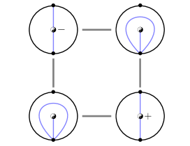
Figure 22. The square involving vortex

Mutation, reduction and right-equivalence

There are the notions of right-equivalence, reduction and mutation introduced by [DWZ], cf. [KY, § 2.1] for more details.

• Two quivers with potential are right-equivalent if there is an algebra isomorphism between the corresponding completed path algebras such that it is the identity when restricted to the vertices and induces cyclically equivalence between the potentials.

• The reduction is an operation on right-equivalent classes of quivers with potential. It reduces a quiver with potential by killing some 2-cycles (and change the potential according). A quiver with potential $(Q,W)$ is called reduced if $\partial_{a}W$ is contained in $\mathfrak{m}^{2}$ for any $a\in Q_{1}$. By [DWZ, Thm. 4.6], the reduction is well-defined on the right-equivalence classes of quivers with potential.

• The mutation $\mu_{i}$ is an operation on a quiver with potential $(Q,W)$ at a vertex $i$ of $Q$; it produces another quiver with potential. By [DWZ, Thm. 5.2 and Thm. 5.7], the mutation is also well-defined up to right-equivalence, which is an involution.

Quivers with potential associated to triangulated MSx

Let $\mathrm{T}^{\times}=(\mathrm{T},\epsilon)$ be a signed triangulation. Define a quiver with potential $(\widehat{Q_{\mathrm{T}^{\times}}^{{\leftmoon,\text{\YinYang}}}},\widehat{W_{\mathrm{T}^{\times}}^{{\leftmoon,\text{\YinYang}}}})$ as follows:

• The vertices are open arcs in $\mathrm{T}$.

• For each triangle $T$ of $\mathrm{T}$, which is not a self-folded triangle enclosing a vortex, there is a (clockwise) 3-cycle between the edges of $T$ (so that the arrow corresponds to (anticlockwise) angles in $T$.

• For each vortex $V$ that is enclosed in a self-folded triangle $T$ with self-folded edge $i$ and loop edge $l$, we call these two edges twins. Add an arrow between $i$ and (from/to) $j$ whenever there is an arrow between $l$ and (from/to) $j$, for $j\neq l$ in $\mathrm{T}$. So besides the usual (type P-1) puzzle piece (i.e. a triangle without involving a vortex in a self-folded triangle–see any triangle in Figure 6), there are three types of other puzzle pieces in a triangulation $\mathrm{T}$ shown in Figure 23.

  

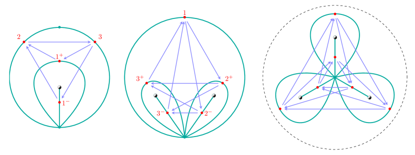
  Figure 23. The quivers with potential associated to types P-2/P-3/P-4 puzzle pieces with vortices

• The unreduced potential is

  $$\widehat{W_{\mathrm{T}^{\times}}^{{\leftmoon,\text{\YinYang}}}}=\sum_{T}W_{T}^{\text{\YinYang}}-\sum_{V}W_{V}^{\text{\YinYang}},$$

  where

  • the first sum is over triangles which is not a self-folded triangle enclosing a vortex, each team $W_{T}^{\text{\YinYang}}$ is the sum of all corresponding 3-cycles (one can replacing an edge of $\mathrm{T}$ with its twin). This means in type P-$k$, there are $2^{k-1}$ 3-cycle terms in $W_{T}^{\text{\YinYang}}$ for the non self-folded triangle $T$.

  • the second sum is over all vortices which are not enclosed in a self-folded triangle $T$, each term $W_{V}^{\text{\YinYang}}$ is an anticlockwise cycle around $V$, which needs to skip some of the arrows. More precisely, if there are twins incident at $V$, which corresponding to another vortex $V_{0}$, then

    • $W_{V}^{\text{\YinYang}}$ skip the self-folded edge at $V_{0}$ and only count loop-edge once if $\epsilon(V_{0})=1$;

    • $W_{V}^{\text{\YinYang}}$ skip the loop-edge and only count self-folded edge if $\epsilon(V_{0})=-1$.

Definition B.3.

Let $(Q_{\mathrm{T}^{\times}}^{{\leftmoon,\text{\YinYang}}},W_{\mathrm{T}^{\times}}^{{\leftmoon,\text{\YinYang}}})$ be the quiver with potential associated to a signed triangulation $\mathrm{T}^{\times}=(\mathrm{T},\epsilon)$ of $\mathbf{S}^{\leftmoon,\text{\YinYang}}$, which is the reduced part of $(\widehat{Q_{\mathrm{T}^{\times}}^{{\leftmoon,\text{\YinYang}}}},\widehat{W_{\mathrm{T}^{\times}}^{{\leftmoon,\text{\YinYang}}}})$.

Example B.4.

For instance, the term $W_{V}^{\text{\YinYang}}$ in the potential is

• a 5-cycle for the left picture of Figure 24;

• a 10-cycle $7\to 8\to 4\to 1\to 2\to 2\to 1\to 3\to 5\to 6\to 7$ for the middle picture of Figure 24;

• a 7-cycle $7\to 8\to 3\to 1^{\epsilon(V)}\to 2\to 5\to 6\to 7$ for the right picture of Figure 24, where $\epsilon(V)$ is the sign of the vortex $V_{0}$ (in a self-folded triangle) adjacent to $V$.

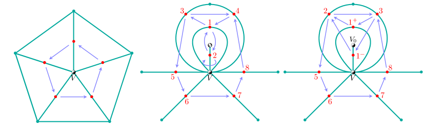
Figure 24. The extra terms in the potential for each vortex (not in a self-folded triangle)

Figure 25 shows a reduction of quiver with potential, where one needs to kill a 2-cycles (around a vortex). For more examples, see [L-F].

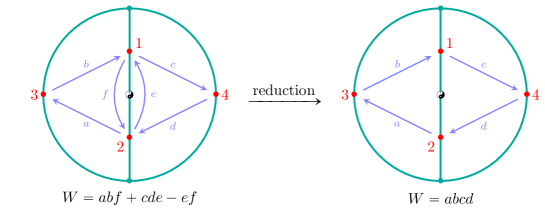
Figure 25. Reduction of a quiver with potential

Note that:

• the quiver with potential is the one we considered in Definition 2.8 if $\text{\YinYang}=\varnothing$;

• the quiver with potential is non-degenerate if and only if $\text{\YinYang}=\text{\Sun}$; in which case, it is the one constructed in [L-F] for classical cluster theory.

Lemma B.5.

Any usual flip of signed triangulations induces mutations between the associated quivers with potential (up to right-equivalence).

Proof.

This is a local issue. We only need to check the following.

• For the usual mutation corresponding to flipping diagonals of a quadrilateral, we know that the corresponding quivers with 3-cycles potential are related by mutation up to right equivalent as below.

  (B.4)

• For the flip $\mu_{1}$ in Figure 6, we cut the self-folded edge (corresponding to vertex 2 in the two pictures in the middle) and the mutation becomes the case above. Conversely, by identifying vertex $2$ and $5$ in (B.4), we obtain the mutation/flip $\mu_{1}$ in Figure 6 .

• For other cases, we can always cut all the self-folded edge (provided the corresponding enclosed puncture is a not a vortex) as above, and reduce to the classical cluster case. Then the lemma follows from [L-F]. ∎

The symmetry group

Denote by

$$\operatorname{MCG}(\mathbf{S}^{\leftmoon,\text{\YinYang}})=\operatorname{MCG}(\mathbf{S}^{\leftmoon,{\rightmoon}})\ltimes\mathbb{Z}/_{2}{}^{{\oplus\text{\YinYang}}}$$

the signed mapping class group of $\mathbf{S}^{\leftmoon,\text{\YinYang}}$, where $\operatorname{MCG}(\mathbf{S}^{\leftmoon,{\rightmoon}})$ is the mapping class group of $\mathbf{S}^{\text{\Sun}}$ (that preserves $\mathbf{M},\leftmoon$ and ${\rightmoon}$ setwise, respectively) and $\mathbb{Z}/_{2}{}^{{\oplus\text{\YinYang}}}$ acts on the signs of vortices.

Note that we have rule out all the non-amenable cases (in the sense of [BS, Def. 9.3]) by the assumptions in Remark B.1. Then we have the analogue of [BS, Prop. 8.5 and Prop. 8.6].

Lemma B.6.

Two signed triangulations $\mathrm{T}^{\times}_{i}$ are in the same $\operatorname{MCG}(\mathbf{S}^{\leftmoon,\text{\YinYang}})$-orbit if and only if the associated quivers $Q_{\mathrm{T}^{\times}_{i}}^{{\leftmoon,\text{\YinYang}}}$ are isomorphic. In particular, $\operatorname{MCG}(\mathbf{S}^{\leftmoon,\text{\YinYang}})$ acts freely on $\operatorname{EG}(\mathbf{S}^{\leftmoon,\text{\YinYang}})$.

Proof.

For the first claim, we only need prove the if part. In other words, we can reconstruct the triangulation from the associated quiver. In our case, a vertex $i$ of $Q$ with loops precisely corresponds to a self-folded edge of the triangulation, whose corresponding isolated puncture is in $\leftmoon$. Moreover, there is exactly one vertex $j\neq i$ in $Q$ that is incident with $i$ (more precisely there is a 2-cycle between them). Deleting all such vertices (with loops) from the quiver corresponds to cut the surface along all those self-folded edges. Then the reconstruction of the triangulation of cut surface can be done by [BS, Prop. 8.5]. More, one can add back those vertices and gluing back the original surface accordingly. Thus, the first claim follows.

The second follows as [BS, Prop. 8.6] similarly. ∎

Remark B.7.

We also have the following: two signed triangulations are in the same $\operatorname{MCG}(\mathbf{S}^{\leftmoon,\text{\YinYang}})$-orbit if and only if the associated quivers with potential are right-equivalent. This is because the isomorphic class of quivers (associated to a fixed MSx) and the right-equivalent classes of quivers with potential (associated to the same fixed MSx) determine each other.

B.2. Deformed Calabi-Yau categories

As in Section 3.2, let $\Gamma_{\mathrm{T}^{\times}}^{{\leftmoon,\text{\YinYang}}}$ be the Ginzberg dg algebra of $(Q_{\mathrm{T}^{\times}}^{{\leftmoon,\text{\YinYang}}},W_{\mathrm{T}^{\times}}^{{\leftmoon,\text{\YinYang}}})$ and $\operatorname{pvd}(\Gamma_{\mathrm{T}^{\times}}^{{\leftmoon,\text{\YinYang}}})$ its the (Calabi-Yau-3) perfectly valued derived category with canonical heart $\operatorname{\mathcal{H}}_{\mathrm{T}^{\times}}^{{\leftmoon,\text{\YinYang}}}$.

Let $\operatorname{\mathcal{H}}$ be a finite heart. Recall that the Ext quiver $\mathcal{Q}(\operatorname{\mathcal{H}})$ is the (positively) graded quiver whose vertices are the simples of $\operatorname{\mathcal{H}}$ and whose degree $k$ arrows $S_{i}\to S_{j}$ correspond to a basis of $\operatorname{Hom}_{\operatorname{\mathcal{D}}}(S_{i},S_{j}[k])$. Equivalently, denote by $\mathcal{E}(\operatorname{\mathcal{H}})$ the dg-endomorphism algebra $\operatorname{\mathcal{E}nd}\left(\bigoplus_{S\in\operatorname{Sim}\operatorname{\mathcal{H}}}S\right)$ for $\operatorname{\mathcal{H}}$. Then $\mathcal{Q}(\operatorname{\mathcal{H}})$ is the Gabriel quiver of $\mathcal{E}(\operatorname{\mathcal{H}})$. Further, for a graded quiver $Q$, define

• the Calabi-Yau-$N$ double, denoted by $\overline{Q}^{N}$, to be the quiver obtained from $Q$ by adding an arrow $j\to i$ of degree $N-k$ for each arrow $i\to j$ of degree $k$ and adding a loop of degree $N$ at each vertex.

• the grading shift dual, denote by $Q^{\vee}$, to be the same quiver with grading changes $d\mapsto 1-d$.

The lemma below follows from the standard simple-projective duality.

Lemma B.8.

The Ext-quiver of $\operatorname{\mathcal{H}}_{\mathrm{T}^{\times}}^{{\leftmoon,\text{\YinYang}}}$ is the Calabi-Yau-3 double of $(Q_{\mathrm{T}^{\times}}^{{\leftmoon,\text{\YinYang}}})^{\vee}$, i.e.

$$\mathcal{Q}(\operatorname{\mathcal{H}}_{\mathrm{T}^{\times}}^{{\leftmoon,\text{\YinYang}}})=\overline{(Q_{\mathrm{T}^{\times}}^{{\leftmoon,\text{\YinYang}}})^{\vee}}^{3}.$$

Remark B.9.

In fact, we can also read of the information of the associated potential $W_{\mathrm{T}^{\times}}^{{\leftmoon,\text{\YinYang}}}$ from $\mathcal{E}(\operatorname{\mathcal{H}})$, cf. [Ke1, App.A]. In other word, the right equivalent classes of QP determines and is determined by the corresponding 3-Calabi-Yau category or its canonical heart, cf. proof of [BS, Thm. 9.9].

B.3. Triangle equivalences

We proceed to show that flips of signed triangulations induce triangle equivalences, which is a slightly upgraded of [KY]. Recall that an object $S$ is spherical if $\operatorname{Hom}^{\bullet}(S,S)=\mathbf{k}\oplus\mathbf{k}[-3]$ and that it then induces a spherical twist functor $\Phi_{S}$, defined by

$$\Phi_{S}(X)=\operatorname{Cone}\left(S\otimes\operatorname{Hom}^{\bullet}(S,X)\to X\right).$$

Proposition B.10.

For any flip of signed triangulation $\mathrm{T}^{\times}_{1}\xrightarrow{\gamma_{1}}\mathrm{T}^{\times}_{2}$, there is a triangle equivalence

$$\Upsilon_{\gamma_{1}}\colon\operatorname{pvd}(\Gamma_{\mathrm{T}^{\times}_{1}}^{{\leftmoon,\text{\YinYang}}})\cong\operatorname{pvd}(\Gamma_{\mathrm{T}^{\times}_{2}}^{{\leftmoon,\text{\YinYang}}})$$ (B.5)

satisfying

$$\Upsilon_{\gamma_{1}}^{-1}\left(\operatorname{\mathcal{H}}_{\mathrm{T}^{\times}_{2}}^{\leftmoon,\text{\YinYang}}\right)=\left(\operatorname{\mathcal{H}}_{\mathrm{T}^{\times}_{1}}^{\leftmoon,\text{\YinYang}}\right)^{\sharp}_{S_{\gamma_{1}}}.$$ (B.6)

Moreover, for a 2-cycle , we have

$$\Upsilon_{\gamma_{2}}\circ\Upsilon_{\gamma_{1}}=\Phi^{-1}_{S_{\gamma_{1}}}\quad\text{and}\quad\Upsilon_{\gamma_{1}}\circ\Upsilon_{\gamma_{2}}=\Phi^{-1}_{S_{\gamma_{2}}}.$$

Proof.

If the flip is non self-folded, then the proposition follows from [KY, Thm. 3.2] (that mutation implies derived equivalence). Thus, we only need to consider the L-flip case, where $\mathrm{T}_{1}=\mathrm{T}=\mathrm{T}_{2}$.

By Kozsul duality (e.g. [Qy2, § 5.1]), $\operatorname{pvd}(\Gamma_{\mathrm{T}^{\times}}^{{\leftmoon,\text{\YinYang}}})$ can be realized as the perfect derived category of the dg algebra $\operatorname{per}\mathcal{E}(\operatorname{\mathcal{H}})$. Let $\operatorname{\mathcal{H}}^{\prime}$ the tilted heart in the right hand side of (B.6) and we only need to show that $\mathcal{E}(\operatorname{\mathcal{H}})\cong\mathcal{E}(\operatorname{\mathcal{H}}^{\prime})$. For the local case, i.e. $\mu_{1}$ for the QP in the rightmost picture of Figure 6, we have an isomorphism

$$\mathcal{E}(\operatorname{\mathcal{H}})=\operatorname{\mathcal{E}nd}(S_{1}\oplus S_{2})\cong\operatorname{\mathcal{E}nd}(S_{1}[1]\oplus S_{2}^{\prime})=\mathcal{E}(\operatorname{\mathcal{H}}^{\prime})$$

by [CHQ, Cor. 4.21]. Moreover, $S_{2}^{\prime}$ admits a filtration with three factors $S_{1},S_{1}$ and $S_{2}$ (cf. [CHQ, Ex. A.3]). In general, $S_{2}\in\operatorname{Sim}\operatorname{\mathcal{H}}$ is still the only simple that will change during the forward tilting $\operatorname{\mathcal{H}}\xrightarrow{S_{1}}\operatorname{\mathcal{H}}^{\prime}$ with the same formula (cf. [CHQ, App. A.2]) and $S_{2}^{\prime}$ is built by the same filtration as above. As $\operatorname{Hom}(S_{1},S)=0$ for any simple $S\in\operatorname{Sim}\operatorname{\mathcal{H}}\smallsetminus\{S_{1},S_{2}\}$, hence there is an isomorphism

$$\operatorname{\mathcal{E}nd}(\bigoplus_{\begin{smallmatrix}S\in\operatorname{Sim}\operatorname{\mathcal{H}}\\ S\neq S_{1}\end{smallmatrix}}S)\cong\operatorname{\mathcal{E}nd}(\bigoplus_{\begin{smallmatrix}S\in\operatorname{Sim}\operatorname{\mathcal{H}}^{\prime}\\ S\neq S_{1}[1]\end{smallmatrix}}S).$$

Patching together these isomorphisms, we obtain an required isomorphism $\mathcal{E}(\operatorname{\mathcal{H}})\cong\mathcal{E}(\operatorname{\mathcal{H}}^{\prime})$. ∎

Remark B.11.

There is an autoequivalence of $\operatorname{pvd}(\Gamma_{\mathrm{T}^{\times}}^{{\leftmoon,\text{\YinYang}}})$ associated to each of the simple of $\operatorname{\mathcal{H}}_{\mathrm{T}^{\times}}^{{\leftmoon,\text{\YinYang}}}$. More precisely, if the simple corresponds to a vertex of $Q_{\mathrm{T}^{\times}}^{{\leftmoon,\text{\YinYang}}}$ without loops, then it is spherical and induces a spherical twist; if it corresponds to a vertex with loops, then there is an autoequivalence $\Upsilon_{\gamma}$ in (B.5) constructed as above.

By abuse of notations, we denote $\operatorname{\mathcal{D}}_{3}(\mathbf{S}^{\leftmoon,\text{\YinYang}})=\operatorname{pvd}(\Gamma_{\mathrm{T}^{\times}}^{{\leftmoon,\text{\YinYang}}})$, where $\mathrm{T}$ is the initial triangulation. So $\{\operatorname{\mathcal{D}}_{3}(\mathbf{S}^{\leftmoon,\text{\YinYang}})\}$, for various partition $\text{\Sun}=\leftmoon\cup\text{\YinYang}$, are a class of (Calabi-Yau) deformations of $\operatorname{\mathcal{D}}_{3}(\mathbf{S}_{\Delta}^{\text{\Sun}})$. The fully deformed one, denoted by $\operatorname{\mathcal{D}}_{3}(\mathbf{S}^{\text{\YinYang}})$, is the one studied in [BS].

Remark B.12.

In DMSp case, we can identified $\operatorname{pvd}(\Gamma_{\mathbb{T}}^{\text{\Sun}})$ consistently for any $\mathbb{T}\in\operatorname{FG}^{\mathbb{T}}(\mathbf{S}_{\Delta}^{\text{\Sun}})$ by Theorem 3.7. In DMSx case, we are not sure if we can do the same at the moment. Without decorations, one certainly can not identified $\operatorname{pvd}(\Gamma_{\mathrm{T}^{\times}}^{{\leftmoon,\text{\YinYang}}})$ consistently for all $\mathrm{T}^{\times}\in\operatorname{EG}(\mathbf{S}^{\leftmoon,\text{\YinYang}})$ (as there are monodromies). For instance, the spherical twists in Proposition B.10 are non-trivial monodromies.

Denote by $\operatorname{EG}^{\circ}(\operatorname{\mathcal{D}}_{3}(\mathbf{S}^{\leftmoon,\text{\YinYang}}))$ the principal component of the exchange graph of hearts of $\operatorname{\mathcal{D}}_{3}(\mathbf{S}^{\leftmoon,\text{\YinYang}})$. Let $\mathcal{A}ut^{\circ}\operatorname{\mathcal{D}}_{3}(\mathbf{S}^{\leftmoon,\text{\YinYang}})$ be the group of autoequivalences of $\operatorname{\mathcal{D}}_{3}(\mathbf{S}^{\leftmoon,\text{\YinYang}})$, consisting of those that preserve $\operatorname{EG}^{\circ}\operatorname{\mathcal{D}}_{3}(\mathbf{S}^{\leftmoon,\text{\YinYang}})$ and $\operatorname{Ng}\operatorname{\mathcal{D}}_{3}(\mathbf{S}^{\leftmoon,\text{\YinYang}})$ its subgroup consisting of negligible ones, i.e. acting trivially on $\operatorname{EG}^{\circ}\operatorname{\mathcal{D}}_{3}(\mathbf{S}^{\leftmoon,\text{\YinYang}})$. So what we really need is the their quotient:

$$\operatorname{Aut}^{\circ}\operatorname{\mathcal{D}}_{3}(\mathbf{S}^{\leftmoon,\text{\YinYang}})\colon=\mathcal{A}ut^{\circ}\operatorname{\mathcal{D}}_{3}(\mathbf{S}^{\leftmoon,\text{\YinYang}})/\operatorname{Ng}\operatorname{\mathcal{D}}_{3}(\mathbf{S}^{\leftmoon,\text{\YinYang}}).$$ (B.7)

B.4. Flip graphs as exchange graphs

In this section, we prove a quotient/weak version of (3.4) for $\operatorname{\mathcal{D}}_{3}(\mathbf{S}^{\leftmoon,\text{\YinYang}})$.

Take any heart in $\operatorname{EG}^{\circ}(\operatorname{\mathcal{D}}_{3}(\mathbf{S}^{\leftmoon,\text{\YinYang}}))$, then there is a simple tilting sequence

By Proposition B.10, it corresponds to flip sequence

in $\operatorname{FG}(\mathbf{S}^{\text{\Sun}})$ so that $\operatorname{\mathcal{H}}_{i}$ is equivalent to the standard heart $\operatorname{\mathcal{H}}_{\mathrm{T}^{\times}_{i}}^{\leftmoon,\text{\YinYang}}$. This implies that for each heart in $\operatorname{EG}^{\circ}(\operatorname{\mathcal{D}}_{3}(\mathbf{S}^{\leftmoon,\text{\YinYang}}))$:

• there is an associated quivers with potential (up to right-equivalence).

• there are $n$ associated autoequivalences of $\operatorname{\mathcal{D}}_{3}(\mathbf{S}^{\leftmoon,\text{\YinYang}})$ corresponding to its simples by Remark B.11.

Denote by $\mathcal{M}T(\operatorname{\mathcal{D}}_{3}(\mathbf{S}^{\leftmoon,\text{\YinYang}}))$ the autoequivalence group generated by all such associated autoequivalences and $\operatorname{MT}(\operatorname{\mathcal{D}}_{3}(\mathbf{S}^{\leftmoon,\text{\YinYang}}))$ its image in $\operatorname{Aut}^{\circ}\operatorname{\mathcal{D}}_{3}(\mathbf{S}^{\leftmoon,\text{\YinYang}})$.

Proposition B.13.

There is a natural isomorphism

$$\operatorname{X}^{\leftmoon,\text{\YinYang}}_{*}\colon\operatorname{EG}(\mathbf{S}^{\leftmoon,\text{\YinYang}})/\operatorname{MCG}(\mathbf{S}^{\leftmoon,\text{\YinYang}})\xrightarrow{\cong}\operatorname{EG}^{\circ}(\operatorname{\mathcal{D}}_{3}(\mathbf{S}^{\leftmoon,\text{\YinYang}}))/\operatorname{Aut}^{\circ},$$ (B.8)

sending the $\operatorname{MCG}(\mathbf{S}^{\leftmoon,\text{\YinYang}})$-orbit of a signed triangulation $\mathrm{T}^{\times}$ to the $\operatorname{Aut}^{\circ}\operatorname{\mathcal{D}}_{3}(\mathbf{S}^{\leftmoon,\text{\YinYang}})$-orbit of the corresponding heart $\operatorname{\mathcal{H}}_{\mathrm{T}^{\times}}^{{\leftmoon,\text{\YinYang}}}$.

We expect that $\operatorname{EG}(\mathbf{S}^{\leftmoon,\text{\YinYang}})\xrightarrow{\cong}\operatorname{EG}^{\circ}(\operatorname{\mathcal{D}}_{3}(\mathbf{S}^{\leftmoon,\text{\YinYang}}))/\operatorname{MT}$ as analogue of [KQ2, Thm. 2.10] (=[Ke2, Thm. 5.6]), which requires further studies.

Proof.

Fix a signed triangulation $\mathrm{T}^{\times}_{0}$ in $\operatorname{EG}(\mathbf{S}^{\leftmoon,\text{\YinYang}})$ and make a spanning tree $\operatorname{Tr}_{0}$ (which is a subgraph with the same vertex set and is also a tree) of $\operatorname{EG}(\mathbf{S}^{\leftmoon,\text{\YinYang}})$.

For each $\mathrm{T}^{\times}$ in $\operatorname{EG}(\mathbf{S}^{\leftmoon,\text{\YinYang}})$, let $p$ be the unique path in $\operatorname{Tr}_{0}$ connecting $\mathrm{T}^{\times}$ and $\mathrm{T}^{\times}_{0}$. By Proposition B.10, there is tilting sequence induced by $\operatorname{Tr}_{0}$ so that we can associated a heart $X(\mathrm{T}^{\times})=\operatorname{\mathcal{H}}_{\mathrm{T}^{\times}}^{{\leftmoon,\text{\YinYang}}}$ to $\mathrm{T}^{\times}$. Therefore, we obtain a graph $X(\operatorname{Tr}_{0})$ consisting of hearts in $\operatorname{EG}^{\circ}(\operatorname{\mathcal{D}}_{3}(\mathbf{S}^{\leftmoon,\text{\YinYang}}))$ with simple tilting and and a natural (graph) isomorphism $X\colon\operatorname{Tr}_{0}\to X(\operatorname{Tr}_{0})$.

Next, we replace each heart $\operatorname{\mathcal{H}}$ in $X(\operatorname{Tr}_{0})$ by its $\operatorname{MT}(\operatorname{\mathcal{D}}_{3}(\mathbf{S}^{\leftmoon,\text{\YinYang}}))$-orbit $[\operatorname{\mathcal{H}}]$ and complete the graph into $\overline{X(\operatorname{Tr}_{0})}$ by adding edges $[\operatorname{\mathcal{H}}_{1}]\to[\operatorname{\mathcal{H}}_{2}]$ whenever there is a simple forward tilting from a representative of $[\operatorname{\mathcal{H}}_{1}]$ to a representative of $[\operatorname{\mathcal{H}}_{2}]$. We claim that the isomorphism $X$ extend to $X\colon\operatorname{EG}(\mathbf{S}^{\leftmoon,\text{\YinYang}})\to\overline{X(\operatorname{Tr}_{0})}$. By Proposition B.10, each edge in $X(\operatorname{Tr}_{0})$ will be doubled to be a 2-cycle that corresponds to the 2-cycle of $\operatorname{EG}(\mathbf{S}^{\leftmoon,\text{\YinYang}})$. Moreover, there are (oriented) squares and pentagons in $\operatorname{EG}^{\circ}(\operatorname{\mathcal{D}}_{3}(\mathbf{S}^{\leftmoon,\text{\YinYang}}))$ as in [KQ2, Lem. 2.12], which correspond to squares and pentagons in $\operatorname{EG}(\mathbf{S}^{\leftmoon,\text{\YinYang}})$. Hence, by Proposition B.2, we can partially complete $\operatorname{Tr}_{0}$ to match all non-loops edges of $\operatorname{EG}(\mathbf{S}^{\leftmoon,\text{\YinYang}})$. Furthermore, Proposition B.10 implies that we also need to add the corresponding loops (for those auto-equivalences induced by L-flips) in $\overline{X(\operatorname{Tr}_{0})}$. Thus we have already arrived at an injection $X\colon\operatorname{EG}(\mathbf{S}^{\leftmoon,\text{\YinYang}})\to\overline{X(\operatorname{Tr}_{0})}$. It is in fact an isomorphism since both graphs are $(n,n)$-regular, as claimed.

Finally, it is clear that $\operatorname{MT}(\operatorname{\mathcal{D}}_{3}(\mathbf{S}^{\leftmoon,\text{\YinYang}}))$ is a subgroup of $\operatorname{Aut}^{\circ}$ and hence $\overline{X(\operatorname{Tr}_{0})}$ is a covering of $\operatorname{EG}^{\circ}(\operatorname{\mathcal{D}}_{3}(\mathbf{S}^{\leftmoon,\text{\YinYang}}))/\operatorname{Aut}^{\circ}$. Namely, orbits of hearts in $\overline{X(\operatorname{Tr}_{0})}$ could be further identified under $\operatorname{Aut}^{\circ}$. To show that $X$ induces the required isomorphism, we only need to show that two hearts $\operatorname{\mathcal{H}}_{1},\operatorname{\mathcal{H}}_{2}$ are related by $\operatorname{Aut}^{\circ}$ if and only if the corresponding triangulation $\mathrm{T}_{1}$ and $\mathrm{T}_{2}$ are related by an element in $\operatorname{MCG}(\mathbf{S}^{\leftmoon,\text{\YinYang}})$. The former conditions implies the associated QPs are right-equivalent (cf. Remark B.9) and hence implies the latter condition by Remark B.7. The inverse direction is straightforward. ∎

B.5. Partial compactification and orbifolding

Simple poles from collision

Parallel to Section B.1, we have the complexified version of the flip graphs. Consider $\{1,2\}$-valued functions on ☉

$$\mathbf{k}\colon\text{\Sun}\to\{1,2\}.$$ (B.9)

We write $\mathbf{k}_{i}=\mathbf{k}^{-1}(-i)$, $i=1,2$, for simplicity.

Definition B.14.

Denote by $\operatorname{FQuad}_{\mathbf{k}}(\mathbf{S}^{\text{\Sun}})$ the moduli space of $\mathbf{S}_{\Delta}$-framed quadratic differentials on $\mathbf{S}^{\text{\Sun}}$ with parameter $\mathbf{k}$. More precisely, a point $(\mathbf{X},\phi,\psi)$ in it consists of a quadratic differential $\phi$ on $\mathbf{X}$ with a diffeomorphism $\psi\colon\mathbf{S}^{\text{\Sun}}\to\mathbf{X}^{\phi}_{\mathbf{w}_{1}(\phi)}$, sending

• the punctures in $\mathbf{k}_{2}\subset\text{\Sun}$ to the double poles in $\mathbf{w}_{2}(\phi)$ and

• the ‘collided points’ $\mathbf{k}_{1}\subset\text{\Sun}$ to simple poles in $\mathbf{w}_{1}(\phi)$.

In particular, the number $|\mathbf{w}_{1}(\phi)|$ of simple zeros of $\phi$ equals $|\Delta|-|\mathbf{k}_{1}|$, determined by the equation $\|\mathbf{w}\|=4g-4$. Two differentials $(\mathbf{X}_{i},\phi_{i},\psi_{i})$ are equivalent if if there exists a biholomorphism $f\colon\mathbf{X}_{1}\to\mathbf{X}_{2}$ such that $f^{*}(\phi_{2})=\phi_{1}$ and furthermore $\psi_{2}^{-1}\circ f_{*}\circ\psi_{1}\in\operatorname{Diff}_{0}(\mathbf{S}^{\text{\Sun}})$.

After choosing a partition $\text{\Sun}=\leftmoon\cup{\rightmoon}$, we make only the punctures in ${\rightmoon}$ collidable and define

$$\operatorname{FQuad}(\mathbf{S}^{\leftmoon,{\rightmoon}})=\coprod_{\mathbf{k}(\leftmoon)=2}\operatorname{FQuad}_{\mathbf{k}}(\mathbf{S}^{\text{\Sun}})$$ (B.10)

be the moduli space of quadratic differentials on $\mathbf{S}^{\leftmoon,{\rightmoon}}$.

Remark B.15.

The mapping class group $\operatorname{MCG}(\mathbf{S}^{\leftmoon,{\rightmoon}})\leq\operatorname{MCG}(\mathbf{S}^{\text{\Sun}})$ naturally acts on $\operatorname{FQuad}(\mathbf{S}^{\leftmoon,{\rightmoon}})$ (by left composing with the framing). However, $\operatorname{MCG}(\mathbf{S}^{\text{\Sun}})$ does not act on it since one can not permute a usual puncture with a collidable one, except for the cases $(\leftmoon,{\rightmoon})=(\text{\Sun},\varnothing)$ and $(\leftmoon,{\rightmoon})=(\varnothing,\text{\Sun})$, where $\operatorname{MCG}(\mathbf{S}^{\text{\Sun}})=\operatorname{MCG}(\mathbf{S}^{\leftmoon,{\rightmoon}})$.

$\operatorname{FQuad}(\mathbf{S}^{\text{\Sun}})\subset\operatorname{FQuad}(\mathbf{S}^{\leftmoon,{\rightmoon}})$ is called the complete part, consisting of the differentials without simple poles.

Signed quadratic differentials

A quadratic differential on $\mathbf{S}^{\leftmoon,\text{\YinYang}}$ is a signed quadratic differential $(\Psi,\epsilon)$, consisting of $\Psi=[\mathbf{X},\phi,\psi]\in\operatorname{FQuad}(\mathbf{S}^{\leftmoon,{\rightmoon}})$ and together with a choice $\epsilon(V)$ of signs of the residue $\operatorname{Res}_{V}(\phi)$ at each $V\in\mathbf{k}_{2}\cap{\rightmoon}$, cf. (6.1), and a random choice of signs at each $V\in\mathbf{k}_{1}$. Two such differentials $(\Psi_{i},\epsilon_{i})$ are equivalent if $\Psi_{1}=\Psi_{2}$ in $\operatorname{FQuad}(\mathbf{S}^{\leftmoon,{\rightmoon}})$ and $\epsilon_{1}(V)=\epsilon_{2}(V)$ for all $V\in\mathbf{k}_{2}\cap{\rightmoon}$.

Denote by $\operatorname{FQuad}(\mathbf{S}^{\leftmoon,\text{\YinYang}})$ the moduli space of quadratic differentials on $\mathbf{S}^{\leftmoon,\text{\YinYang}}$. Then the $\operatorname{MCG}(\mathbf{S}^{\leftmoon,{\rightmoon}})$-action on $\operatorname{FQuad}(\mathbf{S}^{\leftmoon,{\rightmoon}})$ upgrades to a $\operatorname{MCG}(\mathbf{S}^{\leftmoon,\text{\YinYang}})$-action on $\operatorname{FQuad}(\mathbf{S}^{\leftmoon,\text{\YinYang}})$, which is free only when restricted to the complete part.

Definition B.16.

The moduli space of signed quadratic differentials on $\mathbf{S}^{\leftmoon,\text{\YinYang}}$ is defined to be the orbifold

$$\operatorname{Quad}(\mathbf{S}^{\leftmoon,\text{\YinYang}})\colon=\operatorname{FQuad}(\mathbf{S}^{\leftmoon,\text{\YinYang}})/\operatorname{MCG}(\mathbf{S}^{\leftmoon,\text{\YinYang}}).$$ (B.11)

Example B.17.

Following Example 6.2, we have

$$\operatorname{FQuad}(\mathbf{S}^{\varnothing,\text{\YinYang}})=\big{(}\mathbb{Z}/_{2}\times\operatorname{FQuad}(0;1,-2,-3)\big{)}\bigsqcup\operatorname{FQuad}(0;-1,-3).$$

The complete part $\mathbb{Z}/_{2}\times\operatorname{FQuad}(0;1,-2,-3)$ is a double cover of $\operatorname{FQuad}(\mathbf{S}^{\text{\Sun}})$. For instance, the purple loop in Figure 17 lifts to the purple loop in Figure 16.

As in Section 6.2, $\operatorname{FQuad}(\mathbf{S}^{\leftmoon,\text{\YinYang}})$ admits the same style of stratification and cell structure. Note that the cells will correspond to sign triangulations of $\mathbf{S}^{\leftmoon,\text{\YinYang}}$. Moreover, when there are self-folded with a vortex as isolated puncture, one needs to change the local coordinate for the cell, cf. [BS, § 10]. More precisely, instead of using the periods $z_{i}$ of the actual saddle connections $\eta_{i}$ as shown in Figure 26, one replace $z_{2}$ with $z_{1}+z_{2}$. In this way, $z_{2}$ is allowed to be zero, which corresponds to the collision of the vortex with the simple zero in the self-folded triangle.

Figure 26. Modification of dual basis for self-folded triangle

Then we have an analogue of Lemma 6.5, for the $\mathbf{S}^{\text{\Sun}}$-framed version, i.e. (6.8) and (6.9).

Lemma B.18.

There is a canonical embedding

$$\wp_{\mathbf{S}^{\leftmoon,\text{\YinYang}}}\colon\operatorname{FG}(\mathbf{S}^{\leftmoon,\text{\YinYang}})\to\operatorname{FQuad}(\mathbf{S}^{\leftmoon,\text{\YinYang}})$$ (B.12)

whose image is dual to $B_{2}(\mathbf{S}^{\leftmoon,\text{\YinYang}})$ and which induces a surjective map

(B.13)

Following the same proof of [BS, Thm. 11.2], we can upgrade the graph isomorphism (B.8) into the following isomorphism between orbifolds.

Theorem B.19.

There is an isomorphism between complex orbifold

$$\operatorname{Quad}(\mathbf{S}_{\Delta}^{\leftmoon,\text{\YinYang}})\cong\operatorname{Stab}^{\circ}(\operatorname{\mathcal{D}}_{3}(\mathbf{S}^{\leftmoon,\text{\YinYang}}))/\operatorname{Aut}^{\circ}$$

References

- [BCGGM] M. Bainbridge, D. Chen, Q. Gendron, S. Grushevsky, and M. Möller, The moduli space of multi-scale differentials, arXiv:1910.13492.
- [BDL] A. Bapat, A. Deopurkar and A. Licata, A Thurston compactification of the space of stability conditions, arXiv:2011.07908.
- [BMQS] A. Barbieri, M. Möller, Y. Qiu and J. So, Quadratic differentials as stability conditions: collapsing subsurfaces, J. reine angew. Math. to appear. (arXiv:2212.08433)
- [BMS] A. Barbieri, M. Möller and J. So, A smooth compactification of spaces of stability conditions: the case of the -quiver, arXiv:2312.02686.
- [Boi] C. Boissy, Connected components of the strata of the moduli space of meromorphic differentials, Comment. Math. Helv. 90(2) (2015) 255–286. (arXiv:1211.4951)
- [Bol] B. Bolognese, A local compactification of the Bridgeland stability manifold, Advances in Geometry 23 (2023) 527–541. (arXiv:2006.04189)
- [Bri] T. Bridgeland, Stability conditions on triangulated categories, Ann. Math. 166 (2007) 317–345. (arXiv:math/0212237)
- [BS] T. Bridgeland I. Smith, Quadratic differentials as stability conditions, Publ. Math. de l’IHÉS 121 (2015) 155–278. (arXiv:1302.7030)
- [BPPW] N. Broomhead, D. Pauksztello, D. Ploog and J. Woolf, Partial compactification of stability manifolds by massless semistable objects, arXiv:2208.03173
- [CS1] A. Calderon and N. Salter, Higher spin mapping class groups and strata of abelian differentials over Teichmüller space, Adv. Math. 389 (2021) Paper No. 107926. (arXiv:1906.03515)
- [CS2] Aaron Calderon, Nick Salter, Framed mapping class groups and the monodromy of strata of abelian differentials, J. Eur. Math. Soc. 25 (2023) no. 12 4719–4790. (arXiv:2002.02472)
- [CG] D. Chen and Q. Gendron, Towards a classification of connected components of the strata of k-differentials, Doc. Math. 27 (2022) 1031–1100. (arXiv:2101.01650)
- [CM] D. Chen and M. Möller, Quadratic differentials in low genus: exceptional and non-varying strata, Ann. Sci. Éc. Norm. Supér. (4) 47(2) (2014) 309–369. (arXiv:1204.1707)
- [Chr] M. Christ, Geometric models for the derived categories of Ginzburg algebras of n-angulated surfaces via local-to-global principles, arXiv:2107.10091.
- [CHQ] M. Christ, F. Haiden and Y. Qiu, Perverse schobers, stability conditions and quadratic differentials, arXiv:2303.18249.
- [DWZ] H. Derksen, J. Weyman A. Zelevinsky, Quivers with potentials and their representations I: Mutations, Selec. Math. 14 (2008) 59–119. (arXiv:0704.0649)
- [FM] B. Farb D. Margalit, A Primer on Mapping Class Groups, Princeton U.P. 2012.
- [FST] S. Fomin, M. Shapiro D. Thurston, Cluster algebras and triangulated surfaces, part I: Cluster complexes, Acta Math. 201 (2008) 83–146. (arXiv:math/0608367)
- [FZ] S. Fomin A. Zelevinsky, Cluster algebras I: Foundations, J. Amer. Math. Soc. 15 (2002) 497–529. (arXiv:math/0104151)
- [GMN] D. Gaiotto, G. W. Moore, and A. Neitzke, Wall-crossing, Hitchin systems, and the WKB approximation, Adv. Math. 234 (2013) 239–403. (arXiv:0907.3987)
- [Gia] R. Giannini, Monodromy kernels for strata of translation surfaces, arXiv:2307.12901.
- [GJP] J. Guaschi D. Juan-Pineda, A survey of surface braid groups and the lower algebraic K-theory of their group rings, Handbook of Group actions II 32 (2015) 23–75. International Press of Boston Inc. , Advanced Lectures in Mathematics (arXiv:1302.6536)
- [Hai] F. Haiden, 3-d Calabi-Yau categories for Teichmüller theory, Duke Math. J. to appear. (arXiv:2104.06018)
- [HKK] F. Haiden, L. Katzarkov M. Kontsevich, Stability in Fukaya categories of surfaces, Publ. Math. de l’IHÉS 126 (2017) 247–318. (arXiv:1409.8611)
- [Ham] U. Hamenstadt, Quotients of the orbifold fundamental group of strata of abelian differentials, https://www.math.uni-bonn.de/people/ursula/zorich.pdf
- [HKQ] Z. Han, A. King Y. Qiu, In preparation.
- [HHQ] Z. Han, P. He Y. Qiu, Cluster braid groups of Coxeter-Dynkin diagrams, arXiv:2310.02871
- [HRS] D. Happel, I. Reiten, S.Smalø, Tilting in abelian categories and quasitilted algebras, Mem. Amer. Math. Soc. 120 (1996) 88pp.
- [Har] J. Harer, The virtual cohomological dimension of the mapping class group of an orientable surface, Invent. Math. 84 (1986) 157–176.
- [Hat] A. Hatcher, On triangulations of surfaces, Topology Appl., 40 (1991) 189–194.
- [Ke1] B. Keller, Deformed Calabi-Yau completions. With an appendix by Michel Van den Bergh., J. reine angew. Math. 654 (2011) 125–180. (arXiv:0908.3499)
- [Ke2] B. Keller, On cluster theory and quantum dilogarithm identities, EMS Series of Congress Reports (2011) 85–116. (arXiv:1102.4148)
- [KY] B. Keller D. Yang, Derived equivalences from mutations of quivers with potential, Adv. Math. 226 (2011) 2118–2168. (arXiv:0906.0761)
- [KW] Omar Kidwai, Nicholas J. Williams, Donaldson-Thomas invariants for the Bridgeland-Smith correspondence, arXiv:2401.10093.
- [KKO] K. Kikuta, N. Koseki, and G. Ouchi, Thurston compactifications of spaces of stability conditions on curves, arXiv:2211.08001.
- [KQ1] A. King Y. Qiu, Exchange graphs and Ext quivers, Adv. Math. 285 (2015) 1106–1154. (arXiv:1109.2924)
- [KQ2] A. King Y. Qiu, Cluster exchange groupoids and framed quadratic differentials, Invent. Math. (2019) (arXiv:1805.00030)
- [KQ3] A. King Y. Qiu, Twisted surfaces and clusters of curves, in preparation.
- [KS1] M. Kontsevich Y. Soibelman, Stability structures, motivic Donaldson–Thomas invariants and cluster transformations, arXiv:0811.2435.
- [KS2] M. Kontsevich Y. Soibelman, Cohomological Hall algebra, exponential Hodge structures and motivic Donaldson–Thomas invariants, Commun. Number Theory Phys. 5(2) (2011) 231–352. (arXiv:1006.2706)
- [KZ1] M. Kontsevich A. Zorich, Lyapunov exponents and Hodge theory, arXiv:hep-th/9701164.
- [KZ2] M. Kontsevich A. Zorich, Connected components of the moduli spaces of Abelian differentials with prescribed singularities, Invent. Math. 153 (2003) 631–678. (arXiv:math/0201292
- [Kra] D. Krammer, A class of Garside groupoid structures on the pure braid group, Trans. Amer. Math. Soc. 360 (2008) 4029–4061. (arXiv:math/0509165)
- [L-F] D. Labardini-Fragoso, Quivers with potentials associated to triangulated surfaces, Proc. London Math. Soc. 98 (2009) 797–839. (arXiv:0803.1328)
- [Lan] E. Lanneau, Connected components of the strata of the moduli spaces of quadratic differentials, Ann. Sci. Éc. Norm. Supér. 41 (2008) 1–56. (arXiv:math.GT/0506136).
- [LM] E. Looijenga G. Mondello, The fine structure of the moduli space of abelian differentials in genus 3, Geom. Dedicata 169 (2014) 109–128.
- [Na1] T. Nakanishi, Dilogarithm identities in cluster scattering diagrams, (2021) to appear in Nagoya Math. J. (arXiv:2111.09555)
- [Na2] T. Nakanishi, Pentagon relation in quantum cluster scattering diagrams, arXiv:2202.01588
- [Qy1] Y. Qiu, Stability conditions and quantum dilogarithm identities for Dynkin quivers, Adv. Math. 269 (2015) 220–264. (arXiv:1111.1010)
- [Qy2] Y. Qiu, Decorated marked surfaces: Spherical twists versus braid twists, Math. Ann. 365 (2016) 595–633. (arXiv:1407.0806)
- [Qy3] Y. Qiu, Decorated marked surfaces (part B): topological realizations., Math. Z. 288 (2018) 39–53.
- [QZ1] Y. Qiu Y. Zhou, Cluster categories for marked surfaces: punctured case, Compos. Math. 153 (2017) 1779–1819. (arXiv:1311.0010)
- [QZ2] Y. Qiu Y. Zhou, Finite presentations for spherical/braid twist groups from decorated marked surfaces, arXiv:1703.10053.
- [QZ3] Y. Qiu Y. Zhou, Decorated Marked Surfaces with vortices, In preparation.
- [Rei] M. Reineke, Poisson automorphisms and quiver moduli, J. Inst. Math. Jussieu 9 (2010) 653–667. (arXiv:0804.3214)
- [ST] P. Seidel R. Thomas, Braid group actions on derived categories of coherent sheaves, Duke Math. J. 108 (2001) 37–108. (arXiv:math/0001043)
- [Smi] I. Smith, Quiver algebras and Fukaya categories, Geom. Topol. 19 (2015) 2557–2617. (arXiv:1309.0452)
- [Tho] R. Thomas, A holomorphic Casson invariant for Calabi-Yau 3-folds, and bundles on K3 fibrations, J. Diff. Geom. 54 (2000) 367–438. (arXiv:math/9806111)
- [Wal] K. Walker, Quotient groups of the fundamental groups of certain strata of the moduli space of quadratic differentials, Geom. & Topol. 14 (2010) 1129–1164. (arXiv:0802.1005)