Mutual Information Bounded by Fisher Information

Abstract

We derive a general upper bound to mutual information in terms of the Fisher information. The bound may be further used to derive a lower bound for Bayesian quadratic cost. These two provide alternatives to the Efroimovich and to the van Trees inequality that are useful also for classes of prior distributions where the latter ones give trivial bounds. We illustrate the usefulness of our bounds with a case study in quantum phase estimation. Here, they allow us to adapt to mutual information the known and highly nontrivial bounds for Fisher information in the presence of noise. This nicely complements quantum metrology, since Fisher information is useful to gauge local estimation strategies, whereas mutual information is useful for global strategies.

The Fisher information (FI) $F(\varphi)$ measures how much information a conditional probability distribution $p(x|\varphi)$ contains on some parameter $\varphi$. Instead, the mutual information (MI) $I(x,\varphi)$ measures how much information two random variables $x$ and $\varphi$ have on one another. Then, it is clear that the two quantities must be related if one considers the parameter $\varphi$ as an unknown random variable, and indeed many such relations have appeared in the literature [1, 2, 3, 4, 5, 6]. Yet, most of them work only in the asymptotic limit and/or require additional assumptions about the regularity of probability distributions. The most relevant one is the Efroimovich inequality [7, 8, 9], valid for a finite number of samples without additional assumptions. It is a generalization of the van Trees inequality (or Bayesian Cramér-Rao bound) [10, 11]. However, both of them might fail to give significant bounds, e.g. when the prior probability on $\varphi$ has sharp edges, such as the important case of a uniform prior on a finite interval.

Here we derive two universal upper bounds to the mutual information in terms of the Fisher information which do not suffer from these issues: a simple one, valid in the useful case where the prior distribution $p(\varphi)$ for $\varphi$ has finite support, and a general one valid for any prior. Our bounds provide a bridge between local and global estimation (Fig. 1). For local estimation, where it is supposed that one has large prior information about the parameter $\varphi$ to be estimated, or in the case where a large number of probes is under consideration, FI is a sufficient tool for meaningful analysis. If, instead, one needs to take into account also a nontrivial prior information $p(\varphi)$, then global estimation approaches, such as the one based on mutual information [12, 13, 14, 15, 16] or the Bayesian approach [17, 18, 19, 20], or the minimax cost [21, 22, 23] are more useful. Since an upper bound on the entropy of a probability distribution imposes a lower bound on its moments, our bound to MI immediately implies the bounds for any Bayesian cost [24]. Therefore, the bounds for MI are more meaningful than the bounds on Bayesian cost, in the same way as the entropic uncertainty relations are stronger than the standard ones [25, 26, 27]. The most famous example is the relation between MI and averaged mean square error [12, 13]. Using this relationship, our result also sets a bound on the squared error, operating for a broader class of problems than the standard van Trees inequality.

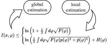
Figure 1: The bound for the mutual information $I(x,\varphi)$ in terms of Fisher information $F(\varphi)$ allows for the transfer of the results obtained for local estimation to global estimation.

To show the usefulness of our bounds, we apply them to a case study in quantum metrology. Quantum metrology [28, 29, 30, 31, 32, 33, 34, 35, 36] is the study of how quantum effects such as entanglement [28] or squeezing [37] can be used to enhance the precision of the measurement of a parameter $\varphi$ of a quantum system. In the noiseless case, it is easy to show that the ultimate limit in precision when the system is sampled $N$ times, the Heisenberg scaling $\Delta\varphi\propto 1/N$, can be achieved only using quantum effects, except in the trivial case in which a single probe samples the system repeatedly and is measured only once. Instead, classical strategies are limited to the standard quantum limit (SQL) $\Delta\varphi\propto 1/\sqrt{N}$ of the central limit theorem. In the noisy case [38, 39, 40, 41, 42, 43, 44, 45, 46] the situation is much more complicated, and, even though typically in the asymptotic regime of large $N$ the Heisenberg scaling cannot be achieved anymore, one can still obtain quantum enhancements by large factors. Most of these results have been obtained using Fisher information techniques, such as the quantum Cramer-Rao bound  [38, 40, 41, 42, 43, 44, 45, 46]. As we show below, our new bounds allow us to transfer the highly sophisticated results on FI in the presence of noise to the MI in a simple way. In the noisy case, this provides a nontrivial bridge between local and global quantum estimation strategies.

I Bounding mutual information by Fisher information

The estimation of a parameter $\varphi$ from measurements is described by two probabilities: the prior distribution of the parameter $p(\varphi)$ and the conditional probability $p(x|\varphi)$ of the measurement results $x$. Together they constitute the joint probability $p(x,\varphi)=p(x|\varphi)p(\varphi)$. The MI is $I(x,\varphi):=H(\varphi)-H(\varphi|x)$, where $H(\varphi)=-\int d\varphi\>p(\varphi){\ln}p(\varphi)$ is the entropy of $p(\varphi)$ and $H(\varphi|x)$ is the conditional entropy, given $x$. $I$ tells us the amount of information (in nats) about $\varphi$ obtained from $x$. The FI is given by $F(\varphi)=\sum_{x}\frac{1}{p(x|\varphi)}\left(\frac{dp(x|\varphi)}{d\varphi}\right)^{2}$ and tells us how much information on $\varphi$ is contained in $p(x|\varphi)$. The following two theorems relate MI to FI.

Theorem 1.

If $p(\varphi)$ has a finite support $\Theta$ (i.e. $\varphi$ is guaranteed to belong to a finite-size set $\Theta$), then

$$I(x,\varphi)\leq{\ln}\left(1+\frac{1}{2}\int_{\Theta}d\varphi\sqrt{F(\varphi)}\right).$$ (1)

This inequality holds for any $p(x|\varphi)$, so in the context of quantum metrology, by replacing the FI with the quantum Fisher information, one obtains a bound valid for any possible measurement. Note that the integral is invariant for reparametrization of the probabilities, since it is related to Jeffreys’ prior [47]. Indeed, the FI is known to define a metric corresponding to an Euclidean distance between $\sqrt{p(x|\varphi)}$ and $\sqrt{p(x|\varphi+d\varphi)}$ [48], so the above integral is just the size of $\Theta$ in this metric.

If the support of $p(\varphi)$ is not bounded, the following holds:

Theorem 2.

For arbitrary probability $p(\varphi)$, we have

$$I(x,\varphi)\leq{\ln}\left(\frac{1}{2}\int d\varphi\sqrt{F(\varphi)p(\varphi)^{2}+\dot{p}(\varphi)}\right)+H(\varphi),$$ (2)

where $\dot{p}=dp/d\varphi$ and the $\ln$ part is obviously an upper bound to $-H(\varphi|x)$. In contrast to the previous bound, this is not reparametrization invariant (indeed, it is well known that the differential entropy $H(\varphi)$ is defined modulo an arbitrary additive constant). So, the upper bound, and also its tightness, will depend on the parametrization.

Proof of the two bounds. Fix $\varphi$ and use the Cauchy-Schwarz inequality considering $\frac{\dot{p}(x,\varphi)^{2}}{p(x,\varphi)}$ and $p(x,\varphi)$ as vectors (functions of $x$). One gets (App. A):

$${\textstyle\sum_{x}}|\dot{p}(x,\varphi)|\leq\sqrt{F(\varphi)p(\varphi)^{2}+\dot{p}(\varphi)}.$$ (3)

Since $p(\varphi)$ is normalized, it goes to $0$ for $\varphi\to\pm\infty$, so

$$\sum_{x}\max_{\varphi}p(x,\varphi)\leq\frac{1}{2}\int d\varphi\sum_{x}|\dot{p}(x,\varphi)|.$$ (4)

Let $\bar{p}_{x}=\int d\varphi\>p(x|\varphi)p(\varphi)$. From the definition of $H(\varphi|x)$:

$$-H(\varphi|x)=\sum_{x}\int d\varphi\>p(x,\varphi){\ln}\left(\frac{p(x,\varphi)}{\bar{p}_{x}}\right)\leq\\ {\textstyle\sum_{x}}\bar{p}_{x}{\ln}\left({\max_{\varphi}p(x,\varphi)}/{\bar{p}_{x}}\right)\leq{\ln}{\textstyle\sum_{x}}\max_{\varphi}p(x,\varphi),$$ (5)

where the last inequality is obtained by replacing $\bar{p}_{x}$ by free parameters $q_{x}$ (with $\sum_{x}q_{x}=1$) and performing direct maximization. Combining the above three inequalities, we obtain $-H(\varphi|x)\leq{\ln}\left(\frac{1}{2}\int d\varphi\sqrt{F(\varphi)p(\varphi)^{2}+\dot{p}(\varphi)}\right)$, which, adding $H(\varphi)$ to both members, implies Eq. (2).

Now we derive Eq. (1) from Eq. (2). First note, that from general property $\sqrt{x+y}\leq\sqrt{x}+\sqrt{y}$, the expression $\frac{1}{2}\int d\varphi\sqrt{F(\varphi)p(\varphi)^{2}+\dot{p}(\varphi)^{2}}$ may be further bounded by

$$\leq\frac{1}{2}\int d\varphi\sqrt{F(\varphi)p(\varphi)^{2}}+\frac{1}{2}\int d\varphi\sqrt{\dot{p}(\varphi)^{2}}.$$ (6)

Next, we can always transform the parameter $\varphi$ to $\varphi^{\prime}=\int_{-\infty}^{\varphi}d\varphi^{\prime\prime}p(\varphi^{\prime\prime})$, which is uniformly distributed in $[0,1]$ and $0$ outside.Then the derivative of a probability distribution is $\delta(\varphi^{\prime})-\delta(\varphi^{\prime}-1)$, so the last term in Eq. (6) is equal $1$. Moreover, $H(\varphi^{\prime})=0$, so finally:

$$I(x,\varphi^{\prime})\leq{\ln}\left(1+\frac{1}{2}\int_{0}^{1}d\varphi^{\prime}\sqrt{F(\varphi^{\prime})}\right).$$ (7)

Both sides of the above inequality are invariant for reparametrization (up to changing the limits of the integral). Therefore, after proving this inequality in peculiar parametrization, we can go back to the initial one, so we get Eq. (1). $\square$

See also App. B for the discussion about potential tightening the bound by introducing additional variational function $f(\varphi)$.

II From local to global estimation

Here we will discuss how the bound for MI implies the bounds in global estimation, providing an alternative to the van Trees inequality. To derive the van Trees inequality [11] one can use the Efroimovich relation [7] (see also [8, 9]):

$$\begin{split}\frac{1}{2\pi e}e^{2H(\varphi|x)}\geq&\frac{1}{\int d\varphi F(\varphi)p(\varphi)+P},\\ {\rm with}\quad&P=\int d\varphi\frac{1}{p(\varphi)}\left(\frac{dp(\varphi)}{d\varphi}\right)^{2},\end{split}$$ (8)

where $P$ can be interpreted as the information included in the prior. Indeed, the Bayesian quadratic cost is related to mutual information via [49, 12]:

$$\overline{\Delta^{2}\tilde{\varphi}}\geq\frac{e^{2H(\varphi|x)}}{2\pi e}=\frac{e^{2H(\varphi)}e^{-2I(x,\varphi)}}{2\pi e},$$ (9)

where $\overline{\Delta^{2}\tilde{\varphi}}:=\int d\varphi\>p(\varphi)\int d\tilde{\varphi}\>p(\tilde{\varphi}|\varphi)(\tilde{\varphi}-\varphi)^{2}$. Introducing Efroimovich’s inequality Eq. (8) into Eq. (9) we find the van Trees one:

$$\overline{\Delta^{2}\tilde{\varphi}}\geq\frac{1}{\int d\varphi\>F(\varphi)p(\varphi)+P}.$$ (10)

Alternatively, by applying our Eq. (1) we obtain

$$\overline{\Delta^{2}\tilde{\varphi}}\geq\frac{e^{2H(\varphi)}}{2\pi e}\frac{1}{(1+\frac{1}{2}\int_{\Theta}d\varphi\>\sqrt{F(\varphi)})^{2}}.$$ (11)

Here the prior information is included via $H(\varphi)$ in the exponent and via the range of the integral in the denominator. In particular, for the relevant case of a rectangle prior of width $d$ with FI constant over the prior, one still obtains a significant bound, contrary to the van Trees case where $P$ diverges (see below):

$$\overline{\Delta^{2}\tilde{\varphi}}\geq\frac{2}{\pi e}\frac{1}{(2/d+\sqrt{F})^{2}}.$$ (12)

As expected, in the limit of many repetitions $N$ of the estimation procedure, the prior knowledge becomes irrelevant, since $F$ typically grows linearly with $N$. A disadvantage of this bound is that it is not asymptotically tight, because of the multiplicative factor $2/\pi e$.

Of course, a further bound for the Bayesian cost can be obtained also for unbounded-support $p(\varphi)$ by inserting Eq. (2) into Eq. (9):

$$\overline{\Delta^{2}\tilde{\varphi}}\geq\frac{2}{\pi e}\frac{1}{(\int d\varphi\sqrt{F(\varphi)p(\varphi)^{2}+\dot{p}(\varphi)^{2}})^{2}},$$ (13)

which, for example, for Gaussian priors leads to a bound qualitatively similar to the van Trees one (see App. C).

Our results (11) and (13) provide bounds to the quadratic Bayesian cost. But a relation similar to Eq. (9) may be derived for any moment (see Lemma B.1. in [24]). Therefore, our bounds to MI imply a bound for the Bayesian cost with an arbitrary cost function, assuming that it may be expanded in the Taylor series. These show that the bound for MI is more informative than any bound to Bayesian cost.

III Relation to the Efroimovich inequality

Here we compare our bounds with Efroimovich’s inequality (8). Using the definition of MI, $I=H(\varphi)-H(\varphi|x)$, it immediately gives:

$$I(x,\varphi)\leq\frac{1}{2}\ln\left[\frac{1}{2\pi e}\left(\int d\varphi F(\varphi)p(\varphi)+P\right)\right]+H(\varphi).$$ (14)

Assuming that $P$ does not diverge, and that the probability $p(x,\varphi)$ is not degenerate (i.e. $\forall_{\varphi^{\prime}\neq\varphi}p(x,\varphi^{\prime})\not=p(x,\varphi)$), then (8) and (14) are tight asymptotically in the number of repetitions $N$ of the estimation, and saturable using the maximum likelihood estimator. Indeed, first, FI increases linearly with $N$, so asymptotically the impact of $P$ in the upper bound becomes negligible. Second, from the asymptotic normality of the maximum likelihood estimator, we have

$$H(\varphi|\tilde{\varphi}_{\textrm{M}L})\to-\frac{1}{2}\ln\left[\frac{1}{2\pi e}\int d\varphi F(\varphi)p(\varphi)\right].$$ (15)

Third, assigning the estimator’s value to the measurement result $\tilde{\varphi}_{\textrm{M}L}(x)$ may only decrease the MI, namely $I(\tilde{\varphi}_{\textrm{M}L},\varphi)\leq I(x,\varphi)$. This lower bound, through (15) converges to the upper bound Eq. (14).

While for Gaussian prior the quantity $P$ is a reasonable measure of information (the inverse of the variance), it is completely unreasonable for the rectangle distribution, where $P$ diverges. In general, $P$ depends more on the sharpness of distribution on its edges than on its actual width, which is more an artifact of the derivation of the bound, rather than a well-motivated feature. Overcoming this problem was also discussed in [8, 9].

This issue does not appear in our bounds (1) and (2). Indeed, from (6) it follows that the impact of $\dot{p}(\varphi)$ can be bounded by $\frac{1}{2}\int d\varphi|\dot{p}(\varphi)|$. In particular, for any prior concentrated around one region (more formally: the region where the derivative $\dot{p}(\varphi)$ changes its sign only once), it may be bounded by constant $+1$, no matter how sharply the prior changes. Also the bound (2) is not asymptotically tight, because of the multiplicative factors inside the $\ln$.

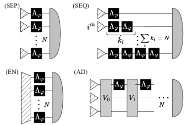
Figure 2: Different possible quantum estimation schemes: $N$ elementary gates (black boxes) are used on separably prepared probes in SEP; in a sequential manner in SEQ; starting from an entangled input state (shaded box) in EN; in an adaptive way in AD ($V_{i}$ representing joint unitaries). Each subsequent one includes all previous ones as special cases. The gray cups on the right represent a (possibly joint) measurement.

IV Applying bound to quantum metrology

To show the usefulness of the newly derived bounds, we now show how they can be used to give bounds to noisy quantum metrology for mutual information.

Consider the $\varphi$-dependent CPTP map $\Lambda_{\varphi}[\cdot]$ that noisily encodes the parameter $\varphi$ onto a quantum probe. The probability distribution of the final measurement output is given via the Born rule $p(x|\varphi)=\mathrm{Tr}(\rho_{\varphi}M_{x})$, where $\rho_{\varphi}$ is the final state and $M_{x}$ is a POVM element ($M_{x}\geq 0$, $\sum_{x}M_{x}=\openone$). The phase estimation problem is a typical example. Consider the simple case of qubit probes, where the parameter $\varphi$ is encoded through a unitary $U_{\varphi}=\ket{0}\bra{0}+e^{i\varphi}\ket{1}\bra{1}$, followed by some kind of noise (e.g. dephasing, erasing) which together constitute the map $\Lambda_{\varphi}[\cdot]$. Note, that in this model $\varphi\in[0,2\pi[$, and the Efroimovich’s inequality cannot be applied to a uniform prior.

We consider the action of $N$ such gates in the configurations shown in Fig. 2. The most basic strategy is to use all gates separately (SEP). The next step is to allow them to be divided into groups to be used sequentially (SEQ). More generally, we can consider an entangled input state (EN). EN is strictly more powerful than the SEQ. In fact, any $k_{i}$ sequential usage of gates is equivalent to a single action on a N00N state with $k_{i}$ elements, where a gate acts on each of the entangled systems (in parallel). Even more powerful is the adaptive scheme (AD), which allows for an arbitrary input state entangled with an ancilla of arbitrary size and then a sequential action of $N$ gates interspersed by unitary controls. By choosing suitable SWAP gates as unitary controls, one may easily simulate EN, proving that AD is more powerful. Moreover, AD also can implement any partial measurement and any adaptive scheme (feed-forward) during the evolution.

In [15] the Heisenberg Scaling (HS) for MI has been defined as $I\propto{\ln}N$ and the standard quantum limit as $I\propto\frac{1}{2}{\ln}N$ (in analogy to the scaling of RMSE $\Delta\varphi\propto 1/N$ and $\Delta\varphi\propto 1/\sqrt{N}$ respectively). In the case of noiseless estimation, it is known that SEP allows at most standard quantum limits, while SEQ is enough for obtaining HS via QPEA algorithm [15] (which implies, that it may be obtained by EN and AD as well). However, the noisy case has not been discussed up to now while using MI as a figure of merit.

We can now apply the bounds derived above, e.g. Eq. (1), to transfer the highly nontrivial theory of noisy-channel estimation theory from the FI to the MI formalism. For FI, the general necessary and sufficient conditions for the obtainability of HS in the estimation of a given channel are known, expressed in terms of Kraus operators [43, 46, 45] or Lindblad operators [44, 50]. Moreover, the resulting bounds are known to be saturable in the asymptotic limit $N\to\infty$ of many gates [45]. For example, for a mentioned model of phase estimation, it was shown that in the presence of dephasing or erasing noise, the FI obtainable by any protocol involving $N$ gates is bounded from above by $F\leq N\eta/(1-\eta)$ [43], where $\eta$ is the noise parameter ($\eta\to 1$ in the noiseless case, $\eta\to 0$ for maximum noise). Applying this bound to Eq. (1) we immediately find $I(x,\varphi)\leq{\ln}(1+\pi\sqrt{N}\sqrt{\eta/(1-\eta)})$. This holds even for the most general scheme AD. Even if the bound is not tight (there is an additive constant gap), it implies a standard quantum limit asymptotic scaling for all $\eta<1$, and also gives the scaling with the intensity of the noise (see App. D for more details). Similar results can be obtained easily using different bounds to FI [40, 41, 42]. Naturally, this does not rule out quantum enhancements: for sufficiently large $\eta$ one might still find an arbitrarily large constant gain over the SQL.

These will provide only the upper bounds to MI and so they can only be used to exclude the possibility of attaining the HS, but never to prove its achievability. While there exist lower bounds on the MI expressed in terms of the FI in the literature, they all require additional assumptions and a general discussion is impossible. In the noiseless case, it may be exemplified by the N00N state which allows the HS for the FI, but not for the MI, due to its periodicity with period $1/N$ (indeed, irrespectively of the value of $\varphi$, the N00N state belongs to a two-dimensional subspace of the full Hilbert space, so it can carry at most one bit of information $I\leqslant{\ln}(2)$).

V Conclusions

In conclusion, we have derived two bounds, Eqs. (1) and (2) for the MI in terms of the FI. We used these bounds to give two extensions of the van Trees inequality, Eqs. (11) and (13). We discussed the relation of all these bounds to the Efroimovich inequality (8). To prove the usefulness of these bounds, we have showed that they can be used to extend to the MI-based quantum metrology many highly nontrivial results known for the FI case.

Appendix A Derivation of inequality (3)

Here we derive Eq. (3). By Cauchy’s inequality,

$$\sum_{x}\left|\dot{p}(x,\varphi)\right|=\sum_{x}\sqrt{\frac{\left[\dot{p}(x,\varphi)\right]^{2}}{p(x,\varphi)}}\sqrt{p(x,\varphi)}$$ (16)

$$\leq\sqrt{\sum_{x}\frac{\left[\dot{p}(x,\varphi)\right]^{2}}{p(x,\varphi)}}\sqrt{\sum_{x}p(x,\varphi)}$$

$$=\sqrt{\sum_{x}\frac{\left[\dot{p}(x,\varphi)\right]^{2}}{p(x|\varphi)p(\varphi)}}\sqrt{p(\varphi)}$$

$$=\sqrt{\sum_{x}\left[\frac{\dot{p}(x|\varphi)^{2}}{p(x|\varphi)}p(\varphi)^{2}+2\dot{p}(x|\varphi)p(\varphi)\dot{\rho}(\varphi)+p(x|\varphi)\dot{p}(\varphi)^{2}\right]}$$

$$=\sqrt{F(\varphi)p(\varphi)^{2}+\dot{p}(\varphi)^{2}},$$

where we used $\sum_{x}p(x|\varphi)=1$ and $\sum_{x}\dot{p}(x|\varphi)=0$.

Appendix B Generalization of Theorems 1, 2

Here we will discuss a generalization of Theorems 1, 2. In analogy to Eq. (16), from Cauchy’s inequality for vectors $\sqrt{\left|\frac{d(p(x|\varphi)f(\varphi))}{d\varphi}\right|\frac{1}{p(x|\varphi)f(\varphi)}}$ and $\sqrt{p(x|\varphi)f(\varphi)}$ with arbitrary positive function $f(\varphi)$ we obtain:

$$\sum_{x}\left|\frac{d(p(x|\varphi)f(\varphi))}{d\varphi}\right|\leq\\ \sqrt{F(\varphi)f(\varphi)^{2}+\dot{f}(\varphi)^{2}}.$$ (17)

If $f(\varphi)$ goes to $0$ for $\varphi\to\pm\infty$, we have:

$$\sum_{x}\max_{\varphi}p(x|\varphi)f(\varphi)\leq\frac{1}{2}\int d\varphi\sum_{x}\left|\frac{d(p(x|\varphi)f(\varphi))}{d\varphi}\right|.$$ (18)

Next, the mutual information may be written as:

$$I(x,\varphi)=\sum_{x}\int d\varphi\>p(x,\varphi)\ln\frac{p(x,\varphi)}{p(x)p(\varphi)}=\\ \sum_{x}\int d\varphi\>p(x,\varphi)\ln\frac{p(x|\varphi)f(\varphi)}{p(x)}-\sum_{x}\int d\varphi\>p(x,\varphi)\ln f(\varphi),$$ (19)

where the first element may be bounded by:

$$\sum_{x}\int d\varphi\>p(x,\varphi)\ln\frac{p(x|\varphi)f(\varphi)}{p(x)}\leq\\ \sum_{x}p(x)\ln\max_{\varphi}\frac{p(x|\varphi)f(\varphi)}{p(x)}\leq\\ \ln\sum_{x}\max_{\varphi}p(x|\varphi)f(\varphi).$$ (20)

Combining all above one may get:

$$I(x,\varphi)\leq\ln\left(\frac{1}{2}\int d\varphi\sqrt{F(\varphi)f(\varphi)^{2}+\dot{f}(\varphi)^{2}}\right)+\\ -\int d\varphi\>p(\varphi)\ln f(\varphi),$$ (21)

which may be further optimized over choice $f(\varphi)$ (going to zero for $\varphi\to\pm\infty)$. Note especially, that for $f(\varphi)$ being flat on $[0,1]$, we obtain Eq. (1), while for $f(\varphi)=p(\varphi)$, we get Eq. (2).

Appendix C Applying the bound for Gaussian distribution

Consider an a priori distribution $p(\varphi)=\frac{1}{\sqrt{2\pi\sigma^{2}}}\exp(-\frac{\varphi^{2}}{2\sigma^{2}})$. Substituting Eq. (2) into Eq. (9) we obtain:

$$\overline{\Delta^{2}\tilde{\varphi}}\geq\frac{2}{\pi e}\frac{1}{(\int d\varphi\sqrt{F(\varphi)+\varphi^{2}/\sigma^{4}}p(\varphi))^{2}}.$$ (22)

Further, assuming that $F(\varphi)$ does not change with $\varphi$, the integral may be calculated analiticaly as $\frac{\sqrt{2}}{\sigma}U[-\frac{1}{2},0,\frac{F\sigma^{2}}{2}]$, where $U(\cdot)$ is Tricomi confluent hypergeometric function.

For a slightly less tight, but simpler bound, note that after introducing the variable $\eta=\varphi^{2}$, the quantity $\sqrt{F+\eta/\sigma^{4}}$ is concave as a function of $\eta$, so $\mathbb{E}[\sqrt{F+\eta/\sigma^{4}}]\leq\sqrt{F+\mathbb{E}[\eta]/\sigma^{4}}$ (with $\mathbb{E}[\cdot]$ denoting averaging), so the integral may be bounded from above by $\sqrt{F+1/\sigma^{2}}$ (numerical results also show that this is a good approximation for the exact result for $F\sigma^{2}\gg 1$). For any $F,\sigma$ we have:

$$\overline{\Delta^{2}\tilde{\varphi}}\geq\frac{2}{\pi e}\frac{1}{F+1/\sigma^{2}},$$ (23)

while from the van Trees inequality we have Eq. (10):

$$\overline{\Delta^{2}\tilde{\varphi}}\geq\frac{1}{F+1/\sigma^{2}}.$$ (24)

Then, for this specific case, our bound is less tight, because of the $2/\pi e$ multiplicative factor.

Appendix D Mutual information in occurrence of noise

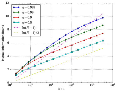
Figure 3: The mutual information bound given by Eq. (1) with maximum Fisher information, for the dephasing channel and amplitude damping channel. The two dashed lines help to compare the bound with HS and SQL.

We now give a global bound to the mutual information in terms of $N$, the number of calls to the phase gate $U_{\varphi}=\ket{0}\bra{0}+e^{i\varphi}\ket{1}\bra{1}$, in the presence of dephasing and amplitude damping noise.

In our noise model, each unitary gate $U_{\varphi}$ is replaced by the noisy gate acting on the density operator as,

$$\Lambda_{\varphi}:\rho\mapsto\sum_{k}K_{k}U_{\varphi}\rho U_{\varphi}^{\dagger}K_{k}^{\dagger},$$ (25)

with $K_{k}$ being the Kraus operators.

For dephasing noise the Kraus operators are,

$$K_{0}=\openone\left(\frac{1+\sqrt{\eta}}{2}\right)^{1/2},\qquad K_{1}=\sigma_{z}\left(\frac{1-\sqrt{\eta}}{2}\right)^{1/2},$$ (26)

where $\openone=\ket{0}\bra{0}+\ket{1}\bra{1}$, $\sigma_{z}=\ket{0}\bra{0}-\ket{1}\bra{1}$, and $\eta$ is the noise parameter. Also, the Kraus operators in the presence of amplitude damping noise are,

$$K_{0}=\begin{pmatrix}1&0\\ 0&\sqrt{\eta}\end{pmatrix},\quad K_{1}=\begin{pmatrix}0&\sqrt{1-\eta}\\ 0&0\end{pmatrix}.$$ (27)

Finally, for erasing noise the Kraus operators are,

$$\begin{gathered}K_{0}=\begin{pmatrix}\sqrt{\eta}&0&0\\ 0&\sqrt{\eta}&0\\ 0&0&0\end{pmatrix},\quad K_{1}=\begin{pmatrix}0&0&0\\ 0&0&0\\ 0&0&1\end{pmatrix},\\ K_{2}=\begin{pmatrix}0&0&0\\ 0&0&0\\ \sqrt{1-\eta}&0&0\end{pmatrix},\quad K_{3}=\begin{pmatrix}0&0&0\\ 0&0&0\\ 0&\sqrt{1-\eta}&0\end{pmatrix},\end{gathered}$$ (28)

where a third dimension is added to indicate loss of phase information.

In this notation, an asymptotic upper bound to the Fisher information is [43, 46],

$$F\leq NF_{\mathrm{as}},$$ (29)

where $F_{\mathrm{as}}=\eta/(1-\eta)$ for both dephasing and erasure noise with the most general AD strategy, as well as amplitude damping noise with EN strategy [42]. Combining the Fisher information bound with Eq. (1), we get a global upper bound to the mutual information,

$$I(x,\varphi)\leq\ln\left(1+\pi\sqrt{\frac{N\eta}{1-\eta}}\right).$$ (30)

For amplitude damping noise, the Fisher information bound is slightly different, and the mutual information bound can be derived similarly.

Especially, when limited to the EN strategy, a tighter bound to Fisher information for finite-$N$ is given by [51],

$$F\leq\frac{NF_{\mathrm{as}}}{1+\frac{F_{\mathrm{as}}}{N}}.$$ (31)

Combining the Fisher information bound with Eq. (1), we get a global upper bound to the mutual information,

$$I(x,\varphi)\leq\ln\left(1+\pi\sqrt{\frac{N\eta/(1-\eta)}{1+\eta/N(1-\eta)}}\right),$$ (32)

for all these three noise models. We plot the right hand side of Eq. (32) in Fig. 3, in which we can see a transition from the HS to the SQL as $N$ increases. The stronger the noise is, the earlier the transition happens.