Non-adiabatic particle production scenario in algebraically coupled quintessence field with dark matter fluid

Abstract

We investigate the dynamics of an algebraically coupled quintessence field with a dark matter fluid, considering a scenario involving non-adiabatic particle production, through the action principle by modifying the interaction Lagrangian. The interaction parameter serves as the source of dark matter particle and entropy production. As particle creation occurs due to the interaction between the field and fluid sectors, the system manifests an additional pressure. Our analysis includes studying the system’s dynamics by considering an exponential type of interaction corresponding to the field’s exponential potential. We find that the system exhibits phantom behavior at the current epoch before stabilizing in the accelerating future epoch of the universe.

I Introduction

Over the past two decades, observations have shed light on the dynamics of the cosmos at its largest scale, revealing evidence that the expansion of the universe is accelerating [1, 2, 3, 4, 5, 6, 7, 8, 9]. One of the most accepted explanations for this late-time cosmic acceleration is the existence of an exotic component known as the cosmological constant ($\Lambda$), which exerts negative pressure. The largest portion of the universe’s energy budget consists of the cosmological constant, accounting for about $70\%$. Additionally, approximately $25\%$ of the energy budget is dominated by a non-relativistic, pressureless fluid commonly referred to as dark matter, with the remaining portion composed of baryonic matter.

Although the $\Lambda$CDM model, where CDM represents cold dark matter, is favored due to its ability to describe most observational evidence, it faces several theoretical shortcomings, including the cosmological constant problem, fine-tuning issues, and the cosmological coincidence problem [10, 11, 12, 13, 14, 15, 16]. Numerous alternatives have been proposed to address these issues, either by modifying the gravitational sector [17, 18, 19, 20] or by modifying the matter sector [21, 22, 23, 24, 25, 26, 27]. In many instances, scalar fields serve as viable candidates for dark energy (DE) and are often minimally coupled with pressureless dark matter (DM) fluid. However, beyond their gravitational signatures, these enigmatic forms of matter pose puzzles to the scientific community. Consequently, numerous possible scenarios have been intensely investigated, including (i) non-gravitational interactions between dark matter and dark energy [28, 29, 30, 31, 32, 33, 34] and (ii) non-minimal coupling between matter fields and curvature [35, 36, 37, 38, 39, 40, 41, 42, 43, 44, 45, 46, 47].

A recent approach has emerged to investigate the non-gravitational interaction between dark sectors through the variational principle [40, 41, 48]. In these studies, dark energy is governed by a scalar field, while the action for the dark matter fluid is modeled using the relativistic fluid action proposed by Brown [49]. This action encompasses the energy density of the fluid $\rho$, the particle flux number $J^{\mu}$, and several Lagrange multipliers. Additionally, a non-gravitational interaction term is introduced at the action level, consisting of fluid and field variables, denoted by $\mathcal{L}_{\rm int}=-\sqrt{-g}f(n,s,\phi)$, where $f$ is an arbitrary interaction function depending on the fluid number density $n$, entropy per particle $s$, and scalar field $\phi$. One immediate constraint studied under these models is the conservation of number density $\nabla_{\mu}(nu^{\mu})=0$, where $u^{\mu}$ represents the fluid’s four-velocity, and the conservation of entropy $\nabla_{\mu}(snu^{\mu})=0$. Consequently, the normal component of the fluid’s covariant derivative of the energy-momentum tensor vanishes, i.e., $u_{\mu}\nabla_{\nu}T^{\mu\nu}=0$, implying $\rho\propto a^{-3}$, where $a$ is the scale factor. However, the inclusion of $\phi$ in the interacting Lagrangian modifies the field evolution, resulting in dynamics different from the minimally coupled scenario. In light of the current cosmological crisis, where the discrepancy between the measured values of the Hubble parameter $H_{0}$ and the amplitude of matter density $S_{8}$ between high and low-redshift data exceeds the $4.4\sigma$ level [50, 51, 52], exploring scenarios where both the field and fluid sectors are simultaneously affected becomes crucial.

This paper explores a scenario where the dynamics between the quintessence field and dark matter fluid are investigated by modifying the interaction Lagrangian $f(n,s,\phi)\rightarrow f(n,s,\phi,\varphi)$, where $\varphi$ is a fluid Lagrange multiplier. This modification results in alterations to the thermodynamic constraints such that $\nabla_{\mu}(nu^{\mu})\neq 0$ and $\nabla_{\mu}(snu^{\mu})\neq 0$. With the number density of the dark matter fluid no longer conserved, energy flow from the quintessence field to the dark matter can lead to the creation of matter particles, consequently inducing an additional pressure known as creation pressure $P_{c}$ [53, 54, 55, 56, 57, 58]. By analyzing this scenario from the action principle, the interaction function serves as a source of particle and entropy production. We obtained the fluid’s equations of motion and temperature evolution from thermodynamic principles. Additionally, we provide a background dynamics by considering an exponential type of interaction $f\propto\rho^{\beta}e^{\delta\kappa\phi+\gamma\varphi}$, corresponding to the field’s exponential potential. Stability analysis of the interacting system is conducted using the standard linearization technique [59, 60, 61, 62], with proper constraints on thermodynamic quantities to ensure positivity of entropy and number density throughout the evolution. Our findings indicate that the interacting system exhibits a stable accelerating critical point in the future epoch of the universe. However, at the present epoch $a=1$, the effective equation of state (EoS) crosses the phantom barrier, i.e., $\omega_{\rm eff}\leq-1$. Furthermore, we utilize $43$ Hubble data and $1701$ Pantheon+ data to numerically simulate the current model against the $\Lambda$CDM model, revealing compatibility with the data for $f\propto\rho^{3}$.

We organized the paper as follows: In sec. II, we set up the action for the algebraically coupled field-fluid system and obtained the governing background equations. In sec. III, we present brief thermodynamic relations corresponding to the fluid component. A detailed picture of the conservation of energy-momentum tensor is presented in sec. IV. The dynamical system’s stability is discussed in sec. V. Finally, a brief conclusion is outlined in sec. VI.

II Action for the algebraic interaction

The action describing the algebraically (non-minimally) coupled field-fluid scenario is given by [40]:

$$S=\int_{\Omega}d^{4}x\sqrt{-g}\frac{R}{2\kappa^{2}}-\sqrt{-g}\rho(n,s)+J^{\mu}(\varphi_{,\mu}+s\theta_{,\mu}+\alpha_{A}{\beta}_{,\mu}^{A})-\sqrt{-g}\mathcal{L}_{\phi}(\phi,\partial{}_{\mu}\phi)-\alpha_{1}\sqrt{-g}f(n,s,\phi,\varphi),$$ (1)

where,

$$J^{\mu}=\sqrt{-g}nu^{\mu},\quad|J|=\sqrt{-g_{\mu\nu}J^{\mu}J^{\nu}},\quad n=\frac{|J|}{\sqrt{-g}},\quad u^{\mu}u_{\mu}=-1\,.$$ (2)

In this action, the first term corresponds to the Einstein-Hilbert action, where $g$ denotes the determinant of the metric tensor $g^{{\mu\nu}}$, $R$ represents the Ricci scalar, and $\kappa^{2}=8\pi G$. The second and third terms together represent the action for a relativistic fluid, where the energy density of the dark matter fluid is denoted as $\rho$, depending on the fluid number density $n$ and the entropy density per particle $s$. The relativistic fluid Lagrangian contains the fluid flux density $J^{\mu}$ and Lagrange multipliers $\varphi$, $\theta$, $\alpha^{A}$, $\beta_{A}$. Note that Greek indices range from 0 to 3, and $A$ runs from 1 to 3. It’s important to distinguish between $\alpha_{1}$ and $\alpha^{A}$ as they are distinct quantities unless specified. The commas followed by Greek indices indicate covariant derivatives. The field action is given by:

$$\mathcal{L}_{\phi}=\frac{1}{2}\partial{}_{\mu}\phi\partial{}^{\mu}\phi+V(\phi).$$ (3)

Here, the Lagrangian represents a standard quintessence field with the potential $V(\phi)$. The remaining term in the action corresponds to the interaction parameter $f$, which depends on fluid and field parameters, while $\alpha_{1}$ is a constant parameter. Taking the variation of the action Eq. (1) with respect to the metric $g^{{\mu\nu}}$ yields the Einstein field equation:

$$R_{{\mu\nu}}-\dfrac{1}{2}Rg_{{\mu\nu}}=\kappa^{2}\left(T_{{\mu\nu}}^{M}+T_{{\mu\nu}}^{\phi}+T_{{\mu\nu}}^{\rm int}\right).$$ (4)

Here, the stress tensor of the matter components is defined as $T_{{\mu\nu}}=\frac{-2}{\sqrt{-g}}\frac{\delta S}{\delta g^{{\mu\nu}}}$. The energy-momentum tensor corresponding to the relativistic fluid is:

$$T^{{\mu\nu}}_{M}=\rho u^{\mu}u^{\nu}+\left(n\frac{\partial{}\rho}{\partial{}n}-\rho\right)(u^{\mu}u^{\nu}+g^{{\mu\nu}}).$$ (5)

Similarly, corresponding to the interaction part:

$$T^{{\mu\nu}}_{\rm int}=\alpha_{1}fu^{\mu}u^{\nu}+\alpha_{1}\left(n\frac{\partial{}f}{\partial{}n}-f\right)(u^{\mu}u^{\nu}+g^{{\mu\nu}}).$$ (6)

The field’s stress tensor becomes:

$$T_{\phi}^{{\mu\nu}}=-g^{{\mu\nu}}\left(\frac{1}{2}\partial{}_{\alpha}\phi\partial{}^{\alpha}\phi+V(\phi)\right)+\partial{}^{\mu}\phi\partial{}^{\nu}\phi.$$ (7)

To evaluate the energy density and corresponding pressure of these matter components, we compare with the stress tensor for the perfect fluid $T^{{\mu\nu}}=\rho u^{\mu}u^{\nu}+P(g^{{\mu\nu}}+u^{\mu}u^{\nu})$. Hence, the energy density and pressure of the fluid become:

$$\rho_{M}=\rho,\quad P_{M}=\left(n\frac{\partial{}\rho}{\partial{}n}-\rho\right).$$ (8)

The energy density and pressure corresponding to the algebraic interaction become:

$$\rho_{\rm int}=\alpha_{1}f,\quad P_{\rm int}=\alpha_{1}\left(n\frac{\partial{}f}{\partial{}n}-f\right).$$ (9)

The field energy density and pressure become:

$$\rho_{\phi}=\frac{1}{2}\dot{\phi}^{2}+V(\phi),\quad P_{\phi}=\frac{1}{2}\dot{\phi}^{2}-V(\phi).$$ (10)

In the flat FLRW metric $ds^{2}=-dt^{2}+a(t)^{2}d\vec{x}^{2}$, the Friedmann equations become:

$$3H^{2} = \kappa^{2}(\rho_{M}+\rho_{\phi}+\rho_{\rm int}),$$ (11)

$$2\dot{H}+3H^{2} = -\kappa^{2}(P_{M}+P_{\phi}+P_{\rm int}).$$ (12)

Upon taking the variation of the action with respect to $\phi$, the field equation becomes:

$$\ddot{\phi}+3H\dot{\phi}+\dfrac{dV(\phi)}{d\phi}+\alpha_{1}\frac{\partial{}f}{\partial{}\phi}=0.$$ (13)

III Thermodynamic relations

In this section, we will examine the thermodynamic aspect of the fluid in light of interaction. Upon varying the action with respect to the fluid variables, the corresponding equations of motion become:

$$J^{\mu}: \qquad u_{\mu}\left(\frac{\partial{}\rho}{\partial{}n}+\alpha_{1}\frac{\partial{}f}{\partial{}n}\right)+\varphi_{,\mu}+s\theta_{,\mu}+\beta_{A}\alpha^{A}_{,\mu}=0,$$ (14)

$$s: \qquad-\left(\frac{\partial\rho}{\partial s}+\alpha_{1}\frac{\partial{}f}{\partial{}s}\right)+nu^{\mu}\theta_{,\mu}=0\,,$$ (15)

$$\varphi: \qquad\nabla_{\mu}(nu^{\mu})+\alpha_{1}\dfrac{\partial{}f}{\partial{}\varphi}=0\,,$$ (16)

$$\theta: \qquad(sJ^{\mu})_{,\mu}=0\,,$$ (17)

$$\beta_{A}: \qquad J^{\mu}\alpha^{A}_{,\mu}=0\,,$$ (18)

$$\alpha^{A}: \qquad(\beta_{A}J^{\mu})_{,\mu}=0.$$ (19)

Due to the modifications in the interaction parameter, which now includes the Lagrange parameter $\varphi$, the number density of the fluid from Eq. (16) is no longer conserved, and the interaction parameter $f$ acts as a source of fluid particle number density. In the flat FLRW background metric, this equation reads as:

$$\dot{n}+3nH=-\alpha_{1}\frac{\partial{}f}{\partial{}\varphi}.$$ (20)

As the non-minimal coupling acts as a source of the fluid’s particle density, the corresponding contribution in entropy from Eq. (17) becomes:

$$\dot{s}=\frac{s}{n}\alpha_{1}\frac{\partial{}f}{\partial{}\varphi}$$ (21)

Therefore, due to the dependence of $\varphi$ in the interaction function, the fluid particle density may increase or decrease, resulting in a change in entropy. Consequently, the evolution of the fluid sector becomes non-adiabatic. As the interaction parameter induces changes in number density and entropy, the corresponding change in energy density of the fluid sector can be explored using the thermodynamic relation:

$$d(\rho V)=dQ-PdV.$$ (22)

Here, $dQ$ denotes the heat received by the fluid sector during time $dt$, and $V=a^{3}$ signifies the comoving volume. For the closed system, the above relation can be re-expressed as:

$$d(\rho/n)=Tds-Pd(1/n).$$ (23)

Here, $dq=dQ/N$, $n=N/V$, $s=S/N$, and $T=\frac{1}{n}\frac{\partial\rho}{\partial s}\big{|}_{n}$ is the temperature of the fluid [54]. As the particle production takes place, the system can absorb heat. The above relation can then be extended to the open system as:

$$d(\rho V)=TV(d(sn)-sdn)-PdV+\frac{\rho+P}{n}d(nV).$$ (24)

On differentiating both sides with respect to time $t$, we obtain:

$$\dot{\rho}+3H(\rho+P)=Ts\alpha_{1}\frac{\partial{}f}{\partial{}\varphi}-\alpha_{1}\frac{\rho+P}{n}\frac{\partial{}f}{\partial{}\varphi}.$$ (25)

From this, we can express the creation pressure or non-minimally induced pressure $P_{c}$ as:

$$P_{c}=\frac{1}{3H}\left(\frac{\rho+P}{n}-\frac{s}{n}\frac{\partial{}\rho}{\partial{}s}\right)\alpha_{1}\frac{\partial{}f}{\partial{}\varphi}.$$ (26)

Therefore, as the fluid’s particle number density changes, the system can exhibit an additional pressure known as creation pressure. The density evolution can be rewritten as:

$$\dot{\rho}+3H(\rho+P+P_{c})=0.$$ (27)

From Eq. (20) and Eq. (21), it is clear that if $\alpha_{1}\frac{\partial f}{\partial\varphi}<0$, the interaction contributes to an increment in the number density of the fluid particles. As a consequence, the change in entropy corresponding to the fluid sector decreases. Although the entropy of the matter sector decreases, it’s important to note that the entropy of the system as a whole may not decrease. Hence, the second law of thermodynamics for the entire system remains intact.

Using the above equation, the evolution of the temperature $T$ of the fluid can be determined. We utilize the total derivative of energy density as:

$$d\rho(n,T)=\left(\frac{\partial{}\rho}{\partial{}n}\right)_{T}dn+\left(\frac{\partial{}\rho}{\partial{}T}\right)_{n}dT,$$ (28)

After taking the time derivative and using equations Eq. (27) and Eq. (20), we obtain:

$$\dot{T}=\frac{1}{\left(\partial{}\rho/\partial{}T\right)_{n}}\left(-3H(\rho+P+P_{c})-\left(\frac{\partial{}\rho}{\partial{}n}\right)_{T}\dot{n}\right).$$ (29)

To evaluate $\left(\frac{\partial\rho}{\partial n}\right)_{T}$, we use the thermodynamic relation:

$$ds=\frac{1}{nT}d\rho-\frac{\rho+P}{n^{2}T}dn,$$ (30)

and using the partial derivative property, we obtain:

$$\left(\frac{\partial{}s}{\partial{}n}\right)_{T}=\frac{1}{nT}\left(\left(\frac{\partial{}\rho}{\partial{}n}\right)_{T}-\frac{\rho+P}{n}\right),\quad\left(\frac{\partial{}s}{\partial{}T}\right)_{n}=\frac{1}{nT}\left(\frac{\partial{}\rho}{\partial{}T}\right)_{n}.$$ (31)

Further using the property $\frac{\partial{}^{2}s}{\partial{}T\partial{}n}=\frac{\partial{}^{2}s}{\partial{}n\partial{}T}$, we get:

$$h=\rho+P=n\left(\frac{\partial{}\rho}{\partial{}n}\right)_{T}+T\left(\frac{\partial{}P}{\partial{}T}\right)_{n}\,.$$ (32)

Here, $h$ is the enthalpy per unit volume. Inserting this relation into $\dot{T}$ and using $\frac{(\partial{}P/\partial{}T)_{n}}{(\partial{}\rho/\partial{}T)_{n}}\equiv(\partial{}P/\partial{}\rho)_{n}$, we finally obtain:

$$\dot{T}/T=\frac{s\alpha_{1}\partial{}f/\partial{}\varphi}{(\partial{}\rho/\partial{}T)_{n}}+\frac{\dot{n}}{n}\left(\frac{\partial{}P}{\partial{}\rho}\right)_{n}.$$ (33)

Using Eq. (21), this relation is similar to the one that has been obtained in ref. [63]. The first term on the right-hand side shows the contribution from the non-conserved entropy of the fluid. To find the temperature evolution, we choose the model corresponding to the pressureless non-relativistic fluid. The energy density of the non-relativistic ideal gas $(k_{\rm B}=1)$ is:

$$\rho=Mn+\frac{3}{2}nT,$$ (34)

where $M$ is the mass of gas particles. Corresponding to this ideal gas model, the pressure, $P=n(\partial\rho/\partial n)-\rho=0$, vanishes. Using this relation, the temperature relation simplifies to:

$$\dfrac{\dot{T}}{T}=\dfrac{2\dot{s}}{3}.$$ (35)

This gives the variation of temperature with entropy irrespective of any form of interaction parameter $f$. Hence the entropy becomes:

$$s=s_{0}+\frac{3}{2}\ln(T/T_{0}).$$ (36)

Here, the parameters with subscript $0$ are integration constants representing the present value of the respective parameters.

IV Conservation of energy momentum tensor

In the preceding section, we explored the thermodynamic behavior of the fluid sector, employing thermodynamic relations to determine the corresponding evolution of fluid density. In this section, we delve into evaluating the covariant derivative of the stress tensor of the entire system to investigate the transportation of energy flow between the fluid and field sectors. To do so, we first redefine the matter stress tensor as:

$$T^{{\mu\nu}}_{A}=(\rho+\alpha_{1}f)u^{\mu}u^{\nu}+\left(n\frac{\partial{}\rho}{\partial{}n}-\rho+\alpha_{1}n\frac{\partial{}f}{\partial{}n}-\alpha_{1}f\right)(u^{\mu}u^{\nu}+g^{{\mu\nu}}).$$ (37)

With this redefinition, the Einstein tensor becomes $G_{{\mu\nu}}=\kappa^{2}(T_{{\mu\nu}}^{A}+T_{{\mu\nu}}^{\phi})$ . Upon taking the covariant derivative of the stress tensor, we obtain:

$$\nabla_{\mu}T^{\mu 0}_{A}=\dot{\rho}+\alpha_{1}\dot{f}+3H(\rho+\alpha_{1}f+P_{M}+P_{\rm int})=Q^{0}.$$ (38)

Utilizing Eq. (20) and Eq. (21), we can express:

$$\nabla_{\mu}T^{\mu 0}_{A}=\dot{\rho}+3H(\rho+P_{M})-\alpha_{1}^{2}\frac{\partial{}f}{\partial{}\varphi}\frac{\partial{}f}{\partial{}n}+\alpha_{1}\dot{\phi}\frac{\partial{}f}{\partial{}\phi}+\alpha_{1}^{2}\frac{\partial{}f}{\partial{}s}\left(\frac{s}{n}\frac{\partial{}f}{\partial{}\varphi}\right)+\alpha_{1}\dot{\varphi}\frac{\partial{}f}{\partial{}\varphi}=Q^{0}.$$ (39)

To eliminate $\dot{\varphi}$ from the above equation, we contract Eq. (14) with $J^{\mu}$ and then use Eq. (18), we get:

$$\frac{\partial{}\rho}{\partial{}n}-s\dot{\theta}+\alpha_{1}\frac{\partial{}f}{\partial{}n}=\dot{\varphi},$$ (40)

which, when inserted into the above equation, yields:

$$\nabla_{\mu}T^{\mu 0}_{A}=\dot{\rho}+3H(\rho+P_{M})+\alpha_{1}\dot{\phi}\frac{\partial{}f}{\partial{}\phi}+\alpha_{1}\frac{\partial{}\rho}{\partial{}n}\frac{\partial{}f}{\partial{}\varphi}+\alpha_{1}^{2}\frac{\partial{}f}{\partial{}s}\left(\frac{s}{n}\frac{\partial{}f}{\partial{}\varphi}\right)-s\dot{\theta}\frac{\partial{}f}{\partial{}\varphi},$$ (41)

The time derivative of the temperature gradient $\dot{\theta}$ can be eliminated by using Eq. (15), resulting in:

$$\nabla_{\mu}T^{\mu 0}_{A}=\dot{\rho}+3H(\rho+P_{M})+\alpha_{1}\dot{\phi}\frac{\partial{}f}{\partial{}\phi}+\alpha_{1}\frac{\partial{}\rho}{\partial{}n}\frac{\partial{}f}{\partial{}\varphi}-\alpha_{1}\frac{s}{n}\frac{\partial{}f}{\partial{}\varphi}\frac{\partial{}\rho}{\partial{}s}.$$ (42)

Using the definition of the pressure of the fluid $P_{M}+\rho=n\frac{\partial\rho}{\partial n}$ and comparing this with Eq. (25), we obtain:

$$\nabla_{\mu}T^{\mu 0}_{A}=\dot{\rho}+3H(\rho+P_{M}+P_{c})+\alpha_{1}\dot{\phi}\frac{\partial{}f}{\partial{}\phi}=Q^{0},$$ (43)

where $P_{c}=\dfrac{1}{3H}\left(\dfrac{\rho+P_{M}}{n}\alpha_{1}\dfrac{\partial f}{\partial\varphi}-\alpha_{1}\dfrac{s}{n}\dfrac{\partial f}{\partial\varphi}\dfrac{\partial\rho}{\partial s}\right)$. Considering Eq. (25), the covariant derivative of the fluid sector yields:

$$\nabla_{\mu}T^{\mu 0}_{A}=\alpha_{1}\dot{\phi}\frac{\partial{}f}{\partial{}\phi}=Q^{0}.$$ (44)

The covariant derivative of the field sector can be determined using Eq. (13) as:

$$\nabla_{\mu}T^{\mu 0}_{\phi}=-\alpha_{1}\frac{\partial{}f}{\partial{}\phi}\dot{\phi}=-Q^{0}.$$ (45)

This exercise demonstrates that the total energy density of the system remains conserved, and both sectors exchange energy through the interaction term:

$$Q^{0}=\alpha_{1}\frac{\partial{}f}{\partial{}\phi}\dot{\phi}.$$ (46)

V Background dynamics

In this section, we will conduct a stability analysis of the system using the standardized linearization technique. We observed that the interaction function alters not only the field’s equation of motion but also the fluid’s equation of motion. As the non-minimal coupling parameter $f$ acts as a source of particle creation and entropy generation, the system transitions to a non-adiabatic state. To elucidate the background evolution of the system, we define a set of dimensionless dynamical variables as:

$$x=\frac{\kappa\dot{\phi}}{\sqrt{6}H},\ y=\frac{\kappa\sqrt{V}}{\sqrt{3}H},\ z=\frac{\kappa^{2}f}{3H^{2}},\ \Omega_{\phi}=\frac{\kappa^{2}\rho_{\phi}}{3H^{2}},\ \Omega_{M}=\frac{\kappa^{2}\rho}{3H^{2}}.$$ (47)

Expressing the first Friedmann equation in dynamical variables puts constraint on the fluid fractional energy density as:

$$\Omega_{M}=1-x^{2}-y^{2}-\alpha_{1}z,$$ (48)

and the effective equation of state (EoS) corresponding to the entire system becomes:

$$\omega_{\rm eff}=\frac{P_{\rm tot}}{\rho_{\rm tot}}=x^{2}-y^{2}+\alpha_{1}(\beta-1)z.$$ (49)

Based on the definition of dynamical variables, the variables range as follows:

$$-\infty<x<+\infty,\quad 0\leq y<\infty,\quad-\infty<z<+\infty,\quad\Omega_{M}\geq 0,\quad\Omega_{\phi}\geq 0.$$ (50)

To construct the autonomous equations corresponding to the primary variables of the system $x,y,z$, one needs to choose the form of the interaction function,

$$f=M^{4-4\beta}\rho^{\beta}e^{(\delta\kappa\phi+\gamma\varphi)},$$ (51)

and the potential of the quintessence field is:

$$V(\phi)=V_{0}e^{\lambda\kappa\phi}.$$ (52)

Before constructing the autonomous equations, we evaluate $\dot{z}$:

$$\dot{z}=\frac{\kappa^{2}}{3H^{2}}\left(-3H\beta f+\delta\kappa f\dot{\phi}+\gamma f(\rho/n-sT)\right)-z\frac{\dot{H}}{H}.$$ (53)

To evaluate this, we have used $T=\frac{1}{n}\frac{\partial\rho}{\partial s}$, Eq. (40), and $\dot{\theta}=T+\alpha_{1}\frac{1}{n}\frac{\partial f}{\partial s}$. However, to close the system, we still need to define additional dynamical variables corresponding to $n,s,T$, as these are time-dependent quantities. Hence, the additional dynamical variables are:

$$\chi=\frac{\kappa^{2}n}{3H},\quad\xi=T/H,\quad s=s.$$ (54)

We choose the variables corresponding to the number density $n$, temperature $T$ of the fluid, and entropy $s$. With these definitions, the thermodynamic variables are constrained within the following ranges:

$$\chi>0,\quad\xi>0,\quad s\geq 0.$$ (55)

In terms of these defined variables, the aforementioned dynamical equation in $z^{\prime}$ becomes:

$$z^{\prime}=\frac{\dot{z}}{H}=-3\beta z+\delta zx\sqrt{6}+\gamma z(\Omega_{M}/\chi-s\ \xi)+\frac{3}{2}z(1+x^{2}-y^{2}+(\beta-1)z\alpha_{1}).$$ (56)

The autonomous system of equations that describes the dynamics of the entire system are:

$$x^{\prime} = -3x-\frac{3\lambda y^{2}}{\sqrt{6}}-\frac{\delta\alpha_{1}3z}{\sqrt{6}}+\frac{3}{2}x(1+x^{2}-y^{2}+(\beta-1)z\alpha_{1}),$$ (57)

$$y^{\prime} = \dfrac{\sqrt{6}yx\lambda}{2}+\frac{3}{2}y(1+x^{2}-y^{2}+(\beta-1)z\alpha_{1}),$$ (58)

$$z^{\prime} = -3\beta z+\delta zx\sqrt{6}+\gamma z(\Omega_{M}/\chi-s\ \xi)+\frac{3}{2}z(1+x^{2}-y^{2}+(\beta-1)z\alpha_{1}),$$ (59)

$$\chi^{\prime} = -\alpha_{1}\gamma z-3\chi+\frac{3}{2}\chi(1+x^{2}-y^{2}+(\beta-1)z\alpha_{1}),$$ (60)

$$\xi^{\prime} = \frac{2\xi s\alpha_{1}z\gamma}{3\chi}+\frac{3}{2}\xi(1+x^{2}-y^{2}+(\beta-1)z\alpha_{1}),$$ (61)

$$s^{\prime} = \frac{s\alpha_{1}z\gamma}{\chi}.$$ (62)

Here, we obtained the dynamics corresponding to the temperature parameter using Eq. (33), where we evaluated $(\partial\rho/\partial T)_{n}$ by considering the ideal gas model given in Eq. (34). Due to the non-adiabatic particle production mechanism, the degrees of freedom to describe the dynamics of the system increase to 6 dimensions. It’s important to note that although we have assumed dark matter to behave as an ideal gas, with its energy density given by Eq. (34), this alone cannot provide a constraint on either $\chi$ or $\xi$. An additional variable is needed to capture the dynamics of $H$ to close the autonomous system of equations. As a result, the dimension of the phase space remains 6D. Hence, keeping $\chi$ and $\xi$ as dynamical variables reduces the complexity of obtaining the critical points as no logarithmic function will appear. The autonomous equations in $y^{\prime},z^{\prime},\xi^{\prime},s^{\prime}$ are invariant under the transformations $(y\mapsto-y,z\mapsto-z,\xi\mapsto-\xi,s\mapsto-s)$, presenting an invariant sub-manifold at $y=z=\xi=s=0$. This implies that no trajectory originating in $y,z,\xi,s\geq 0$ can cross the $y=z=\xi=s=0$ plane. To constrain the model parameters and obtain the stability of the system, we determine the critical points of the system by equating the right-hand side of the autonomous equations to zero. The differential equation corresponding to $s^{\prime}$ vanishes when either $s=0$ or $z=0$. As the coordinate $z=0$ does not serve the non-minimal coupling scenario of the system, hence we will not consider those fixed points where $z$ vanishes. On the other hand, the co-ordinate $s=0,z\neq 0$ makes the entire system adiabatic. Therefore, we initially study the nature of critical points corresponding to the system in a restricted 5D phase space by fixing $s$ to a particular value, say $s\neq 0$. The critical points corresponding to the autonomous system $(x^{\prime}-\xi^{\prime})$ are:

• Point $P_{1}$: The co-ordinates of the point are $\bigg{(}x=\frac{3\sqrt{6}(\beta-1)\gamma-\sqrt{2}\sqrt{\gamma^{2}\left(27\beta^{2}-54\beta+2\delta^{2}\left(4s^{2}-9\right)+27\right)}}{2\gamma\delta(2s+3)},y=0,z=\frac{3\left(-9\beta\gamma+9\gamma+\sqrt{3}\sqrt{\gamma^{2}\left(27\beta^{2}-54\beta+2\delta^{2}\left(4s^{2}-9\right)+27\right)}\right)}{\alpha_{1}\gamma\delta^{2}(2s+3)^{2}},\chi=-\frac{-9\beta\gamma+9\gamma+\sqrt{3}\sqrt{\gamma^{2}\left(27\beta^{2}-54\beta+2\delta^{2}\left(4s^{2}-9\right)+27\right)}}{3\delta^{2}(2s+3)},\xi=\frac{\sqrt{3}\sqrt{\gamma^{2}\left(27\beta^{2}-54\beta+2\delta^{2}\left(4s^{2}-9\right)+27\right)}-6\beta\gamma s+6\gamma s}{6\left(3\beta^{2}-6\beta-2\delta^{2}+3\right)}\bigg{)}$. As the potential variable $y$ vanishes at this point, the point becomes dependent on the field’s kinetic component. The effective equation of state at this point is $\omega_{\rm eff}=\frac{2s-3}{2s+3}$, depending solely on entropy. For $s=3/2$, the point corresponds to a non-accelerating matter solution, whereas it acts as an accelerating point, i.e., $-1\leq\omega_{\rm eff}<-1/2$, for $0\leq s<\frac{1}{2}$. The point can only be considered a viable fixed point when the thermodynamical quantities $\xi,\chi$ yield positive values. For $s\geq 3/2$, these conditions can’t be satisfied regardless of the choices of other model parameters. This point exists for $\gamma>0,s=0.1$, $\beta>0.82\sqrt{\delta^{2}}+1$, and for $\gamma<0,s=1/10$, $\beta<1-0.82\sqrt{\delta^{2}}$. Although the existence of the point imposes tight constraints on the model parameters, the constraint on $\lambda$ can be imposed by determining the stability of the point. After linearizing the autonomous systems Eq. (57)–Eq. (61) at the critical points up to first order, we construct the Jacobian matrix $J_{ij}=\frac{dx_{i}}{dx_{j}}$. If the real part of the eigenvalues are all positive (negative), the point becomes an unstable (stable) point. For the alternate sign of the real part, the point becomes a saddle point. Since we consider the autonomous equations Eq. (57)–Eq. (61), the Jacobian becomes a $5\times 5$ dimensional matrix yielding five eigenvalues. The real part of the eigenvalues corresponding to this point has been plotted in Fig.[1], considering $\delta=2$ and $\gamma=1$. The real part of the eigenvalues takes alternate signs, indicating that the point becomes a saddle point. Apart from these model parameters, the point remains a saddle point for any choice of $\delta$.

  

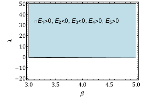
  Figure 1: The stability of the point $P_{1}$ in the parameter space of $(\beta,\lambda)$ for $(\alpha_{1}=1,s=0.1,\delta=2,\gamma=1)$.

• Point $P_{2}$: The co-ordinates of the point are $\bigg{(}x=\frac{3\sqrt{3}(\beta-1)\gamma+\sqrt{\gamma^{2}\left(27\beta^{2}-54\beta+2\delta^{2}\left(4s^{2}-9\right)+27\right)}}{\sqrt{2}\gamma\delta(2s+3)},y=0,z=-\frac{3\left(9\beta\gamma-9\gamma+\sqrt{3}\sqrt{\gamma^{2}\left(27\beta^{2}-54\beta+2\delta^{2}\left(4s^{2}-9\right)+27\right)}\right)}{\alpha_{1}\gamma\delta^{2}(2s+3)^{2}},\chi=\frac{9\beta\gamma-9\gamma+\sqrt{3}\sqrt{\gamma^{2}\left(27\beta^{2}-54\beta+2\delta^{2}\left(4s^{2}-9\right)+27\right)}}{3\delta^{2}(2s+3)},\xi=-\frac{\sqrt{3}\sqrt{\gamma^{2}\left(27\beta^{2}-54\beta+2\delta^{2}\left(4s^{2}-9\right)+27\right)}+6(\beta-1)\gamma s}{6\left(3\beta^{2}-6\beta-2\delta^{2}+3\right)}\bigg{)}$. Similar to the aforementioned point, the potential variable $y$ vanishes at this point and the effective EoS takes the same form $\omega_{\rm eff}=\frac{-3+2s}{3+2s}$. Following the same argument as above i.e., ensuring $\xi$ and $\chi$ are positive, the point becomes viable under the following conditions. Assuming the entropy $s=0.1$, the conditions are satisfied for $\gamma>0$ and $0.815\sqrt{\delta^{2}}+1\leq\beta<0.816\sqrt{\delta^{2}}+1$. This imposes a stringent constraint on $\beta$ for positive $\gamma$. Similarly, for $\gamma<0$, $1-0.816\sqrt{\delta^{2}}<\beta\leq 1-0.815\sqrt{\delta^{2}}$. For $\delta\neq 0$ and $\lambda\neq 0$, the point always becomes a saddle point.

• Point $P_{3}$: The co-ordinates of the point are $\bigg{(}x=-\frac{2\sqrt{6}s}{3\lambda+2\lambda s},y=\frac{\sqrt{9\delta\lambda^{2}-4\delta\left(\lambda^{2}-6\right)s^{2}+36(\beta-1)\lambda s}}{\sqrt{\lambda^{2}(2s+3)^{2}((\beta-1)\lambda+\delta)}},z=\frac{(2s-3)\left(3\lambda^{2}+2\left(\lambda^{2}-6\right)s\right)}{\alpha_{1}\lambda(2s+3)^{2}((\beta-1)\lambda+\delta)},\chi=-\frac{\gamma(2s-3)\left(3\lambda^{2}+2\left(\lambda^{2}-6\right)s\right)}{9\lambda(2s+3)((\beta-1)\lambda+\delta)},\xi=\frac{\gamma\lambda\left(9-4s^{2}\right)}{6(3(\beta-1)\lambda+2(\beta-1)\lambda s+4\delta s)}\bigg{)}$. At this point, both the kinetic and potential variables of the field are finite, and the effective equation of state becomes $\omega_{\rm eff}=\frac{2s-3}{2s+3}$. To discuss the existence of the point, we initially fix some values of the model parameters, considering $\beta=1$. The point exists if $\lambda>2\sqrt{3}\sqrt{\frac{s}{2s+3}},\delta>0,\gamma>0$, and the corresponding stability has been determined for $s=0.01$ in Fig.[LABEL:fig:stability_p3_beta1]. In the parameter space of $(\delta,\gamma)$, the point becomes stable for any choice of $\gamma\neq 0$. We also examine the existence and stability for other values of $\beta$, particularly $s=0.1,\beta=2$. We find that the thermodynamic constraints Eq. (55) are satisfied when $\gamma>0$, $\delta\geq 4.98,\lambda>0.61,\lambda<-\delta$, or for $\gamma>0$, $\delta\leq 4.98,\lambda<-0.61,\lambda>-\delta$. If $\gamma<0$, then $\delta>4.98$, $-0.13\delta<\lambda<-0.61$, or $\delta<-4.98,0.61<\lambda<-0.13\delta$. Hence, with these inputs, if we select the model parameters $\gamma>0,\beta=2,s=0.1$, we determine that the critical point can only be a stable fixed point when $\delta\geq 5,\lambda>2\delta+3$. It’s worth noting that the value of $\alpha_{1}$ does not affect the dynamics in any way, since it can always be absorbed in $z$. Similarly, for $\beta=3,s=0.01$, the thermodynamic parameters become positive if $\gamma>0,\lambda>0.19,\delta>-2\lambda$. The stability corresponding to this range of parameters is shown in Fig.[LABEL:fig:stability_p3_beta3].

  

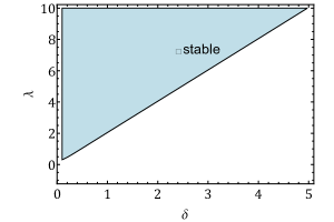
  (a)

  

  (b)

  Figure 2: The stability of the point $P_{3}$ (a) for $\beta=1,s=0.01,\alpha_{1}=1,\gamma=1$, (b) for $\beta=3,s=0.01,\alpha_{1}=1,\gamma=1$.

As we have seen, the system yields some non-trivial critical points for $s\neq 0$, and among them, one critical point is both accelerating and stable, depending on the choice of model parameters. Due to this characteristic, the point signifies the late-time phase of the universe. Having determined the ranges of model parameters that produce viable stable critical points, we will now evaluate the dynamics of the entire system considering the autonomous equations Eq. (57)–Eq. (62), which will depict the different phases of the universe. As discussed earlier, taking the equation in $s^{\prime}$ yields critical points when either $s=0$ or $z=0$. As the system is non-minimally coupled with the fluid, one expects that during the matter and future epoch, the variable $z$ must be non-vanishing. Hence, $s=0$ serves as the viable co-ordinate of the critical points. The critical points corresponding to $s=0$ and the corresponding nature of the fixed points are tabulated in Tabs.[1, 2]. The critical points are given similar nomenclature as the aforementioned fixed points.

s=0
Points	$x$	$y$	$z$	$\chi$	$\xi$
$P_{1\pm}$	$\frac{\pm p+\sqrt{6}\beta-\sqrt{6}}{2\delta}$	0	$\frac{\mp r-3\beta+3}{\text{$\alpha$1}\delta^{2}}$	$\pm\frac{\gamma\left(r+3\beta-3\right)}{3\delta^{2}}$	0
$P_{2\mp}$	$\frac{\mp r+3\beta-3}{\sqrt{6}\delta}$	0	$\frac{\pm r-3\beta+3}{\alpha_{1}\delta^{2}}$	$\mp\frac{\gamma\left(r-3\beta+3\right)}{3\delta^{2}}$	Any
$P_{3}$	0	$\frac{\sqrt{\delta}}{\sqrt{(\beta-1)\lambda+\delta}}$	$-\frac{\lambda}{\alpha_{1}((\beta-1)\lambda+\delta)}$	$\frac{\gamma\lambda}{3((\beta-1)\lambda+\delta)}$	Any
$P_{4\mp}$	$\mp 1$	0	0	0	0
$P_{5}$	$\frac{\sqrt{\frac{3}{2}}(\beta-1)}{\delta}$	$\frac{\sqrt{\frac{\left(-3\beta^{2}+6\beta+2\delta^{2}-3\right)((\beta-1)\lambda+\delta)}{\delta}}}{\sqrt{2}\sqrt{\delta((\beta-1)\lambda+\delta)}}$	$\frac{-3\beta-\delta\lambda+3}{\text{$\alpha$1}\delta^{2}}$	$\frac{2\gamma(3\beta+\delta\lambda-3)}{3\delta((\beta-1)\lambda+2\delta)}$	0

Table 1: The critical points corresponding to autonomous system of equations Eq. (57)–Eq. (62).

s=0
Points	$\omega_{\rm eff}$	$(\chi,\xi>0)$	Stability
$P_{1\pm}$	$-1$	$\gamma>0,\beta\geq\sqrt{\frac{2}{3}}\sqrt{\delta^{2}}+1$, $\gamma<0,\beta\leq 1-\sqrt{\frac{2}{3}}\sqrt{\delta^{2}}$	Indeterminate
$P_{2\mp}$	$-1$	$\gamma>0,\beta\geq\sqrt{\frac{2}{3}}\sqrt{\delta^{2}}+1$, $\gamma<0,\beta\leq 1-\sqrt{\frac{2}{3}}\sqrt{\delta^{2}}$	Saddle
$P_{3}$	$-1$	$\gamma>0,\beta\lambda+\delta>\lambda,\lambda>0,\delta>0$	see Figs.[LABEL:fig:stability_p3_beta1, LABEL:fig:stability_p3_beta3]
$P_{4\mp}$	$\mp 1$	Any	Unstable
$P_{5}$	$-\frac{\beta\lambda+\delta-\lambda}{\delta}$	$\beta\geq 1,\lambda>0,\delta>0,\gamma>0$	Indeterminate

Table 2: The condition of existence of the fixed points and their nature.

The critical points $P_{1\pm}$ produce an accelerating solution; however, when $\xi$ becomes zero, it leads to the temperature of the fluid reaching absolute zero, which is not physically viable. Moreover, the indeterminacy of the Jacobian further complicates the assessment of stability for this point. As observed in the case when $s\neq 0$, the point cannot exhibit a stable solution. Therefore, this point cannot be considered to describe the late-time era of the universe.

The critical points $P_{2\mp}$ also exhibit accelerating solutions, and $\xi$ can take any positive value. However, considering the existence range given in Tab.[2], for any values of $\beta$, the point becomes a saddle point. Thus, these points are also not considered viable descriptions for the late-time epoch of the universe.

The critical point $P_{3}$ can exhibit an accelerating solution where the field’s kinetic part vanishes, and the corresponding stability for $s\rightarrow 0$ shows similar behavior as discussed previously in Figs.[LABEL:fig:stability_p3_beta1, LABEL:fig:stability_p3_beta3]. We have also noted that for $s=0$, one of the eigenvalues becomes zero, rendering the standard linearization technique inapplicable for determining the stability of the point. However, we can employ a simple numerical trick to determine the stability even without resorting to the center manifold theorem. Since the system is non-adiabatically coupled, at any instant of time, the entropy of the dark matter fluid must be positive or zero. Hence, we numerically evolved the system by choosing initial conditions near zero, i.e., $s>0$, and observed that the system stabilizes at $P_{3}$ with $s=0$ in the far future, as demonstrated in Fig.[LABEL:fig:coord_p3_beta3]. Consequently, this point is a physically viable fixed point for describing the late-time phase of the universe.

The other critical points $P_{4\mp}$ rely solely on the field’s kinetic component, while the co-ordinate $z$ vanishes. This leads to the autonomous equation in $s^{\prime}$ becoming zero, i.e., $s^{\prime}=0$, without requiring $s=0$. Consequently, the variable $s$ can take any value. The effective equation of state at this point is $1$, indicating a stiff matter solution, which reflects the minimally coupled behavior of quintessence in the far past epoch. Since $s$ can take any value, this suggests that during the past epoch, the system was non-adiabatically coupled.

At critical point $P_{5}$, all the field components are finite, but the parameter corresponding to the temperature vanishes. For $\beta=1$, the effective equation of state becomes $-1$. If $\beta>1$, then $0<\lambda<-\frac{\delta}{2\beta-2}$. However, since $\xi$ vanishes for any choice of model parameters and the Jacobian becomes indeterminate, as discussed earlier, this point cannot be considered physically relevant.

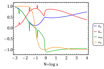
(a)

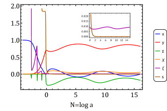
(b)

Figure 3: The numerical evolution of cosmological parameters for $(\gamma=1,\beta=3,\alpha_{1}=1,\delta=2,\lambda=0.5)$ with the initial conditions $x(0)=0.02,y(0)=0.7,z(0)=-0.3,\chi(0)=0.03,\xi(0)=0.009,s(0)=0.15$.

After carefully studying the nature of critical points for $s\neq 0$ and $s=0$, we can conclude that the physically viable critical point that describes the behavior of the late-time epoch of the universe is $P_{3}$. Therefore, to analyze the system’s overall dynamics, we numerically simulate the autonomous equations Eq. (57)–Eq. (62), by selecting the benchmark points $\beta=3$, $\delta=2$, $\lambda=0.5$, $\alpha_{1}=1$. Corresponding to these benchmark points, the coordinates of the point $P_{3}$ become: $(x=0,y=0.82,z=-0.17,\chi=0.06,\xi=\xi)$, and the corresponding field and fluid fractional densities become $\Omega_{\phi}=0.67$, $\Omega_{M}=0.5$. The numerical evolution of the cosmological parameters has been demonstrated in Fig.[LABEL:fig:evo_p3_beta3] against $N=\ln a$, ranging from the past epoch to the future epoch of the universe.

At the very past epoch of the universe, the field’s kinetic component dominates, showing the behavior described by points $P_{4\mp}$. At this epoch, the effective equation of state and the field’s equation of state $\omega_{\phi}\equiv\frac{x^{2}-y^{2}}{x^{2}+y^{2}}$ both become $1$. As the universe enters the matter-dominated phase, the effective equation of state becomes zero, and it continuously increases towards negative values. However, a steeper fall can be observed in the behavior of $\omega_{\phi}$. Unlike the standard model of cosmology ($\Lambda$CDM) or other versions of minimally coupled quintessence field with dark matter fluid, as the system enters the current epoch ($a=1$ or $N=0$), the dark energy dominates over the fluid component and the effective equation of state becomes $-1$. However, in the current scenario, the fluid energy density dominates over the field density, forcing the effective equation of state to cross the phantom barrier ($-1$) for a brief period of time. This is the consequence of non-adiabatic energy transfer occurring between the field and the fluid.

As the system further evolves into the future epoch, the model stabilizes to $\omega_{\rm eff}=-1$ with a dominating field energy density. However, because of the interaction, the fluid energy density does not get diluted. At any instant of time, the fluid and field energy densities can take values greater than $1$, however, the total energy density of the system $\Omega_{\rm tot}=\Omega_{M}+\Omega_{\phi}+\alpha_{1}z$ always remains $1$ as shown by the gray dashed line parallel to the $x$-axis. One way to interpret this behavior is as discussed in ref.[64], where it is noted that it’s nearly impossible to distinguish between dark sectors and gravity; therefore, they are degenerate. Alongside the cosmological parameters, we have also shown the evolution of dynamical variables in Fig.[LABEL:fig:coord_p3_beta3], and found that the thermodynamic variables throughout the evolution follows the constraint Eq. (55).

In addition to stability, we have also assessed the viability of the model by comparing it with the $\Lambda$CDM model using available observational data from Hubble $(43)$ and Pantheon+ $(1701)$ (url) datasets [65, 66]. Utilizing the relation between the scale factor $a$ and redshift $\tilde{z}$, $a=1/(1+\tilde{z})$, we can derive the evolution of the Hubble parameter as follows:

$$\frac{dH}{d\tilde{z}}=\frac{3}{2}\frac{1}{(1+\tilde{z})}H(\tilde{z})(1+\omega_{\rm eff}).$$ (63)

The Hubble parameter has been fitted with observational Hubble dataset (OHD) alongside the $\Lambda$CDM model, using dark matter density $\Omega_{m}=0.25$, cosmological constant fractional density $\Omega_{\Lambda}=0.75$, and $H_{0}=67$ (in units of km/s/Mpc), as shown in Fig.[LABEL:fig:hubble_beta3]. The current model has been simulated using the same benchmark point and initial conditions as shown in Fig.[LABEL:fig:evo_p3_beta3], with $H_{0}=66$, to better match observations. The non-linear evolution of $H(\tilde{z})$ near $\tilde{z}\rightarrow 0,1.5$ shows a significant deviation from the standard model. By testing the model with larger datasets using sampling techniques like MCMC, it may contribute to lowering the discrepancy in the Hubble value.

To fit the model with the Pantheon+ data, we utilize the distance modulus $\mu$ relation with redshift,

$$\mu=5\log_{10}(d_{L})+25,$$ (64)

where the luminosity distance is given by,

$$d_{L}=2.99\times 10^{5}(1+\tilde{z})\int_{0}^{\tilde{z}}\frac{1}{H(\tilde{z})}d\tilde{z}\ ,$$ (65)

The evolution of $\mu$ for the $\Lambda$CDM model overlaps with the current model, as shown in Fig.[LABEL:fig:supernova_dist_1]. It’s noteworthy that we have selected the model parameter $\beta=3$ because the evolution of the Hubble parameter closely resembles that of $\Lambda$CDM for this case.

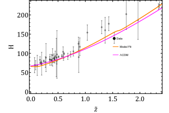
(a)

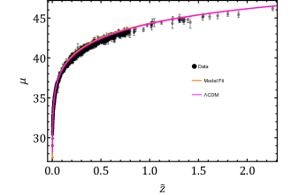
(b)

Figure 4: (a) The Hubble evolution and (b) the distance modulus corresponding to $\Lambda$CDM is evaluated with $\Omega_{M}=0.25,\Omega_{\Lambda}=0.75,H(0)=67.0$. The current model has been fitted for $(\gamma=1,\beta=3,\alpha_{1}=1,\delta=2,\lambda=0.5)$ with the initial conditions $x(0)=0.02,y(0)=0.7,z(0)=-0.3,\chi(0)=0.03,\xi(0)=0.009,s(0)=0.15,H(0)=66.0$.

VI Conclusion

The study delves into a non-minimal coupling scenario between the quintessence field and a pressureless fluid, examined thoroughly through the variational principle. By incorporating one of the Lagrange parameters $\varphi$ into the interacting Lagrangian, we altered the conservation laws governing the fluid’s number density and entropy density. Consequently, the fluid sector introduces an additional pressure termed creation pressure. Upon evaluating the covariant derivative of the energy-momentum tensor, it becomes apparent that individual components are no longer conserved, facilitating the flow of energy from the field to the fluid through the field derivative of the interaction function $f_{,\phi}\dot{\phi}$.

We assessed the background stability of the model by considering an exponential type of interaction. The system yielded a stable critical point capable of producing an accelerating solution in the far future epoch of the universe, dominated by the scalar field energy density with a finite fluid energy density. Furthermore, numerical simulations corresponding to the interaction $f\propto\rho^{3}$ revealed that during the current epoch, the fluid density predominates, resulting in a phantom equation of state for a brief period.

To evaluate the viability of the model, we conducted simulations with the Hubble and Pantheon+ data sets alongside the $\Lambda$CDM model. The model demonstrates the ability to mimic $\Lambda$CDM behavior while simultaneously exhibiting deviations. In future work, we intend to conduct a comprehensive statistical analysis to further assess the model’s viability with various data sets.

References

References

- Perlmutter et al. [1999] S. Perlmutter et al. (Supernova Cosmology Project), Measurements of and from 42 high redshift supernovae, Astrophys. J. 517, 565 (1999), arXiv:astro-ph/9812133 .
- Riess et al. [1998] A. G. Riess et al. (Supernova Search Team), Observational evidence from supernovae for an accelerating universe and a cosmological constant, Astron. J. 116, 1009 (1998), arXiv:astro-ph/9805201 .
- Spergel et al. [2003] D. N. Spergel et al. (WMAP), First year Wilkinson Microwave Anisotropy Probe (WMAP) observations: Determination of cosmological parameters, Astrophys. J. Suppl. 148, 175 (2003), arXiv:astro-ph/0302209 .
- Sherwin et al. [2011] B. D. Sherwin et al., Evidence for dark energy from the cosmic microwave background alone using the Atacama Cosmology Telescope lensing measurements, Phys. Rev. Lett. 107, 021302 (2011), arXiv:1105.0419 [astro-ph.CO] .
- Wright [2007] E. L. Wright, Constraints on Dark Energy from Supernovae, Gamma Ray Bursts, Acoustic Oscillations, Nucleosynthesis and Large Scale Structure and the Hubble constant, Astrophys. J. 664, 633 (2007), arXiv:astro-ph/0701584 .
- Kwan et al. [2017] J. Kwan et al. (DES), Cosmology from large-scale galaxy clustering and galaxy–galaxy lensing with Dark Energy Survey Science Verification data, Mon. Not. Roy. Astron. Soc. 464, 4045 (2017), arXiv:1604.07871 [astro-ph.CO] .
- Abbott et al. [2022] T. M. C. Abbott et al. (DES), Dark Energy Survey Year 3 results: A 2.7% measurement of baryon acoustic oscillation distance scale at redshift 0.835, Phys. Rev. D 105, 043512 (2022), arXiv:2107.04646 [astro-ph.CO] .
- Scolnic et al. [2022] D. Scolnic et al., The Pantheon+ Analysis: The Full Data Set and Light-curve Release, Astrophys. J. 938, 113 (2022), arXiv:2112.03863 [astro-ph.CO] .
- Aghanim et al. [2020] N. Aghanim et al. (Planck), Planck 2018 results. VI. Cosmological parameters, Astron. Astrophys. 641, A6 (2020), [Erratum: Astron.Astrophys. 652, C4 (2021)], arXiv:1807.06209 [astro-ph.CO] .
- Copeland et al. [2006] E. J. Copeland, M. Sami, and S. Tsujikawa, Dynamics of dark energy, Int. J. Mod. Phys. D 15, 1753 (2006), arXiv:hep-th/0603057 .
- Weinberg [1989] S. Weinberg, The Cosmological Constant Problem, Rev. Mod. Phys. 61, 1 (1989).
- Rugh and Zinkernagel [2002] S. E. Rugh and H. Zinkernagel, The Quantum vacuum and the cosmological constant problem, Stud. Hist. Phil. Sci. B 33, 663 (2002), arXiv:hep-th/0012253 .
- Padmanabhan [2003] T. Padmanabhan, Cosmological constant: The Weight of the vacuum, Phys. Rept. 380, 235 (2003), arXiv:hep-th/0212290 .
- Carroll et al. [1992] S. M. Carroll, W. H. Press, and E. L. Turner, The Cosmological constant, Ann. Rev. Astron. Astrophys. 30, 499 (1992).
- Arkani-Hamed et al. [2000] N. Arkani-Hamed, L. J. Hall, C. F. Kolda, and H. Murayama, A New perspective on cosmic coincidence problems, Phys. Rev. Lett. 85, 4434 (2000), arXiv:astro-ph/0005111 .
- Velten et al. [2014] H. E. S. Velten, R. F. vom Marttens, and W. Zimdahl, Aspects of the cosmological “coincidence problem”, Eur. Phys. J. C 74, 3160 (2014), arXiv:1410.2509 [astro-ph.CO] .
- Sotiriou and Faraoni [2010] T. P. Sotiriou and V. Faraoni, f(R) Theories Of Gravity, Rev. Mod. Phys. 82, 451 (2010), arXiv:0805.1726 [gr-qc] .
- Nojiri and Odintsov [2006] S. Nojiri and S. D. Odintsov, Introduction to modified gravity and gravitational alternative for dark energy, eConf C0602061, 06 (2006), arXiv:hep-th/0601213 .
- Beltrán Jiménez et al. [2018] J. Beltrán Jiménez, L. Heisenberg, and T. Koivisto, Coincident General Relativity, Phys. Rev. D 98, 044048 (2018), arXiv:1710.03116 [gr-qc] .
- Cai et al. [2016] Y.-F. Cai, S. Capozziello, M. De Laurentis, and E. N. Saridakis, f(T) teleparallel gravity and cosmology, Rept. Prog. Phys. 79, 106901 (2016), arXiv:1511.07586 [gr-qc] .
- Peebles and Ratra [2003] P. J. E. Peebles and B. Ratra, The Cosmological Constant and Dark Energy, Rev. Mod. Phys. 75, 559 (2003), arXiv:astro-ph/0207347 .
- Nishioka and Fujii [1992] T. Nishioka and Y. Fujii, Inflation and the decaying cosmological constant, Phys. Rev. D 45, 2140 (1992).
- Armendariz-Picon et al. [2000] C. Armendariz-Picon, V. F. Mukhanov, and P. J. Steinhardt, A Dynamical solution to the problem of a small cosmological constant and late time cosmic acceleration, Phys. Rev. Lett. 85, 4438 (2000), arXiv:astro-ph/0004134 .
- Armendariz-Picon et al. [2001] C. Armendariz-Picon, V. F. Mukhanov, and P. J. Steinhardt, Essentials of k essence, Phys. Rev. D 63, 103510 (2001), arXiv:astro-ph/0006373 .
- Chiba et al. [2000] T. Chiba, T. Okabe, and M. Yamaguchi, Kinetically driven quintessence, Phys. Rev. D 62, 023511 (2000), arXiv:astro-ph/9912463 .
- Kamenshchik et al. [2001] A. Y. Kamenshchik, U. Moschella, and V. Pasquier, An Alternative to quintessence, Phys. Lett. B 511, 265 (2001), arXiv:gr-qc/0103004 .
- Bento et al. [2002] M. C. Bento, O. Bertolami, and A. A. Sen, Generalized Chaplygin gas, accelerated expansion and dark energy matter unification, Phys. Rev. D 66, 043507 (2002), arXiv:gr-qc/0202064 .
- Ellis et al. [1989] J. R. Ellis, S. Kalara, K. A. Olive, and C. Wetterich, Density Dependent Couplings and Astrophysical Bounds on Light Scalar Particles, Phys. Lett. B 228, 264 (1989).
- Amendola [1999] L. Amendola, Scaling solutions in general nonminimal coupling theories, Phys. Rev. D 60, 043501 (1999), arXiv:astro-ph/9904120 .
- Farrar and Peebles [2004] G. R. Farrar and P. J. E. Peebles, Interacting dark matter and dark energy, Astrophys. J. 604, 1 (2004), arXiv:astro-ph/0307316 .
- Zimdahl and Pavon [2004] W. Zimdahl and D. Pavon, Statefinder parameters for interacting dark energy, Gen. Rel. Grav. 36, 1483 (2004), arXiv:gr-qc/0311067 .
- Sadjadi and Alimohammadi [2006] H. M. Sadjadi and M. Alimohammadi, Cosmological coincidence problem in interactive dark energy models, Phys. Rev. D 74, 103007 (2006), arXiv:gr-qc/0610080 .
- Hussain et al. [2023a] S. Hussain, S. Chakraborty, N. Roy, and K. Bhattacharya, Dynamical systems analysis of tachyon-dark-energy models from a new perspective, Phys. Rev. D 107, 063515 (2023a), arXiv:2208.10352 [gr-qc] .
- Das et al. [2023] S. Das, S. Hussain, D. Nandi, R. O. Ramos, and R. Silva, Stability analysis of warm quintessential dark energy model, Phys. Rev. D 108, 083517 (2023), arXiv:2306.09369 [gr-qc] .
- Sen and Sen [2001] S. Sen and A. A. Sen, Late time acceleration in Brans-Dicke cosmology, Phys. Rev. D 63, 124006 (2001), arXiv:gr-qc/0010092 .
- Bertolami et al. [2008] O. Bertolami, F. S. N. Lobo, and J. Paramos, Non-minimum coupling of perfect fluids to curvature, Phys. Rev. D 78, 064036 (2008), arXiv:0806.4434 [gr-qc] .
- Bertolami and Martins [2012] O. Bertolami and A. Martins, On the dynamics of perfect fluids in non-minimally coupled gravity, Phys. Rev. D 85, 024012 (2012), arXiv:1110.2379 [gr-qc] .
- Tsujikawa and Sami [2007] S. Tsujikawa and M. Sami, String-inspired cosmology: Late time transition from scaling matter era to dark energy universe caused by a Gauss-Bonnet coupling, JCAP 01, 006, arXiv:hep-th/0608178 .
- Bettoni and Liberati [2015] D. Bettoni and S. Liberati, Dynamics of non-minimally coupled perfect fluids, JCAP 08, 023, arXiv:1502.06613 [gr-qc] .
- Boehmer et al. [2015a] C. G. Boehmer, N. Tamanini, and M. Wright, Interacting quintessence from a variational approach Part I: algebraic couplings, Phys. Rev. D 91, 123002 (2015a), arXiv:1501.06540 [gr-qc] .
- Boehmer et al. [2015b] C. G. Boehmer, N. Tamanini, and M. Wright, Interacting quintessence from a variational approach Part II: derivative couplings, Phys. Rev. D 91, 123003 (2015b), arXiv:1502.04030 [gr-qc] .
- Chatterjee et al. [2021] A. Chatterjee, S. Hussain, and K. Bhattacharya, Dynamical stability of the k-essence field interacting nonminimally with a perfect fluid, Phys. Rev. D 104, 103505 (2021), arXiv:2105.00361 [gr-qc] .
- Bhattacharya et al. [2023] K. Bhattacharya, A. Chatterjee, and S. Hussain, Dynamical stability in presence of non-minimal derivative dependent coupling of k-essence field with a relativistic fluid, Eur. Phys. J. C 83, 488 (2023), arXiv:2206.12398 [gr-qc] .
- Koivisto et al. [2015] T. S. Koivisto, E. N. Saridakis, and N. Tamanini, Scalar-Fluid theories: cosmological perturbations and large-scale structure, JCAP 09, 047, arXiv:1505.07556 [astro-ph.CO] .
- Kase and Tsujikawa [2020] R. Kase and S. Tsujikawa, Scalar-Field Dark Energy Nonminimally and Kinetically Coupled to Dark Matter, Phys. Rev. D 101, 063511 (2020), arXiv:1910.02699 [gr-qc] .
- Hussain et al. [2023b] S. Hussain, A. Chatterjee, and K. Bhattacharya, Dynamical stability in models where dark matter and dark energy are nonminimally coupled to curvature, Phys. Rev. D 108, 103502 (2023b), arXiv:2305.19062 [gr-qc] .
- Shaily et al. [2024] Shaily, A. Singh, J. K. Singh, and S. Hussain, Stability analysis of a dark energy model in Rastall gravity, (2024), arXiv:2402.08709 [gr-qc] .
- Tamanini [2015] N. Tamanini, Phenomenological models of dark energy interacting with dark matter, Phys. Rev. D 92, 043524 (2015), arXiv:1504.07397 [gr-qc] .
- Brown [1993] J. D. Brown, Action functionals for relativistic perfect fluids, Class. Quant. Grav. 10, 1579 (1993), arXiv:gr-qc/9304026 .
- Di Valentino et al. [2021] E. Di Valentino, O. Mena, S. Pan, L. Visinelli, W. Yang, A. Melchiorri, D. F. Mota, A. G. Riess, and J. Silk, In the realm of the Hubble tension—a review of solutions, Class. Quant. Grav. 38, 153001 (2021), arXiv:2103.01183 [astro-ph.CO] .
- Krishnan et al. [2020] C. Krishnan, E. O. Colgáin, Ruchika, A. A. Sen, M. M. Sheikh-Jabbari, and T. Yang, Is there an early Universe solution to Hubble tension?, Phys. Rev. D 102, 103525 (2020), arXiv:2002.06044 [astro-ph.CO] .
- Davis et al. [2019] T. M. Davis, S. R. Hinton, C. Howlett, and J. Calcino, Can redshift errors bias measurements of the Hubble Constant?, Mon. Not. Roy. Astron. Soc. 490, 2948 (2019), arXiv:1907.12639 [astro-ph.CO] .
- Ford [1987] L. H. Ford, Gravitational Particle Creation and Inflation, Phys. Rev. D 35, 2955 (1987).
- Prigogine et al. [1988] I. Prigogine, J. Geheniau, E. Gunzig, and P. Nardone, Thermodynamics of cosmological matter creation, Proc. Nat. Acad. Sci. 85, 7428 (1988).
- Lima et al. [2012] J. A. S. Lima, S. Basilakos, and F. E. M. Costa, New Cosmic Accelerating Scenario without Dark Energy, Phys. Rev. D 86, 103534 (2012), arXiv:1205.0868 [astro-ph.CO] .
- Zimdahl [1996] W. Zimdahl, Bulk viscous cosmology, Phys. Rev. D 53, 5483 (1996), arXiv:astro-ph/9601189 .
- Nunes and Pan [2016] R. C. Nunes and S. Pan, Cosmological consequences of an adiabatic matter creation process, Mon. Not. Roy. Astron. Soc. 459, 673 (2016), arXiv:1603.02573 [gr-qc] .
- Bhattacharya et al. [2022] K. Bhattacharya, A. Chatterjee, and S. Hussain, The nature of cosmological metric perturbations in presence of gravitational particle production, Gen. Rel. Grav. 54, 84 (2022), arXiv:2007.00904 [gr-qc] .
- Rendall [2002] A. D. Rendall, Cosmological models and center manifold theory, Gen. Rel. Grav. 34, 1277 (2002), arXiv:gr-qc/0112040 .
- Bahamonde et al. [2018] S. Bahamonde, C. G. Böhmer, S. Carloni, E. J. Copeland, W. Fang, and N. Tamanini, Dynamical systems applied to cosmology: dark energy and modified gravity, Phys. Rept. 775-777, 1 (2018), arXiv:1712.03107 [gr-qc] .
- Dutta et al. [2018] J. Dutta, W. Khyllep, and N. Tamanini, Dark energy with a gradient coupling to the dark matter fluid: cosmological dynamics and structure formation, JCAP 01, 038, arXiv:1707.09246 [gr-qc] .
- Coley [2003] A. A. Coley, Dynamical systems and cosmology (Kluwer, Dordrecht, Netherlands, 2003).
- Ivanov and Prodanov [2019] R. I. Ivanov and E. M. Prodanov, On the Cosmological Models with Matter Creation, Eur. Phys. J. C 79, 973 (2019), arXiv:1911.04380 [gr-qc] .
- Kunz [2009] M. Kunz, The dark degeneracy: On the number and nature of dark components, Phys. Rev. D 80, 123001 (2009), arXiv:astro-ph/0702615 .
- Cao et al. [2021] S. Cao, T.-J. Zhang, X. Wang, and T. Zhang, Cosmological Constraints on the Coupling Model from Observational Hubble Parameter and Baryon Acoustic Oscillation Measurements, Universe 7, 57 (2021), arXiv:2103.03670 [astro-ph.CO] .
- Perivolaropoulos and Skara [2023] L. Perivolaropoulos and F. Skara, On the homogeneity of SnIa absolute magnitude in the Pantheon+ sample, Mon. Not. Roy. Astron. Soc. 520, 5110 (2023), arXiv:2301.01024 [astro-ph.CO] .