Irrational random utility models^∗

Abstract.

We show that the set of aggregate choices of a population of rational decision-makers - random utility models (RUMs) - can be represented by a population of irrational ones if, and only if, their preferences are sufficiently uncorrelated. We call this representation: Irrational RUM. We then show that almost all RUMs can be represented by a population in which at least some decision-makers are irrational and that under specific conditions their irrational behavior is unconstrained.

Keywords: Stochastic choice, random utility models, rationality.

JEL Classification: D00, D90, D91.

1. Introduction

The random utility model (RUM) is the most renowned model of stochastic choice and it is the leading notion of stochastic rationality in economics (McFadden & Richter (1990), McFadden (2006)): choice probabilities satisfy the RUM hypothesis if they result from the aggregation of the choices of rational - preference maximizing - decision-makers. These aggregate choices are normally referred to as stochastically rational.

A starting point of the present paper is the observation that aggregate choices may be stochastically rational even if all decision-makers are irrational, i.e. they violate the tenets of rationality. The intuition behind this observation is simple. If the irrationalities of decision-makers are sufficiently uncorrelated, they will cancel out, and aggregate data will appear as if stochastically rational. We call the subset of RUMs that display this property ”irrational” [I-RUM].

Our first main result is a characterization of I-RUMs using bounds on the ”correlation” between the preferences of the rational decision-makers that may represent the RUM. We build on the intuition above and show that a population of rational decision-makers is also represented by a population of irrational ones whenever their preferences are sufficiently uncorrelated. Our second main result focuses on the RUMs that can be represented by a population in which at least some decision-makers are irrational, we call them ”partially irrational” [pI-RUM]. We show that almost all RUMs are partially irrational, and in fact, that all RUMs with full support (e.g. Logit model) are. In a nutshell, considering irrational decision-makers can have severe consequences for the interpretation of stochastically rational data, in fact, so severe as to undermine the very (rational) essence of the RUM hypothesis.

A relevant implication of our results relates to the falsifiability of the rational interpretation of the RUM hypothesis; i.e. even if rationality is violated by all decision-makers the RUM hypothesis may fail to be rejected. In the second part of the paper, we discuss this interpretation in more detail by focusing on some properties of pi-RUMs. First, we show that, under the RUM hypothesis, there is always a fraction of decision-makers whose behavior is unconstrained, i.e. for this fraction of decision-makers rationality can be violated in the most extreme sense (while aggregate data is still consistent with RUM). This result is deliberately demanding from an irrationality perspective implying that such a fraction of irrational decision-makers may be small. We, therefore, go on to show that the fraction of irrational decision-makers that are compatible with the RUM hypothesis is larger the less constrained is the set of possible irrational behaviors. These results have important consequences for empirical applications where irrational behavior is unlikely to be extreme (i.e. more constrained) implying that the issue of the non-falsifiability is likely to be widespread.

We illustrate our main results and intuitions through one simple example.

Example 1 (Irrational RUMs).

An analyst observes the aggregate choice probabilities in all non-empty menus of a set of three alternatives - ”chicken” ($c$), ”steak” ($s$), and ”frogs’ legs” ($f$) - from a population where 1/2 of the decision-makers have preference $c\hskip 1.49994ptP_{1}\hskip 1.49994pts\hskip 1.49994ptP_{1}\hskip 1.49994ptf$ and 1/2 have preference $s\hskip 1.49994ptP_{2}\hskip 1.49994ptc\hskip 1.49994ptP_{2}\hskip 1.49994ptf$. The first and second column in the table below displays the choices of these rational decision-makers from each menu with $P_{1}$’s choices highlighted in red and $P_{2}$’s in blue.

Menu	${\color[rgb]{0,0,0}\max(A,P_{1})}$	$\max(A,P_{2})$	$c_{1}(A)$	$c_{2}(A)$
$csf$	${\color[rgb]{1,0,0}c}$	${\color[rgb]{0,0,1}s}$	${\color[rgb]{0,0,1}s}$	${\color[rgb]{1,0,0}c}$
$cs$	${\color[rgb]{1,0,0}c}$	${\color[rgb]{0,0,1}s}$	${\color[rgb]{1,0,0}c}$	${\color[rgb]{0,0,1}s}$
$cf$	${\color[rgb]{1,0,0}c}$	${\color[rgb]{0,0,1}c}$	${\color[rgb]{1,0,0}c}$	${\color[rgb]{1,0,0}c}$
$sf$	${\color[rgb]{1,0,0}s}$	${\color[rgb]{0,0,1}s}$	${\color[rgb]{1,0,0}s}$	${\color[rgb]{1,0,0}s}$

We now provide a different interpretation of the aggregate data from an irrational perspective. Consider the Luce & Raiffa’s dinner example (Luce & Raiffa, 1957) in which a decision-maker chooses chicken when only steak is available, but switches to steak whenever also frogs’ legs are available even if he dislikes frogs’ legs. Imagine now another decision-maker with the same behavior but who chooses steak when only chicken is available and switches to chicken in the presence of frogs’ legs. These well-known irrational behaviors are summarized by the choices $c_{1}$ and $c_{2}$ in the table. Note that $c_{1}$ and $c_{2}$ agree with $P_{1}$ except in one menu where choices are obtained by ”switching” the choices of $P_{1}$ and $P_{2}$. A population in which 1/2 of the decision-makers choose according to $c_{1}$ and $c_{2}$ will induce the same aggregate data as the original population of rational decision-makers.

Although the RUM in the above example has an irrational representation, if the probability distribution on the preferences $P_{1}$ and $P_{2}$ is perturbed only slightly then an irrational representation no longer exists. To see this, suppose that 51% of the rational decision-makers have preference $P_{1}$ (so prefer $c$ to $s$ and $f$). Then, in an irrational representation, 51% of the irrational decision-makers must choose $c$ when $s$ is available. However, an irrational decision-maker who chooses $c$ from the menu $csf$ must either choose $s$ from $cs$ or $f$ from $cf$ (to induce a violation of rationality). Since $51\%$ of the irrational decision-makers choose $c$ from $csf$ and $f$ is never chosen in $cf$, this implies that $51\%$ of the irrational decision makers must choose $s$ when $c$ available! A contradiction. In our main theorem, we characterize the exact conditions on the aggregate data under which irrational representations exist.

Example 1 questions, at a fundamental level, the non-falsifiability of the rational interpretation of the RUM hypothesis. A population of decision-makers with a uniform distribution on $c_{1}$ and $c_{2}$ fails to reject the RUM hypothesis even though all decision-makers are irrational. However, an irrational representation exists only if the irrational behaviors (described by $c_{1}$ and $c_{2}$) are sufficiently uncorrelated. Below, we modify the opening example to show that the behaviors of irrational decision-makers can instead be unrestricted (and highly correlated) and still be aligned with the RUM hypothesis.

Example 1 (continued).

Consider a population where a fraction of decision-makers are rational and, differently from above, have a uniform distribution on the set of preferences on $\{c,s,f\}$; while the remaining ones are irrational. Simple calculations show that whenever at least 6/7 of the decision-makers are rational then the behavior of the remaining irrational ones is unconstrained w.r.t. stochastic rationality.

This bound may seem extreme at first glance, however, it assumes extreme scenarios such as those in which every irrational decision-maker makes the same mistake. To see how the bound changes with the set of potential irrational behaviors, if $c_{1}$ is at most twice as likely to appear as $c_{2}$, the fraction of irrational decision-makers compatible with the RUM hypothesis increases from 1/7 to 1/3, while, as shown before, if $c_{1}$ and $c_{2}$ are equally probable this fraction becomes one.

1.1. Related Literature

Our study of irrational behavior within the RUM contributes to a longstanding literature on stochastic choice. Most closely, our framework aligns with some recent papers that also study probability distributions on choice functions and their aggregation. Dardanoni et al. (2020) and Dardanoni et al. (2023) refer to this approach as ”mixture choice functions” while Filiz-Ozbay & Masatlioglu (2023) as ”random choice models”. In this paper, we will adopt this second nomenclature. The focus of these papers is, however, different from ours as they tackle the well-known identification issues of stochastic choice models. Dardanoni et al. (2020) provide conditions under which an analyst who only observes aggregate choice probabilities can identify cognitive parameters under specific models and restrictive assumptions (preference homogeneity or known distribution of preferences). Dardanoni et al. (2023) refine these results by assuming that the analyst observes each decision-maker’s choices and show that this allows the identification of both cognitive parameters and preferences. Filiz-Ozbay & Masatlioglu (2023), instead, study the aggregation of a population of decision-makers who are possibly boundedly rational under the assumption that the collection of their choices is progressive - a generalization to the well-known single-crossing property (Apesteguia et al., 2017). The authors show that this restriction on the set of choice functions allows the identification of the unique sources of heterogeneity in the data.

We also contribute to the longstanding literature on the characterizations of the RUM (Block & Marschak (1960), Falmagne (1978), Barberá & Pattanaik (1986), McFadden & Richter (1990), Gilboa (1990), Fiorini (2004), McFadden (2006), Stoye (2019)), and its special cases such as single-crossing RUM (Apesteguia et al., 2017), and Dual RUM (Manzini & Mariotti, 2018); as well as the study of its non-identifiability issues (Turansick (2022), Suleymanov (2023)). More specifically, our work is closely related to Manzini & Mariotti (2018) as Dual RUMs will be crucial in our characterization of both I-RUMs and pI-RUMs, and to Turansick (2022), Suleymanov (2023) as by considering irrational decision-makers our results extend further the non-identifiability issues of the RUM.

Identifiability and falsifiability under the RUM hypothesis are tightly connected issues as they both leverage the tension between aggregate and individual behavior which is an old problem within the literature on the theory of demand. It was first recognized by Becker (1962) who pointed out that the aggregation of erratic consumers may lead to a well-behaved aggregate demand function. The connection between heterogeneity and aggregate behavior was then investigated more in-depth by Grandmont (1992) who, without relying on individual rationality, provided sufficient conditions for the distribution of individual demand functions that guarantee a well-behaved aggregation. These issues have been long recognized within the literature of demand estimation that often incorporates tests of individual rationality, e.g. see Blundell et al. (2003). In this tradition, two relevant papers for us are Hoderlein & Stoye (2014), and Hoderlein & Stoye (2015). The authors ask broadly what knowledge of the ”joint distribution of demand”, i.e. individual demand functions, the analyst may have by knowing only the marginal distribution of demand, i.e. aggregate choice probabilities. Their setting is therefore similar to ours and, to the best of our knowledge, they are the first to introduce Fréchet bounds to bound the fraction of (ir)rational consumers, i.e. they prove, within the context of the theory of demand, the necessity of these bounds. Our results abstract from the framework of the theory of demand to provide necessary and sufficient conditions for stochastic rationality to coexist with individual irrationality. We believe our abstraction could lead to the application of these intuitions to broader contexts where different definitions of (ir)rationality may apply.

The view of our results from the lens of falsifiability of the rational interpretation of the RUM hypothesis is instead relatively novel. Im & Rehbeck (2022) focus on a restrictive setting of two consumption goods and two observations to show that unless more than half of the population is irrational, the population overall could be stochastically rationalizable. They refer to this notion as ”false acceptance of stochastic rationalizability”. In this paper, we generalize their observation by characterizing the exact conditions under which stochastic rationalizable choices have an irrational representation. In our final discussion section, we borrow some of their observations to show, within the framework of the theory of demand, that considering only rational representations of RUMs may lead to welfare misjudgments.

Finally, our results contribute to the literature on tests of the RUM hypothesis: Kitamura & Stoye (2018), McCausland et al. (2020), Aguiar & Kashaev (2021), Smeulders et al. (2021), Deb et al. (2023). More specifically, we discuss our results in the framework of Kitamura & Stoye (2018). The authors provide a statistical test for the RUM hypothesis based on the distance between the observed choice probabilities and the set of RUMs which implies that whenever the distance is zero, i.e. the choice probabilities are stochastically rational, the RUM hypothesis is accepted. This observation is a direct consequence of the restriction of the set of choice functions to the rational ones. In weakening this assumption, our results show that the sole focus on aggregate choice probabilities often does not provide any evidence about individual behavior and that if evidence of individual rationality exists they often do not depend on whether aggregate choice probabilities are rational or not.

The paper is organized as follows: in section 2, we introduce some preliminary notions; in section 3 we define I-RUMs, pI-RUMs, and introduce our correlation bounds; in section 4 we state and discuss our characterization theorems; in section 5, we discuss the falsifiability of the rational interpretation of RUMs; finally, in section 6, we discuss some paradoxical implications of our results. In the appendix, we first discuss some preliminary notions and auxiliary results (appendix A), then we prove our main theorem (appendix B) and, finally, we provide other proofs that are omitted from the main text (appendix C).

2. Preliminaries

We denote by $X$ a finite set of alternatives with $|X|=N$. A subset $A\subseteq X$ is called a menu. Let $\mathcal{A}$ denote the collection of all nonempty menus of $X$ with cardinality greater than two, and let $|\mathcal{A}|=K$.

The empirical primitive is a stochastic choice function, i.e. a map $\rho:X\times\mathcal{A}\to[0,1]$ such that i) $\sum_{a\in A}\rho(a,A)=1$ for all $A\in\mathcal{A}$ and ii) $\rho(a,A)=0$ for all $a\in X\setminus A$.

Our decision-makers choose once from several menus. Their choices are described by a choice function, i.e. a map $c:\mathcal{A}\to X$ such that $c(A)\in A$ for all $A\in\mathcal{A}$. We are particularly interested in choices that result from the act of preference maximization. Let $P$ be a strict linear order, henceforth ”preference”, we denote by $c_{P}$ a choice function that is rationalizable by a preference and refer to it as rational, i.e. $c_{P}(A)=\max(P,A)=\{a\in A:aPb\,\,\text{for all}\,\,b\in A\}$ for all $A\in\mathcal{A}$. If a choice function is not rationalizable we will instead refer to it as irrational. We let $\mathcal{C}$ denote the collection of all choice functions and $\mathcal{P}$ the set of rationalizable choice functions. Note that there is a one-to-one correspondence between the set of rational choice functions and the set of preferences, therefore, throughout the paper we refer to them as $c_{P}$ or $P$ interchangeably. Finally, and most importantly, we do not assume that the analyst observes the individual choice functions even if, especially in experimental settings, this is often the case.

A random choice model (RCM) is a probability distribution $\mu$ on $\mathcal{C}$. The support of $\mu$, denoted $\text{supp}(\mu)$, is the set of choice functions with strictly positive probability, i.e. $\{c\in\mathcal{C}:\mu(c)>0\}$. The RCM stochastic choice function is $\rho_{\mu}(a,A)=\mu(\mathcal{C}(a,A))$ for all $a\in A$ and $A\subseteq X$, where $\mathcal{C}(a,A)=\{c\in\mathcal{C}:a=c(A)\}$. A random utility model (RUM) is a probability distribution $\mu$ with support contained in $\mathcal{P}$ (hence it is an RCM). Shortly, we write that $\rho$ is a RUM if there is a distribution $\mu$ such that $\rho=\rho_{\mu}$ and $\text{supp}(\mu)\subseteq\mathcal{P}$. Finally, we say that a RUM is a Dual RUM if the cardinality of its support is less than or equal to two (i.e. if $|\text{supp}(\mu)|\leq 2$), and that a RUM has full-support if $\text{supp}(\mu)=\mathcal{P}$. Note that the standard definition of RUM as a probability distribution on preferences (Block & Marschak, 1960) is here substituted by a probability distribution on rational choice functions (McFadden & Richter (1990), Kitamura & Stoye (2018), Stoye (2019)). Given the one-to-one correspondence between the two sets the two definitions are equivalent from the perspective of the aggregate choice probabilities. However, they are conceptually different. The requirement $\text{supp}(\mu)\subseteq\mathcal{P}$ implies that each decision-maker is rational throughout all choices, while as shown in Example 1, the same $\rho$ may also be represented by irrational decision-makers.

3. Irrational random utility models

A stochastic choice function is a RUM if a probability distribution on a set of rational choice functions can describe it. However, even if aggregate choices are stochastically rational, they may hide a population of completely irrational decision-makers questioning the rational foundations of the RUM. This motivates us to study RUMs that result from the choices of a population of irrational decision-makers.

Definition 3.1.

A stochastic choice function $\rho$ is an Irrational RUM (I-RUM) if it is a RUM and if there is a probability distribution $\mu$ on $\mathcal{C}\setminus\mathcal{P}$ such that $\rho=\rho_{\mu}$.

A weaker concept is that of a RUM that has support on at least one irrational choice function.

Definition 3.2.

A stochastic choice function $\rho$ is a partially Irrational RUM (pI-RUM) if it is a RUM and if there is a probability distribution $\mu$ on $\mathcal{C}$ such that $\rho=\rho_{\mu}$ and $\mu(c)>0$ for at least one $c\in\mathcal{C}\setminus\mathcal{P}$.

The characterization of the set of I-RUMs is based on the intuition that only a RUM with a probability distribution that is sufficiently spread out can be an I-RUM. We develop our intuition within our opening example.

Example 1 (continued).

We would like to understand when a RUM $\mu$ with support on $P_{1}$ and $P_{2}$ (as in example 1) has an irrational representation. An irrational decision-maker who chooses alternative $c$ from the grand set $csf$ must either choose $s$ from $cs$ or $f$ from $cf$ (to violate Sen’s property $\alpha$). As a result, an I-RUM exists only if $\rho(s,cs)+\rho(f,cf)\geq\rho(c,csf)$. Otherwise, every RCM representation of $\mu$ would assign a strictly positive probability to a rational choice function in which $c$ is always chosen (from all menus that contain $c$). Since in our example, $f$ is never chosen, this simple observation is sufficient to show that a RUM with support $P_{1}$ and $P_{2}$ is an I-RUM only if $\mu(P_{2})=\rho(s,cs)=\rho(s,cs)+\rho(f,cf)\geq\rho(c,csf)=\mu(P_{1})$. Symmetric reasoning implies that $\mu$ is an I-RUM only if $\mu(P_{1})=\rho(c,cs)=\rho(c,cs)+\rho(f,sf)\geq\rho(s,csf)=\mu(P_{2})$. Hence, it follows that $\mu$ is an I-RUM only if $\mu(P_{1})=\mu(P_{2})=1/2$.

Menu	${\color[rgb]{0,0,0}\max(A,P_{1})}$	$\max(A,P_{2})$	$\max(A,P_{3})$
$csf$	$c$	$s$	$f$
$cs$	$c$	$s$	$s$
$cf$	$c$	$c$	$f$
$sf$	$s$	$s$	$f$

To better understand the mechanism underlying our characterization of I-RUMs we next look at RUMs $\mu$ with support on preferences $P_{1}$ and $P_{3}$. Applying the same reasoning as above, one can see that $\mu$ is an I-RUM only if $\mu(P_{3})+\mu(P_{3})=\rho(s,cs)+\rho(f,cf)\geq\rho(c,csf)=\mu(P_{1})$ implying that $\mu(P_{1})\leq 2/3$. And, similarly that $\mu(P_{1})+\mu(P_{1})=\rho(s,fs)+\rho(c,cf)\geq\rho(f,csf)=\mu(P_{3})$ implying that $\mu(P_{1})\geq 1/3$. We thus see that $\mu$ is an I-RUM only if $\mu(P_{1})\in[1/3,2/3]$ (or equivalently $\mu(P_{3})\in[1/3,2/3]$). It is also straightforward to check that all RUMs with $\mu(P_{1})\in[1/3,2/3]$ are I-RUMs.

Note that the preferences $P_{1}$ and $P_{3}$ are less ”correlated” than those of $P_{1}$ and $P_{2}$. They are less correlated in the sense that $P_{1}$ and $P_{2}$ make the same choices in two menus, whereas $P_{1}$ and $P_{3}$ only make the same choices in one menu. This observation supports the idea that a less correlated set of preferences imply that a higher proportion of RUMs with support on this set have an irrational representation.

In the remainder of this section, we formalize the intuition of Example 1. To do so, we note that in RCM the relationship between $\rho$ and $\mu$ is analogous to the one between joint and marginal distributions and, as a result, it is governed by the well-known Fréchet bounds (see Appendix A.3 for a discussion on the Fréchet bounds and their application to our framework). Our bounds will come as a variation of the Fréchet bounds and we will denote them as ”correlation bounds” to highlight the important role of correlation between preferences of rational decision-makers to characterize I-RUMs. In Appendix A.3, we also motivate the use of the word ”correlation” with a more mathematical intuition.

We introduce a few more pieces of notation to simplify the exposition. Denote by $x_{P}(N-1),x_{P}(N)$ the worst two alternatives according to a preference $P$, and for each preference $P$ let $\mathcal{A}(P)=\{A\subseteq X:|A|\geq 2\}\setminus\{\{x_{P}(N-1),x_{P}(N)\}\}$, and note that $|\mathcal{A}(P)|=K-1$. We next define for each preference $P$:

$$\mathbb{C}^{\rho}_{P}=\frac{1}{K-2}\sum_{A\in\mathcal{A}(P)}\rho(c_{P}(A),A).$$

The quantity $\mathbb{C}^{\rho}_{P}$ represents the probability mass in $\rho$ that ”correlates” with a rational choice function $c_{P}$. In other words, it measures positively the correlation between the choices of the decision-makers in the population w.r.t. to a specific preference. Given our Example 1, the correlation bounds that will characterize I-RUMs will come as an upper bound on the correlation between the choices of the decision-makers.

Definition 3.3 (Correlation Bounds).

A stochastic choice function $\rho$ satisfies the Correlation bounds if for all preferences $P$ it holds that

$$\mathbb{C}^{\rho}_{P}\leq 1.$$

The definition of correlation bounds does not rely on the stochastic choice function being a RUM and, interestingly for us, if this is the case it can be simplified and rewritten in the space of the preferences. For each $P$ define the numbers $n(P,P^{\prime})=|\{A\in\mathcal{A}(P):c_{P}(A)=c_{P^{\prime}}(A)\}|$ for all $P^{\prime}$. These numbers represent the correlations between the choices of rational decision-makers.

Lemma 3.4.

Let $\rho$ be a RUM with distribution $\mu$ and let $P$ be a preference. Then

$$\mathbb{C}^{\rho}_{P}=\frac{1}{K-2}\sum_{P^{\prime}\in\mathcal{P}}\mu(P^{\prime})n(P,P^{\prime}).$$

Proof.

The proof follows by noting that

$$\sum_{A\in\mathcal{A}(P)}\rho(c_{P}(A),A)=\sum_{A\in\mathcal{A}(P)}\sum_{P^{\prime}\in\mathcal{P}}[\mu(P^{\prime})\mathbb{1}\{c_{P}(A)=c_{P^{\prime}}(A)\}]=$$

$$\sum_{P^{\prime}\in\mathcal{P}}\mu(P^{\prime})\sum_{A\in\mathcal{A}(P)}\mathbb{1}\{c_{P}(A)=c_{P^{\prime}}(A)\}=$$

$$\sum_{P^{\prime}\in\mathcal{P}}\mu(P^{\prime})n(P,P^{\prime}).$$

The first equality follows since $\rho$ is a RUM. The second equality follows by changing the order of summation and the final equality follows by definition of the numbers $n(P,P^{\prime})$. ∎

4. Characterization

In this section, we state and prove our characterization results. The structure is as follows. First, in subsection 4.1 we characterize the set of I-RUMs showing that any RUM that exhibits a sufficiently low degree of correlation is an I-RUM. Second, in subsection 4.2, we characterize pI-RUMs showing, instead, that almost any RUM is a pI-RUM and that all RUMs with full support are pI-RUMs.

4.1. Characterization of I-RUMs

We are now ready to state our characterization of I-RUMs and provide a proof outline.

Theorem 4.1.

Let $\rho$ be a RUM, then it is an I-RUM if and only if it satisfies the correlation bounds.

Proof (sketch). We delegate the full proof to Appendix B. The necessity of the correlation bounds follows naturally from the interpretation of the correlation bounds as variations of the Fréchet bounds. The sufficiency part is instead the more interesting, and here we provide a sketch of the arguments. First, we note that the set of RUMs that satisfy the correlation bounds is convex. By Caratheodory’s theorem, we know that any point in a convex set can be written as a convex combination of its extreme points, therefore, if we can show that each extreme point of this set is an I-RUM, the proof is complete. To show this, we proceed through three lemmas. The first lemma shows that every Dual RUM that satisfies the correlation bounds with equality is an I-RUM, while the final two lemmas show that each extreme point of the set of I-RUMs is a Dual RUM that satisfies the correlation bounds with equality.

The geometric intuition behind the proof can be explained as follows. The extreme points of the convex set of RUMs are the RUMs with support on single preferences. However, it is clear that any such RUM violates the correlation bounds, and hence cannot be an extreme point of the convex set of I-RUMs. Hence, a natural conjecture, which turns out to be true, is that the collection of Dual RUMs, with support on two preferences, constitute the extreme points of this set. A minor modification of our opening example illustrates the geometric structure of the set of I-RUMs.

Example 1 (continued).

Theorem 4.1 provides the visualization of the set of I-RUMs related to RUMs with support $P_{1}$, $P_{2}$, and $P_{3}$ as convex combinations of the respective irrational Dual RUMs. In this simple example, the numbers $n(P_{1},P_{2})=1$, and $n(P_{1},P_{3})=n(P_{2},P_{3})=0$ contain all the information needed. To illustrate, the Dual RUM with support $P_{1},P_{2}$ has the following correlation bounds:

$$\mathbb{C}_{P_{1}}^{\rho}=\frac{1}{2}[3\mu(P_{1})+\mu(P_{2})]\leq 1$$

$$\mathbb{C}_{P_{2}}^{\rho}=\frac{1}{2}[\mu(P_{1})+3\mu(P_{2})]\leq 1$$

which imply $\mu(P_{1})=\mu(P_{2})=\frac{1}{2}$. Instead, the Dual RUM with support $P_{1},P_{3}$ has the following correlation bounds:

$$\mathbb{C}_{P_{1}}^{\rho}=\frac{1}{2}[3\mu(P_{1})+0\mu(P_{3})]\leq 1$$

$$\mathbb{C}_{P_{3}}^{\rho}=\frac{1}{2}[0\mu(P_{1})+3\mu(P_{3})]\leq 1$$

which imply $\mu(P_{1})\in[\frac{1}{3},\frac{2}{3}]$.

Menu	${\color[rgb]{0,0,0}\max(A,P_{1})}$	$\max(A,P_{2})$	$\max(A,P_{3})$
$csf$	$c$	$s$	$f$
$cs$	$c$	$s$	$s$
$cf$	$c$	$c$	$f$
$sf$	$s$	$s$	$f$

We conclude section 4.1, by providing two corollaries that even more intuitively convey the idea that I-RUMs are RUMs with sufficiently uncorrelated preferences. The first corollary (which follows directly from theorem 4.1) shows that if a preference $P$ in the support of a RUM has a ”sufficiently high” probability mass then the RUM cannot be an I-RUM.

Corollary 4.2.

Let $\rho$ be a RUM with distribution $\mu$. If $\mu(P)>\frac{K-2}{K-1}$ for some preference $P$ then $\rho$ is not an I-RUM.

The second corollary, instead, shows that any RUM with sufficiently spread-out probability on the preferences is an I-RUM.

Corollary 4.3.

Let $\rho$ be a RUM with distribution $\mu$. If $\mu(P)\leq\frac{1}{4}$ for all $P\in\mathcal{P}$ then $\rho$ is an I-RUM.

Proof.

We prove that $\rho$ satisfies the correlation bounds. Let $P$ be a preference and $Q$ be the preference that agrees with $P$ on the ranking of all alternatives except their worst two alternatives. We rewrite the correlation bounds as in lemma 3.4 and note that we have:

$$(K-2)\mathbb{C}^{\rho}_{P}=\sum_{P^{\prime}\in\mathcal{P}}\mu(P^{\prime})n(P,P^{\prime})=$$

$$\mu(P)(K-1)+\mu(Q)(K-1)+\sum_{P^{\prime}\in\mathcal{P}\setminus\{P,Q\}}\mu(P^{\prime})n(P,P^{\prime})\leq$$

$$[\mu(P)+\mu(Q)](K-1)+\sum_{P^{\prime}\in\mathcal{P}\setminus\{P,Q\}}\mu(P^{\prime})(K-3)=$$

$$[\mu(P)+\mu(Q)](K-1)+[1-\mu(P)-\mu(Q)](K-3)\leq K-2$$

where the first (in)equality follows by lemma 3.4, the second (in)equality since $n(P,P)=n(P,Q)=K-1$, the third (in)equality follows since $n(P,{P^{\prime}})\leq K-3$ for all $P^{\prime}\in\mathcal{P}\setminus\{P,Q\}$, the fourth in(equality) since $\sum_{P^{\prime}\in\mathcal{P}\setminus\{P,Q\}}\mu(P^{\prime})=1-\mu(P)-\mu(Q)$ and the final inequality follows since $\mu(P)+\mu(Q)\leq\frac{1}{2}$.∎

4.2. Characterization of pI-RUMs

We next turn to the characterization of pI-RUMs, i.e. these are the RUMs that have support on at least one irrational choice function.

Theorem 4.4.

Let $\rho$ be a RUM, then the following statements are equivalent

1. $\rho$ is a pI-RUM,

2. $\rho$ is a non-trivial convex combination of an I-RUM and a Dual RUM,

3. there are menus $A,B\in\mathcal{A}$ and alternatives $a,b\in A\cap B$ such that $a,b$ are chosen from both $A,B$ with strictly positive probability.

We delegate the proof of theorem 4.4 to the Appendix C. Most of the implications are straightforward. The only difficult step is the implication (1) $\Rightarrow$ (2). To prove that every pI-RUM is a non-trivial convex combination of an I-RUM and a Dual RUM we show that every RUM can be written as a convex combination (not necessarily non-trivial) of an I-RUM and a Dual RUM. This result is recorded as proposition 4.5 below.

Proposition 4.5.

Every RUM can be written as a convex combination of an I-RUM and a Dual RUM.

Our characterization of pI-RUMs shows that almost any RUM is partially irrational. Indeed, condition (3) characterizing pI-RUMs is very weak. It holds whenever there is a menu $B$ with cardinality strictly greater than two, and alternatives $a,b\in B$ such that $\rho(a,B),\rho(b,B)>0$. Thus, even if aggregate choices are consistent with RUM unless very restrictive conditions hold, the same choices can always be explained by a population of decision-makers where at least one of them is irrational. An immediate corollary to theorem 4.4 shows that every full-support RUM is a pI-RUM, hence that some of the most influential RUMs such that the Logit model can always be represented by a population of partially irrational decision-makers.

Corollary 4.6.

Every RUM with full support is a pI-RUM.

5. Non-falsifiability of rationality under RUM

Theorem 4.1 and 4.4 characterize the cases where the RUM hypothesis may not convey information regarding individual behavior. I-RUMs are examples of aggregate data from a population when the rationality assumption fails everywhere but the RUM hypothesis is not rejected while pI-RUMs show that almost any RUM is compatible with some failure of rationality. We encode this implication of our results as the non-falsifiability of the rational interpretation of the RUM hypothesis, i.e. ”all decision-makers are rational”.

In this section, we investigate this problem in more detail. Specifically, we show that the RUM hypothesis not only fails to be rejected when a fraction of decision-makers are irrational but also that the irrational behavior of these decision-makers may be unconstrained. Further, we complement this result by showing that the fraction of irrational decision-makers compatible with the RUM hypothesis is monotonically related to the set of potential irrational behaviors.

The overall idea of the next results is to counterweight a $\rho$ that is not a RUM, i.e. it has negative BM polynomials, with a $\rho^{*}$ that is a RUM with full support, i.e. it has strictly positive BM polynomials (everywhere). In Appendix A.2, we discuss the standard characterization of RUMs with BM polynomials, as well as, some preliminary results that play a role in the proofs of the results in this section.

Proposition 5.1.

Let $\rho^{*}$ be a RUM with full support and $\mathtt{M}$ a collection of RCMs. Then there is a $\bar{\alpha}(\mathtt{M})\in(0,1)$ such that:

1. if $1>\alpha\geq\bar{\alpha}(\mathtt{M})$ then for all $\mu\in\mathtt{M}$ it holds that $\alpha\rho^{*}+(1-\alpha)\rho_{\mu}$ is a RUM.

2. if $0<\alpha<\bar{\alpha}(\mathtt{M})$ then there is a $\mu\in\mathtt{M}$ such that $\alpha\rho^{*}+(1-\alpha)\rho_{\mu}$ is not a RUM.

Proposition 5.1 shows that, within a pi-RUM, whenever the rational decision-makers are represented by a RUM with full support, then there exists a lower bound on the fraction $\bar{\alpha}(\mathtt{M})$ of rational decision-makers such that the RUM hypothesis is satisfied irrespective of the behavior of the remaining decision-makers. Recalling our opening example, if $\rho^{*}$ is a RUM with full support on $X=\{c,s,f\}$ such that $\mu(P)=\mu(P^{\prime})$ for all $P,P^{\prime}\in\mathcal{P}$, and $\mathtt{M}$ is the collection of all RCMs, then $\bar{\alpha}(\mathtt{M})=6/7$. Proposition 5.1 also shows that the lower bound is tight, i.e. whenever there are less than $\bar{\alpha}(\mathtt{M})$ rational decision-makers then there is a group of $1-\bar{\alpha}(\mathtt{M})$ irrational decision-makers that will induce a rejection of the RUM hypothesis. Again, if $\alpha<6/7$ then if $\mu$ is the RCM where all decision-makers choose $c$ from $csf$ and $s$ from $cs$, then $\alpha\rho^{*}+(1-\alpha)\rho_{\mu}$ is not a RUM.

In our opening example, we also show that the types and distribution of irrational behaviors have implications on $\bar{\alpha}(\mathtt{M})$. The following corollary, which follows immediately from proposition 5.1 formalizes these intuitions.

Corollary 5.2.

Let $\mathtt{M},\mathtt{M}^{\prime}$ be two collections of RCMs, and $\rho^{*}$ a RUM with full support. Then $\mathtt{M}^{\prime}\subseteq\mathtt{M}$ implies $\bar{\alpha}(\mathtt{M}^{\prime})\leq\bar{\alpha}(\mathtt{M})$.

6. Discussion: a paradox of stochastic rationality

In this section, we discuss the tension between the notions of stochastic and individual rationality which result in the following paradox. On the one hand, there are stochastically rationalizable choices with an irrational representation. On the other hand, there are stochastic choice functions that are not stochastically rational but that lack an irrational representation, i.e. they cannot be represented by an RCM with support outside the set of rational choice functions (see example 2 below). The paradoxical conclusion that emerges is thus that some non-rationalizable stochastic choice functions may need more rational choice functions than some rationalizable ones do.

Example 2.

Suppose we observe the choices over all non-empty menus of a set of three alternatives $\{a,b,c\}$ from a population of decision-makers. Let $P$ be the preference $aPbPc$ and $c_{P}$ the corresponding choice function. Let $c$ be the non-rationalizable choice function defined by $c(abc)=c(ac)=a,c(ab)=b,c(bc)=b$. Suppose that $\mu$ is an RCM with $\mu(c_{P})=\frac{2}{3}$ and $\mu(c)=\frac{1}{3}$. The aggregated choice probabilities are then $\rho(a,abc)=\rho(a,ac)=\rho(b,bc)=1$ and $\rho(a,ab)=\frac{2}{3}$ and it is clear that $\rho$ is not a RUM stochastic choice function (since it violates regularity, i.e. $\rho(a,abc)>\rho(a,ab)$). Also, note that $\rho$ violates the correlation bounds since

$$\rho(a,abc)+\rho(a,ab)+\rho(a,ac)=1+\frac{2}{3}+1=2+\frac{2}{3}>2$$

This paradoxical conclusion is even more striking if we observe that (i) the boundary points of the set of I-RUMs may be also boundary points of the set of RUMs, i.e. there is a stochastic choice function that is an I-RUM and an arbitrarily close stochastic choice function that is not a RUM but does not have an irrational representation, and (ii) the interior points of I-RUMs are also interior points of RUMs. For example, let $\rho(a,abc)=\rho(a,ab)=\frac{1}{2}$, and $\rho(a,ac)=\rho(b,bc)=1$. This is the $\rho$ represented in example 1, hence, an I-RUM. Note that, a minor perturbation $\varepsilon>0$ such that $\rho^{\varepsilon}(a,abc)=\frac{1}{2}+\varepsilon$ implies both that $\rho^{\varepsilon}$ is not a RUM because regularity is violated and also that $\rho^{\varepsilon}$ cannot be represented by all irrational decision-makers because the correlation bounds are violated. Instead, the stochastic choice function $\rho(a,A)=\frac{1}{|A|}$ for all $a\in A$ and $A\subseteq X$ is in the interior of both the set of RUMs and I-RUMs, namely any perturbed stochastic choice function $\rho^{\varepsilon}$ is a RUM, and at the same time, any $\rho^{\varepsilon}$ can be represented by a population of all irrational decision-makers.

In other words, our discussion highlights the following trade-off. On the one hand stochastic choice functions with concentrated probability mass that are not RUMs are surely for one part the result of the choices of irrational decision-makers, but also for another part surely the result of the choices of rational decision-makers. On the other hand, stochastic choice functions with spread out probability mass may be the result of the choices of all rational decision-makers, but at the same time, may also be the result of the choices of all irrational decision-makers.

6.1. An example within the theory of demand

We conclude the section by discussing this takeaway within the Theory of Demand using a simple example by Kitamura & Stoye (2018). We do not claim novelty for the intuitions that follow as, for example, among others Im & Rehbeck (2022) pointed out similar facts. However, we would like to re-interpret this example, in which correlation bounds are necessary and sufficient (Matzkin, 2007), within our framework to provide some further insights. Figure 1 displays the potential choices of decision-makers from two budget sets: $\mathcal{B}_{1},\mathcal{B}_{2}$.

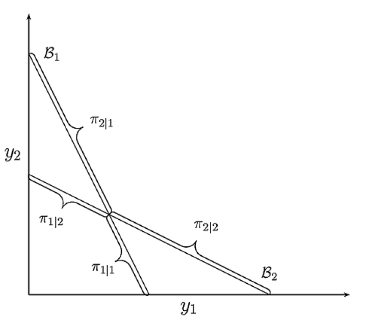
Figure 1. Example from Kitamura & Stoye (2018)

Assuming Walras’ Law, $\pi_{i|j}$ denotes the share of the decision-makers who choose in the segment $i$ from the budget set $\mathcal{B}_{j}$. Ignoring the intersection, the choice probabilities in this example are described by the vector $(\pi_{1|1},\pi_{2|1},\pi_{1|2},\pi_{2|2})$. There are four possible pairs of choices that the decision-makers can make and only one of them is irrational, i.e. $\pi_{1|1},\pi_{1|2}$. By similar reasoning as in our Example 1, this setting does not admit I-RUMs, but only pI-RUMs. Nonetheless, our discussion of the paradox of stochastic rationality easily follows.

First, suppose we observe the stochastically rational choice probabilities $(\pi_{1|1},\pi_{2|1},\pi_{1|2},\pi_{2|2})=(0.5,0.5,0.5,0.5)$. This RUM is a pI-RUM where the fraction of irrational decision-makers is at most 50%. The contingency tables below display two possible scenarios in which either 0% or 50% of the decision-makers are irrational. One can also note that not only this RUM is a pi-RUM, but there is only one representation in which every decision-maker is rational, while there is an infinity of representations in which at least some decision-makers are irrational. In the contingency tables, we color the irrational choices in red and the rational ones in blue.

$$\left[\begin{array}[]{c| cc | c}&\pi_{1|1}&\pi_{2|1}&\\ \hline\cr\pi_{1|2}&{\color[rgb]{1,0,0}0.5}&{\color[rgb]{0,0,1}0}&0.5\\ \pi_{2|2}&{\color[rgb]{0,0,1}0}&{\color[rgb]{0,0,1}0.5}&0.5\\ \hline\cr&0.5&0.5&1\end{array}\right]\left[\begin{array}[]{c| cc | c}&\pi_{1|1}&\pi_{2|1}&\\ \hline\cr\pi_{1|2}&{\color[rgb]{1,0,0}0}&{\color[rgb]{0,0,1}0.5}&0.5\\ \pi_{2|2}&{\color[rgb]{0,0,1}0.5}&{\color[rgb]{0,0,1}0}&0.5\\ \hline\cr&0.5&0.5&1\end{array}\right]$$

Imagine now to observe the following non-stochastically rational choice probabilities: $(\pi_{1|1},\pi_{2|1},\pi_{1|2},\pi_{2|2})=(1,0,0.1,0.9)$. A rapid inspection will reveal that the fraction of irrational decision-makers is both at least and at most 10% and that the unique RCM that produces the choice probabilities is:

$$\left[\begin{array}[]{c| cc | c}&\pi_{1|1}&\pi_{2|1}&\\ \hline\cr\pi_{1|2}&{\color[rgb]{1,0,0}0.1}&{\color[rgb]{0,0,1}0}&0.1\\ \pi_{2|2}&{\color[rgb]{0,0,1}0.9}&{\color[rgb]{0,0,1}0}&0.9\\ \hline\cr&1&0&1\end{array}\right]$$

This simple example reveals a couple of interesting facts. First, statistical tests that focus solely on the distance between the observed aggregate choice probabilities and the set of RUMs may lose relevant information regarding the rationality of the underlying behavior of the decision-makers. Second, as noticed by Im & Rehbeck (2022), assuming individual rationality implies the identification of 50% of the population with a high (resp. low) marginal rate of substitution between the two goods while relaxing this assumption opens to the possibility (identification of the joint distribution is now lost) that 100% of the individuals has a mild marginal rate of substitution with 50% of them being rational and 50% irrational. Clearly, welfare conclusions may differ substantially between these two scenarios.

7. Concluding remarks

In the last decades, economics has welcomed several critiques of its rational foundations. Being located within the literature on individual decision-making, our paper fits within this tendency as we have provided a characterization of the set of populations that are rational at an aggregate level and can be also represented as irrational ones at an individual level.

In these concluding remarks, we touch on a different and more positive viewpoint of our paper borrowed from Becker (1962): ”Economic theory is much more compatible with irrational behavior than had been previously suspected.” In our characterization results, we not only show that rational aggregate choices may be individually fully irrational but also that the aggregation of individually irrational behaviors may well be stochastically rational and that individuals with correlated mistakes can never be translated into rational aggregate behavior. These observations resonate within the framework of standard economic theory where market efficiency is built upon uncorrelated errors of individual investors.

Appendix A Auxiliary results

A.1. Preliminaries on convex analysis

A set $X\subset\mathbb{R}^{d}$ is convex if for all $x,y\in X$ and $\alpha\in(0,1)$ it holds that $\alpha x+(1-\alpha)y\in X$. The convex hull of a set $Y\subseteq\mathbb{R}^{d}$ is the intersection of all convex sets containing $Y$ and is denoted $\text{conv}(Y)$, or equivalently the set of all points that can be obtained as convex combinations of points from $Y$. A point $x\in X\subseteq\mathbb{R}^{d}$ is called an extreme point of $X$ if there is no $\alpha\in(0,1)$ and $y,z\in X\setminus\{x\}$ with $y\neq z$ such that $x=\alpha y+(1-\alpha)z$. In words, a point $x\in X$ is an extreme point if it cannot be written as a non-trivial convex combination of two other distinct points in $X$. Denote the set of extreme point of a convex set $X$ by $\text{ext}(X)$. The next result is a basic result from convex analysis (Rockafellar, 1970, p.155) and will be employed when showing sufficiency of the Fréchet bounds in theorem 4.1.

Lemma A.1.

(Carathéodory’s theorem) Every point $x$ in a convex set $X\subseteq\mathbb{R}^{d}$ can be written as a convex combination of the extreme points of $X$. I.e. $\text{conv}(\text{ext}(X))=X$.

A.2. Preliminaries on stochastic rationality and Block-Marschak polynomials

The well-known characterization of the RUM is based on the Block-Marschak-polynomials (BM-polynomials). Define for all $A\subseteq X$ and $a\in X$ the BM-polynomial at $a$ in $A$ by:

$$\text{BM}_{\rho}(a,A)=\sum_{A\subseteq B\subseteq X}(-1)^{|B\setminus A|}\rho(a,B)$$

Theorem A.2 (Block & Marschak (1960), Falmagne (1978), Barberá & Pattanaik (1986), Monderer (1992), Fiorini (2004)).

$\rho$ is a RUM if and only if $\text{BM}_{\rho}(a,A)\geq 0$ for all $A\subseteq X$ and $a\in X$.

We now state two facts about BM-polynomials. The first shows that the BM polynomials act as a convex operator on the set of stochastic choice functions.

Lemma A.3.

Let $\alpha\in(0,1)$ and $\rho,\rho^{\prime}$ be stochastic choice functions then

$$\text{BM}_{\alpha\rho+(1-\alpha)\rho^{\prime}}(a,A)=\alpha\text{BM}_{\rho}(a,A)+(1-\alpha)\text{BM}_{\rho^{\prime}}(a,A)$$

for all $a\in A$ and $A\subseteq X$.

Proof.

The proof is simple and follows by expanding the definition of a BM polynomial. We have that

$$\text{BM}_{\alpha\rho+(1-\alpha)\rho^{\prime}}(a,A)=\sum_{A\subseteq B\subseteq X}(-1)^{|B\setminus A|}\left[\alpha\rho(a,B)+(1-\alpha)\rho^{\prime}(a,B)\right]=$$

$$\alpha\sum_{A\subseteq B\subseteq X}(-1)^{|B\setminus A|}\rho(a,B)+(1-\alpha)\sum_{A\subseteq B\subseteq X}(-1)^{|B\setminus A|}\rho^{\prime}(a,B)=$$

$$\alpha\text{BM}_{\rho}(a,A)+(1-\alpha)\text{BM}_{\rho^{\prime}}(a,A).$$

∎

The second shows that RUMs with full support are characterized by strictly positive BM-polynomials.

Lemma A.4.

A RUM is full support if and only if $\text{BM}_{\rho_{\mu}}(a,A)>0$ for all $a\in A$ and $A\subseteq X$.

Proof.

This result follows from the discussion in (Turansick, 2022, p.7) ∎

A.3. Preliminaries on Fréchet bounds

The Fréchet bounds govern the relationship between joint and marginal distributions. Specifically, they come as bounds on the joint distribution given the marginals. In a general setting, the Fréchet bounds are obtained as follows.

Lemma A.5.

Let $\Omega$ be a sample space and $P:\Omega\to[0,1]$ a probability measure. For any finite collection of events $E_{1},...,E_{K}\subseteq\Omega$ it then holds that

$$\max\{0,\sum_{k=1}^{K}P(E_{k})-(K-1)\}\leq P(\cap_{k=1}^{K}E_{k}).$$

The Fréchet bounds follows from the basic laws of probability and an induction argument. In RCMs, $\mu$ is the joint distribution while $\rho_{\mu}$ is the marginal distribution, and the operation $\rho(c(A),A)=\mu(\{c^{\prime}\in\mathbb{C}:c^{\prime}(A)=c(A)\})$ is nothing more than a marginalization. The following result is hence a direct corollary to lemma A.5.

Lemma A.6.

Let $\rho$ be a stochastic choice function, $c$ be a choice function, and $\mathcal{B}$ be an arbitrary collection of choice sets. It then holds that

$$\max\{0,\sum_{A\in\mathcal{B}}\rho(c(A),A)-(|\mathcal{B}|-1)\}\leq\mu(\cap_{A\in\mathcal{B}}\{c^{\prime}\in\mathcal{C}:c^{\prime}(A)=c(A)\})$$

for all RCMs $\mu$ such that $\rho=\rho_{\mu}$.

It should be noted that the lefthand side of the above inequality is independent of the RCM $\mu$ that represents $\rho$. For our purposes, it is also instructive to consider the special case of lemma A.6 when $\mathcal{B}$ is the collection of all non-empty and non-singleton menus of $X$, i.e. when $\mathcal{B}=\{A\subseteq X:|A|\geq 2\}$ and $K=|\mathcal{B}|$. Then, since $\cap_{A\in\mathcal{B}}\{c^{\prime}\in\mathcal{C}:c^{\prime}(A)=c(A)\}=\{c\}$ we have the following result.

Lemma A.7.

Let $c$ be a choice function then it holds that

$$\max\{0,\sum_{A\in\mathcal{B}}\rho(c(A),A)-(K-1)\}\leq\mu(c)$$

for all RCMs $\mu$ such that $\rho=\rho_{\mu}$.

By this formulation of the Fréchet bounds it is clear that if the left-hand side of the inequality is strictly positive, then any $\mu$ that represents $\rho$ must assign (strictly) positive probability to the choice function on the right-hand side of the inequality. In particular, if $c$ is rationalizable then any RCM $\mu$ must assign positive probability to $c$, implying that $\rho_{\mu}$ is not an I-RUM. Equivalently, if a RUM has an irregular representation, so that $\mu(P)=0$ for all preferences $P$, then lemma A.7 implies the following bounds.

Weak correlation bounds. A stochastic choice function $\rho$ satisfies the weak correlation bounds if for all preferences $P$ it holds that

$$\frac{1}{K-1}\sum_{A\subseteq X:|A|\geq 2}\rho(c_{P}(A),A)\leq 1.$$

Although Lemma A.7 implies that the weak correlation bounds are necessary for an irrational representation they are not quite sufficient. The following example illustrates.

Example 6.

Let $\mu(aP_{1}bP_{1}c)=\mu(aP_{2}cP_{2}b)=0.4$, $\mu(bP_{3}cP_{3}a)=\mu(cP_{4}bP_{4}a)=0.1$. The following $p_{\mu}$ arises: $\rho_{\mu}(a,X)=\rho_{\mu}(a,ab)=\rho_{\mu}(a,ac)=0.8$, $\rho_{\mu}(b,bc)=0.5$. The two choice functions $c_{P_{1}},c_{P_{2}}$ related to $P_{1},P_{2}$ are salient and they both satisfy the weak correlation bounds.

$$\sum_{A\subseteq X:|A|\geq 2}\rho(c_{P_{1}}(A),A)=\sum_{A\subseteq X:|A|\geq 2}\rho(c_{P_{2}}(A),A)=2.9<K-1=3$$

However, one can easily see that if $\mu^{\prime}$ is an RCM with $\mu^{\prime}(c_{P_{1}})=\mu^{\prime}(c_{P_{2}})=0$ then $\rho$ cannot be represented by $\mu^{\prime}$ (i.e. $\rho\neq\rho_{\mu^{\prime}}$).

The problem in the above example is that $P_{1}$ and $P_{2}$ are close to being the same preference since they agree on the choices from all menus except $\{b,c\}$ (which contains the worst two alternatives of both orders). Moreover, a large fraction of the overall probability is assigned to $P_{1}$ and $P_{2}$ (i.e. probability $0.8$) and hence the stochastic choice function $\rho_{\mu}$ exhibits a high degree of correlation. It turns out that a slight variation of these bounds, namely the correlation bounds of section 3, are sufficient for an irrational representation of RUM.

Before providing the proof of theorem 4.1, we would like to briefly motivate the use of the word ”correlation” which intends a measure of concordance between the choices of the decision-makers in the population w.r.t. to a specific choice function. To see this, note that, w.r.t to a choice function $c$, we can split the probability mass in $\rho$ between the one that ”correlates” and ”uncorrelates” with $c$.

$$\frac{1}{K-1}\bigg{[}\underbrace{\sum_{A\subseteq X:|A|\geq 2}\rho(c(A),A)}_{\text{"correlation" $(\hat{\mathbb{C}}^{\rho}_{c})$}}+\underbrace{\sum_{A\subseteq X:|A|\geq 2}\rho(A\setminus c(A),A)}_{\text{"uncorrelation" $(\hat{\mathbb{U}}^{\rho}_{c})$}}\bigg{]}=1$$

Finally, we note that $\hat{\mathbb{C}}^{\rho}_{c},\hat{\mathbb{U}}^{\rho}_{c}\in[0,1]$ and the equation above implies $\hat{\mathbb{C}}^{\rho}_{c}-\hat{\mathbb{U}}^{\rho}_{c}\in[-1,1]$. An intuitive ”correlation” interpretation comes after noticing the relationship with the notion of Kendall rank correlation as $\hat{\mathbb{C}}^{\rho}_{c}$ is the probability mass on the choices that are concordant with $c$ while $\hat{\mathbb{U}}^{\rho}_{c}$ is the probability mass on the choices that are discordant with $c$, and $\frac{1}{K-1}$ is the normalization factor.

Appendix B Proof of theorem 4.1

B.1. The necessity of the Correlation bounds

The necessity of the Correlation bounds follows by an application of the Fréchet bounds in lemma A.6. Recall that $\mathcal{A}(P)=\{A\subseteq X:|A|\geq 2\}\setminus\{\{x_{P}(N-1),x_{P}(N)\}\}$ and $|\mathcal{A}(P)|=K-1$ for all preferences $P$. The following lemma is a special case of lemma A.6 and it follows by noting that for each preference $P$ we have $\cap_{A\in\mathcal{A}(P)}\{c\in\mathcal{C}:c(A)=c_{P}(A)\}=\{c_{P},c_{Q}\}$ where $Q$ agrees with $P$ on all the menus in $\mathcal{A}(P)$.

Lemma B.1.

Let $\rho$ be a stochastic choice function, $P$ be a preference, and $Q$ be a preference that agrees with $P$ on all menus in $\mathcal{A}(P)$. It then holds that

$$\max\{0,\sum_{A\in\mathcal{A}(P)}\rho(c_{P}(A),A)-(K-2)\}\leq\mu(\{c_{P},c_{Q}\})$$

for all RCMs $\mu$ such that $\rho=\rho_{\mu}$.

Since, any I-RUM $\mu$ puts zero probability on all the rational choice functions, i.e. $\mu(c_{P})=0$ for all preferences $P$, lemma B.1 implies that any I-RUM must satisfy the following inequalities for all preferences $P$:

$$\mathbb{C}^{\rho}_{P}=\frac{1}{K-2}\sum_{A\in\mathcal{A}(P)}\rho(c_{P}(A),A)\leq 1,$$

which are exactly the correlation bounds. The preceding discussion thus implies that the correlation bounds are necessary for an I-RUM representation.

B.2. The sufficiency of the Correlation bounds

We refer to the main text for an exposition and sketch of the general idea behind the proof. Let $\rho$ be a RUM with distribution $\mu$. We say that $\rho$ satisfies the Correlation bounds with strict inequality if $\mathbb{C}^{\rho}_{P}<1$ for all preferences $P$. Similarly we say that $\rho$ satisfies the Correlation bounds with equality if $\mathbb{C}^{\rho}_{P}=1$ for some preference $P$ and $\mathbb{C}^{\rho}_{P^{\prime}}\leq 1$ for all preferences $P^{\prime}$.

Lemma B.2.

The subset of RUMs that satisfy the Correlation bounds is a convex set. I.e. the set of all RUMs $\rho$ such that

$$\mathbb{C}^{\rho}_{P}\leq 1$$

for all preferences $P$ is convex.

Proof.

Let $\rho^{\prime},\rho^{\prime\prime}$ be RUMs with distributions $\mu^{\prime},\mu^{\prime\prime}$ that satisfy the Correlation bounds and let $\alpha\in(0,1)$. We claim that $\rho=\alpha\rho^{\prime}+(1-\alpha)\rho^{\prime\prime}$ satisfies the Correlation bounds. For all preferences $P$ we have $\mu(P)=\alpha\mu^{\prime}(P)+(1-\alpha)\mu^{\prime\prime}(P)$. Hence

$$(K-2)\mathbb{C}^{\rho}_{P}=\sum_{P^{\prime}\in\mathcal{P}}\mu(P^{\prime})n(P,P^{\prime})=\sum_{P^{\prime}\in\mathcal{P}}\left[\alpha\mu^{\prime}(P)+(1-\alpha)\mu^{\prime\prime}(P)\right]n(P,P^{\prime})$$

$$=\alpha\sum_{P^{\prime}\in\mathcal{P}}\mu^{\prime}(P^{\prime})n(P,P^{\prime})+(1-\alpha)\sum_{P^{\prime}\in\mathcal{P}}\mu^{\prime\prime}(P^{\prime})n(P,P^{\prime})=$$

$$=(K-2)\left[\alpha\mathbb{C}^{\rho^{\prime}}_{P}+(1-\alpha)\mathbb{C}^{\rho^{\prime\prime}}_{P}\right]\leq K-2$$

where the last inequality holds since $\mathbb{C}^{\rho^{\prime}}_{P},\mathbb{C}^{\rho^{\prime\prime}}_{P}\leq 1$ for all preferences $P$.

∎

Lemma B.3.

Every Dual RUM that satisfies the Correlation bounds with equality is an I-RUM.

Proof.

Let $\mu$ be a dual RUM with support on $\{P_{1},P_{2}\}$. Assume that $\mu(P_{1})\leq\mu(P_{2})$ and that $\mu(P_{1})n(P_{2},P_{1})+\mu(P_{2})n(P_{2},P_{2})=K-2$. Rearranging the latter equality it follows that $\mu(P_{2})=\frac{K-2-n(P_{2},P_{1})}{K-1-n(P_{2},P_{1})}$. Let $k\in\mathbb{N}$ be such that $k\mu(P_{1})=\mu(P_{2})$. I.e. $k=K-2-n(P_{2},P_{1})$. Order the elements of $\{A\in\mathcal{A}(P_{2}):c_{P_{2}}(A)\neq c_{P_{1}}(A)\}$ (which has cardinality $k+1$) as $A_{1},...,A_{k+1}$. For each $i\in\{1,...,k+1\}$ define a choice function $c^{\prime}_{i}$ by

$$c^{\prime}_{i}(A)=\begin{cases}c_{P_{1}}(A)&\text{if $A=A_{i}$}\\ c_{P_{2}}(A)&\text{if $A\neq A_{i}$}\\ \end{cases}$$

We next show that each $c^{\prime}_{i}$ is irrational. Since $A_{i}\neq\{x_{P_{2}}(N-1),x_{P_{2}}(N)\}$, it follows that $x_{P_{2}}(K)\in A_{i}$ for some $K<N-1$. Let $K^{*}$ be the smallest such $K$. If $A_{i}=\{x_{P_{2}}(K^{*}),...,x_{P_{2}}(N)\}$. Then $c^{\prime}_{i}(A_{i})=c_{P_{1}}(A_{i})\neq c_{P_{2}}(A_{i})=x_{P_{2}}(K^{*})$ but $c^{\prime}_{i}(\{x_{P_{2}}(K^{*}),x_{P_{2}}(K^{*}+1)\})=c_{P_{2}}(\{x_{P_{2}}(K^{*}),x_{P_{2}}(K^{*}+1)\})=x_{P_{2}}(K^{*})$. A violation of Sen’s property $\alpha$. If $A_{i}\subset\{x_{P_{2}}(K^{*}),...,x_{P_{2}}(N)\}$ then $c^{\prime}_{i}(\{x_{P_{2}}(K^{*}),...,x_{P_{2}}(N)\})=c_{P_{2}}(\{x_{P_{2}}(K^{*}),...,x_{P_{2}}(N)\})=x_{P_{2}}(K^{*})$ and $c^{\prime}_{i}(A_{i})=c_{P_{1}}(A_{i})\neq c_{P_{2}}(A_{i})=x_{P_{2}}(K^{*})$. A violation of Sen’s property $\alpha$.

Let $\mu^{\prime}$ be the uniform distribution on $c^{\prime}_{1},...,c^{\prime}_{k+1}$, i.e.

$$\mu^{\prime}(c^{\prime}_{i})=\frac{1}{k+1}$$

for all $i\in\{1,...,k+1\}$. To show that $\mu$ is an I-RUM, it remains to show that the stochastic choices generated by $\mu$ and $\mu^{\prime}$ are the same. There are two cases.

Case 1: If $A\neq A_{i}$ for all $i\in\{1,...,k+1\}$ then $c^{\prime}_{i}(A)=c_{P_{2}}(A)=c_{P_{1}}(A)$ for all $i\in\{1,...,k+1\}$ and it is clear that the stochastic choices generated by $\mu$ and $\mu^{\prime}$ are the same (i.e. that $\rho_{\mu}=\rho_{\mu^{\prime}}$).

Case 2: If $A=A_{i}$ for some $i\in\{1,...,k\}$. Then $c^{\prime}_{i}(A)=c_{P_{1}}(A)$ and $c^{\prime}_{j}(A)=c_{P_{2}}(A)$ for all $j\neq i$. It hence follows that

$$\sum_{j=1}^{n}\mu^{\prime}(c^{\prime}_{j})\mathbb{1}\{a=c^{\prime}_{j}(A)\}=\frac{1}{k+1}\mathbb{1}\{a=c^{\prime}_{i}(A)\}+\sum_{j\neq i}^{n}\frac{1}{k+1}\mathbb{1}\{a=c^{\prime}_{j}(A)\}=$$

$$=\frac{1}{k+1}\mathbb{1}\{a=c_{P_{1}}(A)\}+\frac{k}{k+1}\mathbb{1}\{a=c_{P_{2}}(A)\}$$

$$=\mu(P_{1})\mathbb{1}\{a=c_{P_{1}}(A)\}+\mu(P_{2})\mathbb{1}\{a=c_{P_{2}}(A)\},$$

where the last equality follows since $k\mu(P_{1})=\mu(P_{2})$ implies that $\mu(P_{1})=\frac{1}{k+1}$ and $\mu(P_{2})=\frac{k}{k+1}$. ∎

Lemma B.4.

Let $\mu$ be a RUM such that the correlation bounds are satisfied with equality. Then there are Dual RUMs $(\hat{\mu_{i}})_{i=1}^{n}$ such that

1. $\mu$ is a convex combination of the $(\hat{\mu_{i}})_{i=1}^{n}$, i.e. there are weights $\delta_{i}$ s.t. $\mu=\sum_{k=1}^{n}\delta_{i}\hat{\mu_{i}}$,

2. each Dual RUM $\hat{\mu_{i}}$ satisfies the correlation bounds with equality.

Proof.

Order the set of preferences as $\{P_{0},...,P_{n}\}$. Let $\mu$ be a RUM that satisfies the correlation bounds with equality. W.l.o.g. assume that the correlation bound is satisfied with equality at $P_{0}$ (i.e. we have $K-2=\sum\limits_{i=0}^{n}n(P_{0},P_{i})\mu(P)$). We next construct a series of Dual RUMs that satisfies (1) and (2) in the statement of the lemma.

For each $i\in\{1,...,n\}$ we define a dual RUM $\hat{\mu}_{i}$ with support on $\{P_{0},P_{i}\}$ and such that the correlation bounds are satisfied with equality

$$\hat{\mu}_{i}(P_{0})=\frac{K-2-n(P_{0},P_{i})}{K-1-n(P_{0},P_{i})}$$

$$\hat{\mu}_{i}(P_{i})=\frac{1}{K-1-n(P_{0},P_{i})}$$

The weights $(\delta_{i})_{i=1}^{n}$ on the Dual RUMs are then defined for each $i\in\{1,...,n\}$ as follows:

$$\delta_{i}=\mu(P_{i})[K-1-n(P_{0},P_{i})]$$

We show that $\sum_{i=1}^{n}\delta_{i}=1$, i.e. that the $\delta_{i}$ are indeed weights (that $\delta_{i}\geq 0$ is obvious). We have that

$$\sum_{i=1}^{n}\delta_{i}=\sum_{i=1}^{n}\mu(P_{i})[K-1-n(P_{0},P_{i})]=$$

$$[K-1][1-\mu(P_{0})]-\sum_{i=1}^{n}n(P_{0},P_{i})\mu(P_{i})=$$

$$1+K-2-\sum_{i=0}^{n}n(P_{0},P_{i})\mu(P_{i})=1,$$

where the first equality follows by definition of the weights $\delta_{i}$, the second equality follows since $\sum_{i=1}^{n}\mu(P_{i})[K-1]=[K-1][1-\mu(P_{0})]$, the third equality follows by noting that $n(P_{0},P_{0})\mu(P_{0})=[K-1]\mu(P_{0})$ and rearranging, and the final equality follows since the correlation bound holds with equality at $P_{0}$.

It remains to show that $\mu$ is a convex combination of the Dual RUMs $(\hat{\mu}_{i})_{i=1}^{n}$ defined above. It is clear that for all $i\in\{1,...,n\}$ it holds that

$$\mu(P_{i})=\delta_{i}\hat{\mu}_{i}(P_{i})=\sum_{j=1}^{n}\delta_{j}\hat{\mu}_{j}(P_{i}),$$

where the first equality follows by construction of $\delta_{i}$ and $\hat{\mu}_{i}$, and the second equality follows since $\hat{\mu}_{j}(P_{i})=0$ for all $j\neq i$. Finally, we note that

$$\mu(P_{0})=1-\sum_{i=1}^{n}\mu(P_{i})=\sum_{i=1}^{n}[\delta_{i}-\delta_{i}\hat{\mu}_{i}(P_{i})]=$$

$$\sum_{i=1}^{n}\delta_{i}[1-\hat{\mu}_{i}(P_{i})]=\sum_{i=1}^{n}\delta_{i}\hat{\mu}_{i}(P_{0}).$$

∎

Lemma B.5.

Let $\rho$ be a RUM with distribution $\mu$ (so $\rho=\rho_{\mu}$) that satisfies the correlation bounds with strict inequality then $\rho$ is not an extreme point.

Proof.

Let $\mu$ be a RUM $\mu$ that satisfies the correlation bounds with strict inequality (i.e. $\mathbb{C}^{\rho}_{P}<1$ for all preferences $P$). Clearly, $\mu$ has support of cardinality greater or equal than two. Let $P_{1},P_{2}$ be two (distinct) preferences in the support of $\mu$. Let $\alpha$ be a distribution with support on $P_{1},P_{2}$ such that the Dual RUM $\rho^{d}$, defined for all $a\in A\subseteq X$ by

$$\rho^{d}(a,A)=\alpha(P_{1})\mathbb{1}\{a=\max(P_{1},A)\}+\alpha(P_{2})\mathbb{1}\{a=\max(P_{2},A)\},$$

satisfies the correlation bounds with equality (it could also be constructed to satisfy the correlation bounds with strict inequality, it is immaterial for the argument). For each $\beta\in(0,1)$ such that $\mu(P_{i})-\beta\alpha(P_{i})>0$ for all $i\in\{1,2\}$ (or equivalently $\beta<\min\{\frac{\mu(P_{1})}{\alpha(P_{1})},\frac{\mu(P_{2})}{\alpha(P_{2})}\}$) define a RUM $\mu^{*}_{\beta}$ by

$$\mu^{*}_{\beta}(P)=\begin{cases}\frac{\mu(P)-\beta\alpha(P)}{1-\beta}&\text{if $P\in\{P_{1},P_{2}\}$}\\ \frac{\mu(P)}{1-\beta}&\text{otherwise.}\end{cases}$$

Let $\rho^{*}(\beta)=\rho_{\mu^{*}_{\beta}}$, i.e. $\rho^{*}(\beta)$ is the RUM stochastic choice function with distribution $\mu^{*}_{\beta}$. For each preference $P$ define a function $f_{P}$ by

$$f_{P}(\beta)=\mathbb{P}^{\rho^{*}(\beta)}_{c_{P}}$$

for all $\beta\in[0,\min\{\frac{\mu(P_{1})}{\alpha(P_{1})},\frac{\mu(P_{2})}{\alpha(P_{2})}\})$. First note that $f_{P}(0)=\mathbb{C}^{\rho^{*}(0)}_{c_{P}}=\mathbb{C}^{\rho}_{c_{P}}$ for all preferences $P$. Hence, since the correlation bounds are satisfied with strict inequality we have $f_{P}(0)<1$ for all preferences $P$. Define a (vector-valued) function $f(\beta):=(f_{P}(\beta))_{P\in\mathcal{P}}$. Since each $f_{P}$ is a continuous function of $\beta$ it follows that $f$ is a continuous function of $\beta$ and hence there is a $\hat{\beta}>0$ such that $f_{P}(\beta)<1$ for all $0\leq\beta<\hat{\beta}$ and for all preferences $P$. Let $\beta$ be such that $0<\beta<\hat{\beta}<\min\{\frac{\mu(P_{1})}{\alpha(P_{1})},\frac{\mu(P_{2})}{\alpha(P_{2})}\}$. We then have that $\rho=\beta\rho^{d}+(1-\beta)\rho^{*}(\beta)$ and since both $\rho^{d}$ and $\rho^{*}(\beta)$ satisfy the correlation bounds, it follows that $\rho$ is not an extreme point (as it can be written as a non-trivial convex combination of two other RUMs that satisfy the correlation bounds). ∎

Appendix C Other proofs omitted from main text

C.1. Proof of Theorem 4.4

For each menu $A$ define a relation $\sim_{A}$ by $a\sim_{A}b$ if and only if $\rho(a,A)>0$ and $\rho(b,A)>0$. We will use these relations in the proof of theorem 4.4 below.

Proof.

We show that (1) $\Rightarrow$ (2) $\Rightarrow$ (3) $\Rightarrow$ (1).

(1) $\Rightarrow$ (2): By proposition 4.5 it follows that any RUM (hence any partial I-RUM) with support consisting of three or more preferences is a non-trivial convex combination of an I-RUM and a dual RUM. If $\rho$ is a partial I-RUM with support consisting of at most two preferences, then either $\rho$ is an I-RUM in which case it is a convex combination of itself (a dual RUM) and an I-RUM. Otherwise, $\rho$ is a convex combination of a preference (a degenerate dual RUM) and an irrational choice function.

(2) $\Rightarrow$ (3): It is clear that if (2) holds then $\rho_{\mu}$ is a partial I-RUM. Suppose that (3) is not true. We claim that there for every menu $B\subseteq X$ with $|B|\geq 3$ is a $c(B)$ with $\rho(c(B),B)=1$. If not then there are $a,b\in B$ with $\rho(a,B)>0$ and $\rho(b,B)>0$ and regularity of RUM then implies that $\rho(a,ab)>0$ and $\rho(b,ab)>0$. Hence $a\sim_{B}b$ and $a\sim_{ab}b$. A contradiction.

The previous paragraph implies that there is exactly one binary subset $\{a,b\}$ with $\rho(a,ab)>0$ and $\rho(b,ab)>0$. Assume, there is a binary subset $\{c,d\}\neq\{a,b\}$ with $\rho(c,cd)>0$ and $\rho(d,cd)>0$. By the previous paragraph there is an $x\in\{a,b,c,d\}$ with $\rho(x,abcd)=1$. Assume w.l.o.g. that $x=c$, then $1=\rho(c,abcd)\leq\rho(c,cd)$, implying that $\rho(d,cd)=0$. A contradiction.

(3) $\Rightarrow$ (1): Let $\rho$ be a stochastic choice function such that $\rho=\rho_{\mu}$ for some RUM $\mu$ and assume that there are $A,B\in\mathcal{A}$ and alternatives $a,b\in A\cap B$ with $a\sim_{A}b$ and $a\sim_{B}b$. We construct a partial I-RUM that represents $\rho$. Since there are $a,b\in A\cap B\subseteq X$ with $\rho(a,A)>0,\rho(b,A)>0$ and $\rho(a,B)>0,\rho(b,B)>0$, there is a $B\subseteq X$ with $|B|\geq 3$ and $a,b\in B$ such that $\rho(a,B)>0$ and $\rho(b,B)>0$. Let $P_{1}$ be a preference in the support of $\mu$ such that $\max(P_{1},B)=a$ and $P_{2}$ a preference in the support of $\mu$ such that $\max(P_{2},B)=b$. Assume w.l.o.g. that $\mu(P_{1})\leq\mu(P_{2})$. Construct choice functions $c^{\prime}_{1},c^{\prime}_{2}$ such that

$$c^{\prime}_{i}(A)=\begin{cases}\max(P_{i},A)&\text{if $A\neq B$}\\ \max(P_{j},A)&\text{if $A=B$}\\ \end{cases}$$

It is clear that both $c_{1}$ and $c_{2}$ are irrational. Let $\mu^{\prime}$ be an RCM such that $\mu^{\prime}(c_{P})=\mu(c_{P})$ for all $P\in\mathcal{P}\setminus\{P_{1},P_{2}\}$ and $\mu^{\prime}(c^{\prime}_{1})=\mu(c_{P_{1}})$ and $\mu^{\prime}(c^{\prime}_{2})=\mu(c_{P_{1}})$ and $\mu^{\prime}(c_{P_{2}})=\mu(c_{P_{2}})-\mu(c_{P_{1}})$. It is straightforward to check that $\mu^{\prime}$ represents $\rho$, i.e. that $\rho=\rho_{\mu^{\prime}}$ and hence it follows that $\rho$ is a partial I-RUM. ∎

C.2. Proof of proposition 4.5

Proof.

We prove the claim by induction on $k$ where $k$ is the cardinality of the support of the RUM.

Base cases ($k=1,2$). These cases are trivial as RUMs with support of cardinality smaller than two already satisfy the conclusion of the claim.

Induction hypothesis and induction step. As induction hypothesis assume that the claim is true for all $1\leq k<m$ (where $m>2$). To prove the induction step let $k=m$. Then the support of $\mu$ consists of preferences $P_{1},...,P_{m}$. Define an equivalence relation $\sim$ on $\{P_{1},...,P_{m}\}$ by $P_{i}\sim P_{j}$ if and only if $P_{i}$ and $P_{j}$ rank all alternatives, except the worst two, the same. Order the equivalence classes of $\sim$ as $E_{1},...,E_{n}$ where $\mu(E_{1})\leq...\leq\mu(E_{n})$ and $2\leq n\leq m$. Let $P_{11}$ be a preference in $E_{1}$ and $P_{22}$ a preference in $E_{2}$. Since $P_{11}$ and $P_{22}$ belong to different equivalence classes there is a set of three alternatives $\{a,b,c\}$ such that $\max(P_{11},\{a,b,c\})\neq\max(P_{22},\{a,b,c\})$. Define a choice function $c_{11}$ such that

$$c_{11}(A)=\begin{cases}\max(P_{11},A)&\text{if $A\neq\{a,b,c\}$}\\ \max(P_{22},A)&\text{if $A=\{a,b,c\}$}\\ \end{cases}$$

Similarly, define $c_{22}$ by

$$c_{22}(A)=\begin{cases}\max(P_{22},A)&\text{if $A\neq\{a,b,c\}$}\\ \max(P_{11},A)&\text{if $A=\{a,b,c\}$}\\ \end{cases}$$

It is straightforward to check that both of these choice functions are non-rational (as they violate WARP). Consider the RCM $\mu^{\prime}$ defined by $\mu^{\prime}(c_{11})=\mu(P_{11})$ and $\mu^{\prime}(c_{22})=\mu(P_{11})$ and with $\mu^{\prime}(c_{P_{22}})=\mu(P_{22})-\mu(P_{11})$ and $\mu^{\prime}(c_{P})=\mu(P)$ for all $P\in\{P_{1},...,P_{n}\}\setminus\{P_{11},P_{22}\}$. It is straightforward to check that $\rho_{\mu^{\prime}}(a,A)=\rho_{\mu}(a,A)$ for all $A\subseteq X$ and $a\in A$. Next, we note that we can write $\mu^{\prime}$ as a convex combination of $c_{11}$, $c_{22}$ and a RUM $\mu^{\prime\prime}$ with support of cardinality less than or equal to $m-1$. But this later RUM $\mu^{\prime\prime}$ can, by the induction hypothesis, be written as an RCM with support consisting of at most two preferences. The claim now follows. ∎

C.3. Proof of proposition 5.1

Proof.

Let $\mathtt{SCF}$ be the collection of all stochastic choice functions. Define a function $F:\mathtt{SCF}\to\mathbb{R}$ by

$$F(\rho)=\min_{a\in A:A\subseteq X}\text{BM}_{\rho}(a,A).$$

Viewing $\mathtt{SCF}$ as a convex subset of $\mathbb{R}^{d}$ (for suitable $d$) it is straightforward to check that $F$ is a continuous function (to see this, first note that $\text{BM}_{\rho}(a,A)$ is continuous for fixed $a\in A$ and $A\subseteq X$, and since the minimum of a finite number of continuous functions is continuous it follows that $F$ is continuous). Let $\mathtt{M}^{*}$ denote the closure of $\mathtt{M}$. Since $\mathtt{M}^{*}$ is compact and $F$ is continuous there is a $M>0$ such that $F(\rho)\geq-M$ for all $\rho\in\mathtt{M}^{*}$ (hence for all $\rho\in\mathtt{M}$). Since $\rho_{\mu}$ is a full support RUM there is an $\beta>0$ such that $\text{BM}_{\rho_{\mu}}(a,A)\geq\beta$ for all $a\in A$ and $A\subseteq X$. Let $1>\bar{\alpha}>0$ be large enough such that $\bar{\alpha}>\frac{M}{\beta+M}>0$ (such a number clearly exists). Let $\alpha\geq\bar{\alpha}$. We need to prove that $\rho^{*}=\alpha\rho_{\mu}+(1-\alpha)\rho$ is a RUM.

Let $\alpha\geq\bar{\alpha}$ and $\rho\in\mathtt{M}$. We need to prove that $\rho^{*}=\alpha\rho_{\mu}+(1-\alpha)\rho$ is a RUM. It suffices to show that the BM-polynomials of $\rho^{*}$ are non-negative. Let $a\in A$ and $A\subseteq X$. There are two cases.

Case 1. Assume first that $\text{BM}_{\rho}(a,A)\geq 0$. By lemma A.3 we then have

$$\text{BM}_{\rho^{*}}(a,A)=\alpha\text{BM}_{\rho_{\mu}}(a,A)+(1-\alpha)\text{BM}_{\rho}(a,A)\geq 0$$

Case 2. Assume next that $\text{BM}_{\rho}(a,A)<0$. Then

$$\text{BM}_{\rho^{*}}(a,A)=\alpha\text{BM}_{\rho_{\mu}}(a,A)+(1-\alpha)\text{BM}_{\rho}(a,A)\geq$$

$$\bar{\alpha}\text{BM}_{\rho_{\mu}}(a,A)+(1-\bar{\alpha})\text{BM}_{\rho}(a,A)\geq$$

$$\bar{\alpha}\beta+(1-\bar{\alpha})(-M)=\bar{\alpha}(\beta+M)-M>0.$$

The first (in)equality follows by lemma A.3 (i.e. convexity of the BM operator). The second (in)equality follows since $\alpha\geq\bar{\alpha}$ and $\text{BM}_{\rho_{\mu}}(a,A)>\text{BM}_{\rho}(a,A)$ and the third (in)equality follows since $\text{BM}_{\rho_{\mu}}(a,A)\geq\beta$ and since $\text{BM}_{\rho}(a,A)\geq F(\rho)\geq-M$. ∎

References

- Aguiar & Kashaev (2021) Aguiar, V. H., & Kashaev, N. (2021). Stochastic revealed preferences with measurement error. The Review of Economic Studies, 88(4), 2042–2093.
- Apesteguia et al. (2017) Apesteguia, J., Ballester, M. A., & Lu, J. (2017). Single-crossing random utility models. Econometrica, 85(2), 661–674.
- Arrow (1959) Arrow, K. J. (1959). Rational choice functions and orderings. Economica, 26(102), 121–127.
- Barberá & Pattanaik (1986) Barberá, S., & Pattanaik, P. K. (1986). Falmagne and the rationalizability of stochastic choices in terms of random orderings. Econometrica, (pp. 707–715).
- Becker (1962) Becker, G. S. (1962). Irrational behaviour and economic theory. Journal of Political Economy, (70), 1–13.
- Block & Marschak (1960) Block, H., & Marschak, J. (1960). Random orderings and stochastic theories of responses. Contributions to Probability and Statistics, (Stanford University Press).
- Blundell et al. (2003) Blundell, R. W., Browning, M., & Crawford, I. A. (2003). Nonparametric engel curves and revealed preference. Econometrica, 71(1), 205–240.
- Dardanoni et al. (2023) Dardanoni, V., Manzini, P., Mariotti, M., Petri, H., & Tyson, C. J. (2023). Mixture choice data: revealing preferences and cognition. Journal of Political Economy, 131(3), 687–715.
- Dardanoni et al. (2020) Dardanoni, V., Manzini, P., Mariotti, M., & Tyson, C. (2020). Inferring cognitive heterogeneity from aggregate choices. Econometrica, 88(3), 1269–1296.
- Deb et al. (2023) Deb, R., Kitamura, Y., Quah, J. K., & Stoye, J. (2023). Revealed price preference: theory and empirical analysis. The Review of Economic Studies, 90(2), 707–743.
- Falmagne (1978) Falmagne, J.-C. (1978). A representation theorem for finite random scale systems. Journal of Mathematical Psychology, 18(1), 52–72.
- Filiz-Ozbay & Masatlioglu (2023) Filiz-Ozbay, E., & Masatlioglu, Y. (2023). Progressive random choice. Journal of Political Economy, 131(3), 716–750.
- Fiorini (2004) Fiorini, S. (2004). A short proof of a theorem of falmagne. Journal of mathematical psychology, 48(1), 80–82.
- Gilboa (1990) Gilboa, I. (1990). A necessary but insufficient condition for the stochastic binary choice problem. Journal of Mathematical Psychology, 34(4), 371–392.
- Grandmont (1992) Grandmont, J.-M. (1992). Transformations of the commodity space, behavioral heterogeneity, and the aggregation problem. Journal of Economic Theory, 57(1), 1–35.
- Hoderlein & Stoye (2014) Hoderlein, S., & Stoye, J. (2014). Revealed preferences in a heterogeneous population. Review of Economics and Statistics, 96(2), 197–213.
- Hoderlein & Stoye (2015) Hoderlein, S., & Stoye, J. (2015). Testing stochastic rationality and predicting stochastic demand: the case of two goods. Economic Theory Bulletin, 3(2), 313–328.
- Im & Rehbeck (2022) Im, C., & Rehbeck, J. (2022). Non-rationalizable individuals and stochastic rationalizability. Economics Letters, 219, 110786.
- Kitamura & Stoye (2018) Kitamura, Y., & Stoye, J. (2018). Nonparametric analysis of random utility models. Econometrica, 86(6), 1883–1909.
- Luce & Raiffa (1957) Luce, R., & Raiffa, H. (1957). Introduction and critical survey.
- Manzini & Mariotti (2018) Manzini, P., & Mariotti, M. (2018). Dual random utility maximisation. Journal of Economic Theory, 177, 162–182.
- Matzkin (2007) Matzkin, R. L. (2007). Heterogeneous choice. Econometric Society Monographs, 43, 75.
- McCausland et al. (2020) McCausland, W. J., Davis-Stober, C., Marley, A. A., Park, S., & Brown, N. (2020). Testing the random utility hypothesis directly. The Economic Journal, 130(625), 183–207.
- McFadden & Richter (1990) McFadden, D., & Richter, M. K. (1990). Stochastic rationality and revealed stochastic preference. Preferences, Uncertainty, and Optimality, Essays in Honor of Leo Hurwicz, Westview Press: Boulder, CO, (pp. 161–186).
- McFadden (2006) McFadden, D. L. (2006). Revealed stochastic preference: a synthesis. In Rationality and Equilibrium: A Symposium in Honor of Marcel K. Richter, (pp. 1–20). Springer.
- Monderer (1992) Monderer, D. (1992). The stochastic choice problem: A game-theoretic approach. Journal of Mathematical Psychology, 36(4), 547–554.
- Petri (2023) Petri, H. (2023). Random (ordered) multivalued choice. Working paper.
-
Rockafellar (1970)
Rockafellar, R. T. (1970).
Convex Analysis.
Princeton: Princeton University Press.
URL https://doi.org/10.1515/9781400873173 - Sen (1971) Sen, A. (1971). Choice functions and revealed preference. The Review of Economic Studies, 38(3), 307–317.
- Smeulders et al. (2021) Smeulders, B., Cherchye, L., & De Rock, B. (2021). Nonparametric analysis of random utility models: computational tools for statistical testing. Econometrica, 89(1), 437–455.
- Stoye (2019) Stoye, J. (2019). Revealed stochastic preference: A one-paragraph proof and generalization. Economics Letters, 177, 66–68.
- Suleymanov (2023) Suleymanov, E. (2023). Branching-independent random utility model. Working paper.
- Turansick (2022) Turansick, C. (2022). Identification in the random utility model. Journal of Economic Theory, 203.