Dynamics, locality and weak measurements: trajectories and which-way information in the case of a simplified double-slit setup

Abstract

Understanding how the interference pattern produced by a quantum particle in Young’s double-slit setup builds up – the “only mystery” of quantum mechanics according to Feynman – is still a matter of discussion and speculation. Recent works have revisited the possibility of acquiring which-way information based on weak measurements. Weak measurements preserve the interference pattern due to their minimally perturbing character while still leading to a final position detection. Here we investigate a simplified double-slit setup by including weakly coupled pointers. We examine how the information provided by the weak pointers can be interpreted to infer the dynamics within a local picture through “weak trajectories”. We contrast our approach with non-local dynamical accounts, such as the modular momentum approach to weak values and the trajectories defined by the de Broglie-Bohm picture.

I Introduction

In the Character of Physical Law [1], Feynman discusses at length the double slit experiment. He asks whether it is true that “electrons must go either through one hole or another”. His answer is that if we look we will indeed find the electron at one slit or the other, but we will then loose the interference pattern. If we do not look, such a claim would be an “error”. Since then the weak measurement (WM) scheme, a minimally-disturbing process that enables one to gain information on the property of a quantum system at an intermediate time $t$ as the system evolves from an initially prepared state $|\psi(t_{i})\rangle$ to final state $|\chi(t_{f})\rangle$ has been proposed [2]. Although they are difficult to undertake experimentally, weak measurements have been observed, including in situations [3] calling for Feynman’s which slit (or, more generally, which-path) question. Such techniques open an observational window on the evolution of a quantum system between preparation and final detection.

Several recent works [4, 5, 6, 7, 8, 9, 10, 11] have employed weak measurements in the context of the double slit setup. One of the aims is to answer the which slit question, or rather more precisely to account for the slit traversal dynamics. One series of works [4, 7, 5, 10] focused on “weak trajectories” [12, 13, 9], that is trajectories that are defined by a series of weak measurements of the system’s position. These weak trajectories are related [14] to the sum over the Feynman paths of the system, so that one observes a superposition of trajectories going through each slit, with the constraint that these trajectories must be compatible with the post-selected quantum state at the detection point on the screen. Other works [8, 11] have focused more directly on the which-way question, that is whether by performing a weak measurement one can tell that an electron went though a given slit while maintaining interference at the detection screen. Employing a simplified setup taking into account the sole dimension along the slits (or equivalently the detection plane), Ref. [8] argues that it is possible to infer which slit the particle has gone through without destroying the interference pattern, while Ref. [11] argues, in line with the weak trajectories based results, that the particle is delocalized on both slits.

In this paper, we study the simplified setup employed in Ref. [8] with the tools introduced to investigate the full double slit setup in an earlier work by one of us [10], work whose aim was precisely to observe the superposition of paths coming from each slit at the detection screen. In the full, two-dimensional setup, a great number of interfering paths typically contribute to the weak values and to the final detection, rendering the analysis convoluted. In the simplified setup, the one-dimensional character of the problem makes it simple to capture the dynamics in terms of weak pointers interacting locally with the system and picking up the interference between two wavepackets.

The paper is organized as follows. We will first briefly review wavepacket propagation and the “weak trajectories” resulting from the interaction between the wavepacket and a series of weakly coupled pointers placed along the way (Sec. II). We will then introduce in Sec. III the simplified double-slit setup and derive the three types of weak values that may appear in this setup. Sec. IV will discuss how the dynamics can be inferred from these weak values. We will contrast the resulting local dynamics from the one supported by a non-local approach to the weak values [8, 15] based on a localized particle subjected to non-local potentials. We will also discuss the dynamical picture arising from the de Broglie-Bohm model [16, 17], that is well-known to be non-local; to this end, Bohmian trajectories in the presence of pointers will be computed numerically. Our concluding remarks will be given in Sec. V.

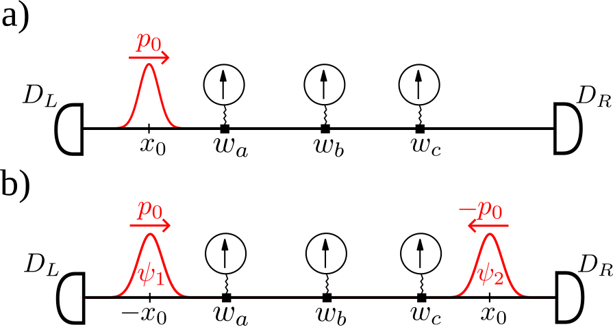
Figure 1: (a) Schematics of a wavepacket with initial mean position $x_{0}$ launched towards the detector $D_{R}$. The wavepacket will be detected by $D_{R}$ with certainty interacting along the way with weakly coupled pointers such as those positioned at $w_{a},w_{b},w_{c}$. The shifts of these pointers define the “weak trajectory” of the particle. (b) Simplified double-slit setup: The initial state is a superposition of two wavepackets $\psi_{1}$ and $\psi_{2}$ initially centered at $-x_{0}$ and $x_{0}$ resp. (mimicking the positions of the slits), and with initial momentum $p_{0}$ and $-p_{0}$. Post-selection takes place at $D_{R}$.

II Weak values and detection of a propagating wavepacket

II.1 Wavepacket evolution

Let us consider the following simple situation: a wavepacket initially $(t=0)$ centered at $x_{0}$ with mean momentum $p_{0}$ propagates freely towards the right $\left(p_{0}>0\right)$. Two detectors $D_{L}$ and $D_{R}$ are placed respectively at $x_{L}$ and $x_{R}$ lying to the left and to the right of the wavepacket’s initial position (see Fig. 1(a)). For definiteness we will choose the wavepacket $\psi_{G}(x,t)$ of the particle to be a Gaussian of width $d$, given under free Hamiltonian evolution by

$$\psi_{G}(x,t;x_{0},p_{0})=\frac{\left(\frac{2}{\pi}\right)^{1/4}\sqrt{dm}}{\left(2d^{2}m+i\hbar t\right)^{1/2}}\exp\left(-\frac{m(x-x(t))^{2}}{4d^{2}m+2i\hbar t}+\frac{ip_{0}\left(x-x(t)\right)}{\hbar}+\frac{ip_{0}^{2}t}{2\hbar m}\right)$$ (1)

where $x(t)=x_{0}+p_{0}t/m$ is the position of the center of the wavepacket ($m$ is the particle mass). Eq. (1) is obtained by applying the particle’s evolution operator $\hat{U}(t^{\prime},t)=e^{-i\frac{\hat{p}^{2}}{2m\hbar}(t^{\prime}-t)}$ to $\left|\psi_{G}((t=0)\right\rangle$. In the position representation, the evolution operator is given by the so called free propagator,

$$K(x^{\prime},t^{\prime};x,t)\equiv\left\langle x^{\prime}\right|\hat{U}(t^{\prime},t)|x\rangle=\left(\frac{m}{2i\pi\hbar(t^{\prime}-t)}\right)^{\frac{1}{2}}\hskip 1.42271pte^{\frac{im(x^{\prime}-x)^{2}}{2\hbar(t^{\prime}-t)}}$$ (2)

Once the wavepacket is launched, and if the wavepacket broadening is deemed to be negligible, the detector $D_{R}$ will click with certainty.

II.2 From weak values to weak trajectories

Let us now insert a pointer along the way between $x_{0}$ and $x_{R}$, say at $x=w_{1}$ and let us assume the coupling between the pointer and the particle is weak. More precisely, we will couple the probe momentum $\hat{P}$ to the particle observable $\hat{A}$. This implies that in addition to the particle’s free Hamiltonian, there is an interaction term of the form

$$\hat{H}_{int}=g(t)\hat{A}\hat{P}f_{w}.$$ (3)

$g(t)$ determines the timing at which the coupling is turned on, a function that will be non-vanishing only in a small interval centered on the interaction time $t_{w}$. $f_{w}$ reflects the short-range character of the interaction that is only non-vanishing in a small region near $w_{1}$. Since we are assuming the interaction is weak, the evolution due to $\hat{H}_{int}$ in the propagator is taken only to first order [14]. The system wavefunction $\psi_{G}$ is thus only slightly perturbed and continues to evolve until at time $t_{f}$ a standard measurement is made, leaving the system in a state $\left|\chi_{f}(t_{f})\right\rangle$ which is an eigenstate of the measured observable. The initial state of the pointer $\left|\phi_{i}\right\rangle$ becomes at $t_{f}$ $\left|\phi_{f}\right\rangle=e^{-igA^{w}\hat{P}}\left|\phi_{i}\right\rangle$ where $A^{w}$ is the weak value [2] given here by

$$A^{w}=\frac{\left\langle\chi_{f}(t_{f})\right|\hat{U}(t_{f},t_{w})\hat{A}\hat{U}(t_{w},t_{i})\left|\psi_{G}(t_{i})\right\rangle}{\left\langle\chi_{f}(t_{f})\right|\hat{U}(t_{f},t_{i})\left|\psi_{G}(t_{i})\right\rangle}$$ (4)

where $g=\int dt^{\prime}g(t^{\prime})$ (see [18] for a derivation employing the present notation). The final probe state is hence the initial one shifted by $g\operatorname{Re}(A^{w})$.

The weak value is defined provided the post-selected state $\left|\chi_{f}(t_{f})\right\rangle$ overlaps with the freely evolved particle state at time $t_{f}$ in line with the idea that the interaction is so weak as not to affect the detection probabilities. Here, let us set the pointer to couple to the spatial projector at $w_{1},$ $\hat{A}=\left|x_{1}\right\rangle\left\langle x_{1}\right|$, $D_{R}$ will click almost with certainty provided post-selection captures exactly the (unperturbed) system wavefunction.  This is tantamount to choosing $\left|\chi_{f}(t_{f})\right\rangle=\left|\psi_{G}(t_{f})\right\rangle$ and the weak value is simply given by $\left|\psi_{G}(x_{w},t_{w})\right|^{2}.$ More realistically, $\hat{A}$ should be taken as a projector over a finite width [19] and the weak value would be given by $A^{w}=\int_{f_{w}}\left|\psi_{G}(x^{\prime},t_{w})\right|^{2}dx^{\prime}$ where the integration is over the domain defined by $f_{w}$. Finally, consider placing a series of identical weakly coupled pointers along the path from $x_{0}$ to $D_{R}$, choosing the time window at which the coupling is turned on. By tuning the time widow of each pointer so that it corresponds to the wavepacket going through the position of the pointer, one can observe – in principle experimentally, by measuring the pointers’ shift – the “weak trajectory” [13] of the system as it moves from $x_{0}$ to $D_{R}$.

Overall this gives a simple dynamical picture: recalling that the propagator $K$ of Eq. (2) can be written as a sum over the classical paths connecting $\left(x,t\right)$ to $\left(x^{\prime},t^{\prime}\right)$ – the term $m(x^{\prime}-x)^{2}/2(t^{\prime}-t)\$ is the classical action –, we see that the shift in each pointer can be understood as the result of the interaction between each pointer and the particle wavepacket propagating along the Feynman path connecting $x_{0}$ and $D_{R}$.

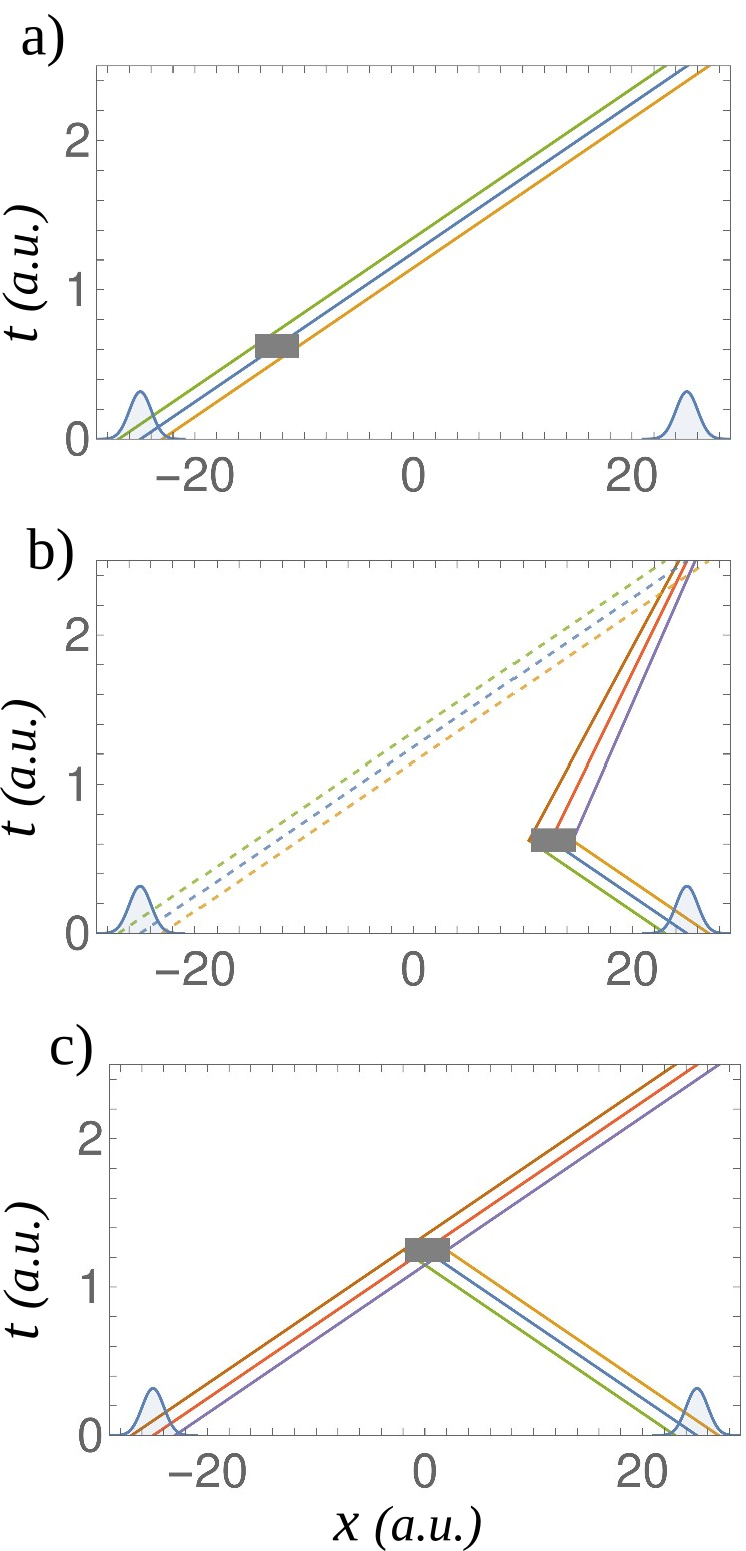
Figure 2: The three type of weak values mentioned in the text pictured with the corresponding weak trajectories; post-selection takes place at $D_{R}$ (we use atomic units and the system has unit mass). (a) The pointer placed at $w_{a}$ (gray box) interacts with the wave-packet initially centered at $-x_{0}$ (on the left) that will be postselected at $t_{f}$. (b) The weakly coupled pointer at $w_{c}$ interacts with the other wavepacket (originating from the right). The corresponding weak value will be non-zero if there are weak trajectories linking $w_{c}$ to the post-selection region at $D_{R}$. (c) The weak value at $w_{b}$ results from the superposition of both wavepackets.

III Weak values and post-selection in a simplified double-slit

III.1 The simplified double slit setup

Let us now take the scheme of the preceding section but choose instead the initial state as the superposition of two wavepackets initially on opposite sides and launched in opposite directions,

$$\psi(x,t=0)= \frac{1}{\sqrt{2}}\left(\psi_{G}(x,0;-x_{0},p_{0})-\psi_{G}(x,0;x_{0},-p_{0})\right)$$ (5)

$$\equiv \frac{1}{\sqrt{2}}\left(\psi_{1}(x,0)-\psi_{2}(x,0)\right)$$ (6)

This can be seen as the part of the wavefunction in the double-slit problem evolving in the plane of the slits. Recall indeed that the double-slit setup takes place in a two dimensional plane, but the wavefunction in the direction orthogonal to the detection plane is separable to a very good approximation [20, 10]. While Eq. (5) does not fully capture the dynamics of the two-slit problem, it pinpoints in a simpler way the “which slit” question: if the wavepacket is found say at $D_{R}$, can we say that this corresponds unambiguously to the part of the wavepacket $\psi_{1}$ that was initially located on the right (at $x_{0}$) ?

III.2 Weak values and post-selection

Consider Fig. 1(b), showing the position of 3 weakly coupled pointers $w_{a}$, $w_{b}$ and $w_{c}$ and let $t_{f}$ denote the average time it takes the wavepackets to reach a detector from its initial position. We post-select on $D_{R}$ at $t=t_{f}$ in all the cases – the post-selection hence involves only $\psi_{1}$. We will see that the weak values involve either a single wave-packet (which can only be $\psi_{1}$ given our post-selection choice) or a combination of $\psi_{1}$ and $\psi_{2}$.

Assume we turn on the pointer $a$ in a time-window centered on $t_{1}\simeq t_{f}/4$ when $\psi_{1}$, coming from the left, overlaps with $a$. The weak value is

$$\Pi_{a}^{w}(t_{1})=\frac{\left\langle\chi_{R}(t_{f})\right|\hat{U}(t_{f},t_{1})\left|w_{a}\right\rangle\left\langle w_{a}\right|\left.\psi_{1}(t_{1})\right\rangle}{\left\langle\chi_{R}(t_{f})\right|\left.\psi_{1}(t_{f})\right\rangle}.$$ (7)

For the moment the only assumption on $\left|\chi_{R}(t_{f})\right\rangle$ is that it is localized at the right detector $D_{R}$. The weak value (7) involves solely the $\psi_{1}$ part of the wavepacket (5), given that only $\psi_{1}$ interacts with $a$ at time $t_{1}$ ($\psi_{2}(w_{a},t_{1})$ vanishes) and is detected at $D_{R}$. Therefore, on this basis one might conclude that the particle detected by $D_{R}$ comes from the wavepacket initially localized at $x=-x_{0}$ near $D_{R}$. The Feynman paths contributing to $\Pi_{a}^{w}(t_{1})$ – the weak trajectories – are computed in Fig. 2(a); these paths are the classical trajectories, reaching the weak pointer at $t=t_{f}/4$ and the post-selection region at $t_{f}$.

However, consider turning on the pointer $c$ at the same time $t_{1}$, when the part $\psi_{2}$ of the wavepacket goes through it. The weak value is

$$\Pi_{c}^{w}(t_{1})=\frac{\left\langle\chi_{R}(t_{f})\right|\hat{U}(t_{f},t_{1})\left|w_{c}\right\rangle\left\langle w_{c}\right|\left.\psi_{2}(t_{1})\right\rangle}{\left\langle\chi_{R}(t_{f})\right|\left.\psi_{1}(t_{f})\right\rangle}.$$ (8)

Now both $\psi_{1}$ and $\psi_{2}$ contribute to the weak value, $\psi_{2}$ through the interaction with $c$ and $\psi_{1}$ by the post-selection condition. Note that for typical choices of $\left|\chi_{R}(t_{f})\right\rangle$, the term $\left\langle\chi_{R}(t_{f})\right|\hat{U}(t_{f},t_{1})\left|w_{c}\right\rangle$ does not vanish. Actually, if one chooses $\left|\chi_{R}(t_{f})\right\rangle=\left|x_{R}\right\rangle$, we have $\Pi_{c}^{w}(t_{1})=K(x_{R},t_{f};w_{c},t_{1})\psi_{2}(w_{c},t_{1})/\psi_{1}(x_{R},t_{f})$ that is seen to be proportional to the propagator. As is obvious from Eq. (2), the fact that there are classical trajectories linking $w_{c}$ to $x_{R}$ with momentum $\tilde{p}=\left(x_{R}-w_{c}\right)/\left(t_{f}-t_{1}\right)$ is enough to guarantee the non-zero character of the weak value, and hence the observation of a shifted pointer $c$. There are specific choices of $\left|\chi_{R}(t_{f})\right\rangle$ for which $\Pi_{c}^{w}(t_{1})$ could vanish – for example by imposing momentum filtering at $x_{R}$; indeed if $\left|\chi_{R}(t_{f})\right\rangle$ is chosen to be a Gaussian centered at $x_{R}$ with a mean momentum $p_{0}$ with a momentum distribution sufficiently narrow so as to exclude $\tilde{p}$, we will indeed obtain $\int dx^{\prime}\chi_{R}^{\ast}(x^{\prime},t_{f})K(x^{\prime},t_{f};w_{c},t_{1})\simeq 0$. But except for these specific choices, we see that we cannot say that the particle detected at $D_{R}$ came from the wavepacket $\psi_{1}$ coming from the left – given that the pointer $c$ shifts when turned on at time $t_{1}$. The difference with the single wavepacket case studied of Sec. II is that here post-selection is chosen at $D_{R}$ (thanks to $\psi_{1}$), whereas post-selection at $D_{L}$ was suppressed (up to order $g^{2}$) in the single wave-packet case. The paths contributing to this type of weak value are computed in Fig. 2(b).

Let us now focus on the pointer $b$ placed at the center. The interaction is turned on at $t_{2}$, and the weak value reads

$$\Pi_{b}^{w}(t_{2})=\sqrt{2}\frac{\left\langle\chi_{R}(t_{f})\right|\hat{U}(t_{f},t_{2})\left|w_{b}\right\rangle\left\langle w_{b}\right|\left.\psi(t_{2})\right\rangle}{\left\langle\chi_{R}(t_{f})\right|\left.\psi_{1}(t_{f})\right\rangle}.$$ (9)

Since the wavepackets interfere at $w_{b}$, the weak interaction couples contributions of both wavepackets to the pointer, as evidenced by the numerator. The corresponding paths are computed in Fig. 2(c). Typically $\Pi_{b}^{w}(t_{2})$ is non-zero, and the pointer shift can therefore be observed.

Let us finally combine the different couplings we can make with our 3 weak pointers. At $t_{1}$ we turn on the coupling for the pointers $a$ and $c$. Both pointers will detect the coupling, due to the interactions with $\psi_{1}$ and $\psi_{2}$ respectively [see Eqs. (7) and (8)]. If we turn all the pointers at $t_{2}$ (or additional pointers that would sit at $a$ and $c$, in order to preserve the quantum state of the pointers that had previously interacted at $t_{1}$), only the pointer $b$ interacts with the system, the pointer shift being proprotional to $\Pi_{b}^{w}(t_{2})$ [Eq. (9)]. At $t_{3}$ again both $a$ and $c$ interact with the system $\Pi_{a}^{w}(t_{3}),$ involving the interaction with $\psi_{2}$ is now of the type given by Eq. (8) and $\Pi_{c}^{w}(t_{3})$ similar to Eq. (7). After post-selection at $D_{R}$, combining the readings from all the weak pointers gives a view of the superposition of paths emanating both from the left $(-x_{0})$ and the right $(x_{0})$. These results call for a dynamical interpretation.

IV Inferring the dynamics from the weak values

IV.1 Weak trajectories: Local dynamics along Feynman paths

A particularly simple way of understanding the weak values determined in Sec. III is to follow the system evolution with Feynman paths. The weak value of the projector $\Pi_{w}=\left|w\right\rangle\left\langle w\right|$ at time $t_{w}$ depends [14] on the sum over paths connecting a point $x_{i}$ within the initial wavefunction $\psi(x_{i},t=0)$ to $w$ in time $t_{w}$ and then going from $w$ to a point $x_{f}$ of the final distribution $\left|\chi_{L}(x_{f},t_{f})\right|^{2}$ in time $t_{f}-t_{w}$. In our problem, the paths here are those carrying the wave-packet $\psi_{1}$ from the left towards $D_{R}$ interacting along the way with the pointers, as well as the paths carrying the wave-packet $\psi_{2}$ that get reflected by the interactions towards $D_{R}$. In terms of the analogy with the double-slit problem, we see that although post-selection is only compatible with the wave-packet $\psi_{1}$ having gone through slit 1, the weak values reflect nevertheless the presence of the wave having gone through the other slit, not only at the midpoint $b$ (with the corresponding weak value $\Pi_{b}^{w}(t_{2})$), but also at the other positions in which a weakly coupled pointer is placed: the corresponding weak trajectory starts at slit 2, and is turned back towards $D_{R}$ by the interaction.

Note that if there are no paths connecting $w$ to $x_{f}$ in time $t_{f}-t_{w}$ the weak value vanishes and the system does not leave any trace on the pointer. This can never happen for weak values of type 1 such as $\Pi_{a}^{w}(t_{1})$ given by Eq. (7) since  post-selection ensures that such paths exist. However for weak values of type 2 such as  $\Pi_{c}^{w}(t_{1})$, for which the interaction involves the wavepacket $\psi_{2}$ that is orthogonal to the post-selected one, it is always possible to choose the post-selected state so that the weak values of type 2 vanish. Since post-selection involves filtering, this can be done by finding a post-selection condition that filters away the paths (here imposing a momentum filtering function at post-selection by choosing an appropriate function $\chi_{R}(t_{f})$ would be the obvious choice). Recall that from a general standpoint, a zero weak value in a given region can mean different things [14]: (i) absence of the particle (when the interaction term in the classical Lagrangian vanishes in that region); (ii) a vanishing wavefunction by destructive interference of Feynman paths in that region; (iii) the wavefunction propagated by the paths affected by the interaction is orthogonal to the post-selection state (either the wavefunction does not reach the post-selection region or summing over the individual amplitudes results in a destructive interference). The latter case is at play when momentum filtering is imposed.

IV.2 Non-locality and modular momentum

A different take involving weak values in the same simplified double-slit problem was proposed recently by Aharonov et al [8]. The idea is to explain the interference pattern by way of a particle having a definite location but sensing non-locally the potential due to the other slit. Non-locality appears here through the evolution of the modular momentum operator, which depends both on the value of the potential at the particle position and on the value of the potential at a translated position (the position is translated by the reciprocal of the modulation [15], here the distance between the slits, i.e. between the mean positions of $\psi_{1}$ and $\psi_{2}$ at $t=0$). According to Ref. [8] this can explain the interference pattern produced (in our notation) when $\psi_{1}$ and $\psi_{2}$ overlap in the neighborhood of $b$ while at the same time one knows the path the particle took throughout given the post-selection condition.

Note however that asserting that the particle took a given path on the basis of post-selection only works for specific choices of post-selected states, those for which the weak values of type 2 mentioned above vanish. Otherwise the non-local dynamics must also account for the appearance of a non-zero weak value of type 2, that is for the fact that $\Pi_{c}^{w}(t_{1})\neq 0$ although the $\psi_{1}$ that will be post-selected is at $w_{a}$ at that time.

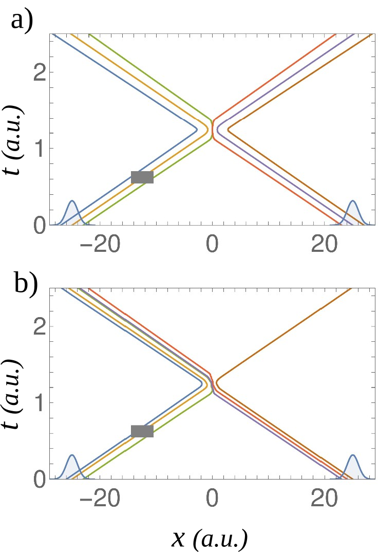
Figure 3: De Broglie-Bohm trajectories for the initial state given by Eq. (5) and an interaction with an interaction Hamiltonian given by Eq. (3) in a region centered at $w_{a}$. We use atomic units; the system has unit mass $m=1$, the pointer has a mass $M=10m$ and its initial state is represented by a Gaussian centered at $y=w_{a}$. (a) Weak coupling at $w_{a}$: the trajectories originating from $-x_{0}$ and $x_{0}$ and neighboring initial positions do not cross the midpoint, so that post-selection at $D_{R}$ is due to the trajectories having started on the right, at $x_{0}$ (all these trajectories are computed with the pointer having initial position $y=w_{a}$ a.u.). (b) With a stronger interaction (though not yet in the strong regime), some trajectories are seen to cross (all the trajectories are computed with the pointer having initial position $y=w_{a}-2$ a.u.

IV.3 The de Broglie-Bohm picture

The de Broglie Bohm (dBB) approach to the standard double slit problem is well-known [21, 16]: a point-like particle is assumed to go through one of the slits but its motion depends, through the quantum potential,while traveling along the current density arising from the wavefunction going through both slits. In the one-dimensional analog studied here, the dBB trajectories result from the interference between both wavepackets. In the absence of any interaction, the trajectories do not cross, given the symmetric character of the wavepackets [22]; the trajectories with initial position within $\psi_{1}$ evolve first towards the right but as they approach the midpoint they are turned back as the current density vanishes (due to $\psi_{1}$ and $\psi_{2}$ overlapping) and reverses its direction. This gives of course a dynamical interpretation that is radically different than the one given in terms of weak trajectories, since the post-selected particles at $D_{R}$ come from the right, not from the left.

If we now include interacting pointers, the numerical computation of Bohmian trajectories becomes more involved. We have computed in Fig. 3(a)-(b) the resulting trajectories when only the pointer $a$ is in place, and is turned on at $t_{1}$; we have taken the pointer wavefunction $\phi_{i}(y)$ to be given by a Gaussian (the computational details, based on an expansion of free standing waves in a box [23] will be given elsewhere). For a weak interaction Hamiltonian the dBB trajectories do not cross and are actually very similar to those in the no-interaction case – a consequence of the weakness of the coupling. For significantly stronger couplings some trajectories do cross. An example is shown in Fig. 3(b).

This paradoxical situation is reminiscent of other cases of mismatch between the intuitively expected dynamics and the alleged motion of the Bohmian particle (recall e.g., the case of surreal trajectories [24, 25], or the persistence of non-classical trajectories in semiclassical systems [26]). The model is nevertheless consistent if one assumes that the weak interaction with the quantum pointers does not involve the particle but only the pilot wave – the particle is only required to make detectors click, hence for strong measurements. If the interaction is made sufficiently strong so as to acquire which way information, then the Bohmian particle must interact with the pointer (given that the particle can be detected), but in the case of a strong interaction the Bohmian trajectories initially associated with $\psi_{1}$ do cross and are detected by $D_{R}$, a behavior that is quite general [27, 28].

V Conclusion

We have studied the dynamics that can be inferred from weak values in a simplified double-slit setup. While this simplified setup does not capture the entire set of issues that appear in full double-slit problem, it does bring to the fore the which-path question. Positioning weakly coupled pointers between the slits and the detection screen induces additional constraints on the dynamical picture, as the pointer shifts – given by the weak values – can in principle be measured. Nevertheless, these constraints are not sufficient to pin down unambiguously the dynamical evolution of the system. The choice between admitting a local picture with a delocalized superposition, or a localized particle subjected to non-local interactions remains open. It would be interesting to examine if, by considering more complex setups, some dynamical interpretations could be, if not ruled out impossible, rendered quite implausible.

References

- [1] R. P. Feynman, The Character of Physical Law (MIT Press, Cambridge, U.S., 1967).
- [2] Y. Aharonov, D. Z. Albert and L. Vaidman, Phys. Rev. Lett. 60, 1351 (1988).
- [3] S. N. Sahoo et al., Unambiguous joint detection of spatially separated properties of a single photon in the two arms of an interferometer, Comm. Phys. 6, 203 (2023).
- [4] T. Mori and I. Tsutsui, Quantum trajectories based on the weak value, PTEP 2015, 043A01 (2015).
- [5] L. P. Withers, Jr. and F. A. Narducci, Bilocal current densities and mean trajectories in a Young interferometer with two Gaussian slits and two detectors, J. Math. Phys. 56, 062106 (2015).
- [6] A. Luis and A. S. Sanz, What dynamics can be expected for mixed states in two-slit experiments?, Ann. Phys. 357, 95 (2015).
- [7] T. Mori and I. Tsutsui, Weak value and the wave–particle duality, Quantum Stud.: Math. Found. 2, 371 (2015).
- [8] Y. Aharonov et al., Finally making sense of the double-slit experiment, PNAS 114 6480 (2017).
- [9] R. Flack and B. J. Hiley, Feynman Paths and Weak Values, Entropy 20, 367 (2018).
- [10] Q. Duprey and A. Matzkin, Proposal to observe path superpositions in a double-slit setup, Phys. Rev. A 105, 052231 (2022).
- [11] H. F. Hofmann, T. Matsushita, S. Kuroki and M. Iinuma, A possible solution to the which-way problem of quantum interference, Quantum Stud.: Math. Found. 10 429 (2023).
- [12] A. Tanaka, Phys. Lett. A 297, 307 (2002).
- [13] A. Matzkin, Observing trajectories with weak measurements in quantum systems in the semiclassical regime, Phys. Rev. Lett. 109 150407 (2012).
- [14] A. Matzkin, Weak values from path integrals, Phys. Rev. Research 2, 032048(R) (2020).
- [15] Y. Aharonov, H. Pendleton and A. Petersen, Modular variables in quantum theory, Int J Theor Phys 2, 213 (1969).
- [16] P. R. Holland, The Quantum Theory of Motion (Cambridge University Press, Cambridge, 1993).
- [17] D. Bohm and B. J. Hiley, The Undivided Universe – An Ontological Interpretation of Quantum Theory (Routledge, London, 1993).
- [18] A. Matzkin, Weak Values and Quantum Properties, Found. Phys. 49, 298 (2019).
- [19] F. L. Traversa, G. Albareda, M. Di Ventra, and X. Oriols, Robust weak-measurement protocol for Bohmian velocities, Phys. Rev. A 87, 052124 (2013).
- [20] M. Beau, Feynman path integral approach to electron diffraction for one and two slits: analytical results, Eur. J. Phys. 33, 1023 (2012).
- [21] C. Philippidis, C. Dewdney and B. J. Hiley, Quantum interference and the quantum potential, 52, 15 (1979).
- [22] A. S. Sanz and S. Miret-Artes, A trajectory-based understanding of quantum interference, J. Phys. A: Math. Gen. 41, 435303 (2008).
- [23] A. Matzkin, Bohmian Mechanics, the Quantum-Classical Correspondence and the Classical Limit: The Case of the Square Billiard, Found Phys 39, 903 (2009).
- [24] B.-G. Englert, M. O. Scully, G. Sussmann, and H. Walther, Surrealistic Bohm Trajectories, Z. Naturforsch. 47a 1175 (1992).
- [25] L. Vaidman, The Reality in Bohmian Quantum Mechanics or Can You Kill with an Empty Wave Bullet?, Found. Phys. 35, 299 (2005).
- [26] A. Matzkin and V. Nurock, Classical and Bohmian trajectories in semiclassical systems: Mismatch in dynamics, mismatch in reality?, Studies in Hist. and Philosophy of Science B, 39, 17 (2008).
- [27] B. J. Hiley and R. E. Callaghan, Delayed-choice experiments and the Bohm approach, Phys. Scr. 74 336 (2006).
- [28] G. Tastevin and F. Laloe, Surrealistic Bohmian trajectories do not occur with macroscopic pointers, Eur. Phys. J. D 72, 183 (2018).