Finite temperature detection of quantum critical points via internal quantum teleportation

Abstract

We show that the teleportation protocol can be efficiently used to detect quantum critical points using finite temperature data even if all resources needed to its implementation lie within the system under investigation. Contrary to a previous proposal, there is no need to use an external qubit as the input state to be teleported to one of the qubits within the system. Here, we use a pair of nearest neighbor spins from an infinite spin-1/2 chain in equilibrium with a heat bath as the entangled resource of the quantum teleportation protocol and a third adjacent qubit within the chain itself as the input state to be teleported. For several spin chain models subjected to an external magnetic field, we show that the efficiency of the teleportation protocol is severely affected as we cross the quantum critical points associated with those spin chains. This abrupt change in efficiency gives us a clear indication of a quantum phase transition.

I Introduction

The qualitative change in the macroscopic properties of a many-body system that occurs at the absolute zero temperature ($T=0$) as we change its Hamiltonian is called a quantum phase transition (QPT). Theoretically it is described by the change of the many-body system’s ground state as we slowly (adiabatically) modify its Hamiltonian ($H$) sac99 ; gre02 ; gan10 ; row10 . Since at $T=0$ there are no thermal fluctuations, this change in the physical properties of the many-body system is caused by quantum fluctuations whose origin can be traced back to the Heisenberg uncertainty principle. A standard example of a QPT is the onset of a non-null magnetization when a spin chain enters its ferromagnetic phase coming from the paramagnetic one. In general, a QPT is given by a symmetry change in the ground state of the system and the appearance of an order parameter (the non-null magnetization in the above example).

Many important quantum information theory quantities were shown to be excellent quantum critical point (QCP) detectors at $T=0$ wu04 ; oli06 ; dil08 ; sar08 ; fan14 ; gir14 ; hot08 ; hot09 ; ike23a ; ike23b ; ike23c ; ike23d . However, it is known that some of them do not work properly when $T>0$. For example, the entanglement of formation woo98 between a pair of spins that belongs to a spin chain is zero before, at, and after the QCP if the chain is prepared above a certain threshold temperature wer10 ; wer10b . Therefore, both from a theoretical point of view and from practical aspects (we cannot cool a many-body system to $T=0$ due to the third law of thermodynamics), it is important to develop robust tools to characterize QPTs at finite $T$. In this case thermal fluctuations are present and we must have tools to detect QCPs that properly work in this scenario.

One of the most successful and resilient tool to pinpoint a QCP at finite $T$ is quantum discord (QD) wer10b , originally defined in Refs. oll01 ; hen01 . From a theoretical point of view, though, the computation of QD is not feasible for high spin systems. The evaluation of QD is an NP-complete problem hua14 , which means that the evaluation of QD becomes intractable as we increase the system’s Hilbert space dimension. Even for spin-1 systems one already faces great challenges to compute it mal16 . Moreover, from an experimental point of view, QD has no operational meaning. So far there is no general experimental procedure to directly measure QD. The determination of QD for a given system can only be achieved after we obtain either theoretically or experimentally its complete density matrix.

In Ref. pav23 we went one step further and presented QCP detection tools that keep the most useful features of QD in detecting QCPs at finite $T$ but do not have its theoretical and experimental handicaps outlined above. These tools are based on the quantum teleportation protocol ben93 ; yeo02 ; rig17 and are scalable to high dimensional systems, have a clear experimental meaning, and work at temperatures where other tools, such as the entanglement of formation, already fail to spotlight QCPs.

In this work we show, under very general conditions, that we can simplify the tools to detect QCPs at finite $T$ given in Ref. pav23 , while still keeping their efficiency, robustness, and scalability. In the present proposal, we do not need an external qubit from the system to implement the teleportation based QCP detector. We even do not need to repeat the procedure using several different external qubits covering the whole Bloch sphere in order to detect a QCP pav23 . In the present proposal, the input state to be teleported is now fixed and belongs to the many-body system itself (see Fig. 1).

Being more specific, we study the ability of the present tools, developed in Sec. II, to detect QCPs at finite or zero temperature for several spin-1/2 chains in the thermodynamic limit (infinite chains). We study the XXZ model subjected to a longitudinal external magnetic field in Sec. III and the Ising model and the XY model in a transverse magnetic field in Sec. IV. We end this work giving in Sec. V an extensive analysis of the theoretical and experimental resources needed to apply these tools and in Sec. VI we provide our concluding remarks.

II The critical point detector

II.1 General settings

The key ingredient in our QCP detector is the standard teleportation protocol ben93 , expressed in the mathematical language of density matrices instead of pure states pav23 ; rig17 ; rig15 . The entangled resource shared by Alice and Bob is given by qubits $2$ and $3$, respectively, and are described by the density matrix $\rho_{23}$. Alice’s input qubit, the one to be teleported to Bob, is given by the density matrix $\rho_{1}$. See Fig. 1 for a step by step description of the protocol.

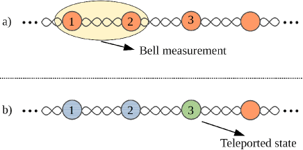
Figure 1: (color online) One run of the teleportation protocol can be essentially divided into four steps, condensed in the two panels above. First, Alice and Bob share an entangled resource (qubits $2$ and $3$) and Alice choose a qubit to be teleported (qubit $1$). Second, Alice implements a Bell measurement (BM) on qubits $1$ and $2$. A BM is a joint measurement on the qubit to be teleported to Bob and on one of the qubits of the entangled state shared with Bob. This step of the protocol is depicted in panel (a) above. Third, Alice informs Bob of her measurement result. There are four possibilities here and she needs to send two classical bits to Bob in order to tell him about which Bell state she measured. Fourth, Bob applies an appropriate unitary operation on his qubit depending on which Bell state Alice measured. After this step, the protocol ends and it is illustrated in panel (b). Bob’s qubit at the end of a run of the protocol is more or less similar to Alice’s original input state according to the quality of the shared entangled state between them (qubits $2$ and $3$).

Initially, the total state describing the three qubits participating in the teleportation protocol is

$$\rho=\rho_{1}\otimes\rho_{23}$$ (1)

and after one run of the protocol Bob’s qubit is pav23 ; rig17

$$\rho_{{}_{B_{j}}}=\frac{U_{j}Tr_{12}[P_{j}\rho P_{j}]U_{j}^{\dagger}}{Q_{j}}.$$ (2)

In Eq. (2), $Tr_{12}$ is the partial trace over Alice’s qubits (spins 1 and 2), $j$ is the Bell measurement (BM) outcome obtained by Alice ($j=\Psi^{\pm},\Phi^{\pm}$), and $P_{j}$ denotes the four projectors associated with the BMs,

$$P_{\Psi^{\pm}} = |\Psi^{\pm}\rangle\langle\Psi^{\pm}|,$$ (3)

$$P_{\Phi^{\pm}} = |\Phi^{\pm}\rangle\langle\Psi^{\pm}|,$$ (4)

where

$$|\Psi^{\pm}\rangle = (|01\rangle\pm|10\rangle)/\sqrt{2},$$ (5)

$$|\Phi^{\pm}\rangle = (|00\rangle\pm|11\rangle)/\sqrt{2}.$$ (6)

The states given by Eqs. (5)-(6) are the four Bell states.

The other two quantities appearing in Eq. (2) are Alice’s probability to obtain a certain Bell state $j$ pav23 ; rig17 ,

$$Q_{j}=Tr[{P_{j}\rho}],$$ (7)

and the unitary correction $U_{j}$ that Bob must apply on his qubit after being informed by Alice of her measurement outcome.

The unitary correction $U_{j}$ that Bob must implement on his qubit after a run of the protocol depends not only on Alice’s measurement result but also on the entangled state $\rho_{23}$ shared with Alice. The sets $S_{k}$ below give the unitary operations that Bob must apply on his qubit if the shared state between Alice and Bob is the Bell state $|k\rangle$ pav23 ; rig17 ,

$$S_{\Phi^{+}}=\{U_{\Phi^{+}},U_{\Phi^{-}},U_{\Psi^{+}},U_{\Psi^{-}}\}=\{\mathbb{1},\sigma^{z},\sigma^{x},\sigma^{z}\sigma^{x}\},$$ (8)

$$S_{\Phi^{-}}=\{U_{\Phi^{+}},U_{\Phi^{-}},U_{\Psi^{+}},U_{\Psi^{-}}\}=\{\sigma^{z},\mathbb{1},\sigma^{z}\sigma^{x},\sigma^{x}\},$$ (9)

$$S_{\Psi^{+}}=\{U_{\Phi^{+}},U_{\Phi^{-}},U_{\Psi^{+}},U_{\Psi^{-}}\}=\{\sigma^{x},\sigma^{z}\sigma^{x},\mathbb{1},\sigma^{z}\},$$ (10)

$$S_{\Psi^{-}}=\{U_{\Phi^{+}},U_{\Phi^{-}},U_{\Psi^{+}},U_{\Psi^{-}}\}=\{\sigma^{z}\sigma^{x},\sigma^{x},\sigma^{z},\mathbb{1}\}.$$ (11)

Note that $\mathbb{1}$ is the identity matrix and $\sigma^{\alpha}$, with $\alpha=x,y,z$, is the standard Pauli matrix nie00 .

The state $\rho_{23}$ shared between Alice and Bob depends on the system’s quantum phase. In one quantum phase $\rho_{23}$ is more similar to one of the four Bell states while in a different quantum phase it is best approximated by another one. Hence, in order to better characterize the QCPs of a spin chain we will use the four sets $S_{k}$ of unitary operations and also determine the set that gives the most efficient teleportation protocol within a quantum phase.

The efficiency of the teleportation protocol is given by how close the output state $\rho_{{}_{B_{j}}}$ is to the input state $\rho_{1}$ at the end of a run of the protocol. Therefore, in order to quantitatively assess that efficiency, we need to choose quantitative measures of the similarity between the teleported state at the end of the protocol and the initial input state with Alice.

In this work we will be dealing with two measures that quantify the similarity between those two states. The first one is the fidelity uhl76 , which is given by nie00

$$F_{j}(S_{k})=F(\rho_{1},\rho_{{}_{B_{j}}})=\left[Tr\sqrt{\sqrt{\rho_{1}}\rho_{{}_{B_{j}}}\sqrt{\rho_{1}}}\right]^{2}.$$ (12)

In the left hand side of Eq. (12) we made it explicit that the fidelity also depends on the set $S_{k}$ of unitary operations that Bob must apply on his qubit. If the teleported state is exactly equal to Alice’s input state, we obtain $F_{j}=1$, and $F_{j}=0$ if those states are orthogonal. Note that in Ref. nie00 the fidelity is defined as $Tr\sqrt{\sqrt{\rho_{1}}\rho_{{}_{B_{j}}}\sqrt{\rho_{1}}}$. Here we take the square of the previous expression to conform with the definition used in our previous works when the input state was a pure state pav23 and with the original work of Uhlmann uhl76 .

After several implementations (runs) of the protocol, the mean fidelity (or efficiency of the protocol) is pav23 ; rig17 ; rig15 ; gor06

$$\overline{F}(S_{k})=\sum_{j=\Psi^{\mp},\Phi^{\mp}}Q_{j}F_{j}(S_{k}).$$ (13)

Similarly to Ref. pav23 , Eq. (13) is the basic building block from which one teleportation based QCP detector is built. In particular, it is defined as the maximum mean fidelity pav23

$$\overline{\mathcal{F}}=\max_{\{S_{k}\}}{\overline{F}(S_{k})}.$$ (14)

As we will show in the next sections, the functional behavior of $\overline{\mathcal{F}}$ and of its first and second order derivatives in terms of the tuning parameter that drives the change in the system’s Hamiltonian is a very useful QCP detector at zero and finite temperatures.

The second measure we will be using in this work to quantify the similarity between two mixed states is the trace distance nie00 ,

$$D_{j}(S_{k})=D(\rho_{1},\rho_{{}_{B_{j}}})=\frac{1}{2}Tr\left|\rho_{1}-\rho_{{}_{B_{j}}}\right|,$$ (15)

where for an operator $A$ we have $|A|=\sqrt{A^{\dagger}A}$. A direct computation for spin-1/2 density matrices gives

$$D_{j}(S_{k})=\frac{1}{2}\sqrt{(\Delta r_{x})^{2}+(\Delta r_{y})^{2}+(\Delta r_{z})^{2}},$$ (16)

where $\Delta r_{\alpha}(t)=Tr(\rho_{1}\sigma^{\alpha})-Tr(\rho_{{}_{B_{j}}}\sigma^{\alpha})$, with $\sigma^{\alpha}$ being a Pauli matrix. Geometrically, the trace distance is half the Euclidean distance between the points on the Bloch sphere associated with the density matrices $\rho_{1}$ and $\rho_{{}_{B_{j}}}$ nie00 . Therefore, when the two states are equal we have $D_{j}=0$ and the more far apart the two states are in the Bloch sphere the greater $D_{j}$. For orthogonal pure states we have $D_{j}=1$, the maximum possible value for the trace distance.

After several runs of the teleportation protocol, the mean trace distance is given by

$$\overline{D}(S_{k})=\sum_{j=\Psi^{\mp},\Phi^{\mp}}Q_{j}D_{j}(S_{k})$$ (17)

and the second QCP point detector is built minimizing $\overline{D}(S_{k})$ over all sets $S_{k}$,

$$\overline{\mathcal{D}}=\min_{\{S_{k}\}}{\overline{D}(S_{k})}.$$ (18)

Similarly to $\overline{\mathcal{F}}$, the behavior of $\overline{\mathcal{D}}$ and of its first and second order derivatives with respect to the Hamiltonian’s driving parameter turns out to be a very robust QCP detector at zero and finite temperatures.

Remark 1: Note that a high value for the fidelity between two states implies a low value for the trace distance and vice-versa. The fidelity measures the similarity between two states; the more similar the states the greater the fidelity. The trace distance, as its name suggests, measures the distance between those two states; the closer the states the lower the value of the trace distance. This is why for the fidelity we implement a maximization operation while for the trace distance we implement a minimization one.

Remark 2: The reason we use in this work the trace distance in addition to the fidelity to assess the efficiency of the teleportation protocol is related to two facts. First, the expressions for the fidelity between two mixed states are too cumbersome and complicated, while the expressions for the trace distance are relatively simpler. Second, the fidelity is less efficient than the trace distance to detect one of the QCPs of the XXZ model (see Sec. III). For the other models and the other QCP of the XXZ model, both quantities are for all practical purposes equivalent.

II.2 Specific settings

All the models we study here (Secs. III and IV) are one dimensional spin-1/2 chains in the thermodynamic limit ($L\rightarrow\infty$) satisfying periodic boundary conditions ($\sigma^{\alpha}_{L+1}=\sigma^{\alpha}_{1}$). Here the subscript implies that $\sigma^{\alpha}_{j}$ acts on the qubit located at the lattice site $j$. Also, all spin chains are assumed to be in equilibrium with a heat bath (thermal reservoir at temperature $T$) and, as such, the density matrix describing the whole chain is given by the canonical ensemble density matrix

$$\varrho=e^{-H/kT}/Z,$$ (19)

with $Z=Tr[e^{-H/kT}]$ being the partition function and $k$ the Boltzmann’s constant. The density matrix describing a pair of nearest neighbor spins, for instance $\rho_{23}$, is obtained tracing out from $\varrho$ all but spins $2$ and $3$. For all the models investigated here we have wer10b ; pav23 ; osb02

$$\rho_{23}=\left(\begin{array}[]{cccc}a&0&0&e\\ 0&b&c&0\\ 0&c&b&0\\ e&0&0&d\\ \end{array}\right),$$ (20)

where

$$a = \frac{1+2\left\langle\sigma^{z}_{2}\right\rangle+\left\langle\sigma_{2}^{z}\sigma_{3}^{z}\right\rangle}{4},$$ (21)

$$b = \frac{1-\left\langle\sigma_{2}^{z}\sigma_{3}^{z}\right\rangle}{4},$$ (22)

$$c = \frac{\left\langle\sigma_{2}^{x}\sigma_{3}^{x}\right\rangle+\left\langle\sigma_{2}^{y}\sigma_{3}^{y}\right\rangle}{4},$$ (23)

$$d = \frac{1-2\left\langle\sigma^{z}_{2}\right\rangle+\left\langle\sigma_{2}^{z}\sigma_{3}^{z}\right\rangle}{4},$$ (24)

$$e = \frac{\left\langle\sigma_{2}^{x}\sigma_{3}^{x}\right\rangle-\left\langle\sigma_{2}^{y}\sigma_{3}^{y}\right\rangle}{4}.$$ (25)

For the XXZ and XX models $\left\langle\sigma_{2}^{x}\sigma_{3}^{x}\right\rangle=\left\langle\sigma_{2}^{y}\sigma_{3}^{y}\right\rangle$ while for the Ising and XY models $\left\langle\sigma_{2}^{x}\sigma_{3}^{x}\right\rangle\neq\left\langle\sigma_{2}^{y}\sigma_{3}^{y}\right\rangle$. We should also note that the translational invariance of the spin chain implies that $\left\langle\sigma^{\alpha}_{j}\right\rangle=\left\langle\sigma^{\alpha}_{k}\right\rangle$ and $\left\langle\sigma^{\alpha}_{j}\sigma^{\beta}_{j+1}\right\rangle=\left\langle\sigma^{\alpha}_{k}\sigma^{\beta}_{k+1}\right\rangle$, for any value of $j,k$.

The evaluation in the thermodynamic limit and for arbitrary values of $T$ of the one-point and two-point correlation functions,

$$z = \left\langle\sigma_{j}^{z}\right\rangle=Tr[\sigma_{j}^{z}\,\varrho],$$ (26)

$$\alpha\alpha = \left\langle\sigma_{j}^{\alpha}\sigma_{j+1}^{\alpha}\right\rangle=Tr[\sigma_{j}^{\alpha}\sigma_{j+1}^{\alpha}\,\varrho],$$ (27)

where $\alpha=x,y,z$, can be found in Refs. yan66 ; clo66 ; klu92 ; bor05 ; boo08 ; tri10 ; tak99 ; lie61 ; bar70 ; bar71 ; pfe70 ; zho10 . In Ref. wer10b these calculations are reviewed and written in the present notation. The behavior of $\left\langle\sigma_{j}^{z}\right\rangle$ and $\left\langle\sigma_{j}^{\alpha}\sigma_{j+1}^{\alpha}\right\rangle$ for several values of $T$ as we change the tuning parameter for each one of the models given in Secs. III and IV are shown in Ref. pav23 .

The density matrix $\rho_{1}$ describing a single spin is calculated by tracing out from the thermal state $\varrho$ [Eq. (19)] all but one spin. Or, equivalently, by tracing out one of the spins from $\rho_{23}$. Therefore, a simple calculation gives

$$\rho_{1}=\left(\begin{array}[]{cc}\frac{1+\left\langle\sigma^{z}\right\rangle}{2}&0\\ 0&\frac{1-\left\langle\sigma^{z}\right\rangle}{2}\end{array}\right),$$ (28)

where we have dropped the subscript from the one-point correlation function for simplicity.

Inserting Eqs. (1), (3), (4), (20), and (28) into Eq. (7) gives

$$Q_{\Psi^{\pm}} = (1-z^{2})/4,$$ (29)

$$Q_{\Phi^{\pm}} = (1+z^{2})/4,$$ (30)

where $z$ is given by Eq. (26).

Using now Eqs. (12), (29) and (30), the mean fidelity given by Eq. (13) becomes,

$$\overline{F}(S_{\Psi^{\pm}}) = \frac{1}{8}\left(\sqrt{(1+z)f(zz,-z)}+\sqrt{(1-z)f(zz,z)}\right)^{2}+\frac{1}{8}\left(\sqrt{(1-z)g(zz,z)}+\sqrt{(1+z)g(zz,-z)}\right)^{2},$$ (31)

$$\overline{F}(S_{\Phi^{\pm}}) = \frac{1}{8}\left(\sqrt{(1-z)f(zz,-z)}+\sqrt{(1+z)f(zz,z)}\right)^{2}+\frac{1}{8}\left(\sqrt{(1+z)g(zz,z)}+\sqrt{(1-z)g(zz,-z)}\right)^{2},$$ (32)

where

$$f(zz,z) = 1+z+z^{2}+z\cdot zz,$$ (33)

$$g(zz,z) = 1-z-z^{2}+z\cdot zz.$$ (34)

Note that the dot between $z$ and $zz$ in Eqs. (33) and (34) means the standard multiplication between the one-point correlation function $z$ and the two-point correlation function $zz$, Eqs. (26) and (27) respectively.

As anticipated in the second remark at the end of Sec. II.1, the expressions for the fidelities are not simple and the maximum mean fidelity becomes

$$\overline{\mathcal{F}}=\max{\left[\,\overline{F}(S_{\Psi^{\pm}}),\overline{F}(S_{\Phi^{\pm}})\right]},$$ (35)

with $\overline{F}(S_{\Psi^{\pm}})$ and $\overline{F}(S_{\Phi^{\pm}})$ given by Eqs. (31) and (32).

Equation (35) is the first teleportation based QCP detector we will be using in this work. The second one is based on the trace distance.

If we repeat the above calculation using Eqs. (16), (29) and (30), the mean trace distance given by Eq. (17) becomes,

$$\overline{D}(S_{\Psi^{\pm}}) = \frac{1}{4}\left[(2+z^{2}+zz)|z|+|z^{3}-z\cdot zz|\right],$$ (36)

$$\overline{D}(S_{\Phi^{\pm}}) = \frac{1}{4}\left[(2-z^{2}-zz)|z|+|z^{3}-z\cdot zz|\right],$$ (37)

and the minimum mean trace distance is according to Eq. (18) given by

$$\overline{\mathcal{D}} = \min{\left[\,\overline{D}(S_{\Psi^{\pm}}),\overline{D}(S_{\Phi^{\pm}})\right]}$$ (38)

$$= \frac{1}{4}\left[(2-|z^{2}+zz|)|z|+|z^{3}-z\cdot zz|\right].$$

Equation (38) is our second teleportation based QCP detector. In Secs. III and IV we investigate the effectiveness of both QCP detectors, Eqs. (35) and (38), in spotlighting the correct location of the QCP for several models at zero and non-zero temperatures.

Remark 3: Equations (35) and (38) do not depend on the two-point correlation functions $xx=\left\langle\sigma_{j}^{x}\sigma_{j+1}^{x}\right\rangle$ and $yy=\left\langle\sigma_{j}^{y}\sigma_{j+1}^{y}\right\rangle$, as can be seen looking at Eqs. (31), (32), (36), and (37). The underlying reason for this is the specific form of $\rho_{1}$ [Eq. (28)]. Whenever the input state to be teleported is diagonal in the standard basis $\{|0\rangle,|1\rangle\}$, the expressions for the fidelity and for the trace distance will not depend on $xx$ and $yy$ if $\rho_{23}$ is given by Eq. (20). For input states having non-diagonal terms, though, a direct calculation shows that both the fidelity and the trace distance will also depend on $xx$ and $yy$.

Remark 4: Contrary to the scenario in which the qubit to be teleported is external to the spin chain pav23 , the expressions for the fidelity and for the trace distance now depend on the one-point correlation function $z=\left\langle\sigma_{j}^{z}\right\rangle$. This happens because in the present case (internal teleportation), the input state to be teleported is a function of $z$, as can be seen looking at Eq. (28). And this implies that the teleported states with Bob are, according to Eq. (2),

$$\rho_{{}_{B_{\Psi^{\pm}}}}(S_{\Psi^{\pm}}) = \frac{1}{2(1-z^{2})}\left(\begin{array}[]{cc}g(zz,-z)&0\\ 0&g(zz,z)\end{array}\right),$$ (41)

$$\rho_{{}_{B_{\Phi^{\pm}}}}(S_{\Psi^{\pm}}) = \frac{1}{2(1+z^{2})}\left(\begin{array}[]{cc}f(zz,-z)&0\\ 0&f(zz,z)\end{array}\right),$$ (44)

$$\rho_{{}_{B_{\Psi^{\pm}}}}(S_{\Phi^{\pm}}) = \frac{1}{2(1-z^{2})}\left(\begin{array}[]{cc}g(zz,z)&0\\ 0&g(zz,-z)\end{array}\right),$$ (47)

$$\rho_{{}_{B_{\Phi^{\pm}}}}(S_{\Phi^{\pm}}) = \frac{1}{2(1+z^{2})}\left(\begin{array}[]{cc}f(zz,z)&0\\ 0&f(zz,-z)\end{array}\right),$$ (50)

where $f(zz,z)$ and $g(zz,z)$ are given by Eqs. (33) and (34), respectively. In Eqs. (41)-(50) we have explicitly written the dependence of Bob’s final state on the set $S_{k}$ containing the unitary corrections that he can implement on his qubit. In other words, $\rho_{{}_{B_{j}}}(S_{k})$ denotes the final state with Bob if Alice measures the Bell state $j$ and Bob corrects his qubit using the corresponding unitary correction listed in $S_{k}$ [cf. Eqs. (8)-(11)].

Remark 5: If we set $z=0$, Eqs. (31), (32), (36), and (37) become $\overline{F}(S_{\Psi^{\pm}})=\overline{F}(S_{\Phi^{\pm}})=1$ and $\overline{D}(S_{\Psi^{\pm}})=\overline{D}(S_{\Phi^{\pm}})=0$. This means that the present method to detect QCPs does not work for the classes of spin chains studied here that do not have a net magnetization. For instance, it does not work for the XXZ model when the external magnetic field is zero since in this case we always have $z=0$ as we drive the system across its QCPs wer10b ; pav23 . In other words, whenever $z=0$ the output state with Bob at the end of the teleportation protocol will always be exactly equal to the input state of Alice regardless of the quantum phase of the system. We will always obtain the same constant values for the maximum mean fidelity ($\overline{\mathcal{F}}=1$) and for the minimum mean trace distance ($\overline{\mathcal{D}}=0$) in all quantum phases.

III The XXZ model in an external field

The XXZ spin chain in an external longitudinal magnetic field is described by the following Hamiltonian, where we set $\hbar=1$,

$$H=\sum_{j=1}^{L}\left(\sigma^{x}_{j}\sigma^{x}_{j+1}+\sigma^{y}_{j}\sigma^{y}_{j+1}+\Delta\sigma^{z}_{j}\sigma^{z}_{j+1}-\frac{h}{2}\sigma^{z}_{j}\right).$$ (51)

In Eq. (51) $\Delta$ is the tuning parameter and $h$ is the external field.

The XXZ model has two QCPs at zero temperature yan66 ; clo66 ; klu92 ; bor05 ; boo08 ; tri10 ; tak99 . For a given field $h$, as we vary $\Delta$ we see at $\Delta=\Delta_{1}$ the first QPT, with the system’s ground state changing from a ferromagnetic ($\Delta<\Delta_{1}$) to a critical antiferromagnetic phase ($\Delta_{1}<\Delta<\Delta_{2}$). If we continue to increase $\Delta$, we have at $\Delta=\Delta_{2}$ another QPT, where the spin chain becomes an Ising-like antiferromagnet.

The value of $\Delta_{1}$ as a function of $h$ is given by the solution of

$$h=4J(1+\Delta_{1}).$$ (52)

On the other hand, $\Delta_{2}$ is obtained by solving the following equation,

$$h=4\sinh(\eta)\sum_{j=-\infty}^{\infty}\frac{(-1)^{j}}{\cosh(j\eta)},$$ (53)

with $\eta=\cosh^{-1}(\Delta_{2})$. For $h=12$, the value of $h$ adopted in this work, the two critical points are

$$\Delta_{1} = 2.000,$$ (54)

$$\Delta_{2} = 4.875,$$ (55)

with the latter QCP correct within a numerical error of $\pm 0.001$.

Let us start studying the efficacy of the maximum mean fidelity in detecting the two QCPs for the XXZ model in an external field. In Fig. 2 we show $\overline{\mathcal{F}}$ as a function of $\Delta$ for $h=12$ and several values of $T$.

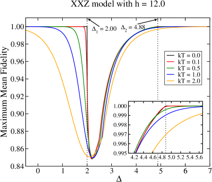
Figure 2: (color online) $\overline{\mathcal{F}}$, Eq. (35), as a function of $\Delta$ for $h=12.0$. At $T=0$ both QCPs are detected by a discontinuity in the derivative of $\overline{\mathcal{F}}$ with respect to $\Delta$. See the inset for a better appreciation of this fact at the second QCP. For $T>0$, these discontinuities in the derivatives are smoothed out and manifest themselves in high values for the magnitudes of the derivatives around the critical points. The dotted lines mark the QCPs and for the solid curves the temperature increases from top to bottom when $\Delta<\Delta_{1}$. Here and in all other graphs all quantities are dimensionless.

Looking at Fig. 2, we realize that $\overline{\mathcal{F}}$ clearly detects the first QCP, with an efficacy compatible to the one we have when employing the external teleportation approach of Ref. pav23 . The detection of the second QCP, though, is not good enough. As we see in the inset of Fig. 2, we need to know the fidelity within an accuracy of $0.001$ to observe a discontinuity in its derivative. And as we increase $T$, we rapidly lose any means of tracking the correct location of the second QCP.

This problem is solved working with the trace distance. In Fig. 3 we show $\overline{\mathcal{D}}$ as a function of $\Delta$ for $h=12$ and the same values of $kT$ given in Fig. 2.

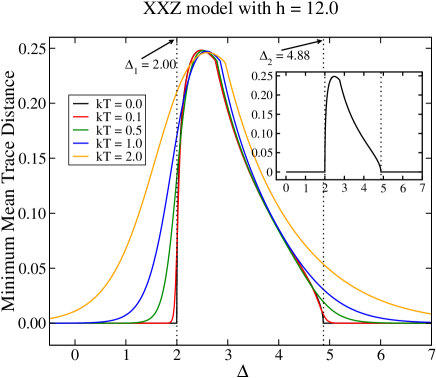
Figure 3: (color online) $\overline{\mathcal{D}}$, Eq. (38), as a function of $\Delta$ for $h=12.0$. Note that now at $T=0$ (see inset) both QCPs are clearly detected by a discontinuity in the derivative of $\overline{\mathcal{D}}$ with respect to $\Delta$. For $T>0$, there are no longer discontinuities in the derivatives. In this case we have high values for the derivatives about the location of the discontinuities that occurred at $T=0$. For $kT\lesssim 0.5$, the extrema of the derivatives lie close together and by extrapolating to $kT\rightarrow 0$ we can correctly determine the QCPs. The dotted lines mark the exact locations of the QCPs and for the solid curves the temperature increases from bottom to top when $\Delta<\Delta_{1}$ and $\Delta>\Delta_{2}$.

Looking at Fig. 3 we note that the two QCPs ($\Delta_{1}$ and $\Delta_{2}$) are clearly detected by discontinuities in the derivatives of $\overline{\mathcal{D}}$ with respect to $\Delta$ as we go through the critical points. Also, in contrast to the behavior of $\overline{\mathcal{F}}$ in the external teleportation approach pav23 , we do not see two extra discontinuities in the derivatives of $\overline{\mathcal{F}}$ and of $\overline{\mathcal{D}}$ [cf. Figs. 2 and 3 with the corresponding ones given in Ref. pav23 ]. In the present case, we only have one small kink between the two QCPs.

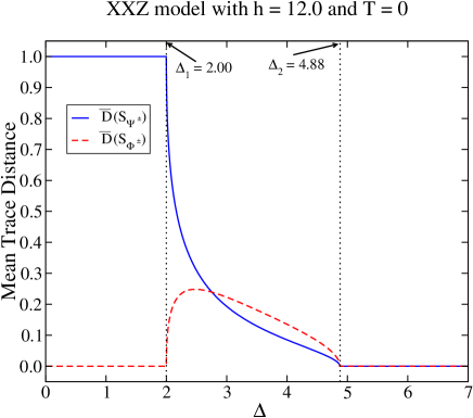
Figure 4: (color online) $\overline{D}(S_{k})$, Eqs. (36) and (37), as a function of $\Delta$ when $T=0$ and $h=12.0$.

This extra kink is related to the exchange of the functions maximizing $\overline{\mathcal{F}}$ or minimizing $\overline{\mathcal{D}}$ as we reach the location of that extra kink. In Fig. 4 we illustrate this point showing at $T=0$ the two expressions appearing in the definition of $\overline{\mathcal{D}}$, Eqs. (36) and (37), as functions of $\Delta$. Before the extra kink the expression minimizing $\overline{\mathcal{D}}$ is given by $\overline{D}(S_{\Phi^{\pm}})$ and after it we have $\overline{D}(S_{\Psi^{\pm}})$. The point where $\overline{D}(S_{\Phi^{\pm}})$ and $\overline{D}(S_{\Psi^{\pm}})$ intersect each other is exactly the point where we see the extra kink in the curve of $\overline{\mathcal{D}}$. Note also that the location of this extra kink changes as we increase the temperature and that the same analysis applies to the fidelity and to higher temperatures as well.

To estimate the values of the two QCPs using finite $T$ data, we employ the same techniques of Refs. wer10b ; pav23 . For finite $T$, the $T=0$ discontinuities in the derivatives of $\overline{\mathcal{D}}$ with respect to $\Delta$ at the QCPs manifest themselves in high values for the magnitudes of these derivatives around the QCPs. The location of these extremum values around the QCPs for several values of $T$ are the key finite $T$ data we need to obtain the QCPs. We can predict the values of the two QCPs by extrapolating to $T=0$ how the locations of those extremum values change as we decrease the temperature.

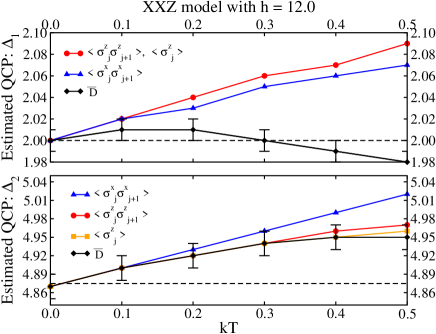
Figure 5: (color online) Estimated QCPs after determining the spots of the extrema of the first order (upper panel) and of the second order (lower panel) derivatives with respect to $\Delta$ for $\overline{\mathcal{D}},\langle\sigma^{x}_{j}\sigma^{x}_{j+1}\rangle,\langle\sigma^{z}_{j}\sigma^{z}_{j+1}\rangle$, and $\langle\sigma^{z}_{j}\rangle$ at several different values of $T$. The dashed lines mark the exact values of the QCPs. The error bars in the curves showing the locations of the extrema of the derivatives of $\overline{\mathcal{D}}$ represent the numerical uncertainty in determining their exact location. For the other quantities in the two panels, similar error bars (not shown) exist about the dots showing the locations of the extrema of their derivatives. See text for details.

Specifically, for six different temperatures, namely, $kT=0,0.1,0.2,0.3,0.4$, and $0.5$, we calculated around the two critical points the values of the one- and two-point correlation functions and of $\overline{\mathcal{D}}$ as a function of $\Delta$. We changed $\Delta$ in increments of $0.01$. Afterwards, we numerically evaluated the first order derivatives of those quantities about $\Delta_{1}$ and their second order derivatives about $\Delta_{2}$. The highest values for the magnitudes of those derivatives can be seen in Fig. 5. Moreover, taking into account that $\Delta$ was changed in increments of $0.01$, the location of the maxima of the magnitudes of the first order derivatives are obtained with an error of $\pm 0.01$. On the other hand, the second order derivatives are calculated from the first order ones, which already possess an error of $\pm 0.01$. Therefore, we estimate that the error of the correct spot for the extremum values of the second order derivatives are no less than $\pm 0.02$. To not clutter the visualization of the other curves, in Fig. 5 we draw error bars depicting these uncertainties only for $\overline{\mathcal{D}}$.

Looking at Fig. 5, we note that for all temperatures the extremum of the first order derivative of $\overline{\mathcal{D}}$ gives the best approximation for the exact value of the first QCP (upper panel of Fig. 5). The second QCP is also better approximated by the the extremum of the second order derivative of $\overline{\mathcal{D}}$ (lower panel of Fig. 5). However, as we decrease $kT$ the other quantities shown in Fig. 5 catch up. Around $kT=0.1$ they are all equally efficient in estimating the location of the second QCP. Also, remembering that for the external teleportation strategy the behavior of the derivatives of $\overline{\mathcal{F}}$ are equal to the behavior of the derivatives of $\langle\sigma^{z}_{j}\sigma^{z}_{j+1}\rangle$ pav23 , we have that the internal teleportation strategy gives better estimates for the location of the two QCPs when compared with the external teleportation approach.

Excluding the $kT=0$ point, we can implement linear and quadratic regressions to find the best curves fitting the remaining data ($kT=0.1,0.2,0.3,0.4,0.5$) pav23 . For all quantities given in the lower panel of Fig. 5, a linear regression is enough to predict the correct location of the QCP $\Delta_{2}$ as we take the $T=0$ limit. The predicted location of $\Delta_{2}$ is given within an accuracy of $\pm 0.02$, the estimated numerical error for the location of the extrema of the second order derivatives of all the quantities given in Fig. 5. The same conclusion applies for all but one of the curves given in the upper panel of Fig. 5, where again the fitted straight lines give the correct location of the QCP $\Delta_{1}$ within an accuracy of $\pm 0.01$, the numerical error for the locations of the extrema of the first order derivatives of all the quantities given in Fig. 5. To achieve this same level of accuracy for $\overline{\mathcal{D}}$, though, we need a quadratic regression.

Remark 6: Although the results reported in this section were obtained assuming that the external magnetic field was $h=12$, similar results are obtained for other values of the field.

Remark 7: Instead of using $\overline{\mathcal{D}}$ [Eq. (38)] and its derivatives to estimate the QCPs using finite $T$ data, we could have worked directly with either $\overline{D}(S_{\Phi^{\pm}})$ or $\overline{D}(S_{\Psi^{\pm}})$ [Eqs. (36) or (37)] and their derivatives. All three quantities give similar results in predicting the location of the QCPs.

IV The XY and the Ising model

A spin-1/2 chain in an external transverse magnetic field described by the XY model is given by the following Hamiltonian lie61 ; bar70 ; bar71 ,

$$H\!=\!-\frac{\lambda}{4}\!\sum_{j=1}^{L}\!\left[(1+\gamma)\sigma^{x}_{j}\sigma^{x}_{j+1}+(1-\gamma)\sigma^{y}_{j}\sigma^{y}_{j+1}\right]\!-\frac{1}{2}\!\sum_{j=1}^{L}\!\sigma^{z}_{j}.$$ (56)

In Eq. (56) $\lambda$ is associated with the inverse of the strength of the magnetic field and $\gamma$ is the anisotropy parameter. We obtain the Ising transverse model from Eq. (56) by setting $\gamma=\pm 1$. And if $\gamma=0$ we have the XX model in a transverse magnetic field.

The tuning parameter for the present model can be either $\lambda$ or $\gamma$. Fixing $\gamma$, we have that for $\lambda<1$ the system is in a ferromagnetic ordered phase and as we increase $\lambda$ we reach the QCP $\lambda_{c}=1.0$, where the Ising transition occurs. For $\lambda>1$ the system now lies in a quantum paramagnetic phase pfe70 . There is another QPT for this model when $\lambda>1$ if we change the anisotropy parameter $\gamma$ instead of $\lambda$. This “anisotropy transition” occurs at $\gamma_{c}=0$ lie61 ; bar70 ; bar71 ; zho10 , where the critical point $\gamma_{c}$ separates a ferromagnet ordered phase in the $x$-direction from a ferromagnet ordered phase in the $y$-direction.

IV.1 The $\lambda$ transition

In Figs. 6, 7, and 8 we plot the maximum mean fidelity $\overline{\mathcal{F}}$ as a function of $\lambda$ for three values of $\gamma$ and for several values of temperature. The chosen values for $\gamma$ are such that we obtain the isotropic XX model ($\gamma=0.0$), the anisotropic XY model ($\gamma=0.5$), and the Ising model ($\gamma=1.0$).

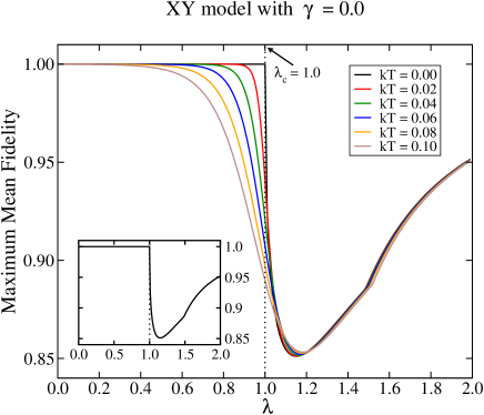
Figure 6: (color online) $\overline{\mathcal{F}}$, Eq. (35), as a function of $\lambda$ and for several values of $kT$ when we fix $\gamma=0.0$ (XX model in a transverse field) [see Eq. (56)]. The inset highlights the $T=0$ curve. The dotted lines mark the QCP $\lambda_{c}$ and for the solid curves the temperature increases from top to bottom when $\lambda<\lambda_{c}$.

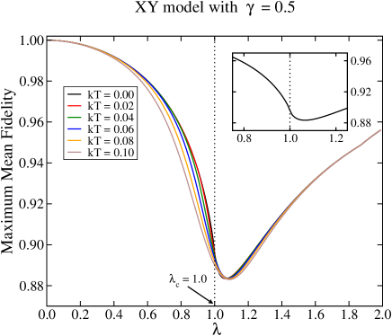
Figure 7: (color online) Same as Fig. 6 but now $\gamma=0.5$.

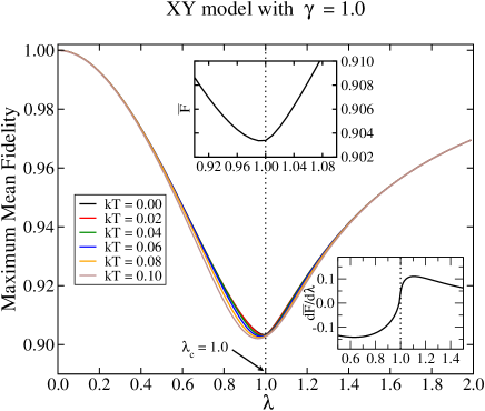
Figure 8: (color online) Same as Fig. 6 but now $\gamma=1.0$ (Ising model in a transverse field). The upper inset highlights the $T=0$ curve of $\overline{\mathcal{F}}$ and the lower inset its derivative with respect to $\lambda$.

For the isotropic XX model ($\gamma=0.0$), the QCP is clearly detect at $T=0$ by a discontinuity in the derivative of $\overline{\mathcal{F}}$ at $\lambda_{c}=1.0$ (see Fig. 6) as well as discontinuities in the derivatives of the one- and two-point correlation functions pav23 . For $T>0$, the discontinuity in the derivative manifests itself in a high value for the derivative’s magnitude about the QCP. The location of the extremum values of the derivatives move away from the QCP as we change $T$. Nevertheless, as we will see for $kT\lesssim 0.1$, these extrema lie close to the correct value of the QCP and we can properly infer the correct location of $\lambda_{c}$ by extrapolating to $kT=0$.

When $\gamma=0.5$ (anisotropic XY model) and $\gamma=1.0$ (Ising transverse model), the QCP is determined, respectively, by the inflection points of $\overline{\mathcal{F}}$ and $d\overline{\mathcal{F}}/d\lambda$ that occur exactly at $\lambda_{c}=1.0$ when $T=0$ (see Figs. 7 and 8). For higher values of $T$, the inflection points are displaced away from $\lambda_{c}$ and the best strategy to estimate the QCP is by determining the location of the maximum (minimum) of the second order derivatives of $\overline{\mathcal{F}}$ with respect to $\lambda$. The location of these extremum values lie close to $\lambda_{c}$ when $kT\lesssim 0.1$ and, as we will show below, by extrapolating to the absolute zero temperature we can predict its correct value. Note also that the one- and two-point correlation functions have inflection points at the QCP when $T=0$ pav23 .

In Figs. 9, 10, and 11 we plot the minimum mean trace distance $\overline{\mathcal{D}}$ as a function of $\lambda$ for the same three values of $\gamma$ and temperatures shown in Figs. 6 to 8. Looking at Figs. 6 to 11, and taking into account that a high value for $\overline{\mathcal{F}}$ implies a low value for $\overline{\mathcal{D}}$, we realize that the behavior of $\overline{\mathcal{F}}$ and $\overline{\mathcal{D}}$ about the QCPs are very similar for a given value of $\gamma$.

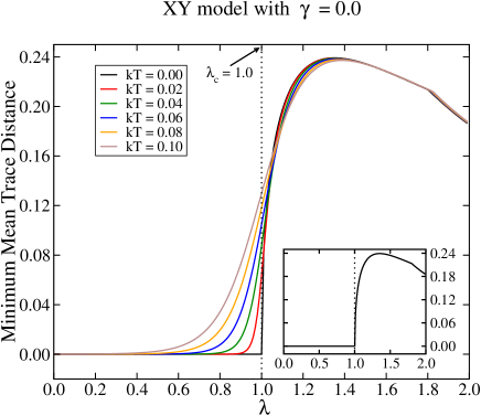
Figure 9: (color online) $\overline{\mathcal{D}}$, Eq. (38), as a function of $\lambda$ for several values of $kT$ while fixing $\gamma=0.0$ (XX model in a transverse field). The inset shows the $T=0$ curve and the dotted lines mark the QCP $\lambda_{c}$. For the solid curves the temperature decreases from top to bottom when $\lambda<\lambda_{c}$.

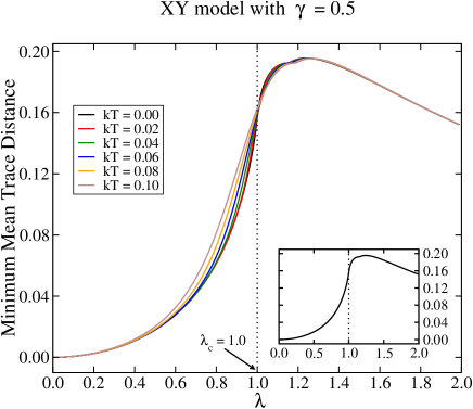
Figure 10: (color online) Same as Fig. 9 but now $\gamma=0.5$.

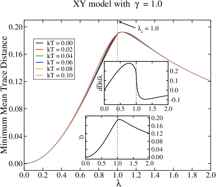
Figure 11: (color online) Same as Fig. 9 but now $\gamma=1.0$ (Ising model in a transverse field). The lower inset highlights the $T=0$ curve of $\overline{\mathcal{D}}$ and the upper inset its derivative with respect to $\lambda$.

Similarly to the behavior of $\overline{\mathcal{F}}$ at $T=0$, for the isotropic XX model ($\gamma=0.0$) the QCP is identified by a discontinuity in the derivative of $\overline{\mathcal{D}}$ with respect to $\lambda$ at $\lambda_{c}$ (see Fig. 9). For $T>0$, we no longer have a discontinuity in the derivative of $\overline{\mathcal{D}}$ but rather a high value for its magnitude about the QCP. The location of this extremum moves away from the exact value of the QCP as we increase $T$. For $kT\lesssim 0.1$, though, these extrema are near to the correct value of the QCP and we will show in what follows how to use these finite $T$ data to extract the exact location of the QCP.

The same qualitative features observed for the behavior of $\overline{\mathcal{F}}$ as a function of $\lambda$ can be seen for $\overline{\mathcal{D}}$ when we work with $\gamma=0.5$ (anisotropic XY model) and $\gamma=1.0$ (Ising transverse model). Again, at $T=0$ the critical point $\lambda_{c}$ is given, respectively, by an inflection point of $\overline{\mathcal{D}}$ and of $d\overline{\mathcal{D}}/d\lambda$ at $\lambda_{c}=1.0$ (see Figs. 10 and 11). If we increase $T$, though, the inflection points move away from $\lambda_{c}=1.0$. As we will see, using finite $T$ data we can best estimate the correct value for $\lambda_{c}$ by computing the location of the extremum values of the second order derivatives of $\overline{\mathcal{D}}$ with respect to $\lambda$ and then numerically taking the $T=0$ limit.

Let us show now how to determine the QCPs using finite $T$ data. Following the strategy outlined in Sec. III, for several values of temperature we numerically evaluate the first and second order derivatives with respect to $\lambda$ of $\overline{\mathcal{D}}$, $\overline{\mathcal{F}}$, and of the one- and two-point correlation functions. Then, we employ the location of the extrema of those derivatives as the value for the QCP. When $\gamma=0.0$, the location of the maximum of the first order derivative of $\overline{\mathcal{D}}$ is the optimal strategy to obtain the correct value for $\lambda_{c}$ (see Fig. 12). Indeed, for all values of temperature up to $kT=0.1$, the predicted value for $\lambda_{c}$ lies within the correct $T=0$ value ($\lambda_{c}=1.0$) if we take into account, as explained in Sec. III, the uncertainties ($\pm 0.01$) in obtaining the spot of the maximum of $d\overline{\mathcal{D}}/d\lambda$.

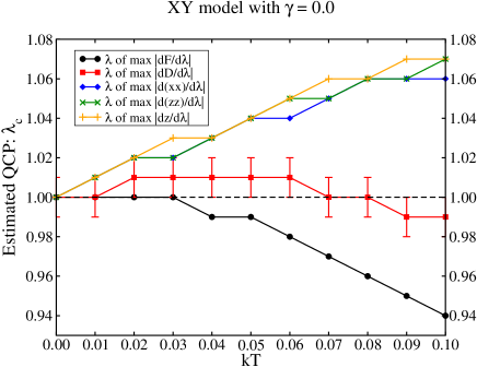
Figure 12: (color online) Estimated value for the critical point $\lambda_{c}$ using finite $T$ data. The locations of the maxima of the first order derivatives of $\overline{\mathcal{D}}$ with respect to $\lambda$ for several values of $T$ best approximate the correct location of the QCP (red-square curve). The error bars depict the uncertainties in numerically obtaining the location of the maxima of $d\overline{\mathcal{D}}/d\lambda$. The dashed line gives the exact value of the QCP and the other solid curves give the locations of the extrema of the first order derivatives of $\overline{\mathcal{F}}$ and of the one- and two-point correlation functions. For ease of visualization, we do not show the error bars in these cases. See text for details.

If we now fix $\gamma=0.5$, the extrema of $d^{2}\overline{\mathcal{F}}/d\lambda^{2}$ lie closer to the true value of the QCP than those of $d^{2}\overline{\mathcal{D}}/d\lambda^{2}$ when $kT>0.02$ (see Fig. 13). For high values of $kT$, the extrema of $d(xx)/d\lambda$ is the optimal choice to estimate the QCP and, as we keep decreasing $T$, all quantities eventually give the exact location for the QCP. It is worth noting that if we take into account the errors (yellow-shaded regions in Fig. 13) in numerically locating the extrema of $d^{2}\overline{\mathcal{F}}/d\lambda^{2}$, for all temperatures shown in Fig. 13 the exact value of the QCP lie within the range of the possible values for the location of those extrema.

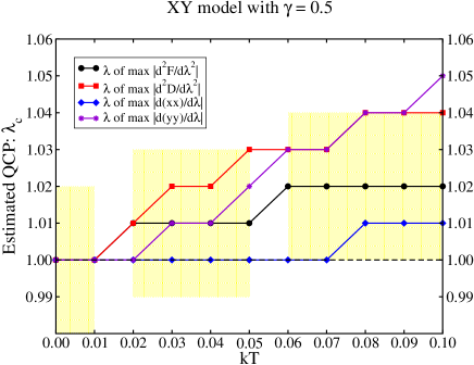
Figure 13: (color online) Same as Fig. 12. The yellow-shaded regions represent the uncertainty in the numerical determination of the locations of the extrema for the second derivatives of $\overline{\mathcal{F}}$ ($\pm 0.02$). For ease of visualization, we do not show the errors associated with the other quantities and we do not show the curves and points giving the locations of the extrema of $dz/d\lambda$ and $d(zz)/d\lambda$. The latter curves lie between the curves above depicting the locations of the extrema for $d(yy)/d\lambda$ and $d(xx)/d\lambda$.

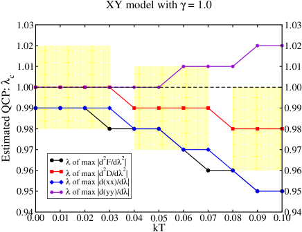
Figure 14: (color online) Same as Fig. 12. The yellow-shaded regions represent the uncertainty in the numerical determination of the locations of the extrema for the second derivatives of $\overline{\mathcal{D}}$ ($\pm 0.02$). For ease of visualization, we do not show the errors associated with the other quantities and we do not show the locations of the extrema of $dz/d\lambda$ and $d(zz)/d\lambda$, which lie between the curves above showing the locations of the extrema for $d(yy)/d\lambda$ and $d(xx)/d\lambda$.

When $\gamma=1.0$, we realize looking at Fig. 14 that up to $kT=0.03$ the extrema of $d(yy)/d\lambda$ and $d^{2}\overline{\mathcal{D}}/d\lambda^{2}$ give the correct value for the QCP. And if we take into account the errors in numerically estimating the extrema of $d^{2}\overline{\mathcal{D}}/d\lambda^{2}$, both quantities are almost equally optimal in predicting the correct value of the QCP for higher values of $kT$ (see Fig. 14).

We can be more quantitative in the prediction of the location of the QCP by following the same strategy of Ref. pav23 that was already explained in Sec. III. For all the quantities shown in Figs. 12 to 14, we excluded the $kT=0.0$ point and implemented a linear regression with the remaining data ($kT=0.01,0.02,\ldots,0.10$). Using the fitted curves, we took the $kT=0$ limit and obtained for all cases and within the numerical errors already reported the correct value for the QCP.

A closer look at the curves for $\overline{\mathcal{D}}$

Before we move to the study of the anisotropy transition, it is important to better analyze the behavior of the minimum mean trace distance $\overline{\mathcal{D}}$ as a function of $\lambda$ (a similar analysis applies to $\overline{\mathcal{F}}$ as well). Looking at Fig. 9, where we fixed $\gamma=0.0$, we note a cusp located about $\lambda=1.8$ that is not associated with a QPT. The origin of this cusp can be traced back to the point where the function minimizing $\overline{\mathcal{D}}$, namely, $\overline{D}(S_{\Phi^{\pm}})$, is replaced by $\overline{D}(S_{\Psi^{\pm}})$. This is illustrated in Fig. 15, where we can also understand the cusp seen at $\lambda\approx 1.5$ for $\overline{\mathcal{F}}$ in Fig. 6. This is the point where $\overline{F}(S_{\Psi^{\pm}})=\overline{F}(S_{\Phi^{\pm}})$. Before this point $\overline{\mathcal{F}}$ is given by $\overline{F}(S_{\Phi^{\pm}})$ and after it by $\overline{F}(S_{\Psi^{\pm}})$.

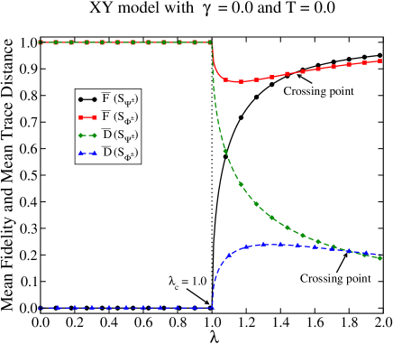
Figure 15: (color online) Mean fidelities $\overline{F}(S_{\Psi^{\pm}})$ and $\overline{F}(S_{\Phi^{\pm}})$ [Eqs. (31) and (32)] and mean trace distances $\overline{D}(S_{\Psi^{\pm}})$ and $\overline{D}(S_{\Phi^{\pm}})$ [Eqs. (36) and (37)] as a function of $\lambda$ when $kT=0$ and $\gamma=0.0$ (XX model in a transverse field). The highlighted points, which we called “crossing points”, are located exactly at the cusps of $\overline{\mathcal{F}}$ and $\overline{\mathcal{D}}$ seen in Figs. 6 and 9, respectively. Note that these cusps are not related to QPTs and they move to higher values of $\lambda$ as we increase the temperature.

Plotting the same curves for $\gamma=0.5$ and $\gamma=1.0$, we realize that the mean fidelity curves as well as the mean trace distance ones do not cross each other. This is why we do not have a cusp in Figs. 7 and 8 and also in Fig. 11. We do have a small cusp, though, for the curves of $\overline{\mathcal{D}}$ given in Fig. 10, where we fixed $\gamma=0.5$. This cusp is not related to a QPT and we can understand its origin by carefully looking at the functional form of $\overline{D}(S_{\Phi^{\pm}})$, which gives the minimum mean trace distance $\overline{\mathcal{D}}$ when $0\leq\lambda\leq 2$ (see Fig. 16).

Looking at Eq. (37), we note that the second term defining $\overline{D}(S_{\Phi^{\pm}})$ is $|z^{3}-z\cdot zz|$. Studying the sign of $z^{3}-z\cdot zz$, we realize that before the cusp seen in Fig. 10 we have $z^{3}-z\cdot zz<0$ while after it we have $z^{3}-z\cdot zz>0$. The change of sign of $z^{3}-z\cdot zz$ leads to a discontinuity in the derivative of $\overline{D}(S_{\Phi^{\pm}})$ with respect to $\lambda$ and this gives rise to the cusp seen in Fig. 10. When $\gamma=1.0$, however, we have $z^{3}-z\cdot zz\leq 0$ when $0.0\leq\lambda\leq 2.0$ and this is why we do not see a similar cusp in Fig. 11.

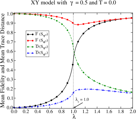
Figure 16: (color online) Same as Fig. 15 but now we have $\gamma=0.5$ (anisotropic XY model in a transverse field). Note that the solid curves do not cross each other. The same applies to the dashed ones.

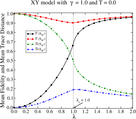
Figure 17: (color online) Same as Fig. 16 but now we have $\gamma=1.0$ (Ising transverse model).

Studying the behavior of $z^{3}-z\cdot zz$ and of $z$, specifically their sign for $0.0\leq\lambda\leq 2.0$, we can simplify the expressions for $\overline{\mathcal{D}}$ within that range of values for $\lambda$. When $\gamma=0$, we have $z^{3}-z\cdot zz\geq 0$ and $z>0$ pav23 . Thus, Eq. (38) becomes

$$\overline{\mathcal{D}}_{\gamma=0}=\left\{\begin{array}[]{ccc}z(1-zz)/2,&\mbox{if}&zz\geq-z^{2},\\ z(1+z^{2})/2,&\mbox{if}&zz\leq-z^{2}.\end{array}\right.$$ (57)

Note that the condition $zz=-z^{2}$ is the solution to $\overline{D}(S_{\Phi^{\pm}})=\overline{D}(S_{\Psi^{\pm}})$, which determines one of the crossing points shown in Fig. 15.

If we now set $\gamma=0.5$, we have that $\overline{\mathcal{D}}$ is always given by $\overline{D}(S_{\Phi^{\pm}})$ (cf. Fig. 16). We also have for $0.0\leq\lambda\leq 2.0$ that $z>0$ pav23 . Noting that in this scenario $z^{3}-z\cdot zz$ changes sign at $zz=z^{2}$, we obtain for Eq. (38),

$$\overline{\mathcal{D}}_{\gamma=0.5}=\left\{\begin{array}[]{ccc}z(1-z^{2})/2,&\mbox{if}&zz\geq z^{2},\\ z(1-zz)/2,&\mbox{if}&zz\leq z^{2}.\end{array}\right.$$ (58)

When $\gamma=1.0$ and $0.0\leq\lambda\leq 2.0$, we also have $z>0$ pav23 and $\overline{\mathcal{D}}$ given by $\overline{D}(S_{\Phi^{\pm}})$ (cf. Fig. 17). In this case, though, we always get that $z^{3}-z\cdot zz\leq 0$. Therefore,

$$\overline{\mathcal{D}}_{\gamma=1.0}=z(1-z^{2})/2.$$ (59)

IV.2 The $\gamma$ transition

In Figs. 18 and 19 we plot, respectively, $\overline{\mathcal{F}}$ and $\overline{\mathcal{D}}$ as functions of $\gamma$ while fixing $\lambda=1.5$.

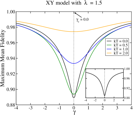
Figure 18: (color online) $\overline{\mathcal{F}}$, Eq. (35), as a function of $\gamma$ with $\lambda=1.5$ [see Eq. (56)]. At $T=0$ (see inset) and $T>0$, the QCP $\gamma_{c}=0.0$ is detected by a minimum that occurs at the exact location of the QCP. The dotted lines spotlight the QCP $\gamma_{c}$ and for the solid curves the temperature increases from bottom to top along the dashed line.

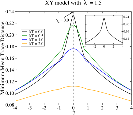
Figure 19: (color online) Same as Fig. 18 but now we have $\overline{\mathcal{D}}$, Eq. (38), as a function of $\gamma$. In this case the QCP is detected by a cusp at $T=0$ (see inset), with the latter being smoothed out as we increase $kT$. For the solid curves, the temperature increases from top to bottom along the dashed line.

Looking at Fig. 18, we note that the QCP located at $\gamma_{c}=0.0$ is given by the global minimum of $\overline{\mathcal{F}}$, which occur exactly at $\gamma_{c}$ even for finite $T$. If we now look at Fig. 19, we realize that the global maximum of $\overline{\mathcal{D}}$ marks the location of the QCP. At $T=0$ we also have a cusp at the maximum, which is smoothed out as we increase $T$. However, the maximum of $\overline{\mathcal{D}}$ is not displaced as we increase $T$, being always situated at the exact location of the QCP. There are two other cusps in the curve for $\overline{\mathcal{D}}$ that are not related to QPTs. They occur when $z^{3}-z\cdot zz$ changes sign. Before the first cusp and after the last cusp we have $z^{3}-z\cdot zz<0$ while between those cusps we have $z^{3}-z\cdot zz>0$. Since $\overline{\mathcal{D}}$ depends on the magnitude of $z^{3}-z\cdot zz$, these sign changes lead to two discontinuities of $d\overline{\mathcal{D}}/d\gamma$ as we vary $\gamma$. These discontinuities in the derivatives of $\overline{\mathcal{D}}$ manifest themselves as two cusps in the curves for $\overline{\mathcal{D}}$ that are not related to QPTs.

The robustness of $\overline{\mathcal{D}}$ to spotlight the anisotropy transition as we increase $T$ can be understood by noting three things that are simultaneously true in the neighborhood of the QCP for all the values of temperature shown in Fig. 19. By the neighborhood of the QCP we mean the region between the two cusps depicted in Fig. 19 that are not related to QPTs.

First, in the neighborhood of the QCP we have that $\overline{\mathcal{D}}=\overline{D}(S_{\Phi^{\pm}})$. Second, $z>0$ and $z^{3}-z\cdot zz\geq 0$. Third, $z$ has a maximum at $\gamma_{c}$ while $zz$ has a minimum there pav23 . The first two facts imply that

$$\overline{\mathcal{D}}_{\lambda=1.5}=z(1-zz)/2, zz\leq z^{2}.$$ if (60)

The third fact gives $\dot{z}=\dot{zz}=0$, $\ddot{z}<0$, and $\ddot{zz}>0$ at $\gamma_{c}$, where the single and double dots denote the first and second order derivatives with respect to $\gamma$. A simple calculation using Eq. (60) and the derivatives above give at $\gamma_{c}$,

$$\frac{d}{d\gamma}\overline{\mathcal{D}}_{\lambda=1.5}(\gamma_{c}) = 0,$$ (61)

$$\frac{d^{2}}{d\gamma^{2}}\overline{\mathcal{D}}_{\lambda=1.5}(\gamma_{c}) = \frac{\ddot{z}(1-zz)-z\cdot\ddot{zz}}{2}<0,$$ (62)

where the last inequality comes from the fact that $\ddot{z}<0$, $|zz|\leq 1$, $z>0$, and $\ddot{zz}>0$. In other words, $\overline{\mathcal{D}}$ has always a maximum at the QCP for all the values of temperature given in Fig. 19.

Remark 8: A similar analysis explains why the maximum mean fidelity $\overline{\mathcal{F}}$ has a minimum at the QCP for all the temperatures shown in Fig. 18.

V Discussion

The strategy developed in this work to detect quantum critical points (QCPs) using finite temperature data simplifies the teleportation based QCP detectors first given in Ref. pav23 . In Ref. pav23 , the state to be teleported to one of the qubits of the spin chain was external to it. Here, however, we showed that by using an internal qubit, i.e., a qubit that belongs to the chain itself, we can still detect QCPs with finite $T$ data using the same techniques of Ref. pav23 if we have spin chains embedded in an external magnetic field. In this scenario and for all spin chain models studied here, we showed that the efficiency of the teleportation protocol or its derivative change drastically at a QCP.

The present proposal also retains the remarkable features of the former one pav23 . From a theoretical point of view, all we need to calculate the efficiency of the teleportation protocol, quantified by either the maximum mean fidelity $\overline{\mathcal{F}}$ or the minimum mean trace distance $\overline{\mathcal{D}}$, is the state describing two nearest neighbor qubits of the spin chain [Eq. (20)], with the latter assumed to be in equilibrium with a heat bath at temperature $T$. This two-qubit density matrix is theoretically computed tracing out all but these two nearest neighbors from the canonical ensemble density matrix describing the complete chain. Equivalently, if we are able to compute all the one- and two-point correlation functions we can determine the two-qubit density matrix describing a pair of spins since it is completely characterized by these correlation functions.

The standard approach to study quantum phase transitions also makes use of those correlation functions or of quantities that depend on them (the magnetic susceptibility, for instance). The QCPs are detected at $T=0$ by discontinuities in the $n$-th order derivatives of those quantities at the QCPs. Quantum information theory quantities, such as bipartite or multipartite entanglement and quantum discord, are also useful to spotlight QCPs wu04 ; oli06 ; dil08 ; sar08 ; fan14 ; gir14 ; wer10 ; wer10b . These quantities are also functions of the correlation functions of the system, the same ones we need to theoretically apply the present and the method of Ref. pav23 .

As already pointed out in Ref. pav23 , some of the standard quantities used to detect QCPs (magnetization or magnetic susceptibility, for instance) become less effective to correctly identify the QCPs with finite $T$ data wer10b . And some quantum information theory quantities, in particular the entanglement of formation woo98 , are zero at and around the QCPs as we increase $T$. These quantities cannot be employed to spotlight QCPs after a certain temperature threshold wer10b . On the other hand, a specific measure of non-classical correlations between two systems, namely, quantum discord oll01 ; hen01 , is extremely robust to spotlight QCPs at finite $T$ wer10b . The present internal teleportation based tools to detect QCPs as well as the ones of Ref. pav23 share the quantum discord robustness to detect QCPs with finite $T$ data. In addition to that, and contrary to quantum discord, the present tools and the ones of Ref. pav23 do not become computationally intractable if we deal with high spin systems (high dimensional Hilbert spaces) pav23 .

Turning our attention to the experimental aspects of the present proposal, it is clearly simpler than the external teleportation QCP detector tools pav23 . There is no need to bring a qubit outside from the spin chain to implement the present proposal. The input state to be teleported belongs to the chain itself. Also, the present scheme and that of Ref. pav23 have a straightforward experimental interpretation since they are built on the quantum teleportation protocol. Quantum discord, though, has no direct experimental procedure to its determination.

Furthermore, to execute the teleportation protocol, and thus the present proposal, we need to be able to implement Bell state measurements and local unitary operations on the qubits that belong to a spin chain. A Bell state measurement is a joint measurement involving two qubits that aims to project the two qubits onto one of the four Bell states. This measurement can be divided into the following sequence of three steps nie00 . First, we implement a controlled-not (CNOT) gate on the pair of spins we will be measuring, now called control and target qubits. The CNOT is a two-qubit (non-local) gate whose “truth table” in the standard basis is such that it flips the spin of the target qubit if, and only if, the control qubit is given by $|1\rangle$. The standard basis can be, for instance, the eigenstates of the spin operator $\sigma^{z}$. Second, we implement a Hadamard gate on the control qubit of the CNOT gate. This is a single (local) qubit gate whose truth table is $(|0\rangle+(-)|1\rangle)/\sqrt{2}\rightarrow|0\rangle(|1\rangle)$. Third, we measure the two qubits in the standard (computational) basis $\{|00\rangle,|01\rangle,|10\rangle,|11\rangle\}$. Each one of the four previous outcomes in the standard basis implies that we projected the two qubits onto one of the four Bell states nie00 . The Bell measurement is Alice’s job while Bob’s job is to measure his qubit after implementing the appropriate local operation (local gate) as given by Eqs. (8)-(11). All these gates, the ones needed by Alice and Bob, are already being implemented in spin chain-like systems using state of the art techniques ron15 ; bra19 ; xie19 ; noi22 ; xue22 ; mad22 ; xie22 . We believe that in the near future they can be implemented in the sequence described above to execute the teleportation protocol and consequently the present proposal.

For instance, using superconducting qubits to realize a spin chain, it is already possible to experimentally prepare tens of spins simultaneously with coherence times around $100\mu s$. Also, single and two-qubit gates in this platform can be implemented within $10ns$ to $100ns$, leading to the execution of $10^{3}$ to $10^{4}$ gates per coherence time gam17 . We can also implement spin chains experimentally using quantum dots and wells. For quantum wells built with GaAs, at room temperature the relaxation time is of the order of a few nanoseconds ohn99 . And for GaAs quantum dots, the relaxation time for a qubit is about 50 $\mu s$ at $T\approx 20mK$ han03 while for arrays of Ge/Si quantum dots we have a relaxation time of about $10\mu s$ at $T\approx 5K$ zin10 . These facts, together with the fact that in silicon quantum dots at $T\approx 1K$ we can implement single and two-qubit gates in less than $100ns$ pet22 , imply that at low temperatures ($\approx 1K$) and for silicon quantum dots it is possible to execute one hundred or so gates before the spin chain thermalizes. This number of gates is at least one order of magnitude more than what we need to implement the present proposal, where only a few gates (less than ten) is needed at a given run of the teleportation protocol.

Finally, we should also contrast the present proposal with the standard way of studying QPTs from the experimental point of view. In the standard way, we must measure the one- and two-point correlation functions using, for instance, neutron scattering techniques. The non-analytic properties of these one- and two-point correlation functions at the QCP marks a QPT. In the present proposal, we need only to measure one-point correlation functions after “disturbing” the system in a specific way. Indeed, to reconstruct the state describing his qubit after the teleportation protocol (the “disturbance” in the spin chain), Bob only needs one-point correlation functions. Any single qubit density matrix is completely characterized once we know all the one-point correlation functions $\left\langle\sigma^{x}\right\rangle,\left\langle\sigma^{y}\right\rangle$, and $\left\langle\sigma^{z}\right\rangle$ nie00 . And in all the models investigated here, we only need one correlation function, $\left\langle\sigma^{z}\right\rangle$ to be specific. This is true since the qubit with Bob after the teleportation protocol is diagonal in the standard basis [see Eqs. (41)-(50)]. In other words, we are trading the measurement of two-point correlation functions to experimentally determine a QCP for the measurement of only one one-point correlation function after disturbing the system in a very particular way, namely, after applying all the gates associated with the quantum teleportation protocol.

VI Conclusion

We simplified the teleportation based quantum critical point (QCP) detector of Ref. pav23 in a very important way, reducing the technical demands to its possible experimental realization. Instead of using an external qubit from the spin chain as the input state to be teleported to the chain, in this work we employed a qubit within the spin chain itself. Several spin-1/2 chain models in the thermodynamic limit were used to test the efficacy of this new approach in detecting a QCP at zero and non-zero temperatures. We showed that whenever the spin chain is immersed in an external magnetic field, the present “internal” teleportation based QCP detector retains all the remarkable characteristics of the “external” teleportation based QCP detector of Ref. pav23 . In particular, we showed that the present strategy detects the QCPs for the XXZ model in a longitudinal field, the Ising transverse model, the isotropic XX model in a transverse field, and the anisotropic XY model in a transverse field.

The main idea behind the present and the proposal of Ref. pav23 is to use a pair of qubits from the spin chain as the entangled resource shared between Alice and Bob in the implementation of the teleportation protocol. In this work, an internal qubit of the chain, adjacent to the pair of qubits shared between Alice and Bob, is teleported to Bob. Similarly to what we saw in Ref. pav23 , we proved that the efficiency of the teleportation protocol changes considerably as we cross the QCP. In other words, the efficiency of the teleportation protocol depends on the quantum phase in which the spin chain lies. The efficiency of the teleportation protocol in this work was quantified by using both the fidelity and the trace distance between the input and output states, namely, between Alice’s input state and Bob’s final qubit at the end of the teleportation protocol.

For the several models investigated here, we observed that at $T=0$ the maximum mean fidelity $\overline{\mathcal{F}}$ and the minimum mean trace distance $\overline{\mathcal{D}}$ between the teleported and the input states possess a cusp or an inflection point exactly the QCPs. When we increase $T$, these cusps are smoothed out and both the cusps and the inflection points are displaced from the exact locations of the QCPs. At finite temperatures, these cusps and inflection points manifest themselves in a high value for the magnitudes of the first and second order derivatives of $\overline{\mathcal{F}}$ and $\overline{\mathcal{D}}$ around the exact locations of the QCPs. We also showed that for small values of temperature, the extrema of these derivatives lie close together and by taking the zero temperature limit we are able to correctly predict the $T=0$ location of the QCP.

Furthermore, the internal teleportation based QCP detector share the same features of the external one and of the quantum discord, when the latter is also employed as a tool to detect QCPs wer10b . These tools can be used without the knowledge of the order parameter associated with the quantum phase transition being investigated and they are very resilient to the increase of temperature, giving us useful information at finite $T$ that allows us to predict the exact value of the QCP at $T=0$. On top of that, and contrary to the quantum discord, the QCP detectors here developed and in Ref. pav23 have a straightforward experimental meaning and are scalable to high spin systems pav23 .

We want to end this work calling attention to a feature already highlighted in Ref. pav23 and that is also observed here. This feature is related to the fact that for each model investigated in this work we have a distinctive functional form for $\overline{\mathcal{F}}$ and $\overline{\mathcal{D}}$. For some models we have extra cusps for these functions that are not related to a quantum phase transition, for other models the QCP is detected via an inflection point of $\overline{\mathcal{F}}$ and $\overline{\mathcal{D}}$, and for others we have the QCP being detected by discontinuities in their derivatives. Putting it differently, the “fingerprint” of a quantum phase, a quantum phase transition, and the underlying model dictating these phases and transitions are unique. The functional forms of $\overline{\mathcal{F}}$ and $\overline{\mathcal{D}}$ as we drive the system around its phase space are specific for a given model. A systematic study $\overline{\mathcal{F}}$ and $\overline{\mathcal{D}}$ enables the proper detection of the QCP using finite $T$ data and, interestingly, also the discovery of the underlying spin chain model giving rise to those quantum phases and quantum phase transitions.

- (1) S. Sachdev, Quantum Phase Transitions (Cambridge University Press, Cambridge, 1999).
- (2) M. Greiner, O. Mandel, T. Esslinger, T. W. Hänsch, and I. Bloch, Nature (London) 415, 39 (2002).
- (3) V. F. Gantmakher and V. T. Dolgopolov, Phys. Usp. 53, 1 (2010).
- (4) S. Rowley, R. Smith, M. Dean, L. Spalek, M. Sutherland, M. Saxena, P. Alireza, C. Ko, C. Liu, E. Pugh et al., Phys. Status Solidi B 247, 469 (2010).
- (5) L.-A. Wu, M. S. Sarandy, and D. A. Lidar, Phys. Rev. Lett. 93, 250404 (2004).
- (6) T. R. de Oliveira, G. Rigolin, M. C. de Oliveira, and E. Miranda, Phys. Rev. Lett. 97, 170401 (2006); T. R. de Oliveira, G. Rigolin, and M. C. de Oliveira, Phys. Rev. A 73, 010305 (2006); T. R. de Oliveira, G. Rigolin, M. C. de Oliveira, and E. Miranda, Phys. Rev. A 77, 032325(R) (2008).
- (7) R. Dillenschneider, Phys. Rev. B 78, 224413 (2008).
- (8) M. S. Sarandy, Phys. Rev. A 80, 022108 (2009).
- (9) G. Karpat, B. Çakmak, and F. F. Fanchini, Phys. Rev. B 90, 104431 (2014).
- (10) D. Girolami, Phys. Rev. Lett. 113, 170401 (2014).
- (11) M. Hotta, Phys. Lett. A 372, 5671 (2008).
- (12) M. Hotta, J. Phys. Soc. Jpn. 78, 034001 (2009).
- (13) K. Ikeda, Phys. Rev. D 107, L071502 (2023).
- (14) K. Ikeda, Phys. Rev. Appl. 20, 024051 (2023).
- (15) K. Ikeda, AVS Quantum Sci. 5, 035002 (2023).
- (16) K. Ikeda, R. Singh, and R.-J. Slager, e-print arXiv:2310.15936 [quant-ph].
- (17) W. K. Wootters, Phys. Rev. Lett. 80, 2245 (1998).
- (18) T. Werlang and G. Rigolin, Phys. Rev. A 81, 044101 (2010).
- (19) T. Werlang, C. Trippe, G. A. P. Ribeiro, and G. Rigolin, Phys. Rev. Lett. 105, 095702 (2010); T. Werlang, G. A. P. Ribeiro, and G. Rigolin, Phys. Rev. A 83, 062334 (2011); T. Werlang, G. A. P. Ribeiro, and G. Rigolin, Int.J. Mod. Phys. B 27, 1345032 (2013).
- (20) H. Ollivier and W. H. Zurek, Phys. Rev. Lett. 88, 017901 (2001).
- (21) L. Henderson and V. Vedral, J. Phys. A: Math. Gen. 34, 6899 (2001).
- (22) Y. Huang, New J. Phys. 16, 033027 (2014).
- (23) A. L. Malvezzi, G. Karpat, B. Çakmak, F. F. Fanchini, T. Debarba, and R. O. Vianna, Phys. Rev. B 93, 184428 (2016).
- (24) G. A. P. Ribeiro and G. Rigolin, Phys. Rev. A 107, 052420 (2023); G. A. P. Ribeiro and G. Rigolin, Phys. Rev. A 109, 012612 (2024).
- (25) C. H. Bennett, G. Brassard, C. Crepeau, R. Jozsa, A. Peres, and W. K. Wootters, Phys. Rev. Lett. 70, 1895 (1993).
- (26) Y. Yeo, Phys. Rev. A 66, 062312 (2002).
- (27) R. Fortes and G. Rigolin, Phys. Rev. A 96, 022315 (2017).
- (28) R. Fortes and G. Rigolin, Phys. Rev. A 92, 012338 (2015); 93, 062330 (2016).
- (29) M. A. Nielsen and I. L. Chuang, Quantum Computation and Quantum Information (Cambridge University Press, Cambridge, 2000).
- (30) A. Uhlmann, Rep. Math. Phys. 9, 273 (1976).
- (31) G. Gordon and G. Rigolin, Phys. Rev. A 73, 042309 (2006); 73, 062316 (2006); Eur. Phys. J. D 45, 347 (2007).
- (32) T. J. Osborne and M. A. Nielsen, Phys. Rev. A 66, 032110 (2002).
- (33) C. N. Yang and C. P. Yang, Phys. Rev. 147, 303 (1966).
- (34) J. Cloizeaux and M. Gaudin, J. Math. Phys. 7, 1384 (1966).
- (35) A. Klümper, Ann. Phys. 1, 540 (1992); Z. Phys. B 91, 507 (1993).
- (36) M. Bortz and F. Göhmann, Eur. Phys. J. B 46, 399 (2005).
- (37) H. E. Boos, J. Damerau, F. Göhmann, A. Klümper, J. Suzuki, and A. Weiße, J. Stat. Mech. (2008) P08010.
- (38) C. Trippe, F. Göhmann, and A. Klümper, Eur. Phys. J. B 73, 253 (2010).
- (39) M. Takahashi, Thermodynamics of one-dimensional solvable models (Cambridge University Press, Cambridge, 1999).
- (40) E. Lieb, T. Schultz, and D. Mattis, Ann. Phys. 16, 407 (1961).
- (41) E. Barouch, B. M. McCoy, and M. Dresden, Phys. Rev. A 2, 1075 (1970).
- (42) E. Barouch and B. M. McCoy, Phys. Rev. A 3, 786 (1971).
- (43) P. Pfeuty, Ann. Phys. (New York) 57, 79 (1970).
- (44) M. Zhong and P. Tong, J. Phys. A: Math. Theor. 43, 505302 (2010).
- (45) X. Rong, J. Geng, F. Shi, Y. Liu, K. Xu, W. Ma, F. Kong, Z. Jiang, Y. Wu, and J. Du, Nat. Commun. 6, 8748 (2015).
- (46) C. E. Bradley, J. Randall, M. H. Abobeih, R. C. Berrevoets, M. J. Degen, M. A. Bakker, M. Markham, D. J. Twitchen, and T. H. Taminiau, Phys. Rev. X 9, 031045 (2019).
- (47) T. Xie, Z. Zhao, X. Kong, W. Ma, M. Wang, X. Ye, P. Yu, Z. Yang, S. Xu, P. Wang et al., Sci. Adv. 7, eabg9204 (2021).
- (48) A. Noiri, K. Takeda, T. Nakajima, T. Kobayashi, A. Sammak, G. Scappucci, and S. Tarucha, Nature 601, 338 (2022).
- (49) X. Xue, M. Russ, N. Samkharadze, B. Undseth, A. Sammak, G. Scappucci, and L. M. Vandersypen, Nature 601, 343 (2022).
- (50) M. T. Mądzik, S. Asaad, A. Youssry, B. Joecker, K. M. Rudinger, E. Nielsen, K. C. Young, T. J. Proctor, A. D. Baczewski, A. Laucht et al., Nature 601, 348 (2022).
- (51) T. Xie, Z. Zhao, S. Xu, X. Kong, Z. Yang, M. Wang, Y. Wang, F. Shi, and J. Du, e-print arXiv:2212.02831 [quant-ph].
- (52) J. M. Gambetta, J. M. Chow, and M. Steffen, npj Quantum Inf. 3, 2 (2017).
- (53) Y. Ohno, R. Terauchi, T. Adachi, F. Matsukura, and H. Ohno, Phys. Rev. Lett. 83, 4196 (1999).
- (54) R. Hanson, B. Witkamp, L. M. K. Vandersypen, L. H. W. van Beveren, J. M. Elzerman, and L. P. Kouwenhoven, Phys. Rev. Lett. 91, 196802 (2003).
- (55) A. F. Zinovieva, A. V. Dvurechenskii, N. P. Stepina, A. I. Nikiforov, and A. S. Lyubin, Phys. Rev. B 81, 113303 (2010).
- (56) L. Petit, M. Russ, G. H. G. J. Eenink, W. I. L. Lawrie, J. S. Clarke, L. M. K. Vandersypen, and M. Veldhorst, Commun. Mater. 3, 82 (2022).