Spectral CT Two-step and One-step Material Decomposition using Diffusion Posterior Sampling

Abstract

This paper proposes a novel approach to spectral computed tomography (CT) material decomposition that uses the recent advances in generative diffusion models (DMs) for inverse problems. Spectral CT and more particularly photon-counting CT (PCCT) can perform transmission measurements at different energy levels which can be used for material decomposition. It is an ill-posed inverse problem and therefore requires regularization. DMs are a class of generative model that can be used to solve inverse problems via diffusion posterior sampling (DPS). In this paper we adapt DPS for material decomposition in a PCCT setting. We propose two approaches, namely Two-step Diffusion Posterior Sampling (TDPS) and One-step Diffusion Posterior Sampling (ODPS). Early results from an experiment with simulated low-dose PCCT suggest that DPSs have the potential to outperform state-of-the-art model-based iterative reconstruction (MBIR). Moreover, our results indicate that TDPS produces material images with better peak signal-to-noise ratio (PSNR) than images produced with ODPS with similar structural similarity (SSIM).

I Introduction

Spectral computed tomography (CT) and the energy-dependent attenuation allow to reconstruct images of the materials present within the scanned object or patient [1]. It is an ill-posed inverse problem and requires regularization, or prior. Conventional model-based iterative reconstruction (MBIR) techniques typically include two types of approaches, namely two-step and one-step techniques.

On one hand, two-step techniques aim at reconstructing high-quality multi-energy images which are then used for material decomposition. The images can be reconstructed synergistically to leverage the information shared across channels, for example by enforcing structural similarities [2], low-rank [3, 4] or similarities with a reference clean image [5]. Alternatively, the regularizer can also be trained [6, 7, 8] (see [9] for a review).

On the other hand, one-step techniques directly estimate the material images from the raw projection data. This is also achieved with the help of MBIR techniques to minimize the negative log-likelihood which preserves the Poisson statistics. Likewise, these methods are regularized, for example by promoting pixel-wise material separation [10].

Generative models and particularly diffusion models (DMs) have shown promising results for sampling realistic images from a training dataset [11]. More recently, they have been used to solve inverse problems by guiding the sampling scheme [12] or via diffusion posterior sampling (DPS) [13].

In this work, we propose to solve the material decomposition inverse problem by DPS.

We propose two approaches, Two-step Diffusion Posterior Sampling (TDPS), based on our previous work [14], and One-step Diffusion Posterior Sampling (ODPS), for the decomposition of bone and soft tissue materials.

Section II presents our paradigm, starting from the forward model and the two approaches (two-step and one-step) in Section II-A, followed by the description of the two approaches we developed, namely ODPS and TDPS in Section II-B. Section III presents results of two-material decomposition in simulated photon-counting CT (PCCT) with different X-ray photon flux and compares the two methods proposed to other decomposition techniques. Finally, we discuss and conclude our work in Section IV.

II Method

II-A Spectral CT and Material Decomposition

Building on advances on X-ray CT, it is possible to leverage the energy dependence of the linear attenuation coefficient (LAC) in order to reconstruct multiple images of the same scanned object but at different level of energy $E$.

We (temporarily) denote by

$$\bm{X}(E)=[X_{1}(E),X_{2}(E),\dots,X_{J}(E)]\in\mathbb{R}^{J}$$

the energy-dependent attenuation image (random vector) where $J$ is the number of pixels and $X_{j}(E)$ the LAC at pixel $j$ and energy $E$.

For each pixel $j$, $X_{j}$ can be decomposed as a sum over the materials composing the scanned object or patient. Denoting by $Z_{j,n}$ the $n$-th material concentration at pixel location $j$, we have the following material composition

$$X_{j}(E)={} \sum_{n=1}^{N}f_{n}(E)Z_{j,n}$$

$$\triangleq{} \mathcal{F}(\bm{Z}_{j},E)$$ (1)

where $f_{n}(E)$ is the known $n$-th material attenuation function multiplied by the density of the corresponding material, $\bm{Z}_{j}=\{Z_{j,n}\}_{n=1}^{N}\in\mathbb{R}^{N}$ and $N$ is the number of materials. The $\bm{Z}_{j}$’s are regrouped into a material image $\bm{Z}=\{Z_{j}\}_{j=1}^{J}\in\mathbb{R}^{J\cdot N}$, and $\mathcal{F}$ in (1) can be generalized to the entire image as

$$\mathcal{F}(\bm{Z},E)={} \bm{X}(E)$$

$$\triangleq{} \{\mathcal{F}(\bm{Z}_{j},E)\}_{j=1}^{J}\in\mathbb{R}^{J}\,.$$ (2)

We now consider the standard setting of PCCT. The energy spectra of the X-ray beams is discretized into $K$ energy bins of the form $[E_{k},E_{k+1}]$ and we denote by $Y_{i,k}$ the measurement for the energy bin $k$ and along the $i$-th ray, $i=1,\dots,I$. The $Y_{i,k}$’s are random variables with conditional distribution

$$(Y_{i,k}\mid\bm{Z}=\bm{z})\sim{} (Y_{i,k}\mid\bm{X}(\cdot)=\mathcal{F}(\bm{z},\cdot))$$ (3)

$$\sim{} \mathrm{Poisson}\left(\bar{Y}_{i,k}\left(\mathcal{F}(\bm{z},\cdot)\right)\right)$$ (4)

where the mean number of detection $\bar{Y}_{i,k}$ given some energy-dependent image $\bm{x}(E)=\mathcal{F}(\bm{z},E)$ is

$$\bar{Y}_{i,k}\left(\bm{x}\right)\triangleq\int h_{i,k}(E)\cdot\mathrm{e}^{-[\bm{\mathcal{A}}(\bm{x}(E))]_{i}}\,\mathrm{d}E\,,$$ (5)

$\bm{\mathcal{A}}\colon\mathbb{R}^{J}\to\mathbb{R}^{I}$ being the forward CT operator and $h_{i,k}(E)$ being the photon flux for the energy bin $k$. The random variables $Y_{j,k}$ are conditionally independent given $\bm{X}(\cdot)$ (and therefore given $\bm{Z}$). We regroup all measures into one random vector $\bm{Y}=\{Y_{i,k}\}_{i,k=1}^{I,K}\in\mathbb{R}^{I\cdot K}$.

In this work we consider the standard simplified model where the energy-dependent attenuation $\bm{X}(E)$ is “energy-discretized” into $K$ images $\bm{X}_{k}=[X_{1,k},\dots,X_{J,k}]\in\mathbb{R}^{J}$, one for each energy bin $k$, such that $\bm{X}_{k}$ corresponds to an average attenuation image for energy bin $k$, and we redefine $\bm{X}\triangleq\{\bm{X}_{k}\}_{k=1}^{K}\in\mathbb{R}^{J\cdot K}$ as the vector-valued image regrouping the $K$ energy bins. Moreover, we use an energy-discretized version of (1)

$$X_{j,k}={} \sum_{n=1}^{N}f_{n,k}Z_{n,j}$$

$$\triangleq{} \mathcal{F}_{k}(\bm{Z}_{j})$$

and we redefine the operator $\mathcal{F}$, initially defined in (2), as the generalized material decomposition operator over the entire image for all energy bins as

$$\mathcal{F}(\bm{Z})\triangleq\{\mathcal{F}_{k}(\bm{Z})\}_{j,k=1}^{J,K}\in\mathbb{R}^{J\cdot K}\,.$$

Finally, we have the following simplified forward model:

$$(Y_{i,k}\mid\bm{Z}=\bm{z})\sim{} (Y_{i,k}\mid\bm{X}_{k}=\mathcal{F}_{k}(\bm{z}))$$

$$\sim{} \mathrm{Poisson}\left(\bar{Y}_{i,k}\left(\mathcal{F}_{k}(\bm{z})\right)\right)$$ (6)

where for some attenuation image $\bm{x}_{k}$ at bin $k$ the expected number of counts $\bar{Y}_{i,k}$ is given by a simplified version of (5):

$$\bar{Y}_{i,k}\left(\bm{x}_{k}\right)\triangleq\bar{h}_{i,k}\cdot\mathrm{e}^{{-[\bm{\mathcal{A}}(\bm{x}_{k})]_{i}}}$$ (7)

with $\bar{h}_{i,k}=\int h_{i,k}(E)\mathrm{d}E$.

Thus, given an energy-binned measurement $\bm{Y}=\bm{y}\in\mathbb{R}^{I\cdot K}$, maximum a posteriori (MAP) spectral CT material decomposition can be achieved in two ways: (i) the two-step approach, i.e.,

$$\hat{\bm{x}}\in\operatornamewithlimits{arg\,max}_{\bm{x}\in\mathbb{R}^{I\cdot K}}\,p_{\bm{Y}|\bm{X}=\bm{x}}(\bm{y})\cdot p_{\bm{X}}(\bm{x})\quad\text{then solving}\quad\mathcal{F}(\bm{z})=\hat{\bm{x}}$$ (8)

and (ii) the one-step approach, i.e.,

$$\hat{\bm{z}}\in\operatornamewithlimits{arg\,max}_{\bm{z}\in\mathbb{R}^{J\cdot N}}\,p_{\bm{Y}|\bm{Z}=\bm{z}}(\bm{y})\cdot p_{\bm{Z}}(\bm{z})$$ (9)

where $p_{\bm{Y}|\bm{X}=\bm{x}}$ and $p_{\bm{Y}|\bm{Z}=\bm{z}}$ are given by (3) and (4) and $p_{\bm{X}}$ and $p_{\bm{Z}}$ are respectively the prior probability distribution functions (PDFs) of $\bm{X}$ and $\bm{Z}$.

Solving (8) and (9) is usually achieved with the help of MBIR techniques. In the case of the two-step decomposition (8), the pseudo-inverse of $\mathcal{F}$, denoted $\mathcal{F}^{\dagger}$, can be used to obtain $\hat{\bm{z}}=\mathcal{F}^{\dagger}\left(\hat{\bm{x}}\right)$. However, the log-priors $\log p_{\bm{X}}$ and $\log p_{\bm{Z}}$ are in general unknowns and need to be replaced by handcrafted regularizers. Examples of such regularizers for $\bm{x}\in\mathbb{R}^{J\cdot K}$ in the two-step approach (8) include total variation (TV) or total nuclear variation (TNV) [2] to promote structural similarities across channels or with a reference image [5], as well as low-rank regularizers [3, 4]. The regularizers can also be trained, for example with tensor dictionary learning [6], convolutional dictionary learning [7] or U-Nets [8]. Regularizers for material images $\bm{z}\in\mathbb{R}^{J\cdot N}$ can for instance promote neighboring pixels to have similar values while preserving edges [15] or promote pixel-wise material separation [10].

II-B Diffusion Models

Diffusion models [16, 17] are a new state-of-the-art convolutional neural network (CNN)-based generative models. In previous work [14] we proposed a DPS framework to sample the multi-energy image $\bm{X}\in\mathbb{R}^{J\cdot K}$. This method enables sampling images according to the joint PDF of all channels simultaneously, leveraging inter-channel information. Compared to individually sampling each $\bm{X}_{k}$, this approach enhances image quality, thus potentially improving the quality of material images obtained within a two-step framework, namely TDPS. Similarly, DPS can be used in a one-step framework, namely ODPS, to directly sample the material image $\bm{Z}\in\mathbb{R}^{J\cdot N}$ without reconstructing $\bm{X}$.

II-B1 Image Generation

We denote by $\bm{\xi}\in\{\bm{X},\bm{Z}\}$ the random vector which can be either $\bm{X}$ or $\bm{Z}$ depending on which problem we wish to solve (TDPS or ODPS). In the following paragraph we briefly describe diffusion models to sample $\bm{\xi}$ from $p_{\bm{\xi}}$ and then how to leverage such model to sample from $p_{\bm{\xi}|\bm{Y}}$.

Generative models are used to generate new samples from $p_{\bm{\xi}}$ trained from limited training dataset with empirical PDF $p_{\mathrm{data}}$ that approximates $p_{\bm{\xi}}$. DMs have been recently introduced in image processing and have shown promising performances [11]. Song et al. [12] showed that DMs can be viewed as a stochastic differential equation (SDE) framework. The general idea consists in using a diffusion SDE that pushes the initial distribution $p_{0}=p_{\bm{\xi}}$ into a white noise. The “variance preserving” forward SDE is (in the ideal case $\bm{\xi}_{0}\sim p_{\bm{\xi}}$) [16, 12]

$$\mathrm{d}\bm{\xi}_{t}=-\frac{1}{2}\beta(t)\bm{\xi}_{t}\,\mathrm{d}t+\sqrt{\beta(t)}\mathrm{d}\bm{w}_{t}\textrm{~{}for~{}}t\in[0,T]$$

where $\bm{w}_{t}$ is a standard Wiener process. The function $\beta\colon\mathbb{R}\to\mathbb{R}$ is chosen such that $\bm{\xi}_{T}$ approximately follows a standard normal distribution. We assume that for each $t$ in $[0,T]$, $\bm{\xi}_{t}$ follows the PDF $p_{t}$. According to Anderson [18], the corresponding reverse time SDE is

$$\mathrm{d}\bm{\xi}_{t}=\left[-\frac{1}{2}\beta(t)\bm{\xi}_{t}-\frac{1}{2}\beta(t)\nabla(\log p_{t})(\bm{\xi}_{t})\right]\mathrm{d}t+\sqrt{\beta(t)}\mathrm{d}\bm{w}_{t}\,.$$ (10)

The term $\nabla(\log p_{t})(\cdot)$ is called the score function. It is intractable and we use a deep neural network (NN) $\bm{s}_{\bm{\theta}}(\bm{\xi},t)$ parameterized by $\bm{\theta}$ in order to approximate it. Training $\bm{s}_{\bm{\theta}}$ with a mean squared error (MSE) loss could be achieved as

$$\hat{\bm{\theta}}\in\operatornamewithlimits{arg\,min}_{\bm{\theta}}\>\mathbb{E}_{t\sim\mathcal{U}\{0,T\},\bm{\xi}_{t}\sim p_{\xi}}\left[\lVert\bm{s}_{\bm{\theta}}(\bm{\xi}_{t},t)-\nabla(\log p_{t})(\bm{\xi}_{t})\rVert_{2}^{2}\right]\,.$$

However, since $p_{t}$ is unknown, we use the following surrogate optimization problem which leads to the same minimizer [19]:

$$\hat{\bm{\theta}}\in\operatornamewithlimits{arg\,min}_{\bm{\theta}}\>\mathbb{E}_{t,\bm{\xi}_{0}\sim p_{0},\bm{\xi}_{t}|\bm{\xi}_{0}}\left[\lVert\bm{s}_{\bm{\theta}}(\bm{\xi}_{t},t)-\nabla(\log p_{t|0})(\bm{\xi}_{t})\rVert_{2}^{2}\right]\,,$$

where $\bm{\xi}_{t}|\bm{\xi}_{0}\sim p_{t|0}$ and $p_{\mathrm{data}}$ is used instead of $p_{0}$ to compute the expectation. See [12] appendix C for more details on the computation of $p_{t|0}$. In this work we use the denoising diffusion probabilistic model implementation [16] where the NN predicts noise added during the diffusion instead of the score. This is based on Tweedie’s formula, which enables us to establish a connection between both aspects. We then start from white noise and follow (10) from $t=T$ to $t=0$ with the score replaced by $\bm{s}_{\hat{\bm{\theta}}}$ and obtain a realization of $\bm{\xi}\sim p_{\bm{\xi}}=p_{0}$.

II-B2 Solving Inverse Problems

It is possible to leverage the generative capability of a DM to regularize an inverse problem, see for instance [20, 21]. The idea is to condition the reverse SDE (10) on the measurements $\bm{Y}=\bm{y}$. This leads to the conditional score $\nabla(\log p_{t})(\cdot|\bm{y})$ where $p_{t}(\cdot|\bm{y})\triangleq p_{\bm{\xi}_{t}|\bm{Y}=\bm{y}}(\cdot)$, which, thanks to Bayes’ rule can be written as $\nabla(\log p_{t})(\cdot)+\nabla(\log p_{t})(\bm{y}|\cdot)$. The first term is the unconditional score and is approximated with a NN as before. In this work, we use the DPS method [13] and approximate the second term by

$$\nabla_{\bm{\xi}_{t}}(\log p_{t})(\bm{y}\mid\bm{\xi}_{t})\approx\nabla_{\bm{\xi}_{t}}(\log p_{0})\left(\bm{y}\,\big{|}\,\hat{\bm{\xi}}_{0}(\bm{\xi}_{t})\right)$$ (11)

which is the gradient of the log-likelihood of the forward model defined in (6) and (7) with $\bm{\xi}=\hat{\bm{\xi}}_{0}(\bm{\xi}_{t})$ ($\bm{\xi}$ being $\bm{X}$ or $\bm{Z}$). $\hat{\bm{\xi}}_{0}(\bm{\xi}_{t})$ is an approximation of a noise-free image from a diffused image $\bm{\xi}_{t}$ using Tweedie’s formula. The approximated conditional score is then plugged into the reverse SDE (10) in order to generate a sample from $p_{\bm{\xi|\bm{Y}=\bm{y}}}$. Following [13], we multiplied the gradient of (11) by a scalar hyper-parameter $\tau$ during the conditional sampling.

Using the DPS method, we implemented (i) TDPS to sample $\bm{\xi}=\bm{X}$ from $p_{\bm{X}|\bm{Y}=\bm{y}}$, followed by $\mathcal{F}^{{\dagger}}$ to obtain the material images $\bm{z}$ and (ii) ODPS to directly sample $\bm{\xi}=\bm{Z}$ from $p_{\bm{Z}|\bm{Y}=\bm{y}}$.

II-B3 Implementation

A U-Net architecture [22] is used [16, 12] with residual blocks [23] that also contain time embeddings [24] from the diffusion model. Training was performed with Adam optimizer from PyTorch. Additionally, since Tweedie’s formula necessitates one activation of the neural network, the gradient of equation (11) is computed using automatic differentiation via the PyTorch function torch.autograd.

III Experiments and Results

All the reconstructions methods and simulations were implemented in Python. The models were implemented and trained in Pytorch, while we used TorchRadon [25] for the two-dimensional (2-D) CT fan-beam projector.

III-A Data Preparation

We consider $N=2$ materials: soft tissues and bones. The mass attenuation coefficients of those materials used to define $\mathcal{F}$ can be found on the National Institute of Standards and Technology (NIST) database [26]. We discretized both forward and reverse SDEs using Euler-Maruyama scheme with $T=1{,}000$ steps. The dataset used for this experiment consists of $11$ three-dimensional chest CTs at $K=3$ energy bins ($40$, $80$ and $120$ keV), cf. Figure 1, from Poitiers University Hospital, France, split into a training (9 patients), a validation (1 patient) and a test set (1 patient). Each slice is a $512\times 512$ matrix with 1-mm pixel size. Material images for training were obtained by applying $\mathcal{F}^{\dagger}$ onto the attenuation images. An example of reference material images used to test the methods and to compute the metrics, i.e., structural similarity (SSIM) and peak signal-to-noise ratio (PSNR), is shown in Figure 2 (first row).

((a)) $40$ keV

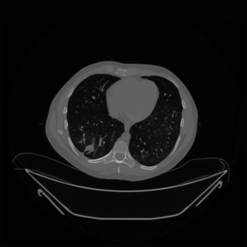
((b)) $80$ keV

((c)) $120$ keV

Figure 1: Example of a three-energy bins attenuation image. Images are displayed in Hounsfield unit.

Simulated data were generated using the forward model described in (6) and (7) with source intensity set as $\bar{h}_{i,k}=5{,}000$ (low dose) and $\bar{h}_{i,k}=10{,}000$. We implemented a fan-beam projection geometry with a $120$-degree angle, incorporating 750 detectors, each with a width of 1.2 mm, with source-to-origin and origin-to-detector distances both equal to 600 mm.

III-B Reconstruction Methods

We compared TDPS and ODPS with two two-step image domain material decomposition methods consisting of applying $\mathcal{F}^{\dagger}$ to the multi-energy image $\hat{\bm{x}}$ obtained by penalized weighted least-squares (PWLS), i.e.,

$$\hat{\bm{x}}\in\operatornamewithlimits{arg\,min}_{\bm{x}=\{\bm{x}_{k}\}}\,\frac{1}{2}\sum_{k=1}^{K}\left\|\bm{\mathcal{A}}(\bm{x}_{k})-\bm{b}_{k}\right\|_{\bm{W}_{k}}^{2}+\beta R(\bm{x})$$ (12)

$$\hat{\bm{z}}={}\mathcal{F}^{\dagger}(\hat{\bm{x}})$$

where the first term in (12) is a weighted least-squares (WLS) approximation of the negative log-likelihood $\bm{x}\mapsto-\log p_{\bm{Y}|\bm{X}=\bm{x}}(\bm{y})$, $\bm{b}_{k}=[b_{1,k},\dots,b_{I,k}]\in\mathbb{R}^{I}$ with $b_{i,k}=\log\bar{h}_{i,k}/y_{i,k}$ (with $y_{i,k}>0$), $\bm{W}\in\mathbb{R}_{+}^{I\times I}$ is a diagonal matrix of statistical weights, $R$ is a regularizer applied to the images individually or synergistically and $\beta>0$. We first considered standard WLS reconstruction ($\beta=0$) then the directional total variation (DTV) regularizer [5] which enforces structural similarities with a clean reference image (obtained by reconstructing from the non-binned data) and promotes the sparisty of the gradient. We used a separable quadratic surrogate algorithm [27] for WLS while we used a Chambolle-Pock algorithm [28] for DTV. We used $\tau=0.3$ for TDPS and $\tau=0.4$ for ODPS (cf. Section II-B2 for the definition of $\tau$). The metrics for evaluation, i.e., SSIM and PSNR, were computed with the Python library skimage.metrics.

III-C Results

Figure 2 shows material decomposition results for one slice with a $\bar{h}_{i,k}=10{,}000$ X-ray photon flux. WLS-reconstructed images appear noisy while the noise is somehow controlled on the DTV-reconstructed images, but some features appear over-smoothed, especially in the lungs. TDPS images do not appear to suffer from noise amplification or over-smoothing, as all features seem to be preserved. ODPS images are somehow similar (no noise, preserved features), but some artifacts are visible such as in the spine and some ribs showing up as soft tissues.

Bones	Soft tissues
Reference
WLS
DTV
TDPS
ODPS

Figure 2: Decomposition results on one slice with X-ray photon flux set to $\bar{h}_{i,k}=10{,}000$ for all energy bins. The first row are the reference material images used to compute the SSIM and PSNR.

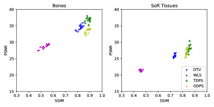
((a)) $\bar{h}_{i,k}=10,000$.

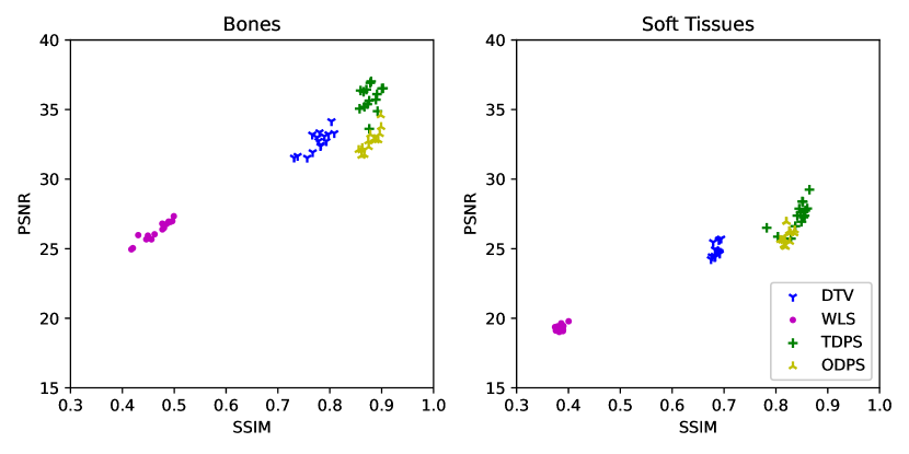
((b)) $\bar{h}_{i,k}=5,000$.

Figure 3: PSNR and SSIM of $15$ slices reconstructed from $\bar{h}_{i,k}=10,000$ and $\bar{h}_{i,k}=5,000$ photon flux.

Figure 3 presents the PSNR and SSIM metrics of $15$ material decompositions from each of the presented methods with $\bar{h}_{i,k}=5{,}000$ and $\bar{h}_{i,k}=10{,}000$. The metrics were computed for each material separately. The results seem to confirm the observations from Figure 2. Both ODPS and TDPS appear to outperform WLS and DTV, especially for $\bar{h}_{i,k}=5{,}000$, while TDPS outperforms ODPS.

IV Discussion and Conclusion

Designing a prior (or a regularization function) is a central question for solving inverse problems and generative models may offer an elegant and effective solution to this. We proposed two methods for material decomposition using a reversed DM implemented with a trained NNs as a prior, for both TDPS and ODPS. Both methods give promising results as compared with state-of-the-art techniques, especially TDPS. Early results show that TDPS outperforms ODPS. This is due to the presence of artifacts in ODPS images such as ribs interpreted as soft tissues. This phenomenon could be attributed to the smallness of our training dataset. However, it has been demonstrated in the literature that one-step methods tend to outperform two-step approaches [29, 30]. There we expect to obtain better results with ODPS in the future though fine tuning and better training (more epochs, larger database). In fact, unbeknownst to us, similar research by X. Jiang et al.  [31] was carried out at the time of preparing this paper. They used a “jumpstart” method which consists in starting the conditional diffusion on a scout decomposition and refining the computation of the gradient (11). This approach seems to remove the artifact we observed in ODPS. Further research in that direction could lead to promising results.

V Acknowledgments

This work was conducted within the France 2030 framework programmes, Centre Henri Lebesgue ANR-11-LABX-0020-01 and French National Research Agency (ANR) under grant No ANR-20-CE45-0020, and with the support of Région Bretagne.

References

- [1] R. E. Alvarez and A. Macovski, “Energy-selective reconstructions in x-ray computerised tomography,” Physics in Medicine & Biology, vol. 21, no. 5, p. 733, sep 1976.
- [2] D. S. Rigie and P. J. L. Rivière, “Joint reconstruction of multi-channel, spectral CT data via constrained total nuclear variation minimization,” Physics in Medicine & Biology, vol. 60, no. 5, p. 1741, feb 2015.
- [3] H. Gao, J.-F. Cai, Z. Shen, and H. Zhao, “Robust principal component analysis-based four-dimensional computed tomography,” Physics in Medicine & Biology, vol. 56, no. 11, p. 3181, 2011.
- [4] Y. He, L. Zeng, Q. Xu, Z. Wang, H. Yu, Z. Shen, Z. Yang, and R. Zhou, “Spectral CT reconstruction via low-rank representation and structure preserving regularization,” Physics in Medicine & Biology, vol. 68, no. 2, p. 025011, 2023.
- [5] E. Cueva, A. Meaney, S. Siltanen, and M. J. Ehrhardt, “Synergistic multi-spectral CT reconstruction with directional total variation,” Philosophical Transactions of the Royal Society A: Mathematical, Physical and Engineering Sciences, vol. 379, no. 2204, p. 20200198, 2021.
- [6] Y. Zhang, X. Mou, G. Wang, and H. Yu, “Tensor-based dictionary learning for spectral ct reconstruction,” IEEE transactions on medical imaging, vol. 36, no. 1, pp. 142–154, 2016.
- [7] A. Perelli, S. A. Garcia, A. Bousse, J.-P. Tasu, N. Efthimiadis, and D. Visvikis, “Multi-channel convolutional analysis operator learning for dual-energy CT reconstruction,” Physics in Medicine & Biology, vol. 67, no. 6, p. 065001, 2022.
- [8] Z. Wang, A. Bousse, F. Vermet, J. Froment, B. Vedel, A. Perelli, J.-P. Tasu, and D. Visvikis, “Uconnect: Synergistic spectral CT reconstruction with U-Nets connecting the energy bins,” IEEE Transactions on Radiation and Plasma Medical Sciences, 2023.
- [9] A. Bousse, V. S. S. Kandarpa, S. Rit, A. Perelli, M. Li, G. Wang, J. Zhou, and G. Wang, “Systematic review on learning-based spectral CT,” IEEE Transactions on Radiation and Plasma Medical Sciences, 2023.
- [10] J. Gondzio, M. Lassas, S.-M. Latva-Äijö, S. Siltanen, and F. Zanetti, “Material-separating regularizer for multi-energy x-ray tomography,” Inverse Problems, vol. 38, no. 2, p. 025013, 2022.
- [11] P. Dhariwal and A. Nichol, “Diffusion models beat gans on image synthesis,” Advances in neural information processing systems, vol. 34, pp. 8780–8794, 2021.
- [12] Y. Song, J. Sohl-Dickstein, D. P. Kingma, A. Kumar, S. Ermon, and B. Poole, “Score-based generative modeling through stochastic differential equations,” in International Conference on Learning Representations, 2021.
- [13] H. Chung, J. Kim, M. T. Mccann, M. L. Klasky, and J. C. Ye, “Diffusion posterior sampling for general noisy inverse problems,” in The Eleventh International Conference on Learning Representations, 2023.
- [14] C. Vazia, A. Bousse, B. Vedel, F. Vermet, Z. Wang, T. Dassow, J.-P. Tasu, D. Visvikis, and J. Froment, “Diffusion posterior sampling for synergistic reconstruction in spectral computed tomography,” in 2024 IEEE 21st international symposium on biomedical imaging (ISBI 2024). IEEE, 2024.
- [15] T. Weidinger, T. Buzug, T. Flohr, S. Kappler, and K. Stierstorfer, “Polychromatic iterative statistical material image reconstruction for photon-counting computed tomography,” International Journal of Biomedical Imaging, vol. 2016, pp. 1–15, 01 2016.
- [16] J. Ho, A. Jain, and P. Abbeel, “Denoising diffusion probabilistic models,” Advances in neural information processing systems, 2020.
- [17] Y. Song and S. Ermon, “Generative modeling by estimating gradients of the data distribution,” in Advances in Neural Information Processing Systems, H. Wallach, H. Larochelle, A. Beygelzimer, F. d'Alché-Buc, E. Fox, and R. Garnett, Eds., vol. 32. Curran Associates, Inc., 2019.
- [18] B. D. Anderson, “Reverse-time diffusion equation models,” Stochastic Processes and their Applications, vol. 12, no. 3, pp. 313–326, 1982.
- [19] A. Hyvärinen, “Estimation of non-normalized statistical models by score matching,” Journal of Machine Learning Research, vol. 6, pp. 695–709, 01 2005.
- [20] Y. Song, L. Shen, L. Xing, and S. Ermon, “Solving inverse problems in medical imaging with score-based generative models,” in International Conference on Learning Representations, 2022.
- [21] H. Chung, B. Sim, D. Ryu, and J. C. Ye, “Improving diffusion models for inverse problems using manifold constraints,” Advances in Neural Information Processing Systems (NeurIPS), 2022.
- [22] O. Ronneberger, P. Fischer, and T. Brox, “U-net: Convolutional networks for biomedical image segmentation,” in Medical Image Computing and Computer-Assisted Intervention – MICCAI 2015, N. Navab, J. Hornegger, W. M. Wells, and A. F. Frangi, Eds. Cham: Springer International Publishing, 2015, pp. 234–241.
- [23] K. He, X. Zhang, S. Ren, and J. Sun, “Deep residual learning for image recognition,” in Proceedings of the IEEE conference on computer vision and pattern recognition, 2016, pp. 770–778.
- [24] A. Vaswani, N. Shazeer, N. Parmar, J. Uszkoreit, L. Jones, A. N. Gomez, L. Kaiser, and I. Polosukhin, “Attention is all you need,” Advances in neural information processing systems, 30., 2017.
- [25] M. Ronchetti, “Torchradon: Fast differentiable routines for computed tomography,” arXiv preprint arXiv:2009.14788, 2020.
- [26] J. H. Hubbell and S. M. Seltzer, “X-ray mass attenuation coefficients, nist standard reference database 126,” [Online; accessed 01/2023]. [Online]. Available: https://www.nist.gov/pml/x-ray-mass-attenuation-coefficients/
- [27] I. Elbakri and J. Fessler, “Statistical image reconstruction for polyenergetic x-ray computed tomography,” IEEE Transactions on Medical Imaging, vol. 21, no. 2, pp. 89–99, 2002.
- [28] A. Chambolle and T. Pock, “A first-order primal-dual algorithm for convex problems with applications to imaging,” Journal of mathematical imaging and vision, vol. 40, pp. 120–145, 2011.
- [29] Y. Long and J. A. Fessler, “Multi-material decomposition using statistical image reconstruction for spectral ct,” IEEE Transactions on Medical Imaging, vol. 33, no. 8, pp. 1614–1626, 2014.
- [30] C. Mory, B. Sixou, S. Si-Mohamed, L. Boussel, and S. Rit, “Comparison of five one-step reconstruction algorithms for spectral CT,” Physics in Medicine & Biology, vol. 63, no. 23, p. 235001, nov 2018.
- [31] X. Jiang, G. J. Gang, and J. W. Stayman, “Ct material decomposition using spectral diffusion posterior sampling,” 2024.