Finite mixture copulas for modeling dependence in longitudinal count data
Abstract
Dependence modeling of multivariate count data has been receiving a considerable attention in recent times. Multivariate elliptical copulas are typically preferred in statistical literature to analyze dependence between repeated measurements of longitudinal data since they allow for different choices of the correlation structure. But these copulas lack in flexibility to model dependence and inference is only feasible under parametric restrictions. In this article, we propose the use of finite mixture of elliptical copulas in order to capture complex and hidden temporal dependency of discrete longitudinal data. With guaranteed model identifiability, our approach permits to use different correlation matrices in each component of the mixture copula. We theoretically examine the dependence properties of finite mixture of copulas, before applying them for constructing regression models for count longitudinal data. The inference of the proposed class of models is based on composite likelihood approach and the finite sample performance of the parameter estimates are investigated through extensive simulation studies. For model validation, besides the standard techniques we extended the -plot method to accommodate finite mixture of elliptical copulas. Finally, our models are applied to analyze the temporal dependency of two real world longitudinal data sets and shown to provide improvements if compared against standard elliptical copulas.
Keywords: mixture copula; temporal dependency; longitudinal data; count responses; composite likelihood.
1 Introduction
In longitudinal studies for count data, a small number of repeated count responses along with a set of multidimensional covariates are collected from a large number of independent individuals. Two main aspects of analysing such data is to find the effects of the covariates on the repeated count responses and to measure the strength of dependence between them across time. Weiss (2005) or Sutradhar (2011) are some of the excellent books which provide with concepts and ideas for developing correlation models for discrete longitudinal data. Gibbons et al. (2010) reviewed recent developments of discrete longitudinal data analysis. In the context of count data, some of the seminal works includes Thall & Vail (1990) and Jowaheer & Sutradhar (2002), who considered mixed effect approaches for modeling longitudinal count data. Sutradhar (2003) provided different estimation techniques for count regression models based on generalized estimating equations. Xu et al. (2007) proposed a state space model to analyze count longitudinal data with serial correlation. But these mixed model approaches comes with computational complexities due to the involvement of multidimensional random effects.
Due to the non-Gaussian form of count longitudinal data, the interest in the copula framework is increasingly growing among statisticians because they offer great flexibility to model multivariate distributions and interprets the dependence between several random variables in a natural way. Under this modeling approach a wide range of dependence structures can be introduced into a regression model while the marginals can be selected arbitrarily. In the literature, Nikoloulopoulos & Karlis (2009) and Nikoloulopoulos & Karlis (2010) were the first to show some of the successful applications of copulas to multivariate count data. As described by the authors, some of the desirable properties of copulas are no longer valid when they are directly applied to discrete data such as dependence measures depend on the marginal distributions. But modeling poses no issue since according to Sklar’s theorem the copula can be uniquely identified over the product range of the marginals. Sun et al. (2008) recommended the use of elliptical copulas to model non-Gaussian longitudinal data since they account for within-subject dependencies through the correlation matrices which can handle its time series behavior. Shi (2012) and Shi & Valdez (2014) extended their approach to model longitudinal insurance claim data. But these copulas are not flexible enough to capture complex dependence patterns due to their parametric restrictions. Several authors proposed the use of vine copulas to overcome the limitations of standard multivariate copulas but they often involves too many parameters to estimate which can be computationally challenging in several scenarios. Since our approach is not based on vine copulas we do not provoke any unnecessary citations. Recently there has been research that combine copulas with a finite mixture model to understand complex dependence patterns as well as to increase the model flexibility. Finite mixture model in general represents a probabilistic model which is explained as a weighted sum of a few parametric densities. They are very useful for uncovering hidden structures in the data (e.g. see Peel & McLachlan (2000) or Karlis (2019)). Yang et al. (2022) used a time-varying mixture copula model in a semiparametric set up to analyze the time series behaviour of stock market data.
In this article we focus our attention to model the unknown correlation structure of longitudinal count data. Our motivation comes from the fact that in a mixture of elliptical copulas, different correlation structures can be used in each component copulas and it theoretically ensures identifiability of the model. The magnitudes of the weights in a mixture copula model signify the importance of the corresponding component copulas. Moreover, the model parameters can be efficiently estimated using the composite likelihood method followed by a two stage procedure. The contribution to this manuscript is two fold. Firstly, we explicitly derive the dependence properties of mixture copula models under both continuous and discrete setup. As far as we reviewed the literature, mixture copulas have been applied to discrete data but their dependence properties under the discrete setup were not explicitly derived. Recently Safari-Katesari et al. (2020) introduced population version of Spearman’s rho for discrete data and applied some well known Archimedean copulas to model bivariate count data. Secondly, in our applications we consider regression models for longitudinal count data with the temporal dependencies described by the mixture of elliptical copulas.
Rest of the article is organized as follows. In Section 2, we review some standard definitions of mixture and elliptical copulas. In Section 3, we derive the theoretical properties such as Kendall’s tau and Spearman’s rho for a general mixture copula under both continuous and discrete case. Section 4 describes some standard marginal regression models generally used for modeling longitudinal count data. Two stage composite likelihood estimation method for mixture copula based count regression models are discussed in Section 5. In Section 6, we discuss some standard model validation techniques and also extend the -plot method of model validation for finite mixture of elliptical copulas. Some rigorous simulation studies are conducted in Section 7 to gauge the finite sample performances of our proposed class of models under different sample sizes. In Section 8 we apply our methods to model the temporal dependency of two real world data sets. We also compared the fits of mixture copulas with standard elliptical copulas and showed substantial improvements. Based on the derived expressions of Kendall’s tau and Spearman’s rho, we estimated the concordance matrices of these two data sets and showed that they are very close to their empirical versions. Finally we conclude this article with a general discussion in Section 9.
2 The K-finite mixture of multivariate copulas
Mixture models have been widely studied in the statistical literature; see for example the books by Titterington et al. (1985); Böhning (1999) and Frühwirth-Schnatter (2006), among others. McLachlan et al. (2019) provided with the basics of mixture modeling and its applications. As more flexible multivariate distributions can be obtained by mixing different distributions of the same dimension (might not be from the same family), similarly one can use mixture of different copulas to introduce different dependence characteristics in a statistical model. In many real-life applications, a single parametric copula might be insufficient to capture all important features when performing analysis. Finite mixture copula models have been previously studied in the literature (we refer to the readers to see Arakelian & Karlis (2014); Kosmidis & Karlis (2016) or Zhuang et al. (2022)).
A K-finite mixture copula is defined as
| (2.1) |
where denotes a single -dimensional multivariate copula component which has a mixture weight , and is a pre-defined hyperparameter. It is straight forward to check that the distribution function in (2.1) is a copula. The density function of the mixture copula can be simply obtained as
| (2.2) |
where denotes all dependence parameters, and contains the copula parameters of the -th component. The choice of the copula components in the mixture (2.1) is arbitrary, but in this article we restrict to the multivariate elliptical copulas.
2.1 Elliptical copulas
Multivariate copulas generated from elliptical distributions as multivariate normal or Student- are popular in the literature of statistics and econometrics for their simplicity in terms of parametric inference (see, Xue-Kun Song (2000); Demarta & McNeil (2005)). Frahm et al. (2003) discussed the dependence structures generated by elliptical distributions and their limitations. We proceed with some standard definitions as follows.
Definition 2.1
A -dimensional copula is said to be a gaussian copula if
| (2.3) |
where denotes the inverse of the CDF of distribution.
Definition 2.2
A -dimensional copula is said to be a Student- copula if
| (2.4) |
where denotes the inverse of the CDF of distribution.
Student- copula has an additional degrees of freedom parameter , which accounts for possible tail dependence in the data. We consider the mixture of Gaussian and Student- copulas for modeling the temporal dependency of longitudinal count data. As Sun et al. (2008) emphasized, elliptical copulas are more useful when the dimension of the data is moderate to high since all lower dimensional sub-copulas stay in the same parametric family (Frees & Wang (2006)).
2.2 Model identifiability
Identifiability of finite mixture models is considered to be a critical aspect in statistical analysis. It is a key property that determines if a statistical model’s true parameters can be learned asymptotically with the number of samples. A parametric family of densities is identifiable if distinct values of the parameter determine distinct members of the family of densities , where is the specified parameter space. Identifiability of parametric mixture densities have been studied in the seminal works by Teicher (1963) and Yakowitz & Spragins (1968). They pointed out that most finite mixtures of continuous densities are identifiable; an exception is a mixture of uniform densities. In practice therefore one need specific parametric restrictions on so that the likelihood of the mixture does not change under a permutation of component labels. In this paper we implement copulas to discrete margins which poses identifiability issues as one could use different copulas to construct the same discrete probability distribution. Genest & Nešlehová (2007) highlighted the consequences in inference for the lack of uniqueness of the copula under discrete margins. Uniqueness of copulas is only guaranteed at the range of marginal distibutions according to Sklar’s theorem, which is the entire range of for continuous data and some countable values on for discrete data, so the copula can only be identified on the support and is not unique outside the support of the marginal CDF. Hence, it is reasonable to proceed by using one particular choice of copulas in applications. Holzmann et al. (2006) discussed some theoretical results on identifiability of mixture models constructed from elliptical distributions. They showed that elliptical mixtures are identifiable. Liu et al. (2023) argued that finite mixture of gaussian copulas is identifiable followed from the fact that the quantiles have the distribution of a multivariate normal mixture. Therefore, in this paper we only consider the mixture of elliptical copulas within their own parametric family. Another reason for that is they are easy to simulate and have simpler parametric inference using composite likelihood which will be discussed latter on.
3 Dependence properties
Here we provide a comprehensive theoretical analysis of mixture copula models for both continuous and discrete margins. The results presented in this section are for a general mixture copula model. If the dependence between two variables is such that if one variable increases then the other tends to increase or decrease, then it is referred as monotone association. Kendall’s tau and Spearman’s rho are the most widely used measures of monotone association, which are based on concordance and discordance. Although multivariate extensions of these measures have been discussed by several authors like Nelsen (2002) or Joe (1990), but here we focus on the bivariate case. For continuous random variables, dependence as measured by Kendall’s tau or Spearman’s rho is associated only with the copula parameters (see, Nelsen (2006)). Therefore the dependence parameters , of the mixture copulas in (2.2) can be interpreted with respect to Kendall’s tau and Spearman’s rho, which are bounded in the interval . First we derive the population versions of Kendall’s tau and Spearman’s rho for continuous random variables as follows.
Theorem 3.1
Let be a bivariate continuous random vector having dependence of finite mixture copula defined in (2.1), with marginal distribution functions . The population version of Kendall’s tau for and is given by
| (3.1) |
where is the concordance function defined for copulas and and is the Kendall’s tau corresponding to copula , for .
Note that the concordance function is symmetric in its arguments for a continuous random vector (Nelsen (2006); Arakelian & Karlis (2014)), but this doesn’t hold for the discrete case.
Corollary 3.1
For mixture of Gaussian and Student- copula, the population version of Kendall’s tau can be obtained in a closed form expression as -
| (3.2) |
where is the correlation parameter of bivariate Gaussian or Student- copula, for .
Theorem 3.2
Let be a bivariate continuous random vector having dependence of finite mixture copula defined in (2.1), with marginal distribution functions . The population version of Spearman’s rho for and is given by
| (3.3) |
where is the Spearman’s rho corresponding to copula , for .
Expression of Spearman’s rho for Gaussian mixture copula can be obtained in a closed form, but for Student- no closed form is available (see, Joe (2014)).
When the marginal distributions are discrete, these concordance based measures depends on the marginal distributions as well as the copula. Denuit & Lambert (2005) and Mesfioui & Tajar (2005) studied the population version of Kendall’s tau applied to discrete data, which is not distribution free and has a range narrower than . Nikoloulopoulos & Karlis (2010) previously derived the population version of Kendall’s tau under discrete marginals. Recently, Safari-Katesari et al. (2020) derived the population version of Spearman’s rho followed by continuous extension of discrete random variables. Followed from these, we derive the population versions of these concordance measures of mixture of copulas for the discrete case. Note that when the marginal distributions are discrete, the probability of tie is positive which needs to be considered in the derivation.
Theorem 3.3
Let be a bivariate integer valued random vector having dependence of finite mixture copula defined in (2.1), with marginal distribution functions and mass functions . The population version of Kendall’s tau for and is given by
| (3.4) |
| (3.5) | ||||
| (3.6) |
| (3.7) |
Theorem 3.4
Let be a bivariate integer valued random vector having dependence of finite mixture copula defined in (2.1), with marginal distribution functions and mass functions . The population version of Spearman’s rho for and is given by
| (3.8) |
| (3.9) |
and is the joint probability mass function same as defined in (3.3).
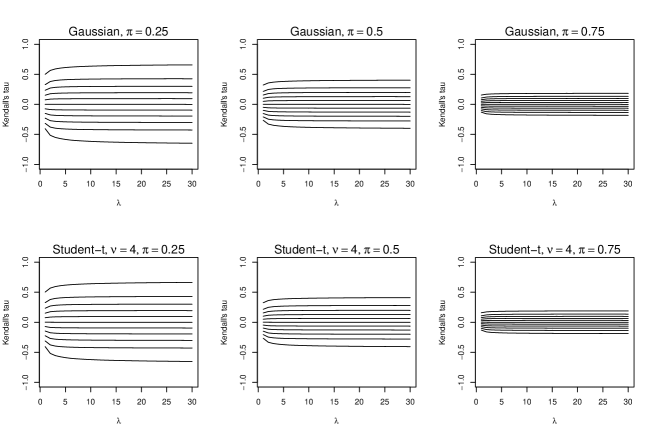
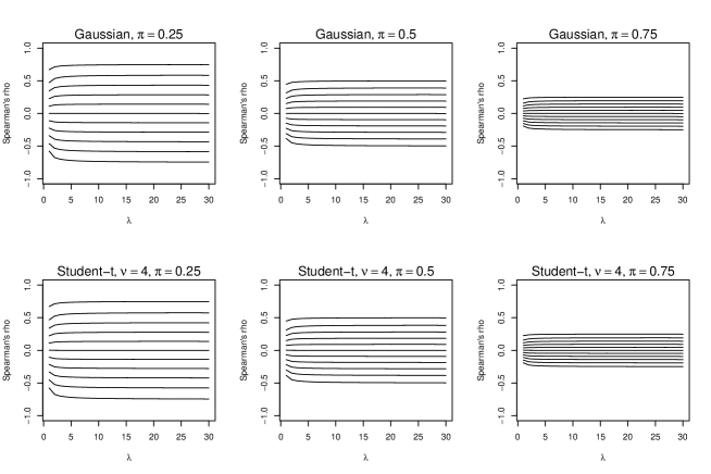
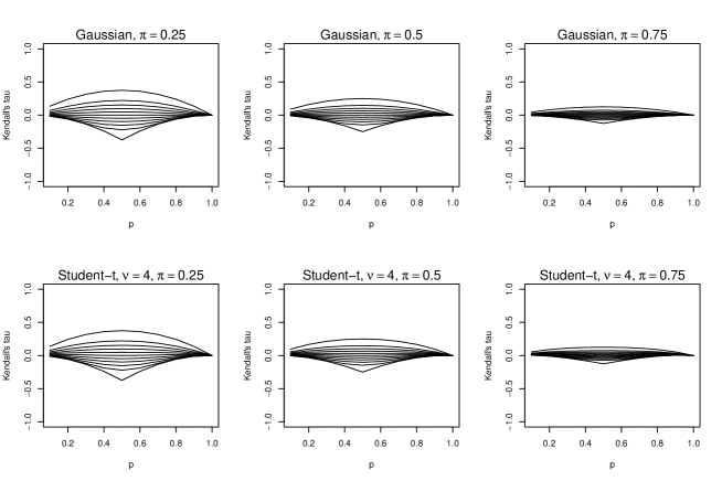
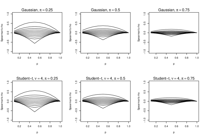
It is evident that the Spearman’s rho of convex combination of copulas equals the convex combination of the individual Spearman’s rho for both continuous and discrete case. The derived results help us to clarify that in the discrete case the marginals do affect the dependence measures. Based on the expressions in (3.1), (3.3), (3.4) and (3.8) one can see that even if the component copulas imply independence, the resulting mixture may imply dependence. In Figures 1, 2, 3 and 4 we provide the plotted values of Kendall’s tau and Spearman’s rho for different elliptical mixture copulas and different marginal distributions. We consider component mixture and in the first component copula we set the correlation parameter (i.e. independence copula). The correlation parameter of the second copula component is varied over . When the marginal distributions are Poisson with the same parameter for each marginal, we can see that for their values greater than , association with the values of Kendall’s tau and Spearman’s rho is negligible. When the marginal distributions are Bernoulli with the same parameter for each marginal, association with the values of Kendall’s tau and Spearman’s rho is minimum when the proportion of success is . Note that elliptical mixture copulas are symmetric by construction and permits both negative and positive dependence. As the mixing proportion with the independence copula increases, the values of Kendall’s tau and Spearman’s rho shrink towards zero.
Lastly we need to discuss the tail dependence of a mixture copula. Tail dependence quantifies the degree of dependence in the joint lower or joint lower of a multivariate distribution. Here we consider the bivariate tail dependence only, but there are multivariate extensions to the concept in the literature (see, Jaworski et al. (2010)). For a bivariate distribution, tail dependence is defined as the limiting probability of exceeding a certain threshold by one margin given that the other margin has already exceeded that threshold. Upper and lower tail dependence coefficients are of interest for a bivariate distribution or copula.
Definition 3.1
Let be a bivariate random vector with with marginal distribution functions and copula . Then the upper tail and lower tail dependence coefficients are defined by
| (3.10) |
| (3.11) |
where provided the above limits exist.
The copula is said to have upper or lower tail dependence if . If or , we say has no upper or lower tail dependence, respectively. The following Theorem states the tail behavior of bivariate mixture copulas.
Theorem 3.5
Let and be the tail dependence coefficients of the component copula , provided these exists and be the mixing proportion for . Then the upper and lower tail dependence coefficients are given as
| (3.12) |
4 Modeling longitudinal count data
Suppose that be a non-negative integer valued dependent random vector for the -th subject, where denotes the observation at time . Let be a -dimensional vector of covariates observed for the -th subject at time and is the vector of regression parameters. In the longitudinal set-up, the components of the vector are repeated responses, which are likely to be correlated. Since the true correlation structure of these repeated measurements always remains unknown, copula framework is very useful to analyse and investigate the temporal association. Since for discrete random variables the copula is uniquely identified in in the product range of the marginals, we assume restrictively that the marginal models for the repeated responses are correctly specified. The two most commonly applied distributions for count responses are Poisson and Negative Binomial distributions. Poisson regression assumes that the repeated count responses marginally follows a Poisson distribution with CDF
| (4.1) |
where . Since poisson distribution doesn’t allow for over dispersion in longitudinal count data, we also consider Negative Binomial regression model for the count responses. The CDF of a Negative Binomial marginal can be written as
| (4.2) |
where and . Point to be noted that both of these distributions are defined on same support of non-negative integers.
Once the marginals are chosen using standard diagnostics methods such as likelihood ratio test, an appropriate multivariate copula can be selected to analyze the dependence between repeated measurements. Since in our approach we employ mixture of elliptical copulas it allows to use different correlation structures into each copula component. This can be nicely interpreted as we can show which correlation structure is present in the data set in what proportion. Common choices for modeling serial dependence in longitudinal data are auto-regressive (), moving average () or exchangeable () correlation structures. Under the structure, the correlation between the errors on a subject decline exponentially with the distance between the observations. In terms of the correlation matrix in the elliptical copulas, it can be expressed as
| (4.3) |
where is the auto-regressive parameter. Under the exchangeable structure, the correlation between the errors remains constant and time invariant. Thus, considering elliptical copulas our methods can be extended to the unbalanced longitudinal data where the number of measurements per subject can be different. In the next section we describe the two stage estimation method for our mixture copula based models designed for longitudinal count data.
5 Parameter estimation
Since the count repeated measurements are discrete, the joint probability mass function of involves a -times folded sum, which is difficult to evaluate in practice (see, Song et al. (2009), Madsen & Fang (2011)). Since for multivariate elliptical copulas all parameters can be identified from its lower dimensional sub-copulas, same holds true for their finite mixtures. This can be shown algebraically from the construction of mixture distributions. To circumvent the computational issues composite likelihood methods (CML) can be employed for the considered class of models. With this method, pseudolikelihoods are constructed and then maximized using the consecutive pairs of observations, and hence also called as pairwise likelihood estimation (le Cessie & Van Houwelingen (1994)). Recent overviews on composite likelihood estimation can be found in Varin & Czado (2010) and Varin et al. (2011). In contrast to a full likelihood approach, the composite likelihood formulations only requires the specification of bivariate pairs of observations.
In order to simplify the computational efforts to estimate the model parameters, we employ the two stage estimation procedure of the composite likelihood as described in Zhao & Joe (2005) and Diao & Cook (2014). Due to the copula structure of the dependence models, this method produces consistent estimates of the model parameters and their corresponding robust standard errors. Let be the marginal probability mass function of the response variable and be the vector of parameters corresponding to the marginals. Then in the first stage, under working independence assumption we estimate the marginal parameters by maximizing
| (5.1) |
and then using the parameter estimates from (5.1), we compute the uniform samples: , where , . In the second stage, the estimates are inserted into composite likelihood of the form:
| (5.2) |
and then maximized with respect to the set of parameters , to obtain the estimates of the association parameters. Shi et al. (2016) previously used similar estimation estimation strategy to model multilevel insurance claim data using Gaussian copula. It has been a standard practice to estimate model parameters of mixture distributions through EM type algorithms. But here we proceed by numerical maximization of the objective functions in (5.1) and (5) with box constraints (see, MacDonald (2014)). This method is alternatively known as inference function of margins. The standard error of the parameter estimates can be numerically obtained from the estimated sandwich information matrix (Godambe information matrix) of the form:
| (5.3) |
where is a block diagonal matrix and is a symmetric positive definite matrix. The explicit forms of these matrices can be found in Zhao & Joe (2005) or Joe (2014). To estimate the parameter we use optim function, and to estimate the information matrix associted with the parameter estimates we use numderiv function in R.
6 Model Validation
The validation of copula based regression models has been widely discussed in the literature (see, Genest et al. (2009) or Ko & Hjort (2019)). To determine which model is best suited for a data set, standard model selection techniques such as AIC (Akaike information criterion) and BIC (Bayesian information criterion) are often used. Varin & Vidoni (2005) and Gao & Song (2010) modified these two in the case of composite likelihood estimation. These are defined as:
| (6.1) |
In our applications, we prefer models with smaller values of these criteria. Since we consider mixture of elliptical copulas to model temporal dependencies of count longitudinal data, additionally we can validate the model assumptions utilizing the -plot method by Sun et al. (2008) and Shi (2012).
We propose a simple modification of the -plot method for mixture of elliptical copulas utilizing the definition of the mixture distribution. This method method was designed to test the elliptical symmetry of multivariate distributions (see, Li et al. (1997)) using invariant statistics under orthogonal transformations. Shi & Valdez (2014) used this method to validated elliptical assumption of the underlying copula for unbalanced longitudinal count data. The null hypothesis of a -plot is that a sample is from an elliptical multivariate distribution. Such hypothesis could be tested for mixture of elliptical distributions as well. The procedure is given as follows -
-
•
For each unit , transform the count variables on uniform scale by for . Where is the estimated marginal parameter from the first stage. Now the transformed data can be considered as a realization of the mixture of elliptical copulas.
-
•
Compute the quantiles of by , where denotes the CDF of the -th marginal associated with the elliptical copula. If the copula is well specified, then the vector would follow a mixture of elliptical distributions.
-
•
Let be an indicator representing whether the -th unit comes from the -th component of the finite mixture of elliptical distributions as
(6.2) and be the expected value of . This can also be interpreted as the posterior probability of -th unit belonging to the -th component of the mixture. Hence we estimate by
(6.3) Where is the estimated value of . Now the -th units is most likely to be coming from the -th component of the mixture if .
-
•
After identifying the -th component distribution for the -th unit, we calculate the vector and construct the -statistic as
(6.4) where . Thus should be from a standard -distribution with degrees of freedom.
-
•
Repeat the above procedure for all units in the sample and define the transformed variable for . If the copula captures the dependence structure properly, then should be a random sample from distribution. Therefore, we plot the sample quantiles of against the theoretical quantiles to graphically visualize the goodness-of-fit of the model.
7 Simulation studies
In this section we undertake some simulations to monitor the finite sample performance of the proposed mixture copula models designed for count longitudinal data. In our simulations as well as applications, we set the number of components of the mixture to . We consider two marginal distributions as discussed in Section 4. The specifications of the marginal models are given as
| (7.1) |
where the dimension of each units is fixed to . We assign same values of the regression coefficients for both of this marginals as, and set the over dispersion parameter for Negative Binomial marginals to . The fixed covariates are generated as , (discrete uniform distribution) and the time points for , , respectively. We consider two different sample sizes in our simulations as . For the mixture copula models we consider one component copula to be autoregressive and another to be exchangeable (parameterized as ). We set the parameters for each multivariate copulas as (under structure) and (under structure). We also consider choices for the mixing proportions as . This parameter essentially interprets which correlation structure is present in the data set in what proportion. This -set parameter allows for a wide range of dependence in class of models. Generating the data sets using standard probability transformations method, we estimate the model parameters using the two stage method discussed in Section 5. We repeat the whole process for times and report the findings.
| m = 200 | m = 500 | ||||||||||
|---|---|---|---|---|---|---|---|---|---|---|---|
| Parameters | True Value | Mean | Bias | SD | SE | RMSE | Mean | Bias | SD | SE | RMSE |
| 0.25 | 0.2555 | 0.0055 | 0.1132 | 0.1333 | 0.1133 | 0.2549 | 0.0049 | 0.0759 | 0.0843 | 0.0761 | |
| 1.0 | 0.9964 | -0.0036 | 0.0893 | 0.0856 | 0.0894 | 1.0006 | 0.0006 | 0.0559 | 0.0543 | 0.0559 | |
| 0.5 | 0.5011 | 0.0011 | 0.0525 | 0.0506 | 0.0525 | 0.5008 | 0.0008 | 0.0321 | 0.0323 | 0.0322 | |
| 0.5 | 0.5006 | 0.0006 | 0.0257 | 0.0242 | 0.0257 | 0.4993 | -0.0007 | 0.0160 | 0.0154 | 0.0160 | |
| -0.5 | -0.5004 | -0.0004 | 0.0122 | 0.0132 | 0.0122 | -0.5005 | -0.0005 | 0.0081 | 0.0084 | 0.0081 | |
| 0.3 | 0.3570 | 0.0570 | 0.1687 | 0.1478 | 0.1781 | 0.3302 | 0.0302 | 0.1156 | 0.0958 | 0.1195 | |
| 0.7 | 0.6935 | -0.0065 | 0.1018 | 0.1075 | 0.1020 | 0.6934 | -0.0066 | 0.0755 | 0.0737 | 0.0757 | |
| 0.50 | 0.4884 | -0.0116 | 0.1182 | 0.1289 | 0.1188 | 0.4929 | -0.0071 | 0.0816 | 0.0819 | 0.0819 | |
| 1.0 | 0.9966 | -0.0034 | 0.0879 | 0.0878 | 0.0880 | 1.0016 | 0.0016 | 0.0544 | 0.0554 | 0.0545 | |
| 0.5 | 0.5027 | 0.0027 | 0.0526 | 0.0517 | 0.0527 | 0.5017 | 0.0017 | 0.0342 | 0.0328 | 0.0343 | |
| 0.5 | 0.5003 | 0.0003 | 0.0254 | 0.0249 | 0.0254 | 0.4989 | -0.0011 | 0.0155 | 0.0157 | 0.0156 | |
| -0.5 | -0.5003 | -0.0003 | 0.0135 | 0.0136 | 0.0135 | -0.4996 | 0.0004 | 0.0087 | 0.0086 | 0.0087 | |
| 0.3 | 0.3179 | 0.0179 | 0.0969 | 0.0721 | 0.0985 | 0.3109 | 0.0109 | 0.0593 | 0.0478 | 0.0603 | |
| 0.7 | 0.6862 | -0.0138 | 0.1411 | 0.1404 | 0.1417 | 0.6963 | -0.0037 | 0.1035 | 0.0994 | 0.1036 | |
| 0.75 | 0.7247 | -0.0253 | 0.1119 | 0.1243 | 0.1147 | 0.7502 | 0.0002 | 0.0687 | 0.0772 | 0.0687 | |
| 1.0 | 1.0023 | 0.0023 | 0.0900 | 0.0888 | 0.0901 | 1.0004 | 0.0004 | 0.0586 | 0.0566 | 0.0586 | |
| 0.5 | 0.4985 | -0.0015 | 0.0531 | 0.0527 | 0.0531 | 0.4997 | -0.0003 | 0.0351 | 0.0335 | 0.0352 | |
| 0.5 | 0.4988 | -0.0012 | 0.0253 | 0.0252 | 0.0253 | 0.4998 | -0.0002 | 0.0162 | 0.0160 | 0.0162 | |
| -0.5 | -0.4993 | 0.0007 | 0.0151 | 0.0139 | 0.0151 | -0.5001 | -0.0001 | 0.0090 | 0.0089 | 0.0090 | |
| 0.3 | 0.3085 | 0.0085 | 0.0532 | 0.0502 | 0.0539 | 0.3077 | 0.0077 | 0.0348 | 0.0302 | 0.0356 | |
| 0.7 | 0.6607 | -0.0393 | 0.1775 | 0.2173 | 0.1818 | 0.6844 | -0.0156 | 0.1434 | 0.1654 | 0.1443 | |
| m = 200 | m = 500 | ||||||||||
|---|---|---|---|---|---|---|---|---|---|---|---|
| Parameters | True Value | Mean | Bias | SD | SE | RMSE | Mean | Bias | SD | SE | RMSE |
| 0.25 | 0.2695 | 0.0195 | 0.1233 | 0.1545 | 0.1249 | 0.2495 | -0.0005 | 0.0865 | 0.0960 | 0.0865 | |
| 1.0 | 0.9958 | -0.0042 | 0.0859 | 0.0857 | 0.0860 | 0.9995 | -0.0005 | 0.0536 | 0.0541 | 0.0536 | |
| 0.5 | 0.4981 | -0.0019 | 0.0518 | 0.0504 | 0.0518 | 0.5040 | 0.0040 | 0.0319 | 0.0320 | 0.0321 | |
| 0.5 | 0.5018 | 0.0018 | 0.0236 | 0.0242 | 0.0237 | 0.4990 | -0.0010 | 0.0150 | 0.0153 | 0.0150 | |
| -0.5 | -0.5004 | -0.0004 | 0.0127 | 0.0132 | 0.0127 | -0.4997 | 0.0003 | 0.0081 | 0.0084 | 0.0081 | |
| 0.3 | 0.3525 | 0.0525 | 0.1959 | 0.2016 | 0.2028 | 0.3232 | 0.0232 | 0.1353 | 0.1457 | 0.1373 | |
| 0.7 | 0.7006 | 0.0006 | 0.1291 | 0.1580 | 0.1291 | 0.7047 | 0.0047 | 0.1044 | 0.1166 | 0.1045 | |
| 0.50 | 0.5003 | 0.0003 | 0.1329 | 0.1479 | 0.1329 | 0.4937 | -0.0063 | 0.0886 | 0.0920 | 0.0888 | |
| 1.0 | 0.9998 | -0.0002 | 0.0858 | 0.0812 | 0.0858 | 1.0019 | 0.0019 | 0.0578 | 0.0554 | 0.0578 | |
| 0.5 | 0.5020 | 0.0020 | 0.0516 | 0.0516 | 0.0517 | 0.4968 | -0.0032 | 0.0338 | 0.0328 | 0.0340 | |
| 0.5 | 0.4992 | -0.0008 | 0.0240 | 0.0245 | 0.0240 | 0.4998 | -0.0002 | 0.0159 | 0.0157 | 0.0159 | |
| -0.5 | -0.4994 | 0.0006 | 0.0137 | 0.0136 | 0.0137 | -0.4996 | 0.0004 | 0.0082 | 0.0086 | 0.0082 | |
| 0.3 | 0.3237 | 0.0237 | 0.1249 | 0.1144 | 0.1271 | 0.3055 | 0.0055 | 0.0682 | 0.0699 | 0.0684 | |
| 0.7 | 0.6899 | -0.0101 | 0.1666 | 0.2288 | 0.1669 | 0.7042 | 0.0042 | 0.1245 | 0.1580 | 0.1246 | |
| 0.75 | 0.7222 | -0.0278 | 0.1223 | 0.1546 | 0.1255 | 0.7320 | -0.0180 | 0.0841 | 0.0928 | 0.0860 | |
| 1.0 | 0.9967 | -0.0033 | 0.0942 | 0.0889 | 0.0943 | 1.0041 | 0.0041 | 0.0575 | 0.0563 | 0.0576 | |
| 0.5 | 0.5033 | 0.0033 | 0.0521 | 0.0524 | 0.0522 | 0.4989 | -0.0011 | 0.0318 | 0.0333 | 0.0318 | |
| 0.5 | 0.5006 | 0.0006 | 0.0260 | 0.0250 | 0.0260 | 0.4988 | -0.0012 | 0.0162 | 0.0159 | 0.0162 | |
| -0.5 | -0.5010 | -0.0010 | 0.0149 | 0.0140 | 0.0149 | -0.4996 | 0.0004 | 0.0089 | 0.0089 | 0.0089 | |
| 0.3 | 0.3119 | 0.0119 | 0.0627 | 0.0891 | 0.0638 | 0.3057 | 0.0057 | 0.0434 | 0.0512 | 0.0438 | |
| 0.7 | 0.6617 | -0.0383 | 0.1894 | 0.2880 | 0.1932 | 0.6714 | -0.0286 | 0.1535 | 0.2145 | 0.1561 | |
| m = 200 | m = 500 | ||||||||||
|---|---|---|---|---|---|---|---|---|---|---|---|
| Parameters | True Value | Mean | Bias | SD | SE | RMSE | Mean | Bias | SD | SE | RMSE |
| 0.25 | 0.2611 | 0.0111 | 0.1188 | 0.1314 | 0.1193 | 0.2466 | -0.0034 | 0.0775 | 0.0832 | 0.0775 | |
| 1.0 | 1.0117 | 0.0117 | 0.1153 | 0.1212 | 0.1159 | 0.9975 | -0.0025 | 0.0771 | 0.0774 | 0.0771 | |
| 0.5 | 0.4933 | -0.0067 | 0.0800 | 0.0808 | 0.0802 | 0.5034 | 0.0034 | 0.0517 | 0.0514 | 0.0518 | |
| 0.5 | 0.4985 | -0.0015 | 0.0366 | 0.0370 | 0.0366 | 0.4992 | -0.0008 | 0.0230 | 0.0236 | 0.0230 | |
| -0.5 | -0.5017 | -0.0017 | 0.0189 | 0.0186 | 0.0190 | -0.4997 | 0.0003 | 0.0125 | 0.0117 | 0.0125 | |
| 4.0 | 4.1369 | 0.1369 | 0.5739 | 0.5530 | 0.5900 | 4.0512 | 0.0512 | 0.3504 | 0.3434 | 0.3541 | |
| 0.3 | 0.3555 | 0.0555 | 0.1738 | 0.1348 | 0.1825 | 0.3247 | 0.0247 | 0.1217 | 0.0953 | 0.1242 | |
| 0.7 | 0.6994 | -0.0006 | 0.1124 | 0.1088 | 0.1124 | 0.7006 | 0.0006 | 0.0785 | 0.0721 | 0.0785 | |
| 0.50 | 0.4910 | -0.0090 | 0.1191 | 0.1297 | 0.1195 | 0.4926 | -0.0074 | 0.0753 | 0.0813 | 0.0757 | |
| 1.0 | 1.0040 | 0.0040 | 0.1243 | 0.1236 | 0.1243 | 0.9998 | -0.0002 | 0.0788 | 0.0789 | 0.0788 | |
| 0.5 | 0.4912 | -0.0088 | 0.0824 | 0.0822 | 0.0829 | 0.5015 | 0.0015 | 0.0529 | 0.0524 | 0.0529 | |
| 0.5 | 0.5001 | 0.0001 | 0.0370 | 0.0376 | 0.0370 | 0.4995 | -0.0005 | 0.0237 | 0.0240 | 0.0237 | |
| -0.5 | -0.5014 | -0.0014 | 0.0194 | 0.0192 | 0.0195 | -0.4995 | 0.0005 | 0.0127 | 0.0122 | 0.0127 | |
| 4.0 | 4.2174 | 0.2174 | 0.6299 | 0.5866 | 0.6663 | 4.0615 | 0.0615 | 0.3463 | 0.3565 | 0.3518 | |
| 0.3 | 0.3315 | 0.0315 | 0.1139 | 0.0783 | 0.1181 | 0.3087 | 0.0087 | 0.0617 | 0.0488 | 0.0623 | |
| 0.7 | 0.6858 | -0.0142 | 0.1448 | 0.1460 | 0.1455 | 0.7008 | 0.0008 | 0.1054 | 0.1008 | 0.1054 | |
| 0.75 | 0.7221 | -0.0279 | 0.1174 | 0.1228 | 0.1207 | 0.7422 | -0.0078 | 0.0745 | 0.0777 | 0.0749 | |
| 1.0 | 1.0007 | 0.0007 | 0.1322 | 0.1267 | 0.1322 | 0.9969 | -0.0031 | 0.0827 | 0.0803 | 0.0828 | |
| 0.5 | 0.4999 | -0.0001 | 0.0832 | 0.0840 | 0.0832 | 0.5005 | 0.0005 | 0.0507 | 0.0533 | 0.0507 | |
| 0.5 | 0.4980 | -0.0020 | 0.0409 | 0.0383 | 0.0409 | 0.5002 | 0.0002 | 0.0260 | 0.0245 | 0.0260 | |
| -0.5 | -0.5010 | -0.0010 | 0.0191 | 0.0198 | 0.0191 | -0.4995 | 0.0005 | 0.0124 | 0.0125 | 0.0124 | |
| 4.0 | 4.1623 | 0.1623 | 0.6292 | 0.5924 | 0.6498 | 4.0639 | 0.0639 | 0.3554 | 0.3677 | 0.3611 | |
| 0.3 | 0.3207 | 0.0207 | 0.0616 | 0.0528 | 0.0650 | 0.3080 | 0.0080 | 0.0401 | 0.0308 | 0.0409 | |
| 0.7 | 0.6518 | -0.0482 | 0.1770 | 0.2146 | 0.1834 | 0.6816 | -0.0184 | 0.1456 | 0.1524 | 0.1467 | |
| m = 200 | m = 500 | ||||||||||
|---|---|---|---|---|---|---|---|---|---|---|---|
| Parameters | True Value | Mean | Bias | SD | SE | RMSE | Mean | Bias | SD | SE | RMSE |
| 0.25 | 0.2651 | 0.0151 | 0.1189 | 0.1413 | 0.1199 | 0.2500 | 0.0000 | 0.0823 | 0.0947 | 0.0823 | |
| 1.0 | 0.9921 | -0.0079 | 0.1229 | 0.1221 | 0.1231 | 0.9956 | -0.0044 | 0.0812 | 0.0776 | 0.0814 | |
| 0.5 | 0.4983 | -0.0017 | 0.0851 | 0.0811 | 0.0851 | 0.5018 | 0.0018 | 0.0540 | 0.0515 | 0.0541 | |
| 0.5 | 0.5012 | 0.0012 | 0.0385 | 0.0372 | 0.0385 | 0.5006 | 0.0006 | 0.0244 | 0.0237 | 0.0244 | |
| -0.5 | -0.4991 | 0.0009 | 0.0179 | 0.0184 | 0.0180 | -0.5000 | 0.0000 | 0.0121 | 0.0117 | 0.0121 | |
| 4.0 | 4.1597 | 0.1597 | 0.6878 | 0.6176 | 0.7061 | 4.0586 | 0.0586 | 0.3596 | 0.3803 | 0.3643 | |
| 0.3 | 0.3580 | 0.0580 | 0.1988 | 0.2019 | 0.2071 | 0.3168 | 0.0168 | 0.1362 | 0.1314 | 0.1372 | |
| 0.7 | 0.7010 | 0.0010 | 0.1237 | 0.1486 | 0.1237 | 0.7053 | 0.0053 | 0.0947 | 0.1018 | 0.0949 | |
| 0.50 | 0.5005 | 0.0005 | 0.1375 | 0.1444 | 0.1375 | 0.4974 | -0.0026 | 0.0906 | 0.0909 | 0.0906 | |
| 1.0 | 0.9911 | -0.0089 | 0.1305 | 0.1242 | 0.1308 | 1.0069 | 0.0069 | 0.0811 | 0.0790 | 0.0814 | |
| 0.5 | 0.5044 | 0.0044 | 0.0836 | 0.0824 | 0.0837 | 0.4966 | -0.0034 | 0.0509 | 0.0523 | 0.0510 | |
| 0.5 | 0.5000 | 0.0000 | 0.0386 | 0.0377 | 0.0386 | 0.4988 | -0.0012 | 0.0244 | 0.0241 | 0.0244 | |
| -0.5 | -0.4996 | 0.0004 | 0.0184 | 0.0191 | 0.0184 | -0.5007 | -0.0007 | 0.0119 | 0.0121 | 0.0119 | |
| 4.0 | 4.1899 | 0.1899 | 0.6372 | 0.6316 | 0.6649 | 4.0948 | 0.0948 | 0.3862 | 0.3930 | 0.3977 | |
| 0.3 | 0.3313 | 0.0313 | 0.1208 | 0.1068 | 0.1247 | 0.3120 | 0.0120 | 0.0756 | 0.0692 | 0.0765 | |
| 0.7 | 0.6936 | -0.0064 | 0.1579 | 0.2037 | 0.1580 | 0.7022 | 0.0022 | 0.1310 | 0.1519 | 0.1310 | |
| 0.75 | 0.7192 | -0.0308 | 0.1232 | 0.1462 | 0.1270 | 0.7490 | -0.0010 | 0.0748 | 0.0950 | 0.0748 | |
| 1.0 | 0.9916 | -0.0084 | 0.1266 | 0.1258 | 0.1266 | 0.9999 | -0.0001 | 0.0782 | 0.0802 | 0.0782 | |
| 0.5 | 0.5005 | 0.0005 | 0.0793 | 0.0836 | 0.0793 | 0.5002 | 0.0002 | 0.0534 | 0.0534 | 0.0534 | |
| 0.5 | 0.5023 | 0.0023 | 0.0392 | 0.0384 | 0.0392 | 0.5005 | 0.0005 | 0.0241 | 0.0244 | 0.0241 | |
| -0.5 | -0.4999 | 0.0001 | 0.0202 | 0.0196 | 0.0202 | -0.5005 | -0.0005 | 0.0123 | 0.0125 | 0.0123 | |
| 4.0 | 4.2224 | 0.2224 | 0.6987 | 0.6535 | 0.7332 | 4.0906 | 0.0906 | 0.4264 | 0.4002 | 0.4359 | |
| 0.3 | 0.3180 | 0.0180 | 0.0711 | 0.0824 | 0.0733 | 0.3084 | 0.0084 | 0.0437 | 0.0540 | 0.0445 | |
| 0.7 | 0.6743 | -0.0257 | 0.1780 | 0.2278 | 0.1799 | 0.6863 | -0.0137 | 0.1464 | 0.1606 | 0.1470 | |
Table 1, 2, 3 and 4 presents the simulation results for the considered models. Within each table, we report the mean, the biases [], empirical standard deviations (denoted as SD), average standard errors obtained from the asymptotic covariance matrices (denoted as SE) and roots of mean square errors [], where is the parameter estimates for the -th sample. The average estimates are very close to the corresponding true parameters for both sample sizes. The results show consistent performance of the proposed models with two stage composite likelihood estimation as the biases and roots of the mean square errors decrease with increasing sample size. The average of the asymptotic standard errors of the parameter estimates (SE) is comparable with the empirical standard deviation (SD) of point estimates, indicating the accuracy of the uncertainty estimates. The standard errors of the regression parameter estimates are larger in the Negative Binomial based models than of the Poisson based models. We see that as the mixing proportion increases for a mixture component the corresponding bias and RMSE decreases. Student- copula implies a stronger dependence than Gaussian copula which inflicted in increased bias and uncertainty of the estimates for a given sample size. Overall the simulation results suggest that the estimation method for the proposed class of models provides a valid basis for inference. In the next section we apply these models to analyze two real world data sets.
8 Applications
We illustrate the effectiveness of our mixture copula based count regression models onto some real world data sets. These data sets are publicly available in Sutradhar (2011) and Thall & Vail (1990).
8.1 The health care utilization data
We consider the data set on the health care utilization problem collected by the General Hospital of the city of St. John’s, Newfoundland, Canada. The data refer to the number of physician visits over the years from to for individuals (as given in Appendix of Sutradhar (2011)). The information on covariates, namely, gender, number of chronic conditions, educational level and age were recorded for each individual. It is appropriate to assume that the repeated counts recorded for years will be longitudinally correlated. We are interested in estimating the temporal dependency of the count responses after taking the effects of covariates into account. Different correlation structures such as or are considered in Sutradhar (2011) and the model parameters were estimated using generalized quasi likelihood (GQL) method. However in our mixture copula based modeling framework we use and structure in each copula components. Following the notations used in Section 4, we consider the covariates as sex ( male, female), chronic disease status (number of active diseases from to ), education level ( for less than high school, for high school, for university graduate and for post graduate) and age of an individual (with deviation of years). We consider the mean function as
| (8.1) |
where is the respective year of visit from to . From the empirical correlation matrix of the count measurements, structure is seems to be appropriate for this data set. We apply our methods discussed in Section 5 to estimate the regression as well as dependence parameters with choices for the marginal distributions, standard and -component mixture of elliptical copulas.
| Poisson marginals | Negative Binomial marginals | ||||
|---|---|---|---|---|---|
| Parameters | Est. | SE | Parameters | Est. | SE |
| 0.7028 | 0.1830 | 0.6727 | 0.1903 | ||
| 0.6179 | 0.1379 | 0.6960 | 0.1225 | ||
| 0.2003 | 0.0480 | 0.2106 | 0.0497 | ||
| 0.0306 | 0.0649 | 0.0280 | 0.0632 | ||
| 0.0076 | 0.0042 | 0.0100 | 0.0025 | ||
| 0.0608 | 0.0165 | 0.0619 | 0.0176 | ||
| - | - | - | 0.9747 | 0.0954 | |
| Model | Copula | Parameters | Est. | SE | Comp-like | CLAIC | CLBIC |
|---|---|---|---|---|---|---|---|
| Poisson | Gaussian | 1.0222 | 0.0532 | -17144.81 | 34486.16 | 34808.81 | |
| exchangeable | |||||||
| Gaussian | 0.5339 | 0.0386 | -16817.61 | 33839.47 | 34165.56 | ||
| mixture | 2.1041 | 0.3020 | |||||
| 0.2348 | 0.0259 | ||||||
| Student- () | 1.0291 | 0.0832 | -16932.91 | 34063.10 | 34386.36 | ||
| exchangeable | |||||||
| Student- () | 0.5634 | 0.0461 | -16803.36 | 33810.99 | 34137.09 | ||
| mixture | 1.6801 | 0.2099 | |||||
| 0.2653 | 0.0419 | ||||||
| Negative | Gaussian | 0.6181 | 0.0246 | -13010.82 | 26073.76 | 26158.89 | |
| Binomial | exchangeable | ||||||
| Gaussian | 0.4824 | 0.0968 | -12980.33 | 26014.73 | 26101.06 | ||
| mixture | 0.6448 | 0.1003 | |||||
| 0.2780 | 0.0763 | ||||||
| Student- () | 0.6002 | 0.0255 | -12999.87 | 26061.49 | 26130.99 | ||
| exchangeable | |||||||
| Student- () | 0.4181 | 0.0953 | -12973.71 | 26010.99 | 26080.55 | ||
| mixture | 0.3137 | 0.1472 | |||||
| 0.5672 | 0.1812 |
The results are reported in Table 5 and 6. Based on the composite log-likelihood values and the selection criteria, the Negative Binomial based model with Student- mixture copula provide with the best fit. Based on the value of the degrees of freedom parameter , moderate level of tail dependence is detected in the data set. Therefore we chose this model to interpret the parameter estimates. The positive value of suggests that the females made more visits to the physician as compared to the males. The positive values of and suggest that individuals having one or more chronic diseases or individuals belonging to the older age group pay more visits to the physicians, as expected. Based on the estimate of and its associated standard error, it shows education level has a minor impact on the number of physician visits by the individuals. Since we used the data set for all available time points, this conclusion differs from that in Sutradhar (2003). Finally based on positive value of , individuals payed more visits to the physician in the subsequent years. Based on the estimates of the dependence parameters from the mixture copula, the value of suggests structure is more prominent in the data set, but if we consider the Poisson based model which is seen to be inferior to the Negative Binomial based model, it shows structure is more prominent. We utilize the theoretical expressions of Kendall’s tau and Spearman’s rho derived in Section 3, to obtain the concordance matrices and to compare them with their empirical versions. We calculate the sample Kendall’s tau and Spearman’s rho values for the residuals of the fitted marginal models. Let and denote the empirical Kendall’s tau and Spearman’s rho matrices for this data set. Using Theorem 3.3 and Theorem 3.4 we analytically obtain and with the estimated parameters. These are given as
| (8.14) | ||||
| (8.27) |
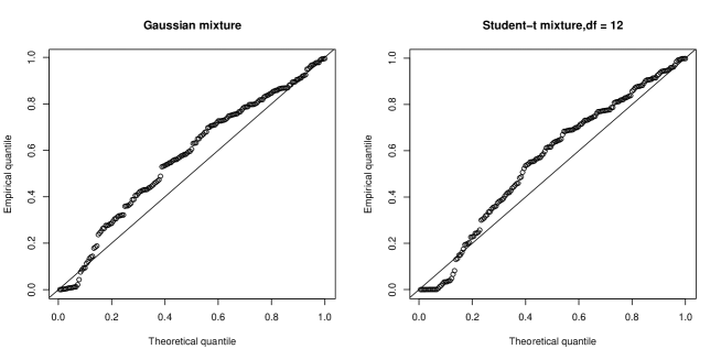
These estimated concordance matrices are very close to their empirical versions and they indicate high longitudinal correlations. To evaluate the goodness-of-fit we implement the modified -plot discussed in Section 6 to the mixture copula models with Negative Binomial marginals in Figure 5. We can see linear trend along the -degree line for both the plots. But for the Student- mixture copula the uniform quantiles are relatively closer to the line than the Gaussian copula. This suggest that Student- mixture copula is more suitable for the temporal dependency for this data set.
8.2 The epilepsy data
We also consider the well-known longitudinal study on epileptic seizures previously analyzed by several authors such as Thall & Vail (1990), Jowaheer & Sutradhar (2002) and Masarotto & Varin (2012) among others. This study was conducted on patients suffering from simple or complex partial seizures. Among these patients, of them were given the anti-epileptic drug progabide and remaining patients were given placebo randomly. The patients were observed for four successive clinical visits after randomization, and the number of seizures occurred over the previous weeks for each individual was reported. Following Ahmmed & Jamee (2021), we consider covariates to analyze this data set as logarithm of baseline seizure count, logarithm of age in years and the treatment indicator ( placebo, progabide). From preliminary descriptive analysis, it is evident that the data is over dispersed. We consider the mean function as
| (8.28) |
where is the respective visit number from to . For this data set also structure seems to be appropriate based on the empirical correlation matrix. We analyze this data set using previously described methodology as well.
| Poisson marginals | Negative Binomial marginals | ||||
|---|---|---|---|---|---|
| Parameters | Est. | SE | Parameters | Est. | SE |
| -3.7090 | 0.9579 | -2.3136 | 0.8877 | ||
| 1.2199 | 0.1543 | 1.0536 | 0.1084 | ||
| -0.0397 | 0.1869 | -0.2421 | 0.1545 | ||
| 0.5184 | 0.2377 | 0.3034 | 0.2312 | ||
| -0.0574 | 0.0350 | -0.0542 | 0.0360 | ||
| - | - | - | 2.6101 | 0.5975 | |
| Model | Copula | Parameters | Est. | SE | Comp-like | CLAIC | CLBIC |
|---|---|---|---|---|---|---|---|
| Poisson | Gaussian | 1.1832 | 0.0875 | -2245.24 | 4636.15 | 4789.72 | |
| exchangeable | |||||||
| Gaussian | 0.5603 | 0.0899 | -2221.13 | 4590.23 | 4743.93 | ||
| mixture | 2.8997 | 0.5365 | |||||
| 0.3485 | 0.0850 | ||||||
| Student- () | 1.2254 | 0.1191 | -2219.88 | 4587.65 | 4742.23 | ||
| exchangeable | |||||||
| Student- () | 0.2496 | 0.4007 | -2219.67 | 4588.32 | 4743.08 | ||
| mixture | 2.7921 | 1.3011 | |||||
| 0.9632 | 0.4314 | ||||||
| Negative | Gaussian | 0.9550 | 0.1141 | -1928.56 | 3889.84 | 3924.25 | |
| Binomial | exchangeable | ||||||
| Gaussian | 0.6836 | 0.1174 | -1919.69 | 3873.65 | 3909.26 | ||
| mixture | 1.4546 | 0.4483 | |||||
| 0.1195 | 0.0799 | ||||||
| Student- () | 0.9172 | 0.1168 | -1924.85 | 3881.29 | 3916.95 | ||
| exchangeable | |||||||
| Student- () | 0.6976 | 0.1244 | -1919.48 | 3872.90 | 3908.15 | ||
| mixture | 1.3930 | 0.4360 | |||||
| 0.1261 | 0.0882 |
The obtained results are reported in Table 7 and 8. As expected from this data set, Negative Binomial based models outperform the Poisson based models and the parameter captured the over dispersion present in the data. The estimate of is negative, which implies patients under the progabide treatment group has lower seizure counts compared to the control group. Based on the estimate of , it shows a positive relation between age and seizure rate. The estimate of shows, the patients who initiated with high seizure rate continued with the same throughout. The estimated standard errors of the marginal parameters are comparably large, which is due to the fact that the sample size is quite low in this data set. Let’s look now to the estimated dependence parameters of the Negative Binomial based models. Student- and Gaussian mixture copula are not significantly different for this data set based on the estimated value of the degrees of freedom parameter and the selection criteria. Interestingly, based on the estimate of , it seems that structure is more prominent, but as we see from relatively high value of , it shows the first component copula is pretty close to the independence copula. As we did previously, we obtain the concordance matrices and compare with their empirical versions for the epilepsy data set. Let , , and be the matrices described in Sub-section 8.1 given as
| (8.37) | ||||
| (8.46) |
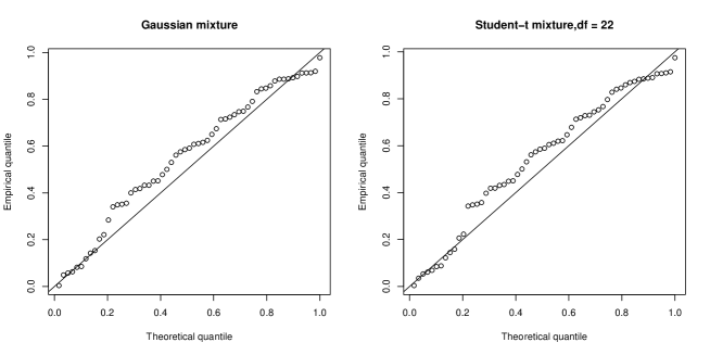
Though the sample size is relatively low for this data set but we see that the best fitting mixture copula closely captured the longitudinal correlation. Finally the modified -plot for the epilepsy data set is given in Figure 6 which shows both of these elliptical mixture copulas captured the temporal dependency similarly. Overall, our models showed substantial improvements to capture the longitudinal correlation than their alternatives. Since we used different covariate setup to analyse these data sets, our parametri results are different than those in Sutradhar (2003) or Jowaheer & Sutradhar (2002) but the conclusions are somewhat similar. However, widely used random effect models can be difficult to interpret and sometimes poses computational challenges in-order to estimate the model parameters due to involvement of multidimensional integrations. Copula based models are in general good alternatives to those, since they can be estimated under efficient one-stage or two-stage estimation procedures with valid standard errors.
9 Discussion
Modeling correlation structure of discrete longitudinal data is an important area of research due to the unavailability of proper multivariate distributions. Nowadays copula approach has become one of the primary techniques to model the dependence structure of multivariate data from various disciplines. Application of copulas in discrete data modeling have not received too much attentions in the literature due to its theoretical limitations. Inspired from the literature of finite mixture models, in this article we introduced mixture of elliptical copulas to model the temporal dependency of longitudinal count data. We derived the dependence properties of finite mixture copulas for continuous and discrete case. Under the full parametric setup we estimated the parameters of our proposed class of models using two stage composite likelihood method and validated through extensive simulation studies. We have also modified and extended the -plot method of model validation for elliptical copulas. Using different correlation structures in each copula components we have shown that our mixture copula models provide better insights to the dependence structure of count longitudinal data. Though we considered balanced case for our analysis, but the approach can be easily extended to the case of unbalanced longitudinal data as long as mixture of elliptical copulas are considered. For simplicity, in this article we considered the number of mixing components to be known. But it will be an interesting to extended to the case when is unknown as described by Yang et al. (2022). One disadvantage of utilizing elliptical copulas is that they can capture symmetric dependence as well as their mixture. We intend to work on this issue in near future.
Acknowledgments:
Author is grateful to Prof. Sumitra Purkayastha of Applied Statistics Unit, ISI Kolkata for some helpful discussions.
References
- (1)
- Ahmmed & Jamee (2021) Ahmmed, F. & Jamee, A. R. (2021), ‘Generalized quasi-likelihood estimation procedure for non-stationary over-dispersed longitudinal counts’, Journal of Statistical Computation and Simulation 91(9), 1802–1814.
- Arakelian & Karlis (2014) Arakelian, V. & Karlis, D. (2014), ‘Clustering dependencies via mixtures of copulas’, Communications in Statistics-Simulation and Computation 43(7), 1644–1661.
- Böhning (1999) Böhning, D. (1999), Computer-assisted analysis of mixtures and applications: meta-analysis, disease mapping and others, Vol. 81, CRC press.
- Demarta & McNeil (2005) Demarta, S. & McNeil, A. J. (2005), ‘The t copula and related copulas’, International statistical review 73(1), 111–129.
- Denuit & Lambert (2005) Denuit, M. & Lambert, P. (2005), ‘Constraints on concordance measures in bivariate discrete data’, Journal of Multivariate Analysis 93(1), 40–57.
- Diao & Cook (2014) Diao, L. & Cook, R. J. (2014), ‘Composite likelihood for joint analysis of multiple multistate processes via copulas’, Biostatistics 15(4), 690–705.
- Frahm et al. (2003) Frahm, G., Junker, M. & Szimayer, A. (2003), ‘Elliptical copulas: applicability and limitations’, Statistics & Probability Letters 63(3), 275–286.
- Frees & Wang (2006) Frees, E. W. & Wang, P. (2006), ‘Copula credibility for aggregate loss models’, Insurance: Mathematics and Economics 38(2), 360–373.
- Frühwirth-Schnatter (2006) Frühwirth-Schnatter, S. (2006), Finite mixture and Markov switching models, Vol. 1, Springer.
- Gao & Song (2010) Gao, X. & Song, P. X.-K. (2010), ‘Composite likelihood bayesian information criteria for model selection in high-dimensional data’, Journal of the American Statistical Association 105(492), 1531–1540.
- Genest & Nešlehová (2007) Genest, C. & Nešlehová, J. (2007), ‘A primer on copulas for count data’, ASTIN Bulletin: The Journal of the IAA 37(2), 475–515.
- Genest et al. (2009) Genest, C., Rémillard, B. & Beaudoin, D. (2009), ‘Goodness-of-fit tests for copulas: A review and a power study’, Insurance: Mathematics and economics 44(2), 199–213.
- Gibbons et al. (2010) Gibbons, R. D., Hedeker, D. & DuToit, S. (2010), ‘Advances in analysis of longitudinal data’, Annual review of clinical psychology 6, 79–107.
- Holzmann et al. (2006) Holzmann, H., Munk, A. & Gneiting, T. (2006), ‘Identifiability of finite mixtures of elliptical distributions’, Scandinavian journal of statistics 33(4), 753–763.
- Jaworski et al. (2010) Jaworski, P., Durante, F., Hardle, W. K. & Rychlik, T. (2010), Copula theory and its applications, Vol. 198, Springer.
- Joe (1990) Joe, H. (1990), ‘Multivariate concordance’, Journal of multivariate analysis 35(1), 12–30.
- Joe (2014) Joe, H. (2014), Dependence modeling with copulas, 1 edn, Chapman and Hall/CRC.
- Jowaheer & Sutradhar (2002) Jowaheer, V. & Sutradhar, B. C. (2002), ‘Analysing longitudinal count data with overdispersion’, Biometrika 89(2), 389–399.
- Karlis (2019) Karlis, D. (2019), ‘Mixture modelling of discrete data’, Handbook of Mixture Analysis 1, 193–218.
- Ko & Hjort (2019) Ko, V. & Hjort, N. L. (2019), ‘Copula information criterion for model selection with two-stage maximum likelihood estimation’, Econometrics and Statistics 12, 167–180.
- Kosmidis & Karlis (2016) Kosmidis, I. & Karlis, D. (2016), ‘Model-based clustering using copulas with applications’, Statistics and computing 26, 1079–1099.
- le Cessie & Van Houwelingen (1994) le Cessie, S. & Van Houwelingen, J. (1994), ‘Logistic regression for correlated binary data’, Journal of the Royal Statistical Society: Series C 43(1), 95–108.
- Li et al. (1997) Li, R.-Z., Fang, K.-T. & Zhu, L.-X. (1997), ‘Some qq probability plots to test spherical and elliptical symmetry’, Journal of Computational and Graphical Statistics 6(4), 435–450.
- Liu et al. (2023) Liu, Y., Xie, D., Edwards, D. A. & Yu, S. (2023), ‘Mixture copulas with discrete margins and their application to imbalanced data’, Journal of the Korean Statistical Society 52(4), 878–900.
- MacDonald (2014) MacDonald, I. L. (2014), ‘Numerical maximisation of likelihood: A neglected alternative to em?’, International Statistical Review 82(2), 296–308.
- Madsen & Fang (2011) Madsen, L. & Fang, Y. (2011), ‘Joint regression analysis for discrete longitudinal data’, Biometrics 67(3), 1171–1175.
- Masarotto & Varin (2012) Masarotto, G. & Varin, C. (2012), ‘Gaussian copula marginal regression’, Electronic Journal of Statistics 6, 1517 – 1549.
- McLachlan et al. (2019) McLachlan, G. J., Lee, S. X. & Rathnayake, S. I. (2019), ‘Finite mixture models’, Annual review of statistics and its application 6, 355–378.
- Mesfioui & Tajar (2005) Mesfioui, M. & Tajar, A. (2005), ‘On the properties of some nonparametric concordance measures in the discrete case’, Nonparametric Statistics 17(5), 541–554.
- Nelsen (2002) Nelsen, R. B. (2002), ‘Concordance and copulas: A survey’, Distributions with given marginals and statistical modelling pp. 169–177.
- Nelsen (2006) Nelsen, R. B. (2006), An introduction to copulas, 2 edn, Springer.
- Nikoloulopoulos & Karlis (2009) Nikoloulopoulos, A. K. & Karlis, D. (2009), ‘Modeling multivariate count data using copulas’, Communications in Statistics-Simulation and Computation 39(1), 172–187.
- Nikoloulopoulos & Karlis (2010) Nikoloulopoulos, A. K. & Karlis, D. (2010), ‘Regression in a copula model for bivariate count data’, Journal of Applied Statistics 37(9), 1555–1568.
- Peel & McLachlan (2000) Peel, D. & McLachlan, G. J. (2000), ‘Robust mixture modelling using the t distribution’, Statistics and computing 10, 339–348.
- Safari-Katesari et al. (2020) Safari-Katesari, H., Samadi, S. Y. & Zaroudi, S. (2020), ‘Modelling count data via copulas’, Statistics 54(6), 1329–1355.
- Shi (2012) Shi, P. (2012), ‘Multivariate longitudinal modeling of insurance company expenses’, Insurance: Mathematics and Economics 51(1), 204–215.
- Shi et al. (2016) Shi, P., Feng, X. & Boucher, J.-P. (2016), ‘Multilevel modeling of insurance claims using copulas’.
- Shi & Valdez (2014) Shi, P. & Valdez, E. A. (2014), ‘Longitudinal modeling of insurance claim counts using jitters’, Scandinavian Actuarial Journal 2014(2), 159–179.
- Song et al. (2009) Song, P. X.-K., Li, M. & Yuan, Y. (2009), ‘Joint regression analysis of correlated data using gaussian copulas’, Biometrics 65(1), 60–68.
- Sun et al. (2008) Sun, J., Frees, E. W. & Rosenberg, M. A. (2008), ‘Heavy-tailed longitudinal data modeling using copulas’, Insurance: Mathematics and Economics 42(2), 817–830.
- Sutradhar (2003) Sutradhar, B. C. (2003), ‘An overview on regression models for discrete longitudinal responses’, Statistical science 18(3), 377–393.
- Sutradhar (2011) Sutradhar, B. C. (2011), Dynamic mixed models for familial longitudinal data, Vol. 18, Springer.
- Teicher (1963) Teicher, H. (1963), ‘Identifiability of finite mixtures’, The annals of Mathematical statistics pp. 1265–1269.
- Thall & Vail (1990) Thall, P. F. & Vail, S. C. (1990), ‘Some covariance models for longitudinal count data with overdispersion’, Biometrics pp. 657–671.
- Titterington et al. (1985) Titterington, D. M., Smith, A. F. & Makov, U. E. (1985), ‘Statistical analysis of finite mixture distributions’, (No Title) .
- Varin & Czado (2010) Varin, C. & Czado, C. (2010), ‘A mixed autoregressive probit model for ordinal longitudinal data’, Biostatistics 11(1), 127–138.
- Varin et al. (2011) Varin, C., Reid, N. & Firth, D. (2011), ‘An overview of composite likelihood methods’, Statistica Sinica pp. 5–42.
- Varin & Vidoni (2005) Varin, C. & Vidoni, P. (2005), ‘A note on composite likelihood inference and model selection’, Biometrika 92(3), 519–528.
- Weiss (2005) Weiss, R. E. (2005), Modeling longitudinal data, Vol. 1, Springer, USA.
- Xu et al. (2007) Xu, S., Jones, R. H. & Grunwald, G. K. (2007), ‘Analysis of longitudinal count data with serial correlation’, Biometrical Journal: Journal of Mathematical Methods in Biosciences 49(3), 416–428.
- Xue-Kun Song (2000) Xue-Kun Song, P. (2000), ‘Multivariate dispersion models generated from gaussian copula’, Scandinavian Journal of Statistics 27(2), 305–320.
- Yakowitz & Spragins (1968) Yakowitz, S. J. & Spragins, J. D. (1968), ‘On the identifiability of finite mixtures’, The Annals of Mathematical Statistics 39(1), 209–214.
- Yang et al. (2022) Yang, B., Cai, Z., Hafner, C. M. & Liu, G. (2022), ‘Time-varying mixture copula models with copula selection’, Statistica Sinica 32(2), 1049–1077.
- Zhao & Joe (2005) Zhao, Y. & Joe, H. (2005), ‘Composite likelihood estimation in multivariate data analysis’, Canadian Journal of Statistics 33(3), 335–356.
- Zhuang et al. (2022) Zhuang, H., Diao, L. & Grace, Y. Y. (2022), ‘A bayesian nonparametric mixture model for grouping dependence structures and selecting copula functions’, Econometrics and Statistics 22, 172–189.
Appendix A Appendix
Here we present the proofs of the theorems stated in Section 3.
Proof of Theorem 3.1:
Let be an independent copy of . Using the definition of Kendall’s tau we have -
| (A.1) |
Since , by plugging the values in equation (A) we obtain the result.
Proof of Theorem 3.2:
Let be two independent random variables (i.e. bivariate random vector with independence copula) with same marginal distributions . Using the definition of Spearman’s rho we have -
| (A.2) |
Since , by plugging the values in equation (A) we obtain the result.
Proof of Theorem 3.3:
When is integer valued random vector the probability of tie is non-zero and . Therefore we have -
| (A.3) |
The last expression is due to the fact that and are identically distributed.
| (A.4) |
| (A.5) |
Therefore, using (A) and (A) in (A) we get -
since , and hence the proof is completed.
Proof of Theorem 3.4:
Using the same definition we have -
| (A.6) |
The last expression is due to the fact that and have different joint distribution.
| (A.7) |
| (A.8) |
| (A.9) |
Therefore, using (A), (A) and (A) in (A) we get -
and hence the proof is completed.
Proof of Theorem 3.5:
Straight from the definition we have -