Sun-Jupiter-Saturn system may exist: a verified computation of quasiperiodic solutions for the planar three body problem

Abstract.

In this paper, we present evidence of the stability of a simplified model of the Solar System, a flat (Newtonian) Sun-Jupiter-Saturn system with realistic data: masses of the Sun and the planets, their semi-axes, eccentricities and (apsidal) precessions of the planets close to the real ones. The evidence is based on convincing numerics that a KAM theorem can be applied to the Hamiltonian equations of the model to produce quasiperiodic motion (on an invariant torus) with the appropriate frequencies. To do so, we first use KAM numerical schemes to compute translated tori to continue from the Kepler approximation (two uncoupled two-body problems) up to the actual Hamiltonian of the system, for which the translated torus is an invariant torus. Second, we use KAM numerical schemes for invariant tori to refine the solution giving the desired torus. Lastly, the convergence of the KAM scheme for the invariant torus is (numerically) checked by applying several times a KAM iterative lemma, from which we obtain that the final torus (numerically) satisfies the existence conditions given by a KAM theorem.

1. Introduction

In [40] Newton deduced the equations for the motion of planets and solved the 2 body problem: bounded orbits follow Kepler’s motions (spin in ellipses with one focus on the center of mass), and unbounded ones are parabolae or hyperbolae. Then Newton (Book 3, Proposition XIII, Theorem XIII) admits that observed planetary motion Jupiter does not fit the equations, and explains it by noticing that Saturn’s influence can not be neglected. Since then, one of the most important problems in mathematics has been understanding the dynamics of the 3 (or higher) body problem. Many researchers have pursued this question and realized in different temporal stages that there are two (among others) important questions: the stability of the solutions - do planets orbit around the Sun in a quasiperiodic motion ad perpetuum? -; and the existence of chaos. This dichotomy was started by the pioneer work of Poincaré in [41]. In this paper we are interested in the stability problem.

Several steps forward in time and we encounter a fundamental advance towards solving the stability problem. In 1954 Kolmogorov [31] presented a methodology for proving the existence of Lagrangian invariant tori in Hamiltonian systems of $n$ degrees of freedom close to integrable ones. Then Arnold [4, 5] and Moser [38] further explored this and the KAM theory was officially born. Since then a lot results have been produced, covering Lagrangian and lower dimensional tori, infinite dimensional systems, dissipative systems, etc. For the interested reader, we refer to the books [6, 14, 11], and the popular book [16].

It was clear from the very beginning that the 3 body problem posed several obstacles that other Hamiltonians don’t have. The integrable problem (Kepler’s Hamiltonian) doesn’t have all the frequencies that the full problem has: in a general four degrees of freedom Hamiltonian invariant tori have four dimensions with four frequencies; while in Kepler’s Hamiltonian they have two dimensions with two frequencies. In KAM terminology it is said that the system is degenerate, and then the full problem has several time-scale frequencies: the fast frequencies that correspond to the spinning of the planets around the Sun, and the slow frequencies that correspond to the spinning of their orbital ellipses (precession motion) and, in the spatial problem, the changes in the inclination of the rotation planes (inclination motion).

A crucial advance was performed by Arnold in [3, 5] where he proved the persistence of quasiperiodic motion for the planar three body problem for a ratio of the semi-major axis close to zero. The theory was later completed for the spatial $N$ body problem in remarkable works by Herman and Féjoz [17], and Chierchia and Pinzari [12], among others. In spite of the fundamental importance of all these theoretical results, they suffer the practical inconvenience that the ratio of the semi-major axis or the size of masses of the planets (used as the parameter measuring the distance to integrability) have to be ridiculously small. In fact, Hénon [29] already took Arnold’s paper and checked that this size, in the simpler and non-degenerate restricted three body problem, is of order $10^{-333}$ (see the beautiful exposition of these facts in [33]). After this result Hénon asserted : “Thus, these theorems, although of a very great theoretical interest, do not seem applicable in their present state to practical problems, where the perturbations are always much larger than the thresholds [above].” This apparent lack of applicability of KAM theory to practical and physical problems led over time to some misunderstandings (and laugther) about KAM theory but, as Dumas emphasizes in [16], Hénon himself goes on to write: “The numerical results we present here, and those obtained for other problems, indicate however that the [invariant] curves continue to exist for very strong perturbations, of the same order of magnitude as the leading term.”

This last observation by Hénon is in fact what leads our research: the combination of qualitative KAM results with computers. The idea is the use of the computers for getting initial data that can be then checked to fulfill the conditions of the taylored KAM theorems. Following this line of thought in combination with all the previous (classical) KAM methodology, based on performing canonical transformations on the Hamiltonian, there has been important advancement towards the solution of the three body problem for realistic masses [34, 43, 35, 36, 9]. More recently, in [8] a quantitative version of Arnold’s KAM theorem have been applied to the plane three-body problem to show, computer-assisted, the existence of quasiperiodic motion for a ratio of masses between the planets and the star that is close to $10^{-85}$ (this estimate accounts for a mass of the planets smaller than $10^{-24}$ times the mass of the electron). In this paper, however, we propose to use another approach, based on the so-called parameterization method (see the seminal works [14, 15]), looking directly for the parameterizations of the invariant tori, mitigating the curse of dimensionality. In this approach, the KAM theorems are written in a posteriori format, so that the results are suitable for numerical verification and, finally, for Computer-Assisted Proofs. This program has led to a rapid development of results [27, 21, 28, 22, 7].

Applying KAM theory to the planar three body problem (for realistic parameters and ephemerides) is a very demanding problem, both mathematically and computationally. Hence, further steps must be performed to attack the problem. We have split this enterprise in three stages, of which the present paper is the centerpiece. Each stage deals with different questions and methods, so they could be of independent interest for different publics. Moreover, even though we have been thinking in the application to the three body problem, and specifically to the Sun-Jupiter-Saturn system, the pieces can be applied to other problems. The first stage, appearing in [20], is a KAM theorem based on a (modified) parameterization method for Hamiltonian systems, with sharp control on the bounds and the Diophantine frequencies (with precedents in [28, 44]). This first paper has two results that we use in this paper: the KAM Theorem for verifying the existence of the invariant torus, and the Iterative Lemma used for, giving an initial approximation with bounds on it, we perform several steps of the convergence scheme. This allows to refine the constants to be used later on the KAM Theorem. The second stage, this paper, is a methodology to compute invariant tori in (close to degenerate) Hamiltonian systems with fast and slow time-scales, applied to numerically verify the existence of quasiperiodic solutions of the Sun-Jupiter-Saturn in the planar model with realistic masses and ephemerides. The last stage is [19] where we present how the numerics from this paper and the KAM theorem from [20] are combined along with rigorous numerics for validating the results.

1.1. Our results and their organization in the paper

We start presenting the model we work on. It is a Hamiltonian with 3 degrees of freedom (the total angular momentum has been reduced) depending on a parameter $\mu$ that accounts for the masses, so that $\mu=0$ corresponds to two uncoupled Kepler problems, and $\mu=\mu_{0}$ corresponds to the actual values of the masses of the planets (in our case $\mu_{0}=10^{-3}$). Then we discuss the numerical methods used. The goal is computing a 3 dimensional invariant torus for the observed values of the frequencies (for $\mu=\mu_{0}$). Two of the frequencies are fast, and the other is slow and of the order of $\mu_{0}$. A fundamental obstacle we encounter is that the torus does not come by continuation from a 3 dimensional invariant torus for $\mu=0$, because Kepler motions correspond to 2 dimensional tori, and the slow frequency collapses to zero. Hence, we cannot apply a direct continuation technique of the invariant tori from the integrable problem since the problem is singular at $\mu=0$. Following the lines of thought of [25, 26] we perform a continuation of translated tori, which are invariant tori for a modified Hamiltonian system to which we have added an extra term (a translation) that compensates the degeneracies of the actual problem. At $\mu=\mu_{0}$, the translation term should be zero. At this stage the torus is no longer degenerate, allowing the use of KAM numerical schemes on the actual problem for its refinement. This leads to, after iterating several times the KAM numerical scheme, obtaining a very accurate approximation for the invariant torus. Finally, with this approximation, we can run the Iterative Lemma in [20] several times and, lastly, the KAM Theorem so that all the bounds satisfy it and gives us the the existence of a nearby invariant torus, hence giving a numerical verification of the existence of quasiperiodic solutions close to the ephemerides of Sun-Jupiter-Saturn configuration. Paraphrasing Henón, the numerical results we present here indicate that the invariant torus exists for $\mu=\mu_{0}$.

2. The planetary model and the problem

The planar $(1+{n})$-body problem (the Sun plus ${n}$ planets) in Poincaré heliocentric cartesian coordinates has Hamiltonian [34, 12] $H_{\rm C}:{\mathbb{R}}^{2n}\times{\mathbb{R}}^{2n}\rightarrow{\mathbb{R}}$ given by

(2.1) $$\begin{split}H_{\rm C}(x,y)&=\sum_{i=1}^{n}\left(\dfrac{\|y_{i}\|^{2}}{2m_{i}}-\dfrac{m_{i}}{\|x_{i}\|}\right)+\mu\left(\sum_{i=1}^{n}\dfrac{\|y_{i}\|^{2}}{2}+\sum_{1\leq i<j\leq{n}}\left(y_{i}\cdot y_{j}-\dfrac{m_{i}m_{j}}{\|x_{i}-x_{j}\|}\right)\right)\\ &=H_{\rm C}^{0}(x,y)+\mu\ H_{\rm C}^{1}(x,y),\end{split}$$

where the $0$-th body (the Sun) has mass $1$ and is fixed at the origin and the $i$-th body has mass $\mu m_{i}$ and position-momentum coordinates ${(x_{i},y_{i})=(x_{i,1},x_{i,2},y_{i,1},y_{i,2})}$. Also, the length and time units are chosen so that the gravitational constant is $1$ and the period of an elliptical orbit of semi-major axis $1$ is $2\pi$ (so its frequency is $1$, and this the case of the Earth in the Solar system).

The $\mu=0$ case corresponds to the integrable Keplerian motion of the planets around the Sun (no interaction between planets). Well-known angle-action coordinates for the Keplerian motion are Delaunay coordinates. These are defined body-wise: The Delaunay coordinates of the $i$-th body are $(\ell_{i},g_{i},L_{i},G_{i})\in{\mathbb{T}}^{2}\times{\mathbb{R}}^{2}$, with $G_{i}<L_{i}$ and ${\mathbb{T}}={\mathbb{R}}/{2\pi{\mathbb{Z}}}$, are mapped to the Cartesian coordinates $(x_{i,1},x_{i,2},y_{i,1},y_{i,2})\in{\mathbb{R}}^{4}$ through the following steps:

$$e_{i}=\sqrt{1-\left(\frac{G_{i}}{L_{i}}\right)^{2}},\ a_{i}=\dfrac{(L_{i})^{2}}{m_{i}^{2}},\ b_{i}=\dfrac{m_{i}^{2}}{L_{i}},\ E_{i}=K(\ell_{i},e_{i}),$$

$$\begin{pmatrix}q_{i,1}\\ q_{i,2}\end{pmatrix}=a_{i}\begin{pmatrix}\cos(E_{i})-e_{i}\\ \dfrac{G_{i}}{L_{i}}\sin(E_{i})\end{pmatrix},\qquad\begin{pmatrix}x_{i,1}\\ x_{i,2}\end{pmatrix}=\begin{pmatrix}\cos(g_{i})&-\sin(g_{i})\\ \sin(g_{i})&\cos(g_{i})\end{pmatrix}\begin{pmatrix}q_{i,1}\\ q_{i,2}\end{pmatrix}$$

$$\begin{pmatrix}p_{i,1}\\ p_{i,2}\end{pmatrix}=\dfrac{b_{i}}{1-e_{i}\cos(E_{i})}\begin{pmatrix}-\sin(E_{i})\\ \dfrac{G_{i}}{L_{i}}\cos(E_{i})\end{pmatrix},\qquad\begin{pmatrix}y_{i,1}\\ y_{i,2}\end{pmatrix}=\begin{pmatrix}\cos(g_{i})&-\sin(g_{i})\\ \sin(g_{i})&\cos(g_{i})\end{pmatrix}\begin{pmatrix}p_{i,1}\\ p_{i,2}\end{pmatrix}$$

where $E=K(\ell,e)$ denotes the solution of the Kepler equation $\ell=E-e\sin(E)$.

The Hamiltonian (2.1) is then written in Delaunay coordinates $(\ell,g,L,G)$ as a function $H_{\rm D}:{\mathbb{T}}^{2n}\times{\mathbb{R}}^{2n}\rightarrow{\mathbb{R}}$ given by

$$\begin{split}H_{\rm D}(\ell,g,L,G)&=\sum_{i=1}^{n}\frac{-m_{i}^{3}}{2L_{i}^{2}}+\mu\ H_{\rm C}^{1}{\!\>\circ\!\,}D(\ell,g,L,G)=H_{\rm D}^{0}(L)+\mu\ H_{\rm D}^{1}(\ell,g,L,G),\\ \end{split}$$

where $D$ denotes the Delaunay map from Delaunay coordinates $(\ell,g,L,G)$ to Cartesian coordinates $(x,y)$ described above.

Let us denote by $\hat{G}_{i}=\sum_{1\leq k\leq i}G_{k}$ the angular momentum of the $i$ first planets. It is well-known that the total angular momentum, $\hat{G}_{n}$, is a first integral of the Hamiltonian system, so that we can reduce by one the number of degrees of freedom by fixing the value $\hat{G}_{n}=\hat{G}_{{n},0}$. By extending the angular momentum map above to a canonical transformation, taking $\hat{g}_{i}=g_{i}-g_{i+1}$ for $i=1,\dots,{n}-1$, and $\hat{g}_{n}=g_{n}$, one gets that $\hat{g}_{n}$ is a cyclic coordinate in the transformed Hamiltonian in the new coordinates. Hence, by fixing the total angular momentum $\hat{G}_{n}$ to a given value $\hat{G}_{{n},0}$, one gets a reduced Hamiltonian ${H_{\hat{G}_{{n},0}}:{\mathbb{T}}^{2n-1}\times{\mathbb{R}}^{2{n}-1}\rightarrow{\mathbb{R}}}$ given by

(2.2) $$H_{\hat{G}_{{n},0}}(\ell,\hat{g},L,\hat{G})=H_{\rm D}^{0}(L)+\mu H^{1}_{\hat{G}_{{n},0}}(\ell,\hat{g},{{{\mbox{\rm D}}{K}}},\hat{G}),$$

with $\hat{g}=(\hat{g}_{1},\dots,\hat{g}_{{n}-1})$ and $\hat{G}=(\hat{G}_{1},\dots,\hat{G}_{{n}-1})$. From now on, we will omit the dependence on $\hat{G}_{{n},0}$ from the notation.

A Lagrangian invariant torus of $H$, with a $(2{n}-1)$-dimensional vector of frequencies $(\omega^{\ell},\omega^{\hat{g}})\in{\mathbb{R}}^{n}\times{\mathbb{R}}^{{n}-1}$ and total angular momentum $\hat{G}_{{n},0}$, gives raise to a Lagrangian invariant torus of $H_{\rm D}$, with a $2{n}$-dimensional vector of frequecies $(\omega^{\ell},\omega^{g})\in{\mathbb{R}}^{n}\times{\mathbb{R}}^{{n}}$ (see Reduction Lemma in [20]). The frequencies are related by $\omega_{i}^{\hat{g}}=\omega_{i}^{g}-\omega_{i+1}^{g}$ for $i=1,\dots n-1$, and $\omega_{n}^{\hat{g}}=\omega_{n}^{g}$ is the average of $\frac{\partial H}{\partial\hat{G}_{{n}}}$ over the $(2{n}-1)$-dimensional invariant torus. We emphasize that $\omega^{\ell}$ contains the fast frequencies (the ones coming from the Keplerian motion), and that $\omega^{\hat{g}}$ (or $\omega^{g}$) contains the slow frequencies (that in our case are proportional to $\mu$). This smallness is a main difficulty when facing the $(1+{n})$-body problem with realistic data (big masses and no big axes).

2.1. Invariance equation

In the light of the parameterization method, finding invariant tori for $H$ with frequency vector $\omega=(\omega^{\ell},\omega^{\hat{g}})$ reduces to finding a parameterization of the torus ${K:{\mathbb{T}}^{2{n}-1}\rightarrow{\mathbb{T}}^{2{n}-1}\times{\mathbb{R}}^{2{n}-1}}$ satisfying the invariant torus equation

(2.3) $${\mathfrak{L}_{\omega}}K(\theta)+X_{H}(K(\theta))=0,$$

where $\mathfrak{L}_{\omega}$ is a Lie operator acting on any smooth function $f:{\mathbb{T}}^{2{n}-1}\rightarrow{\mathbb{R}}^{M}$ by ${{\mathfrak{L}_{\omega}}f(\theta)=-{\rm D}f(\theta)\omega,}$ and $X_{H}=\Omega^{-1}({\rm D}H)^{\top}$ is the Hamiltonian vector field with respect to the standard symplectic form given by the matrix

$$\Omega=\begin{pmatrix}O&-I\\ I&O\end{pmatrix}.$$

We write $J=\Omega$ when we think of such a matrix as a linear map instead of as a 2-form. In particular, we use $J$ to define a normal bundle to the torus parameterized by $K$, framed by the columns of $N(\theta)=J{\mbox{\rm D}}K(\theta)({\mbox{\rm D}}K(\theta)^{\top}{\mbox{\rm D}}K(\theta))^{-1}$, where the columns of ${\mbox{\rm D}}K(\theta)$ frame the tangent bundle. Moreover, the symmetric matrix

$$T(\theta)=N(\theta)^{\top}\Omega({\mbox{\rm D}}X_{H}(K(\theta))+J{\mbox{\rm D}}X_{H}(K(\theta))J)N(\theta)$$

measures how much the normal bundle is twisted (the tangent bundle of an invariant torus is fixed). The non-degeneracy of the average of $T$, the torsion, plays the role of the classical Kolmogorov non-degeneracy condition in KAM theory.

As it is also costumary in KAM theory, we assume that $\omega$ is Diophantine, i.e. there exists $\gamma>0$ and $\tau\geq 2{n}-2$ such that for any $k\in{\mathbb{Z}}^{2{n}-1}$ and $k\neq 0$, $|k\cdot\omega|\geq\gamma|k|_{1}^{-\tau}$. Given any real-analytic function $s:{\mathbb{T}}^{2{n}-1}\rightarrow{\mathbb{R}}^{M}$, we denote by ${\mathfrak{R}_{\omega}}(s)$ the only real-analytic function $f:{\mathbb{T}}^{2{n}-1}\rightarrow{\mathbb{R}}^{M}$, with average zero, that satisfies ${\mathfrak{L}_{\omega}}f=s-\langle{s}\rangle$, where $\langle{s}\rangle$ denotes the average of the function $s$. This operator is in the core of KAM theory.

3. Continuation from the integrable case with translated tori methods

Notice that for $\mu=0$ the reduced Hamiltonian (2.2) has the invariant tori

(3.1) $$K_{\hat{G}_{0}}(\theta^{\ell},\theta^{\hat{g}})=(\theta^{\ell},\theta^{\hat{g}},L_{0},{\hat{G}_{0}})$$

where the components of $L_{0}$ are determined by the masses of the bodies and the fast frequencies $\omega^{\ell}$ (by the third Kepler’s law), but the secular frequency $\omega^{\hat{g}}_{0}$ is zero (not $\omega^{\hat{g}}$!) and $\hat{G}_{0}$ is free: there is an $({n}-1)-$parameter family of $(2{n}-1)$-dimensional tori foliated by ${n}$-dimensional invariant tori. As a result, the torsion is noninvertible (since there is no twist in the $\hat{G}$ direction). In summary: the problem is degenerate.

3.1. A translated torus algorithm

As mentioned above, the degeneracy of the problem imposes a first obstacle for applying any numerical KAM scheme for performing any continuation with respect to $\mu$. In the spirit of [25, 26], we can overcome this degeneracy by introducing a counterterm $\lambda\,\Pi_{\hat{G}}$ to the Hamiltonian (2.2), where $\Pi_{\hat{G}}:{\mathbb{T}}^{2n-1}\times{\mathbb{R}}^{2n-1}\rightarrow{\mathbb{R}}$ is the projection onto the $\hat{G}$ coordinate. Hence, by denoting $X_{\hat{G}}=X_{\Pi_{\hat{G}}}$, instead of solving Equation (2.3), we solve the extended system

(3.2) $$\left\{\begin{split}\mathfrak{L}_{\omega}K(\theta)+X_{H}(K(\theta))+X_{\hat{G}}(K(\theta))\lambda&=0,\\ \langle{\Pi_{\hat{G}}(K(\theta))}\rangle-\hat{G}_{0}&=0,\end{split}\right.$$

for a fixed constant $\hat{G}_{0}$. The invariant tori satisfying (3.2) are translated tori for the original Hamiltonian system. Since $\hat{G}_{0}$ is an extra parameter, under appropriate non-degeneracy conditions (that we will see later are very mild), we can find families of translated tori, labeled by $\hat{G}_{0}$. The use of counterterms in KAM theory goes back to the works of Moser and Herman [39, 30, 17, 18].

Notice that, for a given $\hat{G}_{0}$, for $\mu=0$ the parameterization (3.1) satisfies (3.2) with frequency $\omega=(\omega^{\ell},\omega^{\hat{g}})$, by selecting $\lambda=\omega^{\hat{g}}$. The idea is then performing a continuation method for solving the translated torus equation (3.2) for couples $(K,\lambda)$ up to the value $\mu=\mu_{0}$. The rationale behing this method is that, if there were an invariant torus with frequency $\omega=(\omega^{\ell},\omega^{\hat{g}})$ and $\langle{\Pi_{\hat{G}}{\!\>\circ\!\,}K}\rangle=\hat{G}_{0}$ for $\mu=\mu_{0}$, then after the continuation procedure we would find $(K,\lambda)$ with $\lambda=0$. Using perturbation theory up to order one (expanding in Poincaré-Lindsedt series) we get an approximation of $\hat{G}_{0}$ by solving the equation $\langle{\Pi_{\hat{g}}X_{H^{1}}\circ K_{\hat{G}}}\rangle=\omega^{\hat{g}}/\mu_{0},$ where $\Pi_{\hat{g}}$ is the projection onto the $\hat{g}$ component. We then continue this solution from $\mu=0$ to $\mu=\mu_{0}$ by solving the equations at each step, see Subsection 3.1.1. Finally, since this value of $\hat{G}_{0}$ is not exact, we don’t get $\lambda=0$ at $\mu=\mu_{0}$. However, at $\mu_{0}$ on can also tune $\hat{G}_{0}$ to get $\lambda=0$ by a Newton method (again using perturbation methods for computing $\frac{\partial\lambda}{\partial\hat{G}_{0}}$). .

3.1.1. Solving Equations (3.2)

More concretetly, from an approximate solution $(K(\theta),\lambda)$ of (3.2) we can perform a quasi-Newton correction of the form $(P(\theta)\xi(\theta),\Delta\lambda)$, where the matrix $P(\theta)=\begin{pmatrix}{\mbox{\rm D}}K(\theta)&N(\theta))\end{pmatrix}$, obtained by yuxtaposing the tangent and normal frames given above, is approximately symplectic. Taking into account that the inverse of $P(\theta)$ is close to $-\Omega P(\theta)^{T}\Omega$, we end up with the linear system

$$\left\{\begin{split}{\mathfrak{L}_{\omega}}\xi^{{\rm D}\!{K}}(\theta)+T(\theta)\xi^{N}(\theta)+b^{{\rm D}\!K}(\theta)\Delta\lambda&=\eta^{{\rm D}\!K}(\theta),\\ {\mathfrak{L}_{\omega}}\xi^{N}(\theta)+\phantom{T(\theta)\xi^{N}(\theta)+}b^{N}(\theta)\Delta\lambda&=\eta^{N}(\theta),\\ \langle{\Pi_{\hat{G}}({\mbox{\rm D}}K(\theta)\xi^{{\rm D}\!{K}}(\theta)+N(\theta)\xi^{N}(\theta))}\rangle&=\eta^{\hat{G}_{0}},\end{split}\right.$$

where $\begin{pmatrix}b^{{\rm D}\!K}(\theta)\\ b^{N}(\theta)\end{pmatrix}=\begin{pmatrix}N(\theta)^{\top}\\ -{{\mbox{\rm D}}{K}}(\theta)^{\top}\end{pmatrix}\Omega X_{\hat{G}}(K(\theta))$, $\begin{pmatrix}\eta^{{\rm D}\!K}(\theta)\\ \eta^{N}(\theta)\end{pmatrix}=\begin{pmatrix}-N(\theta)^{\top}\\ {{\mbox{\rm D}}{K}}(\theta)^{\top}\end{pmatrix}\Omega(\mathfrak{L}_{\omega}K(\theta)+X_{H}(K(\theta))+\lambda X_{\hat{G}}(K(\theta)))$, $\eta^{\hat{G}_{0}}=-\langle{\Pi_{\hat{G}}\circ K}\rangle+\hat{G}_{0}$.

As it is customary in these types of schemes, one solves them up to some a-priori unknowns: In this case the average $\xi^{N}_{0}=\langle{\xi^{N}}\rangle$ and $\Delta\lambda$. These two satisfy the linear system

(3.3) $$\begin{pmatrix}\langle{T}\rangle&\langle{{\tilde{b}}^{{\rm D}\!K}}\rangle\\ \langle{\Pi_{\hat{G}}(N-DK{\mathfrak{R}_{\omega}}T)}\rangle&-\langle{\Pi_{\hat{G}}(DK{\mathfrak{R}_{\omega}}{\tilde{b}}^{{\rm D}\!K}+N{\mathfrak{R}_{\omega}}b^{N})}\rangle\end{pmatrix}\begin{pmatrix}\xi^{N}_{0}\\ \Delta\lambda\end{pmatrix}=\begin{pmatrix}\langle{{\tilde{\eta}}^{{\rm D}\!K}}\rangle\\ \eta^{\hat{G}_{0}}-\langle{\Pi_{\hat{G}}{\mbox{\rm D}}K{\mathfrak{R}_{\omega}}{\tilde{\eta}}^{{\rm D}\!K}}\rangle\end{pmatrix},$$

where ${\tilde{b}}^{{\rm D}\!K}=b^{{\rm D}\!K}-T{\mathfrak{R}_{\omega}}b^{N}$ and ${\tilde{\eta}}^{{\rm D}\!K}=\eta^{{\rm D}\!K}-T{\mathfrak{R}_{\omega}}\eta^{N}$. If the matrix in (3.3), to which we will refer to as the supertorsion $\langle{\hat{T}}\rangle$, is regular, then the method can continue by computing

$$\left\{\begin{split}\xi^{N}(\theta)&=\xi^{N}_{0}+{\mathfrak{R}_{\omega}}\eta^{N}(\theta)-{\mathfrak{R}_{\omega}}b^{N}(\theta)\Delta\lambda,\\ \xi^{L}(\theta)&={\mathfrak{R}_{\omega}}{\tilde{\eta}}^{{\rm D}\!K}(\theta)-{\mathfrak{R}_{\omega}}T(\theta)\xi^{N}_{0}-{\mathfrak{R}_{\omega}}{\tilde{b}}^{{\rm D}\!K}(\theta)\Delta\lambda,\end{split}\right.$$

and at the next step we get a quadratically better estimate $(K+P\xi,\lambda+\Delta\lambda)$.

Remark 3.1.

In particular, in the case $\mu=0$, the torsion and the supertorsion of the torus (3.1) are

$$\langle{T}\rangle=\begin{pmatrix}{\mbox{\rm D}}^{2}H^{0}(L_{0})&O\\ O&O\end{pmatrix},\quad\langle{\hat{T}}\rangle=\begin{pmatrix}{\mbox{\rm D}}^{2}H^{0}(L_{0})&O&O\\ O&O&I\\ O&I&O\end{pmatrix},$$

respectively. Notice that, even though the torsion is degenerate, the supertorsion is not, permiting to start the continuation of translated tori from $\mu=0$.

3.2. An invariant torus algorithm

Once the continuation explained in Subsection 3 reaches the parameter value $\mu_{0}$, one obtains a translated torus $K$ with translation $\lambda$ that, ideally, should be zero. In order to refine the (approximate) invariant torus, we follow a similar scheme as deviced before but for Equation (2.3), in which the only unknown is $K$. (Another possibility is following the previous scheme, and tune parameter $\hat{G}$ so that one gets $\lambda=0$.) Then, given an approximate solution $K$ of (2.3), its correction is given by $P(\theta)\xi(\theta)$. After truncating up to linear terms we obtain the linear system

$$\left\{\begin{split}{\mathfrak{L}_{\omega}}\xi^{{\rm D}\!{K}}(\theta)+T(\theta)\xi^{N}(\theta)&=\eta^{{\rm D}\!K}(\theta),\\ {\mathfrak{L}_{\omega}}\xi^{N}(\theta)+\phantom{T(\theta)\xi^{N}(\theta)}&=\eta^{N}(\theta),\end{split}\right.$$

where $\begin{pmatrix}\eta^{{\rm D}\!K}(\theta)\\ \eta^{N}(\theta)\end{pmatrix}=\begin{pmatrix}-N(\theta)^{\top}\\ {{\mbox{\rm D}}{K}}(\theta)^{\top}\end{pmatrix}\Omega(\mathfrak{L}_{\omega}K(\theta)+X_{H}(K(\theta))$.

Notice that in this case we assume that the torsion $\langle{T}\rangle$ is non-degenerate, so that this last system can be solved as

$$\left\{\begin{split}\xi^{N}_{0}&=\langle{T(\theta)}\rangle^{-1}\langle{\eta^{{\rm D}\!K}(\theta)-T(\theta){\mathfrak{R}_{\omega}}\eta^{N}(\theta)}\rangle,\\ \xi^{N}(\theta)&=\xi^{N}_{0}+{\mathfrak{R}_{\omega}}\eta^{N}(\theta),\\ \xi^{{\rm D}\!{K}}(\theta)&={\mathfrak{R}_{\omega}}\left(\eta^{{\rm D}\!K}(\theta)-T(\theta)\xi^{N}(\theta)\right).\end{split}\right.$$

4. Application to the Sun-Jupiter-Saturn problem

We have implemented the algorithms discussed in Section 3 in C++ (see e.g. [27] for similar implementations). A key point of the implementation is to use FFT routines for fast evaluations of the vector field on the parameterization, and for evaluating the operator ${\mathfrak{R}_{\omega}}$. We have adapted the FFT routines from [42] to work with multiprecision arithmetics with mpfr (see [23]). Another key point is parallelization using openmp (see [10]).

Here we present the specifics for the planar Sun-Jupiter-Saturn problem with realistic values of their parameters(masses, frequencies, ephemerides…) The source for the values of the parameters we have used come from astronomical observations from NASA: [1, 2]. (Other important tools such as frequency analysis [32, 24, 37, 13] could have also been used for getting these data.)

The masses of Jupiter and Saturn are $0.9546\cdot 10^{-3}$ and $0.2856\cdot 10^{-3}$, respectively, so $m_{1}=0.9546$, $m_{2}=0.2856$ and $\mu_{0}=10^{-3}$. From their orbital elements and Kepler laws (hence using semiaxis $a_{1},a_{2}$ and excentricities $e_{1},e_{2}$ of Jupiter and Saturn, respectively) we get the approximations for the frequencies of the Keplerian motions, say

(4.1) $$\omega^{\ell}=(8.39549288702546301204\cdot 10^{-2},3.38240117059304358259\cdot 10^{-2}).$$

From the ephemerides, and in particular their precession motions, we get

(4.2) $$\omega^{\hat{g}_{1}}=\omega^{g_{1}}-\omega^{g_{2}}=-1.85007988077595000000\cdot 10^{-5}.$$

Also, the total angular momentum is approximately

$$\hat{G}_{2,0}=3.05839852910896096675.$$

While the total angular momentum $\hat{G}_{2}$ is preserved (and equal to the value $\hat{G}_{2,0}$), the one of Jupiter, $\hat{G}$, is not. An approximation of the average of the angular momentum of Jupiter comes from the Kepler approximation, and approximations of order $\mu_{0}$ are obtained by solving the equation $\langle{\Pi_{\hat{g}}X_{H^{1}}\circ K_{\hat{G}}}\rangle=\omega^{\hat{g}}/\mu_{0}.$ After several iterations of the secant method we obtain the approximation $\hat{G}_{0}=2.17647359010273488684.$ These preliminary computations are performed with long double precision C arithmetic and the parameterizations are given by grids of size $128^{3}$.

The first thing we have done is finding the value of $\hat{G}_{0}$ such that at $\mu=\mu_{0}$, when performing the continuation of the translated torus algorithm, we obtain $\lambda=0$. To do this we performed the following 4 times: At $\mu=0$ we have the invariant torus (3.1) with an approximation of the desired $\hat{G}_{0}$ value. Then we perform a continuation using the translated torus algorithm from $\mu=0$ to $\mu=10^{-3}$ and get an approximately translated torus (that, unfortunately, does not satisfy $\lambda=0$). Finally, by doing a Newton step for solving $\lambda(\hat{G}_{0})=0$ we obtain a better estimate of $\hat{G}_{0}$. Then we repeat the process. By doing this, in the first run we obtain an approximately translated torus with invariance error $4.8\cdot 10^{-9}$, moment error $\langle{\Pi_{\hat{G}}K}\rangle-\hat{G}_{0}=1.5\cdot 10^{-14}$, and $\lambda=-8.67345532598763273085\cdot 10^{-7}$. The Newton step gives us a better estimate $\hat{G}_{0}=2.17658253666877214401$. After the fourth time we do this, we obtain an approximately translated torus with $\hat{G}_{0}=2.17657425006565519231$, invariance error $5.3\cdot 10^{-10}$, moment error $\langle{\Pi_{\hat{G}}K}\rangle-\hat{G}_{0}=6.5\cdot 10^{-17}$ and, $\lambda=3.14309229785154830993\cdot 10^{-14}$. For this last torus the supertorsion (3.3) is

$$\left(\begin{tabular}[]{rrr|r}$-1.15830235\cdot 10^{-1}$&$1.43198239\cdot 10^{-3}$&$7.41752484\cdot 10^{-4}$&$2.11280898\cdot 10^{-1}$\\ $1.43198239\cdot 10^{-3}$&$-1.23922829\cdot 10^{-1}$&$-5.21182674\cdot 10^{-3}$&$-3.45764287\cdot 10^{-1}$\\ $7.41752484\cdot 10^{-4}$&$-5.21182674\cdot 10^{-3}$&$-3.18265383\cdot 10^{-3}$&$5.20444218\cdot 10^{-1}$\\ \hline\cr$2.11280898\cdot 10^{-1}$&$-3.45764287\cdot 10^{-1}$&$5.20444218\cdot 10^{-1}$&$8.38171177\cdot 10^{0}\,\,\,\,$\end{tabular}\right)$$

The norm of the inverse of the supertorsion is $3.9\cdot 10^{1}$ and of the inverse of the torsion is $3.5\cdot 10^{2}$. The whole computation takes less than one hour, with the first continuation taking around 17 minutes, and the last around 12 minutes. Different projections of the invariant torus are shown in Figures 1 and 2.

Later on we refined the approximately invariant torus using the invariant torus algorithm by increasing the precision with long double, __float128 and, finally mpfr. We gradually increased the accuracy and the size of the grids. In the last run, the input torus was given with a grid of size $512^{3}$ with 57 digits, and the output with a grid of size $1024^{3}$ with 76 digits. The input error was $9.1\cdot 10^{-29}$, and the error saturated at the first step to $3.9\cdot 10^{-54}$ (the error at the second step was $2.9\cdot 10^{-54}$). Although it is not used during the computations, we obtain that this torus has $\hat{G}_{0}=2.17657418883872689352084685277943$. In this case, one Newton step took around one week, and the top size of RAM memory used was 194G.

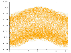
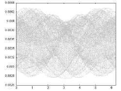
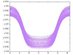
Figure 1. Projections of the 3D invariant torus in Delaunay coordinates onto $(\ell_{1},L_{1})$, $(\ell_{2},L_{2})$ and $(\hat{g},\hat{G})$ components.

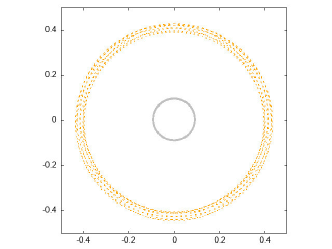
Figure 2. Projections of the 3D invariant torus (generating a 4D torus) in Cartesian coordinates onto positions $x_{1}=(x_{1,1},x_{1,2})$, $x_{2}=(x_{2,1},x_{2,2})$ and momenta $y_{1}=(y_{1,1},y_{1,2})$, $y_{2}=(y_{2,1},y_{2,2})$. Coordinates $x_{1},y_{1}$ correspond to Jupiter and $x_{2},y_{2}$ correspond to Saturn, and are plot in orange and grey, respectively.

From this last torus we have estimated how fast the Fourier coefficients decrease and, so, its analiticity radius. To do so, we have fit the Fourier coefficients of the complexifications $K^{\ell_{1}}+{\mathrm{i}}K^{L_{1}}$, $K^{\ell_{2}}+{\mathrm{i}}K^{L_{2}}$ and $K^{\hat{g}}+{\mathrm{i}}K^{\hat{G}}$ with respect to each of the angles $\theta^{\ell_{1}},\theta^{\ell_{2}},\theta^{\hat{g}}$, thus obtaining estimates of the the analyticity strips $\rho_{\ell_{1}},\rho_{\ell_{2}},\rho_{\hat{g}}$. The results are shown in Figure 3 where, for a Fourier expansion

$$f(\theta^{\ell_{1}},\theta^{\ell_{2}},\theta^{\hat{g}})=\sum_{k_{\ell_{1}},k_{\ell_{2}},k_{\hat{g}}}f_{k_{\ell_{1}},k_{\ell_{2}},k_{\hat{g}}}e^{\mathrm{i}(k_{\ell_{1}}\theta^{\ell_{1}}+k_{\ell_{2}}\theta^{\ell_{2}}+k_{\hat{g}}\theta^{\hat{g}})},$$

we fit the analyticity strips $\rho_{\ell_{1}},\rho_{\ell_{2}},\rho_{\hat{g}}$ of each of the angles by considering the univariate Fourier series

$$\tilde{f}_{\ell_{1}}(\theta^{\ell_{1}})=\sum_{k_{\ell_{1}}}\left(\sum_{k_{\ell_{2}},k_{\hat{g}}}|f_{k_{\ell_{1}},k_{\ell_{2}},k_{\hat{g}}}|\right)e^{\mathrm{i}(k_{\ell_{1}}\theta^{\ell_{1}})},\quad\tilde{f}_{\ell_{2}}(\theta^{\ell_{2}})=\sum_{k_{\ell_{2}}}\left(\sum_{k_{\ell_{1}},k_{\hat{g}}}|f_{k_{\ell_{1}},k_{\ell_{2}},k_{\hat{g}}}|\right)e^{\mathrm{i}(k_{\ell_{2}}\theta^{\ell_{2}})},$$

$$\tilde{f}_{\hat{g}}(\theta^{\hat{g}})=\sum_{k_{\hat{g}}}\left(\sum_{k_{\ell_{1}},k_{\ell_{2}}}|f_{k_{\ell_{1}},k_{\ell_{2}},k_{\hat{g}}}|\right)e^{\mathrm{i}(k_{\hat{g}}\theta^{\hat{g}})}$$

and doing a standard fit on their coefficients.

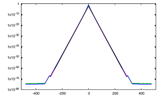
$\theta^{\ell_{1}}$	$\theta^{\ell_{2}}$
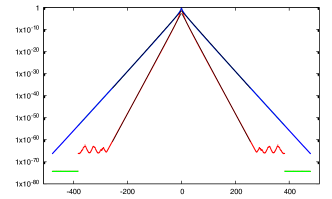
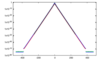
$\theta^{\hat{g}_{1}}$	$K^{\ell_{1}}+{\mathrm{i}}K^{L_{1}}$ $K^{\ell_{2}}+{\mathrm{i}}K^{L_{2}}$ $K^{\hat{g}}+{\mathrm{i}}K^{\hat{G}}$ $\rho_{\ell_{1}}$ 0.524453 0.521794 0.522239 $\rho_{\ell_{2}}$ 0.416514 0.417078 0.417001 $\rho_{\hat{g}}$ 0.525773 0.316526 0.316557

Figure 3. Fits of Fourier coefficients of the (complexified) components of the parameterization $\tilde{f}_{\ell_{1}},\tilde{f}_{\ell_{2}}$ and $\tilde{f}_{\hat{g}}$, and estimates of analyticity strips.

5. Numerical verification of the KAM constants

The numerical certification of the existence of the invariant torus is based on the KAM Theorem and the Iterative Lemma appearing in [20]. For the sake of completeness, we include their tailored and simplified versions (with the most relevant hypotheses) in appendix A, so it will guide us in all the data needed for doing the validation. For the specific expression of all the constants we refer the reader to [20], where they appear in the appendices.

Given the $\omega=(\omega^{\ell},\omega^{\hat{g}_{1}})$ in (4.1), (4.2) we can certify (using the validation techniques in [21]) that at distance $10^{-80}$ there is a Diophantine vector with $\tau=2.4$ and $\gamma=1.69\cdot 10^{-6}$. Moreover, we choose the radius of analiticity to be $\rho=0.1$ and $\delta=\frac{\rho}{6}$.

The hypotheses in $H_{1}$ control the Hamiltonian and its associated vector field in a tubular neighborhood of the torus $K({\mathbb{T}}^{m}_{\rho})$. In our case, it is enough to take these constants to be

$$c_{\text{\tiny${X_{h}}$}}=0.09,c_{\text{\tiny${\rm D}{X_{h}}$}}=129,c_{\text{\tiny$({\rm D}{X_{h}})^{\!\top}$}}=129,c_{\text{\tiny${\rm D}^{2}{X_{h}}$}}=5\cdot 10^{10}.$$

The hypotheses in $H_{2}$ control the parameterization $K$ and all the geometric infomation it has (the bunbles $DK$, $N$ and so on). In our case, these constants are computed with the approximation and obtained

$$\|DK\|=4.7811815833,\|DK^{T}\|=6.8755882886,\|B\|=7.35806411265,$$

$$\|{N}\|=3.5704498717,\|{{N}}^{\!\top}\|=2.8621242724,|\langle{T}\rangle|^{-1}=354.07743243.$$

The corresponding $\sigma$ constants are obtained by multipling these norms by a factor $1+10^{-10}$.

With this information we can run the Iterative Lemma several steps, say 10, and with different initial invariance errors and then apply the KAM Theorem to see if it converges (Inequality (A.1) is fulfilled). We have obtained that with $\|\eta^{{\rm D}\!K}\|=10^{-38},\|\eta^{N}\|=10^{-44}$. However, from our numerics we obtain that our torus satisfies $\|\eta^{{\rm D}\!K}\|=3.6\cdot 10^{-54}$ and $\|\eta^{N}\|=1.7\cdot 10^{-57}$, which are very much smaller than the thresholds!

6. Computation details

For running the continuation method on the translated torus algorithm from the integrable system, we run the programs is an out to date MacBook Air laptop with one CPU 1.7 GHz Dual-Core Intel i7 and RAM memory 8G, since for the approximation we work with long double C arithmetics and the tori are discretized in $128^{3}$ nodes, accounting to 32M of memory for each of the six components of the parameterization of the torus. We have also adapted and tested the programs to work with quadruple precision __float128 C arithmetics. For the invariant torus algorithm, we have used an iMac Pro with one CPU 3,2 GHz Intel Xeon W with 8 cores and RAM Memory 256G, working with several extended precision arithmetics with mpfr (up to 76 decimal digits, that correspond to 64 bytes, respectively) and the torus is discretized in $1024^{3}$ nodes , accounting 64G of memory for each to the components. This last computation has also been run in the UPPMAX supercomputer.

Finally, we give some numbers to provide an idea of the order of magnitude of the managed data structures at the final stages of the computations. The data structures are complex vectors, that store couples of real grids. Moreover, handling of memory (both RAM and disc) by mpfr is anisotropic. For instance, for the computation of the torus with 76 digits the program uses up to 194G of RAM memory for handling one single complex grid of size $1024^{3}$, and 891G of memory disk to store the objects being computed by the program. For files storing the same number of mpfr objects, $2\cdot 1024^{3}/8$, the sizes range from 87M to 8.8G.

7. Acknowledgements

The authors are grateful to Alejandro Luque, Kristian Bjerklöv, Chiara Caracciolo and Andreas Strömbergsson for fruitful discussions.

J.-Ll.F. has been partially supported by the Swedish VR Grant 2019-04591, and A.H. has been supported by the Spanish grant PID2021-125535NB-I00 (MCIU/AEI/FEDER, UE), and by the Spanish State Research Agency, through the Severo Ochoa and María de Maeztu Program for Centers and Units of Excellence in R&D (CEX2020-001084-M). Some computations were enabled by resources in project NAISS 2023/5-192 provided by the National Academic Infrastructure for Supercomputing in Sweden (NAISS) at UPPMAX, funded by the Swedish Research Council through grant agreement no. 2022-06725.

Appendix A KAM Theorem and Iterative Lemma

Here we gather both the KAM Theorem and the Iterative Lemma in a tailored form. For a more detailed exposition of them have a look at [20].

Theorem A.1.

Let $h:{\mathcal{U}}\rightarrow{\mathbb{C}}$ be a real-analytic Hamiltonian, defined in an open set ${\mathcal{U}}\subset{\mathbb{T}}_{\mathbb{C}}^{m}\times{\mathbb{C}}^{m}$. Let $K:\bar{\mathbb{T}}^{m}_{\rho}\rightarrow{\mathcal{U}}$ be a continuous map, real-analytic in ${\mathbb{T}}^{m}_{\rho}$, whose derivatives are also continuous in $\bar{\mathbb{T}}^{m}_{\rho}$, defining an homotopic to the zero-section embedding of $\bar{\mathbb{T}}^{m}_{\rho}$ into ${\mathbb{T}}_{\mathbb{C}}^{m}\times{\mathbb{C}}^{m}$ (in particular $K(\theta)-(\theta,0)$ is $2\pi$-periodic). Let $\omega\in{\mathcal{D}}_{\gamma,\tau}^{m}$ be a Diophantine vector, for some $\gamma>0$ and $\tau\geq m-1$. We also assume:

• There exist constants $c_{\text{\tiny${X_{h}}$}}$, $c_{\text{\tiny${\rm D}{X_{h}}$}}$, $c_{\text{\tiny$({\rm D}{X_{h}})^{\!\top}$}}$, $c_{\text{\tiny${\rm D}^{2}{X_{h}}$}}$ such that

  $$\left\|{{X_{h}}}\right\|_{{\mathcal{U}}}\leq c_{\text{\tiny${X_{h}}$}},\quad\left\|{{\mbox{\rm D}}{X_{h}}}\right\|_{{\mathcal{U}}}\leq c_{\text{\tiny${\rm D}{X_{h}}$}},\quad\left\|{({\mbox{\rm D}}{X_{h}})^{\!\top}}\right\|_{{\mathcal{U}}}\leq c_{\text{\tiny$({\rm D}{X_{h}})^{\!\top}$}},\quad\left\|{{\mbox{\rm D}}^{2}{X_{h}}}\right\|_{{\mathcal{U}}}\leq c_{\text{\tiny${\rm D}^{2}{X_{h}}$}}.$$

• There are condition numbers $\sigma_{\mbox{{\tiny${\rm D}K$}}}$, $\sigma_{\mbox{{\tiny$({\rm D}K)\!^{\!\top}$}}}$, $\sigma_{B}$, $\sigma_{\mbox{{\tiny${N}$}}}$, $\sigma_{\mbox{{\tiny${{N}}^{\!\top}$}}}$, and $\sigma_{\mbox{{\tiny{$\langle{T}\rangle^{\mbox{-}1}$}}}}$ such that

  $$\left\|{{{\mbox{\rm D}}{K}}}\right\|_{\rho}<\sigma_{\mbox{{\tiny${\rm D}K$}}},\quad\left\|{({{\mbox{\rm D}}{K}})^{{\!\top}}}\right\|_{\rho}<\sigma_{\mbox{{\tiny$({\rm D}K)\!^{\!\top}$}}},\quad\left\|{{B}}\right\|_{\rho}<\sigma_{B},$$

  $$\left\|{{N}}\right\|_{\rho}<\sigma_{\mbox{{\tiny${N}$}}},\quad\left\|{{{N}}^{\!\top}}\right\|_{\rho}<\sigma_{\mbox{{\tiny${{N}}^{\!\top}$}}},\quad|{\langle{T}\rangle^{\text{-}1}}|<\sigma_{\mbox{{\tiny{$\langle{T}\rangle^{\mbox{-}1}$}}}};$$

Then, for each $\delta\in]0,\rho/6[$, there exists constants $\mathfrak{C},\mathfrak{C}_{\Delta K}$ depending on $\rho,\delta$ and the above constants and objects, such that, if

(A.1) $$\frac{\mathfrak{C}}{\gamma\delta^{\tau+1}}{{\ \max\left\{\left\|{\eta^{{\rm D}\!K}}\right\|_{\rho},\frac{1}{\gamma\delta^{\tau}}\left\|{\eta^{N}}\right\|_{\rho}\right\}}}<1,$$

where $\eta^{{\rm D}\!K}=-{{N}}^{\!\top}\Omega\>({\mathfrak{L}_{\omega}}{K}+{X_{h}}{\!\>\circ\!\,}K),\ \eta^{N}={({{\mbox{\rm D}}{K}})^{{\!\top}}}\Omega\>({\mathfrak{L}_{\omega}}{K}+{X_{h}}{\!\>\circ\!\,}K),$ then, for $\rho_{\infty}=\rho-6\delta$, there exists $K_{\infty}:\bar{\mathbb{T}}^{m}_{\rho_{\infty}}\rightarrow{\mathcal{U}}$ continuous, real-analytic in ${\mathbb{T}}^{m}_{\rho_{\infty}}$, whose derivatives are also continuous in $\bar{\mathbb{T}}^{m}_{\rho_{\infty}}$, defining an homotopic to the zero-section embedding of $\bar{\mathbb{T}}^{m}_{\rho_{\infty}}$ into ${\mathcal{U}}$ that is invariant under ${X_{h}}$, with frequency $\omega$, so that

$${\mathfrak{L}_{\omega}}{K}_{\infty}+{X_{h}}{\!\>\circ\!\,}{K}_{\infty}=0.$$

Moreover, ${K}_{\infty}$ satisfies hypothesis $H_{2}$, in ${\mathbb{T}}^{m}_{\rho_{\infty}}$, and it is close to $K$:

$$\left\|{{K}_{\infty}-{K}}\right\|_{\rho_{\infty}}\leq\frac{\mathfrak{C}_{\Delta K}}{\gamma\delta^{\tau}}{{\ \max\left\{\left\|{\eta^{{\rm D}\!K}}\right\|_{\rho},\frac{1}{\gamma\delta^{\tau}}\left\|{\eta^{N}}\right\|_{\rho}\right\}}}.$$

The proof of the previous theorem consists of iteratively applying the following lemma.

Lemma A.2 (The Iterative Lemma).

Let us be under the same hypotheses as in Theorem A.1. For any $\delta\in]0,\rho/3]$, there exist constants $C_{\mathrm{sym}}$, $C_{\xi^{\text{\tiny$L$}}}$, $C_{\Delta{\bar{\bar{K}}}}$, $C_{\Delta{\rm D}{\bar{\bar{K}}}}$, $C_{\Delta({\rm D}{\bar{\bar{K}}})^{\!\top}}$, $C_{\Delta{\bar{\bar{B}}}}$, $C_{\Delta{\bar{\bar{{N}}}}}$, $C_{\Delta{\bar{\bar{N}}}\phantom{)}\!\!^{{\!\top}}}$, $C_{\Delta\langle{{\bar{\bar{T}}}}\rangle^{\text{-}1}}$, $\hat{C}_{\Delta}$ and $Q_{{{{\bar{\bar{\eta}}}}^{L}}}$, $Q_{{{\bar{\bar{\eta}}}^{N}}}$, such that if

$$\frac{\hat{C}_{\Delta}}{\gamma\delta^{\tau+1}}{{\ \max\left\{\left\|{\eta^{{\rm D}\!K}}\right\|_{\rho},\frac{1}{\gamma\delta^{\tau}}\left\|{\eta^{N}}\right\|_{\rho}\right\}}}<1,$$

then we have a new real-analytic parameterization ${\bar{\bar{K}}}:\bar{\mathbb{T}}^{m}_{\rho-2\delta}\rightarrow{\mathcal{U}}$, that defines new objects ${{\mbox{\rm D}}{\bar{\bar{K}}}}$, ${\bar{\bar{B}}}$, ${\bar{\bar{{N}}}}$ and ${\bar{\bar{T}}}$ (obtained replacing ${K}$ by ${\bar{\bar{K}}}$ in the corresponding definitions) satisfying

$$\left\|{{{\mbox{\rm D}}{\bar{\bar{K}}}}}\right\|_{\rho-3\delta}<\sigma_{\mbox{{\tiny${\rm D}K$}}},\left\|{({{\mbox{\rm D}}{\bar{\bar{K}}}})^{{\!\top}}}\right\|_{\rho-3\delta}<\sigma_{\mbox{{\tiny$({\rm D}K)\!^{\!\top}$}}},\left\|{{\bar{\bar{B}}}}\right\|_{\rho-3\delta}<\sigma_{B},$$

$$\left\|{{\bar{\bar{{N}}}}}\right\|_{\rho-3\delta}<\sigma_{\mbox{{\tiny${N}$}}},\left\|{{\bar{\bar{N}}}\phantom{)}\!\!^{{\!\top}}}\right\|_{\rho-3\delta}<\sigma_{\mbox{{\tiny${{N}}^{\!\top}$}}},|{\langle{{\bar{\bar{T}}}}\rangle^{\text{-}1}}|<\sigma_{\mbox{{\tiny{$\langle{T}\rangle^{\mbox{-}1}$}}}},$$

and

$$\left\|{{\bar{\bar{K}}}-{K}}\right\|_{\rho-2\delta}\leq\frac{C_{\Delta{\bar{\bar{K}}}}}{\gamma\delta^{\tau}}{{\ \max\left\{\left\|{\eta^{{\rm D}\!K}}\right\|_{\rho},\frac{1}{\gamma\delta^{\tau}}\left\|{\eta^{N}}\right\|_{\rho}\right\}}},$$

$$\left\|{{{\mbox{\rm D}}{\bar{\bar{K}}}}-{{\mbox{\rm D}}{K}}}\right\|_{\rho-3\delta}\leq\frac{C_{\Delta{\rm D}{\bar{\bar{K}}}}}{\gamma\delta^{\tau+1}}{{\ \max\left\{\left\|{\eta^{{\rm D}\!K}}\right\|_{\rho},\frac{1}{\gamma\delta^{\tau}}\left\|{\eta^{N}}\right\|_{\rho}\right\}}},$$

$$\left\|{({{\mbox{\rm D}}{\bar{\bar{K}}}})^{{\!\top}}-({{\mbox{\rm D}}{K}})^{{\!\top}}}\right\|_{\rho-3\delta}\leq\frac{C_{\Delta({\rm D}{\bar{\bar{K}}})^{\!\top}}}{\gamma\delta^{\tau+1}}{{\ \max\left\{\left\|{\eta^{{\rm D}\!K}}\right\|_{\rho},\frac{1}{\gamma\delta^{\tau}}\left\|{\eta^{N}}\right\|_{\rho}\right\}}},$$

$$\left\|{{\bar{\bar{B}}}-{B}}\right\|_{\rho-3\delta}\leq\frac{C_{\Delta{\bar{\bar{B}}}}}{\gamma\delta^{\tau+1}}{{\ \max\left\{\left\|{\eta^{{\rm D}\!K}}\right\|_{\rho},\frac{1}{\gamma\delta^{\tau}}\left\|{\eta^{N}}\right\|_{\rho}\right\}}},$$

$$\left\|{{\bar{\bar{{N}}}}-{N}}\right\|_{\rho-3\delta}\leq\frac{C_{\Delta{\bar{\bar{{N}}}}}}{\gamma\delta^{\tau+1}}{{\ \max\left\{\left\|{\eta^{{\rm D}\!K}}\right\|_{\rho},\frac{1}{\gamma\delta^{\tau}}\left\|{\eta^{N}}\right\|_{\rho}\right\}}},$$

$$\left\|{{\bar{\bar{N}}}\phantom{)}\!\!^{{\!\top}}-{{N}}^{\!\top}}\right\|_{\rho-3\delta}\leq\frac{C_{\Delta{\bar{\bar{N}}}\phantom{)}\!\!^{{\!\top}}}}{\gamma\delta^{\tau+1}}{{\ \max\left\{\left\|{\eta^{{\rm D}\!K}}\right\|_{\rho},\frac{1}{\gamma\delta^{\tau}}\left\|{\eta^{N}}\right\|_{\rho}\right\}}},$$

$$|{\langle{{\bar{\bar{T}}}}\rangle^{\text{-}1}-\langle{{T}}\rangle^{\text{-}1}}|\leq\frac{C_{\Delta\langle{{\bar{\bar{T}}}}\rangle^{\text{-}1}}}{\gamma\delta^{\tau+1}}{{\ \max\left\{\left\|{\eta^{{\rm D}\!K}}\right\|_{\rho},\frac{1}{\gamma\delta^{\tau}}\left\|{\eta^{N}}\right\|_{\rho}\right\}}}.$$

Moreover, the tangent and normal components of the new error of invariance

$${\bar{\bar{E}}}={X_{h}}{\!\>\circ\!\,}{\bar{\bar{K}}}+{\mathfrak{L}_{\omega}}{\bar{\bar{K}}},$$

satisfy

$$\left\|{{{\bar{\bar{\eta}}}^{N}}}\right\|_{\rho-3\delta}\leq\frac{Q_{{{\bar{\bar{\eta}}}^{N}}}}{\delta}{{{{\ \max\left\{\left\|{\eta^{{\rm D}\!K}}\right\|_{\rho},\frac{1}{\gamma\delta^{\tau}}\left\|{\eta^{N}}\right\|_{\rho}\right\}}}}^{2}},$$

and

$$\begin{split}\left\|{{{{\bar{\bar{\eta}}}}^{L}}}\right\|_{\rho-3\delta}&\leq\frac{Q_{{{{\bar{\bar{\eta}}}}^{L}}}}{\gamma\delta^{\tau+1}}{{{{\ \max\left\{\left\|{\eta^{{\rm D}\!K}}\right\|_{\rho},\frac{1}{\gamma\delta^{\tau}}\left\|{\eta^{N}}\right\|_{\rho}\right\}}}}^{2}}.\end{split}$$

References

• [1] Planetary fact sheet - metric. https://nssdc.gsfc.nasa.gov/planetary/factsheet/. Accessed: 2023-12-05.
• [2] Sun fact sheet. https://nssdc.gsfc.nasa.gov/planetary/factsheet/sunfact.html. Accessed: 2023-12-05.
• [3] V. I. Arnold. On the classical perturbation theory and the stability problem of planetary systems. Dokl. Akad. Nauk SSSR, 145:487–490, 1962.
• [4] V.I. Arnold. Proof of a theorem of A. N. Kolmogorov on the preservation of conditionally periodic motions under a small perturbation of the Hamiltonian. Uspehi Mat. Nauk, 18(5 (113)):13–40, 1963.
• [5] V.I. Arnold. Small denominators and problems of stability of motion in classical and celestial mechanics. Russ. Math. Surveys, 18:85–192, 1963.
• [6] H.W. Broer, G.B. Huitema, and M.B. Sevryuk. Quasi-periodic motions in families of dynamical systems. Order amidst chaos. Lecture Notes in Math., Vol 1645. Springer-Verlag, Berlin, 1996.
• [7] R. Calleja, A. Celletti, and R. de la Llave. A KAM theory for conformally symplectic systems: efficient algorithms and their validation. J. Differential Equations, 255(5):978–1049, 2013.
• [8] T. Castan, J. Féjoz, A. Chenciner, L.N. ), A.I. Neishtadt, L.C. ), J.P.M. ), V.Y. Kaloshin, E. Séré, Hauts-de-Seine / 1992-….). École doctorale Astronomie et astrophysique d’Île-de France (Meudon, et al. Stability in the Plane Planetary Three-body Problem. 2017.
• [9] A. Celletti and L. Chierchia. A constructive theory of Lagrangian tori and computer-assisted applications. In Dynamics Reported, pages 60–129. Springer, Berlin, 1995.
• [10] R. Chandra, L. Dagum, D. Kohr, R. Menon, D. Maydan, and J. McDonald. Parallel programming in OpenMP. Morgan kaufmann, 2001.
• [11] L. Chierchia. KAM lectures. In Dynamical systems. Part I, Pubbl. Cent. Ric. Mat. Ennio Giorgi, pages 1–55. Scuola Norm. Sup., Pisa, 2003.
• [12] L. Chierchia and G. Pinzari. The planetary $N$-body problem: symplectic foliation, reductions and invariant tori. Invent. Math., 186(1):1–77, 2011.
• [13] S. Das, Y. Saiki, E. Sander, and J. A. Yorke. Quantitative quasiperiodicity. Nonlinearity, 30(11):4111–4140, 2017.
• [14] R. de la Llave. A tutorial on KAM theory. In Smooth ergodic theory and its applications (Seattle, WA, 1999), volume 69 of Proc. Sympos. Pure Math., pages 175–292. Amer. Math. Soc., Providence, RI, 2001.
• [15] R. de la Llave, A. González, À. Jorba, and J. Villanueva. KAM theory without action-angle variables. Nonlinearity, 18(2):855–895, 2005.
• [16] H.S. Dumas. The KAM story. World Scientific Publishing Co. Pte. Ltd., Hackensack, NJ, 2014. A friendly introduction to the content, history, and significance of classical Kolmogorov-Arnold-Moser theory.
• [17] J. Féjoz. Démonstration du ‘théorème d’Arnold’ sur la stabilité du système planétaire (d’après Herman). Ergodic Theory Dynam. Systems, 24(5):1521–1582, 2004.
• [18] Jacques Féjoz. Introduction to KAM theory with a view to celestial mechanics. In Variational methods, volume 18 of Radon Ser. Comput. Appl. Math., pages 387–433. De Gruyter, Berlin, 2017.
• [19] J.-Ll Figueras and A. Haro. A Computer-Assisted Proof of the Existence of Quasiperiodic Solutions of the planar Sun-Jupiter-Saturn Problem with Realistic Data. (In progress).
• [20] J.-Ll Figueras and A. Haro. A modified parameterization method for invariant Lagrangian tori for partially integrable Hamiltonian systems. (Accepted in Physica D).
• [21] J.-Ll. Figueras, A. Haro, and A. Luque. Rigorous Computer-Assisted Application of KAM Theory: A Modern Approach. Found. Comput. Math., 17(5):1123–1193, 2017.
• [22] J.-Ll. Figueras, A. Haro, and A. Luque. Effective bounds for the measure of rotations. Nonlinearity, 33(2):700–741, 2020.
• [23] L. Fousse, G. Hanrot, V. Lefèvre, P. Pélissier, and P. Zimmermann. Mpfr: A multiple-precision binary floating-point library with correct rounding. ACM Trans. Math. Softw., 33(2):13–es, jun 2007.
• [24] G. Gómez, J.-M. Mondelo, and C. Simó. A collocation method for the numerical Fourier analysis of quasi-periodic functions. I. Numerical tests and examples. Discrete Contin. Dyn. Syst. Ser. B, 14(1):41–74, 2010.
• [25] A. González, A. Haro, and R. de la Llave. Singularity theory for non-twist KAM tori. Mem. Amer. Math. Soc., 227(1067):vi+115, 2014.
• [26] A. González, À. Haro, and R. de la Llave. Efficient and reliable algorithms for the computation of non-twist invariant circles. Found. Comput. Math., 22(3):791–847, 2022.
• [27] A. Haro, M. Canadell, J.-Ll. Figueras, A. Luque, and J.-M. Mondelo. The parameterization method for invariant manifolds, volume 195 of Applied Mathematical Sciences. Springer, [Cham], 2016. From rigorous results to effective computations.
• [28] A. Haro and A. Luque. A-posteriori KAM theory with optimal estimates for partially integrable systems. J. Differential Equations, 266(2-3):1605–1674, 2019.
• [29] M. Hénon. Exploration numérique du problème restreint iv. masses égales, orbites non périodiques. Bull. Astronom., 3(1–2):49–66, 1966.
• [30] M.-R. Herman. Démonstration d’un théorème de V.I. Arnold. Séminaire de Syst‘emes Dynamiques et manuscript, 1998.
• [31] A.N. Kolmogorov. On conservation of conditionally periodic motions for a small change in Hamilton’s function. Dokl. Akad. Nauk SSSR (N.S.), 98:527–530, 1954. Translated in p. 51–56 of Stochastic Behavior in Classical and Quantum Hamiltonian Systems, Como 1977 (eds. G. Casati and J. Ford) Lect. Notes Phys. 93, Springer, Berlin, 1979.
• [32] J. Laskar. Frequency map analysis and quasiperiodic decompositions. In Hamiltonian systems and Fourier analysis, Adv. Astron. Astrophys., pages 99–133. Camb. Sci. Publ., Cambridge, 2005.
• [33] J. Laskar. Michel hénon and the stability of the solar system. In Hermann, editor, Une vie dédiée aux systèmes dynamiques: Hommage a Michel Hénon, pages 71–79. 2016.
• [34] J. Laskar and P. Robutel. Stability of the planetary three-body problem. I. Expansion of the planetary Hamiltonian. Celestial Mech. Dynam. Astronom., 62(3):193–217, 1995.
• [35] U. Locatelli and A. Giorgilli. Construction of Kolmogorov’s normal form for a planetary system. Regul. Chaotic Dyn., 10(2):153–171, 2005.
• [36] U. Locatelli and A. Giorgilli. Invariant tori in the Sun-Jupiter-Saturn system. Discrete Contin. Dyn. Syst. Ser. B, 7(2):377–398 (electronic), 2007.
• [37] A. Luque and J. Villanueva. Numerical computation of rotation numbers for quasi-periodic planar curves. Phys. D, 238(20):2025–2044, 2009.
• [38] J. Moser. On invariant curves of area-preserving mappings of an annulus. Nachr. Akad. Wiss. Göttingen Math.-Phys. Kl. II, 1962:1–20, 1962.
• [39] J. Moser. Convergent series expansions for quasi-periodic motions. Math. Ann., 169:136–176, 1967.
• [40] I. S. Newton. Philosophiae naturalis principia mathematica. William Dawson & Sons, Ltd., London, 1687.
• [41] H. Poincaré. The three-body problem and the equations of dynamics, volume 443 of Astrophysics and Space Science Library. Springer, Cham, 2017. Poincaré’s foundational work on dynamical systems theory, Translated from the 1890 French original and with a preface by Bruce D. Popp.
• [42] W.H. Press, S.A. Teukolsky, W.T. Vetterling, and B.P. Flannery. Numerical Recipes in C: The Art of Scientific Computing. Cambridge University Press, second edition edition, 2002.
• [43] P. Robutel. Stability of the planetary three-body problem. II. KAM theory and existence of quasiperiodic motions. Celestial Mech. Dynam. Astronom., 62(3):219–261, 1995.
• [44] J. Villanueva. A new approach to the parameterization method for Lagrangian tori of Hamiltonian systems. J. Nonlinear Sci., 27(2):495–530, 2017.