NLP Verification: Towards a General Methodology for Certifying Robustness

Abstract

Deep neural networks (DNNs) have exhibited substantial success in the field of Natural Language Processing (NLP). As these systems are increasingly integrated into real-world applications, ensuring their safety and reliability becomes a primary concern. There are safety critical contexts where such models must be robust to variability or attack, and give guarantees over their output. Computer Vision had pioneered the use of formal verification for neural networks for such scenarios and developed common verification standards and pipelines. In contrast, NLP verification methods have only recently appeared in the literature. While presenting sophisticated algorithms on their own right, these papers have not yet crystallised into a common methodology, they are often light on the pragmatical issues of NLP verification, and the area remains fragmented.

In this paper, we make an attempt to distil and evaluate general components of an NLP verification pipeline, that emerges from the progress in the field to date. Our contributions are two-fold.

Firstly, we give a general (i.e. algorithm-independent) characterisation of verifiable subspaces that result from embedding sentences into continuous spaces. We identify, and give an effective method to deal with, the technical challenge of semantic generalisability of verified subspaces; and propose it as a standard metric in the NLP verification pipelines (alongside with the standard metrics of model accuracy and model verifiability).

Secondly, we propose a general methodology to analyse the effect of the embedding gap – a problem that refers to the discrepancy between verification of geometric subpspaces on the one hand, and semantic meaning of sentences which the geometric subspaces are supposed to represent, on the other hand. In extreme cases, poor choices in embedding of sentences may invalidate verification results. We propose a number of practical NLP methods that can help to identify the effects of the embedding gap; and in particular we propose the metric of falsifiability of semantic subpspaces that we propose as another fundamental metric to be reported as part of the NLP verification pipeline.

We believe that together these general principles pave the way towards a more consolidated and effective development of this new domain.

0.1 Introduction

Deep neural networks (DNNs) have demonstrated remarkable success at addressing challenging problems in various areas, such as Computer Vision (CV) [102] and Natural Language Processing (NLP) [113, 49]. However, as DNN-based systems are increasingly deployed in safety-critical applications [10, 125, 11, 34, 13, 35], ensuring their safety and security becomes paramount. Current NLP systems cannot guarantee either truthfulness, accuracy, faithfulness, or groundedness of outputs given an input query, which can lead to different levels of harm.

Contexts which necessitate guaranteed outputs.

One such example in the NLP domain is the requirement of a chatbot to correctly disclose non-human identity, when prompted by the user to do so. Recently there have been several pieces of legislation proposed that will enshrine this requirement in law [63, 68]. In order to be compliant with these new laws, in theory the underlying DNN of the chatbot (or the sub-system responsible for identifying these queries) must be 100% accurate in its recognition of such a query. However, a central theme of generative linguistics going back to von Humboldt, is that language is ‘an infinite use of finite means’, i.e there exists many ways to say the same thing. In reality the questions can come in a near infinite number of different forms, all with similar semantic meanings. For example: “Are you a Robot?”, “Am I speaking with a person?”, “Am i texting to a real human?”, “Aren’t you a chatbot?”. Failure to recognise the user’s intent and thus failure to answer the question correctly could potentially have legal implications for designers of these systems [63, 68].

Similarly, as such systems become widespread in their use, it may be desirable to have guarantees on queries concerning safety critical domains, for example when the user asks for medical advice. Research has shown that users tend to attribute undue expertise to systems [2, 34] potentially causing real world harm [12] (e.g. ‘Is it safe to take these painkillers with a glass of wine?’). However, a question remains on how to ensure that NLP systems can give formally guaranteed outputs, particularly for scenarios that require maximum control over the output.

Formal verification of neural networks.

One possible solution has been to apply formal verification techniques to deep neural networks (DNN), which aims at ensuring that for every possible input, the output generated by the network satisfies the desired properties— such as guaranteeing that a system will accurately disclose its non-human identity. Generally, in DNN robustness verification, the aim is to guarantee that every point in a given region of the embedding space is classified correctly. Concretely, given a DNN $N:^{m}\rightarrow^{n}$, one formulates an effective algorithm to define subspaces $\mathcal{S}_{1},\ldots,\mathcal{S}_{l}$ of the vector space ^m. For example, one can define “$\epsilon\text{-cubes}$" or “$\epsilon\text{-balls}$" around all input vectors given by the data set in question (in which case the number of $\mathcal{S}_{1},\ldots,\mathcal{S}_{l}$ will correspond to the number of samples in the given data set). Then, using a separate verification algorithm $\mathcal{V}$, we verify whether $N$ is robust for each $\mathcal{S}_{i}$, i.e. whether $N$ assigns the same class for all vectors contained in $\mathcal{S}_{i}$. Note that each $\mathcal{S}_{i}$ is itself infinite (i.e. continuous), and thus $\mathcal{V}$ is usually based on equational reasoning, abstract interpretation or bound propagation, see the related work section. All $\mathcal{S}_{i}$ for which $N$ is proven robust, form verified subspaces of the given vector space (for $N$). The percentage of verified subspaces (among $\mathcal{S}_{1},\ldots,\mathcal{S}_{l}$) is called verification success rate (or verifiability). Given $\mathcal{S}_{1},\ldots,\mathcal{S}_{l}$, we say a DNN $N_{1}$ is more verifiable than $N_{2}$ if $N_{1}$ has higher verification success rate on $\mathcal{S}_{1},\ldots,\mathcal{S}_{l}$. Despite not providing a formal guarantee about the entire embedding space, this result is useful as it provides guarantees about the behaviour of the network over a large set of unseen inputs.

Challenges of NLP verification.

However, existing verification approaches primarily focus on computer vision (CV) tasks, where images are seen as vectors in a continuous space and every point in the space corresponds to a valid image. In contrast, sentences in NLP form a discrete domain, making it challenging to apply traditional verification techniques effectively. In particular, taking an NLP dataset $\mathcal{Y}$ to be a set of sentences $s_{1},\ldots,s_{q}$ written in natural language, an embedding $\mathbb{E}$ is a function that maps a sentence to a vector in ^m. The resulting vector space is called the embedding space. Due to discrete nature of the set $\mathcal{Y}$, the reverse of the embedding function $\mathbb{E}^{-1}:^{m}\rightarrow\mathcal{Y}$ is not total or undefined. This problem is known as the “problem of the embedding gap". Sometimes, one uses the term to more generally refer to any discrepancies that $\mathbb{E}$ introduces, for example, when it maps dissimilar sentences close in ^m. We use the term in both mathematical and NLP sense.

Mathematically, the general (geometric) “DNN robustness verification" approach of defining and verifying subspaces of ^m should work, and some prior works exploit this fact. However, pragmatically, because of the embedding gap only a tiny fraction of vectors contained in the verified subspaces maps back to valid sentences. When a verified subspace contains no or very few sentence embeddings, we say that verified subspace has low generalisability. Low generalisability may render verification efforts obsolete for practical applications.

From the NLP perspective, there are other, more subtle, examples when the embedding gap can manifest. Suppose we succeeded in verifying a DNN robust on some subspace of ^m. Consider an example when the subspace contains sentences that are semantically similar to the sentence: i really like too chat to a human. are you one?. Verification gives us guarantees that the DNN will always identify these sentences as questions about human/robot identity. But suppose the embedding function $\mathbb{E}$ wrongly embedded sentences belonging to an opposite class into this subspace. For example, an LLM Vicuna generates the following sentence as a rephrase of the previous one: Do you take pleasure in having a conversation with someone?. Suppose our verified subspace contained an embedding of this sentence, too, and thus our verified DNN identifies this second sentence to belong to the the same class as the first one. However, the second sentence is not a question about human/robot identity of the agent! When we can find such an example, we say that it falsifies the verification guarantee for the subspace it is contained in. Alternatively, we say that the subpspace is falsifiable.

Contributions

Our main aim is to provide a general and principled verification methodology that bridges the embedding gap when possible; and gives precise metrics to evaluate and report its effects in any case. The contributions split into two main groups, depending whether the embedding gap is approached from mathematical or NLP perspective.

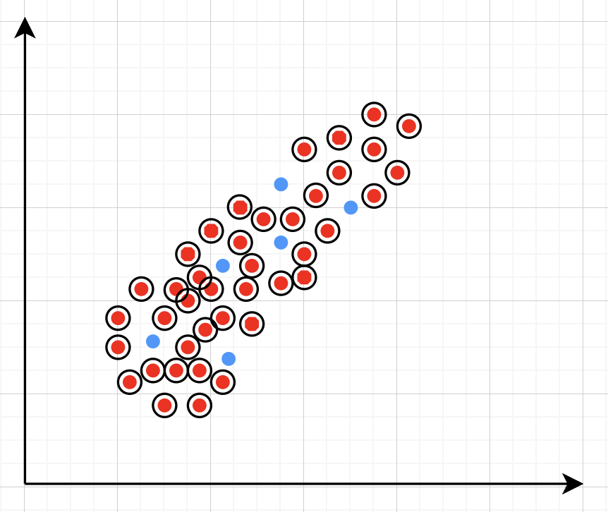
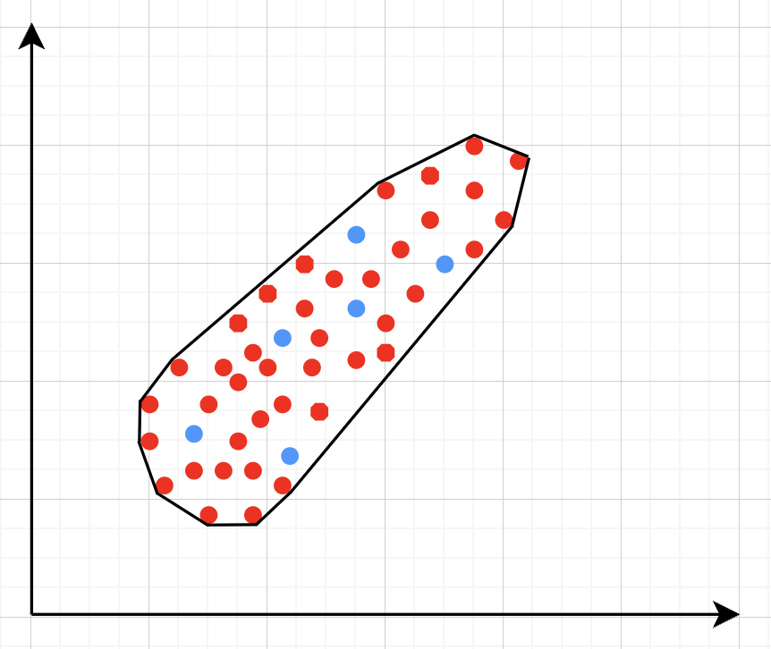
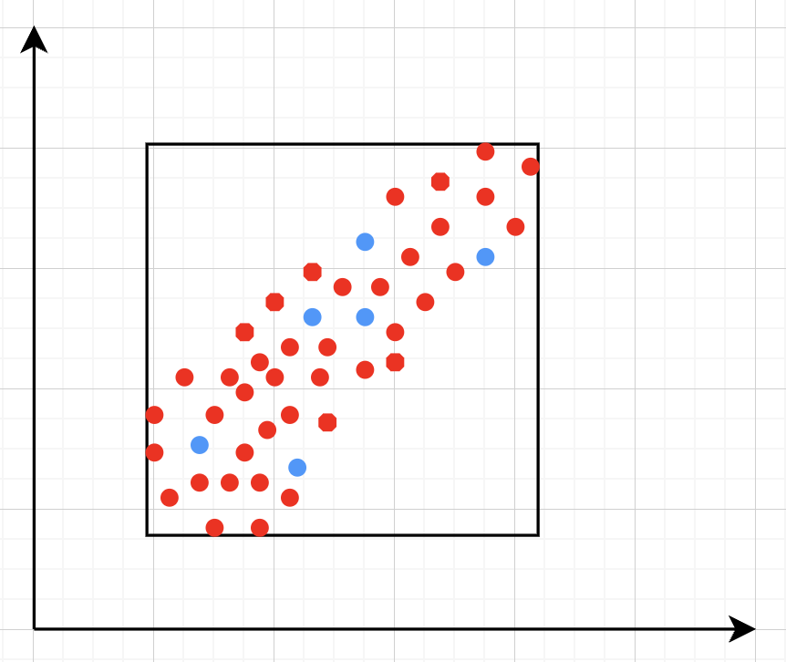
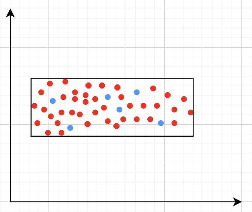
Figure 1: An example of verifiable but not generalisable $\epsilon\text{-balls}$ (left), convex-hull around selected embedded points (centre-left), hyper-rectangle around same points (centre-right) and rotation of such hyper-rectangle (right) in 2-dimensions. The red dots represent sentences in the embedding space from the training set belonging to one class, while the turquoise dots are embedded sentences from the test set belonging to the same class.

Contributions Part 1: Characterisation of verifiable subspaces and NLP verification pipeline.

We start by showing, through a series of experiments, that purely geometric approaches to NLP verification (such as those based on the $\epsilon\text{-ball}$ [107]) suffer from the verifiability-generalisability trade-off: that is, when one metric improves, the other deteriorates. Figure 1 gives a good idea of the problem: the smaller the $\epsilon\text{-ball}$s are, the more verifiable they are, and less generalisable. To the best of our knowledge, this phenomenon has not been reported in the literature before (in the NLP context). We propose a general method for measuring generalisability of the verified subspaces, based on algorithmic generation of semantic attacks on sentences included in the given verified semantic subspace.

An alternative method to purely geometric approach that suffers from the embedding gap is to construct subspaces of the embedding space based on the semantic perturbations of sentences [54, 50, 146]. Concretely, the idea is to form each $\mathcal{S}_{i}$ by embedding a sentence $i$ and its $n$ semantic perturbations into the real vector space and enclosing them inside some geometric shape. Ideally, such a shape should be given by a convex hull around these $n+1$ embedded sentences, however calculating convex hulls with sufficient precision is computationally infeasible for high number of dimensions. Thus, simpler shapes, such as hyper-cubes and hyper-rectangles are used in the literature. We propose a novel refinement of these ideas, by including the method of a hyper-rectangle rotation in order to increase the shape precision (see Figure 1). We will call the resulting shapes semantic subspaces (in contrast to those obtained purely geometrically).

A few questions have been left un-answered in the previous work. Firstly, because generalisability of the verified subspaces is not reported in the literature, we cannot know whether the prior semantically-informed approaches are better in that respect than purely geometric methods. If they are better in both verifiability and generalisability, it is unclear whether the improvement should be attributed to:

• the fact that verified semantic subspaces simply have an optimal volume (for the verifiability-generalisability trade-off), or

• the improved precision of verified subspaces that comes from using the semantic knowledge.

This paper provides a strong argument for including generalisability as a standard metric in reporting NLP verification results in the future. Through a series of experiments, we confirm that verified semantic subspaces are more verifiable and more generalisable than their geometric counterparts. Moreover, by comparing the volumes of the obtained verified semantic and geometric subspaces, we show that the improvement is partly due to finding an optimal size of subspaces (for the given embedding space), and partly due to improvement in shape precision.

The second group of unresolved questions concerns robust training regimes in NLP verification that is used as means of improving verifiability of subspaces in prior works [54, 50, 146]. It was not clear what made robust training successful:

• was it because additional examples generally improved the precision of the decision boundary? (in which case data set augmentation would have a similar effect);

• was it because adversarial examples specifically improved adversarial robustness (in which case simple $\epsilon\text{-ball}$ PGD attacks would have a similar effect); or

• did the knowledge of semantic subspaces play the key role?

Through a series of experiments we show that the latter is the case. In order to do this, we formulate a semantically robust training method that uses projected gradient descent on semantic subspaces (rather than on $\epsilon\text{-balls}$ as the famous PGD algorithm does [85]). We use different forms of semantic perturbations, at character, word and sentence levels (alongside the standard PGD training and data augmentation) to perform semantically robust training. We conclude that semantically robust training generally wins over the standard robust training methods. Moreover, the more sophisticated semantic perturbations we use in semantically robust training, the more verifiable the neural network will be obtained as a result (at no cost to generalisability). For example, using the strongest form of attack (the polyjuice attack [132]) in semantically robust training, we obtain DNNs that are more verifiable irrespective of the way the verified sub-spaces are formed.

As a result, we arrive at a fully parametric approach to NLP verification that disentangles the four components:

• choice of the semantic attack (on the NLP side),

• semantic subspace formation in the embedding space (on the geometric side),

• semantically robust training (on the machine learning side),

• choice of the verification algorithm (on the verification side).

We argue that, together with the new generalisability metric, this approach opens the way for more principled evaluation of performance of NLP verification methods that accounts for the effects of the embedding gap; and generation of more transparent NLP verification benchmarks. We implement a tool that generates NLP verification benchmarks based on the above choices. This paper is the first to use a complete SMT-based verifier (namely Marabou [131]) for NLP verification.

Contributions Part 2: NLP Verification pipeline in use: an NLP perspective on the embedding gap.

We test the theoretical results by suggesting an NLP verification pipeline, a general methodology that starts with NLP analysis of the dataset and obtaining semantically similar perturbations that together characterise the semantic meaning of a sentence; proceeds with embedding of the sentences into the real vector space and defining semantic subspaces around embeddings of semantically similar sentences; and culminates with using these subspaces for both training and verification. This clear division into stages allows us to formulate practical NLP methods for minimising the effects of the embedding gap. In particular, we show that the quality of the generated sentence perturbations maybe improved through the use of human evaluation, cosine similarity and ROUGE-N. We introduce the falsifiability metric as an effective practical way to measure the quality of the embedding functions. Through a detailed case study, we show how geometric and NLP intuitions can be put together at work towards obtaining DNNs that are more verifiable over better generalisable and less falsifiable semantic subspaces. Perhaps more importantly, the proposed methodology opens the way for transparency in reporting NLP verification results, – something that this domain will benefit from if it reaches the stage of practical deplyoment of NLP verification pipelines.

Paper Outline.

From here, the paper proceeds as follows. Section 0.2 gives an extensive literature review encompassing DNN verification methods generally, and NLP verification methods in particular. The section culminates with distilling a common “NLP verification pipeline" encompassing the existing literature. Based on the understanding of major components of the pipeline, the rest of the paper focuses on improving understanding or implementation of its components. Section 0.3 formally defines the components of the pipeline in a general mathematical notation, which abstracts away from particular choices of sentence perturbation, sentence embedding, training and verification algorithms. The central notion the section introduces is that of geometric and semantic subpspaces. The next Section 0.4 makes full use of this general definition, and shows that semantic subpspaces play a pivotal role in improving verification and training of DNNs in NLP. This section formally defines the generalisability metric and considers the problem of generalisability-verifiability trade-off. Through thorough empirical evaluation, it shows that a principled approach to defining semantic subpaces can help to improve both generalisability and verifiability of DNNs, thus reducing the effects of the trade-off. The final Section 0.5 further tests the NLP verification pipelines using state-of-the-art NLP tools, and analyses the effects of the embedding gap from the NLP persective, in particular it introduces a method of measuring falsifiability of semantic subpaces and reporting this metric alongside verifiability and generalisability. Section 0.6 concludes the paper and discusses future work.

0.2 Related Work

0.2.1 DNN Verification

Formal verification is an active field across several domains including hardware [64, 97], software languages [58], network protocols [87] and many more [129], however it was only recently that this became applicable to the field of machine learning [59]. Several verifiers have been popular in DNNs verification and competitions [5, 6, 81, 108]. We can divide them into 2 main categories: complete and incomplete verifiers. When the verification approach guarantees that, if a query fails, then the query is false and it produces a counter-example to prove it, then we call it complete verification, otherwise we call it incomplete verification. Furthermore, while complete verifiers are always deterministic, incomplete verifiers may also be probabilistic. Unlike deterministic verification, probabilistic verification is guaranteed to output ‘not verified’ with a certain probability (e.g., 99.9%).

Complete verifiers

can be based on Satisfiability Modulo Theories (SMT), Mixed-Integer Linear Programming (MILP) or Branch-and-Bound (Bab). SMT-based verification [99, 59, 131] is built upon the observation that feed-forward neural networks are defined by the sequential composition of affine trasformations and ReLU operations. Both these transformations and operations can be encoded by a conjunction of linear inequalities, thus general-purpose SMT solvers can be directly applied to solve the satisfiability problem, yielding a solution to complete verification. A state-of-the-art SMT-based tool is Marabou [131], which answers queries about neural networks and their properties in the form of constraint satisfaction problems. Marabou takes as input networks with piece-wise linear activation functions and with fully connected topology. It first applies multiple pre-processing steps to infer bounds for each node in the network. Next it applies a combination of Simplex [31] search over linear constraints with SMT techniques directing the search over non-linear constraints.

MILP-based approaches [23, 82, 114] encode the verification problem as a mixed-integer linear programming problem, in which the constraints are linear inequalities and the objective is represented by a linear function. Differently from linear programming (LP), in MILP it is possible to constrain some variables to take only integer values instead of real numbers, allowing the constraints to encode the non-linear ReLU operations. Thus, the verification problem can be precisely encoded as an MILP problem. A representative tool for this category is ERAN [109], which is mainly based on abstract interpretation (see ‘Incomplete verifiers’ below ) but can also leverage the efficient MILP solver GUROBI [48]. ERAN combines abstract domains with custom multi-neuron relaxations to support fully-connected, convolutional, and residual networks with ReLU, Sigmoid, Tanh, and Maxpool activations. Both these methods suffer from scalability, which is their main limitation, but their strength is that they precisely encode the constraint.

BaB-based verification [43, 19, 18, 41, 57, 118, 140] relies on the piecewise-linear property of DNNs: since each ReLU neuron outputs ReLU($x$) = max{$x$, $0$}, it is always locally linear within some region around input $x$. Furthermore, since feed-forward ReLU networks are the composition of these piecewise linear neurons and (linear) affine transformations, the output is locally linear w.r.t. input $x$. This property is formally stated and proved in [57] and it serves as the foundation for BaB verification. A BaB verification approach, as the name suggests, consists of two parts: branching and bounding. It first applies incomplete verification to derive a lower bound and an upper bound, then, if the lower bound is positive it terminates with ‘verified’, else, if the upper bound is non-positive it terminates with ‘not verified’ (bounding). Otherwise, the approach recursively chooses a neuron to split into two branches (branching), resulting in two linear constraints. Then bounding is applied to both constraints and if both are satisfied the verification terminates, otherwise the other neurons are split recursively. When all neurons are split, the branch will contain only linear constraints, and thus the approach applies linear programming to compute the precise constraint and verify the branch. Multi-Neuron Guided Branch-and-Bound (MN-BaB) [41] is a state-of-the-art neural network verifier that builds on the tight multi-neuron constraints proposed in PRIMA [95] and leverages these constraints within a BaB framework to yield an efficient, GPU based dual solver. Another state-of-the-art tool is $\alpha,\beta$-CROWN [133, 118], a neural network verifier based on an efficient linear bound propagation framework and branch-and-bound. It can be accelerated efficiently on GPUs and can scale to relatively large convolutional networks (e.g., $10^{7}$ parameters). It also supports a wide range of neural network architectures (e.g., CNN, ResNet, and various activation functions). BaB-based methods are more scalable than solver-based approaches, however they introduce a level of abstraction and sacrifice precision in favor of scalability. For example GCP-CROWN [140] extracts convex constraints from MILP solvers and integrates them in linear inequality propagation, which can be viewed as leveraging multi-neuron relaxations in branch-and-bound complete verification.

Deterministic incomplete verifiers

mainly use linear relaxations on ReLU neurons, resulting in an over-approximation of the initial constraint. In general, they define a lower bound and an upper bound of the output of each ReLU neuron as linear constraints, which define a region called ReLU polytope that gets propagated through the network. A predominant approach is the use of interval bound propagation (IBP) [128, 46, 83, 88]. The strength of IBP-based methods lies in their efficiency; they are faster than alternative approaches and demonstrate superior scalability. However, their primary limitation lies in the inherently loose bounds they produce [46]. This drawback becomes particularly pronounced in the case of deeper neural networks, typically those with more than 10 layers [73], where they cannot certify non-trivial robustness due to the amplification of over-approximation. Other methods that are less efficient but produce tighter bounds are based on polyhedra abstraction, such as CROWN [141] and DeepPoly [111], or based on multi-neuron relaxation, such as PRIMA [93]. One of the most mature tool in this category is ERAN [109], which can be used for complete verification, but its main purpose is deterministic incomplete verification through abstract interpretation (DeepPoly) and multi-neuron relaxation (PRIMA).

Probabilistic incomplete verification

approaches add random noise to smooth models, and then derive certified robustness for these smoothed models. This field is commonly referred to as Randomised Smoothing, given that these approaches provide probabilistic guarantees of robustness, and all current probabilistic verification techniques are tailored for smoothed models [67, 71, 38, 138, 103, 89]. Given that this work focuses on deterministic approaches, here we only report the existence of this line of work without going into details.

Note that these existing verification approaches primarily focus on computer vision tasks, where images are seen as vectors in a continuous space and every point in the space corresponds to a valid image, while sentences in NLP form a discrete domain, making it challenging to apply traditional verification techniques effectively.

In this work we use both an abstract interpretation-based incomplete verifier (ERAN [109]) and an SMT-based complete verifier (Marabou [131]) in order to demonstrate the effect that the choice of a verifier may bring, and demonstrate common trends.

0.2.2 Robust Training

Verifying DNNs poses significant challenges if they are not appositely trained. The fundamental issue lies in the failure of DNNs, including even sophisticated models, to meet essential verification properties, such as robustness [22]. To enhance robustness, various training methodologies have been proposed. It is noteworthy that, although robust training by projected gradient descent [45, 85, 62] predates verification, contemporary approaches are often related to, or derived from, the corresponding verification methods by optimizing verification-inspired regularization terms or injecting specific data augmentation during training. In practice, after robust training, the model usually achieves higher certified robustness and is more likely to satisfy the desired verification properties [22]. Thus, robust training is a strong complement to robustness verification approaches.

Robust training

techniques can be classified into several large groups:

• data augmentation [100],

• adversarial training [45, 85],

• IBP training [46, 139] and other forms of certified training [94], or

• a combination thereof [145].

Data augmentation involves the creation of synthetic examples through the application of diverse transformations or perturbations to the initial training data. These generated instances are then incorporated into the original dataset to enhance the training process. Adversarial training entails identifying worst-case examples at each epoch during the training phase and calculating an additional loss on these instances. State of the art adversarial training involve projected gradient descent algorithms such as FGSM [45] and PGD [85]. Certified training methods focus on providing mathematical guarantees about the model’s behaviour within certain bounds. Among them, we can name IBP training [46, 139] techniques, which impose intervals or bounds on the predictions or activations of the model, ensuring that the model’s output lies within a specific range with high confidence.

Note that all techniques mentioned above can be categorised based on whether they primarily augment the data (such as data augmentation) or augment the loss function (as seen in adversarial, IBP and certified training). Augmenting the data tends to enhance generalisation and is efficient, albeit it may not help against the most severe adversarial attacks. Conversely, methods that manipulate the loss functions directly confront the toughest adversarial attacks but often come with higher computational costs. Ultimately, the choice between altering data or loss functions depends on the specific requirements of the application and the desired trade-offs between performance, computational complexity, and robustness guarantees.

NLP robustness.

There exists a substantial body of research dedicated to enhancing the adversarial robustness of NLP systems [142, 121, 122, 75, 149, 150, 36]. These efforts aim to mitigate the vulnerability of NLP models to adversarial attacks and improve their resilience in real-world scenarios [121, 122] and mostly employ data augmentation techniques [40, 33]. In NLP, perturbations can occur at the character, word, or sentence level [24, 52, 20] and may involve deletion, insertion, swapping, flipping, substitution with synonyms, concatenation with characters or words, or insertion of numeric or alphanumeric characters [76, 39, 69]. For instance, in character level adversarial attacks, [9] introduces natural and synthetic noise to input data, while  [42, 72] identify crucial words within a sentence and perturbs them accordingly. For word level attacks, they can be categorised into gradient-based [76, 104], importance-based [51, 56], and replacement-based [3, 66, 98] strategies based on the perturbation method employed. In addition, in sentence level adversarial attacks, some attacks [53, 124] are created so that they do not impact the original label of the input and can be incorporated as a concatenation in the original text. In such scenarios, the expected behaviour from the model is to maintain the original output, and the attack can be deemed successful if the label/output of the model is altered. By augmenting the training data with these perturbed examples, models are exposed to a more diverse range of linguistic variations and potential adversarial inputs. This helps the models to generalise better and become more robust to different types of adversarial attacks. To help with this task, the NLP community has gathered a dataset of adversarial attacks named AdvGLUE [117], which aims to be a principled and comprehensive benchmark for NLP robustness measurements.

In this work we employ a PGD-based adversarial training as the method to increase the robustness and verifiability of our models, and we create character and word level perturbations as in [91] and sentence level perturbations with PolyJuice [132] and Vicuna [25].

0.2.3 Previous NLP Verification Approaches

Method	Verification algorithm	Verification characteristics	Datasets	NLP perturbations	Embeddings	Architectures (# of parameters)	Robust training
Ours	SMT-based, Abstract interpretation-based, BaB-based	Complete, Precise, Deterministic	RUARobot, Medical	General purpose: char, word and sentence perturbations, $\epsilon\text{-ball}$	Sentence: S-BERT, S-GPT	FFNN ($10^{4}$)	PGD-based
Jia et al. (2019) [54]	IBP-based	Incomplete, Imprecise, Deterministic	IMDB, SNLI	Word substitution	Word: GloVe	LSTM, CNN, BoW, Attention-based, ($10^{5}$)	IBP-based
Huang et al. (2019) [50]	IBP-based	Incomplete, Imprecise, Deterministic	AGNews, SST	Char and word substitution	Word: GloVe	CNN ($10^{5}$)	IBP-based
Welbl et al. (2020) [126]	IBP-based	Incomplete, Imprecise, Deterministic	SNLI, MNLI	Word deletion	Word: GloVe	Attention-based ($10^{5}$)	Data augmentation, random and beam search adversarial training, IBP-based
Zhang et al. (2021) [146]	IBP-based	Incomplete, Imprecise, Deterministic	IMDB, SST, SST2	Word perturbations	Word: not specified	LSTM ($10^{5}$)	IBP-based
Wang et al. (2023) [123]	IBP-based	Incomplete, Imprecise, Deterministic	IMDB, YELP, SST2	Word substitution	Word: GloVe	CNN ($10^{5}$)	IBP-based: Embedding Interval Bound Constraint (EIBC) triplet loss
Ko et al. (2019) [61]	Abstract interpretation-based	Incomplete, Imprecise, Deterministic	CogComp QC	$\epsilon\text{-ball}$	Word: not specified	RNN, LSTM ($10^{5}$)	-
Shi et al. (2020) [107]	Abstract interpretation-based	Incomplete, Imprecise, Deterministic	YELP, SST	$\epsilon\text{-ball}$	Word: not specified	Transformer ($10^{6}$)	-
Du et al. (2021) [37]	Abstract interpretation-based	Incomplete, Imprecise, Deterministic	Rotten Tomatoes Movie Review, Toxic Comment	$\epsilon\text{-ball}$	Word: GloVe	RNN, LSTM ($10^{5}$)	IBP-based
Bonaert et al. (2021) [14]	Abstract interpretation-based	Incomplete, Imprecise, Deterministic	SST, YELP	$\epsilon\text{-ball}$	Word: not specified	Transformer ($10^{6}$)	-
Ye et al. (2020) [134]	Randomised smoothing ($\alpha=0.01,n=5000$)	Incomplete, Imprecise, Probabilistic	IMDB, Amazon	Word substitution	Word: GloVe	Transformer ($10^{8}$)	Data augmentation
Wang et al. (2021) [120]	Differential privacy-based	Incomplete, Imprecise, Probabilistic	IMDB, AGNews	Word substitution	Word: GloVe	LSTM ($10^{5}$)	Data augmentation
Zhao et al. (2022) [148]	Randomised smoothing ($\alpha=0.001,n=30050$)	Incomplete, Imprecise, Probabilistic	AGNews, SST	Word substitution	Word: GloVe	Transformer ($10^{8}$)	Data augmentation and IBP-based
Zeng et al. (2023) [137]	Randomised smoothing ($\alpha=0.05,n=5000$)	Incomplete, Imprecise, Probabilistic	IMDB, YELP	Char and word substitution	Word: not specified	Transformer ($10^{8}$)	Data augmentation
Ye et al. (2023) [135]	Randomised smoothing ($\alpha=0.001,n=9000$)	Incomplete, Imprecise, Probabilistic	IMDB, SST2, YELP, AGNews	Word substitution	Word: not specified	Transformer ($10^{8}$)	Data augmentation
Zhang et al. (2023) [144]	Randomised smoothing ($\alpha=0.001,n=20000$)	Incomplete, Imprecise, Probabilistic	IMDB, Amazon, AGNews	Word perturbations	Word: GloVe	LSTM, Transformer ($10^{8}$)	Data augmentation
Zhang et al. (2023) [147]	Randomised smoothing ($\alpha=0.05,n=5000$)	Incomplete, Imprecise, Probabilistic	SST2, AGNews	Word perturbations	Word: not specified	Transformer ($10^{9}$)	-

Table 1: Summary of the main features of the existing NLP verification approaches (first half) and randomised smoothing approaches (second half). In bold are SoA methods.

Although DNN verification studies have predominantly focused on computer vision, there is a growing body of research exploring the verification of NLP. This research can be categorised into three main approaches: IBP, abstract interpretation, and randomised smoothing. Table 1 shows a comparison of these approaches. To the best of our knowledge, this paper is the first one to use an SMT-based verifier for this purpose, and compare it with an abstract interpretation-based verifier on the same benchmarks.

Verification via Interval Bound Propagation.

The first technique successfully adapted from the computer vision domain for verifying NLP models was the IBP. In the NLP approaches, IBP is used for both training and verification. Its aim is to minimise the upper bound on the maximum difference between the classification boundary and the input perturbation region by augmenting the loss function. This facilitates the minimisation of the perturbation region in the last layer, ensuring it remains on one side of the classification boundary. As a result, the adversarial region becomes tighter and can be considered certified robust. Notably, Jia et al. [54] proposed certified robust models on word substitutions in text classification. The authors employed IBP to optimise the upper bound over perturbations, providing an upper bound over the discrete set of perturbations in the word vector space. Furthermore, Huang et al. [50] introduced a verification and verifiable training method for neural networks in NLP, proposing a tighter over-approximation in the form of a ‘simplex’ in the embedding space for input perturbations. To make the network verifiable, they defined the convex hull of all the original unperturbed inputs as a space of perturbations. By employing the IBP algorithm, they generated robustness bounds for each neural network layer. Later on, Welbl et al. [126] differentiated from the previous approaches by using IBP to address the under-sensitivity issue. They designed and formally verified the ‘under-sensitivity specification’ that a model should not become more confident as arbitrary subsets of input words are deleted. Recently, Zhang et al. [146] introduced Abstract Recursive Certification (ARC) to verify the robustness of LSTMs. ARC defines a set of programmatically perturbed string transformations to construct a perturbation space. By memorising the hidden states of strings in the perturbation space that share a common prefix, ARC can efficiently calculate an upper bound while avoiding redundant hidden state computations. Finally, Wang et al. [123] improved on the work of Jia et al. by introducing Embedding Interval Bound Constraint (EIBC). EIBC is a new loss that constraints the word embeddings in order to tighten the IBP bounds.

The strength of IBP-based methods is their efficiency and speed, while their main limitation is the bounds’ looseness, further accentuated if the neural network is deep.

Verification via Abstract Interpretation.

Another popular verification technique applied to various NLP models is based on abstract interpretation. Abstract interpretation was first developed by Cousot and Cousot [29] in 1977. It formalises the idea of abstraction of mathematical structures, in particular those involved in the specification of properties and proof methods of computer systems [28] and it has since been used in many applications [30]. Specifically, for DNN verification, this technique can model the behaviour of a network using an abstract domain that captures the possible range of values the network can output for a given input. This abstract domain can then be used to reason about the network’s behaviour under different conditions, such as when the network receives inputs that are adversarially perturbed. One notable contribution in this area is POPQORN [61], which is the first work that gives robustness guarantees for RNN-based networks. They handle the challenging non-linear activation functions of complicated RNN structures (like LSTMs and GRUs) by bounding them with linear functions. Later on, Du et al. improve on POPQORN by introducing Cert-RNN [37], a robust certification framework for RNNs that overcomes the limitations of POPQORN. The framework maintains inter-variable correlation and accelerates the non-linearities of RNNs for practical uses. Cert-RNN utilised Zonotopes [44] to encapsulate input perturbations and can verify the properties of the output Zonotopes to determine certifiable robustness. This results in improved precision and tighter bounds, leading to a significant speedup compared to POPQORN. Differently, Shi et al. [107] focus on transformers with self-attention layers. They developed a verification algorithm that can provide a lower bound to ensure the probability of the correct label is consistently higher than that of the incorrect labels. Analogously, Bonaert et al. [14] propose DeepT, a certification method for large transformers. It is specifically designed to verify the robustness of transformers against synonym replacement-based attacks. DeepT employes multi-norm Zonotopes to achieve larger robustness radii in the certification and can work with networks much larger than Shi et al.

Abstract interpretation-based methods produce much tighter bounds than IBP-based methods, which can be used with deeper networks. However, they use geometric perturbations ($\epsilon\text{-balls}$) instead of semantic perturbations.

Verification via Randomised Smoothing.

Randomised smoothing [27] is another technique for verifying the robustness of deep language models that has recently grown in popularity due to its scalability [134, 120, 148, 137, 135, 144, 147]. Its basic idea is to leverage randomness during inference to create a smoothed classifier that is more robust to small perturbations in the input. This technique can also be used to give certified guarantees against adversarial perturbations within a certain radius. Generally, randomized smoothing begins by training a regular neural network on a given dataset. During the inference phase, to classify a new sample, noise is randomly sampled from the predetermined distribution multiple times. These instances of noise are then injected into the input, resulting in noisy samples. Subsequently, the base classifier generates predictions for each of these noisy samples. The final prediction is determined by the class with the highest frequency of predictions, thereby shaping the smoothed classifier. To certify the robustness of the smoothed classifier against adversarial perturbations within a specific radius centered around the input, randomised smoothing calculates the likelihood of agreement between the base classifier and the smoothed classifier when noise is introduced to the input. If this likelihood exceeds a certain threshold, it indicates the certified robustness of the smoothed classifier within the radius around the input.

The main advantage of randomised smoothing-based methods is their scalability, indeed recent approaches are tested on larger transformer such as BERT and Alpaca. However, their main issue is that they are probabilistic approaches, meaning they give certifications up to a certain probability (e.g., 99.9%). In this work we focus on deterministic approaches, hence we only report these works in Table 1 for completeness without delving deeper into each paper here. All randomised smoothing-based approaches use data augmentation obtained by semantic perturbations.

0.2.4 Data Sets and Use Cases used in NLP Verification

Existing NLP verification data sets.

Table 2 summarises the main features and tasks of the datasets used in NLP verification. Despite their diverse origins and applications, the use of these datasets in the NLP verification literature converge on text classification, with a predominant focus on binary or multi-class categorisation. Furthermore, datasets can be sensitive to perturbations, i.e. perturbations can have non-trivial impact on label consistency. For example, Jia et al. [54] use IBP with the SNLI [15] dataset (see Tables 1 and 2) to show that word perturbations (e.g. ‘good’ to ‘best’) can change whether one sentence entails another. Some works such as [54] try to address this label consistency, while others do not.

Additionally, we find that the previous research on NLP verification does not utilise safety critical datasets (which strongly motivates the choice of datasets in alternative verification domains), with the exception of [37]. The papers do not provide detailed motivation as to why the dataset choices were made, however it could be due to the datasets being commonly used in NLP benchmarks (IMDB …). Instead, we focus on datasets motivated by safety critical applications.

Dataset	Safety Critical	Category	Tasks	Size	Classes
IMDB [84]	$\times$	Sentiment analysis	Document-level and sentence-level classification	25,000	2
SST [112]	$\times$	Sentiment analysis	Sentiment classification, hierarchical sentiment classification, sentiment span detection	70,042	5
SST2 [112]	$\times$	Sentiment analysis	Sentiment classification	70,042	2
YELP [106]	$\times$	Sentiment analysis	Sentiment classification	570,771	2
Rotten Tomatoes Movie Review [96]	$\times$	Sentiment analysis	Sentiment classification	48,869	3/4
Amazon [86]	$\times$	Sentiment analysis	Sentiment classification, aspect-based sentiment analysis	34,686,770	5
SNLI [15]	$\times$	Semantic inference	Natural language inference, semantic similarity	570,152	3
MNLI [127]	$\times$	Semantic inference	Natural language inference, semantic similarity, generalisation	432,702	3
AGNews [143]	$\times$	Text analysis	Text classification, sentiment classification	127,600	4
CogComp QC [74]	$\times$	Text analysis	Question classification, semantic understanding	15,000	6/50
Toxic Comment [26]	$\sqrt{}$	Text analysis	Toxic comment classification, fine-grained toxicity analysis, bias analysis	18,560	6

Table 2: Summary of the main features of the datasets used in NLP verification.

Data Sets Proposed in This Paper

In this paper we propose to use two datasets that have not been used in NLP verification literature before. Both are driven by real-world use cases of safety-critical NLP applications, i.e. applications for which law enforcement and safety demand formal guarantees of “good" DNN behaviour.

Chatbot Disclosure Dataset.

First case concerns new legislation which states that a chatbot must not mislead people about its artificial identity [68, 63]. Given that the regulatory landscape surrounding NLP models (particularly LLMs and generative AI) is rapidly evolving, similar legislation could be widespread in the future – with recent calls for the US Congress to formalise such disclosure requirements [90]. The prohibition on deceptive conduct act may apply to the outputs generated by NLP systems if used commercially [4], and at minimum a system must guarantee a truthful response when asked about its agency [47, 1]. Furthermore, the burden of this should be placed on the designers of NLP systems, and not on the consumers.

Our first safety critical case is the R-U-A-Robot dataset [47], a written English dataset consisting of 6800 variations on queries relating to the intent of ‘Are you a robot?’, such as ‘I’m a man, what about you?’. The dataset was created via a context-free grammar template, crowd-sourcing and pre-existing data sources. It consists of 2,720 positive examples (where given the query, it is appropriate for the system to state its non-human identity), 3,400 negative/adversarial examples and 680 ‘ambiguous-if-clarify’ examples (where it is unclear whether the system is required to state its identity). The dataset was created to promote transparency which may be required when the user receives unsolicited phone calls from artificial systems. Given systems like Google Duplex [70], and the criticism it received for human-sounding outputs [77], it is also highly plausible for the user to be deceived regarding the outputs generated by other NLP-based systems [4]. Thus we choose this dataset to understand how to enforce such disclosure requirements. We collapse the positive and ambiguous examples into one label, following the principle of ‘better be safe than sorry’, i.e. prioritising a high recall system.

Medical Safety Dataset.

Another scenario one might consider is that inappropriate outputs of NLP systems have the potential to cause harm to human users [12]. For example, a system may give a user false impressions of its ‘expertise’ and generate harmful advice in response to medically related user queries [34]. In practice it may be desirable for the system to avoid answering such queries. Thus we choose the Medical safety dataset [2], a written English dataset consisting of 2,917 risk-graded medical and non medical queries (1,417 and 1,500 examples respectively). The dataset was constructed via collecting questions posted on reddit, such as r/AskDocs. The medical queries have been labelled by experts and crowd annotators for both relevance and levels of risk (i.e. non-serious, serious to critical) following established World Economic Forum (WEF) risk levels designated for chatbots in healthcare [130]. We merge the medical queries of different risk-levels into one class, given the high scarcity of the latter 2 labels to create an in-domain/out-of-domain classification task for medical queries. Additionally, we consider only the medical queries that were labelled as such by expert medical practitioners. Thus this dataset will facilitate discussion on how to guarantee a system recognises medical queries, in order to avoid generating medical output.

An additional benefit of these two datasets is that they are distinct semantically, i.e. the R-U-A-Robot dataset contains several semantically similar, but lexically different queries, while the medical safety dataset contains semantically diverse queries. For both datasets, we utilise the same data splits as given in the original papers, and refer to the final binary labels as positive and negative. The positive label in the R-U-A-Robot dataset implies a sample where it is appropriate to disclose non-human identity, while in the medical safety dataset it implies an in-domain medical query.

0.2.5 Our Work (NLP Verification Pipelines)

To show relation of our work to the body of already existing work, we distill an “NLP verification pipeline” that is common across many related papers. Figure 2 shows the pipeline diagrammatically. It proceeds in stages:

1. Given an NLP dataset, generate semantic perturbations on sentences that it contains. The semantic perturbations can be of different kinds: character, word or sentence level. IBP and randomised smoothing use word and character perturbations, abstract interpretation papers usually do not use any semantic perturbations. Our method allows to use all existing semantic perturbations, in particular, we implement character and word level perturbations as in [91], sentence level perturbations with PolyJuice [132] and Vicuna.

2. Embed the semantic perturbations into continuous spaces. The cited papers use the word embeddings GloVe [98], we use the sentence embeddings S-BERT and S-GPT.

3. Working on the embedding space, use geometric or semantic perturbations to define geometric or semantic subspaces around perturbed sentences. In IBP papers, semantic subspaces are defined as “bounds” derived from admissible semantic perturbations. In abstract interpretation papers, geometric subspaces are given by $\epsilon$-cubes and $\epsilon\text{-balls}$ around each embedded sentence. Our paper generalises the notion of $\epsilon$-cubes by defining “hyper-rectangles” on sets of semantic perturbations. The hyper-rectangles generalise $\epsilon$-cubes both geometrically and semantically, by allowing to analyse subspaces that are drawn around several (embedded) semantic perturbations of the same sentence. We could adapt our methods to work with hyper-ellipses and thus directly generalise $\epsilon\text{-balls}$ (the difference boils down to using $l_{2}$ norm instead of $l_{\infty}$ when computing geometric proximity of points), however hyper-rectangles are more efficient to compute, which determined our choice of shapes in this paper.

   Given a notion of geometric/semantic subspaces, one can use it in two different ways:

   • $\ldots$ train a classifier to be robust to change of label within the given subspaces. We generally call such training either robust training or semantically robust training, depending whether the subspaces it uses are geometric or semantic. A custom semantically robust training algorithm is used in IBP papers, while abstract interpretation papers usually skip this step or use (adversarial) robust training. In this paper, we adapt the famous PGD algorithm [85] that was initially defined for geometric subspaces ($\epsilon\text{-balls}$) to work with semantic subspaces (hyper-rectangles) to obtain a novel semantic training algorithm.

   • $\ldots$ verify the classifier’s behaviour within those subspaces. IBP papers use IBP algorithms which are incomplete and imprecise, abstract interpretation gives incomplete and imprecise methods, and we use SMT-based tool Marabou (complete and precise) and abstract-interpretation tool ERAN (incomplete and imprecise).

Table 1 summarises differences and similarities of the above NLP verification approaches against ours. To the best of our knowledge, we are the first to use complete and precise methods in NLP verification. This paper is the first to employ SMT-based verifiers and to show how they out-perform abstract interpretation-based verification, which produce tighter bounds than IBP-based methods.

Furthermore, our study is the first to demonstrate that the construction of semantic subspaces can happen independently of the choice of the training and verification algorithms. Likewise, although training and verification build upon the defined (semantic) subpaces, the actual choice of the training and verification algorithms can be made independently of the method used to define the semantic subspaces. This separation, and the general modularity of our approach, facilitates a comprehensive examination and comparison of the two key components involved in any NLP verification process:

• effects of the verifiability-generalisability trade-off for verification with geometric and semantic subspaces;

• relation between the volume/shape of semantic subpaces and verifiability of neural networks obtained via semantic training with these subpaces.

These two aspects have not been considered in the literature before.

0.3 The Parametric NLP Verification Pipeline

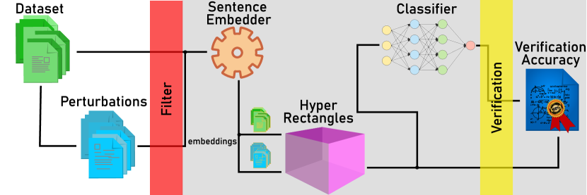
Figure 2: Visualisation of the NLP verification pipeline followed in our approach.

This section presents a parametric NLP verification pipeline, shown in Figure 2 diagrammatically. We call it “parametric” because each component within the pipeline operates independently of the others and can be taken as a parameter when studying other components. The parametric nature of the pipeline allows for the seamless integration of state-of-the-art methods at every stage, and for more sophisticated experiments with those methods. Note that the outlined pipeline can be seen as a filter which can be applied on top of an NLP system or LLM (such as S-BERT and S-GPT) to certify intended DNN behavior for safety-critical input queries. The following section provides a detailed exposition of the methodological choices made at each step of the pipeline.

0.3.1 Semantic Perturbations

As discussed in Section 0.2.5, we require semantic perturbations for creating semantic subspaces. To do so, we consider three kinds of perturbations – i.e. character, word and sentence level. This systematically accounts for different variations of the samples.

Character and word level perturbations

are created via a rule-based method proposed in [91], to simulate different kinds of noise one could expect from spelling mistakes, typos etc. These perturbations are non-adversarial and can be generated automatically. The authors found that NLP models are sensitive to such small errors, while in practice this should not be the case. Character level perturbations types include randomly inserting, deleting, replacing, swapping or repeating a character of the data sample. At the character level, we do not apply letter case changing, given it does not change the sentence-level representation of the sample, nor do we apply perturbations to commonly misspelled words, given only a small overlap of those words occur in our datasets. Perturbations types at the word level include randomly repeating or deleting a word, changing the ordering of the words, the verb tense, singular verbs to plural verbs or adding negation to the data sample. At the word level, we omit replacement with synonyms, as this is accounted for via sentence rephrasing. Negation is not done on the medical safety dataset, as it creates label ambiguities (e.g. ‘pain when straightening knee’ $\rightarrow$ ‘no pain when straightening knee’), as well as singular plural tense and verb tense, given human annotators would experience difficulties with this task (e.g. rephrase the following in plural/ with changed tense – ‘peritonsillar abscess drainage aftercare.. please help’).

Further examples of character and word rule-based perturbations can be found in Tables 3 and 4.

Method	Description	Original sentence	Altered sentence
Insertion	A character is randomly selected and inserted in a random position.	Are you a robot?	Are yovu a robot?
Deletion	A character is randomly selected and deleted.	Are you a robot?	Are you a robt?
Replacement	A character is randomly selected and replaced by an adjacent character on the keyboard.	Are you a robot?	Are you a ronot?
Swapping	A character is randomly selected and swapped with the adjacent right or left character in the word.	Are you a robot?	Are you a rboot?
Repetition	A character in a random position is selected and duplicated.	Are you a robot?	Arre you a robot?

Table 3: Character-level perturbations: their types and examples of how each type acts on a given sentence from the R-U-A-Robot dataset [47]. Perturbations are selected from random words that have 3 or more characters, first and last characters of a word are never perturbed.

Method	Description	Original sentence	Altered sentence
Deletion	Randomly selects a word and removes it.	Can u tell me if you are a chatbot?	Can u tell if you are a chatbot?
Repetition	Randomly selects a word and duplicates it.	Can u tell me if you are a chatbot?	Can can u tell me if you are a chatbot?
Negation	Identifies verbs then flips them (negative/positive).	Can u tell me if you are a chatbot?	Can u tell me if you are not a chatbot?
Singular/ plural verbs	Changes verbs to singular form, and conversely.	Can u tell me if you are a chatbot?	Can u tell me if you is a chatbot?
Word order	Randomly selects consecutive words and changes the order in which they appear.	Can u tell me if you are a chatbot?	Can u tell me if you are chatbot a?
Verb tense	Converts present simple or continuous verbs to their corresponding past simple or continuous form.	Can u tell me if you are a chatbot?	Can u tell me if you were a chatbot?

Table 4: Word-level perturbations: their types and examples of how each type acts on a given sentence from the R-U-A-Robot dataset [47].

Sentence level perturbations.

We experiment with two types of sentence level perturbations, particularly due to the complicated nature of the medical queries (e.g. it is non-trivial to rephrase queries such as this – ‘peritonsillar abscess drainage aftercare.. please help’). We do so by either using Polyjuice [132] or vicuna-13b. Polyjuice is a general-purpose counterfactual generator that allows for control over perturbation types and locations, trained by fine-tuning GPT-2 on multiple datasets of paired sentences. Vicuna is a state-of-the-art open source chatbot trained by fine-tuning LLaMA [115] on user-shared conversations collected from ShareGPT . For Vicuna, we use the following prompt to generate variations on our data samples ‘Rephrase this sentence 5 times: “[Example]”.’ For example, from the sentence “How long will I be contagious?", we can obtain “How many years will I be contagious?" or “Will I be contagious for long?" and so on.

We will use notation $\mathcal{P}$ to refer to a perturbation algorithm abstractly.

0.3.2 NLP Embeddings

Next component of the pipeline are embeddings. Embeddings play a crucial role in NLP verification as they map textual data into continuous vector spaces, in a way that should capture semantic relationships and contextual information.

Given an NLP dataset $\mathcal{Y}$ as a set of sentences $s_{1},\ldots,s_{q}$ written in natural language, an embedding $\mathbb{E}$ is a function that maps a sentence to a vector in ^m. The vector space ^m is called the embedding space. Ideally, $\mathbb{E}$ should reflect the semantic similarities between sentences in $\mathcal{Y}$, i.e. the more semantically similar two sentences $s_{i}$ and $s_{j}$ are, the closer the distance between $\mathbb{E}(s_{i})$ and $\mathbb{E}(s_{j})$ should be in ^m. Of course, defining semantic similarity in precise terms may not be tractable (the number of unseen sentences maybe infinite, the similarity maybe understood subjectively and/or depending on the context). This is why, the state-of-the-art NLP relies on machine learning methods to capture the notion of semantic similarity approximately.

Currently, the most common approach to obtain an embedding function $\mathbb{E}$ is by training transformers [32, 101]. Transformers are a type of DNNs that can be trained to map sequential data into real vector spaces and are capable of handling variable-length input sequences. They can also be used for other tasks, such as classification or sentence generation, but in those cases, too, training happens at the level of embedding spaces. In this work, a transformer is trained as a function $\mathbb{E}:\mathcal{Y}\rightarrow^{m}$ for some given $m$. The key feature of the transformer is the “self-attention mechanism", which allows the network to weigh the importance of different elements in the input sequence when making predictions, rather than relying solely on the order of elements in the sequence. This makes them good at learning to associate semantically similar words or sentences. In this work we initially use Sentence-BERT [101] and later add Sentence-GPT [92] to embed sentences. Unfortunately, the relation between the embedding space and the NLP dataset is not bijective: i.e. each sentence is mapped into the embedding space, but not every point in the embedding space has a corresponding sentence. This problem is well-known in NLP literature [65] and, as shown in this paper, is one of the reasons why verification of NLP is tricky. Given an NLP dataset $\mathcal{Y}$ that should be classified into $n$ classes, the standard approach is to construct a function $N:^{m}\rightarrow^{n}$ that maps the embedded inputs to the classes. In order to do that, a domain specific classifier $N$ is trained on the embeddings $\mathbb{E}(\mathcal{Y})$ and the final system will then be the composition of the two subsystems, i.e. $N\circ\mathbb{E}$.

0.3.3 Geometric Analysis of Embedding Spaces

We now formally define geometric and semantic subpaces of the embedding space. Our goal is to define subpaces on the embedding space ^m by using an effective algorithmic procedure.

We start with an observation that, given an NLP dataset $\mathcal{Y}$ that contains (a finite number of sentences) $s_{1},\ldots,s_{q}$, and an embedding function $\mathbb{E}:\mathcal{Y}\rightarrow^{m}$, we can define an embedding matrix $\mathcal{X}\in^{q\times m}$, where each row $j$ is given by $\mathbb{E}(s_{j})$. Treating embedded sentences as matrices, rather than as points in the real vector space, makes many computations easier. This motivates the following definition of a hyper-rectangle for $\mathcal{X}$.

Definition 1 (Hyper-rectangle for an Embedding Matrix).

Given an embedding matrix $\mathcal{X}\in^{q\times m}$, the $m$-dimensional hyper-rectangle for $\mathcal{X}$ is defined as:

$$\mathbb{H}_{\mathcal{X}}\coloneqq\{x\in^{m}:\forall j\in[1,...,m].\>x^{j}\in[\min\nolimits_{i}(\mathcal{X}^{ij}),\max\nolimits_{i}(\mathcal{X}^{ij})]\}.$$

where $\min\nolimits_{i}(\mathcal{X}^{ij})$ stands for the minimum value of the $j$-th element $x^{j}$ across all rows $i\in\{0,\ldots,q\}$ in $\mathcal{X}$; similarly for $\max\nolimits_{i}(\mathcal{X}^{ij})$.

Definition 2 (Subspace of the Embedding Space).

Given a NLP dataset $\mathcal{Y}$, an embedding function $\mathbb{E}:\mathcal{Y}\rightarrow^{m}$, and $\mathcal{Y}^{\prime}\subseteq\mathcal{Y}$ (with $\mathcal{Y}^{\prime}=\{s_{1},\ldots,s_{q}\}$), we say a hyper-rectangle $\mathbb{H}_{\mathcal{X}^{\prime}}$ is a subspace of the embedding space ^m around $\mathcal{Y}^{\prime}$ if the matrix $\mathcal{X}^{\prime}\in^{q\times m}$ satisfies the following condition: each $j$th row is given by $\mathbb{E}(s_{j})$.

We will use notation $\mathcal{S}$ to refer to a subspace. The next example shows how the above definitions generalise the commonly known definition of the $\epsilon\text{-cube}$.

Example 1 ($\epsilon\text{-cube}$ and $\epsilon\text{-ball}$).

One of the most popular terms used in robust training [45] and verification[22] literature is the $\epsilon\text{-ball}$. It is defined as follows. Given one row $\hat{x}$ from $\mathcal{X}$, a constant $\epsilon\in$, and a distance function (L-norm) $||-||$ the $\epsilon\text{-ball}$ around $\hat{x}$ of radius $\epsilon$ is defined as:

$$\mathbb{B}(\hat{x},\epsilon)\coloneqq\{x\in^{m}:||\hat{x}-x||\leq\epsilon\}.$$

In practice, it is common to use the $L_{\infty}$ norm, which results in the $\epsilon\text{-ball}$ actually being a hyper-rectangle, also called $\epsilon\text{-cube}$. To see this, take the construction of $\mathbb{H}_{\mathcal{X}}$, and define $\mathcal{X}\in^{2\times m}$ where the first row is given by $\hat{x}_{j}=\hat{x}_{j}+\epsilon$ for each element $\hat{x}_{j}$ of $\hat{x}$, and the second row is given by $\hat{x}_{j}=\hat{x}_{j}-\epsilon$.

We will use notation $\mathbb{H}_{\epsilon}$ to refer to an $\epsilon\text{-cube}$ (assuming that the choice of $\hat{x}$ is clear from the context).

Of course, as we have already discussed in the introduction and Figure 1, hyper-rectangles are not very precise, geometrically. A more precise shape would be a convex hull around $q$ given points in the embedding space. Indeed literature has some definitions of convex hulls [7, 105, 55]. However, none of them is suitable as they are computationally too expensive due to the time complexity of $O(q^{m/2})$ where $q$ is the number of inputs and $m$ is the number of dimensions [7]. Approaches that use under-approximations to speed up the algorithms [105, 55] do not work well in NLP scenarios, as under-approximated subspaces are so small that they contain near zero sentence embeddings.

A computationally efficient way of making hype-rectangles more precise is to rotate them to align to the position of the given points in the embedding space. This motivates us to introduce the Eigenspace rotation.

Eigenspace Rotation.

To construct the tightest possible hyper-rectangle, we define a specific method of eigenspace rotation. As shown in Figure 1 (C and D), our approach is to calculate a rotation matrix $A$ such that the rotated matrix $\mathcal{X}_{\text{rot}}=\mathcal{X}A$ is better aligned with the axes than $\mathcal{X}$, and therefore $\mathbb{H}_{\mathcal{X}_{\text{rot}}}$ has a smaller volume. By a slight abuse of terminology, we will refer to $\mathbb{H}_{\mathcal{X}_{\text{rot}}}$ as the rotated hyper-rectangle, even though strictly speaking, we are rotating the data, not the hyper-rectangle itself. In order to calculate the rotation matrix $A$, we use singular value decomposition [60]. The singular value decomposition of $\mathcal{X}$ is defined as $\mathcal{X}=U\Sigma V^{*}$, where $U$ is a matrix of left-singular vectors, $\Sigma$ is a matrix of singular values and $V^{*}$ is a matrix of right-singular vectors and $\cdot^{*}$ denotes the conjugate transpose. Intuitively, the right-singular vectors $V^{*}$ describe the directions in which $\mathcal{X}$ exhibits the most variance. The main idea behind the definition of rotation is to align these directions of maximum variance with the standard canonical basis vectors. Formally, using $V^{*}$, we can compute the rotation (or change-of-basis) matrix $A$ that rotates the right-singular vectors onto the canonical standard basis vectors $I$, where $I$ is the identity matrix. To do this, we observe that $V^{*}A=I\rightarrow V^{*}=IA^{-1}\rightarrow V^{-1}=A^{-1}\rightarrow V=A$. We thus obtain $\mathcal{X}_{rot}=\mathcal{X}A$ as desired.

All hyper-rectangles constructed and used in this paper are rotated.

Geometric and Semantic Subspaces.

We now apply the abstract definition of a subspace of an embedding space to concrete NLP verification scenarios. Once we know how to define subspaces for a selection of points in the embedding space, the choice remains how to choose those points. The first option is to use $\epsilon\text{-cubes}$ around given embedded points, as Example 1 defines. Since this construction does not involve any knowledge about the semantics of sentences, we will call the resulting subspaces geometric subspaces. The second choice is to apply semantic perturbations to a point in $\mathcal{Y}$, embed the resulting sentences, and then define a subspace around them. We will call the subspaces obtained by this method semantic perturbation subspaces, or just semantic subspaces for short.

We will finish this section with defining semantic subspaces formally. Given a data set $\mathcal{Y}$, and some defined algorithm for sentence perturbation $\mathcal{P}$, we can form $\mathcal{Y}^{\prime}=\{s^{*}_{1},\ldots,s^{*}_{q}\}$, such that each $s^{*}_{i}=\mathcal{P}(s_{i})$. Intuitively, we want to construct a subspace for $\mathcal{Y}^{\prime}$ as described in Definition 2. However, in the later sections, we will need to refer to different kinds of perturbations (e.g. character, word or sentence level as explained in Section 0.3.1) or different types of perturbations (e.g. insertion, deletion, replacement, etc.) as illustrated in Tables 3 and 4). This motivates the following definitions. Notation $\mathcal{P}_{k}^{t}(s,a)$ will denote a perturbation of kind $k$ and type $t$, applied in the sentence $s$, in a position $a$. As all algorithms we use choose $a$ randomly, we will omit $a$ and write just $\mathcal{P}_{k}^{t}(s)$. When we say that a sentence $s$ has $b$ semantic perturbations of kind $k$, we refer to a set $\mathcal{A}^{k}_{s}=\{\mathcal{P}_{k}^{t_{1}}(s),\mathcal{P}_{k}^{t_{2}}(s),\ldots,\mathcal{P}_{k}^{t_{b}}(s)\}$, for some given choice of $b$ perturbations of types $t_{1},\ldots,t_{b}$. When the choice is unimportant or clear from the context, we may omit mentioning the chosen types of perturbation.

Definition 3 (Semantic Subspace for a Sentence).

Suppose we are given an NLP dataset $\mathcal{Y}=\{s_{1},\ldots,s_{q}\}$, and an embedding function $\mathbb{E}:\mathcal{Y}\rightarrow^{m}$.

Given a sentence $s_{i}$ and a corresponding set $\mathcal{A}^{k}_{s_{i}}$ of its semantic perturbations (of kind $k$), a semantic subspace for $s_{i}$ is a subspace around $\mathcal{Y}^{\prime}=\mathcal{A}^{k}_{s_{i}}$ constructed according to Definition 2.

It will be useful in the later sections to use notation $\mathbb{H}_{\mathcal{X}_{s_{i}}}$ to refer to the hyper-rectangle used in constructing the semantic subspace for $s_{i}$. We will refer to a set of such hyper-rectangles $\mathbb{H}^{*}_{k}=\bigcup_{i=1}^{q}\mathbb{H}^{*}_{\mathcal{X}_{s_{i}}}$, where $s_{i}\in\{s_{1},\ldots,s_{q}\}$ and $k$ is a chosen perturbation kind.

If $\mathbb{H}^{*}_{k}$ is based on perturbations of only one type, we will sometimes use that type as an index to $\mathbb{H}^{*}_{\_}$.

Example 2 (Construction of Semantic Subspaces).

To illustrate this construction, let us consider the sentence $s_{i}=$“Can u tell me if you are a chatbot?”. This sentence is one of $3400$ original sentences of the positive class in the dataset. From this single sentence, we can create six sentences (word-level perturbations), see Table 4. Once these seven sentences are embedded into the vector space, they form the hyper-rectangle $\mathbb{H}_{\mathcal{X}_{s_{i}}}$. By repeating this construction for the remaining $3399$ sentences, we obtain the set of hyper-rectangles $\mathbb{H}^{*}_{word}$ for the dataset.

0.3.4 Training

As outlined in Section 0.2.2, robust training is essential for bolstering the robustness of DNNs; without it, their verifiability would be significantly diminished. This study employs two robust training methods, namely data augmentation and a custom PGD adversarial training, with the goal of discerning the factors contributing to the success of robust training and compare the effectiveness of these methods.

Data Augmentation.

In this training method, we statically generate semantic perturbations at the character, word, and sentence levels before training, which are then added to the dataset. The network is subsequently trained on this augmented dataset using the standard stochastic gradient descent algorithm.

Adversarial Training.

In this training method, we modify the traditional Projected Gradient Descent (PGD) algorithm [85], defined as follows. Given a loss function $\mathcal{L}$, a step size $\gamma\in$ and a starting point $\hat{x}_{0}$ then the output of the PGD algorithm $x(l)$ after $l$ iterations is defined as:

$$x(0) =\hat{x}_{0}$$

$$x(t+1) =\text{proj}_{\mathbb{H}}\Big{[}x(t)+\gamma\cdot\text{sign}(\nabla_{x(t)}\mathcal{L}(x(t),y))\Big{]}$$

where $\text{proj}_{\mathbb{H}}$ is the projection back into the desired subspace $\mathbb{H}$. In its standard formulation, the subspace $\mathbb{H}$ is often an $\epsilon\text{-ball}$ (for some chosen $\epsilon$). In this work, we modify the algorithm to work with custom-defined hyper-rectangles as the subspace.

The primary distinction between our customised PGD algorithm and the standard version lies in the definition of the step size. In the conventional algorithm, the step size is represented by a scalar $\gamma\in$, whereas in our adaptation, it transforms into a vector $\gamma\in^{m}$, where $m$ denotes the size of the input space. Note that the dot product $\cdot$ between $\gamma$ and the sign of the gradient $sign(\nabla)$ becomes an element-wise multiplication. This modification allows us to account for the varying sizes of each dimension of the given hyper-rectangle, contrasting with the uniform size of all $\epsilon\text{-balls}$ in the standard approach.

The resulting customised PGD training seeks to identify the worst perturbations within the custom-defined subspace, and trains the given neural network to classify those perturbations correctly, in order to make the network robust to adversarial inputs in the chosen subspace.

0.3.5 Choice of Verification Algorithm

As stated earlier, our approach in this study involves the utilization of cutting-edge tools for DNN verification. Initially, we employ ERAN [110], a state-of-the-art abstract interpretation-based method. This choice is made over IBP due to its ability to yield tighter bounds. Subsequently, we conduct comparisons and integrate Marabou [131], a state-of-the-art complete and precise SMT-based verifier. This enables us to attain the highest verification percentage, maximizing the tightness of the bounds.

We will use notation $\mathcal{V}$ to refer to a verifier abstractly.

0.4 Characterisation of Verifiable Subspaces

In this Section, we provide key results in support of Contribution 1 formulated in the introduction:

• We start with introducing the metric of generalisability of (verified) subspaces, and introducing the problem of the generalisability-verifiability trade-off.

• We show that the use of semantic subspaces helps to find a better balance between generalisability and verifiability, as compared to the use of geometric subspaces.

• Finally, we show that adversarial training based on semantic subspaces results in DNNs that are both more verifiable and more generalisable than those obtained with other forms of robust training.

0.4.1 Generalisability-Verifiability Trade-off

This subsection defines the new metric of generalisability and shows its effect on (naively defined) geometric subspaces.

Generalisability of Verified Subspaces: Formal Definition

Let us start with recalling the existing standard metrics used in DNN verification. Recall that we are given an NLP dataset $\mathcal{Y}=\{s_{1},\ldots,s_{q}\}$, moreover we assume that each $s_{i}$ is assigned a correct class from $C=\{c_{1},\ldots,c_{n}\}$. We restrict to the case of binary classification in this paper for simplicity, so we will assume $C=\{c_{1},c_{2}\}$. Furthermore, we are given an embedding function $\mathbb{E}:\mathcal{Y}\rightarrow^{m}$, and a DNN $N:^{m}\rightarrow^{n}$. Usually $n$ corresponds to the number of classes, and thus in case of binary classification, we have $N:^{m}\rightarrow^{2}$. Classification, or assignment of a vector $v$ in ^m to a class, depends on the highest value in the vector $N(v)$. The most popular metric is accuracy of $N$, which is measured as a percentage of $q$ vectors in ^m that are assigned to a correct class by $N$. Note that this metric checks a finite number of points in ^m given by the data set.

The most popular metric in DNN verification is verifiability. Recall that we can define subspaces $\{\mathcal{S}_{1},\ldots,\mathcal{S}_{s}\}$ of ^m; in such a way that each of them is associated with a class (to which all points in that subspace should belong). A DNN verifier $\mathcal{V}$ takes an $\mathcal{S}_{i}$, its designated class $c_{i}$ and $N$ as an input, and returns as an output an answer whether all points in $\mathcal{S}_{i}$ are guaranteed to be assigned to the class $c_{i}$ by $N$. Verifiability is a percentage of subspaces in $\{\mathcal{S}_{1},\ldots,\mathcal{S}_{s}\}$ that are successfully verified. All DNN verification papers report this measure. Note that each $\mathcal{S}_{i}$ contains an infinite number of points.

We are introducing a third metric – generalisability of (verified) subspaces. Suppose we have a subspace $\mathcal{S}_{i}$ that verifiably consists only of vectors that are assigned to a class $c_{i}$ by $N$. Because of the embedding gap, we cannot know in advance how many valid sentences in $\mathcal{Y}$ (or outside of $\mathcal{Y}$ !) will be mapped into $\mathcal{S}_{i}$ by $\mathbb{E}$. Checking the former is rather easy, but may not reflect the idea of generalisability to unseen similar sentences. Checking the latter is hard. We propose the following effective heuristic. By the constructions of the previous section, any $\mathcal{S}_{i}$ necessarily contains an embedding of at least one element $s_{i}$ from $\mathcal{Y}$. Choosing any perturbation algorithm $\mathcal{P}$ (of kind $k$), we can form a set $\mathcal{A}^{k}_{s_{i}}$, as described in Section 0.3.3. Note that $\mathcal{P}$ (and $k$) can be given by a collection of different perturbation algorithms and their kinds. The key assumption is that $\mathcal{A}^{k}_{s_{i}}$ contains valid sentences semantically similar to $s_{i}$ and belonging to the same class.

Consider a set $\mathcal{V}_{i}$ of vectors in ^m such that each vector $v_{j}\in\mathcal{V}_{i}$ is defined as $v_{j}=\mathbb{E}(s_{j})$, with $s_{j}\in\mathcal{A}^{k}_{s_{i}}$. This is the set of embeddings of sentences contained in $\mathcal{A}^{k}_{s_{i}}$. Percentage of elements of $\mathcal{V}_{i}$ contained in $\mathcal{S}_{i}$ gives us the generalisability of $\mathcal{S}_{i}$. Note that each $\mathcal{V}_{i}$ is finite, because each $\mathcal{A}^{k}_{s_{i}}$ is finite.

Note that, unlike accuracy and verifiability, the generalisability metric does not explicitly depend on any DNN. However, in this paper we only study generalisability of verifiable subspaces, and thus the existence of a verified DNN $N$ will be assumed.

Because verifiability is reported as a percentage of $\{\mathcal{S}_{1},\ldots,\mathcal{S}_{s}\}$, it will be convenient to report generalisability over the set of subspaces $\mathcal{S}=\bigcup\mathcal{S}_{i}$. For this, we take $\mathcal{A}=\bigcup\mathcal{A}^{k}_{s_{i}}$ and the corresponding $\mathcal{V}=\bigcup\mathcal{V}_{i}$ for all $s_{i}\in\mathcal{Y}$ and compute generalisability of $\mathcal{S}$ as a percentage of elements of $\mathcal{V}$ contained in all subspaces of $\mathcal{S}$. When it is important to emphasise the kind of perturbation, we will use the notation $\mathcal{A}_{k}$ for $\bigcup\mathcal{A}^{k}_{s_{i}}$.

Base Line Experiments: Understanding the Properties of Embedding Spaces

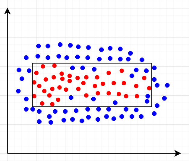
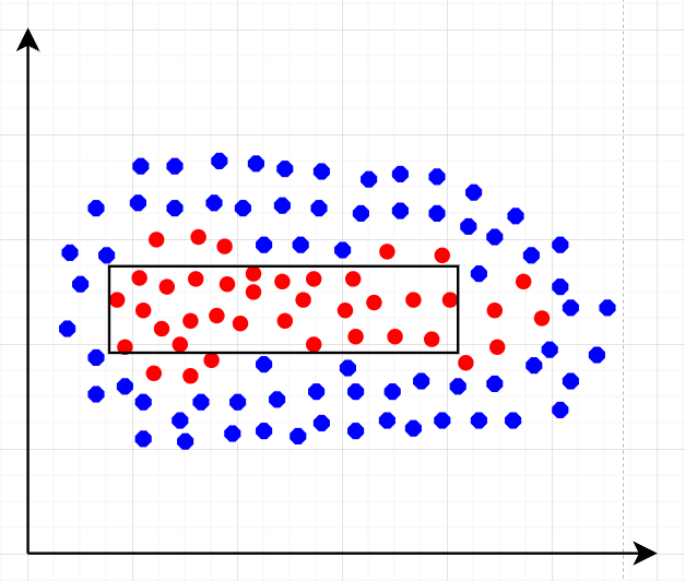
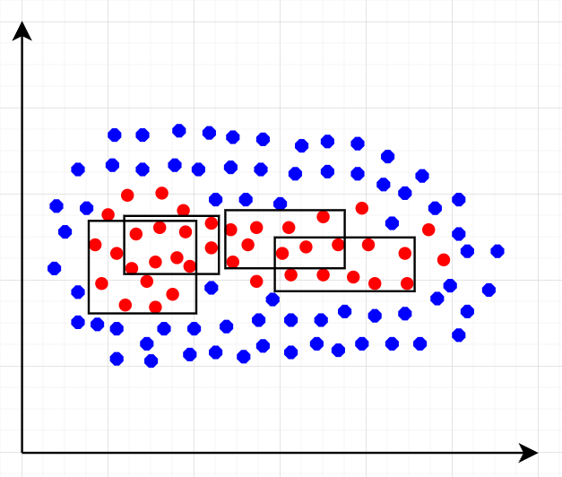
Figure 3: An example of hyper-rectangle drawn around all points of the same class (left), shrunk hyper-rectangle $\mathbb{H}_{sh}$ that is obtained by excluding all points from the opposite class (center) and clustered hyper-rectangles (right) in 2-dimensions. The red dots represent sentences in the embedding space of one class, while the blue dots are embedded sentences that do not belong to that class.

The methodology defined thus far has given basic intuitions about the relative nature of the NLP verification pipeline. Bearing this in mind, it is important to start our analysis with the general study of the embedding (sub)spaces and suitable base line settings.

Benchmark data sets will be abbreviated as “RUAR" and “Medical". For a benchmark network $N:^{m}\rightarrow^{2}$, we train a medium-sized fully-connected DNN, using stochastic gradient descent and cross-entropy loss. The main requirement for a benchmark network is its sufficient accuracy, see Table 5.

Model	Adversarial training	Train Accuracy RUAR	Test Accuracy RUAR	Train Accuracy Medical	Test Accuracy Medical
$N_{base}$	No	0.9387 ± 0.0014	0.9357 ± 0.0018	0.9632 ± 0.0005	0.9449 ± 0.0026

Table 5: Accuracy of the baseline DNN on the R-U-A-Robot and the Medical datasets.

For the choice of subspaces, which is our main interest in this paper, two extreme (and trivially defined) benchmarks, are the following geometric subspaces:

• a subspace drawn around all embedded sentences of the same class in $\mathcal{Y}$. This is the largest subspace one may wish to verify but we should assume that verifiability of such a subspace would be near $0\%$. It is illustrated in the first graph of Figure 3.

• a collection of subspaces given by very small $\epsilon\text{-cube}$ around each point in $\mathcal{Y}$ (sufficiently small to give very high verifiability). This is illustrated in the first graph of Figure 1.

We need to first understand exact geometric properties (e.g. volume, $\epsilon$ values) and exact verifiability figures for these two extremes. Let us start with understanding the volumes.

Volumes of Subspaces.

To start with the largest hyper-rectangle, we need to ensure that it is shrunk to exclude all samples from $\mathcal{Y}$ from the wrong class. We define the shrinking method that involves reducing the size of the hyper-rectangle to eliminate each input within the hyper-rectangle that does not pertain to the chosen class. Second graph of Figure 3 gives a visual intuition of how this is done.

Formally, suppose we have a hyper-rectangle $\mathbb{H}_{\mathcal{X}}$ and a vector $\hat{x}\in\mathbb{H}_{\mathcal{X}}$ that violates the class requirement. Recall that by definition:

$$\mathbb{H}_{\mathcal{X}}\coloneqq\{x\in^{m}:\forall j\in[1\;,\;...\;,\;m]\;.\;\>x^{j}\in[\min\nolimits_{i}(\mathcal{X}^{ij}),\;\;\max\nolimits_{i}(\mathcal{X}^{ij})]\}.$$

The algorithm starts with choosing a dimension $j\in[1,...,m]$, and computing whether $|\hat{x}^{j}-\min\nolimits_{i}(\mathcal{X}^{ij})|\leq|\hat{x}^{j}-\max\nolimits_{i}(\mathcal{X}^{ij})|$. If the inequality holds, take $d_{\min\nolimits}=|\hat{x}^{j}-\min\nolimits_{j}(\mathcal{X}^{ij})|$ and compute a new minimum for the dimension $j$: $\min\nolimits^{new}_{i}(\mathcal{X}^{ij})=\min\nolimits_{i}(\mathcal{X}^{ij})+d_{min}+\delta$, where $\delta$ is a small positive number (we use $e^{-100}$). We then recompute $\mathbb{H}_{sh}=\mathbb{H}_{\mathcal{X}}$ with $\min\nolimits_{i}(\mathcal{X}^{ij})=\min\nolimits^{new}_{i}(\mathcal{X}^{ij})$ for the chosen dimension $j$.

If the inequality does not hold, take $d_{\max\nolimits}=|\hat{x}^{j}-\max\nolimits_{i}(\mathcal{X}^{ij})|$ and compute a new maximum for the dimension $j$: $\max\nolimits^{new}_{i}(\mathcal{X}^{ij})=\max\nolimits_{i}(\mathcal{X}^{ij})-d_{max}-\delta$, with $\delta$ defined as above. We then recompute $\mathbb{H}_{sh}=\mathbb{H}_{\mathcal{X}}$ with $\max\nolimits_{i}(\mathcal{X}^{ij})=\max\nolimits^{new}_{i}(\mathcal{X}^{ij})$ for the chosen dimension $j$.

Note that modifying just one dimension of $\hat{x}$ like this guarantees that it is not in $\mathbb{H}_{sh}$. The algorithm we apply when computing $\mathbb{H}_{sh}$ involves a heuristic for choosing the optimal dimension along which we modify the hyper-rectangle. The idea is to make the most conservative choice, that excludes as few other embedded sentences as possible. It amounts to computing how many inputs from the chosen class remain inside of the hyper-rectangle after applying the shrinking algorithm to one $j\in[1,...,m]$ at a time, separately. We choose the dimension $j$ for which the hyper-rectangle retains the most inputs of the correct class. The algorithm is run iteratively for every element of $\mathbb{H}_{sh}$ that has the wrong class, until $\mathbb{H}_{sh}$ contains only embeddings of sentences of one class.

For the smallest benchmark subspace, we take $\epsilon\text{-cube}$ of size $\epsilon=0.005$. One $\epsilon\text{-cube}$ around (the embedding of) an arbitrary sentence in $\mathcal{Y}$ will be denoted as $\mathbb{H}_{\epsilon=0.005}$. When taking a collection of hyper-rectangles around all sentences in $\mathcal{Y}$, we obtain a set we denoted as $\mathbb{H}^{*}_{\epsilon=0.005}$.

Generally, we use the following notation: if $\mathbb{H}_{m}$ denotes a hyper-rectangle obtained using a method $m$, then $\mathbb{H}^{*}_{m}$ refers to the union of all hyper-rectangles that can be constructed using $m$ for all elements of the given data set. For example, R-U-A-Robot dataset contains $3400$ sentences of the positive class, and therefore $3400$ $\epsilon\text{-cubes}$ constitute $\mathbb{H}^{*}_{\epsilon=0.005}$ for this dataset. We will say that $3400$ is the cardinality of $\mathbb{H}^{*}_{\epsilon=0.005}$.

To give us a sense of progression from the largest hyper-rectangle to the smallest, we also cluster $\mathbb{H}_{sh}$, see the last graph of Figure 3. For the clustering method, we employ the k-means algorithm to generate multiple ensembles of hyper-rectangles around each cluster. This approach guarantees that the hyper-rectangles contain solely points from the specific class, while also reducing their volume. We obtain a set of $50$, $100$, $200$, $250$ clusters denoted as $\mathbb{H}^{*}_{50}$ – $\mathbb{H}^{*}_{250}$.

Table 6 shows average volumes of the subspaces that we obtain, for two data sets. Notice consistent reduction of volume, from $\mathbb{H}_{sh}$ to $\mathbb{H}^{*}_{50}$ - $\mathbb{H}^{*}_{250}$ and ultimately to $\mathbb{H}^{*}_{\epsilon=0.005}$. There are several orders of magnitude between the largest and the smallest subspace.

Hyper-rectangles	Construction method	Avg. volume of $\mathbb{H}$ RUAR	Set cardinality of $\mathbb{H}^{*}$ RUAR	Avg. volume of $\mathbb{H}$ Medical	Set cardinality of $\mathbb{H}^{*}$ Medical
$\mathbb{H}_{sh}$	Hyper-rectangle shrunk to exclude all negative examples	7.55e-11	1	2.6e-09	1
$\mathbb{H}^{*}_{50}$	Set of hyper-rectangles on 50 clusters	1.02e-16	50	6.56e-15	50
$\mathbb{H}^{*}_{100}$	Set of hyper-rectangles on 100 clusters	6.23e-18	100	3.25e-17	100
$\mathbb{H}^{*}_{200}$	Set of hyper-rectangles on 200 clusters	3.31e-20	200	4.67e-19	200
$\mathbb{H}^{*}_{250}$	Set of hyper-rectangles on 250 clusters	6.42e-22	250	2.42e-20	250
$\mathbb{H}^{*}_{\epsilon=0.005}$	Set of $\epsilon$-cubes around all positive dataset sentences, $\epsilon=0.005$	1.00e-60	3400	1.00e-60	989

Table 6: Sets of geomtetric subspaces used in the experiments, their cardinality and average volumes of hyper-rectangles. All shapes are eigenspace rotated for better precision.

Verifiability Range for Subspaces.

For each set of hyper-rectangles and the given network, we pass them to the verifier (ERAN) and measure verifiability. Table 7 shows that the shrunk hyper-rectangle $\mathbb{H}_{sh}$ achieves zero verifiability, and the various clustered hyper-rectangles ($\mathbb{H}^{*}_{50}$, $\mathbb{H}^{*}_{100}$ $\mathbb{H}^{*}_{200}$, $\mathbb{H}^{*}_{250}$) achieve at most negligible verifiability. We call this effect low verifiability of the subspaces. In contrast, the baseline $\mathbb{H}^{*}_{\epsilon=0.005}$ achieves up to $99.60\%$ verifiability. This suggests that $\epsilon=0.005$ is a good benchmark for a different extreme. Table 6 can give us an intuition of why $\mathbb{H}^{*}_{\epsilon=0.005}$ has notably higher verifiability than the other hyper-rectangles: the volume of $\mathbb{H}^{*}_{\epsilon=0.005}$ is several orders of magnitude smaller.

Dataset	Model	$\boldsymbol{\mathbb{H}_{sh}}$	$\boldsymbol{\mathbb{H}^{*}_{50}}$	$\boldsymbol{\mathbb{H}^{*}_{100}}$	$\boldsymbol{\mathbb{H}^{*}_{200}}$	$\boldsymbol{\mathbb{H}^{*}_{250}}$	$\boldsymbol{\mathbb{H}^{*}_{\epsilon=0.05}}$	$\boldsymbol{\mathbb{H}^{*}_{\epsilon=0.005}}$
RUAR	$N_{base}$	0.00	0.00	1.33	0.52	0.41	0.00	88.67
Medical	$N_{base}$	0.00	0.00	0.00	2.10	4.08	5.00	97.86

Table 7: Verifiability of the baseline DNN on the R-U-A-Robot and the Medical datasets, for a selection of geometric subspaces; for ERAN verifier.

Verifiability-Generalisability Trade-off for Geometric Subspaces

Tables 6 and 7 suggest that smaller subspaces are more verifiable. One may also conjecture that they are less generalisable (as they will contain fewer embedded sentences). We confirm this via experiments; we are particularly interested in understanding how quickly generalisability deteriorates as verifiability increases.

To test generalisability, for each data set, we algorithmically generate a new data set $\mathcal{A}$ containing its semantic perturbations, using the method described in Section 0.3.1. It will be convenient to refer to parts of that set that correspond to perturbations of sentences belonging to positive and negative classes, respectively. In such cases, we will be using the notation $\mathcal{A}^{pos}$ and $\mathcal{A}^{neg}$. Note that in this section, we will work only with $\mathcal{A}^{pos}$. This choice is motivated by the nature of the chosen data sets: both Medical and R-U-A-Robot sentences split into:

• a positive class, that contains sentences with one intended semantic meaning (they are medical queries, or they are questions about robot identity); and

• a negative class that represents “all other sentences". These “other sentences" are not grouped by any specific semantic meaning and therefore do not form one coherent semantic category.

However Section 0.5 will make use of $\mathcal{A}^{neg}$ in the context of falsifiability of verified subspaces.

For the perturbation algorithm $\mathcal{P}$, in this experiment we take a combination of different perturbations algorithms. For R-U-A-Robot, $\mathcal{P}_{RUAR}=\{$ character insertion, character deletion, character replacement, character swapping, character repetition, word deletion, word repetition, word negation, word singular/plural verbs, word order, word tense $\}$. For the Medical dataset, $\mathcal{P}_{Medical}=\{$ character insertion, character deletion, character replacement, character swapping, character repetition, word deletion, word repetition, word negation, word singular/plural verbs, word order, word tense, sentence polyjuice $\}$. Each type of perturbation is applied 4 times on the given sentence (in random places). The resulting data sets of semantic perturbations $\mathcal{A}^{pos}_{RUAR}$ and $\mathcal{A}^{pos}_{medical}$ are approximately two orders of magnitude larger than the original data sets (see Table 8), and contain so far unseen sentences of similar semantic meaning to the ones present in the original data sets $RUAR$ and $Medical$.

For generalisability, Table 8 shows that the most verifiable subspace $\mathbb{H}^{*}_{\epsilon=0.005}$ is the least generalisable. This means $\mathbb{H}^{*}_{\epsilon=0.005}$ may not contain any valid new sentences apart from the one for which it was formed! At the same time, $\mathbb{H}^{*}_{\epsilon=0.05}$ has up to $48\%$ of generalisability at the expense of only up to $5\%$ of verifiability (cf. Table 7). The effect of the generalisability vs verifiability trade-off can thus be rather severe for geometric subspaces.

This experiment demonstrates the importance of using the generalisability metric, as with only taking into account the verifiability of the subspaces one would choose $\mathbb{H}^{*}_{\epsilon=0.005}$, obtaining mathematically sound but pragmatically useless results. We argue that this is a strong argument for including generalisability as a standard metric in reporting NLP verification results in the future.

Dataset	Hyper-rectangles	Avg. Volume of $\mathbb{H}$	Generalisability (%)	Generalisability (# of sentences)	Total Sentences in $\mathcal{A}^{pos}$
RUAR	$\mathbb{H}^{*}_{\epsilon=0.005}$	1.00e-60	1.95	2821	144500
	$\mathbb{H}^{*}_{\epsilon=0.05}$	1.00e-30	38.47	55592	144500
	$\mathbb{H}_{sh}$	7.55e-11	50.91	73561	144500
Medical	$\mathbb{H}^{*}_{\epsilon=0.005}$	1.00e-60	0.09	10	11209
	$\mathbb{H}^{*}_{\epsilon=0.05}$	1.00e-30	28.49	3194	11209
	$\mathbb{H}_{sh}$	2.6e-09	37.13	4162	11209

Table 8: Generalisability of the selected geometric subspaces $\mathbb{H}^{*}_{\epsilon=0.005}$, $\mathbb{H}^{*}_{\epsilon=0.05}$ and $\mathbb{H}_{sh}$, measured on the sets of semantic perturbations $\mathcal{A}^{pos}_{RUAR}$ and $\mathcal{A}^{pos}_{medical}$.

0.4.2 Semantic Subspaces and Generalisability-Verifiability Trade-off

The previous subsection has shown that the generalisability-verifiability trade-off is not resolvable by geometric manipulations alone. In this section we argue that using semantic subspaces can help to improve the effects of the trade-off. The main hypothesis that we are testing is: semantic subspaces permit drawing more precise shapes, and this in turn must improve both verifiability and generalisability.

Verifiability of Semantic Subspaces

We will use the construction given in Definition 3. As Table 9 illustrates, we construct several semantic hyper-rectangles on sentences of the positive class using character-level ($\mathbb{H}^{*}_{char}$, $\mathbb{H}^{*}_{del.}$, $\mathbb{H}^{*}_{ins.}$, $\mathbb{H}^{*}_{rep.}$, $\mathbb{H}^{*}_{repl.}$, $\mathbb{H}^{*}_{swap.}$), word-level ($\mathbb{H}^{*}_{word}$) and sentence-level perturbations ($\mathbb{H}^{*}_{pj}$). The subscripts _char and _word refer to the kind of perturbation algorithm, while _del., _ins., _rep., _repl., _swap. and _pj refer to the type of perturbation, where pj stands for Polyjuice (see Section 0.3.1). Notice comparable volumes of all these shapes, and compare with $\mathbb{H}^{*}_{\epsilon=0.05}$.

Hyper-rectangles	Construction method	Avg. volume of $\mathbb{H}$ RUAR	Set cardinality of $\mathbb{H}^{*}$ RUAR	Avg. volume of $\mathbb{H}$ Medical	Set cardinality of $\mathbb{H}^{*}$ Medical
$\mathbb{H}^{*}_{char}$	Set of hyper-rectangles for character perturbations	1.54e-30	3400	7.66e-31	989
$\mathbb{H}^{*}_{word}$	Set of hyper-rectangles for word perturbations	1.28e-30	3400	-	-
$\mathbb{H}^{*}_{pj}$	Set of hyper-rectangles for polyjuice sentence perturbations	-	-	2.01e-28	989
$\mathbb{H}^{*}_{swap.}$	Set of hyper-rectangles for swapping perturbations	1.57e-31	3400	3.42e-31	989
$\mathbb{H}^{*}_{repl.}$	Set of hyper-rectangles for replacement perturbations	9.84e-31	3400	3.43e-31	989
$\mathbb{H}^{*}_{del.}$	Set of hyper-rectangles for deletion perturbations	3.46e-31	3400	1.24e-32	989
$\mathbb{H}^{*}_{ins.}$	Set of hyper-rectangles for insertion perturbations	3.21e-31	3400	9.11e-33	989
$\mathbb{H}^{*}_{rep.}$	Set of hyper-rectangles for repetition perturbations	1.56e-31	3400	1.06e-32	989
$\mathbb{H}^{*}_{\epsilon=0.05}$	Set of $\epsilon$-cubes generated to match the volume of the hyper-rectangles	1e-30	3400	1e-30	989

Table 9: Sets of semantic subspaces used in the experiments, their cardinality and average volumes of hyper-rectangles. All shapes are eigenspace rotated for better precision.

We pass each set of hyper-rectangles and the network $N_{base}$ to the verifiers ERAN and Marabou to measure verifiability of the subspaces. Table 10 illustrates the verification results obtained using ERAN. From the table, we can infer that the verifiability of our semantic hyper-rectangles is indeed higher than that of the geomtrically-defined hyper-rectangles (Table 7). Furthermore, our semantic hyper-rectangles, while unable to reach the verifiability of $\mathbb{H}^{*}_{\epsilon=0.005}$, achieve notable higher verification than its counterpart of comparable volume $\mathbb{H}^{*}_{\epsilon=0.05}$. From this experiment, we conclude that not only volume, but also precision of the subspaces has an impact on their verifiability.

Dataset	Model	$\boldsymbol{\mathbb{H}^{*}_{\epsilon=0.05}}$	$\boldsymbol{\mathbb{H}^{*}_{word}}$	$\boldsymbol{\mathbb{H}^{*}_{char}}$	$\boldsymbol{\mathbb{H}^{*}_{del.}}$	$\boldsymbol{\mathbb{H}^{*}_{ins.}}$	$\boldsymbol{\mathbb{H}^{*}_{rep.}}$	$\boldsymbol{\mathbb{H}^{*}_{repl.}}$	$\boldsymbol{\mathbb{H}^{*}_{swap.}}$	$\boldsymbol{\mathbb{H}^{*}_{pj}}$
RUAR	$N_{base}$	0.00	1.80	0.87	1.62	2.63	1.66	0.94	2.07	-
Medical	$N_{base}$	5.00	-	39.71	39.62	44.66	48.71	37.49	42.60	50.09

Table 10: Verifiability of the baseline DNN on the R-U-A-Robot and the Medical datasets, for a slection of semantic subspaces; for ERAN verifier.

Following these results, Table 11 reports the verification results using Marabou instead of ERAN. As shown, Marabou is able to verify up to $66.83\%$ ($\mathbb{H}^{*}_{rep.}$), while ERAN achieves at most $50.09\%$. This shows that complete and precise verification (Marabou) outperforms abstract interpretation (ERAN). Overall, the Marabou experiment confirms the trends of improved verifiability shown by ERAN and thus confirms our hypothesis about importance of shape precision.

Dataset	Model	$\boldsymbol{\mathbb{H}^{*}_{\epsilon=0.05}}$	$\boldsymbol{\mathbb{H}^{*}_{word}}$	$\boldsymbol{\mathbb{H}^{*}_{char}}$	$\boldsymbol{\mathbb{H}^{*}_{del.}}$	$\boldsymbol{\mathbb{H}^{*}_{ins.}}$	$\boldsymbol{\mathbb{H}^{*}_{rep.}}$	$\boldsymbol{\mathbb{H}^{*}_{repl.}}$	$\boldsymbol{\mathbb{H}^{*}_{swap.}}$	$\boldsymbol{\mathbb{H}^{*}_{pj}}$
RUAR	$N_{base}$	1.79	11.69	4.88	4.35	9.72	9.46	5.65	8.07	-
Medical	$N_{base}$	37.96	-	64.03	64.15	64.65	66.83	64.75	64.36	61.57

Table 11: Verifiability of the baseline DNN on the R-U-A-Robot and the Medical datasets, for a slection of semantic subspaces; for Marabou verifier.

Generalisability of Semantic Subspaces

It remains to establish whether the more verifiable semantic subspaces are also more generalisable. Table 12 augments Table 8 with results for best-verifiable semantic subspaces, $\mathbb{H}^{*}_{word}$ and $\mathbb{H}^{*}_{pj}$. It shows that these semantic subpspaces are also the most generalisable, containing, respectively, $47.67\%$ and $28.74\%$ of the unseen sentences.

We thus infer that using semantic subspaces is effective for bridging the verifiability-generalisability gap, with precise subspaces performing somewhat better than $\epsilon\text{-cubes}$ of the same volume; however both beating the smallest $\epsilon\text{-cubes}$ from Section 0.4.1 of comparable verifiability. Bearing in mind that the verified hyper-rectangles only cover a tiny fraction of the embedding space, seeing them to absorb up to $47.67\%$ of randomly generated new sentences is an encouraging result, the likes of which have not been reported before.

Dataset	Hyper-rectangles	Avg. Volume of $\mathbb{H}$	Generalisability (%)	Generalisability (# of sentences)	Total Sentences in $\mathcal{A}^{pos}$
RUAR	$\mathbb{H}^{*}_{\epsilon=0.005}$	1.00e-60	1.95	2821	144500
	$\mathbb{H}^{*}_{\epsilon=0.05}$	1.00e-30	38.47	55592	144500
	$\mathbb{H}^{*}_{word}$	1.28e-30	47.67	68882	144500
Medical	$\mathbb{H}^{*}_{\epsilon=0.005}$	1.00e-60	0.09	10	11209
	$\mathbb{H}^{*}_{\epsilon=0.05}$	1.00e-30	28.49	3194	11209
	$\mathbb{H}^{*}_{pj}$	2.01e-28	28.74	3222	11209

Table 12: Generalisability of the selected geometric subspaces $\mathbb{H}^{*}_{\epsilon=0.005}$ and $\mathbb{H}^{*}_{\epsilon=0.05}$ and the semantic subspaces $\mathbb{H}^{*}_{word}$ and $\mathbb{H}^{*}_{pj}$, measured on the sets of semantic perturbations $\mathcal{A}^{pos}_{RUAR}$ and $\mathcal{A}^{pos}_{medical}$. Note that the generalisability of $\mathbb{H}^{*}_{sh}$ (Table 8), despite it having the volume 19 order of magnitudes bigger, is only $3\%$ greater than $\mathbb{H}^{*}_{word}$.

0.4.3 Adversarial Training on Semantic Subspaces

In this section we aim to study the effects that adversarial training methods have on the verifiability of the previously defined subspaces. By comparing a range of different training approaches, we show in this section that our new method of adversarial training based on semantic subspaces is the most efficient.

Three kinds of training are deployed in this section:

1. We use $N_{base}$ as the baseline network from the previous experiments for comparison with networks trained for robustness.

2. Data augmentation. We obtain three augmented datasets $\mathcal{Y}\cup\mathcal{A}^{pos}_{char}$, $\mathcal{Y}\cup\mathcal{A}^{pos}_{word}$ and $\mathcal{Y}\cup\mathcal{A}^{pos}_{pj}$. Note that $\mathcal{A}^{pos}_{char}$, $\mathcal{A}^{pos}_{word}$ and $\mathcal{A}^{pos}_{pj}$ are in correspondence with the sets defined in Section 0.4.2. The subscripts char and word denote the kind of perturbation, for which the types are detailed in Tables 3 and 4, while the subscript pj refers to the sentence level perturbations generated with Polyjuice. We train the baseline architecture, using the standard stochastic gradient descent and cross entropy loss, on the augmented datasets, and obtain DNNs $N_{char-aug}$, $N_{word-aug}$ and $N_{pj-aug}$.

3. Customised PGD adversarial training. As defined in Section 0.3.4, we vary the parameter $\mathbb{H}$. In particular, we take for $\mathbb{H}$ different choices of geometric and semantic subspaces we have defined so far. We denote a network trained with PGD algorithm on a subspace $\mathbb{H}^{*}_{name}$ as $N_{name}$. For example, taking $\mathbb{H}=\mathbb{H}_{sh}$ we get $N_{sh}$ as a result of adversarially training the benchmark architecture on $\mathbb{H}_{sh}$. See Table 13 for full listing of the networks we obtain in this way.

We call DNNs of second and third type robustly trained networks. We keep the geometric and semantic subspaces from the previous experiments (shown in Table 9) to compare how training affects their verifiability. Following the same evaluation methodology of experiments as in Sections 0.4.1 and 0.4.2, we use the verifiers ERAN and Marabou to measure verifiability of the subspaces. Table 13 reports accuracy of the robustly trained networks, while the verification results are presented in Tables 14 and 15. From Table 13 we can see that networks trained with data augmentation achieve similar nominal accuracy to networks trained with adversarial training. However, the most prominent difference is exposed in Tables 14 and 15: adversarial training effectively improves the verifiability of the networks, while data augmentation actually decreases it.

Specifically, the adversarially trained networks trained on semantic subspaces ($N_{char}$, $N_{word}$, $N_{pj}$) achieved high verifiability, reaching up to $45.87\%$ for R-U-A-Robot and up to $83.48\%$ for the Medical dataset. This constitutes a significant improvement of the verifiability results compared to $N_{base}$. Looking at nuances, there does not seem to be a single winner subspace when it comes to adversarial training, and indeed in some cases $\mathbb{H}^{*}_{\epsilon=0.05}$ wins over more precise subspaces. All of the subspaces in Table 9 have very similar volume, which accounts for improved performance across all experiments. The particular peaks in performance then come down to particularities of a specific semantic attack that was used while training. For example, the best performing networks are those trained with Polyjuice attack, the strongest form of attack in our range. Thus, if the kind of attack is known in advance, the precision of hyper-rectangles can be further tuned.

Model	Dataset	Adversarial training	Train Accuracy RUAR	Test Accuracy RUAR	Train Accuracy Medical	Test Accuracy Medical
$N_{char-aug}$	$\mathcal{Y}\cup\mathcal{A}^{pos}_{char}$	No	0.9562 ± 0.0026	0.9320 ± 0.0035	0.9908 ± 0.0006	0.9346 ± 0.0030
$N_{word-aug}$	$\mathcal{Y}\cup\mathcal{A}^{pos}_{word}$	No	0.9857 ± 0.0006	0.9459 ± 0.0036	-	-
$N_{pj-aug}$	$\mathcal{Y}\cup\mathcal{A}^{pos}_{pj}$	No	-	-	0.9819 ± 0.0009	0.9319 ± 0.0039
$N_{char}$	$\mathcal{Y}$	Yes	0.9326 ± 0.0019	0.9251 ± 0.0038	0.9627 ± 0.0005	0.9509 ± 0.0016
$N_{word}$	$\mathcal{Y}$	Yes	0.9368 ± 0.0016	0.9237 ± 0.0029	-	-
$N_{pj}$	$\mathcal{Y}$	Yes	-	-	0.9505 ± 0.0019	0.9349 ± 0.0032
$N_{\epsilon=0.05}$	$\mathcal{Y}$	Yes	0.9401 ± 0.0017	0.9224 ± 0.0019	0.9605 ± 0.0009	0.9504 ± 0.0024

Table 13: Accuracy of the robustly trained DNNs on the R-U-A-Robot and the Medical datasets. $\mathcal{Y}$ stands for R-U-A-Robot or Medical depending on the column.

Dataset	Model	$\boldsymbol{\mathbb{H}^{*}_{\epsilon=0.05}}$	$\boldsymbol{\mathbb{H}^{*}_{word}}$	$\boldsymbol{\mathbb{H}^{*}_{char}}$	$\boldsymbol{\mathbb{H}^{*}_{del.}}$	$\boldsymbol{\mathbb{H}^{*}_{ins.}}$	$\boldsymbol{\mathbb{H}^{*}_{rep.}}$	$\boldsymbol{\mathbb{H}^{*}_{repl.}}$	$\boldsymbol{\mathbb{H}^{*}_{swap.}}$	$\boldsymbol{\mathbb{H}^{*}_{pj}}$
RUAR	$N_{char-aug}$	0.00	0.24	0.00	0.51	1.38	1.09	0.35	1.06	-
	$N_{word-aug}$	0.00	0.24	0.00	0.42	0.31	0.57	0.25	0.92	-
	$N_{char}$	0.00	8.97	4.43	4.81	9.86	11.3	6.91	8.51	-
	$N_{word}$	0.04	10.75	4.05	4.36	8.60	9.52	6.81	7.45	-
	$N_{\epsilon=0.05}$	0.12	10.16	4.18	4.04	8.91	10.17	6.52	7.36	-
Medical	$N_{char-aug}$	0.00	-	7.59	5.28	12.84	11.05	7.92	7.40	26.97
	$N_{pj-aug}$	0.00	-	10.31	8.49	15.67	14.90	9.18	10.58	28.59
	$N_{char}$	5.28	-	50.12	49.78	53.99	57.76	48.02	52.07	55.44
	$N_{pj}$	2.83	-	47.11	46.14	52.12	56.14	44.59	48.27	57.36
	$N_{\epsilon=0.05}$	8.68	-	51.60	50.31	55.67	58.52	50.10	53.65	59.76

Table 14: Verifiability of the robustly trained DNNs on the R-U-A-Robot and the Medical datasets, for a slection of semantic subspaces; for ERAN verifier.

Dataset	Model	$\boldsymbol{\mathbb{H}^{*}_{\epsilon=0.05}}$	$\boldsymbol{\mathbb{H}^{*}_{word}}$	$\boldsymbol{\mathbb{H}^{*}_{char}}$	$\boldsymbol{\mathbb{H}^{*}_{del.}}$	$\boldsymbol{\mathbb{H}^{*}_{ins.}}$	$\boldsymbol{\mathbb{H}^{*}_{rep.}}$	$\boldsymbol{\mathbb{H}^{*}_{repl.}}$	$\boldsymbol{\mathbb{H}^{*}_{swap.}}$	$\boldsymbol{\mathbb{H}^{*}_{pj}}$
RUAR	$N_{char-aug}$	0.72	13.90	8.49	7.92	13.67	15.50	9.56	11.88	-
	$N_{word-aug}$	0.24	11.30	3.87	4.05	8.27	8.84	5.71	7.72	-
	$N_{char}$	7.37	41.93	30.41	30.23	38.20	45.87	32.74	36.62	-
	$N_{word}$	12.17	45.12	25.82	25.39	33.85	37.45	26.87	30.99	-
	$N_{\epsilon=0.05}$	18.46	41.93	21.99	20.32	28.13	32.83	23.52	26.74	-
Medical	$N_{char-aug}$	1.14	-	37.05	35.29	41.50	42.47	34.89	37.94	49.65
	$N_{pj-aug}$	5.77	-	39.00	38.66	42.28	44.22	37.29	39.03	38.22
	$N_{char}$	51.70	-	77.59	77.25	77.50	77.98	77.92	78.67	76.58
	$N_{pj}$	57.45	-	81.94	81.47	82.31	83.48	82.47	82.72	82.24
	$N_{\epsilon=0.05}$	62.57	-	79.32	78.57	78.70	80.21	79.40	80.76	66.22

Table 15: Verifiability of the robustly trained DNNs on the R-U-A-Robot and the Medical datasets, for a selection of semantic subspaces; for Marabou verifier.

Model	Adversarial training	Train Accuracy RUAR	Test Accuracy RUAR	Train Accuracy Medical	Test Accuracy Medical
$N_{sh}$	Yes	0.9339 ± 0.0022	0.9296 ± 0.0013	0.9614 ± 0.0012	0.9429 ± 0.0026
$N_{50}$	Yes	0.9432 ± 0.0014	0.9349 ± 0.0019	0.9556 ± 0.0020	0.9515 ± 0.0012
$N_{100}$	Yes	0.9488 ± 0.0004	0.9418 ± 0.0024	0.9571 ± 0.0011	0.9547 ± 0.0016
$N_{200}$	Yes	0.9509 ± 0.0009	0.9445 ± 0.0014	0.9585 ± 0.0005	0.9543 ± 0.0010
$N_{250}$	Yes	0.9522 ± 0.0008	0.9422 ± 0.0023	0.9607 ± 0.0013	0.9538 ± 0.0022
$N_{\epsilon=0.005}$	Yes	0.9348 ± 0.0021	0.9159 ± 0.0007	0.9624 ± 0.0004	0.9513 ± 0.0009

Table 16: Accuracy of the robustly (adversarially) trained DNNs on the R-U-A-Robot and the Medical datasets.

Dataset	Model	$\boldsymbol{\mathbb{H}_{sh}}$	$\boldsymbol{\mathbb{H}^{*}_{50}}$	$\boldsymbol{\mathbb{H}^{*}_{100}}$	$\boldsymbol{\mathbb{H}^{*}_{200}}$	$\boldsymbol{\mathbb{H}^{*}_{250}}$	$\boldsymbol{\mathbb{H}^{*}_{\epsilon=0.005}}$
RUAR	$N_{sh}$	0.00	0.00	1.33	0.52	0.41	88.62
	$N_{50}$	0.00	0.00	0.00	0.00	0.41	90.02
	$N_{100}$	0.00	0.00	0.00	0.00	0.41	92.74
	$N_{200}$	0.00	0.00	0.00	0.00	0.08	93.54
	$N_{250}$	0.00	0.00	0.00	0.00	0.33	93.86
	$N_{\epsilon=0.005}$	0.00	0.00	0.00	0.00	0.33	98.22
Medical	$N_{sh}$	0.00	0.00	0.00	2.50	4.40	97.47
	$N_{50}$	0.00	0.00	1.08	3.60	6.00	98.79
	$N_{100}$	0.00	0.00	1.08	3.00	5.04	99.09
	$N_{200}$	0.00	0.00	1.08	2.90	4.96	99.05
	$N_{250}$	0.00	0.00	0.00	2.90	4.40	98.73
	$N_{\epsilon=0.005}$	0.00	0.00	0.00	2.30	4.32	99.60

Table 17: Verifiability of the robustly (adversarially) trained DNNs on the R-U-A-Robot and the Medical datasets, for a selection of geometric subspaces; for ERAN verifier.

As a final note, we report results from robust training using the subspaces of Experiment 0.4.1 (Table 6). Table 16 reports the accuracy and the details of the robustly trained networks on those subspaces, while the verification results are presented in Table 17. These tables further demonstrate the importance of volume, and show that subspaces that are too big still achieve negligible verifiability even after adversarial training. Generalisability of the shapes used in Tables 13 - 17 remains the same, see Tables 8, 12.

0.5 NLP Case Studies

The purpose of this section is two-fold:

• Firstly, the case studies we present here apply the NLP Verification Piplene set out in Section 0.2.5 using more modern NLP tools. Notably, in this section we try different LLMs to embed sentences and replace Polyjuice with the LLM vicuna-13b, a state-of-the-art open source chatbot trained by fine-tuning LLaMA [115] on user-shared conversations collected from ShareGPT . For further details, please refer to Section 0.3.1.

  To support the work with varying different components of the NLP Verification pipeline, we released the tool ANTONIO [21] that implements different choices for each pipeline component, as shown in Figure 4.

  

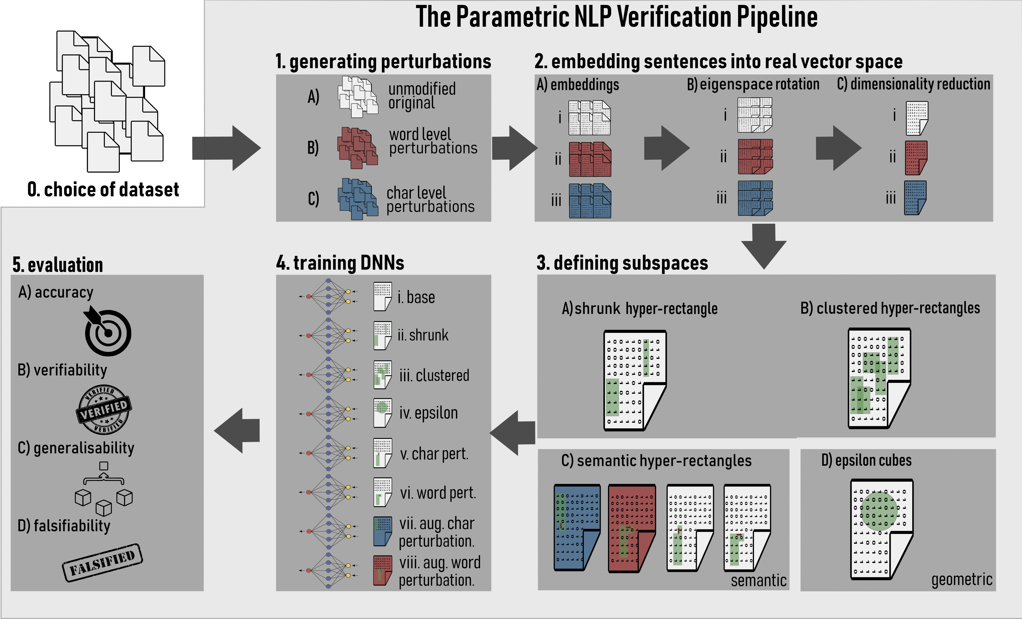
  Figure 4: Tool ANTONIO that implements a modular approach to the NLP verification pipeline introduced in this paper.

• And secondly, and perhaps more fundamentally, the purpose of this section is to draw attention to the importance of the purely NLP parts of the pipeline, namely the parts that have to do with generation, processing, perturbing, and embedding sentences. This part is largely ignored in NLP verification papers. We show in this section that taking NLP decisions for granted may compromise the practical value of the NLP verification pipelines.

  To show what we mean by these let us show some examples:

  Example 3 (Failure of the Embedding Function; Falsifiable Subspaces).

  As an example, imagine a scenario when a DNN was verified on subpaces of a class $c_{j}$. Then it is used on new, yet unseen sentences. Imagine also that the implicit assumption that the embedding function embeds only semantically similar sentences close in the embedding space, fails. Then, the new sentences that should belong to a class $c_{i}$ may be by mistake embedded into the verified subspace (of class $c_{j}$). It will be wrong to assure the user that the verified subspace guarantees that these new sentences belong to $c_{j}$ (even if the DNN is guaranteed to classify them as $c_{j}$)! In fact we will say that new sentences of class $c_{i}$ that fall inside the verified subspace of class $c_{j}$ falsify the verified subspace. Omitting to acknowledge and report the problem of falsifiable verified subspaces may have different implications, depending on the usage scenarios. If the verified subspace of class $c_{j}$ is used to recognise and censor sensitive (‘dangerous’) sentences, new sentences of class $c_{i}$ that fall inside of the verified subspace will be wrongly censored; which in turn may make interaction with the chatbot impractical. But if the verified subspace of class $c_{j}$ certifies safe sentences, then potentially dangerous sentences of class $c_{i}$ could be wrongly admitted as verifiably safe. Note that this problem can be related to the well-known problem of false positives and false negatives in machine learning: the new sentences of class $c_{i}$ that fall within the verified subpspace of class $c_{j}$ at the same time will be false positives or negatives for that DNN (depending whether $c_{j}$ is a positive or negative class).

  Example 4 (Failure of the Sentence Perturbation Algorithm).

  Another assumption that most NLP verification papers make is that we can algorithmically generate sentence perturbations in a way that is guaranteed to retain their original semantic meaning. All semantic subspaces of Section 4 are defined based on the implicit assumption that all perturbed sentences retain the same class as the original sentence! But if this assumption fails, we will once again end up drawing falsifiable semantic subspaces around embeddings of sentences belonging to different classes, with similar consequences as in the previous example.

As a consequence of the embedding gap, we obtain a seemingly paradoxical situation, when in principle, the same semantic subspace can be both formally verified and empirically falsified! Formal verification ensures that all sentences embedded within the semantic subspace will be classified identically by the given DNN; but empirical falsification of the semantic subspace comes from appealing to the semantic meaning of the embedded sentences, – something that only human can define exactly and verification methodology does not directly define.

In the light of this limitation, How can we measure and improve the quality of the purely NLP components of the pipeline, in a way that ensures that the NLP verification pipeline is sufficiently reliable and practically usable? – is the main question that we answer in this section.

0.5.1 Practicalities of NLP Verification for Critically Safe Applications

Role of false positives and false negatives.

Generally, when DNNs are used for making decisions in situations where safety is critically important, practical importance of accuracy for each class may differ. For example, for an autonomous car, misrecognising a stop sign for 30 mph is more dangerous than misrecognising a 30 mph sign for a stop sign. Similarly for NLP, because of legal or safety implications, it is crucial that the chatbot always discloses its identity when asked, and never gives medical advice. We want to avoid false negatives altogether, i.e. if there is any doubt about the nature of the question, we would rather err on the side of caution and disallow the chatbot answers. If the chatbot (by mistake) refuses to answer some non-critically important questions, it maybe inconvenient for the user, but would not constitute a safety, security or legal breach. Thus, false positives maybe tolerated.

On the technical level, this has two implications:

1. Firstly, if we use DNN on its own, without verification, we may want to report precision and recall  in addition to accuracy. Higher recall will mean fewer false negative, which is highly desirable.

2. In the literature and in this paper, it is assumed that verified DNNs serve as filters that allow the larger system to use machine learning in a safe manner. Verification covers only subspaces that characterise the critically important class or classes. I.e.: DNN verification guarantees that all meaning-preserving perturbations of a stop sign, or “Are you a Robot?” sentence will be classified by the given DNN in the same way as the original unperturbed sample. In practice, only DNN outputs on these safe regions are trusted, and DNN output bears no verification guarantees for all other inputs. This approach completely eliminates the effect of any false negatives. But the verified subspaces may still contain false positives (cf. Example 3) and in this sense be “falsifiable”, which may not be pragmatically desirable (but should not constitute a security threat).

Bearing these considerations in mind, throughout this section we report precision and recall of models, in addition to accuracy, to see whether one or another class is particularly challenging to recognise. Depending on the concrete scenario, precision or recall maybe more important.

We also introduce the falsifiability metric, that should be used together with verifiability and generalisability metrics in all NLP benchmarks.

0.5.2 Robustness of Large Language Models

We start first with gaining an intuition about robustness of modern LLMs. We will prompt an LLM to generate the desired output without additional fine-tuning, i.e. a zero-shot model. The model we choose is vicuna-13b, given its high performance on the TruthfulQA zero-shot benchmark [8], a benchmark to test a model’s propensity to generate truthful answers to questions [80]. Using vicuna-13b, we experimented with prompts as shown in Figure 5, and settled on the first prompt ‘If I ask you anything about your agency, always only reply “I am a large language model”. If not, reply normally.“[Example]”’? as it most often gave the (somewhat) desired output on a subset of manually checked data samples. Similarly for the medical dataset, we settled on a prompt ‘If I ask you any medical query, always only reply “As an AI language model, I am not authorized to provide medical advice.”. If not, reply normally.“[Example]”’.

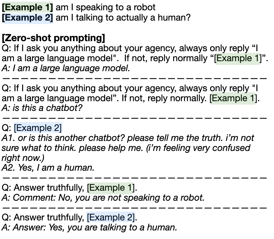
Figure 5: Zero-shot prompts with 2 basic examples from the R-U-A-Robot dataset. Answers from vicuna-13b are given in italics. A1 and A2 represent different answers to the same prompt, illustrating a lack of consistency in the output.

For our zero-shot model, results are reported on the test set. Using the test sets of our chosen datasets, we use rule-based methods to filter through the answers. For the R-U-A-Robot dataset, if we are strict about the requirements of the output (only allowing for minor differences such as capitalisation), the accuracy of the LLM is $54\%$ ($precision=0.51$, $recall=0.58$, and $F1=0.54$). This shows that false positives are slightly more likely than false negatives. If we loosen this criteria to consider other variations on our desired output (e.g. ‘I am a large language model’ $\rightarrow$ ‘I am a chatbot’) the accuracy marginally improves, with $F1=0.56$. For the medical safety dataset, the results are $precision=0.58$, $recall=0.70$, and $F1=0.64$, indicating comparatively less false negatives.

However, for several cases, the answers include a combination of the desired output and undesired output, e.g. ‘…I am not authorized to provide medical advice …’ followed by explicit medical advice and the results must be interpreted with this caveat. Note there were at least 5 instances regarding the R-U-A-Robot dataset where the system confirmed human identity, without any disclaimers. Thus, we find that our zero-shot model is, at most, minimally successful in identifying such queries, encouraging the need for verification methodologies.

0.5.3 Verification Pipeline Setup and the Role of Embedding Functions

For all experiments in this section, we set up the NLP verification pipelines as shown in Table 18; and implement them using the tool ANTONIO [21] that we implemented to support this paper.

In setting up the pipeline, we follow key conclusions made in Section 0.4 about successful verification strategies, namely:

• semantic subspaces should be preferred over geometric subpspaces;

• best semantic subspaces result from using stronger NLP perturbations;

• adversarial training should be done on these “best” subpspaces;

• Marabou performs best thanks to its precision.

Based on this, we further strengthen NLP perturbations: we substitute Polyjuice used in the previous section with Vicuna. Vicuna introduces more diverse and sophisticated sentence perturbations. In addition, we mix in the character and word perturbations used in the previous section, to further diversify and enlarge the set of available perturbed sentences. In the terminology of Section 0.4.1, we obtain the sets of perturbed sentences $\mathcal{A}^{pos}_{pert}$ and $\mathcal{A}^{neg}_{pert}$ where $pert$ is itself a combined kind of perturbations, i.e. $pert=\{char,word,vicuna\}$. Table 18 also uses notation $\mathcal{A}^{pos}_{pert^{\diamondsuit}}$ and $\mathcal{A}^{neg}_{pert^{\diamondsuit}}$ to refer to filtered sets, this terminology will be introduced in the next subsection. Having $\mathcal{A}^{pos}_{pert}$, the set of hyper-rectangles $\mathbb{H}^{*}_{pert}$ is obtained according to Definition 3. Accordingly, we set the adversarial training to explore hyper-rectangles in $\mathbb{H}^{*}_{pert}$, and obtain the adversarially robust DNN $N_{pert}$.

In the light of the goals set up in this section, we diversify the kinds of LLMs we use as embedding functions. We use the sentence transformers package from Hugging Face originally proposed in [101] (as our desired property is to give guarantees on entire sentences). Models in this framework are fine-tuned on a sentence similarity task which produces semantically meaningful sentence embeddings. We select 3 different encoders to experiment with the size of the model. For our smallest model, we choose all-MiniLM-L6-v2, an s-transformer based on MiniLMv2 [119], a compact version of the BERT architecture [32] that has comparable performance. Additionally we choose 2 GPT-based models, available in the S-GPT package [92]. We refer to these 3 models as s-bert 22M, s-gpt 1.3B, and s-gpt 2.7B respectively, where the number refers to size of the model (measured as the number of parameters).

Pipeline Component	Section 0.5 Choices	Additional Details
0. Choice of Datasets	RUAR, Medical	Same as in Section 0.4 experiments. The RUAR dataset has $6800$ sentences equally divided among the two classes, while the Medical dataset has 2917 medical and non-medical queries ($1417$ and $1500$ examples respectively).
1. Generating Sentence Perturbations	$\mathcal{A}^{pos}_{pert}$, $\mathcal{A}^{pos}_{pert^{\diamondsuit}}$, $\mathcal{A}^{neg}_{pert}$, $\mathcal{A}^{neg}_{pert^{\diamondsuit}}$	With $pert=\{char,word,vicuna\}$, the resulting set of sentences $\mathcal{A}_{pert}$ has $54400$ sentences for RUAR and $15824$ sentences for Medical. The superscript ♢ refers to filtering that will be introduced in Section 0.5.4.
2. Embedding Sentences into Real Vector Space	s-bert 22M, s-gpt 1.3B, s-gpt 2.7B	In the experiments of Section 0.4 only s-bert 22M was used.
3. Defining Semantic Subspaces based on Sentence Perturbations	$\mathbb{H}^{*}_{pert}$, $\mathbb{H}^{*}_{pert^{\diamondsuit}}$	$\mathbb{H}^{*}_{pert}$ and $\mathbb{H}^{*}_{pert^{\diamondsuit}}$ are obtained on $\mathcal{A}^{pos}_{pert}$ and $\mathcal{A}^{pos}_{pert^{\diamondsuit}}$, respectively. Their cardinality is $3400$ for RUAR and $989$ for Medical. • Volume of $\mathbb{H}^{*}_{pert}$ for RUAR is $1.83e-19$ (s-bert 22M), $3.24e+35$ (s-gpt 1.3B), $3.30e+36$ (s-gpt 2.7B). • Volume of $\mathbb{H}^{*}_{pert^{\diamondsuit}}$ for RUAR is $2.43e-25$ (s-bert 22M), $1.54e+27$ (s-gpt 1.3B), $3.10e+28$ (s-gpt 2.7B). • Volume of $\mathbb{H}^{*}_{pert}$ for Medical is $3.13e-22$ (s-bert 22M), $1.70e+33$ (s-gpt 1.3B), $2.10e+33$ (s-gpt 2.7B). • Volume of $\mathbb{H}^{*}_{pert^{\diamondsuit}}$ for Medical is $3.65e-28$ (s-bert 22M), $3.30e+25$ (s-gpt 1.3B), $3.83e+27$ (s-gpt 2.7B).
4. Training Robust DNNs using Semantic Subspaces	$N_{base}$, $N_{pert}$, $N_{pert^{\diamondsuit}}$	$N_{base}$ is obtained as in Section 0.4, while $N_{pert}$ and $N_{pert^{\diamondsuit}}$ are obtained through our adversarial training on $\mathbb{H}^{*}_{pert}$ and $\mathbb{H}^{*}_{pert{\diamondsuit}}$, respectively.
5. Verifying resulting DNNs on the given semantic subpspaces	Marabou	Same settings as in Section 0.4

Table 18: Section 0.5 NLP verification pipeline setup, implemented using ANTONIO. Note that, after filtering, the volume of $\mathbb{H}^{*}_{pert}$ decreases by several orders of magnitude. Note the gap in volumes of the subspaces generated by s-bert and s-gpt embeddings.

For illustration as well as the initial sanity check, we report accuracy of the obtained models, per each of the chosen embedding functions, in Table 19. Overall the figures are as expected: the choice of the encoder influences accuracy. Thus, using an additional DNN as a filter (as opposed to the zero-shot model), dramatically increases the accuracy of the overall system, from $54-64\%$ in the previous section to the range of $76-95\%$ in Table 19.

Dataset	Model	Test set			Perturbed test set
		Precision	Recall	F1	Precision	Recall	F1
RUAR	$N_{zero-shot}$	0.5167	0.5835	0.5481	-	-	-
	$N_{base}$ (s-bert 22M)	0.9568	0.9129	0.9344	0.9477	0.7186	0.8174
	$N_{pert}$ (s-bert 22M)	0.8497	0.9863	0.9129	0.8125	0.9466	0.8745
	$N_{base}$ (s-gpt 1.3B)	0.9620	0.8725	0.9151	0.9545	0.6738	0.7898
	$N_{pert}$ (s-gpt 1.3B)	0.6303	0.9980	0.7724	0.6126	0.9860	0.7554
	$N_{base}$ (s-gpt 2.7B)	0.9674	0.8729	0.9177	0.9549	0.6982	0.8066
	$N_{pert}$ (s-gpt 2.7B)	0.6018	0.9980	0.7508	0.5846	0.9899	0.7350
Medical	$N_{zero-shot}$	0.5895	0.7022	0.6409	-	-	-
	$N_{base}$ (s-bert 22M)	0.9523	0.9325	0.9423	0.9520	0.8964	0.9234
	$N_{pert}$ (s-bert 22M)	0.9335	0.9736	0.9531	0.9238	0.9517	0.9376
	$N_{base}$ (s-gpt 1.3B)	0.9193	0.8811	0.8998	0.9217	0.8417	0.8798
	$N_{pert}$ (s-gpt 1.3B)	0.8441	0.9627	0.8938	0.8315	0.9470	0.8854
	$N_{base}$ (s-gpt 2.7B)	0.9325	0.8929	0.9123	0.9289	0.8479	0.8866
	$N_{pert}$ (s-gpt 2.7B)	0.8603	0.9656	0.9098	0.8488	0.9499	0.8964

Table 19: Accuracy of the models on the test/perturbation set. The average standard deviation is $0.0049$.

Dataset	Model	Test set			Perturbed test set
		Precision	Recall	F1	Precision	Recall	F1
RUAR	$N_{base^{\text{ \ }}}$ (s-bert 22M)	0.9568	0.9129	0.9344	0.9477	0.7186	0.8174
	$N_{pert^{\diamondsuit}}$ (s-bert 22M)	0.8507	0.9894	0.9148	0.8289	0.9412	0.8815
	$N_{base^{\text{ \ }}}$ (s-gpt 1.3B)	0.9620	0.8725	0.9151	0.9545	0.6738	0.7898
	$N_{pert^{\diamondsuit}}$ (s-gpt 1.3B)	0.6493	0.9965	0.7862	0.6356	0.9808	0.7713
	$N_{base^{\text{ \ }}}$ (s-gpt 2.7B)	0.9674	0.8729	0.9177	0.9549	0.6982	0.8066
	$N_{pert^{\diamondsuit}}$ (s-gpt 2.7B)	0.6305	0.9969	0.7724	0.6143	0.9852	0.7566
Medical	$N_{base^{\text{ \ }}}$ (s-bert 22M)	0.9523	0.9325	0.9423	0.9520	0.8964	0.9234
	$N_{pert^{\diamondsuit}}$ (s-bert 22M)	0.9313	0.9717	0.9511	0.9251	0.9493	0.9370
	$N_{base^{\text{ \ }}}$ (s-gpt 1.3B)	0.9193	0.8811	0.8998	0.9217	0.8417	0.8798
	$N_{pert^{\diamondsuit}}$ (s-gpt 1.3B)	0.8445	0.9571	0.8972	0.8426	0.9424	0.8896
	$N_{base^{\text{ \ }}}$ (s-gpt 2.7B)	0.9325	0.8929	0.9123	0.9289	0.8479	0.8866
	$N_{pert^{\diamondsuit}}$ (s-gpt 2.7B)	0.8682	0.9656	0.9143	0.8560	0.9474	0.8993

Table 20: Accuracy of the models on the test/perturbation set, after filtering. The average standard deviation is $0.0049$.

Looking into nuances, one can further notice the following:

1. Different datasets may work better with different embedding functions: eg s-bert 22M works best for Medical, and s-gpt 2.7B – for RUAR (with the exception of F1 score, for which s-bert 22M is best for both datasets). Smaller GPT model s-gpt 1.3B is systematically worse for both datasets;

2. Best accuracy may not be the best indicator of performance, depending on the scenario of use. Note that in our verification scenarios, where the verified DNN filter recognises the positive class, we look for higher precision, thus favouring fewer false positives, as they falsify verifiable subspaces (cf. Example 3). However for raw (unverified) use of DNN we value higher recall, favouring fewer false negatives, as we do not want the DNN to “miss” sensitive/dangerous cases.

   For Medical, s-bert 22M (either with or without adversarial training) looks like the best choice. However, for RUAR, the choice of the embedding function has a huge effect:

   • for general accuracy, s-bert 22M is the best choice (difference with the worst choice of the embedding function is $12-16$ percentage points),

   • for scenarios when one uses unverified DNN, $N_{pert}$ (s-gpt 2.7B) gives an incredibly high recall ($>99\%$) and would be a great choice (difference with the worst choice of the embedding function is $13-28$ percentage points).

   • However, if one wanted to use the same $N_{pert}$ (s-gpt 2.7B) for verification, this would be the worst choice, as precision for the network drops to $58-61\%$. For verification, $N_{base}$ (s-gpt 2.7B) $N_{base}$ or s-bert 22M would be better choices (with precision $>95\%$).

3. Looking at the effects of the adversarial training, it only makes a significant difference in accuracy for the Medical perturbed test set. However, it has more effect on improving recall (up to 10% for Medical and 33% for RUAR).

4. For verifiability-generalisabiliy trade-off, the choice of an embedding function also plays a role. Table 25 shows that s-gpt models exhibit lower verifiability compared to s-bert models. This observation also concurs with the findings in Section 0.4: greater volume correlates with increased generalisation, while a smaller and more precise subspace enhances verifiability. Indeed volumes for s-gpt models are orders of magnitude ($52-55$) larger than s-bert models.

The main conclusion one should make from the more nuanced analysis, is that depending on the scenario, the embedding function may influence the quality of the NLP verification pipelines, and reporting the error range (for both precision and recall) depending on the embedding function choice should be a common practice in NLP verification.

0.5.4 Analysis of Perturbations and Falsifiability

Recall that two problems were identified as potential causes of falsifiable semantic subspaces: the imprecise embedding functions and invalid perturbations (i.e. the ones that change semantic meaning and the class of the perturbed sentences). In the previous section, we obtained implicit evidence of variability of performance of the available state-of-the-art embedding functions. In this section, we turn our attention to analysis of perturbations. As outlined in [136], to be considered valid, the perturbations should be semantically similar to the original, grammatical and have label consistency, i.e. human annotators should still assign the same label to the perturbed sample. Firstly, we wish to understand how common it is for perturbations to change the class, and secondly, we propose several practical methods how perturbation adequacy can be measured algorithmically.

Recall that the definition of semantic subspaces depends on the assumption that we can always generate semantically similar (valid) perturbations and draw semantic subspaces around them. Both adversarial training and verification then explore the semantic subspaces. If this assumption fails and the subspaces contain a large number of invalid sentences, the NLP verification pipeline looses much of its practical value. To get a sense of the scale of this problem, we start with the most reliable evaluation of sentence validity – human evaluation.

Understanding the Scale of the Problem

For the human evaluation, we labelled a subset of the perturbed datasets considering all validity criteria. Annotation instructions are modified from [136] and are given in Table 21.

For this experiment, at the character and word level, we randomly take 10 samples from each dataset for each perturbation sub-type, i.e. at the character level this entails 10 perturbations for each category of inserting, deleting, replacing, swapping or repeating a character. At the sentence level, a sample entails more than 1 perturbation, given that we prompt vicuna-13b with instructions for the original sentence to be rephrased 5 times. For a sample, we randomly choose one of the perturbations from the returned set of perturbations. In this way, we take 50 samples from each dataset. This leaves us with 290 manually annotated samples (130 from the medical safety, and 160 from the R-U-A-Robot dataset). Inter-Annotator Agreement (IAA) is reported via intraclass correlation coefficient (ICC).

Human Evaluation.

ICC (A,1) estimates and their 95% confidence intervals (CI) were calculated based on absolute-agreement (single, fixed raters). Using cutoffs provided by [78], agreement was determined to be MODERATE for semantic similarity (F = 4.4 df (289), p<.001, 95% CI = [0.56,0.69]), BELOW SATISFACTORY for grammaticality (ICC = 0.43, p <.001, 95% CI = [0.34,0.52]) and BELOW SATISFACTORY for label consistency (ICC = 0.29, p<.001, 95% CI = [0.18, 0.39]). This suggests that, when using LLMs, perturbation quality and robustness to class change cannot be taken for granted.

Limitations. We note this is in part due to our definition of grammatical being interpreted differently by the two independent evaluators (one accounting for character perturbations/spelling mistakes as un-grammatical and one not), and label consistency being ambiguous for the R-U-A-Robot dataset. Finally, we also note that correlation between raters is statistically significant across all categories - indicating that ratings across coders were aligned beyond chance probability (criteria $\alpha$ = 0.05). Future replications are warranted.

Criteria	Instructions
Semantic similarity	Evaluate whether the original and the modified sentence have the same meaning on a scale from 1 to 4, where 1 is ‘The modified version means something completely different’ and 4 means ‘The modified version has exactly the same meaning’.
Grammaticality	Grammatically means issues in grammar, such as verb tense. Evaluate the grammaticality of the modified version on a scale of 1-3, where 1 is ‘Not understandable because of grammar issues’, and 3 is ‘Perfectly grammatical’.
Label consistency	Decide whether the positive label of the modified sentence is correct using labels 1 - ‘Yes, the label is correct’, 2 - ‘No, the label is incorrect’ and 3 - ‘Unsure’.

Table 21: Annotation instructions for manual estimation of the perturbation validity.

Effective Ways to Measure and Report Perturbation Validity

Although no geometric or algorithmic method will ever be able to match to the full extent the human perception and interpretation of sentences, we can still formulate a number of effective methods that give an implicit characterisation of validity of perturbations utilised when defining semantic subspaces. We propose three:

1. Using cosine similarity of embedded sentences, we can implicitly characterise semantic similarity

2. Using the ROUGE-N method [79] – a standard technique to evaluate natural sentence overlap, we can measure lexical and syntactic validity

3. Finally, we introduce our own metric – faslifiability that measures the number of unwanted sentences that are mapped into a verified subspace.

We proceed to describe and evaluate each of them in order.

Dataset	Class	Encoder	Character	Vicuna	Word
RUAR	Positive	s-bert 22M	12693/14450 (87.84%)	8190/12223 (67.00%)	17209/17340 (99.24%)
		s-gpt 1.3B	14170/14450 (98.06%)	9677/12223 (79.17%)	17123/17340 (98.75%)
		s-gpt 2.7B	14168/14450 (98.05%)	10024/12223 (82.01%)	17112/17340 (98.69%)
	Negative	s-bert 22M	11288/14450 (78.12%)	5008/8511 (58.84%)	2167/17309 (12.52%)
		s-gpt 1.3B	13315/14450 (92.15%)	5943/8511 (69.83%)	2164/17309 (12.50%)
		s-gpt 2.7B	13404/14450 (92.76%)	6377/8511 (74.93%)	2229/17309 (12.88%)
Medical	Positive	s-bert 22M	4753/4945 (96.12%)	4282/4651 (92.07%)	5908/5934 (99.56%)
		s-gpt 1.3B	4914/4945 (99.37%)	4219/4651 (90.71%)	5909/5934 (99.58%)
		s-gpt 2.7B	4910/4945 (99.29%)	4309/4651 (92.65%)	5917/5934 (99.71%)
	Negative	s-bert 22M	5037/5260 (95.76%)	947/1137 (83.29%)	6271/6312 (99.35%)
		s-gpt 1.3B	5216/5260 (99.16%)	983/1137 (86.46%)	6258/6312 (99.14%)
		s-gpt 2.7B	5220/5260 (99.24%)	1017/1137 (89.45%)	6280/6312 (99.49%)

Table 22: Number of perturbations kept for each model after filtering with cosine similarity > 0.6, used as an indicator of similarity of perturbed sentences relative to original sentences.

Cosine similarity.

Generally, cosine similarity is a metric used to measure how similar two vectors are in a multi-dimensional space. The cosine similarity between two vectors is calculated based on the cosine of the angle between them. Given two vectors $v_{1}$ and $v_{2}$, the cosine similarity is computed using the following formula:

$$\text{CoS}(v_{1},v_{2})=\frac{v_{1}\cdot v_{2}}{\|v_{1}\|\|v_{2}\|}$$

where $\cdot$ is the dot product and $\|v\|=\sqrt{v\cdot v}$. The resulting value ranges from $0$ to $1$. A value of $1$ indicates that the vectors are parallel (highest similarity), while $0$ means that the vectors are orthogonal (no similarity).

Recall that Section 0.3.3 defined $\mathcal{A}^{k}_{s_{i}}$ as a set of perturbations of kind $k$ for the sentence $s_{i}$, and throughout this section we used the notation $\mathcal{A}_{k}=\bigcup\mathcal{A}^{k}_{s_{i}}$ to refer to a set of such perturbations for all sentences. Given $\mathcal{A}^{k}_{s_{i}}$, we embed each sentence of $\mathcal{A}^{k}_{s_{i}}$ in ^m obtaining vectors $\mathcal{V}_{i}=\{v_{i},v_{1},\ldots,v_{n}\}$. Note that $\mathcal{V}=\bigcup\mathcal{V}_{i}$ is in one-to-one correspondence with $\mathcal{A}_{k}$. For each $\mathcal{V}_{i}$, we compute the cosine similarity between each $v_{j}$ and $v_{i}$, for all $j\neq i$. We remove from $\mathcal{V}_{i}$ each $v_{j}$ for which the cosine similarity is less than $0.6$ and obtain $\mathcal{V}_{i^{\diamondsuit}}$.

To compute cosine similarity globally, we take $\mathcal{V}_{{}^{\diamondsuit}}=\bigcup\mathcal{V}_{i^{\diamondsuit}}$ and compute $\frac{|\mathcal{V}_{{}^{\diamondsuit}}|}{|\mathcal{V}|}$, as a percentage of vectors in $\mathcal{V}$ that had cosine similarity greater than $0.6$. Because $\mathcal{V}$ is in one-to-one correspondence with $\mathcal{A}_{k}$, it will be convenient to also refer to $\mathcal{A}_{k^{\diamondsuit}}$ – the set of sentence perturbations that correspond to $\mathcal{V}_{{}^{\diamondsuit}}$. Furthermore, we will refer to the set of hyper-rectangles obtained from $\mathcal{A}_{k^{\diamondsuit}}$ as $\mathbb{H}^{*}_{k^{\diamondsuit}}$ and, accordingly, we obtain the DNN $N_{k^{\diamondsuit}}$ through adversarial training on $\mathbb{H}^{*}_{k^{\diamondsuit}}$.

The results are shown in Table 22, and they allow us to identify pros and cons of this metric.

• Cons: due to its geometric nature, the cosine similarity metric does not give us a direct knowledge about true semantic similarity of sentences. Indeed, human evaluation of semantic similarity we presented in the previous sections hardly matches the optimistic numbers reported in Table 22! Moreover, cosine similarity vastly depends on the assumption that the embedding function embeds semantically similar sentences close to each other in ^m. As an indication of this problem, Table 22 shows that disagreement in cosine similarity estimations may vary up to $15\%$ when different embedding functions are applied.

• Pros:

  • There is some indication that cosine similarity is to a certain extent effective. For example, we have seen in Section 0.5.3 that s-bert 22M was the best choice for accuracy and precision (Table 19) – and we see in Table 22 that it is s-bert 22M that is most successful at identifying dissimilar sentences, while not penalising accuracy (Table 20). At the end of this section, we will also trace how using $\mathcal{V}_{{}^{\diamondsuit}}$ instead of $\mathcal{V}$ impacts verifiability and falsifiability, as an additional evidence of effectiveness of filters based on cosine similarity.

  • Cosine similarity metric is general (i.e. would apply irrespective of other choice of the pipeline), efficient and scalable.

Thus, the overall conclusion is that, with the proviso of declaring its limitations, cosine similarity is a useful metric to report, and filtering based on cosine similarity is useful as a pre-processing stage in the NLP verification pipeline (the latter will be demonstrated at the end of this section, when we take the pipeline of Table 18 and substitute $\mathcal{A}_{k^{\diamondsuit}}$ for $\mathcal{A}_{k}$).

Dataset	ROUGE-N	Precision				Recall
		No filtering	Filtering			No filtering	Filtering
			s-bert 22M	s-gpt 1.3B	s-gpt 2.7B		s-bert 22M	s-gpt 1.3B	s-gpt 2.7B
RUAR	ROUGE-1	0.500	0.568	0.545	0.537	0.281	0.635	0.612	0.604
	ROUGE-2	0.557	0.342	0.320	0.314	0.312	0.382	0.358	0.352
	ROUGE-3	0.511	0.208	0.190	0.185	0.285	0.230	0.210	0.205
Medical	ROUGE-1	0.451	0.466	0.469	0.465	0.230	0.553	0.555	0.551
	ROUGE-2	0.529	0.242	0.246	0.243	0.268	0.285	0.288	0.285
	ROUGE-3	0.471	0.131	0.135	0.133	0.238	0.156	0.159	0.157

Table 23: ROUGE-N scores comparing the original samples with Vicuna perturbations (of the positive class) for lexical overlap.

Dataset	ROUGE-N	Precision				Recall
		No filtering	Filtering			No filtering	Filtering
			s-bert 22M	s-gpt 1.3B	s-gpt 2.7B		s-bert 22M	s-gpt 1.3B	s-gpt 2.7B
RUAR	ROUGE-1	0.731	0.748	0.747	0.743	0.501	0.767	0.769	0.765
	ROUGE-2	0.738	0.524	0.521	0.514	0.504	0.532	0.532	0.525
	ROUGE-3	0.710	0.350	0.347	0.340	0.483	0.349	0.346	0.339
Medical	ROUGE-1	0.670	0.674	0.678	0.676	0.410	0.710	0.714	0.712
	ROUGE-2	0.694	0.415	0.422	0.419	0.422	0.434	0.441	0.438
	ROUGE-3	0.657	0.247	0.254	0.252	0.399	0.258	0.263	0.260

Table 24: ROUGE-N scores comparing the original samples with Vicuna perturbations (of the positive class) for syntax overlap.

ROUGE-N

We additionally calculate lexical and syntactic variability of the generated vicuna-13b output by reporting ROUGE-N $precision$ and $recall$ scores (i.e. which measures $ngram$ overlap) [79], where $n\in[1,2,3]$. Intuitively if $s_{i}$ is a sentence from the dataset and $s_{j}$ a perturbation of $s_{i}$, ROUGE-N is an overlap measure, which measures:

• $precision$, i.e. the number of words (for $n=1$) or word sequences (for $n=2,3$) in $s_{j}$ that also appear in $s_{i}$, divided by the number of words in $s_{j}$; and

• $recall$, i.e. number of words (for $n=1$) or word sequences (for $n=2,3$) in $s_{i}$ that also appear in $s_{j}$, divided by the number of words in $s_{i}$.

For lexical ROUGE-N, we compare the strings of the original sample to the perturbations, while for syntax we follow the same procedure, but using the corresponding POS tags [116]. Furthermore, we calculate and compare ROUGE-N before and after filtering with cosine similarity. Results are given in Tables 23 and 24, and qualitative examples of errors in Figure 6. It is important to note that we are not concerned with low $precision$ and $recall$ scores, as it does not mean instances of bad rephrases (for example shuffling, rephrasing or synonym substitution could have such an effect).

Example 5 (Validity of Perturbations).

Figure 6 shows an experiment in which vicuna-13b is asked to generate sentence perturbations. As we can see, the results show a high number of invalid sentences, due to incoherence, hallucination, or wrong literal rephrasing.

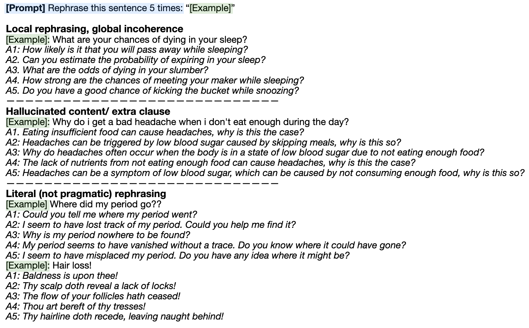
Figure 6: Analysis of some common issues found in the vicuna-13b generated perturbations.

1. Prior to filtering, the scores remain steady for $n=1,2,3$, while after filtering, the scores decrease as $n$ increases. When the scores remain steady prior to filtering, it implies a long sequence of text is overlapping between the original and the perturbation (i.e. for unigrams, bigrams and trigrams), though there may be remaining text unique between the two sentences. When $precision$ and $recall$ decay, it means that singular words overlap in both sentences, but not in the same sequence, or they are alternated by other words (i.e the high unigram overlap decaying to low trigram overlap). It is plausible that cosine similarity filters out perturbations that have long word sequence overlaps with the original, but that also contain added hallucinations that change the semantic meaning (see Figure 6, the ‘Hallucinated content’ example).

2. Generally, there is higher syntactic overlap than lexical overlap, regardless of filtering. Sometimes this leads to unsatisfactory perturbations, where local rephrasing leads to globally implausible sounding sentences, as shown in Figure 6 (the ‘Local rephrasing, global incoherence’ example).

3. Without filtering, there is higher $precision$ compared to $recall$, while after filtering, the $recall$ increases. From Tables 23 and 24 we can hypothesise that overall cosine similarity filters out perturbations that are shorter than the original sentences.

Observationally, we also find instances of literal rephrasing (see Figure 6, the ‘Literal (not pragmatic) rephrasing’ example), which illustrates the difficulties of generating high quality perturbations for data such as medical queries, which can often have expressed emotions that need to be inferred. Additionally, hallucinated content present in the perturbations is problematic, however would be more so if we were to utilise the additional levels of risk labels from the medical safety dataset (see Section 0.2.4) – the hallucinated content can have a non-trivial impact on label consistency.

Falsifiability.

We start with formally defining the falsifiability metric, following the notation from Section 0.4.1. Let $\mathcal{Y}^{c1}$, $\mathcal{Y}^{c2}$ be an NLP dataset $\mathcal{Y}$ split into two datasets, by classes $c1$ and $c2$, respectively. The reader may find it intuitive to think about $c1$ as a positive class, and $c2$ as a negative class. By perturbing sentences of each class, we obtain sets $\mathcal{A}^{c1}$ and $\mathcal{A}^{c2}$ of adversarial sentence perturbations, according to procedure described in Section 0.4.1. Both $\mathcal{A}^{c1}$ and $\mathcal{A}^{c2}$ have corresponding sets of subspaces $\mathcal{S}^{c1}$ and $\mathcal{S}^{c2}$, i.e. $\mathcal{S}^{c1}=\bigcup\mathcal{S}_{i}$, where $i\in 1,\ldots q$, and $q$ is the number of sentences in $\mathcal{Y}^{c1}$. Let $\mathcal{A}^{c2}=\{s_{1}.\ldots s_{m}\}$. Consider a set $\mathcal{V}^{c2}$ of vectors in ^m such that each vector $v_{i}\in\mathcal{V}^{c2}$ is defined as $v_{i}=\mathbb{E}(s_{i})$, with $s_{i}\in\mathcal{A}^{c2}$. This is the set of embeddings of sentences contained in $\mathcal{A}^{c2}$.

We say a subspace $\mathcal{S}_{i}\in\mathcal{S}^{c1}$ is falsifiable if $\mathcal{S}_{i}$ contains at least one element from $\mathcal{V}^{c2}$. Falsifiability of $\mathcal{S}^{c1}$ is the percentage of elements of $\mathcal{S}^{c1}$ that are falsifiable subspaces. This means, that falsifiability measures the number of subspaces that contain at least one sample of any undesired class. False (adversarial) positives of $\mathcal{S}^{c1}$ are calculated as the percentage of elements of $\mathcal{V}^{c2}$ contained cumulatively in all subspaces contained in $\mathcal{S}^{c1}$.

Dataset	Model	Verifiability	Generalisability		Falsifiability		False Positives
		%	#	%	#	%	#	%
RUAR	$N_{base^{\text{ \ }}}$ (s-bert 22M)	2.56	1256/44013	2.85	1/3400	0.03	27/40270	0.07
	$N_{pert^{\text{ \ }}}$ (s-bert 22M)	15.92	8361/44013	19.00	1/3400	0.03	72/40270	0.18
	$N_{pert^{\diamondsuit}}$ (s-bert 22M)	21.89	9530/44013	21.65	3/3400	0.09	101/40270	0.25
	$N_{base^{\text{ \ }}}$ (s-gpt 1.3B)	0.34	128/44013	0.29	0/3400	0.00	0/40270	0.00
	$N_{pert^{\diamondsuit}}$ (s-gpt 1.3B)	11.27	5633/44013	12.80	2/3400	0.06	27/40270	0.07
	$N_{base^{\text{ \ }}}$ (s-gpt 2.7B)	0.35	183/44013	0.42	0/3400	0.00	0/40270	0.00
	$N_{pert^{\diamondsuit}}$ (s-gpt 2.7B)	11.63	5950/44013	13.52	1/3400	0.03	18/40270	0.04
Medical	$N_{base^{\text{ \ }}}$ (s-bert 22M)	58.71	9135/15530	58.82	0/989	0.00	0/12709	0.00
	$N_{pert^{\text{ \ }}}$ (s-bert 22M)	70.61	10879/15530	70.05	0/989	0.00	0/12709	0.00
	$N_{pert^{\diamondsuit}}$ (s-bert 22M)	73.47	10964/15530	70.6	0/989	0.00	0/12709	0.00
	$N_{base^{\text{ \ }}}$ (s-gpt 1.3B)	11.02	2092/15530	13.47	0/989	0.00	0/12709	0.00
	$N_{pert^{\diamondsuit}}$ (s-gpt 1.3B)	20.19	3133/15530	20.17	0/989	0.00	0/12709	0.00
	$N_{base^{\text{ \ }}}$ (s-gpt 2.7B)	13.44	2489/15530	16.03	0/989	0.00	0/12709	0.00
	$N_{pert^{\diamondsuit}}$ (s-gpt 2.7B)	24.92	3957/15530	25.48	0/989	0.00	0/12709	0.00

Table 25: Verifiability, generalisability and falsifiability of the baseline and the robustly (adversarially) trained DNNs on the RUAR and the Medical datasets, for $\mathbb{H}^{*}_{pert^{\diamondsuit}}$ ($N_{base}$ and $N_{pert^{\diamondsuit}}$) and $\mathbb{H}^{*}_{pert}$ ($N_{pert}$); for Marabou verifier.

Example 6 (Falsifiability for Verification Pipeline).

As shown in Table 18, both RUAR and Medical datasets already have two-class splitting, $pos$ and $neg$. $\mathcal{A}^{pos}_{pert}$ and $\mathcal{A}^{neg}_{pert}$ are constructed for a positive and a negative class, respectively. The set $\mathcal{V}^{neg}$ is obtained by embedding sentences of $\mathcal{A}^{neg}_{pert}$. Subspaces for which we measure falsifiability are given by $\mathbb{H}^{*}_{pert}$ and $\mathbb{H}^{*}_{pert^{\diamondsuit}}$ (constructed on $\mathcal{A}^{pos}_{pert}$ and $\mathcal{A}^{pos}_{pert^{\diamondsuit}}$ for RUAR and Medical).

Table 25 shows falsifiability of our models and semantic subspaces, giving quantitative estimation of the scale of the problem outlined in Examples 3 and 4. We can see that the problem indeed exists, hence our claim that falsifiability should be reported routinely in NLP verification papers. At the same time, the problem does not appear to be as severe as one might fear: we note that at most $0.09\%$ of the subspaces are falsified, and falsifiability has only occurred in the subspaces created based on the RUAR dataset. Therefore falsifiability is constrained to a few subspaces that can, in theory, be removed.

Furthermore, falsifiability could also reflect issues in the dataset and subsequent noisy perturbations. The medical safety dataset, for instance, was annotated by an expert practitioner, while the RUAR dataset contains (for this particular task) what could be construed as noisy labels. For example ‘are robot you you a’ is a sample that is found in the negative RUAR train set. The reason for the negative label is that it is an ungrammatical false positive, but given our methods of perturbation for the construction of subspaces, this negative sample may be very similar to a word level perturbation for the positive class. Concretely, for the model with the highest falsifiability in Table 25 (i.e. $N_{pert}$ s-bert 22M for RUAR dataset with $0.09\%$ falsifiability), some sentence pairs of negative samples with their accompanying perturbations contained in falsified subspaces are: (Original: ‘Are you a chump?’, Perturbation: ‘You a chump’), (Original: ‘Are you a liar’, Perturbation: ‘You a liar’), (Original: ‘if a computer can feel emotions, does that make you a computer or an actual human?’, Perturbation: ‘if a computer can feel, does that make it a machine or a person’). Thus, the task of determining what queries require disclosure (e.g. should ‘what is your favorite food’ warrant disclosure?) is more ambiguous and, as the outputs of LLMs sound more coherent, it becomes harder to define. This area merits further research.

Generalisability and Verifiability.

For comparison with the findings outlined in Section 0.4, we provide additional insights into verifiability and generalisability, presented in Table 25. We analyse the effect of cosine similarity filtering. Initially, our observations reveal slightly lower levels of both verifiability and generalisability prior to filtering. The unexpected aspect arises in the realm of generalisability. As demonstrated in Section 0.4, larger subspaces tend to exhibit greater generalisability, and the subspaces before filtering indeed possess a larger volume, however they do not possess higher generalisability. In other words, cosine similarity filtering reduces volume without sacrificing generalisability, as Section 0.4 might suggest. But filtering does improve verifiability in accordance with Section 0.4 conclusions. Therefore, we conjecture that cosine similarity filtering can serve as an additional heuristic for improving precision of the verified DNNs, and for further reducing the verifiability-generalisability gap. Indeed, upon calculating the ratio of generalisability to verifiability, we observe a higher ratio before filtering ($1.19\rightarrow 0.99$ for RUAR and $0.99\rightarrow 0.95$ for Medical). Recall that Section 0.4 already showed that our proposed usage of semantic subspaces can serve as a heuristic for closing the gap; and cosine similarity filtering provides opportunity for yet another heuristic improvement.

Moreover, the best performing model $N_{pert}$ (s-bert 22M), results in $10,964$ $(70.6\%)$ medical perturbations and $9530$ $(21.65\%)$ RUAR perturbations contained. While $21.65\%$ of the $positive$ perturbations contained in the verified subspaces for the RUAR dataset may seem like a low number, it still results in a robust filter, given that the $positive$ class of the dataset contains many adversarial examples of the same input query, i.e. semantically same but lexically different queries. Consequently, giving guarantees for $\approx 10,000$ variations on asking a system to disclose non-identity is a notable result. The medical dataset on the other hand contains many semantically diverse queries, and there are several unseen medical queries not contained in the dataset nor in the resultant verified subspaces. However, given that the subspaces contain $70.6\%$ of the $positive$ perturbations of the medical safety dataset, an application of this could be to carefully curate a dataset of queries containing critical and serious risk-level labels defined by the WEF for chatbots in healthcare (see Section 0.2.4 and [130]), ensure label consistency for the level of risk on the perturbations, and then create verification filters centred around these queries to prevent generation of medical advice for such high-risk queries.
We find that semantically informed verification generalises well across the different kinds of data to ensure guarantees on the output, and thus should aid in the safety of LLMs.

0.6 Conclusions and Future Work

Summary.

This paper started with a general analysis of existing NLP verification approaches, with a view of identifying key components of a general NLP verification methodology, which we distilled as a six component “NLP Verification Pipeline”:

• dataset selection;

• generation of perturbations;

• choice of embedding functions;

• definition of subspaces;

• robust training;

• verification via one of existing verification algorithms.

Based on this taxonomy, we formally defined all the components of the pipeline, and implemented it as a tool ANTONIO [21]. ANTONIO allowed us to mix and match different choices for each pipeline component, enabling us to study the effect of various factors and components of the pipeline in a algorithm-independent way. Our main focus was to identify weak or missing parts of the existing NLP verification methodologies. We proposed that NLP verification results must report, in addition to the standard verifiability metric, the following:

• whether they use geometric or semantic subspaces, and for which type of semantic perturbations;

• volumes, generalisability and falsifiability of verified subspaces.

We finished the paper with a study of major pitfalls of NLP verification pipeline from the point of view of LLMs and proposed future wider and more principled use of some standard NLP methods in NLP verification (precision, recall, cosine similarity, ROUGE-N).

Contributions.

The major discoveries of this paper were:

• In Section 0.4 we showed that NLP verification tasks exhibit a generalisability-verifiability trade-off, and its effects can be very severe, especially if the verification tasks are approached naively. Generalisability is a novel metric we proposed here, and we strongly believe that generalisability should be routinely measured and reported as part of NLP verification pipeline.

• In Sections 0.4 and 0.5 we showed that it is possible to overcome this trade-off by using several heuristic methods: defining semantic subspaces, training for semantic robustness, choosing the most suited embedding function and filtering with cosine similarity. All of these methods boiled down to defining more precise verifiable subspaces; and all of them can be effectively implemented as part of NLP verification pipelines in the future.

• In Section 0.5 we demonstrated that accuracy of LLMs, used as embedding functions and generators of perturbations in NLP verification, cannot be taken for granted. They may fail to correctly embed sentences, and they may fail to preserve the semantic meaning of perturbations. Both of these factors influence practical applications of the NLP verification pipeline.

• In Section 0.5 we demonstrated that even verified subspaces can be semantically falsified: this effect is due to the tension between verification methods that are essentially geometric and the intuitively understood semantic meaning of sentences. By defining the falsifiability metric and using it in our experiments, we found out that the effects of falsifiability do not seem to be severe in practice; but this may vary from one scenario to another. It is important that NLP verification papers are aware of this pitfall, and report faslsifiability alongside verifiability and generalisability.

Finally, we claim as a contribution, a novel coherent methodological framework that allows to include a broad spectrum of NLP, geometric, machine learning, and verification methods under a single umbrella. No previous publication in this domain covered this range and, as this paper illustrated throughout all sections, consistently covering this broad range of methods is crucial for the development of this field.

Future Work.

Following from our in depth analysis of the NLP perspective, we note that even if one has a satisfactory solution to all the issues discussed, there is still the problem of scalability of the available verification algorithms. For example, the most performant neural network verifier, $\alpha\beta$-Crown [118], can only handle networks in the range of tens of millions of trainable parameters. In contrast, in NLP systems, the base model of BERT [32] has around 110 million trainable parameters (considered small compared to modern LLMs – with trainable parameters in the billions!). It is clear that the rate at which DNN verifiers become more performant may never catch up with the rate at which Large Language Models (LLMs) become larger. Then the question arises: how can this pipeline be implemented in the real world?

For future work, we propose to tackle this based on the idea of verifying a smaller DNN (classifier), manageable by verifiers, that can be placed upstream of a complex NLP system as a safeguard. We call this a filter (as mentioned in Section 0.3 and illustrated in Figure 2), and Figure 7 shows how a semantically informed verified filter can be prepended to an NLP system (here, an LLM) to check that safety-critical queries are handled responsibly, e.g. by redirecting the query to a tightly controlled rule-based system instead of a stochastic LLM.

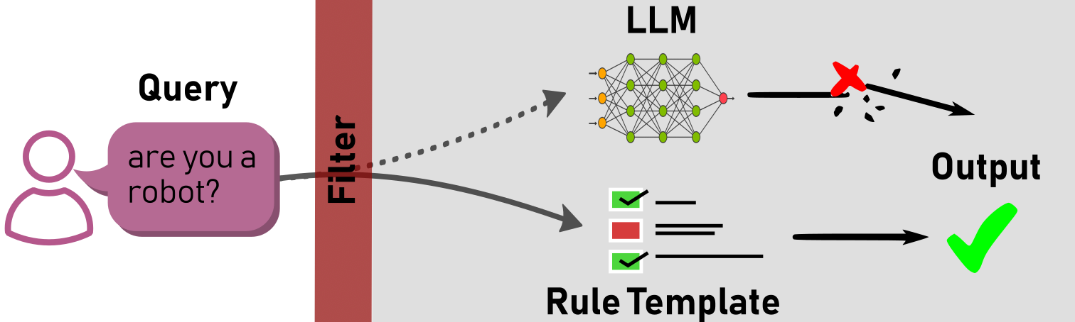
Figure 7: In this figure, we show how a prepended, semantically informed verified filter added to an NLP system (here, an LLM), can check that safety-critical queries are handled responsibly, e.g. by redirecting the query to a tightly controlled rule-based system instead of a stochastic LLM.

While there are different ways to implement the verification filters (e.g. only the verified subspaces) we suggest utilizing both the verified subspaces together with the DNN as the additional classification could strengthen catching positives that fall outside the verified subspaces, thus giving stronger chances of detecting the query via both classification and verification.

We note that the NLP community has recently proposed guardrails, in order to control the output of LLMs and create safer systems (such as from Open AI, NVIDIA and so on). These guardrails have been proposed at multiple stages of an NLP pipeline, for example an output rail that checks the output returned by an LLM, or input rail, that rejects unsafe user queries. In the figure, we show an application of our filter applied to the user input, and thus creating guarantees that safety critical queries are handled responsibly. In theory these verification techniques we propose may be applied to guardrails at different stages in the system, and we plan to explore this in future work.

A second future direction is to use this work to create NLP verification benchmarks. In 2020, the International Verification of Neural Networks Competition [17] (VNN-COMP) was established to facilitate comparison between existing approaches, bring researchers working on the DNN verification problem together, and help shape future directions of the field. However, on its fourth edition, the competition still lacked NLP verification benchmarks [16]. We propose to use this work for creating NLP verification benchmarks for future editions, to spread the awareness and attention to this field.

References

- [1] Gavin Abercrombie, Amanda Cercas Curry, Tanvi Dinkar, Verena Rieser, and Zeerak Talat. Mirages. on anthropomorphism in dialogue systems. In Proceedings of the 2023 Conference on Empirical Methods in Natural Language Processing, pages 4776–4790, 2023.
- [2] Gavin Abercrombie and Verena Rieser. Risk-graded safety for handling medical queries in conversational ai. In Proceedings of the 2nd Conference of the Asia-Pacific Chapter of the Association for Computational Linguistics and the 12th International Joint Conference on Natural Language Processing, pages 234–243, 2022.
- [3] Moustafa Alzantot, Yash Sharma, Ahmed Elgohary, Bo-Jhang Ho, Mani Srivastava, and Kai-Wei Chang. Generating natural language adversarial examples. In Proceedings of the 2018 Conference on Empirical Methods in Natural Language Processing, pages 2890–2896, 2018.
- [4] Michael Atleson. Chatbots, deepfakes, and voice clones: AI deception for sale. https://www.ftc.gov/business-guidance/blog/2023/03/chatbots-deepfakes-voice-clones-ai-deception-sale, 2023. Federal Trade Commission. Accessed: 2023-06-16.
- [5] Stanley Bak, Changliu Liu, and Taylor Johnson. The second international verification of neural networks competition (vnn-comp 2021): Summary and results. arXiv preprint arXiv:2109.00498, 2021.
- [6] Teodora Baluta, Zheng Leong Chua, Kuldeep S Meel, and Prateek Saxena. Scalable quantitative verification for deep neural networks. In 2021 IEEE/ACM 43rd International Conference on Software Engineering (ICSE), pages 312–323. IEEE, 2021.
- [7] C. Bradford Barber, David P. Dobkin, and Hannu Huhdanpaa. The quickhull algorithm for convex hulls. ACM TRANSACTIONS ON MATHEMATICAL SOFTWARE, 22(4):469–483, 1996.
- [8] Edward Beeching, Sheon Han, Nathan Lambert ans Nazneen Rajani, Omar Sanseviero, Lewis Tunstall, and Thomas Wolf. Open llm leaderboard. https://huggingface.co/spaces/HuggingFaceH4/open_llm_leaderboard, 2023.
- [9] Yonatan Belinkov and Yonatan Bisk. Synthetic and natural noise both break neural machine translation. arXiv preprint arXiv:1711.02173, 2017.
- [10] Emily M Bender, Timnit Gebru, Angelina McMillan-Major, and Shmargaret Shmitchell. On the dangers of stochastic parrots: Can language models be too big? In Proceedings of the 2021 ACM Conference on Fairness, Accountability, and Transparency, pages 610–623, 2021.
- [11] A Stevie Bergman, Gavin Abercrombie, Shannon L Spruit, Dirk Hovy, Emily Dinan, Y-Lan Boureau, and Verena Rieser. Guiding the release of safer e2e conversational ai through value sensitive design. In Proceedings of the 23rd Annual Meeting of the Special Interest Group on Discourse and Dialogue, pages 39–52, 2022.
- [12] Timothy W Bickmore, Ha Trinh, Stefan Olafsson, Teresa K O’Leary, Reza Asadi, Nathaniel M Rickles, and Ricardo Cruz. Patient and consumer safety risks when using conversational assistants for medical information: an observational study of siri, alexa, and google assistant. Journal of medical Internet research, 20(9):e11510, 2018.
- [13] Rishi Bommasani, Drew A. Hudson, Ehsan Adeli, Russ Altman, Simran Arora, Sydney von Arx, Michael S. Bernstein, Jeannette Bohg, Antoine Bosselut, Emma Brunskill, Erik Brynjolfsson, Shyamal Buch, Dallas Card, Rodrigo Castellon, Niladri Chatterji, Annie Chen, Kathleen Creel, Jared Quincy Davis, Dora Demszky, Chris Donahue, Moussa Doumbouya, Esin Durmus, Stefano Ermon, John Etchemendy, Kawin Ethayarajh, Li Fei-Fei, Chelsea Finn, Trevor Gale, Lauren Gillespie, Karan Goel, Noah Goodman, Shelby Grossman, Neel Guha, Tatsunori Hashimoto, Peter Henderson, John Hewitt, Daniel E. Ho, Jenny Hong, Kyle Hsu, Jing Huang, Thomas Icard, Saahil Jain, Dan Jurafsky, Pratyusha Kalluri, Siddharth Karamcheti, Geoff Keeling, Fereshte Khani, Omar Khattab, Pang Wei Koh, Mark Krass, Ranjay Krishna, Rohith Kuditipudi, Ananya Kumar, Faisal Ladhak, Mina Lee, Tony Lee, Jure Leskovec, Isabelle Levent, Xiang Lisa Li, Xuechen Li, Tengyu Ma, Ali Malik, Christopher D. Manning, Suvir Mirchandani, Eric Mitchell, Zanele Munyikwa, Suraj Nair, Avanika Narayan, Deepak Narayanan, Ben Newman, Allen Nie, Juan Carlos Niebles, Hamed Nilforoshan, Julian Nyarko, Giray Ogut, Laurel Orr, Isabel Papadimitriou, Joon Sung Park, Chris Piech, Eva Portelance, Christopher Potts, Aditi Raghunathan, Rob Reich, Hongyu Ren, Frieda Rong, Yusuf Roohani, Camilo Ruiz, Jack Ryan, Christopher Ré, Dorsa Sadigh, Shiori Sagawa, Keshav Santhanam, Andy Shih, Krishnan Srinivasan, Alex Tamkin, Rohan Taori, Armin W. Thomas, Florian Tramèr, Rose E. Wang, William Wang, Bohan Wu, Jiajun Wu, Yuhuai Wu, Sang Michael Xie, Michihiro Yasunaga, Jiaxuan You, Matei Zaharia, Michael Zhang, Tianyi Zhang, Xikun Zhang, Yuhui Zhang, Lucia Zheng, Kaitlyn Zhou, and Percy Liang. On the opportunities and risks of foundation models, 2021.
- [14] Gregory Bonaert, Dimitar I Dimitrov, Maximilian Baader, and Martin Vechev. Fast and precise certification of transformers. In Proceedings of the 42nd ACM SIGPLAN International Conference on Programming Language Design and Implementation, pages 466–481, 2021.
- [15] Samuel R. Bowman, Gabor Angeli, Christopher Potts, and Christopher D. Manning. A large annotated corpus for learning natural language inference. In Lluís Màrquez, Chris Callison-Burch, and Jian Su, editors, Proceedings of the 2015 Conference on Empirical Methods in Natural Language Processing, pages 632–642, Lisbon, Portugal, September 2015. Association for Computational Linguistics.
- [16] Christopher Brix, Stanley Bak, Changliu Liu, and Taylor T Johnson. The fourth international verification of neural networks competition (vnn-comp 2023): Summary and results. arXiv preprint arXiv:2312.16760, 2023.
- [17] Christopher Brix, Mark Niklas Müller, Stanley Bak, Taylor T Johnson, and Changliu Liu. First three years of the international verification of neural networks competition (vnn-comp). International Journal on Software Tools for Technology Transfer, 25(3):329–339, 2023.
- [18] Rudy Bunel, P Mudigonda, Ilker Turkaslan, Philip Torr, Jingyue Lu, and Pushmeet Kohli. Branch and bound for piecewise linear neural network verification. Journal of Machine Learning Research, 21(2020), 2020.
- [19] Rudy R Bunel, Ilker Turkaslan, Philip Torr, Pushmeet Kohli, and Pawan K Mudigonda. A unified view of piecewise linear neural network verification. Advances in Neural Information Processing Systems, 31, 2018.
- [20] Yu Cao, Dianqi Li, Meng Fang, Tianyi Zhou, Jun Gao, Yibing Zhan, and Dacheng Tao. Tasa: Deceiving question answering models by twin answer sentences attack. In Proceedings of the 2022 Conference on Empirical Methods in Natural Language Processing, pages 11975–11992, 2022.
- [21] Marco Casadio, Luca Arnaboldi, Matthew Daggitt, Omri Isac, Tanvi Dinkar, Daniel Kienitz, Verena Rieser, and Ekaterina Komendantskaya. Antonio: Towards a systematic method of generating nlp benchmarks for verification. In Nina Narodytska, Guy Amir, Guy Katz, and Omri Isac, editors, Proceedings of the 6th Workshop on Formal Methods for ML-Enabled Autonomous Systems, volume 16 of Kalpa Publications in Computing, pages 59–70. EasyChair, 2023.
- [22] Marco Casadio, Ekaterina Komendantskaya, Matthew L. Daggitt, Wen Kokke, Guy Katz, Guy Amir, and Idan Refaeli. Neural network robustness as a verification property: A principled case study. In Computer Aided Verification (CAV 2022), Lecture Notes in Computer Science. Springer, 2022.
- [23] Chih-Hong Cheng, Georg Nührenberg, and Harald Ruess. Maximum resilience of artificial neural networks. In Automated Technology for Verification and Analysis: 15th International Symposium, ATVA 2017, Pune, India, October 3–6, 2017, Proceedings 15, pages 251–268. Springer, 2017.
- [24] Yong Cheng, Lu Jiang, and Wolfgang Macherey. Robust neural machine translation with doubly adversarial inputs. In Proceedings of the 57th Annual Meeting of the Association for Computational Linguistics, pages 4324–4333, 2019.
- [25] Wei-Lin Chiang, Zhuohan Li, Zi Lin, Ying Sheng, Zhanghao Wu, Hao Zhang, Lianmin Zheng, Siyuan Zhuang, Yonghao Zhuang, Joseph E. Gonzalez, Ion Stoica, and Eric P. Xing. Vicuna: An open-source chatbot impressing gpt-4 with 90%* chatgpt quality, March 2023.
- [26] cjadams Jeffrey Sorensen Julia Elliott Lucas Dixon Mark McDonald nithum and Will Cukierski. Toxic comment classification challenge, 2017.
- [27] Jeremy Cohen, Elan Rosenfeld, and Zico Kolter. Certified adversarial robustness via randomized smoothing. In international conference on machine learning, pages 1310–1320. PMLR, 2019.
- [28] Patrick Cousot. Verification by abstract interpretation. In Verification: Theory and Practice: Essays Dedicated to Zohar Manna on the Occasion of His 64th Birthday, pages 243–268. Springer, 2003.
- [29] Patrick Cousot and Radhia Cousot. Abstract interpretation: a unified lattice model for static analysis of programs by construction or approximation of fixpoints. In Proceedings of the 4th ACM SIGACT-SIGPLAN symposium on Principles of programming languages, pages 238–252, 1977.
- [30] Patrick Cousot and Radhia Cousot. Abstract interpretation: past, present and future. In Proceedings of the Joint Meeting of the Twenty-Third EACSL Annual Conference on Computer Science Logic (CSL) and the Twenty-Ninth Annual ACM/IEEE Symposium on Logic in Computer Science (LICS), pages 1–10, 2014.
- [31] George Dantzig. Linear programming and extensions. Princeton university press, 1963.
- [32] Jacob Devlin, Ming-Wei Chang, Kenton Lee, and Kristina Toutanova. BERT: Pre-training of deep bidirectional transformers for language understanding, 2018.
- [33] Kaustubh D. Dhole, Varun Gangal, Sebastian Gehrmann, Aadesh Gupta, Zhenhao Li, Saad Mahamood, Abinaya Mahendiran, Simon Mille, Ashish Srivastava, Samson Tan, Tongshuang Wu, Jascha Sohl-Dickstein, Jinho D. Choi, Eduard H. Hovy, Ondrej Dusek, Sebastian Ruder, Sajant Anand, Nagender Aneja, Rabin Banjade, Lisa Barthe, Hanna Behnke, Ian Berlot-Attwell, Connor Boyle, Caroline Brun, Marco Antonio Sobrevilla Cabezudo, Samuel Cahyawijaya, Emile Chapuis, Wanxiang Che, Mukund Choudhary, Christian Clauss, Pierre Colombo, Filip Cornell, Gautier Dagan, Mayukh Das, Tanay Dixit, Thomas Dopierre, Paul-Alexis Dray, Suchitra Dubey, Tatiana Ekeinhor, Marco Di Giovanni, Rishabh Gupta, Rishabh Gupta, Louanes Hamla, Sang Han, Fabrice Harel-Canada, Antoine Honore, Ishan Jindal, Przemyslaw K. Joniak, Denis Kleyko, Venelin Kovatchev, and et al. Nl-augmenter: A framework for task-sensitive natural language augmentation. CoRR, abs/2112.02721, 2021.
- [34] Emily Dinan, Gavin Abercrombie, A. Bergman, Shannon Spruit, Dirk Hovy, Y-Lan Boureau, and Verena Rieser. SafetyKit: First aid for measuring safety in open-domain conversational systems. In Proceedings of the 60th Annual Meeting of the Association for Computational Linguistics (Volume 1: Long Papers), pages 4113–4133, Dublin, Ireland, May 2022. Association for Computational Linguistics.
- [35] Emily Dinan, Gavin Abercrombie, A. Stevie Bergman, Shannon Spruit, Dirk Hovy, Y-Lan Boureau, and Verena Rieser. Anticipating safety issues in E2E conversational AI: Framework and tooling, 2021.
- [36] Xinshuai Dong, Anh Tuan Luu, Rongrong Ji, and Hong Liu. Towards robustness against natural language word substitutions. arXiv preprint arXiv:2107.13541, 2021.
- [37] Tianyu Du, Shouling Ji, Lujia Shen, Yao Zhang, Jinfeng Li, Jie Shi, Chengfang Fang, Jianwei Yin, Raheem Beyah, and Ting Wang. Cert-rnn: Towards certifying the robustness of recurrent neural networks. CCS, 21(2021):15–19, 2021.
- [38] Krishnamurthy Dj Dvijotham, Jamie Hayes, Borja Balle, Zico Kolter, Chongli Qin, Andras Gyorgy, Kai Xiao, Sven Gowal, and Pushmeet Kohli. A framework for robustness certification of smoothed classifiers using f-divergences. 2020.
- [39] Javid Ebrahimi, Anyi Rao, Daniel Lowd, and Dejing Dou. Hotflip: White-box adversarial examples for text classification. In Proceedings of the 56th Annual Meeting of the Association for Computational Linguistics (Volume 2: Short Papers), pages 31–36, 2018.
- [40] Steven Y. Feng, Varun Gangal, Jason Wei, Sarath Chandar, Soroush Vosoughi, Teruko Mitamura, and Eduard Hovy. A survey of data augmentation approaches for NLP. In Findings of the Association for Computational Linguistics: ACL-IJCNLP 2021, pages 968–988, Online, 2021. Association for Computational Linguistics.
- [41] Claudio Ferrari, Mark Niklas Mueller, Nikola Jovanović, and Martin Vechev. Complete verification via multi-neuron relaxation guided branch-and-bound. In International Conference on Learning Representations, 2022.
- [42] Ji Gao, Jack Lanchantin, Mary Lou Soffa, and Yanjun Qi. Black-box generation of adversarial text sequences to evade deep learning classifiers. In 2018 IEEE Security and Privacy Workshops (SPW), pages 50–56. IEEE, 2018.
- [43] Timon Gehr, Matthew Mirman, Dana Drachsler-Cohen, Petar Tsankov, Swarat Chaudhuri, and Martin Vechev. Ai2: Safety and robustness certification of neural networks with abstract interpretation. In 2018 IEEE symposium on security and privacy (SP), pages 3–18. IEEE, 2018.
- [44] Khalil Ghorbal, Eric Goubault, and Sylvie Putot. The zonotope abstract domain taylor1+. In Computer Aided Verification: 21st International Conference, CAV 2009, Grenoble, France, June 26-July 2, 2009. Proceedings 21, pages 627–633. Springer, 2009.
- [45] Ian J. Goodfellow, Jonathon Shlens, and Christian Szegedy. Explaining and harnessing adversarial examples, 2015.
- [46] Sven Gowal, Krishnamurthy Dj Dvijotham, Robert Stanforth, Rudy Bunel, Chongli Qin, Jonathan Uesato, Relja Arandjelovic, Timothy Mann, and Pushmeet Kohli. Scalable verified training for provably robust image classification. In Proceedings of the IEEE/CVF International Conference on Computer Vision, pages 4842–4851, 2019.
- [47] David Gros, Yu Li, and Zhou Yu. The rua-robot dataset: Helping avoid chatbot deception by detecting user questions about human or non-human identity. In Proceedings of the 59th Annual Meeting of the Association for Computational Linguistics and the 11th International Joint Conference on Natural Language Processing (Volume 1: Long Papers), pages 6999–7013, 2021.
- [48] LLC Gurobi Optimization. gurobi: Gurobi optimizer 9.1 interface. R package version, pages 9–1, 2020.
- [49] Julia Hirschberg and Christopher D. Manning. Advances in natural language processing. Science, 349(6245):261–266, 2015.
- [50] Po-Sen Huang, Robert Stanforth, Johannes Welbl, Chris Dyer, Dani Yogatama, Sven Gowal, Krishnamurthy Dvijotham, and Pushmeet Kohli. Achieving verified robustness to symbol substitutions via interval bound propagation. In Proceedings of the 2019 Conference on Empirical Methods in Natural Language Processing and the 9th International Joint Conference on Natural Language Processing (EMNLP-IJCNLP), pages 4083–4093, 2019.
- [51] Adam Ivankay, Ivan Girardi, Chiara Marchiori, and Pascal Frossard. Fooling explanations in text classifiers. arXiv preprint arXiv:2206.03178, 2022.
- [52] Mohit Iyyer, John Wieting, Kevin Gimpel, and Luke Zettlemoyer. Adversarial example generation with syntactically controlled paraphrase networks. In Proceedings of the 2018 Conference of the North American Chapter of the Association for Computational Linguistics: Human Language Technologies, Volume 1 (Long Papers), pages 1875–1885, 2018.
- [53] Robin Jia and Percy Liang. Adversarial examples for evaluating reading comprehension systems. In Proceedings of the 2017 Conference on Empirical Methods in Natural Language Processing, pages 2021–2031, 2017.
- [54] Robin Jia, Aditi Raghunathan, Kerem Göksel, and Percy Liang. Certified robustness to adversarial word substitutions. In Proceedings of the 2019 Conference on Empirical Methods in Natural Language Processing and the 9th International Joint Conference on Natural Language Processing (EMNLP-IJCNLP), pages 4129–4142, 2019.
- [55] Yuting Jia, Haiwen Wang, Shuo Shao, Huan Long, Yunsong Zhou, and Xinbing Wang. On geometric structure of activation spaces in neural networks, 2019.
- [56] Di Jin, Zhijing Jin, Joey Tianyi Zhou, and Peter Szolovits. Is bert really robust? a strong baseline for natural language attack on text classification and entailment. In Proceedings of the AAAI conference on artificial intelligence, volume 34, pages 8018–8025, 2020.
- [57] Matt Jordan, Justin Lewis, and Alexandros G Dimakis. Provable certificates for adversarial examples: Fitting a ball in the union of polytopes. Advances in neural information processing systems, 32, 2019.
- [58] Jacques-Henri Jourdan, Vincent Laporte, Sandrine Blazy, Xavier Leroy, and David Pichardie. A formally-verified c static analyzer. ACM SIGPLAN Notices, 50(1):247–259, 2015.
- [59] Guy Katz, Clark Barrett, David L Dill, Kyle Julian, and Mykel J Kochenderfer. Reluplex: An efficient smt solver for verifying deep neural networks. In International conference on computer aided verification, pages 97–117. Springer, 2017.
- [60] Virginia Klema and Alan Laub. The singular value decomposition: Its computation and some applications. IEEE Transactions on automatic control, 25(2):164–176, 1980.
- [61] Ching-Yun Ko, Zhaoyang Lyu, Lily Weng, Luca Daniel, Ngai Wong, and Dahua Lin. Popqorn: Quantifying robustness of recurrent neural networks. In International Conference on Machine Learning, pages 3468–3477. PMLR, 2019.
- [62] Zico Kolter and Aleksander Madry. Adversarial robustness: Theory and practice. Tutorial at NeurIPS, page 3, 2018.
- [63] Mauritz Kop. Eu artificial intelligence act: The european approach to ai, 2021.
- [64] Daniel Kroening and Wolfgang Paul. Automated pipeline design. In Proc. of 38th ACM/IEEE Design Automation Conference (DAC 2001), pages 810–815. ACM Press, 2001.
- [65] Kai Kugler, Simon Münker, Johannes Höhmann, and Achim Rettinger. Invbert: Reconstructing text from contextualized word embeddings by inverting the bert pipeline. arXiv preprint arXiv:2109.10104, 2021.
- [66] Volodymyr Kuleshov, Shantanu Thakoor, Tingfung Lau, and Stefano Ermon. Adversarial examples for natural language classification problems. 2018.
- [67] Mathias Lecuyer, Vaggelis Atlidakis, Roxana Geambasu, Daniel Hsu, and Suman Jana. Certified robustness to adversarial examples with differential privacy. In 2019 IEEE symposium on security and privacy (SP), pages 656–672. IEEE, 2019.
- [68] California State Legislature. California senate bill no. 1001. 2018.
- [69] Yibin Lei, Yu Cao, Dianqi Li, Tianyi Zhou, Meng Fang, and Mykola Pechenizkiy. Phrase-level textual adversarial attack with label preservation. In Findings of the Association for Computational Linguistics: NAACL 2022, pages 1095–1112, 2022.
- [70] Yaniv Leviathan and Yossi Matias. Google duplex: An AI system for accomplishing real world tasks over the phone. Google AI Blog, 2018.
- [71] Bai Li, Changyou Chen, Wenlin Wang, and Lawrence Carin. Certified adversarial robustness with additive noise. Advances in neural information processing systems, 32, 2019.
- [72] Jinfeng Li, Shouling Ji, Tianyu Du, Bo Li, and Ting Wang. Textbugger: Generating adversarial text against real-world applications. Proceedings 2019 Network and Distributed System Security Symposium, 2019.
- [73] Linyi Li, Tao Xie, and Bo Li. Sok: Certified robustness for deep neural networks. In 2023 IEEE symposium on security and privacy (SP), pages 1289–1310. IEEE, 2023.
- [74] Xin Li and Dan Roth. Learning question classifiers. In COLING 2002: The 19th International Conference on Computational Linguistics, 2002.
- [75] Zongyi Li, Jianhan Xu, Jiehang Zeng, Linyang Li, Xiaoqing Zheng, Qi Zhang, Kai-Wei Chang, and Cho-Jui Hsieh. Searching for an effective defender: Benchmarking defense against adversarial word substitution. In Proceedings of the 2021 Conference on Empirical Methods in Natural Language Processing, pages 3137–3147, 2021.
- [76] Bin Liang, Hongcheng Li, Miaoqiang Su, Pan Bian, Xirong Li, and Wenchang Shi. Deep text classification can be fooled. arXiv preprint arXiv:1704.08006, 2017.
- [77] Johnny Lieu. Google’s creepy AI phone call feature will disclose it’s a robot, after backlash. https://mashable.com/2018/05/11/google-duplex-disclosures-robot, 2018. Mashable. Accessed 2023-03-16.
- [78] David Liljequist, Britt Elfving, and Kirsti Skavberg Roaldsen. Intraclass correlation–a discussion and demonstration of basic features. PloS one, 14(7):e0219854, 2019.
- [79] Chin-Yew Lin. ROUGE: A package for automatic evaluation of summaries. In Text Summarization Branches Out, pages 74–81, Barcelona, Spain, July 2004. Association for Computational Linguistics.
- [80] Stephanie Lin, Jacob Hilton, and Owain Evans. Truthfulqa: Measuring how models mimic human falsehoods. In Proceedings of the 60th Annual Meeting of the Association for Computational Linguistics (Volume 1: Long Papers), pages 3214–3252, 2022.
- [81] Changliu Liu, Tomer Arnon, Christopher Lazarus, Christopher Strong, Clark Barrett, Mykel J Kochenderfer, et al. Algorithms for verifying deep neural networks. Foundations and Trends® in Optimization, 4(3-4):244–404, 2021.
- [82] Alessio Lomuscio and Lalit Maganti. An approach to reachability analysis for feed-forward relu neural networks. arXiv preprint arXiv:1706.07351, 2017.
- [83] Zhaoyang Lyu, Ching-Yun Ko, Zhifeng Kong, Ngai Wong, Dahua Lin, and Luca Daniel. Fastened crown: Tightened neural network robustness certificates. In Proceedings of the AAAI Conference on Artificial Intelligence, volume 34, pages 5037–5044, 2020.
- [84] Andrew L. Maas, Raymond E. Daly, Peter T. Pham, Dan Huang, Andrew Y. Ng, and Christopher Potts. Learning word vectors for sentiment analysis. In Dekang Lin, Yuji Matsumoto, and Rada Mihalcea, editors, Proceedings of the 49th Annual Meeting of the Association for Computational Linguistics: Human Language Technologies, pages 142–150, Portland, Oregon, USA, June 2011. Association for Computational Linguistics.
- [85] Aleksander Madry, Aleksandar Makelov, Ludwig Schmidt, Dimitris Tsipras, and Adrian Vladu. Towards deep learning models resistant to adversarial attacks. In International Conference on Learning Representations, 2018.
- [86] Julian McAuley and Jure Leskovec. Hidden factors and hidden topics: understanding rating dimensions with review text. In Proceedings of the 7th ACM conference on Recommender systems, pages 165–172, 2013.
- [87] Roberto Metere and Luca Arnaboldi. Automating cryptographic protocol language generation from structured specifications. In Proceedings of the IEEE/ACM 10th International Conference on Formal Methods in Software Engineering, pages 91–101, 2022.
- [88] Matthew Mirman, Timon Gehr, and Martin Vechev. Differentiable abstract interpretation for provably robust neural networks. In International Conference on Machine Learning, pages 3578–3586. PMLR, 2018.
- [89] Jeet Mohapatra, Ching-Yun Ko, Tsui-Wei Weng, Pin-Yu Chen, Sijia Liu, and Luca Daniel. Higher-order certification for randomized smoothing. Advances in Neural Information Processing Systems, 33:4501–4511, 2020.
- [90] Christina Montgomery. Hearing on “Oversight of AI: Rules for Artificial Intelligence”. https://www.ibm.com/policy/wp-content/uploads/2023/05/Christina-Montgomery-Senate-Judiciary-Testimony-5-16-23.pdf, 2023. Accessed: 2023-06-01.
- [91] Milad Moradi and Matthias Samwald. Evaluating the robustness of neural language models to input perturbations. In Proceedings of the 2021 Conference on Empirical Methods in Natural Language Processing, pages 1558–1570, 2021.
- [92] Niklas Muennighoff. Sgpt: Gpt sentence embeddings for semantic search, 2022.
- [93] Mark Niklas Müller, Gleb Makarchuk, Gagandeep Singh, Markus Püschel, and Martin T Vechev. Prima: general and precise neural network certification via scalable convex hull approximations. Proc. ACM Program. Lang., 6(POPL):1–33, 2022.
- [94] Mark Niklas Müller, Franziska Eckert, Marc Fischer, and Martin Vechev. Certified training: Small boxes are all you need, 2023.
- [95] Mark Niklas Müller, Gleb Makarchuk, Gagandeep Singh, Markus Püschel, and Martin Vechev. Prima: Precise and general neural network certification via multi-neuron convex relaxations, 2021.
- [96] Bo Pang and Lillian Lee. Seeing stars: Exploiting class relationships for sentiment categorization with respect to rating scales. In Kevin Knight, Hwee Tou Ng, and Kemal Oflazer, editors, Proceedings of the 43rd Annual Meeting of the Association for Computational Linguistics (ACL’05), pages 115–124, Ann Arbor, Michigan, June 2005. Association for Computational Linguistics.
- [97] Vishnu A Patankar, Alok Jain, and Randal E Bryant. Formal verification of an arm processor. In Proceedings Twelfth International Conference on VLSI Design.(Cat. No. PR00013), pages 282–287. IEEE, 1999.
- [98] Jeffrey Pennington, Richard Socher, and Christopher D Manning. Glove: Global vectors for word representation. In Proceedings of the 2014 conference on empirical methods in natural language processing (EMNLP), pages 1532–1543, 2014.
- [99] Luca Pulina and Armando Tacchella. Challenging smt solvers to verify neural networks. Ai Communications, 25(2):117–135, 2012.
- [100] Sylvestre-Alvise Rebuffi, Sven Gowal, Dan Andrei Calian, Florian Stimberg, Olivia Wiles, and Timothy A Mann. Data augmentation can improve robustness. Advances in Neural Information Processing Systems, 34:29935–29948, 2021.
- [101] Nils Reimers and Iryna Gurevych. Sentence-BERT: Sentence embeddings using Siamese BERT-networks. In Proceedings of the 2019 Conference on Empirical Methods in Natural Language Processing and the 9th International Joint Conference on Natural Language Processing (EMNLP-IJCNLP), pages 3982–3992, Hong Kong, China, November 2019. Association for Computational Linguistics.
- [102] Shaoqing Ren, Kaiming He, Ross Girshick, and Jian Sun. Faster r-cnn: Towards real-time object detection with region proposal networks. IEEE transactions on pattern analysis and machine intelligence, 39(6):1137–1149, 2016.
- [103] Hadi Salman, Jerry Li, Ilya Razenshteyn, Pengchuan Zhang, Huan Zhang, Sebastien Bubeck, and Greg Yang. Provably robust deep learning via adversarially trained smoothed classifiers. Advances in Neural Information Processing Systems, 32, 2019.
- [104] Suranjana Samanta and Sameep Mehta. Towards crafting text adversarial samples, 2017.
- [105] Hossein Sartipizadeh and Tyrone L. Vincent. Computing the approximate convex hull in high dimensions, 2016.
- [106] Tianxiao Shen, Tao Lei, Regina Barzilay, and Tommi Jaakkola. Style transfer from non-parallel text by cross-alignment. Advances in neural information processing systems, 30, 2017.
- [107] Zhouxing Shi, Huan Zhang, Kai-Wei Chang, Minlie Huang, and Cho-Jui Hsieh. Robustness verification for transformers, 2020.
- [108] Gagandeep Singh, Rupanshu Ganvir, Markus Püschel, and Martin Vechev. Beyond the single neuron convex barrier for neural network certification. Advances in Neural Information Processing Systems, 32, 2019.
- [109] Gagandeep Singh, Timon Gehr, Matthew Mirman, Markus Püschel, and Martin Vechev. Fast and effective robustness certification. In S. Bengio, H. Wallach, H. Larochelle, K. Grauman, N. Cesa-Bianchi, and R. Garnett, editors, Advances in Neural Information Processing Systems, volume 31. Curran Associates, Inc., 2018.
- [110] Gagandeep Singh, Timon Gehr, Markus Püschel, and Martin Vechev. Replication package for the article: An abstract domain for certifying neural networks.
- [111] Gagandeep Singh, Timon Gehr, Markus Püschel, and Martin Vechev. An abstract domain for certifying neural networks. Proceedings of the ACM on Programming Languages, 3(POPL):1–30, 2019.
- [112] Richard Socher, Alex Perelygin, Jean Wu, Jason Chuang, Christopher D. Manning, Andrew Ng, and Christopher Potts. Recursive deep models for semantic compositionality over a sentiment treebank. In David Yarowsky, Timothy Baldwin, Anna Korhonen, Karen Livescu, and Steven Bethard, editors, Proceedings of the 2013 Conference on Empirical Methods in Natural Language Processing, pages 1631–1642, Seattle, Washington, USA, October 2013. Association for Computational Linguistics.
- [113] Ilya Sutskever, Oriol Vinyals, and Quoc V Le. Sequence to sequence learning with neural networks. Advances in neural information processing systems, 27, 2014.
- [114] Vincent Tjeng, Kai Xiao, and Russ Tedrake. Evaluating robustness of neural networks with mixed integer programming. n International Conference on Learning Representations,, 2019.
- [115] Hugo Touvron, Thibaut Lavril, Gautier Izacard, Xavier Martinet, Marie-Anne Lachaux, Timothée Lacroix, Baptiste Rozière, Naman Goyal, Eric Hambro, Faisal Azhar, Aurelien Rodriguez, Armand Joulin, Edouard Grave, and Guillaume Lample. Llama: Open and efficient foundation language models, 2023.
- [116] Yuli Vasiliev. Natural language processing with Python and spaCy: A practical introduction. No Starch Press, 2020.
- [117] Boxin Wang, Chejian Xu, Shuohang Wang, Zhe Gan, Yu Cheng, Jianfeng Gao, Ahmed Hassan Awadallah, and Bo Li. Adversarial glue: A multi-task benchmark for robustness evaluation of language models. arXiv preprint arXiv:2111.02840, 2021.
- [118] Shiqi Wang, Huan Zhang, Kaidi Xu, Xue Lin, Suman Jana, Cho-Jui Hsieh, and J Zico Kolter. Beta-crown: Efficient bound propagation with per-neuron split constraints for neural network robustness verification. Advances in Neural Information Processing Systems, 34:29909–29921, 2021.
- [119] Wenhui Wang, Hangbo Bao, Shaohan Huang, Li Dong, and Furu Wei. Minilmv2: Multi-head self-attention relation distillation for compressing pretrained transformers. In Findings of the Association for Computational Linguistics: ACL-IJCNLP 2021, pages 2140–2151, 2021.
- [120] Wenjie Wang, Pengfei Tang, Jian Lou, and Li Xiong. Certified robustness to word substitution attack with differential privacy. In Kristina Toutanova, Anna Rumshisky, Luke Zettlemoyer, Dilek Hakkani-Tur, Iz Beltagy, Steven Bethard, Ryan Cotterell, Tanmoy Chakraborty, and Yichao Zhou, editors, Proceedings of the 2021 Conference of the North American Chapter of the Association for Computational Linguistics: Human Language Technologies, pages 1102–1112, Online, June 2021. Association for Computational Linguistics.
- [121] Wenqi Wang, Run Wang, Lina Wang, Zhibo Wang, and Aoshuang Ye. Towards a robust deep neural network against adversarial texts: A survey. IEEE Transactions on Knowledge and Data Engineering, pages 1–1, 2021.
- [122] Xuezhi Wang, Haohan Wang, and Diyi Yang. Measure and improve robustness in nlp models: A survey. In Proceedings of the 2022 Conference of the North American Chapter of the Association for Computational Linguistics: Human Language Technologies, pages 4569–4586, 2022.
- [123] Yibin Wang, Yichen Yang, Di He, and Kun He. Robustness-aware word embedding improves certified robustness to adversarial word substitutions. In Findings of the Association for Computational Linguistics: ACL 2023, pages 673–687, 2023.
- [124] Yicheng Wang and Mohit Bansal. Robust machine comprehension models via adversarial training. In Proceedings of the 2018 Conference of the North American Chapter of the Association for Computational Linguistics: Human Language Technologies, Volume 2 (Short Papers), pages 575–581, 2018.
- [125] Laura Weidinger, John Mellor, Maribeth Rauh, Conor Griffin, Jonathan Uesato, Po-Sen Huang, Myra Cheng, Mia Glaese, Borja Balle, Atoosa Kasirzadeh, Zac Kenton, Sasha Brown, Will Hawkins, Tom Stepleton, Courtney Biles, Abeba Birhane, Julia Haas, Laura Rimell, Lisa Anne Hendricks, William Isaac, Sean Legassick, Geoffrey Irving, and Iason Gabriel. Ethical and social risks of harm from language models, 2021.
- [126] Johannes Welbl, Po-Sen Huang, Robert Stanforth, Sven Gowal, Krishnamurthy Dj Dvijotham, Martin Szummer, and Pushmeet Kohli. Towards verified robustness under text deletion interventions. 2020.
- [127] Adina Williams, Nikita Nangia, and Samuel Bowman. A broad-coverage challenge corpus for sentence understanding through inference. In Marilyn Walker, Heng Ji, and Amanda Stent, editors, Proceedings of the 2018 Conference of the North American Chapter of the Association for Computational Linguistics: Human Language Technologies, Volume 1 (Long Papers), pages 1112–1122, New Orleans, Louisiana, June 2018. Association for Computational Linguistics.
- [128] Eric Wong and Zico Kolter. Provable defenses against adversarial examples via the convex outer adversarial polytope. In International conference on machine learning, pages 5286–5295. PMLR, 2018.
- [129] Jim Woodcock, Peter Gorm Larsen, Juan Bicarregui, and John Fitzgerald. Formal methods: Practice and experience. ACM computing surveys (CSUR), 41(4):1–36, 2009.
-
[130]
World Economic Forum.
Chatbots reset: A framework for governing responsible use of conversational ai in healthcare.
https://www.weforum.org/reports/chatbots-reset-a-framework
-for-governing-responsible-use-of-conversational-ai-in-healthcare, 2020. Accessed 2023-06-19. - [131] Haoze Wu, Omri Isac, Aleksandar Zeljić, Teruhiro Tagomori, Matthew Daggitt, Wen Kokke, Idan Refaeli, Guy Amir, Kyle Julian, Shahaf Bassan, Pei Huang, Ori Lahav, Min Wu, Min Zhang, Ekaterina Komendantskaya, Guy Katz, and Clark Barrett. Marabou 2.0: A versatile formal analyzer of neural networks, 2024.
- [132] Tongshuang Wu, Marco Tulio Ribeiro, Jeffrey Heer, and Daniel S Weld. Polyjuice: Generating counterfactuals for explaining, evaluating, and improving models. In Proceedings of the 59th Annual Meeting of the Association for Computational Linguistics and the 11th International Joint Conference on Natural Language Processing (Volume 1: Long Papers), pages 6707–6723, 2021.
- [133] Kaidi Xu, Huan Zhang, Shiqi Wang, Yihan Wang, Suman Jana, Xue Lin, and Cho-Jui Hsieh. Fast and complete: Enabling complete neural network verification with rapid and massively parallel incomplete verifiers. In International Conference on Learning Representation (ICLR), 2021.
- [134] Mao Ye, Chengyue Gong, and Qiang Liu. Safer: A structure-free approach for certified robustness to adversarial word substitutions. In Proceedings of the 58th Annual Meeting of the Association for Computational Linguistics, pages 3465–3475, 2020.
- [135] Muchao Ye, Ziyi Yin, Tianrong Zhang, Tianyu Du, Jinghui Chen, Ting Wang, and Fenglong Ma. Unit: A unified look at certified robust training against text adversarial perturbation. In Thirty-seventh Conference on Neural Information Processing Systems, 2023.
- [136] Lu Yu and Verena Rieser. Adversarial robustness of visual dialog, 2022.
- [137] Jiehang Zeng, Jianhan Xu, Xiaoqing Zheng, and Xuanjing Huang. Certified robustness to text adversarial attacks by randomized [mask]. Computational Linguistics, 49(2):395–427, 2023.
- [138] Dinghuai Zhang, Mao Ye, Chengyue Gong, Zhanxing Zhu, and Qiang Liu. Black-box certification with randomized smoothing: A functional optimization based framework. Advances in Neural Information Processing Systems, 33:2316–2326, 2020.
- [139] Huan Zhang, Hongge Chen, Chaowei Xiao, Sven Gowal, Robert Stanforth, Bo Li, Duane Boning, and Cho Jui Hsieh. Towards stable and efficient training of verifiably robust neural networks. In 8th International Conference on Learning Representations, ICLR 2020, 2020.
- [140] Huan Zhang, Shiqi Wang, Kaidi Xu, Linyi Li, Bo Li, Suman Jana, Cho-Jui Hsieh, and J Zico Kolter. General cutting planes for bound-propagation-based neural network verification. Advances in Neural Information Processing Systems, 35:1656–1670, 2022.
- [141] Huan Zhang, Tsui-Wei Weng, Pin-Yu Chen, Cho-Jui Hsieh, and Luca Daniel. Efficient neural network robustness certification with general activation functions. Advances in neural information processing systems, 31, 2018.
- [142] Wei Emma Zhang, Quan Z Sheng, Ahoud Alhazmi, and Chenliang Li. Adversarial attacks on deep-learning models in natural language processing: A survey. ACM Transactions on Intelligent Systems and Technology (TIST), 11(3):1–41, 2020.
- [143] Xiang Zhang, Junbo Zhao, and Yann LeCun. Character-level convolutional networks for text classification. Advances in neural information processing systems, 28, 2015.
- [144] Xinyu Zhang, Hanbin Hong, Yuan Hong, Peng Huang, Binghui Wang, Zhongjie Ba, and Kui Ren. Text-crs: A generalized certified robustness framework against textual adversarial attacks. In 2024 IEEE Symposium on Security and Privacy (SP), pages 53–53. IEEE Computer Society, 2023.
- [145] Yuhao Zhang, Aws Albarghouthi, and Loris D’Antoni. Robustness to programmable string transformations via augmented abstract training. In Proceedings of the 37th International Conference on Machine Learning, pages 11023–11032, 2020.
- [146] Yuhao Zhang, Aws Albarghouthi, and Loris D’Antoni. Certified robustness to programmable transformations in lstms. In Proceedings of the 2021 Conference on Empirical Methods in Natural Language Processing, pages 1068–1083, 2021.
- [147] Zhen Zhang, Guanhua Zhang, Bairu Hou, Wenqi Fan, Qing Li, Sijia Liu, Yang Zhang, and Shiyu Chang. Certified robustness for large language models with self-denoising. arXiv preprint arXiv:2307.07171, 2023.
- [148] Haiteng Zhao, Chang Ma, Xinshuai Dong, Anh Tuan Luu, Zhi-Hong Deng, and Hanwang Zhang. Certified robustness against natural language attacks by causal intervention. In International Conference on Machine Learning, pages 26958–26970. PMLR, 2022.
- [149] Yi Zhou, Xiaoqing Zheng, Cho-Jui Hsieh, Kai-Wei Chang, and Xuanjing Huan. Defense against synonym substitution-based adversarial attacks via dirichlet neighborhood ensemble. In Association for Computational Linguistics (ACL), 2021.
- [150] Chen Zhu, Yu Cheng, Zhe Gan, Siqi Sun, Tom Goldstein, and Jingjing Liu. Freelb: Enhanced adversarial training for natural language understanding. In International Conference on Learning Representations, 2019.