Being heterogeneous is disadvantageous: Brownian non-Gaussian searches
Abstract
Diffusing diffusivity models, polymers in the grand canonical ensemble and polydisperse, and continuous time random walks, all exhibit stages of non-Gaussian diffusion. Is non-Gaussian targeting more efficient than Gaussian? We address this question, central to, e.g., diffusion-limited reactions and some biological processes, through a general approach that makes use of Jensen’s inequality and that encompasses all these systems. In terms of customary mean first passage time, we show that Gaussian searches are more effective than non-Gaussian ones. A companion paper argues that non-Gaussianity becomes instead highly more efficient in applications where only a small fraction of tracers is required to reach the target.
I Introduction
The Brownian non-Gaussian motion refers to the interesting contingency of observing a stochastic process characterized by a mean squared displacement which linearly increases in time – Brownian or Fickian behavior – concomitant with a non-Gaussian probability density function (PDF) for the displacements. Since its discovery in a variety of experimental conditions Wang et al. (2009, 2012); Toyota et al. (2011); Yu et al. (2013); Yu and Granick (2014); Chakraborty and Roichman (2020); Weeks et al. (2000); Wagner et al. (2017); Jeon et al. (2016); Yamamoto et al. (2017); Stylianidou et al. (2014); Parry et al. (2014); Munder et al. (2016); Cherstvy et al. (2018); Li et al. (2019); Cuetos et al. (2018); Hapca et al. (2008); Pastore et al. (2021) and molecular dynamics simulations Pastore and Raos (2015); Miotto et al. (2021); Rusciano et al. (2022) it was expected Wang et al. (2012) that the excess of probability for rare fluctuations might dominate first-passage processes. Recent analyses showed however that typical Gaussian searches turn out to be more effective than non-Gaussian ones Lanoiselée et al. (2018); Grebenkov (2019); Sposini et al. (2019). This issue finds here a general assessment encompassing different experimental situations and theoretical models, including diffusing diffusivities Chechkin et al. (2017), polymers in the grand canonical ensemble Nampoothiri et al. (2021, 2022); Marcone et al. (2022) and polydisperse Flory (1953); Cosgrove (2005); Odian (2004), and continuous time random walks Klafter and Sokolov (2011); Barkai and Burov (2020); Wang et al. (2020); Pacheco-Pozo and Sokolov (2021a, b). By using the Jensen’s inequality Rudin (1987) we first show that the “tail effect” – associated with faster diffusion – is in fact accompanied by a “central effect”, i.e., an excess probability for slower diffusion. The question then comes up about which one is dominant in first-passage processes. The answer depends on the threshold for the fraction of tracers reaching the target which is relevant to the specific application. A further implementation of Jensen’s inequality allows us to demonstrate that indeed the typical time scale for one searcher to reach the target, e.g. the mean first passage time is shorter in Gaussian than in non-Gaussian diffusion. However, the scenario drastically changes if the relevant physical time scale is instead related to the first few successful searches among many: In this case, a companion paper Sposini et al. (2023) shows that the non-Gaussian behavior becomes significantly faster than the Gaussian one.
In the next Section, we introduce the general mechanism leading to non-Gaussianity in subordination processes, highlighting the “tail” and “central” effects. After presenting various subordination models, we then proceed to highlight two dynamical regimes, characterized by different scaling properties of the PDF for the subordinator. Paradigmatic targeting problems are then discussed within this context, and we finally draw our conclusions.
II Faster and slower diffusion
Let us first recall how Brownian non-Gaussian diffusion emerges in subordination processes. Consider a situation in which some source of heterogeneity makes the diffusion coefficient of overdamped particles to fluctuate in time (examples are provided below). Indicating as the random location along a certain axis at time of the diffusing particle, we have
| (1) |
where is a Wiener process (Brownian motion), and describes the stochastic process associated with the fluctuating diffusion coefficient. We indicate as the steady-state distribution density of , which could either be a PDF or a probability mass function (PMF) depending on whether varies continuously or discretely, and as its average value. Technically, it is convenient to introduce the subordinator process, defined as
| (2) |
in such a way Eq. (1) is reexpressed in the random path or subordinator parametrization Chechkin et al. (2017); Nampoothiri et al. (2021, 2022); Marcone et al. (2022):
| (3) |
The PDF for the tracer in position at time , given that it was at at time zero is then obtained through the subordination formula Feller (1968); Bochner (2020)
| (4) |
where is the probability for the path parametrization at time , and is the Green function for the Brownian-Gaussian (BG) ordinary diffusion associated with the problem’s boundary conditions.
It is remarkable that, given the common subordination structure, quite different stochastic models share the same qualitative non-Gaussian features; to introduce these features, let us first concentrate on free diffusion. In free diffusion (with natural boundary conditions),
| (5) |
and Eq. (4) already highlights the non-Gaussian nature of the diffusion, as the tracer’s PDF is a superposition of Gaussian PDFs. A change of variable in Eq. (4) shows how the moments of are linked to those of the subordinator:
| (6) |
where
| (7) |
In this paper, we focus on equilibrium initial conditions for , i.e. we assume that is distributed according to the steady-state distribution so that
| (8) |
Through Eq. (6) with and Eq. (2), this is sufficient to guarantee the Brownian behavior:
| (9) |
While Gaussian variables have zero excess kurtosis , with the kurtosis defined as
| (10) |
subordination processes are leptokurtic, that is, they are characterized by a positive excess kurtosis. This is again a consequence of Eq. (6): Since , we have
| (11) |
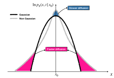
As a result, subordination processes possess an excess of probability in the tails of the PDF, compared to a Gaussian PDF with equal variance (see Fig. 1). This effect is triggered by the faster diffusers in .
On the other hand the Jensen’s inequality Rudin (1987) says that for a real-valued -measurable function on a sample space and a convex function on the real numbers we have
| (12) |
where the “” symbol means a composition of the functions. The inequality becomes strict if is strictly convex and the measure is not induced by a constant random variable. Note now that is a convex function of . Taking and , we thus have that for all time ,
| (13) | |||||
Since both and are continuous around , there must exist a neighborhood of the center in which this inequality remains valid. Thus, the non-Gaussian PDF also has an excess of probability in the central part compared to the Gaussian PDF, due to slower tracers (again, please refer to Fig. 1). The natural question to address is which of these effects is dominant when considering targeting processes.
III Subordination stochastic models
The subordination class includes a variety of stochastic models, depending on the details of the subordinator:
-
(i)
Diffusing diffusivity (DD) models Chechkin et al. (2017) are obtained assuming the diffusion coefficient to be the square of an Ornstein-Uhlenbeck process, , with
(14) The dimension of the vector is , is the autocorrelation of the process, and defines the intensity of the fluctuations. The steady-state PDF is given by
(15) where is the average diffusion coefficient. Under the name of “stochastic volatility”, these models are used in finance to correct the Black-Scholes option pricing for non-Gaussian effects Heston (1993); Fouqué et al. (2000).
Simulation of the DD model can be simply realized by updating in parallel two Ornstein-Uhlenbeck processes: The one for and the one for . In the latter, at each update the increment is drawn from a normal distribution with zero average and variance . The simulation time can be expressed in terms of and the other two free parameters are and .
-
(ii)
A concrete simple example of a subordination process is offered by a polymer in a diluted solution, exchanging monomers with a chemostat: the Grand canonical polymer (GCP) model Nampoothiri et al. (2021, 2022); Marcone et al. (2022). Indeed, the center of mass of a polymer in solution is known to diffuse with a coefficient which depends on the number of monomers as de Gennes (1979); Doi and F (1992), with the diffusion coefficient of a single monomer. The value of depends on the specific polymer model; for definiteness in this paper we adopt the Rouse value , but similar results apply to other models, such as the Zimm or the reptation ones Doi and F (1992). In the grand canonical ensemble fluctuates in time, becoming a second source of noise besides the solvent collisions responsible for the Brownian motion. can be simply modeled in terms of a birth-death process; in the mean-field limit, both the birth and death reaction rates are independent of the polymer size and their ratio corresponds to the ratio between the fugacity of the system and the critical fugacity Nampoothiri et al. (2022): As , the average polymer size becomes infinite and relative size fluctuations diverge. The steady-state size distribution is
(16) corresponding to the diffusion coefficient PMF
(17) with .
Also for the GCP model simulations are realized through a parallel update, in this case of the processes and . A simple way to simulate the birth-death process is by implementing the Gillespie algorithm Gillespie (1977) with reaction rates , . As reported for instance in Ref. Nampoothiri et al. (2022), it is possible to approximate the autocorrelation time of as
(18) where . It is clear from Eq. (18) that diverges as , a phenomenon called critical slowing down. While the ratio fixes the steady-state distribution and how close the simulation is to critical conditions, the parameter can still independently be fixed to calibrate the simulation time in terms of , according to Eq. (18). The remaining free parameter is the single-monomer diffusion coefficient .
-
(iii)
After polymerization terminates in a step-growth polymerization Odian (2004), one is left with a polydisperse sample of polymers with heterogeneous size . Assuming chains with one reaction center in the end, the size distribution coincides with Eq. (16) and it is called in this context Flory-Schulz distribution Odian (2004), with the reaction extent. In this case, must be regarded as a static random variable, , distributed according to Eq. (17).
To simulate the behavior of the Flory-Schulz polydisperse (FSP) model, for each realization one simply picks a value of with probability , and simulate then the Langevin process keeping the diffusion coefficient fixed. The statistic of the process is then obtained by averaging over the different histories. Free parameters are and .
-
(iv)
In the continuous time random walk (CTRW) Klafter and Sokolov (2011); Barkai and Burov (2020); Wang et al. (2020); Pacheco-Pozo and Sokolov (2021b) with average waiting time , one starts with a discrete subordinator , with the PMF for steps operated at time . If is a simple random walk providing the location after steps with PDF , then one gets a discrete analogous of Eq. (4):
(19) For time the typical number of steps is very large, and the operational time can be taken to be continuous, so that represents the probability for the continuous number of steps operated at time . Correspondingly, a typical random walk with finite variance tends to the Gaussian limit, recovering the subordination equation in the continuous form, Eq. (4).
Simulation of a CTRW simply proceeds as an ordinary random walk, once the value of the elapsed time taken by the update step is drawn from the assumed waiting-time distribution. Free parameters in the simulations are those defining the waiting-time distribution, in particular its average value , and the length of the random-walk step.
All these examples share the qualitative non-Gaussian features reported in Fig. 1.
IV Asymptotic regimes
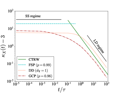
Before addressing search processes, some details about the dynamics are needed. Subordination processes may display two different regimes during which the PDF can be approximated in different ways. According to Eq. (11), the excess kurtosis evolves differently during the two regimes.
-
•
Super-statistics (SS) regime. Consider a situation in which the diffusion coefficient is almost static, , distributed according to . This approximation is exact for the FSP model, case (iii) above, but it is also valid for cases (i) and (ii) taking a heterogeneous sample of tracers initially characterized by the distribution , as long as we consider time . Indeed, for times much smaller than the autocorrelation time each tracer in the DD and GCP models basically retains its initial diffusion coefficient. Within this approximation we have
(20) and a change of variable yields
(21) From Eq. (11), the excess kurtosis is
(22) The SS regime is thus non-Gaussian; the behavior of the tracers can be characterized by operating an average of -dependent quantities, over . This “superposition of statistics” has been named in the literature super-statistics Beck and Cohen (2003); Beck (2006); Hapca et al. (2008); Wang et al. (2012), explaining the origin of the name.
-
•
Large deviation (LD) regime. With the subordinators of the DD and GCP models inherit from the Markovian evolution of a LD principle Touchette (2009):
(23) Here, “” stands for “the dominant part as ”, and is a rate function. Eq. (23) implies a time evolution of the kurtosis different from the previous one. The cumulant generating function of is defined as
(24) where is the cumulant of order of . Using Eq. (23) and the Laplace method one has
(25) with the scaled cumulant generating function Touchette (2009) of , , being time-independent. This means that within the LD approximation all the cumulants of scale linearly with time, . As a consequence, from Eq. (11) we obtain
(26) Within this regime, the central part of becomes Gaussian (central limit theorem Touchette (2009)). As time passes by, the non-Gaussian behavior is relegated to larger and larger (lesser and lesser probable) fluctuations. The probability of the scaled subordinator concentrates around its average value, and (apart from large deviations) the typical behavior is a BG diffusion with coefficient . Besides characterizing the DD and GCP models as Chechkin et al. (2017); Nampoothiri et al. (2021, 2022); Marcone et al. (2022), one can directly calculate that the CTRW, with an exponential waiting time distribution satisfies a LD principle Pacheco-Pozo and Sokolov (2021b) and Eq. (26) (namely, ), for all time .
Fig. 2 displays the time evolution of the excess kurtosis for the different models, highlighting the two regimes.
V Non-Gaussian and Gaussian targeting
Let us now consider two classic targeting problems in one dimension:
-
a)
Finite interval with absorbing boundaries at the extrema.
-
b)
Semi-infinite domain with absorbing boundary at .
For ordinary diffusion, exact expressions Redner (2001) are available for the (cumulative) probability of reaching a target by time , given the initial position and the diffusion coefficient ,
| (27) |
( is the survival probability):
-
a)
For the finite interval,
(28) implying
(29) -
b)
For the semi-infinite domain,
(30) yielding
(31)
The time derivative of these expressions provides the PDF for reaching the boundary at time , , from which one can obtain the characteristic time for a single particle to reach the target, :
-
a)
With the finite domain, is naturally given by the mean first passage time,
(32) -
b)
The mean first passage time of the semi-infinite domain is infinite; however, a characteristic time can still be identified as Redner (2001)
(33) for .
Given the two dynamical regimes discussed above, it is meaningful to contemplate the probability associated with the SS regime,
| (34) | |||||
| (35) |
and the one corresponding to the LD regime,
| (36) |
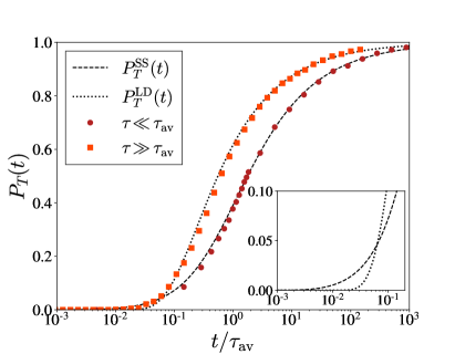
According to Fig. 2 the behavior of the FSP model is characterized by the probability while the CTRWs for are ruled by . For the DD model and the GCPs the actual probability will be close to for and will tend to as . In Fig. 3 we highlight the two regimes for the GCP model with the semi-infinite domain; a similar plot is valid for the DD model Sposini et al. (2019). The abscissa is rescaled by the characteristic time for the particle with an average diffusion coefficient to travel over the distance from the target, namely
| (37) |
As shown above, is a convex function of . Taking now , and again , the Jensen’s inequalityRudin (1987) conveys the following basic result:
| (38) |
Since Jensen’s inequality is valid when averaging on general distributions, Eq. (38) applies to the DD and the GPC models, and also for CTRWs if we compare the early behavior ruled by the discrete subordination formula, Eq. (19), with the LD Gaussian limit, attained for . We thus conclude, consistently with earlier specific findings Lanoiselée et al. (2018); Grebenkov (2019); Sposini et al. (2019), that for a single searcher within the general class of non-Gaussian diffusion processes based on subordination, the characteristic time to target is larger than in ordinary diffusion. As the characteristic time to target in ordinary diffusion is in general inversely related to , this finding extends to general transient regimes and targeting processes, not necessarily one-dimensional. It is an effect due to the excess of probability in the central part of the PDF (slower diffusers) (see Fig. 1) and it is somehow at odds with the general prospect of surprising phenomena triggered by rare fluctuations Wang et al. (2012).
What about the “tail effect” in Fig. 1? By inspecting and , one finds that typically the latter is larger than the former, consistently with Eq. (38). However, a closer look reveals that the “tail effect” dominates at time shorter than (Fig. 3, inset), with being the solution of
| (39) |
The corresponding fraction of successful single-particle searches below which non-Gaussian chases are more efficient than the BG ones is typically small; for instance and in Fig. 3. However, this apparently negligible effect makes a drastic difference in extreme first passage problems, where a small fraction of the total number of searchers is required to first reach the target to activate a certain function. This finding is discussed in details in the companion paper, Ref. Sposini et al. (2023).
VI Conclusions
Targeting of receptors by ligand particles is a fundamental biological mechanism used by cells to activate or stop specific functions. The mechanism makes use of the diffusive properties of the ligands and the basic quantity to measure is the characteristic time employed by a searcher to reach the target, i.e., when it exists finite, the mean first passage time. Since recent experiments and simulations highlighted heterogeneous conditions in which diffusion becomes Brownian non-Gaussian, the question arose whether non-Gaussianity enhances or not searches.
While this issue has already been addressed for specific models Lanoiselée et al. (2018); Grebenkov (2019); Sposini et al. (2019), here we have provided a general approach valid for all Brownian non-Gaussian processes based on subordination. Using Jensen’s inequality and the positiveness of the variance of the subordinator, we have demonstrated that the distributions of subordinated diffusive particles display an excess of probability both in the central part and in the tails, when compared with Gaussians. The qualitative features appearing in Fig. 1 are independent of the kind of subordinator. At variance, the dynamical regimes shown in Fig. 2 depend on the specific definition of the subordinator. The DD and GCP models display both the SS and the LD regimes. The FSP model is characterized by the SS regime only, and the CTRW model with exponential waiting times possesses exclusively the LD regime.
In agreement with earlier findings, we have shown on general ground that the “central effect” dominates the one-particle searching process, making the characteristic time to target larger than in ordinary Gaussian diffusion. This conclusion encompasses current models of Brownian non-Gaussian diffusion and implies that, for ordinary diffusion-limited-reaction scenarios, non-Gaussianity weakens reaction rates.
The “tail effect” pertains to the realm of rare events and control instead, extreme searches, where only a few among many diffusers are required to reach the target. In Ref. Sposini et al. (2023) it is shown that this is the context in which non-Gaussianity makes a substantial difference.
Acknowledgments
F.S. and F.B. acknowledge the support by the project MUR-PRIN 2022ETXBEY, ”Fickian non-Gaussian diffusion in static and dynamic environments”, funded by the European Union – Next Generation EU”’. V.S. acknowledges the support from the European Commission through the Marie Skłodowska-Curie COFUND project REWIRE, grant agreement No. 847693. A.C. acknowledges the support of the Polish National Agency for Academic Exchange (NAWA).
References
- Wang et al. (2009) B. Wang, S. M. Anthony, S. C. Bae, and S. Granick, Proceedings of the National Academy of Sciences 106, 15160 (2009).
- Wang et al. (2012) B. Wang, J. Kuo, S. C. Bae, and S. Granick, Nature materials 11, 481 (2012).
- Toyota et al. (2011) T. Toyota, D. A. Head, C. F. Schmidt, and D. Mizuno, Soft Matter 7, 3234 (2011).
- Yu et al. (2013) C. Yu, J. Guan, K. Chen, S. C. Bae, and S. Granick, ACS Nano 7, 9735 (2013).
- Yu and Granick (2014) C. Yu and S. Granick, Langmuir 30, 14538 (2014).
- Chakraborty and Roichman (2020) I. Chakraborty and Y. Roichman, Physical Review Research 2, 022020 (2020).
- Weeks et al. (2000) E. R. Weeks, J. C. Crocker, A. C. Levitt, A. Schofield, and D. A. Weitz, Science 287, 627 (2000).
- Wagner et al. (2017) C. E. Wagner, B. S. Turner, M. Rubinstein, G. H. McKinley, and K. Ribbeck, Biomacromolecules 18, 3654 (2017).
- Jeon et al. (2016) J.-H. Jeon, M. Javanainen, H. Martinez-Seara, R. Metzler, and I. Vattulainen, Physical Review X 6, 021006 (2016).
- Yamamoto et al. (2017) E. Yamamoto, T. Akimoto, A. C. Kalli, K. Yasuoka, and M. S. Sansom, Science advances 3, e1601871 (2017).
- Stylianidou et al. (2014) S. Stylianidou, N. J. Kuwada, and P. A. Wiggins, Biophysical journal 107, 2684 (2014).
- Parry et al. (2014) B. R. Parry, I. V. Surovtsev, M. T. Cabeen, C. S. O’Hern, E. R. Dufresne, and C. Jacobs-Wagner, Cell 156, 183 (2014).
- Munder et al. (2016) M. C. Munder, D. Midtvedt, T. Franzmann, E. Nuske, O. Otto, M. Herbig, E. Ulbricht, P. Müller, A. Taubenberger, S. Maharana, et al., elife 5, e09347 (2016).
- Cherstvy et al. (2018) A. G. Cherstvy, O. Nagel, C. Beta, and R. Metzler, Physical Chemistry Chemical Physics 20, 23034 (2018).
- Li et al. (2019) Y. Li, F. Marchesoni, D. Debnath, and P. K. Ghosh, Physical Review Research 1, 033003 (2019).
- Cuetos et al. (2018) A. Cuetos, N. Morillo, and A. Patti, Physical Review E 98, 042129 (2018).
- Hapca et al. (2008) S. Hapca, J. W. Crawford, and I. M. Young, Journal of the Royal Society Interface 6, 111 (2009).
- Pastore et al. (2021) R. Pastore, A. Ciarlo, G. Pesce, F. Greco, and A. Sasso, Physical Review Letters 126, 158003 (2021).
- Pastore and Raos (2015) R. Pastore and G. Raos, Soft Matter 11, 8083 (2015).
- Miotto et al. (2021) J. M. Miotto, S. Pigolotti, A. V. Chechkin, and S. Roldán-Vargas, Physical Review X 11, 031002 (2021).
- Rusciano et al. (2022) F. Rusciano, R. Pastore, and F. Greco, Physical Review Letters 128, 168001 (2022).
- Lanoiselée et al. (2018) Y. Lanoiselée, N. Moutal, and D. S. Grebenkov, Nat. Comm. 9, 4398 (2018).
- Grebenkov (2019) D. S. Grebenkov, J. Phys. A 52, 174001 (2019).
- Sposini et al. (2019) V. Sposini, A. Chechkin, and R. Metzler, Journal of Physics A: Mathematical and Theoretical 52, 04LT01 (2019).
- Chechkin et al. (2017) A. V. Chechkin, F. Seno, R. Metzler, and I. M. Sokolov, Physical Review X 7, 021002 (2017).
- Nampoothiri et al. (2021) S. Nampoothiri, E. Orlandini, F. Seno, and F. Baldovin, Physical Review E 104, L062501 (2021).
- Nampoothiri et al. (2022) S. Nampoothiri, E. Orlandini, F. Seno, and F. Baldovin, New J. Phys. 24, 023003 (2022).
- Marcone et al. (2022) B. Marcone, S. Nampoothiri, E. Orlandini, F. Seno, and F. Baldovin, J. Phys. A: Math. Theor. 55, 354003 (2022).
- Flory (1953) P. Flory, Principles of Polymer Chemistry (Cornell University Press, 1953).
- Cosgrove (2005) T. Cosgrove, Colloid Science Principles, Methods and Applications (Blackwell Publishing, Oxford, UK, 2005).
- Odian (2004) G. Odian, Principles of Polymerization (John Wiley & Sons, 2004).
- Klafter and Sokolov (2011) J. Klafter and I. Sokolov, First Steps in Random Walks: From Tools to Applications (Oxford University Press, 2011).
- Barkai and Burov (2020) E. Barkai and S. Burov, Physical Review Letters 124, 060603 (2020).
- Wang et al. (2020) W. Wang, E. Barkai, and S. Burov, Entropy 22, 697 (2020).
- Pacheco-Pozo and Sokolov (2021a) A. Pacheco-Pozo and I. M. Sokolov, Physical Review Letters 127, 120601 (2021a).
- Pacheco-Pozo and Sokolov (2021b) A. Pacheco-Pozo and I. M. Sokolov, Physical Review E 103, 042116 (2021b).
- Rudin (1987) W. Rudin, Real and complex analysis (McGraw-Hill, 1987).
- Sposini et al. (2023) V. Sposini, S. Nampoothiri, A. Chechkin, E. Orlandini, F. Seno, and F. Baldovin, Physical Review Letters 132, 117101 (2024).
- Feller (1968) W. Feller, An Introduction to Probability Theory and Its Applications (John Wiley & Sons, 1968).
- Bochner (2020) S. Bochner, Harmonic analysis and the theory of probability (University of California press, 2020).
- Heston (1993) S. Heston, Rev. Financial Studies 6, 327 (1993).
- Fouqué et al. (2000) J.-P. Fouqué, G. Papanicolaou, and K. Sircar, Derivatives in Financial Markets with Stochastic Volatility (Cambridge University Press, Cambridge, England, 2000).
- de Gennes (1979) P.-G. de Gennes, Scaling Concepts in Polymer Physics (Cornell University Press, 1979).
- Doi and F (1992) M. Doi and E. S. F, The Theory of Polymer Dynamics (Oxford University Press, 1992).
- Gillespie (1977) D. T. Gillespie, Journal of Physical Chemistry 81, 2340–2361 (1977).
- Beck and Cohen (2003) C. Beck and E. G. Cohen, Physica A: Statistical mechanics and its applications 322, 267 (2003).
- Beck (2006) C. Beck, Progress of Theoretical Physics Supplement 162, 29 (2006).
- Touchette (2009) H. Touchette, Physics Reports 478, 1 (2009).
- Redner (2001) S. Redner, A guide to first passage processes (Cambridge University Press, 2001).