Measurement of groomed event shape observables in deep-inelastic electron-proton scattering at HERA

Abstract

The H1 Collaboration at HERA reports the first measurement of groomed event shape observables in deep inelastic electron-proton scattering (DIS) at $\sqrt{s}=319~{}$GeV, using data recorded between the years 2003 and 2007 with an integrated luminosity of 351 $\mathrm{pb}^{-1}$. Event shapes provide incisive probes of perturbative and non-perturbative QCD. Grooming techniques have been used for jet measurements in hadronic collisions; this paper presents the first application of grooming to DIS data. The analysis is carried out in the Breit frame, utilizing the novel Centauro jet clustering algorithm that is designed for DIS event topologies. Events are required to have squared momentum-transfer $Q^{2}>150$ GeV² and inelasticity $0.2<y<0.7$. We report measurements of the production cross section of groomed event 1-jettiness and groomed invariant mass for several choices of grooming parameter. Monte Carlo model calculations and analytic calculations based on Soft Collinear Effective Theory are compared to the measurements.

1 Introduction

Event shape observables characterize the distribution of final-state particles produced in high-energy particle interactions. Event shapes have been measured extensively in $e^{+}e^{-}$ collisions [1, 2, 3, 4, 5, 6, 7, 8, 9, 10, 11, 12] and in $ep$ collisions [13, 14, 15, 16, 17]; such observables are calculable to high precision using perturbative Quantum Chromodynamics (pQCD) [18, 19, 20, 21, 22]. Event shapes are incisive probes of QCD, notably to constrain the strong coupling constant $\alpha_{s}$ [9, 23, 24, 25, 26, 27, 28, 29]. The description of hadronic final states in Monte Carlo event generators has likewise benefitted substantially from event shape measurements [7, 18, 30, 31, 32, 33].

Jets arise from energetic partons (quarks and gluons) produced in hard interactions. The partons are initially highly virtual, decaying in a partonic shower that is experimentally observable as a correlated spray of hadrons. Jets provide a laboratory for testing QCD [34]. However, the precision of jet measurements at hadron colliders is limited by the contribution of non-perturbative (NP) processes and by the presence of the underlying event, which consists of final-state particles that do not originate from the hard-scattering process that produced the jet being studied. This limitation is addressed by the application of jet grooming algorithms [35, 36, 37, 38, 39, 40, 41, 42], which systematically removes particles likely to originate in NP processes and the underlying event, in a way that is theoretically and experimentally well-controlled [43].

In jet grooming algorithms, typically the Cambridge-Aachen [44] sequential recombination algorithm is applied, which combines hard jet constituents (particle four-vectors) into a jet in the first recombination steps, and soft and wide-angle particles in later steps. The recombination sequence is then inspected in reverse. For each step in this inspection the kinematics of its contributing branches are compared to a specified condition; for instance, the ratio $z_{\mathrm{g}}$ of the transverse momentum ($p_{\mathrm{T}}$) of the softer branch to the summed $p_{\mathrm{T}}$ of both branches is required to satisfy $z_{\mathrm{g}}>z_{\mathrm{cut}}$, for a given value of $z_{\mathrm{cut}}$. If this condition is not satisfied, the softer branch is discarded from the event (hence the term “grooming”) and the comparison continues to the next recombination step along the harder branch until the condition is satisfied. If no recombination step satisfies the condition, the event is discarded. The choice of condition differentiates jet grooming algorithms [43].

The technique of jet grooming has been applied extensively in proton-proton ($pp$) collisions at the Large Hadron Collider and at the Relativistic Heavy Ion Collider, for instance to search for the decay of boosted heavy particles, discriminate jets initiated by quarks or gluons, or measure jet substructure [45, 46, 47, 48, 49, 50, 51, 52, 53, 54, 55, 56, 57, 58, 43]. Jet grooming has also been used to study the modification of jets propagating in the Quark-Gluon Plasma generated in heavy-ion collisions [59, 49, 60, 61, 62, 63].

Jets have also been measured extensively in $e^{+}e^{-}$ [64, 65, 66, 67, 68, 69, 9] and lepton-proton deep inelastic scattering (DIS) [70, 71, 72, 73, 74, 75, 76, 77, 78, 79, 80, 81, 82, 83, 84, 85, 86, 87, 88]. The underlying event background in such collision systems is smaller than in $pp$ collisions, enabling more accurate measurement of soft components of jets. In addition, the kinematic properties of the partonic scattering are known experimentally, providing more precise comparison to QCD calculations. To date, grooming has not been applied to data from $ep$ DIS.

It was recently proposed to apply grooming algorithms not only to jet measurements at hadron colliders, but also to full events in $ep$ DIS [89], leveraging the similarities between DIS at high virtualities and single jets. From a theoretical standpoint, groomed observables in $ep$ DIS are free of non-global logarithms [89, 22, 90, 91] and have reduced hadronization effects relative to ungroomed observables [38, 90]. In addition, the magnitude of the non-perturbative component of such observables is controllable experimentally by varying the strength of the grooming parameter $z_{\mathrm{cut}}$ [38, 89, 90].

In this paper, the H1 Collaboration at HERA reports the first measurement of groomed event shapes in $e^{-}p$ and $e^{+}p$ neutral-current (NC) deep inelastic scattering (electrons and positrons are referred to generically as “electrons” in the following). The data were recorded during the years 2003 to 2007 with electron and proton beam energies of $E_{e}=27.6$ GeV and $E_{p}=920$ GeV, respectively, corresponding to $\sqrt{s}=319$ GeV. The recorded dataset has integrated luminosity $\mathcal{L}_{\mathrm{int}}=351~{}\mathrm{pb}^{-1}$. The analysis is based on events with exchanged-boson virtuality $Q^{2}>150$ GeV² and inelasticity $0.2<y<0.7$. We report measurements of the production cross section of groomed event 1-jettiness and groomed event invariant mass for several choices of grooming parameter $z_{\mathrm{cut}}$. Monte Carlo model calculations and analytic calculations based on Soft Collinear Effective Theory (SCET) [89] and NNLO+NLL^′ pQCD [18] are compared to the measurements.

These data provide new, differential constraints on the detailed structure of DIS-induced final states, which are valuable for the tuning of MC event generators. Improvement of such event generators is important, for instance, for the physics program of the future Electron-Ion Collider [92].

The paper is organized as follows: Section 2 describes the experimental apparatus and dataset; Section 3 presents theoretical calculations that are compared to the data; Section 4 outlines the analysis procedure and event selection; Section 5 presents the corrections applied to the data; Section 6 presents the uncertainties; Section 7 reports results of the analysis and the comparison of theoretical predictions to the measurements; and Section 8 provides a summary.

2 Experimental Setup

The H1 experiment is a general purpose particle detector with full azimuthal coverage around the electron-proton interaction region [93, 94, 93, 95, 96, 97]. The detector is described in Refs. [98, 99, 97, 100]. H1 employs a right-handed coordinate system in which the proton beam direction defines the positive $z$ direction. The nominal $ep$ interaction point is located at $z=0$.

The liquid argon calorimeter (LAr) [101, 102], which provides a trigger for high-$Q^{2}$ neutral current DIS, subtends polar angles of $4^{\circ}<\theta<154^{\circ}$ and provides an energy resolution of $\sigma(E)/E\simeq(11\%/\sqrt{E/\mathrm{GeV}})\oplus 1\%$ for electrons and $\sigma(E)/E\simeq(55\%/\sqrt{E/\mathrm{GeV}})\oplus 3\%$ for charged pions. The central tracking system, comprising gaseous drift and proportional chambers and a silicon vertex detector, covers the polar range $15^{\circ}<\theta<165^{\circ}$ and has transverse momentum resolution for charged particles $\sigma(p_{\mathrm{T}})/{p_{\mathrm{T}}}\simeq 0.2\%\cdot p_{\mathrm{T}}/\mathrm{GeV}\oplus 1.5\%$. A lead-scintillating fiber calorimeter (SpaCal) [94, 103], consisting of both electromagnetic and hadronic sections, covers the backward direction ($153^{\circ}<\theta<177^{\circ}$). The SpaCal has electromagnetic energy resolution of $\sigma(E)/{E}\simeq(7.5\%/\sqrt{E/\mathrm{GeV}})\oplus 2\%$.

Events are triggered by requiring a high-energy cluster in the electromagnetic portion of the LAr. The trigger and event selection used in the analysis closely follows Ref. [87]. The efficiency of the trigger is greater than $99\%$ in the phase space of this analysis. Events are further selected online by requiring the scattered electron to have an energy greater than 11 GeV and to fall within the LAr fiducial volume.

In the offline analysis, an energy flow algorithm combines information from the tracking detectors and calorimeters to generate a set of four-vectors [104, 105, 106]. These four-vectors are used to define the scattered electron and the hadronic final state (HFS). Isolated energy deposits with high energy in the backward and central sections of the electromagnetic calorimeters are typically the result of QED radiation of a photon off the electron. If the energy deposit is closer to the scattered electron than the electron beam direction, the photon is likely to come from final-state radiation and its four-vector is recombined with the four-vector of the scattered electron. If the photon is closer to the electron beam ($-z$) direction, it is likely the result of initial-state radiation (ISR) and is removed from the event. The HFS is defined as all the particles remaining after this procedure, excluding the scattered electron.

The kinematic variables describing the event, $Q^{2}$, $y$, and Bjorken $x$ (denoted $x_{\mathrm{Bj}}$), are reconstructed using the $I\Sigma$ method as described in Ref. [107]. Bjorken $x_{\mathrm{Bj}}=Q^{2}/(2P\cdot q)$, where $P$ and $q$ refer to the incoming proton and exchanged boson four-vectors, respectively. The inelasticity $y=P\cdot q/P\cdot k$, where $k$ is the incoming electron four-vector. These kinematic variables are used to reconstruct the boost to the Breit frame, as well as the vector defining the current hemisphere of the Breit frame, $q_{J}=xP+q$. The definitions of the Breit frame and $q_{J}$ are described in more detail in Section 4.

Events are further selected based on the following quality assurance cuts placed on quantities measured in the laboratory frame:

• The measured $z$-location of the event vertex is constrained to be within 35 cm of the nominal vertex $z$-location.

• The total longitudinal momentum balance ($E-p_{z}$) of the event, evaluated by summing the $E-p_{z}$ of all measured particles, is required to satisfy $50<E-p_{z}<60$ GeV. This requirement predominantly serves to reduce the contribution from events with significant QED initial-state radiation and events likely to come from photoproduction or beam-gas background. It has the additional benefit of rejecting events in which the hadronic final state is poorly reconstructed.

• The total transverse momentum ($p_{\mathrm{T}}$) of the hadronic final state is required to approximately balance that of the scattered electron $p_{\mathrm{T}}$, $0.6<{p_{\mathrm{T,HFS}}}/{p_{\mathrm{T},e}}<1.6$ and ${p_{\mathrm{T,HFS}}}-{p_{\mathrm{T},e}}<5$ GeV. These requirements ensure that the hadronic final state and scattered electron are well-measured.

• The vector defining the current hemisphere of the Breit frame, $q_{J}$, is required to have a polar angle $7^{\circ}<\theta_{q_{J}}<175^{\circ}$ in the lab frame in order to suppress non-collision backgrounds and to ensure the hadronic final state is properly contained within the detector.

• Events with $\theta_{q_{J}}>149^{\circ}$ and the velocity of the Lorentz boost to the Breit frame $\beta>0.9$ are rejected to suppress contamination from initial-state QED radiation. Events in which the difference between the polar angles of the HFS and the current hemisphere vector satisfies $\theta_{q_{J}}-\theta_{\mathrm{HFS}}>90^{\circ}$ are also rejected for the same reason.

• In the kinematic region studied here, the hadronic final state and the scattered electron are typically produced at similar polar angles. Events events with $Q^{2}<700$ GeV² and $|\Delta\eta|>0.3$ are poorly measured and are rejected, where pseudorapidity in the laboratory frame $\eta=-\mathrm{ln}(\mathrm{tan}\frac{\theta}{2})$, and $\Delta\eta$ is the difference between the hadronic final state and the scattered electron.

After the kinematic phase space selection and the above event criteria are enforced, the analysed dataset consists of 189,106 events.

3 Simulations and theoretical calculations

Calculations based on the following Monte Carlo event generators and QCD calculations are compared to the data:

• Djangoh 1.4 [108, 109, 110] uses Born-level matrix elements for NC DIS and dijet production, combined with the color dipole model from Ariadne [111] for higher-order emissions. Djangoh includes an interface to HERACLES [109] for higher-order QED effects at the lepton vertex. The proton parton distribution function (PDF) used by Djangoh is CTEQ6L [112]. Hadronization is simulated with the Lund hadronization model [113, 114], using parameters tuned to data by the ALEPH Collaboration [9].

• Rapgap 3.1 [115] implements Born-level matrix elements for NC DIS and dijet production and uses the leading logarithmic approximation for parton showering. The PDF set and hadronization model used in Rapgap are the same as used in Djangoh.

• The MC event generator Pythia 8.307 [116, 117] is used with two different parton-shower models: the default dipole-like $p_{\perp}$-ordered shower and the Dire [118, 119, 120] parton shower, which is an improved dipole shower with additional handling of collinear enhancements. Both implementations use the Pythia 8.3 default for hadronisation [117], which is based on the Lund string model. The parton showers both use 0.118 for value of the strong coupling constant at the mass of the $Z$ boson, and both variations considered here use MMHT2014 as the hard PDF [121].

• A recent prediction from Ref. [122] generalizes the POWHEG method to DIS, including handling of initial-state radiation off the lepton beam. This prediction, denoted Pythia+POWHEG, includes predictions in NLO QCD matched to parton showers using the POWHEG method [123, 124], which are then interfaced to Pythia 8.303. The default Pythia shower and hadronization schemes are applied. The Frixione-Kunszt-Signer (FKS) subtraction technique [125] is used to parameterize the radiation phase space.

• The MC event generator Herwig 7.2 [126] is also studied in three variants. For the default prediction, Herwig 7.2 implements leading-order matrix elements that are supplemented with an angular-ordered parton shower [127] and the cluster hadronization model [128, 129]. The second variant makes use of the MC@NLO method that implements NLO matrix element corrections. In addition, a matching with the default angular-ordered parton shower is performed [130]. The third variant also makes use of NLO matrix elements but applies the dipole merging technique and a dipole parton shower [130]. The PDF used for all three of the Herwig variations is MMHT2014 [121]. The events generated with Herwig are further processed with Rivet [131].

• Predictions are obtained with Sherpa 2 [132, 133], where Comix [134] generates matrix elements for up to three final-state jets. The CKKW merging formalism [135] is used to augment these jets with dipole showers [136, 137], and the final-state partons are hadronized with cluster hadronization as implemented in AHADIC++ [138]. As an alternative prediction, the hadronization step is performed with the Lund string fragmentation model [139]. Both predictions use the Sherpa 2 default PDF, which is CT10 [140].

• A set of predictions for the groomed 1-jettiness is provided by the Sherpa authors using a pre-release version of Sherpa 3. Sherpa 3 features a new cluster hadronization model, described in Ref. [141]. Matrix elements at NLO are obtained from OpenLoops [142], and the resulting partons are showered via the Sherpa dipole shower [137] based on the truncated shower method described in Refs. [143, 144]. Sherpa 3 additionally features intrinsic $k_{\mathrm{T}}$ of the partons within the proton, while the predictions from Sherpa 2 have no intrinsic $k_{\mathrm{T}}$ included. The model for partonic intrinsic $k_{\mathrm{T}}$ used in the Sherpa 3 prediction is a Gaussian form with mean of 0 GeV and $\sigma=0.75$ GeV. The prediction has an associated uncertainty, defined as the extrema of a 7-point scale variation.

• Another prediction at NNLO+NLL^′ [18] is provided for the groomed 1-jettiness. The predictions are computed using the CAESAR formalism [145] for NLL resummation as implemented in the Sherpa [132] framework [146, 147] and extended to cover the case of soft-drop groomed event shapes in Refs. [29, 148]. The resummed results are matched to fixed order predictions at NNLO accuracy, derived with the techniques implemented in Sherpa in Ref. [149]. Via a multiplicative matching, the calculation achieves NNLO+NLL^′ accuracy. A description of the full setup in the DIS case can be found in Ref. [18]. Non-perturbative corrections are applied via a transfer matrix approach [150] from Sherpa tuned to data from the LEP and HERA experiments [141, 18]. The same techniques for calculating the groomed invariant mass are used here for the first time. Care is taken to evaluate logarithms of the form $\ln(M^{2}/Q^{2})$ to avoid ambiguities arising from the normalisation of the observable. The calculation ultimately achieves the same NNLO+NLL^′ accuracy as before.

• Predictions for the groomed invariant mass are provided using the formalism of SCET [89]. Predictions are constructed at NNLL for the shape of the groomed invariant mass spectrum in the single-jet limit, corresponding to small values of the groomed invariant mass $M_{\text{Gr.}}^{2}$$\ll$ $Q^{2}$. The perturbative predictions are convoluted with a shape function to account for non-perturbative effects. The predictions are provided at two values of the shape function mean parameter, $\Omega_{\mathrm{NP}}$. No attempt is made to match the NNLL calculation to a fixed-order prediction.

4 Observables

4.1 Breit frame

The reported measurements are carried out in the Breit frame of reference [151]. The Breit frame is the reference frame in which

$$2x_{\mathrm{Bj}}\vec{P}+\vec{q}=0,$$ (1)

where $\vec{P}$ is the three-momentum of the incoming proton beam and $\vec{q}$ is the three-momentum of the exchanged boson. As for the laboratory frame of reference, we choose the positive $z$ axis of the Breit frame to be the direction of the incoming proton. In the quark-parton model, the Breit frame is the frame of reference in which the struck parton is initially aligned with the $z$ axis with $p_{z}=Q/2$ and leaves along the same axis with $p_{z}=-Q/2$ after the momentum transfer from the space-like virtual boson. The maximum available longitudinal momentum in the Breit frame is therefore $Q/2$, and at Born level the scattered parton has transverse momentum $p_{\mathrm{T}}=0$.

The direction of the proton remnant is defined as $\eta_{\mathrm{{}_{Breit}}}=+\infty$, while the direction of the struck parton is defined as $\eta_{\mathrm{{}_{Breit}}}=-\infty$. The region $\eta_{\mathrm{{}_{Breit}}}>0$ is denoted the remnant hemisphere (RH), and the $\eta_{\mathrm{{}_{Breit}}}<0$ region is denoted the current hemisphere (CH). Events with large $p_{\mathrm{T}}$ in the Breit frame therefore correspond to multi-jet topologies, e.g. QCD Compton scattering in which the quark recoils with significant $p_{\mathrm{T}}$ from a hard gluon emission. For the kinematic selection used in this analysis, namely $Q^{2}>150$ GeV² and inelasticity $0.2<y<0.7$, the scattered electron is typically at mid-rapidity ($\eta_{\mathrm{{}_{Breit}}}\sim 0$) in the Breit frame. This phase space also corresponds to the region in which the magnitude of the Lorentz boost from the lab frame to the Breit frame is small, thus minimizing the event-to-event change in the detector acceptance in the Breit frame [152].

4.2 Jet and event clustering in the Breit frame: Centauro algorithm

In the HERA convention, the leading-order quark-parton model process $eq\rightarrow eq$ produces a jet at $\eta_{\mathrm{{}_{Breit}}}=-\infty$ in the Breit frame. Such jets will not be captured by longitudinally-invariant $k_{\mathrm{T}}$-type sequential recombination clustering algorithms applied in that frame [152, 153], since those algorithms cluster based on the transverse component of particle momenta that is largely boosted away by the transformation to the Breit frame. Additionally, the distance $d_{ij}$ between particles becomes large in the direction of the struck parton due to the factor $R^{2}=\sqrt{\Delta\eta_{\mathrm{Breit}}^{2}+\Delta\phi^{2}}$ in the denominator of the distance metric for those algorithms.

Centauro [153] is a sequential-recombination jet algorithm that overcomes these limitations by means of an asymmetric clustering measure, which preferentially clusters a jet from radiation in the current hemisphere of the Breit frame. Centauro thus clusters the Born-level configuration into a jet more readily than other laboratory and Breit frame algorithms. The Centauro distance measure is

$$d_{ij}=(\Delta\bar{\eta}_{ij})^{2}+2\bar{\eta}_{i}\bar{\eta}_{j}(1-\cos(\Delta\phi_{ij})),$$ (2)

where

$$\bar{\eta}_{i}=-\frac{2p_{\mathrm{T},i}}{p_{z,i}},$$ (3)

in the Breit frame, and $\Delta\phi_{ij}$ is the azimuthal angle difference between pairs of objects that are candidates for clustering.

The Centauro algorithm can be used as a traditional jet-finding algorithm to reconstruct jets, but it can also be applied to the entire DIS event (equivalent to setting the jet radius $R\rightarrow\infty$) to generate a clustering tree in which the last clustered radiation is farthest from the nominal struck parton direction in the Breit frame. As discussed in Ref. [89], the natural quantity for comparison of branches in this tree is the Lorentz-invariant momentum fraction $z_{i}$,

$$z_{i}=\frac{P\cdot p_{i}}{P\cdot q},$$

which in the Breit frame represents the fraction of the virtual boson momentum carried by the object $i$. Branches of the tree with low $z_{i}$ are either soft or at wide angles with respect to the virtual boson. Branches with high $z_{i}$ are likely to be fragments of the struck parton.

4.3 Event grooming

Event grooming follows the procedure described in Ref. [89], as follows. All four-vectors in the event are clustered into a tree by the Centauro algorithm; the tree is iteratively declustered in order reverse to the initial clustering; and at each declustering step the values of $z_{i}$ of the branches are compared to the grooming condition,

$$\frac{\text{min(}z_{i},z_{j})}{z_{i}+z_{j}}>z_{\mathrm{cut}}.$$ (4)

If the grooming condition is not met, the branch with smaller $z_{i}$ is removed and the remaining branch is again subdivided and compared to the grooming condition. The procedure continues until the grooming condition is met. Events in which the algorithm queries the full clustering tree without the grooming condition being met are removed from the analysis and do not contribute to the measured event shape cross section. The fraction of events which do not pass the grooming condition naturally increases with $z_{\mathrm{cut}}$. This approach is a version of the modified MassDrop Tagger (mMDT) grooming algorithm with $\beta=0$ [90], adapted for DIS with $z_{i}$ playing the role of $p_{\mathrm{T}_{i}}$ in standard mMDT.

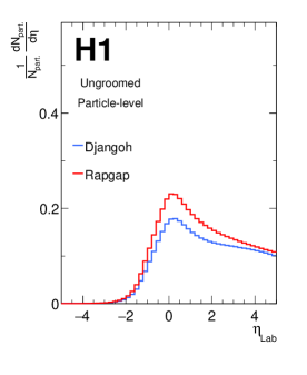
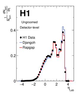
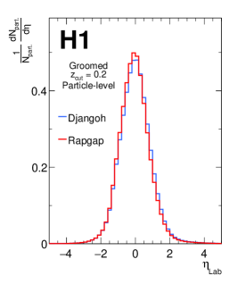
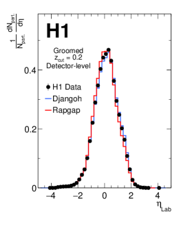
Figure 1: Normalized distribution of particles measured in data and simulated by Djangoh and Rapgap, as a function of pseudorapidity in the laboratory frame. Left: particle-level; right: detector-level. Upper: ungroomed ($z_{\mathrm{cut}}$=0); lower: groomed with $z_{\mathrm{cut}}$=0.2.

Figure 1 shows single-particle pseudorapidity distributions for groomed and ungroomed events at both particle- and detector-level. “Particle-level" here refers to the quantities produced by the event generator, where the final state comprises particles with proper lifetime greater than 8 ns. “Detector-level" refers to the four-vectors reconstructed after the particles from the generator are passed through a GEANT [154] detector simulation program, as well as several reconstruction algorithms. The complex shape of the ungroomed detector-level pseudorapidity distribution in the top right panel of Fig. 1 can be attributed to the transition between the barrel and forward sections of the LAr, as well as the contribution of secondary interactions in the detector and beamline.

Figure 1 also compares the detector-level simulated distributions to raw data, with good agreement found. For the data, the fraction of accepted events that pass the grooming cut is 99.3% for $z_{\mathrm{cut}}$= 0.05, 98.4% for $z_{\mathrm{cut}}$= 0.1, and 92.7% for $z_{\mathrm{cut}}$= 0.2.

4.4 Groomed event shapes

Classical global event shape observables incorporate a summation over all particles in an event, including those which are produced at small angles with respect to the beam. Monte Carlo simulations show that, for high-$Q^{2}$ $ep$ DIS events such as those in this analysis, 30–40% of generated particles fall in the forward region $\eta_{\mathrm{{}_{Lab}}}>3.5$, beyond the detector acceptance. In previous event shape analyses at HERA [13, 14, 15, 16, 17], the impact of the missing forward acceptance was reduced by limiting the measurement to particles in the current hemisphere, which are better contained by the detector. In that case, however, theoretical calculations of event shapes must also include radiation that is nominally emitted in the remnant hemisphere but enters the current hemisphere at higher order, generating non-global logarithms that can compromise theoretical precision [155, 89]. These limitations motivate consideration of methods that can ameliorate both the experimental and theoretical challenges typically associated with event shape observables.

It can be seen from Fig. 1 that the application of grooming alleviates the need for a redefinition of event shape observables, since the grooming procedure grooms away the particles produced outside the detector acceptance. This follows from the fact that at high $Q^{2}$, the exchanged virtual boson typically points toward the central region of the detector. Since the grooming tends to remove particles that are anti-collinear and at wide angles with respect to the exchanged boson, the particles that survive the grooming are generally well-contained within the central region of the detector. For the hardest grooming cut considered here, $z_{\mathrm{cut}}\ =0.2$, only 0.5% of particles surviving the grooming at particle-level are beyond the forward acceptance of the detector. QCD initial-state radiation, beam remnants, and wide-angle soft radiation are largely groomed away. The remaining particles therefore consist predominantly of fragments of the struck parton, which are collimated in the virtual boson direction. Groomed event shape observables are calculated from these surviving particles.

This paper reports two groomed event shape observables: $M_{\text{Gr.}}^{2}$, the groomed invariant mass, and $\tau^{b}_{1,{\text{Gr.}}}$, the groomed 1-jettiness. The observable $M_{\text{Gr.}}^{2}$ is defined as

$$M_{\text{Gr.}}^{2}=\left(\sum_{i\in\mathrm{groomed}(z_{\mathrm{cut}})}p_{i}\right)^{2},$$ (5)

where the sum over $i$ runs over all particles in the hadronic final state that survive the grooming for the specified value of $z_{\mathrm{cut}}$, and $p_{i}$ is the four-momentum of particle $i$. For comparison with the predictions in Ref. [89], the groomed invariant mass is expressed as the natural logarithm of $M_{\text{Gr.}}^{2}$normalized to $Q^{2}_{\mathrm{min.}}$, the minimum value of $Q^{2}$ in the event population; i.e.

$$\text{GIM}\equiv\mathrm{ln}(M_{\text{Gr.}}^{2}/Q^{2}_{\mathrm{min.}}).$$ (6)

Measurements of the single- and double-differential GIM cross sections are reported in the present paper. The double-differential cross sections are presented as functions of $Q^{2}$. For the single-differential measurement, as well as the normalized double-differential measurement presented in Fig. 5, $Q^{2}_{\mathrm{min.}}$ is fixed at 150 $\mathrm{GeV}^{2}$. For the double-differential cross section measurement presented in Fig. 6, $Q^{2}_{\mathrm{min.}}$ is set to the lower edge of each $Q^{2}$ bin.

The 1-jettiness event shape observable $\tau_{1}$ and its variants, $\tau^{a}_{1}$, $\tau^{b}_{1}$, and $\tau^{c}_{1}$, are defined in Ref. [155]. The 1-jettiness variant $\tau^{b}_{1}$ is chosen for this analysis because it aligns best with the grooming procedure: both the Centauro clustering algorithm and the grooming procedure are defined in the Breit frame, which is also the natural frame for $\tau^{b}_{1}$. In contrast, $\tau^{a}_{1}$ uses a jet found in the lab frame, and $\tau^{c}_{1}$ uses the center-of-mass frame. The groomed observable $\tau^{b}_{1,{\text{Gr.}}}$ is defined as

$$\tau^{b}_{1,{\text{Gr.}}}=\frac{2}{Q^{2}}\sum_{i\in\mathrm{groomed}(z_{\mathrm{cut}})}\text{min(}q_{B}\cdot p_{i},q_{J}\cdot p_{i}),$$ (7)

where $q_{B}=xP$ and $q_{J}=xP+q$, and the sum likewise runs over all the hadronic final state particles that survive the grooming procedure for the chosen value of $z_{\mathrm{cut}}$.

Equation 7 projects each particle 4-vector onto both $q_{J}$, the virtual boson 4-vector, and $q_{B}$, the beam 4-vector, and selects the axis to which it is best aligned. Particles in the current hemisphere are better aligned with $q_{J}$, while particles in the remnant hemisphere are better aligned with $q_{B}$. The observable $\tau^{b}_{1,{\text{Gr.}}}$ takes values between 0 and 1, with values near 0 corresponding to collimated events resembling a single jet and values near 1 corresponding to multi-jet events. If momentum conservation in the Breit frame is assumed, $\tau_{1}^{b}$ is formally equivalent to the DIS thrust normalized by $Q$ [155]. The sum is normalized by the value of $Q^{2}$ measured in the corresponding event.

Since radiation in the proton-going direction is removed by grooming, groomed event shapes are more tightly correlated with the struck parton direction than standard DIS event shapes [156, 20, 22, 157]. At leading order, groomed events can therefore be considered as jets; grooming effectively defines a jet without imposing a jet radius cutoff for the clustering.

4.5 Choice of $z_{\mathrm{cut}}$ value

In the analytic SCET calculations, the value of $z_{\mathrm{cut}}$ should be chosen to respect the factorization of the calculation [89]. Two regions are defined in the calculation: $1\gg z_{\mathrm{cut}}\gg M_{\text{Gr.}}^{2}/Q^{2}$, and $1\gg z_{\mathrm{cut}}\simeq M_{\text{Gr.}}^{2}/Q^{2}$. The reach in $Q^{2}$ is fixed primarily by the integrated luminosity and center-of-mass energy, and the reach to low masses is limited by the detector resolution for small angles in the Breit frame. Values of $z_{\mathrm{cut}}$ greater than 0.3 not only begin to violate the condition $z_{\mathrm{cut}}\ll 1$, they also result in a large fraction of events with small groomed invariant mass that are challenging to reconstruct precisely. Therefore, in this analysis we report event shape distributions for $z_{\mathrm{cut}}$ values of 0.05, 0.1, and 0.2.

5 Corrections

The corrected differential cross section in a bin of event shape observable $e$ is defined as

$$\frac{d\sigma_{i}}{de}=\frac{\sum_{j}A^{+}_{ij}(n_{\text{data,j}}-n_{\text{Bkg,j}})}{\mathcal{L}_{\mathrm{int}}\cdot\Delta}\cdot c_{\text{QED,i}}\,,$$ (8)

where the indices $i$ and $j$ represent particle-level and detector-level quantities, respectively; $\Delta$ is the bin width; $A^{+}_{ij}$ is the regularized inverse of the detector response matrix; $\mathcal{L}_{\mathrm{int}}$ is the analysed integrated luminosity; $n_{\text{data,j}}$ is the number of events measured in bin $j$; $n_{\text{Bkg,j}}$ is the number of estimated background events in bin $j$; and $c_{\mathrm{QED}}$ is the QED correction factor.

The data are corrected to the non-radiative particle-level in the phase space of $Q^{2}>150~{}\mathrm{GeV}^{2}$ and $0.2<y<0.7$. Detector effects are corrected by regularized unfolding using the TUnfold package [158], and QED effects are corrected bin-by-bin. No hadronization corrections are applied to the data.

5.1 Regularized unfolding

TUnfold utilizes a least-squares fit technique with Tikhonov regularization. The so-called “curvature” mode of TUnfold is utilized, which regularizes the second derivative of the output distribution. The regularization is performed at values of the regularization parameter $\tau$ that minimize the influence of the unfolding on the final result while maintaining good closure.

The detector response matrix for unfolding is calculated using events generated by Rapgap [115] and Djangoh [108, 109, 110]. The simulated datasets correspond to an integrated luminosity of $\mathcal{L}_{\mathrm{int}}=40$ fb^-1 for both Djangoh and Rapgap. The generated events are then passed through the H1 detector simulation implemented in GEANT3[154] and augmented with a fast calorimeter simulation [159, 160]. The same reconstruction algorithms that are used for data are applied to the output of the simulation. The response matrix has three bins in the reconstructed observable for each bin of measured data.

The following models are used to evaluate the number of background events measured in each bin, $n_{\text{Bkg,j}}$:

• NC DIS is simulated by Djangoh[108] and Rapgap[115]. For $60<Q^{2}<150~{}\mathrm{GeV}^{2}$, Djangoh and Rapgap are used, while for $4<Q^{2}<60~{}\mathrm{GeV}^{2}$, only Djangoh is used. The contribution of these backgrounds to the measured event sample is around 5% and is dominated by migration to higher $Q^{2}$ of events near to the kinematic boundary, i.e. $Q^{2}<150$ $\mathrm{GeV}^{2}$.

• Events with $Q^{2}<4$ GeV², including photoproduction, are simulated by Pythia 6.2 [161, 162].

• QED Compton scattering is simulated by COMPTON [163].

• Di-lepton production is simulated by GRAPE[164].

• Deeply virtual Compton scattering is simulated by MILOU[165].

• Charged-current DIS is simulated by Djangoh.

The contributions of all sources of background other than NC DIS are negligible.

Closure of the unfolding procedure is tested by unfolding the detector-level distribution as determined via Rapgap with the response matrix generated by Djangoh, and vice versa. The output distribution of the unfolding procedure is compared to the corresponding particle-level distribution to determine whether the procedure is returning results close to the truth. Typical values of $\tau$ are $1\cdot 10^{-5}$ and $4\cdot 10^{-4}$ for the single- and double-differential distributions, respectively.

5.2 QED radiation and corrections

The radiation of photons off the electron affects the cross section in several ways. Initial-state emission of a real photon off the electron distorts the measurement of $Q^{2}$, $y$, and $x$, occasionally producing an energetic cluster in the SpaCal. Final-state radiation is typically emitted collinear to the scattered electron and thus produces one energetic cluster in the calorimeter, but occasionally the photon will be produced at a larger angle with respect to the electron and will be resolved. In both cases, these photons must be removed from the hadronic final state since they tend to lie at mid-rapidity in the Breit frame and therefore can significantly disturb the grooming procedure. Additionally, virtual corrections to the NC DIS process can change the overall normalization and shape of the inclusive cross section.

QED effects are included in Djangoh and Rapgap via an interface to the HERACLES program [109]. HERACLES simulates the first-order electroweak corrections to both $e^{+}p$ and $e^{-}p$ DIS, including virtual corrections and real photon emission from the lepton. The data are corrected for these effects by applying a bin-by-bin factor, $c_{\mathrm{QED}}$, which is defined as the ratio between the non-radiative and radiative particle-level distributions. The data, which are a mixture of $e^{+}p$ and $e^{-}p$ collisions, are corrected to the $e^{-}p$ cross section. This effect is also encapsulated in $c_{\mathrm{QED}}$. The value of $c_{\mathrm{QED}}$ is similar for both observables and has a uniform value of about 1.15. The magnitude of the QED correction is a result of the cut on $E-p_{z}$ being applied on the radiative particle-level. A non-radiative particle-level event always has $E-p_{z}=2E_{e}$, whereas the radiative particle-level event has been defined with the ISR photon excluded, such that $E-p_{z}=2(E_{e}-E_{\gamma})$, where $E_{\gamma}$ is the energy of the photon radiated by the electron in the initial state. The result is that in the radiative particle-level, the cross section is decreased by the likelihood that $2(E_{e}-E_{\gamma})<50~{}\mathrm{GeV}$, which is around 15% in the kinematics of this measurement. The values of $c_{\mathrm{QED}}$ are presented in the data tables in the appendix. In the highest $Q^{2}$ bin of the double-differential measurement, $c_{\mathrm{QED}}$ has values around 20%, due to the difference between the $e^{-}p$ and $e^{+}p$ cross sections at high $Q^{2}$.

6 Uncertainties

The following components of the analysis contribute to the systematic uncertainty of the reported cross sections. All sources of uncertainty are evaluated with both Rapgap and Djangoh. The average of the uncertainties as determined using the two models is used as the uncertainty on the data. The total systematic uncertainty is defined as the sum in quadrature of the individual systematic uncertainties arising from the sources described below.

6.1 Alignment

The polar angle alignment of the tracking detectors with the liquid argon calorimeter has a precision of 1 mrad [166]. This precision results in an uncertainty in the measured position for all HFS objects and for the scattered electron. The HFS and electron polar angle uncertainties are considered separately, and each is passed through the unfolding procedure. The resulting uncertainties in the final distributions are typically $\sim 1\%$. The values reported in the data tables in Sec. 9 are signed quantities corresponding to the difference between the nominal angles and the angles after the systematic shift of the polar angle of all simulated objects upwards by 1 mrad.

6.2 Energy scales

The measured energy of the scattered electron has a precision of 0.5 % in the backward and central regions of the detector and a precision of $1\,\%$ in the forward region [166]. The uncertainty in final distributions due to this precision is determined by varying the scattered electron energy and passing the modified events through the unfolding procedure. The resulting uncertainty has a value of less than $\sim 3\%$.

Independent cluster energy calibrations are used to describe clusters inside and outside of high-$p_{\mathrm{T}}$ jets [167, 87]. The uncertainty in energy scale of particles inside of high-$p_{\mathrm{T}}$ jets is denoted as the jet energy scale uncertainty (JES), and the uncertainty in energy scale of particles outside of jets is denoted as the residual cluster energy scale uncertainty (RCES). These energy scales are independently varied by a factor of $1\%$, and the resulting distributions are passed through the unfolding procedure. The difference in unfolded distributions between the variations and nominal scale values provides the corresponding uncertainty, which is typically 1–2%.

The value of these uncertainties as reported in the data tables is the signed difference between the unfolded result with the nominal energy scale and the energy scale shifted upwards, i.e. a negative value corresponds to the case where the value in a given bin was increased after the systematic shift.

6.3 Integrated luminosity and normalization effects

The uncertainty in integrated luminosity is 2.7% [168], which is applied to the final cross sections. This uncertainty additionally accounts for several other small normalization uncertainties, including trigger efficiency, the QED correction, the calorimeter noise suppression algorithm, and electron identification.

6.4 Unfolding

Three sources of uncertainty from the unfolding procedure are studied. In almost all bins of the measurement, unfolding-related uncertainties dominate over detector-related uncertainties.

Model Dependence:

The uncertainty from the model dependence of the unfolding is estimated as half the difference between the spectra unfolded using the migration matrices from Rapgap and Djangoh, respectively. This is the dominant systematic uncertainty in many bins of the measurement, with typical values of 5–10% for the single-differential.

Regularization:

The uncertainty associated with regularization is determined by varying the regularization parameter by a factor of two larger and smaller than its nominal value. For the single-differential cross sections, the regularization uncertainty is similar in size to the model dependence uncertainty.

Statistics:

The statistical uncertainty is determined by a resampling procedure, in which the input data to the unfolding are varied according to the statistical precision associated with the number of events in each bin and then unfolded. For each observable, this procedure was repeated one thousand times. In each bin of the measurement, the standard deviation of the one thousand replicas is taken as an uncertainty on the value of the bin. This source of uncertainty is typically sub-leading, excepting a few bins with limited statistics in the double-differential distributions.

7 Results

In this section we present cross sections of the normalized groomed invariant mass GIM Eq. (6) and groomed 1-jettiness $\tau^{b}_{1_{\text{Gr.}}}$ Eq. (7), fully corrected for detector and QED effects as described in Section 5. The analysis phase space is defined by $0.2<y<0.7$ and $Q^{2}>150~{}$$\mathrm{GeV}^{2}$. Section 3 describes the MC models and analytic pQCD calculations that are compared to the data. The data tables are provided in Section 9.

7.1 Single-differential cross sections

\begin{overpic}[trim=25.6073pt 0.0pt 28.45274pt 0.0pt,clip,scale={0.4}]{d24-036f2b} \put(60.0,0.0){\includegraphics[trim=99.58464pt 0.0pt 28.45274pt 0.0pt,clip,scale={0.4}]{d24-036f2c}} \put(-50.0,0.0){\includegraphics[trim=28.45274pt 0.0pt 28.45274pt 0.0pt,clip,scale={0.4}]{d24-036f2d}} \end{overpic}

Figure 2: Differential cross section of groomed invariant mass GIM $=\mathrm{ln}(M_{\text{Gr.}}^{2}/150~{}\mathrm{GeV}^{2})$ in $ep$ DIS at $\sqrt{s}=319~{}\mathrm{GeV}$, for $z_{\mathrm{cut}}=0.05$, 0.1 and, 0.2. The value of $Q^{2}_{\mathrm{min.}}$is set to 150 $\mathrm{GeV}^{2}$. The phase space is restricted to $Q^{2}>150$ $\mathrm{GeV}^{2}$ and $0.2<y<0.7$. Uncertainty bars on the data show the quadrature sum of the statistical error and systematic uncertainty. The Monte Carlo event generators and pQCD calculations that are compared to the data are described in Section 3.

\begin{overpic}[trim=25.6073pt 0.0pt 0.0pt 0.0pt,clip,scale={0.4}]{d24-036f3b} \put(60.0,0.0){\includegraphics[trim=93.89418pt 0.0pt 28.45274pt 0.0pt,clip,scale={0.4}]{d24-036f3c}} \put(-50.0,0.0){\includegraphics[trim=28.45274pt 0.0pt 31.2982pt 0.0pt,clip,scale={0.4}]{d24-036f3d}} \end{overpic}

Figure 3: Differential cross section of groomed 1-jettiness $\tau^{b}_{1_{\text{Gr.}}}$ in $ep$ DIS at $\sqrt{s}=319~{}\mathrm{GeV}$, for $z_{\mathrm{cut}}=0.05$, 0.1 and, 0.2. The phase space is restricted to $Q^{2}>150$ $\mathrm{GeV}^{2}$ and $0.2<y<0.7$. Uncertainty bars on the data show the quadrature sum of the statistical error and systematic uncertainty. The Monte Carlo event generators and pQCD calculations that are compared to the data are described in Section 3.

Figures 2 and 3 show the single-differential GIM and $\tau^{b}_{1_{\text{Gr.}}}$ cross sections, respectively, for $z_{\mathrm{cut}}=0.05$, 0.1, and 0.2. The numerical values of the data points are provided in tables 2, 3, 4, 5, 6 and 7. The GIM distributions exhibit peaks around $\mathrm{ln}(M_{\text{Gr.}}^{2}/150~{}\mathrm{GeV}^{2})\sim-2$, corresponding to masses of around 20 GeV. The $\tau^{b}_{1_{\text{Gr.}}}$ distributions peak at small $\tau^{b}_{1_{\text{Gr.}}}$, around 0.05. These values of GIM and $\tau^{b}_{1_{\text{Gr.}}}$ are referred to as the “peak" region and roughly correspond to events wherein the groomed final state is a single jet. The region $\mathrm{ln}(M_{\text{Gr.}}^{2}/150~{}\mathrm{GeV}^{2})\gtrsim 1$ and $\tau^{b}_{1_{\text{Gr.}}}\gtrsim 0.5$ is referred to henceforth as the “tail" or “fixed-order" region and typically corresponds to events with multiple jets or sub-jets that survived grooming. The tail region is sensitive to matrix elements, PDFs, and the color connection between the struck parton and the beam remnant. The figures show that most of the MC generators underpredict the large mass and large $\tau^{b}_{1_{\text{Gr.}}}$ region of the groomed event shape observables. The level of disagreement between the models and the data in this region does not appear to be a strong function of $z_{\mathrm{cut}}$.

Sherpa 3 better describes the first bin of the groomed $\tau^{b}_{1_{\text{Gr.}}}$ distribution compared to Sherpa 2. This could arise from either the improved hadronization model or the addition of intrinsic $k_{\mathrm{T}}$ to the initial-state partons. With the improvement of the first bin, Sherpa 3 successfully describes the data within uncertainties across the whole $\tau^{b}_{1_{\text{Gr.}}}$ distribution. The 7-point scale variation produces uncertainties around 10% in the peak region and 30% in the tail region.

The NNLO+NLL^′ prediction provides a reasonable description of the single-jet peak region at low $z_{\mathrm{cut}}$, but the description is poorer at higher $z_{\mathrm{cut}}$. This may indicate the need for higher resummed accuracy at higher $z_{\mathrm{cut}}$. The prediction underestimates the cross section in the tail region, where the fixed order calculation is expected to provide an accurate description of the data.

7.2 Comparison to SCET predictions

\begin{overpic}[trim=31.2982pt 0.0pt 28.45274pt 0.0pt,clip,scale={0.35}]{d24-036f4b} \put(89.0,0.0){\includegraphics[trim=110.96556pt 0.0pt 28.45274pt 0.0pt,clip,scale={0.35}]{d24-036f4c}} \put(-75.0,0.0){\includegraphics[trim=28.45274pt 0.0pt 42.67912pt 0.0pt,clip,scale={0.35}]{d24-036f4d}} \end{overpic}

Figure 4: Differential cross section of groomed invariant mass GIM $=\mathrm{ln}(M_{\text{Gr.}}^{2}/150~{}\mathrm{GeV}^{2})$ in $ep$ DIS at $\sqrt{s}=319~{}\mathrm{GeV}$, for $z_{\mathrm{cut}}=0.05$, 0.1 and, 0.2. The value of $Q^{2}_{\mathrm{min.}}$is set to 150 $\mathrm{GeV}^{2}$. The phase space is restricted to $Q^{2}>150$ $\mathrm{GeV}^{2}$ and $0.2<y<0.7$. Uncertainty bars on the data show the quadrature sum of the statistical error and systematic uncertainty. SCET calculations [89] are compared to the data, with value of the shape function mean $\Omega_{\mathrm{NP}}$ of 1.1 GeV and 1.5 GeV. The calculations are normalized to the integral of the data in the region $\mathrm{GIM}<-1$. The shaded bands on the predictions correspond to the associated scale uncertainty.

Figure 4 shows the measured GIM single-differential cross section, with SCET calculations in comparison [89]. The predictions are normalized to the data in the range $\mathrm{GIM}<-1$ by equating their integrals. Two values of the mean of the non-perturbative shape function, $\Omega_{\mathrm{NP}}=1.1$ GeV and 1.5 GeV, are used in the prediction. The shape function encapsulates the non-perturbative contribution to the observable resulting from hadronization, which becomes increasingly important at low values of GIM. The prediction has associated scale uncertainties, which are determined by varying all scales in the perturbative prediction by a factor of 2. Note, however, that the uncertainty of the shape function is not evaluated, so that the total theory uncertainty is underestimated at the smaller values of $z_{\mathrm{cut}}$, where the shape function makes a more significant contribution to the total distribution.

The level of agreement of the calculation with data is limited for $z_{\mathrm{cut}}=0.05$ and 0.1, with better agreement for $z_{\mathrm{cut}}=0.2$. This accords with the expectation that the SCET approximation is valid for $1\gg z_{\mathrm{cut}}\sim M_{\text{Gr.}}^{2}/Q^{2}$ [89], which is not respected for $z_{\mathrm{cut}}=0.05$ and 0.1. The data likewise prefer $\Omega_{\mathrm{NP}}=1.5$ GeV, which is expected since the calculation generates on average smaller mass than observed in the data, and the shape function, which accounts for non-perturbative effects, increases the mass relative to the partonic calculation. The value $\Omega_{\mathrm{NP}}=1.5$ GeV is larger than the naive expectation, $\Omega_{\mathrm{NP}}\sim 1$ GeV [89]. The high value of $\Omega_{\mathrm{NP}}$ may compensate for the effect of gluon jets, which are not included in the calculation.

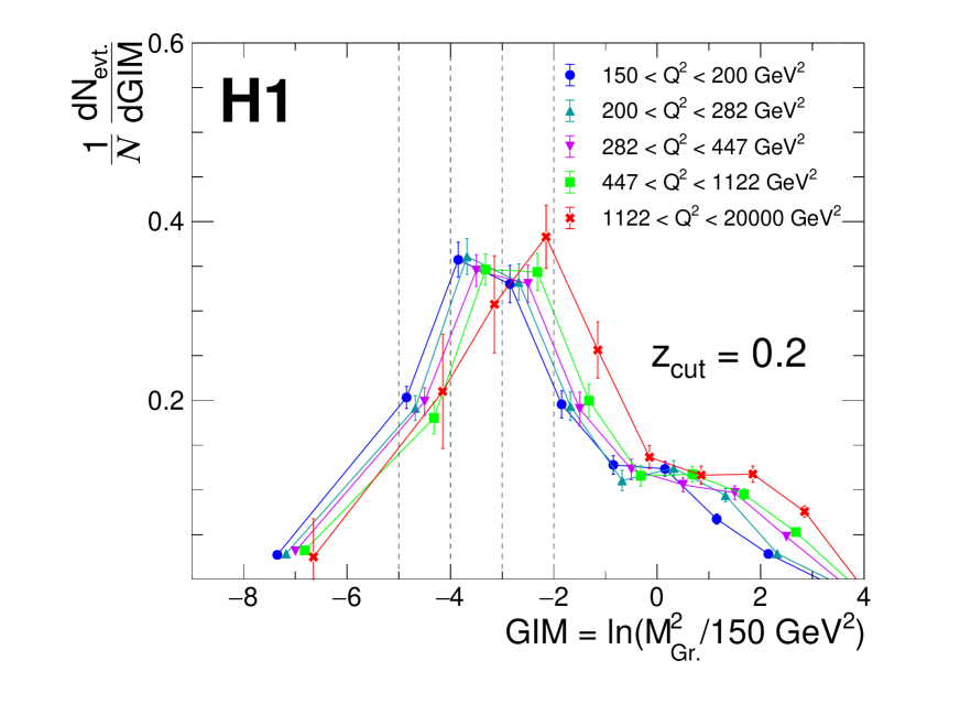
Figure 5: Number of events as a function of GIM for $z_{\mathrm{cut}}$ = 0.2 in several $Q^{2}$ bins, with integral normalized to unity in the region $\mathrm{GIM}<-2$. $Q^{2}_{\mathrm{min.}}$Vertical dotted lines show bin boundaries of bins used in the normalization. The data points are offset horizontally for clarity. The bins have been scaled by their width.

The SCET calculation predicts that the shape of the groomed invariant mass distribution is independent of $Q^{2}$ in the low mass limit, defined by the relation

$$\frac{M^{2}_{\text{Gr.}}}{Q^{2}}\ll z_{\mathrm{cut}}\ll 1.$$ (9)

Figure 5, which tests this prediction, shows the GIM distribution for $z_{\mathrm{cut}}$ = 0.2 in five bins of $Q^{2}$. The factor $Q^{2}_{\mathrm{min.}}$is taken to be 150 $\mathrm{GeV}^{2}$ for all $Q^{2}$ bins. The integrals of all $Q^{2}$ distributions are normalized in the region $\mathrm{GIM}<-2$. In this region, the $x_{\mathrm{Bj}}$ and $Q^{2}$-dependence of the cross section occurs only in the component of the event that has been groomed away; the groomed distribution is therefore expected to be invariant with respect to $x_{\mathrm{Bj}}$ and $Q^{2}$. The shape of the distributions shown in Fig. 5 is observed to be independent of $Q^{2}$, in agreement with this prediction.

7.3 Double-differential cross sections

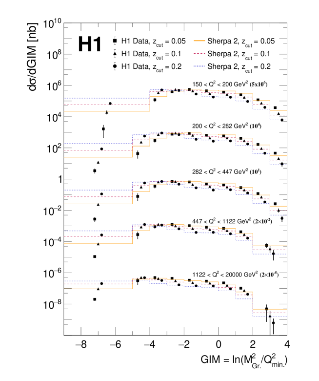
Figure 6: Double-differential groomed invariant mass distributions for $z_{\mathrm{cut}}=0.05$, 0.1, and 0.2, for five bins in $Q^{2}$. The value of $Q^{2}_{\mathrm{min.}}$is taken to be the lowest value of $Q^{2}$ in the bin, e.g. 1122 $\mathrm{GeV}^{2}$ for the highest $Q^{2}$ bin. Uncertainty bars on the data show the quadrature sum of the statistical and systematic uncertainties. The data points are horizontally offset from the bin center for visibility. The lines represent predictions from Sherpa 2 using the cluster hadronization model. The five distributions at different values of $Q^{2}$ are vertically offset by the factor given in parentheses.

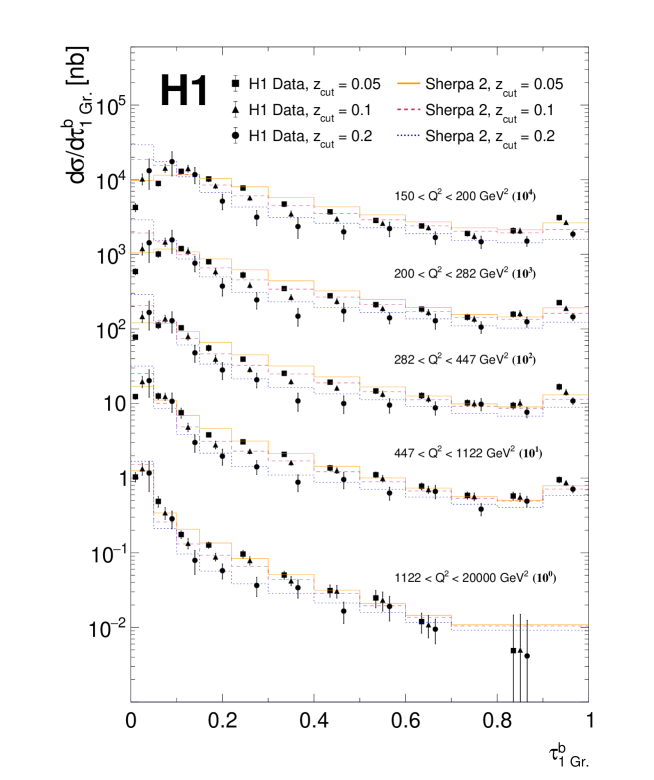
Figure 7: Double-differential $\tau^{b}_{1_{\text{Gr.}}}$ cross section for $z_{\mathrm{cut}}=0.05$, 0.1, and 0.2, presented in five bins in $Q^{2}$. Further details are given in the caption of Fig. 6

Figures 6 and 7 show double-differential cross sections of GIM and $\tau^{b}_{1_{\text{Gr.}}}$, alongside calculations from Sherpa 2 with the cluster hadronization model for comparison. The data are presented in five bins of $Q^{2}$ and at three values of $z_{\mathrm{cut}}$. The binning used in these figures is presented in Tab. 1.

Observable	Binning
Standard $\tau^{b}_{1_{\text{Gr.}}}$	$[0.0,0.05,0.10,0.15,0.22,0.3,0.4,0.5,0.6,0.7,0.8,0.9,1.00]$
Reduced $\tau^{b}_{1_{\text{Gr.}}}$	$[0.0,0.05,0.10,0.15,0.22,0.3,0.4,0.5,0.6,0.7,1.00]$
Standard $\mathrm{ln}(M_{\text{Gr.}}^{2}/Q^{2}_{\mathrm{min.}})$	$[-9,-5,-4,-3,-2,-1,0,1,2,3,4]$
Reduced Low $\mathrm{ln}(M_{\text{Gr.}}^{2}/Q^{2}_{\mathrm{min.}})$	$[-9,-4,-3,-2,-1,0,1,2,3,4]$
Reduced High $\mathrm{ln}(M_{\text{Gr.}}^{2}/Q^{2}_{\mathrm{min.}})$	$[-9,-5,-4,-3,-2,-1,0,1,2,4]$
$Q^{2}$	$[150,200,282,447,1122,20000]$ $\mathrm{GeV}^{2}$

Table 1: Binnings used in the analysis. The reduced binnings are used only in the low-statistics regions of the double-differential result.

Bins with very small event counts were merged with the neighboring bins. The numerical values of the data are provided in tables 8, 9, 10, 11, 12, 13, 14, 15, 16 and 17.

A reasonable agreement between the predictions of Sherpa 2 and the data is found in the majority of bins, with some tension observed at very low $\tau^{b}_{1_{\text{Gr.}}}$ and GIM. The description of the peak region of the $\tau^{b}_{1_{\text{Gr.}}}$ distribution can be seen to improve with $Q^{2}$.

At higher values of $Q^{2}$, the mean values of the event shape distributions decrease, in accordance with the expectation from QCD. These measurements may provide new constraints on the strong coupling constant $\alpha_{\rm s}$.

8 Summary

This paper presents the first measurement of groomed event shape observables in deep inelastic $ep$ collisions. Measurements of the invariant mass and 1-jettiness $\tau^{b}_{1_{\text{Gr.}}}$ of the groomed hadronic final state are reported for $e^{-}p$ collisions at $\sqrt{s}=319$ GeV, for events selected with $Q^{2}>150$ GeV² and $0.2<y<0.7$. Events are clustered using the Centauro jet algorithm, and results are presented for values of the grooming parameter $z_{\mathrm{cut}}=0.05$, 0.1, and 0.2. Cross sections are reported single- and double-differentially.

Event grooming suppresses non-perturbative contributions to event shape distributions in a theoretically well-controlled way. Comparisons of Monte Carlo models and analytical pQCD calculations to these data therefore provide significant new tests of their implementation of both perturbative and non-perturbative processes.

Two of the models that are commonly compared to HERA data, Rapgap and Djangoh, can describe the data in the fixed-order tail regions of the groomed event shape distributions but underestimate the single-jet peak regions. More recently developed models, Pythia 8, Herwig 7, and Sherpa 2, underestimate the fixed-order tail region. The agreement of the models with the data in the low-mass or low-$\tau^{b}_{1_{\text{Gr.}}}$ region improves for higher $z_{\mathrm{cut}}$. Sherpa 3 accurately describes the full distribution of the groomed 1-jettiness within the experimental and theoretical uncertainties.

The numerical predictions of the SCET calculation fail for the lower $z_{\mathrm{cut}}$ values. Comparison of the calculation with data indicates overall a preference for a larger value of the non-perturbative shape function $\Omega_{\mathrm{NP}}$, suggesting that hadronization and other non-perturbative effects are significant in the single-jet limit. The prediction of Ref. [89], that the shape of the low-mass region is independent of the hard scale $Q^{2}$, is found to hold in spite of the disagreement between the numerical predictions and the data.

Event shapes are sensitive to many aspects of QCD final states, making them valuable input for tuning MC event generators. However, such models contain many parameters and determining their optimum values is challenging, since a given effect can often be correctly described by tuning multiple different parameters. The introduction of grooming suppresses the contribution of certain event components, such as the proton beam fragmentation, and causes others, such as the contribution from soft radiation, to scale with $z_{\mathrm{cut}}$.

An accurate description of DIS in MC event generators is crucial for the scientific program of the upcoming Electron-Ion Collider [92]. Future facilities currently under discussion, the LHeC [169, 170] and FCC-eh [171], likewise will require precise MC modeling of the DIS hadronic final state to achieve their physics goals. The groomed event shape distributions reported here provide new, differential constraints for the tuning of MC models and offer the possibility for extracting PDFs and fundamental QCD parameters such as $\alpha_{s}$.

9 Tables

Numerical data are provided for the single-differential cross sections as a function of the groomed invariant mass for grooming parameter $z_{\mathrm{cut}}=0.05$ in Tab. 2, for $z_{\mathrm{cut}}=0.1$ in Tab. 3, and for $z_{\mathrm{cut}}=0.2$ in Tab. 4. Similarly, numerical cross-section data are presented as a function of the groomed 1-jettiness for grooming parameter $z_{\mathrm{cut}}=0.05$ in Tab. 5, for $z_{\mathrm{cut}}=0.1$ in Tab. 6, and for $z_{\mathrm{cut}}=0.2$ in Tab. 7.

1D Groomed invariant mass cross section for $z_{\mathrm{cut}}=0.05$
ln($M^{2}_{Gr.}/150~{}\mathrm{GeV}^{2}$) range		Results	Uncertainty										QED Factor
$\mathrm{Bin~{}Min.}$	$\mathrm{Bin~{}Max.}$	$d\sigma/d\mathrm{GIM}$	Total	Stat.	JES	RCES	$\theta_{\mathrm{HFS}}$	$E_{e}$	$\theta_{e}$	Lumi	Reg.	Model	$c_{\mathrm{QED}}$
		$[\text{pb}]$	[%]	[%]	[%]	[%]	[%]	[%]	[%]	[%]	[%]	[%]
-9	-5	7.09e-01	20.8	16.8	1.6	0.6	-0.0	-0.5	-0.1	2.7	2.3	9.1	1.184
-5	-4	9.02e+00	19.8	9.4	3.6	0.6	-0.1	-1.0	0.2	2.7	2.2	16.2	1.158
-4	-3	7.30e+01	13.1	3.1	3.6	0.7	0.0	-0.8	0.2	2.7	1.6	10.9	1.163
-3	-2	2.47e+02	8.1	1.5	1.0	0.7	0.1	-0.7	0.2	2.7	2.4	5.6	1.160
-2	-1	3.74e+02	7.1	1.2	-0.5	0.5	0.1	-0.8	0.3	2.7	2.5	4.1	1.162
-1	0	2.97e+02	8.8	0.9	1.0	0.3	0.2	-1.4	0.4	2.7	1.6	7.2	1.156
0	1	2.43e+02	7.4	0.9	1.9	-0.7	0.0	-1.7	0.4	2.7	1.4	5.0	1.158
1	2	1.95e+02	6.5	1.2	1.4	-1.3	-0.1	-1.1	0.2	2.7	0.9	4.0	1.157
2	3	1.05e+02	6.1	1.6	0.1	-0.7	-0.3	-0.7	0.2	2.7	0.5	4.0	1.161
3	4	3.39e+01	6.2	3.5	-1.3	-0.3	-0.7	-0.3	0.1	2.7	0.4	2.4	1.171

Table 2: Single-differential groomed invariant mass cross sections for $z_{\mathrm{cut}}=0.05$. The statistical error represents the outcome of the replica method described in Sec. 6. The sources of systematic uncertainty are described in detail in Sec. 6. The total uncertainty on the data is the quadrature sum of the statistical and systematic errors. $c_{\mathrm{QED}}$ is the QED correction factor as derived from HERACLES; the radiative cross section can be recovered by dividing the given data by the corresponding value of $c_{\mathrm{QED}}$.

1D Groomed invariant mass cross section for $z_{\mathrm{cut}}=0.1$
ln($M^{2}_{Gr.}/150~{}\mathrm{GeV}^{2}$) range		Results	Uncertainty										QED Factor
$\mathrm{Bin~{}Min.}$	$\mathrm{Bin~{}Max.}$	$d\sigma/d\mathrm{GIM}$	Total	Stat.	JES	RCES	$\theta_{\mathrm{HFS}}$	$E_{e}$	$\theta_{e}$	Lumi	Reg.	Model	$c_{\mathrm{QED}}$
		$[\text{pb}]$	[%]	[%]	[%]	[%]	[%]	[%]	[%]	[%]	[%]	[%]
-9	-5	3.83e+00	13.6	6.8	2.6	0.3	-0.0	-0.9	0.1	2.7	1.6	9.9	1.167
-5	-4	6.31e+01	11.8	4.3	3.5	0.3	-0.0	-0.9	0.2	2.7	2.0	9.0	1.161
-4	-3	2.22e+02	8.0	1.9	2.5	0.3	-0.0	-0.9	0.2	2.7	1.9	5.0	1.161
-3	-2	3.66e+02	6.1	1.4	-0.0	0.3	0.1	-0.7	0.3	2.7	1.3	3.2	1.160
-2	-1	3.07e+02	6.8	1.3	-0.6	0.4	0.1	-1.0	0.3	2.7	1.0	4.7	1.161
-1	0	1.97e+02	9.6	1.1	1.5	0.0	0.1	-1.7	0.4	2.7	1.1	8.1	1.157
0	1	1.81e+02	7.1	1.2	2.0	-0.9	0.1	-1.7	0.4	2.7	0.8	4.6	1.158
1	2	1.38e+02	6.0	1.5	0.9	-0.9	-0.0	-0.9	0.2	2.7	0.5	3.6	1.157
2	3	6.80e+01	5.8	2.0	-0.5	-0.3	-0.2	-0.4	0.1	2.7	0.4	3.3	1.163
3	4	1.87e+01	6.3	4.2	-1.5	-0.3	-0.6	-0.2	0.1	2.7	0.3	2.3	1.170

Table 3: Same as Table 2 for the GIM cross section at $z_{\mathrm{cut}}=0.1$.

1D Groomed invariant mass cross section for $z_{\mathrm{cut}}=0.2$
ln($M^{2}_{Gr.}/150~{}\mathrm{GeV}^{2}$) range		Results	Uncertainty										QED Factor
$\mathrm{Bin~{}Min.}$	$\mathrm{Bin~{}Max.}$	$d\sigma/d\mathrm{GIM}$	Total	Stat.	JES	RCES	$\theta_{\mathrm{HFS}}$	$E_{e}$	$\theta_{e}$	Lumi	Reg.	Model	$c_{\mathrm{QED}}$
		$[\text{pb}]$	[%]	[%]	[%]	[%]	[%]	[%]	[%]	[%]	[%]	[%]
-9	-5	2.74e+01	7.9	3.7	1.8	0.2	-0.0	-1.1	0.2	2.7	0.6	4.2	1.166
-5	-4	1.89e+02	7.5	2.7	2.4	0.2	-0.0	-1.0	0.2	2.7	0.3	4.2	1.160
-4	-3	3.42e+02	6.1	1.5	1.1	0.1	-0.0	-1.0	0.3	2.7	0.9	2.9	1.161
-3	-2	3.31e+02	6.2	1.4	-0.7	0.0	0.1	-0.9	0.3	2.7	1.3	3.5	1.159
-2	-1	1.95e+02	9.0	1.5	-0.5	0.4	0.1	-1.2	0.3	2.7	1.0	7.6	1.157
-1	0	1.17e+02	9.9	1.4	1.9	-0.1	0.1	-1.9	0.4	2.7	0.7	8.4	1.156
0	1	1.17e+02	7.0	1.6	1.7	-0.8	0.1	-1.7	0.4	2.7	0.5	4.4	1.159
1	2	8.61e+01	6.1	1.9	0.1	-0.7	-0.0	-0.6	0.1	2.7	0.4	3.8	1.158
2	3	3.82e+01	6.1	2.6	-0.7	-0.3	-0.1	-0.2	0.1	2.7	0.3	3.4	1.165
3	4	9.20e+00	7.6	5.5	-1.6	-0.1	-0.4	-0.1	0.1	2.7	0.2	2.8	1.174

Table 4: Same as Table 2 for the GIM cross section at $z_{\mathrm{cut}}=0.2$.

1D $\tau^{b}_{1_{\text{Gr.}}}$ cross section for $z_{\mathrm{cut}}=0.05$
$\tau^{b}_{1_{\text{Gr.}}}$ range		Results	Uncertainty										QED Factor
$\mathrm{Bin~{}Min.}$	$\mathrm{Bin~{}Max.}$	$d\sigma/d\mathrm{\tau^{b}_{1_{\text{Gr.}}}}$	Total	Stat.	JES	RCES	$\theta_{\mathrm{HFS}}$	$E_{e}$	$\theta_{e}$	Lumi	Reg.	Model	$c_{\mathrm{QED}}$
		$[\text{pb}]$	[%]	[%]	[%]	[%]	[%]	[%]	[%]	[%]	[%]	[%]
0.00	0.05	3.77e+03	7.9	0.9	2.0	0.3	0.0	-1.1	0.1	2.7	3.8	4.0	1.181
0.05	0.10	4.88e+03	8.4	0.9	0.8	0.7	0.1	-0.9	0.3	2.7	6.0	3.5	1.156
0.10	0.15	4.39e+03	7.4	1.1	0.2	0.4	0.1	-0.8	0.3	2.7	3.8	4.0	1.157
0.15	0.22	2.94e+03	7.6	1.8	0.8	-0.2	0.1	-1.0	0.3	2.7	5.0	2.8	1.157
0.22	0.30	1.99e+03	7.9	2.3	1.4	-0.2	-0.0	-1.2	0.4	2.7	4.9	2.9	1.157
0.30	0.40	1.37e+03	7.2	2.2	1.5	-0.4	0.0	-1.5	0.4	2.7	3.7	3.1	1.155
0.40	0.50	1.03e+03	6.3	2.8	1.3	-0.6	-0.1	-1.6	0.4	2.7	2.5	1.6	1.153
0.50	0.60	7.84e+02	6.3	3.3	1.2	-0.5	0.0	-1.6	0.4	2.7	1.7	1.2	1.156
0.60	0.70	6.70e+02	6.3	3.8	0.7	-0.6	-0.1	-1.4	0.3	2.7	1.0	1.5	1.155
0.70	0.80	5.23e+02	6.5	4.0	0.2	-0.4	0.1	-1.1	0.4	2.7	0.7	1.4	1.156
0.80	0.90	5.30e+02	6.9	3.5	0.8	-1.2	-0.1	-0.7	0.3	2.7	0.3	3.6	1.155
0.90	1.00	8.18e+02	5.3	1.5	-0.7	-0.1	0.1	0.4	0.1	2.7	0.2	1.9	1.157

Table 5: Same as Table 2 for the $\tau^{b}_{1_{\text{Gr.}}}$ cross section at $z_{\mathrm{cut}}=0.05$.

1D $\tau^{b}_{1_{\text{Gr.}}}$ cross section for $z_{\mathrm{cut}}=0.1$
$\tau^{b}_{1_{\text{Gr.}}}$ range		Results	Uncertainty										QED Factor
$\mathrm{Bin~{}Min.}$	$\mathrm{Bin~{}Max.}$	$d\sigma/d\mathrm{\tau^{b}_{1_{\text{Gr.}}}}$	Total	Stat.	JES	RCES	$\theta_{\mathrm{HFS}}$	$E_{e}$	$\theta_{e}$	Lumi	Reg.	Model	$c_{\mathrm{QED}}$
		$[\text{pb}]$	[%]	[%]	[%]	[%]	[%]	[%]	[%]	[%]	[%]	[%]
0.00	0.05	6.83e+03	6.8	0.6	1.9	0.1	-0.0	-1.0	0.2	2.7	3.2	2.6	1.172
0.05	0.10	5.74e+03	8.6	0.8	0.6	0.4	0.1	-0.8	0.3	2.7	6.5	3.1	1.156
0.10	0.15	3.98e+03	8.4	1.4	-0.4	0.5	0.1	-0.8	0.4	2.7	4.9	4.8	1.155
0.15	0.22	2.09e+03	9.6	2.4	0.8	0.2	0.1	-1.4	0.3	2.7	7.0	3.7	1.158
0.22	0.30	1.50e+03	9.9	3.0	1.5	-0.3	-0.0	-1.4	0.4	2.7	7.0	3.9	1.158
0.30	0.40	1.04e+03	8.5	3.0	1.8	-0.4	0.0	-1.6	0.3	2.7	5.3	3.1	1.155
0.40	0.50	8.66e+02	7.2	3.5	1.3	-0.6	0.0	-1.6	0.5	2.7	3.5	1.9	1.153
0.50	0.60	7.21e+02	7.0	4.1	1.2	-0.4	0.0	-1.6	0.4	2.7	2.3	1.2	1.156
0.60	0.70	6.03e+02	6.8	4.6	0.6	-0.5	-0.1	-1.3	0.3	2.7	1.3	1.2	1.155
0.70	0.80	4.98e+02	6.7	4.2	0.1	-0.3	0.1	-1.0	0.4	2.7	0.8	1.2	1.155
0.80	0.90	5.47e+02	6.3	3.5	0.8	-1.2	-0.1	-0.5	0.2	2.7	0.4	2.2	1.156
0.90	1.00	6.88e+02	5.0	1.6	-0.8	-0.0	0.1	0.4	0.1	2.7	0.3	1.4	1.156

Table 6: Same as Table 2 for the $\tau^{b}_{1_{\text{Gr.}}}$ cross section at $z_{\mathrm{cut}}=0.1$.

1D $\tau^{b}_{1_{\text{Gr.}}}$ cross section for $z_{\mathrm{cut}}=0.2$
$\tau^{b}_{1_{\text{Gr.}}}$ range		Results	Uncertainty										QED Factor
$\mathrm{Bin~{}Min.}$	$\mathrm{Bin~{}Max.}$	$d\sigma/d\mathrm{\tau^{b}_{1_{\text{Gr.}}}}$	Total	Stat.	JES	RCES	$\theta_{\mathrm{HFS}}$	$E_{e}$	$\theta_{e}$	Lumi	Reg.	Model	$c_{\mathrm{QED}}$
		$[\text{pb}]$	[%]	[%]	[%]	[%]	[%]	[%]	[%]	[%]	[%]	[%]
0.00	0.05	1.02e+04	6.2	0.5	1.7	0.1	-0.0	-0.9	0.2	2.7	2.5	2.0	1.168
0.05	0.10	6.10e+03	9.5	0.9	0.5	0.1	0.1	-0.9	0.4	2.7	7.0	4.1	1.156
0.10	0.15	3.34e+03	12.0	1.7	-0.2	0.3	0.1	-1.2	0.4	2.7	9.8	4.9	1.155
0.15	0.22	1.49e+03	8.5	3.1	0.7	0.4	0.1	-1.6	0.4	2.7	5.5	3.3	1.154
0.22	0.30	1.09e+03	9.6	4.2	0.8	0.3	0.1	-1.6	0.4	2.7	4.3	6.0	1.153
0.30	0.40	7.19e+02	9.0	4.3	2.2	-0.5	0.1	-2.0	0.5	2.7	3.8	4.3	1.156
0.40	0.50	6.36e+02	8.0	5.0	1.7	-0.6	0.1	-1.7	0.4	2.7	2.9	2.4	1.157
0.50	0.60	5.92e+02	7.8	5.5	1.0	-0.5	0.0	-1.4	0.4	2.7	1.9	1.7	1.156
0.60	0.70	4.92e+02	7.6	5.7	0.3	-0.5	0.0	-1.0	0.2	2.7	1.1	1.6	1.155
0.70	0.80	4.44e+02	6.9	5.0	-0.1	-0.2	0.1	-0.6	0.3	2.7	0.6	1.2	1.155
0.80	0.90	4.24e+02	6.7	4.2	0.6	-1.2	-0.3	-0.5	0.2	2.7	0.3	2.2	1.157
0.90	1.00	5.28e+02	5.2	1.9	-0.8	0.0	0.2	0.4	0.1	2.7	0.2	1.2	1.157

Table 7: Same as Table 2 for the $\tau^{b}_{1_{\text{Gr.}}}$ cross section at $z_{\mathrm{cut}}=0.2$.

Numerical data on double-differential measurements as a function of the groomed invariant mass, $z_{\mathrm{cut}}$ and $Q^{2}$ are shown in Tab. 8 for $150<Q^{2}<200$ $\mathrm{GeV}^{2}$, Tab. 9 for $200<Q^{2}<282$ $\mathrm{GeV}^{2}$, Tab. 10 for $282<Q^{2}<447$ $\mathrm{GeV}^{2}$, Tab. 11 for $447<Q^{2}<1122$ $\mathrm{GeV}^{2}$, and Tab. 12 for $1122<Q^{2}<20000$ $\mathrm{GeV}^{2}$. Note that $Q^{2}_{\mathrm{min}}$ and hence the definition of the GIM variable is different is different for each $Q^{2}$ interval.

Groomed invariant mass cross section for three values of $z_{\mathrm{cut}}$ and $150<Q^{2}<200$ $\mathrm{GeV}^{2}$
ln($M^{2}_{\mathrm{Gr.}}/Q^{2}_{\mathrm{min.}}$) Range		$z_{\mathrm{cut}}=0.05$				$z_{\mathrm{cut}}=0.1$				$z_{\mathrm{cut}}=0.2$
		$d\sigma/d\mathrm{GIM}$	$\mathrm{Stat.}$	$\mathrm{Sys.}$	$c_{\mathrm{QED}}$	$d\sigma/d\mathrm{GIM}$	$\mathrm{Stat.}$	$\mathrm{Sys.}$	$c_{\mathrm{QED}}$	$d\sigma/d\mathrm{GIM}$	$\mathrm{Stat.}$	$\mathrm{Sy\ s.}$	$c_{\mathrm{QED}}$
$\mathrm{Bin~{}Min.}$	$\mathrm{Bin~{}Max.}$	[pb]	[%]	[%]		[pb]	[%]	[%]		[pb]	[%]	[%]
-9	-4	$2.12\cdot 10^{0}$	16.4	65.3	1.140	$2.07\cdot 10^{1}$	6.0	11.3	1.132	$5.86\cdot 10^{1}$	3.4	6.1	1.131
-4	-3	$2.38\cdot 10^{1}$	4.4	25.1	1.131	$6.83\cdot 10^{1}$	2.0	10.3	1.132	$1.03\cdot 10^{2}$	1.9	6.5	1.133
-3	-2	$7.86\cdot 10^{1}$	1.8	12.0	1.132	$1.09\cdot 10^{2}$	1.4	8.5	1.135	$9.54\cdot 10^{1}$	2.1	7.3	1.136
-2	-1	$1.10\cdot 10^{2}$	1.4	11.5	1.136	$8.95\cdot 10^{1}$	1.6	8.8	1.137	$5.61\cdot 10^{1}$	2.7	8.2	1.135
-1	0	$8.96\cdot 10^{1}$	1.3	7.6	1.132	$6.07\cdot 10^{1}$	1.6	8.6	1.133	$3.60\cdot 10^{1}$	2.6	8.8	1.134
0	1	$7.43\cdot 10^{1}$	1.4	9.1	1.135	$5.34\cdot 10^{1}$	1.9	6.3	1.134	$3.50\cdot 10^{1}$	3.4	6.9	1.136
1	2	$5.08\cdot 10^{1}$	2.3	6.4	1.136	$3.49\cdot 10^{1}$	3.0	6.5	1.135	$1.89\cdot 10^{1}$	4.6	7.9	1.137
2	3	$2.37\cdot 10^{1}$	4.3	8.2	1.136	$1.47\cdot 10^{1}$	5.2	7.0	1.136	$7.86\cdot 10^{0}$	7.4	7.1	1.137
3	4	$7.50\cdot 10^{0}$	9.4	6.6	1.142	$3.20\cdot 10^{0}$	11.8	6.8	1.135	$1.22\cdot 10^{0}$	20.9	7.7	1.142

Table 8: Groomed invariant mass cross section in the range $150<Q^{2}<200$ $\mathrm{GeV}^{2}$. $Q^{2}_{\mathrm{min.}}$ is set to 150 GeV². The statistical error represents the outcome of the replica method described in Sec. 6. The systematic uncertainty is the quadrature sum of all the sources listed in Sec. 6. The total uncertainty on the data is the quadrature sum of the statistical and systematic errors given here. $c_{\mathrm{QED}}$ is the QED correction factor as derived from HERACLES; the radiative cross section can be recovered by dividing the given data by the corresponding value of $c_{\mathrm{QED}}$. The lowest bins in groomed invariant mass were consolidated due to low statistics. The binning follows the reduced low GIM binning given in Table 1.

Groomed invariant mass cross section for three values of $z_{\mathrm{cut}}$ and $200<Q^{2}<282$ $\mathrm{GeV}^{2}$
ln($M^{2}_{\mathrm{Gr.}}/Q^{2}_{\mathrm{min.}}$) Range		$z_{\mathrm{cut}}=0.05$				$z_{\mathrm{cut}}=0.1$				$z_{\mathrm{cut}}=0.2$
		$d\sigma/d\mathrm{GIM}$	$\mathrm{Stat.}$	$\mathrm{Sys.}$	$c_{\mathrm{QED}}$	$d\sigma/d\mathrm{GIM}$	$\mathrm{Stat.}$	$\mathrm{Sys.}$	$c_{\mathrm{QED}}$	$d\sigma/d\mathrm{GIM}$	$\mathrm{Stat.}$	$\mathrm{Sy\ s.}$	$c_{\mathrm{QED}}$
$\mathrm{Bin~{}Min.}$	$\mathrm{Bin~{}Max.}$	[pb]	[%]	[%]		[pb]	[%]	[%]		[pb]	[%]	[%]
-9	-5	$3.46\cdot 10^{-1}$	29.6	9.6	1.135	$1.20\cdot 10^{0}$	9.7	15.0	1.130	$8.58\cdot 10^{0}$	4.6	9.5	1.132
-5	-4	$4.32\cdot 10^{0}$	12.3	49.4	1.125	$2.34\cdot 10^{1}$	4.7	11.4	1.133	$5.70\cdot 10^{1}$	3.2	6.4	1.131
-4	-3	$2.97\cdot 10^{1}$	3.7	23.0	1.133	$7.14\cdot 10^{1}$	1.9	7.6	1.131	$8.99\cdot 10^{1}$	2.1	6.7	1.134
-3	-2	$7.59\cdot 10^{1}$	1.7	9.9	1.132	$8.84\cdot 10^{1}$	1.7	7.6	1.132	$7.10\cdot 10^{1}$	2.7	7.0	1.134
-2	-1	$8.50\cdot 10^{1}$	1.6	10.2	1.133	$6.38\cdot 10^{1}$	1.9	8.8	1.137	$3.54\cdot 10^{1}$	3.0	10.6	1.134
-1	0	$6.46\cdot 10^{1}$	1.4	10.2	1.135	$4.33\cdot 10^{1}$	1.7	9.9	1.135	$2.68\cdot 10^{1}$	3.0	9.1	1.135
0	1	$5.92\cdot 10^{1}$	1.7	5.8	1.134	$4.40\cdot 10^{1}$	2.2	7.3	1.134	$2.78\cdot 10^{1}$	3.8	7.3	1.135
1	2	$4.11\cdot 10^{1}$	2.8	7.9	1.136	$2.86\cdot 10^{1}$	3.6	7.3	1.137	$1.77\cdot 10^{1}$	5.3	7.4	1.139
2	3	$1.65\cdot 10^{1}$	5.0	7.2	1.137	$9.11\cdot 10^{0}$	6.2	6.8	1.140	$4.55\cdot 10^{0}$	8.2	7.4	1.139
3	4	$4.59\cdot 10^{0}$	11.0	6.8	1.140	$2.09\cdot 10^{0}$	14.3	10.6	1.136	$9.37\cdot 10^{-1}$	25.4	14.9	1.137

Table 9: Same as Table 8 for groomed invariant mass cross sections in the range $200<Q^{2}<282$ $\mathrm{GeV}^{2}$. $Q^{2}_{\mathrm{min.}}$ is set to 200 GeV². The binning follows the standard GIM binning given in Table 1.

Groomed invariant mass cross section for three values of $z_{\mathrm{cut}}$ and $282<Q^{2}<447$ $\mathrm{GeV}^{2}$
ln($M^{2}_{\mathrm{Gr.}}/Q^{2}_{\mathrm{min.}}$) Range		$z_{\mathrm{cut}}=0.05$				$z_{\mathrm{cut}}=0.1$				$z_{\mathrm{cut}}=0.2$
		$d\sigma/d\mathrm{GIM}$	$\mathrm{Stat.}$	$\mathrm{Sys.}$	$c_{\mathrm{QED}}$	$d\sigma/d\mathrm{GIM}$	$\mathrm{Stat.}$	$\mathrm{Sys.}$	$c_{\mathrm{QED}}$	$d\sigma/d\mathrm{GIM}$	$\mathrm{Stat.}$	$\mathrm{Sy\ s.}$	$c_{\mathrm{QED}}$
$\mathrm{Bin~{}Min.}$	$\mathrm{Bin~{}Max.}$	[pb]	[%]	[%]		[pb]	[%]	[%]		[pb]	[%]	[%]
-9	-5	$2.75\cdot 10^{-1}$	18.3	26.3	1.134	$2.39\cdot 10^{0}$	7.4	10.5	1.134	$1.12\cdot 10^{1}$	3.6	6.7	1.136
-5	-4	$7.86\cdot 10^{0}$	8.8	47.9	1.137	$3.09\cdot 10^{1}$	3.8	11.1	1.136	$5.66\cdot 10^{1}$	3.0	6.0	1.137
-4	-3	$3.52\cdot 10^{1}$	3.1	23.8	1.137	$6.59\cdot 10^{1}$	2.1	7.5	1.135	$7.05\cdot 10^{1}$	2.5	6.3	1.134
-3	-2	$7.06\cdot 10^{1}$	2.0	10.3	1.134	$6.86\cdot 10^{1}$	2.0	8.2	1.135	$4.71\cdot 10^{1}$	3.3	8.3	1.135
-2	-1	$6.64\cdot 10^{1}$	1.7	10.1	1.135	$4.49\cdot 10^{1}$	2.1	9.6	1.136	$2.76\cdot 10^{1}$	3.3	10.3	1.137
-1	0	$4.89\cdot 10^{1}$	1.7	9.4	1.137	$3.39\cdot 10^{1}$	2.2	8.0	1.137	$1.98\cdot 10^{1}$	3.4	8.3	1.138
0	1	$4.28\cdot 10^{1}$	2.2	6.4	1.138	$3.14\cdot 10^{1}$	2.9	7.2	1.137	$2.09\cdot 10^{1}$	4.6	7.3	1.137
1	2	$2.85\cdot 10^{1}$	3.5	7.5	1.136	$2.01\cdot 10^{1}$	4.3	7.0	1.138	$1.29\cdot 10^{1}$	6.5	7.3	1.140
2	3	$1.19\cdot 10^{1}$	6.1	6.1	1.141	$7.11\cdot 10^{0}$	7.9	5.4	1.141	$3.45\cdot 10^{0}$	10.8	5.9	1.135
3	4	$2.64\cdot 10^{0}$	15.7	8.9	1.157	$1.02\cdot 10^{0}$	23.0	9.9	1.150	$3.07\cdot 10^{-1}$	36.3	14.8	1.148

Table 10: Same as Table 8 for groomed invariant mass cross sections in the range $282<Q^{2}<447$ $\mathrm{GeV}^{2}$. $Q^{2}_{\mathrm{min.}}$ is set to 282 GeV². The binning follows the standard GIM binning given in Table 1.

Groomed invariant mass cross section for three values of $z_{\mathrm{cut}}$ and $447<Q^{2}<1122$ $\mathrm{GeV}^{2}$
ln($M^{2}_{\mathrm{Gr.}}/Q^{2}_{\mathrm{min.}}$) Range		$z_{\mathrm{cut}}=0.05$				$z_{\mathrm{cut}}=0.1$				$z_{\mathrm{cut}}=0.2$
		$d\sigma/d\mathrm{GIM}$	$\mathrm{Stat.}$	$\mathrm{Sys.}$	$c_{\mathrm{QED}}$	$d\sigma/d\mathrm{GIM}$	$\mathrm{Stat.}$	$\mathrm{Sys.}$	$c_{\mathrm{QED}}$	$d\sigma/d\mathrm{GIM}$	$\mathrm{Stat.}$	$\mathrm{Sy\ s.}$	$c_{\mathrm{QED}}$
$\mathrm{Bin~{}Min.}$	$\mathrm{Bin~{}Max.}$	[pb]	[%]	[%]		[pb]	[%]	[%]		[pb]	[%]	[%]
-9	-5	$5.48\cdot 10^{-1}$	11.6	11.6	1.141	$3.54\cdot 10^{0}$	4.8	13.7	1.145	$1.33\cdot 10^{1}$	2.7	9.3	1.142
-5	-4	$1.41\cdot 10^{1}$	5.5	46.4	1.144	$4.29\cdot 10^{1}$	2.9	10.7	1.142	$6.21\cdot 10^{1}$	3.1	5.0	1.141
-4	-3	$4.54\cdot 10^{1}$	2.7	21.9	1.140	$6.31\cdot 10^{1}$	2.2	5.9	1.141	$5.71\cdot 10^{1}$	3.3	5.3	1.142
-3	-2	$6.21\cdot 10^{1}$	2.1	9.7	1.143	$5.05\cdot 10^{1}$	2.5	7.0	1.144	$3.28\cdot 10^{1}$	3.8	9.1	1.140
-2	-1	$5.21\cdot 10^{1}$	1.9	9.8	1.142	$3.44\cdot 10^{1}$	2.3	9.4	1.142	$1.93\cdot 10^{1}$	3.5	9.0	1.143
-1	0	$4.14\cdot 10^{1}$	1.9	6.9	1.145	$3.00\cdot 10^{1}$	2.5	6.2	1.145	$1.95\cdot 10^{1}$	3.6	6.4	1.147
0	1	$3.48\cdot 10^{1}$	2.5	5.2	1.144	$2.52\cdot 10^{1}$	3.0	5.8	1.143	$1.58\cdot 10^{1}$	4.5	6.0	1.144
1	2	$2.13\cdot 10^{1}$	3.6	5.4	1.143	$1.42\cdot 10^{1}$	4.4	4.7	1.144	$8.26\cdot 10^{0}$	6.3	5.1	1.147
2	4	$7.02\cdot 10^{0}$	6.5	3.6	1.150	$4.52\cdot 10^{0}$	8.3	4.6	1.149	$2.21\cdot 10^{0}$	11.8	6.2	1.147

Table 11: Same as Table 8 for groomed invariant mass cross sections in the range $447<Q^{2}<1122$ $\mathrm{GeV}^{2}$. $Q^{2}_{\mathrm{min.}}$ is set to 447 GeV². The binning follows the reduced high GIM binning given in Table 1.

Groomed invariant mass cross section for three values of $z_{\mathrm{cut}}$ and $1122<Q^{2}<20000$ $\mathrm{GeV}^{2}$
ln($M^{2}_{\mathrm{Gr.}}/Q^{2}_{\mathrm{min.}}$) Range		$z_{\mathrm{cut}}=0.05$				$z_{\mathrm{cut}}=0.1$				$z_{\mathrm{cut}}=0.2$
		$d\sigma/d\mathrm{GIM}$	$\mathrm{Stat.}$	$\mathrm{Sys.}$	$c_{\mathrm{QED}}$	$d\sigma/d\mathrm{GIM}$	$\mathrm{Stat.}$	$\mathrm{Sys.}$	$c_{\mathrm{QED}}$	$d\sigma/d\mathrm{GIM}$	$\mathrm{Stat.}$	$\mathrm{Sy\ s.}$	$c_{\mathrm{QED}}$
$\mathrm{Bin~{}Min.}$	$\mathrm{Bin~{}Max.}$	[pb]	[%]	[%]		[pb]	[%]	[%]		[pb]	[%]	[%]
-9	-5	$1.01\cdot 10^{0}$	8.8	15.8	1.210	$4.70\cdot 10^{0}$	4.6	16.7	1.207	$1.03\cdot 10^{1}$	4.0	12.3	1.197
-5	-4	$1.58\cdot 10^{1}$	6.1	45.3	1.210	$2.50\cdot 10^{1}$	5.2	12.8	1.210	$2.44\cdot 10^{1}$	6.7	7.4	1.209
-4	-3	$2.45\cdot 10^{1}$	4.8	20.8	1.210	$2.13\cdot 10^{1}$	4.7	10.1	1.210	$1.64\cdot 10^{1}$	6.3	12.1	1.211
-3	-2	$2.21\cdot 10^{1}$	3.6	14.6	1.216	$1.54\cdot 10^{1}$	3.9	10.5	1.214	$8.47\cdot 10^{0}$	5.6	8.4	1.210
-2	-1	$1.69\cdot 10^{1}$	3.7	8.9	1.205	$1.18\cdot 10^{1}$	4.2	7.0	1.204	$7.33\cdot 10^{0}$	5.2	6.9	1.204
-1	0	$1.47\cdot 10^{1}$	3.7	6.3	1.199	$1.10\cdot 10^{1}$	4.4	6.5	1.200	$7.21\cdot 10^{0}$	5.5	6.6	1.201
0	1	$1.13\cdot 10^{1}$	4.4	5.1	1.204	$7.91\cdot 10^{0}$	5.0	5.9	1.205	$4.71\cdot 10^{0}$	6.9	5.6	1.205
1	2	$5.20\cdot 10^{0}$	7.3	4.1	1.221	$3.68\cdot 10^{0}$	9.1	4.2	1.224	$2.11\cdot 10^{0}$	13.5	5.2	1.231
2	4	$7.65\cdot 10^{-1}$	34.8	8.4	1.250	$2.68\cdot 10^{-1}$	42.7	92.3	1.246	$9.70\cdot 10^{-2}$	47.7	52.2	1.247

Table 12: Same as Table 8 for groomed invariant mass cross sections in the range $1122<Q^{2}<20000$ $\mathrm{GeV}^{2}$. $Q^{2}_{\mathrm{min.}}$ is set to 1122 GeV². The binning follows the reduced high GIM binning given in Table 1.

Groomed $\tau^{b}_{1_{\text{Gr.}}}$ cross section for three values of $z_{\mathrm{cut}}$ and $150<Q^{2}<200$ $\mathrm{GeV}^{2}$
$\tau^{b}_{1_{\text{Gr.}}}$ Range		$z_{\mathrm{cut}}=0.05$				$z_{\mathrm{cut}}=0.1$				$z_{\mathrm{cut}}=0.2$
		$d\sigma/d\tau^{b}_{1_{\text{Gr.}}}$	$\mathrm{Stat.}$	$\mathrm{Sys.}$	$c_{\mathrm{QED}}$	$d\sigma/d\tau^{b}_{1_{\text{Gr.}}}$	$\mathrm{Stat.}$	$\mathrm{Sys.}$	$c_{\mathrm{QED}}$	$d\sigma/d\mathrm{GIM}$	$\mathrm{Stat.}$	$\mathrm{Sy\ s.}$	$c_{\mathrm{QED}}$
$\mathrm{Bin~{}Min.}$	$\mathrm{Bin~{}Max.}$	[pb]	[%]	[%]		[pb]	[%]	[%]		[pb]	[%]	[%]
0.00	0.05	$4.04\cdot 10^{2}$	5.6	8.0	1.137	$1.17\cdot 10^{3}$	3.0	7.1	1.133	$2.26\cdot 10^{3}$	2.8	12.3	1.134
0.05	0.10	$9.47\cdot 10^{2}$	2.9	8.0	1.128	$1.52\cdot 10^{3}$	2.5	7.0	1.133	$2.11\cdot 10^{3}$	2.9	10.6	1.134
0.10	0.15	$1.26\cdot 10^{3}$	2.2	6.5	1.134	$1.37\cdot 10^{3}$	3.1	7.7	1.132	$1.32\cdot 10^{3}$	4.0	9.2	1.134
0.15	0.22	$1.09\cdot 10^{3}$	2.2	6.8	1.136	$9.00\cdot 10^{2}$	3.6	7.0	1.137	$6.53\cdot 10^{2}$	4.9	8.5	1.134
0.22	0.30	$7.38\cdot 10^{2}$	2.3	6.3	1.134	$5.67\cdot 10^{2}$	3.8	6.8	1.136	$3.81\cdot 10^{2}$	5.7	9.3	1.134
0.30	0.40	$4.82\cdot 10^{2}$	2.0	7.2	1.134	$3.61\cdot 10^{2}$	3.1	8.0	1.135	$3.12\cdot 10^{2}$	5.5	15.9	1.135
0.40	0.50	$3.63\cdot 10^{2}$	2.4	7.0	1.135	$2.94\cdot 10^{2}$	3.9	7.5	1.134	$2.32\cdot 10^{2}$	6.5	13.5	1.137
0.50	0.60	$2.83\cdot 10^{2}$	3.3	6.3	1.134	$2.64\cdot 10^{2}$	4.8	5.9	1.133	$2.49\cdot 10^{2}$	7.7	13.2	1.135
0.60	0.70	$2.40\cdot 10^{2}$	4.1	5.6	1.134	$2.30\cdot 10^{2}$	5.8	5.3	1.134	$1.95\cdot 10^{2}$	8.6	7.8	1.133
0.70	0.80	$1.89\cdot 10^{2}$	4.8	5.8	1.133	$1.76\cdot 10^{2}$	6.5	6.9	1.132	$1.65\cdot 10^{2}$	8.4	7.7	1.133
0.80	0.90	$1.98\cdot 10^{2}$	5.3	6.3	1.139	$2.05\cdot 10^{2}$	5.7	6.8	1.139	$1.57\cdot 10^{2}$	7.5	6.9	1.141
0.90	1.00	$3.17\cdot 10^{2}$	2.7	5.8	1.136	$2.66\cdot 10^{2}$	3.2	6.1	1.136	$1.93\cdot 10^{2}$	3.7	5.5	1.136

Table 13: Same as Table 8 for $\tau^{b}_{1_{\text{Gr.}}}$ cross sections in the range $150<Q^{2}<200$ $\mathrm{GeV}^{2}$. The binning follows the standard $\tau^{b}_{1_{\text{Gr.}}}$ binning given in Table 1.

Groomed $\tau^{b}_{1_{\text{Gr.}}}$ cross section for three values of $z_{\mathrm{cut}}$ and $200<Q^{2}<282$ $\mathrm{GeV}^{2}$
$\tau^{b}_{1_{\text{Gr.}}}$ Range		$z_{\mathrm{cut}}=0.05$				$z_{\mathrm{cut}}=0.1$				$z_{\mathrm{cut}}=0.2$
		$d\sigma/d\tau^{b}_{1_{\text{Gr.}}}$	$\mathrm{Stat.}$	$\mathrm{Sys.}$	$c_{\mathrm{QED}}$	$d\sigma/d\tau^{b}_{1_{\text{Gr.}}}$	$\mathrm{Stat.}$	$\mathrm{Sys.}$	$c_{\mathrm{QED}}$	$d\sigma/d\mathrm{GIM}$	$\mathrm{Stat.}$	$\mathrm{Sy\ s.}$	$c_{\mathrm{QED}}$
$\mathrm{Bin~{}Min.}$	$\mathrm{Bin~{}Max.}$	[pb]	[%]	[%]		[pb]	[%]	[%]		[pb]	[%]	[%]
0.00	0.05	$5.73\cdot 10^{2}$	3.3	7.4	1.132	$1.40\cdot 10^{3}$	2.3	5.4	1.130	$2.46\cdot 10^{3}$	2.3	12.3	1.131
0.05	0.10	$1.08\cdot 10^{3}$	2.2	6.5	1.132	$1.50\cdot 10^{3}$	2.5	6.5	1.134	$1.81\cdot 10^{3}$	2.9	11.1	1.133
0.10	0.15	$1.15\cdot 10^{3}$	2.6	7.0	1.132	$1.07\cdot 10^{3}$	3.9	6.6	1.132	$9.09\cdot 10^{2}$	5.2	8.7	1.135
0.15	0.22	$8.16\cdot 10^{2}$	2.7	6.2	1.134	$6.39\cdot 10^{2}$	4.1	7.0	1.134	$4.69\cdot 10^{2}$	5.7	9.8	1.133
0.22	0.30	$5.02\cdot 10^{2}$	2.5	7.6	1.136	$3.87\cdot 10^{2}$	4.1	8.7	1.138	$2.93\cdot 10^{2}$	6.9	11.7	1.136
0.30	0.40	$3.58\cdot 10^{2}$	2.4	6.7	1.135	$2.74\cdot 10^{2}$	3.7	7.2	1.134	$2.06\cdot 10^{2}$	7.2	9.7	1.136
0.40	0.50	$2.73\cdot 10^{2}$	3.2	6.7	1.131	$2.33\cdot 10^{2}$	4.9	7.4	1.131	$1.96\cdot 10^{2}$	7.9	13.6	1.134
0.50	0.60	$2.12\cdot 10^{2}$	4.1	6.8	1.136	$1.90\cdot 10^{2}$	6.0	6.7	1.137	$1.60\cdot 10^{2}$	9.2	8.8	1.134
0.60	0.70	$1.83\cdot 10^{2}$	5.6	6.4	1.137	$1.66\cdot 10^{2}$	7.4	6.3	1.138	$1.47\cdot 10^{2}$	10.4	11.4	1.138
0.70	0.80	$1.44\cdot 10^{2}$	6.3	6.7	1.134	$1.37\cdot 10^{2}$	7.8	6.2	1.135	$1.20\cdot 10^{2}$	10.3	6.2	1.136
0.80	0.90	$1.56\cdot 10^{2}$	6.8	7.0	1.136	$1.62\cdot 10^{2}$	7.0	6.8	1.136	$1.29\cdot 10^{2}$	8.6	7.2	1.135
0.90	1.00	$2.22\cdot 10^{2}$	3.3	5.3	1.139	$1.86\cdot 10^{2}$	3.7	5.5	1.139	$1.49\cdot 10^{2}$	4.4	5.7	1.138

Table 14: Same as Table 8 for $\tau^{b}_{1_{\text{Gr.}}}$ cross sections in the range $200<Q^{2}<282$ $\mathrm{GeV}^{2}$. The binning follows the standard $\tau^{b}_{1_{\text{Gr.}}}$ binning given in Table 1.

Groomed $\tau^{b}_{1_{\text{Gr.}}}$ cross section for three values of $z_{\mathrm{cut}}$ and $282<Q^{2}<447$ $\mathrm{GeV}^{2}$
$\tau^{b}_{1_{\text{Gr.}}}$ Range		$z_{\mathrm{cut}}=0.05$				$z_{\mathrm{cut}}=0.1$				$z_{\mathrm{cut}}=0.2$
		$d\sigma/d\tau^{b}_{1_{\text{Gr.}}}$	$\mathrm{Stat.}$	$\mathrm{Sys.}$	$c_{\mathrm{QED}}$	$d\sigma/d\tau^{b}_{1_{\text{Gr.}}}$	$\mathrm{Stat.}$	$\mathrm{Sys.}$	$c_{\mathrm{QED}}$	$d\sigma/d\mathrm{GIM}$	$\mathrm{Stat.}$	$\mathrm{Sy\ s.}$	$c_{\mathrm{QED}}$
$\mathrm{Bin~{}Min.}$	$\mathrm{Bin~{}Max.}$	[pb]	[%]	[%]		[pb]	[%]	[%]		[pb]	[%]	[%]
0.00	0.05	$7.86\cdot 10^{2}$	2.3	8.5	1.136	$1.70\cdot 10^{3}$	1.8	5.4	1.134	$2.68\cdot 10^{3}$	2.2	11.4	1.135
0.05	0.10	$1.17\cdot 10^{3}$	2.3	6.0	1.134	$1.34\cdot 10^{3}$	2.9	5.8	1.135	$1.45\cdot 10^{3}$	3.5	10.9	1.137
0.10	0.15	$9.89\cdot 10^{2}$	3.4	7.0	1.133	$7.91\cdot 10^{2}$	4.9	6.6	1.137	$6.00\cdot 10^{2}$	6.0	9.0	1.137
0.15	0.22	$5.68\cdot 10^{2}$	2.9	8.6	1.135	$4.29\cdot 10^{2}$	4.7	8.3	1.139	$3.34\cdot 10^{2}$	7.0	10.0	1.137
0.22	0.30	$3.84\cdot 10^{2}$	2.7	7.0	1.137	$2.86\cdot 10^{2}$	4.8	6.7	1.137	$2.43\cdot 10^{2}$	7.9	9.7	1.135
0.30	0.40	$2.59\cdot 10^{2}$	2.9	6.0	1.139	$2.03\cdot 10^{2}$	4.7	6.4	1.138	$1.44\cdot 10^{2}$	8.2	9.4	1.134
0.40	0.50	$1.89\cdot 10^{2}$	4.3	6.5	1.138	$1.60\cdot 10^{2}$	5.7	6.5	1.137	$1.17\cdot 10^{2}$	9.9	11.2	1.143
0.50	0.60	$1.48\cdot 10^{2}$	5.8	6.3	1.138	$1.36\cdot 10^{2}$	7.4	6.6	1.138	$1.10\cdot 10^{2}$	11.0	10.7	1.139
0.60	0.70	$1.28\cdot 10^{2}$	7.4	6.2	1.139	$1.16\cdot 10^{2}$	9.3	5.6	1.139	$9.86\cdot 10^{1}$	11.6	8.7	1.138
0.70	0.80	$1.02\cdot 10^{2}$	8.6	5.5	1.139	$1.00\cdot 10^{2}$	9.6	5.7	1.137	$1.08\cdot 10^{2}$	11.9	7.2	1.137
0.80	0.90	$9.47\cdot 10^{1}$	8.7	6.6	1.135	$1.02\cdot 10^{2}$	8.9	6.2	1.136	$8.05\cdot 10^{1}$	10.6	6.4	1.135
0.90	1.00	$1.59\cdot 10^{2}$	3.9	5.2	1.138	$1.37\cdot 10^{2}$	4.3	5.3	1.138	$1.10\cdot 10^{2}$	5.1	5.0	1.143

Table 15: Same as Table 8 for $\tau^{b}_{1_{\text{Gr.}}}$ cross sections in the range $282<Q^{2}<447$ $\mathrm{GeV}^{2}$. The binning follows the standard $\tau^{b}_{1_{\text{Gr.}}}$ binning given in Table 1.

Groomed $\tau^{b}_{1_{\text{Gr.}}}$ cross section for three values of $z_{\mathrm{cut}}$ and $447<Q^{2}<1122$ $\mathrm{GeV}^{2}$
$\tau^{b}_{1_{\text{Gr.}}}$ Range		$z_{\mathrm{cut}}=0.05$				$z_{\mathrm{cut}}=0.1$				$z_{\mathrm{cut}}=0.2$
		$d\sigma/d\tau^{b}_{1_{\text{Gr.}}}$	$\mathrm{Stat.}$	$\mathrm{Sys.}$	$c_{\mathrm{QED}}$	$d\sigma/d\tau^{b}_{1_{\text{Gr.}}}$	$\mathrm{Stat.}$	$\mathrm{Sys.}$	$c_{\mathrm{QED}}$	$d\sigma/d\mathrm{GIM}$	$\mathrm{Stat.}$	$\mathrm{Sy\ s.}$	$c_{\mathrm{QED}}$
$\mathrm{Bin~{}Min.}$	$\mathrm{Bin~{}Max.}$	[pb]	[%]	[%]		[pb]	[%]	[%]		[pb]	[%]	[%]
0.00	0.05	$1.35\cdot 10^{3}$	1.6	8.4	1.143	$2.26\cdot 10^{3}$	1.5	5.4	1.143	$3.15\cdot 10^{3}$	2.1	11.0	1.142
0.05	0.10	$1.20\cdot 10^{3}$	2.6	10.6	1.142	$1.16\cdot 10^{3}$	3.3	7.5	1.141	$1.16\cdot 10^{3}$	3.6	12.1	1.140
0.10	0.15	$7.32\cdot 10^{2}$	3.3	10.5	1.144	$5.15\cdot 10^{2}$	5.1	11.1	1.144	$3.78\cdot 10^{2}$	7.7	6.9	1.145
0.15	0.22	$3.95\cdot 10^{2}$	3.1	6.3	1.140	$2.90\cdot 10^{2}$	5.3	7.2	1.141	$2.24\cdot 10^{2}$	7.5	10.0	1.143
0.22	0.30	$2.99\cdot 10^{2}$	3.5	6.1	1.143	$2.34\cdot 10^{2}$	5.9	6.1	1.141	$1.64\cdot 10^{2}$	8.9	8.7	1.141
0.30	0.40	$2.12\cdot 10^{2}$	4.0	5.6	1.143	$1.64\cdot 10^{2}$	6.0	6.0	1.144	$1.12\cdot 10^{2}$	9.0	8.2	1.143
0.40	0.50	$1.34\cdot 10^{2}$	5.9	6.0	1.145	$1.26\cdot 10^{2}$	7.1	5.9	1.145	$1.06\cdot 10^{2}$	10.7	11.1	1.148
0.50	0.60	$1.12\cdot 10^{2}$	7.5	5.9	1.148	$9.96\cdot 10^{1}$	9.3	5.4	1.147	$7.10\cdot 10^{1}$	12.6	8.7	1.148
0.60	0.70	$7.74\cdot 10^{1}$	9.7	5.7	1.144	$7.04\cdot 10^{1}$	11.0	4.9	1.145	$7.13\cdot 10^{1}$	13.7	9.6	1.145
0.70	0.80	$5.83\cdot 10^{1}$	10.6	5.0	1.144	$5.64\cdot 10^{1}$	11.5	5.3	1.144	$4.26\cdot 10^{1}$	13.8	6.2	1.143
0.80	0.90	$5.82\cdot 10^{1}$	11.5	6.3	1.146	$5.65\cdot 10^{1}$	11.9	6.1	1.146	$5.04\cdot 10^{1}$	12.6	6.8	1.149
0.90	1.00	$9.20\cdot 10^{1}$	4.9	4.8	1.149	$8.53\cdot 10^{1}$	5.2	5.1	1.155	$7.24\cdot 10^{1}$	5.5	5.5	1.176

Table 16: Same as Table 8 for $\tau^{b}_{1_{\text{Gr.}}}$ cross sections in the range $447<Q^{2}<1122$ $\mathrm{GeV}^{2}$. The binning follows the standard $\tau^{b}_{1_{\text{Gr.}}}$ binning given in Table 1.

Groomed $\tau^{b}_{1_{\text{Gr.}}}$ cross section for three values of $z_{\mathrm{cut}}$ and $1122<Q^{2}<20000$ $\mathrm{GeV}^{2}$
$\tau^{b}_{1_{\text{Gr.}}}$ Range		$z_{\mathrm{cut}}=0.05$				$z_{\mathrm{cut}}=0.1$				$z_{\mathrm{cut}}=0.2$
		$d\sigma/d\tau^{b}_{1_{\text{Gr.}}}$	$\mathrm{Stat.}$	$\mathrm{Sys.}$	$c_{\mathrm{QED}}$	$d\sigma/d\tau^{b}_{1_{\text{Gr.}}}$	$\mathrm{Stat.}$	$\mathrm{Sys.}$	$c_{\mathrm{QED}}$	$d\sigma/d\mathrm{GIM}$	$\mathrm{Stat.}$	$\mathrm{Sy\ s.}$	$c_{\mathrm{QED}}$
$\mathrm{Bin~{}Min.}$	$\mathrm{Bin~{}Max.}$	[pb]	[%]	[%]		[pb]	[%]	[%]		[pb]	[%]	[%]
0.00	0.05	$1.10\cdot 10^{3}$	1.5	8.1	1.223	$1.48\cdot 10^{3}$	1.6	8.2	1.220	$1.84\cdot 10^{3}$	2.4	12.6	1.217
0.05	0.10	$4.47\cdot 10^{2}$	4.0	14.3	1.206	$3.28\cdot 10^{2}$	4.4	14.0	1.200	$2.94\cdot 10^{2}$	5.1	13.4	1.192
0.10	0.15	$1.88\cdot 10^{2}$	7.4	12.8	1.199	$1.44\cdot 10^{2}$	10.2	6.0	1.198	$9.94\cdot 10^{1}$	14.8	10.6	1.188
0.15	0.22	$1.25\cdot 10^{2}$	7.6	6.4	1.194	$8.96\cdot 10^{1}$	9.2	7.2	1.199	$6.28\cdot 10^{1}$	14.2	7.7	1.201
0.22	0.30	$9.64\cdot 10^{1}$	9.7	6.4	1.188	$7.93\cdot 10^{1}$	11.9	6.1	1.191	$4.42\cdot 10^{1}$	18.9	9.3	1.190
0.30	0.40	$5.01\cdot 10^{1}$	12.0	5.3	1.188	$4.25\cdot 10^{1}$	13.5	6.0	1.188	$3.90\cdot 10^{1}$	20.3	7.9	1.188
0.40	0.50	$3.12\cdot 10^{1}$	18.2	5.7	1.177	$3.04\cdot 10^{1}$	21.1	5.3	1.175	$1.73\cdot 10^{1}$	25.6	9.2	1.180
0.50	0.60	$2.47\cdot 10^{1}$	28.9	6.3	1.184	$2.34\cdot 10^{1}$	30.3	6.5	1.184	$2.17\cdot 10^{1}$	34.4	9.6	1.181
0.60	0.70	$1.19\cdot 10^{1}$	33.1	5.6	1.186	$1.06\cdot 10^{1}$	36.4	10.0	1.188	$9.13\cdot 10^{0}$	36.0	10.9	1.190
0.70	1.00	$2.06\cdot 10^{1}$	37.0	5.1	1.185	$2.12\cdot 10^{1}$	40.4	8.8	1.182	$1.84\cdot 10^{1}$	39.0	6.7	1.178

Table 17: Same as Table 8 for $\tau^{b}_{1_{\text{Gr.}}}$ cross sections in the range $1122<Q^{2}<20000$ $\mathrm{GeV}^{2}$. The binning follows the reduced $\tau^{b}_{1_{\text{Gr.}}}$ binning given in Table 1.

References

- [1] G. Hanson et al., “Evidence for Jet Structure in Hadron Production by e+ e- Annihilation,”, Phys. Rev. Lett. 35 (1975) 1609–1612.
- [2] TASSO Collaboration, R. Brandelik et al., “Evidence for Planar Events in e+ e- Annihilation at High-Energies,”, Phys. Lett. B 86 (1979) 243–249.
- [3] JADE Collaboration, W. Bartel et al., “Experimental Study of Jets in electron - Positron Annihilation,”, Phys. Lett. B 101 (1981) 129–134.
- [4] DELCO Collaboration, M. Sakuda et al., “Properties of Bottom Quark Jets in Annihilation at 29-GeV,”, Phys. Lett. B 152 (1985) 399–403.
- [5] CELLO Collaboration, H. J. Behrend et al., “A Search for Hadronic Events With Low Thrust and an Isolated Lepton,”, Phys. Lett. B 193 (1987) 157–162.
- [6] D. Bender et al., “Study of Quark Fragmentation at 29-GeV: Global Jet Parameters and Single Particle Distributions,”, Phys. Rev. D 31 (1985) 1.
- [7] DELPHI Collaboration, P. Abreu et al., “Tuning and test of fragmentation models based on identified particles and precision event shape data,”, Z. Phys. C 73 (1996) 11–60.
- [8] OPAL Collaboration, K. Ackerstaff et al., “QCD studies with e+ e- annihilation data at 161-GeV,”, Z. Phys. C 75 (1997) 193–207.
- [9] ALEPH Collaboration, R. Barate et al., “Studies of quantum chromodynamics with the ALEPH detector,”, Phys. Rept. 294 (1998) 1–165.
- [10] OPAL Collaboration, M. Z. Akrawy et al., “A Measurement of Global Event Shape Distributions in the Hadronic Decays of the Z,”, Z. Phys. C 47 (1990) 505–522.
- [11] L3 Collaboration, B. Adeva et al., “Studies of hadronic event structure and comparisons with QCD models at the Z0 resonance,”, Z. Phys. C 55 (1992) 39–62.
- [12] OPAL Collaboration, G. Abbiendi et al., “Measurement of event shape distributions and moments in e+ e- — hadrons at 91-GeV - 209-GeV and a determination of alpha(s),”, Eur. Phys. J. C 40 (2005) 287–316, arXiv:hep-ex/0503051.
- [13] H1 Collaboration, C. Adloff et al., “Measurement of event shape variables in deep inelastic e p scattering,”, Phys. Lett. B 406 (1997) 256–270, arXiv:hep-ex/9706002.
- [14] H1 Collaboration, C. Adloff et al., “Investigation of power corrections to event shape variables measured in deep inelastic scattering,”, Eur. Phys. J. C 14 (2000) 255–269, arXiv:hep-ex/9912052. [Erratum: Eur.Phys.J.C 18, 417–419 (2000)].
- [15] H1 Collaboration, A. Aktas et al., “Measurement of event shape variables in deep-inelastic scattering at HERA,”, Eur. Phys. J. C 46 (2006) 343–356, arXiv:hep-ex/0512014.
- [16] ZEUS Collaboration, S. Chekanov et al., “Measurement of event shapes in deep inelastic scattering at HERA,”, Eur. Phys. J. C 27 (2003) 531–545, arXiv:hep-ex/0211040.
- [17] ZEUS Collaboration, S. Chekanov et al., “Event shapes in deep inelastic scattering at HERA,”, Nucl. Phys. B 767 (2007) 1–28, arXiv:hep-ex/0604032.
- [18] M. Knobbe, D. Reichelt and S. Schumann, “(N)NLO+NLL′ accurate predictions for plain and groomed 1-jettiness in neutral current DIS,”, JHEP 09 (2023) 194, arXiv:2306.17736.
- [19] Y. L. Dokshitzer and B. R. Webber, “Calculation of power corrections to hadronic event shapes,”, Phys. Lett. B 352 (1995) 451–455, arXiv:hep-ph/9504219.
- [20] M. Dasgupta and B. R. Webber, “Power corrections to event shapes in deep inelastic scattering,”, Eur. Phys. J. C 1 (1998) 539–546, arXiv:hep-ph/9704297.
- [21] V. Antonelli, M. Dasgupta and G. P. Salam, “Resummation of thrust distributions in DIS,”, JHEP 02 (2000) 001, arXiv:hep-ph/9912488.
- [22] M. Dasgupta and G. P. Salam, “Resummation of nonglobal QCD observables,”, Phys. Lett. B 512 (2001) 323–330, arXiv:hep-ph/0104277.
- [23] SLD Collaboration, K. Abe et al., “Measurement of alpha-s (M(Z)**2) from hadronic event observables at the Z0 resonance,”, Phys. Rev. D 51 (1995) 962–984, arXiv:hep-ex/9501003.
- [24] T. Becher and M. D. Schwartz, “A precise determination of from LEP thrust data using effective field theory,”, JHEP 07 (2008) 034, arXiv:0803.0342.
- [25] A. Gehrmann-De Ridder, T. Gehrmann, E. W. N. Glover and G. Heinrich, “NNLO corrections to event shapes in e+ e- annihilation,”, JHEP 12 (2007) 094, arXiv:0711.4711.
- [26] G. Dissertori, A. Gehrmann-De Ridder, T. Gehrmann, E. W. N. Glover, G. Heinrich, G. Luisoni and H. Stenzel, “Determination of the strong coupling constant using matched NNLO+NLLA predictions for hadronic event shapes in e+e- annihilations,”, JHEP 0908 (2009) 036, arXiv:0906.3436.
- [27] S. Bethke, “The 2009 World Average of alpha(s),”, Eur. Phys. J. C 64 (2009) 689–703, arXiv:0908.1135.
- [28] A. H. Hoang, D. W. Kolodrubetz, V. Mateu and I. W. Stewart, “Precise determination of from the -parameter distribution,”, Phys. Rev. D 91 (2015) 094018, arXiv:1501.04111.
- [29] S. Marzani, D. Reichelt, S. Schumann, G. Soyez and V. Theeuwes, “Fitting the Strong Coupling Constant with Soft-Drop Thrust,”, JHEP 11 (2019) 179, arXiv:1906.10504.
- [30] P. Z. Skands, “Tuning Monte Carlo Generators: The Perugia Tunes,”, Phys. Rev. D 82 (2010) 074018, arXiv:1005.3457.
- [31] P. Ilten, M. Williams and Y. Yang, “Event generator tuning using Bayesian optimization,”, JINST 12 (2017) P04028, arXiv:1610.08328.
- [32] P. Skands, S. Carrazza and J. Rojo, “Tuning PYTHIA 8.1: the Monash 2013 Tune,”, Eur. Phys. J. C 74 (2014) 3024, arXiv:1404.5630.
- [33] S. La Cagnina, K. Kröninger, S. Kluth and A. Verbytskyi, “A Bayesian tune of the Herwig Monte Carlo event generator,”, JINST 18 (2023) P10033, arXiv:2302.01139.
- [34] G. P. Salam, “Towards Jetography,”, Eur. Phys. J. C 67 (2010) 637–686, arXiv:0906.1833.
- [35] J. M. Butterworth, A. R. Davison, M. Rubin and G. P. Salam, “Jet substructure as a new Higgs search channel at the LHC,”, Phys. Rev. Lett. 100 (2008) 242001, arXiv:0802.2470.
- [36] J. Thaler and K. Van Tilburg, “Identifying Boosted Objects with N-subjettiness,”, JHEP 03 (2011) 015, arXiv:1011.2268.
- [37] M. Dasgupta, A. Fregoso, S. Marzani and G. P. Salam, “Towards an understanding of jet substructure,”, JHEP 09 (2013) 029, arXiv:1307.0007.
- [38] A. J. Larkoski, S. Marzani, G. Soyez and J. Thaler, “Soft Drop,”, JHEP 05 (2014) 146, arXiv:1402.2657.
- [39] Z.-B. Kang, K. Lee, X. Liu and F. Ringer, “Soft drop groomed jet angularities at the LHC,”, Phys. Lett. B 793 (2019) 41–47, arXiv:1811.06983.
- [40] A. J. Larkoski, I. Moult and B. Nachman, “Jet Substructure at the Large Hadron Collider: A Review of Recent Advances in Theory and Machine Learning,”, Phys. Rept. 841 (2020) 1–63, arXiv:1709.04464.
- [41] R. Kogler, Advances in jet substructure at the LHC: algorithms, measurements and searches for new physical phenomena, vol. 284 of Springer tracts in modern physics. Springer, Cham, 2021. https://bib-pubdb1.desy.de/record/470437.
- [42] H1 Collaboration, V. Andreev et al., “Unbinned Deep Learning Jet Substructure Measurement in High ep collisions at HERA,”, arXiv:2303.13620.
- [43] R. Kogler et al., “Jet Substructure at the Large Hadron Collider: Experimental Review,”, Rev. Mod. Phys. 91 (2019) 045003, arXiv:1803.06991.
- [44] CMS, “A Cambridge-Aachen (C-A) based Jet Algorithm for boosted top-jet tagging,” CMS-PAS-JME-09-001, CMS-PAS-JME-09-001, 2009.
- [45] ALICE Collaboration, S. Acharya et al., “Measurements of the groomed jet radius and momentum splitting fraction with the soft drop and dynamical grooming algorithms in pp collisions at = 5.02 TeV,”, JHEP 05 (2023) 244, arXiv:2204.10246.
- [46] ATLAS Collaboration, G. Aad et al., “Performance of jet substructure techniques for large- jets in proton-proton collisions at = 7 TeV using the ATLAS detector,”, JHEP 09 (2013) 076, arXiv:1306.4945.
- [47] ATLAS Collaboration, G. Aad et al., “Measurement of the cross-section of high transverse momentum vector bosons reconstructed as single jets and studies of jet substructure in collisions at = 7 TeV with the ATLAS detector,”, New J. Phys. 16 (2014) 113013, arXiv:1407.0800.
- [48] ATLAS Collaboration, G. Aad et al., “Performance of pile-up mitigation techniques for jets in collisions at TeV using the ATLAS detector,”, Eur. Phys. J. C 76 (2016) 581, arXiv:1510.03823.
- [49] CMS Collaboration, A. M. Sirunyan et al., “Measurement of the groomed jet mass in PbPb and pp collisions at TeV,”, JHEP 10 (2018) 161, arXiv:1805.05145.
- [50] CMS Collaboration, A. M. Sirunyan et al., “Measurements of the differential jet cross section as a function of the jet mass in dijet events from proton-proton collisions at TeV,”, JHEP 11 (2018) 113, arXiv:1807.05974.
- [51] ALICE Collaboration, S. Acharya et al., “Exploration of jet substructure using iterative declustering in pp and Pb–Pb collisions at LHC energies,”, Phys. Lett. B 802 (2020) 135227, arXiv:1905.02512.
- [52] ATLAS Collaboration, G. Aad et al., “Measurement of the jet mass in high transverse momentum production at TeV using the ATLAS detector,”, Phys. Lett. B 812 (2021) 135991, arXiv:1907.07093.
- [53] ATLAS Collaboration, G. Aad et al., “Measurement of soft-drop jet observables in collisions with the ATLAS detector at =13 TeV,”, Phys. Rev. D 101 (2020) 052007, arXiv:1912.09837.
- [54] STAR Collaboration, M. Abdallah et al., “Invariant Jet Mass Measurements in Collisions at GeV at RHIC,”, Phys. Rev. D 104 (2021) 052007, arXiv:2103.13286.
- [55] ALICE Collaboration, S. Acharya et al., “First measurements of N-subjettiness in central Pb-Pb collisions at = 2.76 TeV,”, JHEP 10 (2021) 003, arXiv:2105.04936.
- [56] ALICE Collaboration, S. Acharya et al., “Measurements of the groomed and ungroomed jet angularities in pp collisions at = 5.02 TeV,”, JHEP 05 (2022) 061, arXiv:2107.11303.
- [57] L. Cunqueiro, D. Napoletano and A. Soto-Ontoso, “Dead-cone searches in heavy-ion collisions using the jet tree,”, Phys. Rev. D 107 (2023) 094008, arXiv:2211.11789.
- [58] ALICE Collaboration, S. Acharya et al., “Measurements of Groomed-Jet Substructure of Charm Jets Tagged by D0 Mesons in Proton-Proton Collisions at s=13 TeV,”, Phys. Rev. Lett. 131 (2023) 192301, arXiv:2208.04857.
- [59] CMS Collaboration, A. M. Sirunyan et al., “Measurement of the Splitting Function in and Pb-Pb Collisions at 5.02 TeV,”, Phys. Rev. Lett. 120 (2018) 142302, arXiv:1708.09429.
- [60] ALICE Collaboration, S. Acharya et al., “Measurement of the groomed jet radius and momentum splitting fraction in pp and PbPb collisions at TeV,”, Phys. Rev. Lett. 128 (2022) 102001, arXiv:2107.12984.
- [61] STAR Collaboration, M. S. Abdallah et al., “Differential measurements of jet substructure and partonic energy loss in Au+Au collisions at =200 GeV,”, Phys. Rev. C 105 (2022) 044906, arXiv:2109.09793.
- [62] ATLAS Collaboration, G. Aad et al., “Measurement of substructure-dependent jet suppression in Pb+Pb collisions at 5.02 TeV with the ATLAS detector,”, Phys. Rev. C 107 (2023) 054909, arXiv:2211.11470.
- [63] ALICE Collaboration, S. Acharya et al., “Measurement of the angle between jet axes in PbPb collisions at TeV,”, arXiv:2303.13347.
- [64] JADE Collaboration, W. Bartel et al., “Experimental Studies on Multi-Jet Production in e+ e- Annihilation at PETRA Energies,”, Z. Phys. C 33 (1986) 23.
- [65] TASSO Collaboration, M. Althoff et al., “Jet Production and Fragmentation in e+ e- Annihilation at 12-GeV to 43-GeV,”, Z. Phys. C 22 (1984) 307–340.
- [66] OPAL Collaboration, M. Z. Akrawy et al., “A Study of Jet Production Rates and a Test of QCD on the Z0 Resonance,”, Phys. Lett. B 235 (1990) 389–398.
- [67] DELPHI Collaboration, P. Abreu et al., “A Comparison of jet production rates on the Z0 resonance to perturbative QCD,”, Phys. Lett. B 247 (1990) 167–176.
- [68] DELPHI Collaboration, J. Abdallah et al., “Charged particle multiplicity in three-jet events and two-gluon systems,”, Eur. Phys. J. C 44 (2005) 311–331, arXiv:hep-ex/0510025.
- [69] OPAL Collaboration, G. Alexander et al., “A Comparison of and quark jets to gluon jets,”, Z. Phys. C 69 (1996) 543–560.
- [70] M. R. Adams et al., “First measurements of jet production rates in deep-inelastic lepton-proton scattering,”, Phys. Rev. Lett. 69 (Aug, 1992) 1026–1029. https://link.aps.org/doi/10.1103/PhysRevLett.69.1026.
- [71] M. R. Adams et al., “ dependence of the average squared transverse energy of jets in deep-inelastic muon-nucleon scattering with comparison to perturbative qcd predictions,”, Phys. Rev. Lett. 72 (Jan, 1994) 466–469. https://link.aps.org/doi/10.1103/PhysRevLett.72.466.
- [72] H1 Collaboration, C. Adloff et al., “Diffractive dijet production at HERA,”, Eur. Phys. J. C6 (1999) 421, arXiv:hep-ex/9808013.
- [73] H1 Collaboration, C. Adloff et al., “Measurement and QCD analysis of jet cross-sections in deep inelastic positron - proton collisions at of 300 GeV,”, Eur. Phys. J. C 19 (2001) 289–311, arXiv:hep-ex/0010054.
- [74] H1 Collaboration, C. Adloff et al., “Measurement of internal jet structure in dijet production in deep inelastic scattering at HERA,”, Nucl. Phys. B 545 (1999) 3–20, arXiv:hep-ex/9901010.
- [75] H1 Collaboration, S. Aid et al., “Transverse energy and forward jet production in the low x regime at HERA,”, Phys. Lett. B 356 (1995) 118–128, arXiv:hep-ex/9506012.
- [76] H1 Collaboration, C. Adloff et al., “Forward jet and particle production at HERA,”, Nucl. Phys. B 538 (1999) 3–22, arXiv:hep-ex/9809028.
- [77] H1 Collaboration, F. D. Aaron et al., “Jet Production in ep Collisions at High Q**2 and Determination of alpha(s),”, Eur. Phys. J. C 65 (2010) 363–383, arXiv:0904.3870.
- [78] H1 Collaboration, A. Aktas et al., “Measurement of inclusive jet production in deep-inelastic scattering at high Q**2 and determination of the strong coupling,”, Phys. Lett. B 653 (2007) 134–144, arXiv:0706.3722.
- [79] H1 Collaboration, F. D. Aaron et al., “Jet Production in ep Collisions at Low and Determination of alpha(s),”, Eur. Phys. J. C 67 (2010) 1–24, arXiv:0911.5678.
- [80] H1 Collaboration, T. Ahmed et al., “Determination of the strong coupling constant from jet rates in deep inelastic scattering,”, Phys. Lett. B 346 (1995) 415–425.
- [81] H1 Collaboration, C. Adloff et al., “Measurement of inclusive jet cross-sections in deep inelastic ep scattering at HERA,”, Phys. Lett. B 542 (2002) 193–206, arXiv:hep-ex/0206029.
- [82] ZEUS Collaboration, S. Chekanov et al., “An NLO QCD analysis of inclusive cross-section and jet-production data from the zeus experiment,”, Eur. Phys. J. C 42 (2005) 1–16, arXiv:hep-ph/0503274.
- [83] ZEUS Collaboration, S. Chekanov et al., “Inclusive jet cross-sections in the Breit frame in neutral current deep inelastic scattering at HERA and determination of alpha(s),”, Phys. Lett. B 547 (2002) 164–180, arXiv:hep-ex/0208037.
- [84] ZEUS Collaboration, M. Derrick et al., “Observation of jet production in deep inelastic scattering with a large rapidity gap at HERA,”, Phys. Lett. B 332 (1994) 228–243.
- [85] ZEUS Collaboration, M. Derrick et al., “Measurement of alpha-s from jet rates in deep inelastic scattering at HERA,”, Phys. Lett. B 363 (1995) 201–216, arXiv:hep-ex/9510001.
- [86] ZEUS Collaboration, S. Chekanov et al., “Inclusive-jet and dijet cross-sections in deep inelastic scattering at HERA,”, Nucl. Phys. B 765 (2007) 1–30, arXiv:hep-ex/0608048.
- [87] H1 Collaboration, V. Andreev et al., “Measurement of multijet production in collisions at high and determination of the strong coupling ,”, Eur. Phys. J. C 75 (2015) 65, arXiv:1406.4709.
- [88] ZEUS Collaboration, “Measurement of jet production in deep inelastic scattering and NNLO determination of the strong coupling at ZEUS,”, arXiv:2309.02889.
- [89] Y. Makris, “Revisiting the role of grooming in DIS,”, Phys. Rev. D 103 (2021) 054005, arXiv:2101.02708.
- [90] S. Marzani, L. Schunk and G. Soyez, “A study of jet mass distributions with grooming,”, JHEP 07 (2017) 132, arXiv:1704.02210.
- [91] A. J. Larkoski and I. Moult, “Nonglobal correlations in collider physics,”, Phys. Rev. D 93 (2016) 014012, arXiv:1510.05657.
- [92] R. Abdul Khalek et al., “Science Requirements and Detector Concepts for the Electron-Ion Collider: EIC Yellow Report,”, Nucl. Phys. A 1026 (2022) 122447, arXiv:2103.05419.
- [93] H1 Collaboration, I. Abt et al., “The H1 detector at HERA,”, Nucl. Instrum. Meth. A386 (1997) 310–347.
- [94] H1 Calorimeter Group Collaboration, B. Andrieu et al., “The H1 liquid argon calorimeter system,”, Nucl. Instrum. Meth. A 336 (1993) 460–498.
- [95] H1 Collaboration, I. Abt et al., “The Tracking, calorimeter and muon detectors of the H1 experiment at HERA,”, Nucl. Instrum. Meth. A386 (1997) 348–396.
- [96] H1 SPACAL Group Collaboration, R. D. Appuhn et al., “The H1 lead/scintillating-fibre calorimeter,”, Nucl. Instrum. Meth. A386 (1997) 397–408.
- [97] D. Pitzl et al., “The H1 silicon vertex detector,”, Nucl. Instrum. Meth. A 454 (2000) 334–349, arXiv:hep-ex/0002044.
- [98] H1 Collaboration, I. Abt et al., “The H1 detector at HERA,”, Nucl. Instrum. Meth. A386 (1997) 310–347.
- [99] H1 Collaboration, I. Abt et al., “The Tracking, calorimeter and muon detectors of the H1 experiment at HERA,”, Nucl. Instrum. Meth. A386 (1997) 348–396.
- [100] H1 SPACAL Group Collaboration, R. D. Appuhn et al., “The H1 lead/scintillating-fibre calorimeter,”, Nucl. Instrum. Meth. A386 (1997) 397–408.
- [101] H1 Calorimeter Group Collaboration, B. Andrieu et al., “Results from pion calibration runs for the H1 liquid argon calorimeter and comparisons with simulations,”, Nucl. Instrum. Meth. A 336 (1993) 499–509.
- [102] H1 Calorimeter Group Collaboration, B. Andrieu et al., “Beam tests and calibration of the H1 liquid argon calorimeter with electrons,”, Nucl. Instrum. Meth. A 350 (1994) 57–72.
- [103] H1 SPACAL Group Collaboration, T. Nicholls et al., “Performance of an electromagnetic lead / scintillating fiber calorimeter for the H1 detector,”, Nucl. Instrum. Meth. A 374 (1996) 149–156.
- [104] M. Peez, Search for deviations from the standard model in high transverse energy processes at the electron proton collider HERA. PhD thesis, 2003.
- [105] S. Hellwig, “Untersuchung der Double Tagging Methode in Charmanalysen,” diploma thesis, Hamburg U., 2004. available at http://www-h1.desy.de/psfiles/theses/.
- [106] B. Portheault, Premiere mesure des sections efficaces de courant charge et neutre avec le faisceau de positrons polarise a HERA II et analyses QCD-electrofaibles. PhD thesis, 2005. available at http://www-h1.desy.de/psfiles/theses/.
- [107] U. Bassler and G. Bernardi, “On the kinematic reconstruction of deep inelastic scattering at HERA: The Sigma method,”, Nucl. Instrum. Meth. A361 (1995) 197–208, arXiv:hep-ex/9412004.
- [108] K. Charchula, G. A. Schuler and H. Spiesberger, “Combined QED and QCD radiative effects in deep inelastic lepton - proton scattering: The Monte Carlo generator DJANGO6,”, Comput. Phys. Commun. 81 (1994) 381–402.
- [109] A. Kwiatkowski, H. Spiesberger and H. J. Möhring, “Heracles: An Event Generator for Interactions at HERA Energies Including Radiative Processes: Version 1.0,”, Comput. Phys. Commun. 69 (1992) 155–172.
- [110] G. A. Schuler and H. Spiesberger, “DJANGO: The Interface for the event generators HERACLES and LEPTO,” in Workshop on Physics at HERA. 1991.
- [111] L. Lönnblad, “ARIADNE version 4: A Program for simulation of QCD cascades implementing the color dipole model,”, Comput. Phys. Commun. 71 (1992) 15–31.
- [112] J. Pumplin, D. R. Stump, J. Huston, H. L. Lai, P. M. Nadolsky and W. K. Tung, “New generation of parton distributions with uncertainties from global QCD analysis,”, JHEP 07 (2002) 012, arXiv:hep-ph/0201195.
- [113] B. Andersson, G. Gustafson, G. Ingelman and T. Sjöstrand, “Parton Fragmentation and String Dynamics,”, Phys. Rept. 97 (1983) 31–145.
- [114] T. Sjöstrand, “PYTHIA 5.7 and JETSET 7.4: Physics and manual,”, arXiv:hep-ph/9508391.
- [115] H. Jung, “Hard diffractive scattering in high-energy e p collisions and the Monte Carlo generator RAPGAP,”, Comput. Phys. Commun. 86 (1995) 147–161.
- [116] T. Sjöstrand, S. Ask, J. R. Christiansen, R. Corke, N. Desai, P. Ilten, S. Mrenna, S. Prestel, C. O. Rasmussen and P. Z. Skands, “An introduction to PYTHIA 8.2,”, Comput. Phys. Commun. 191 (2015) 159–177, arXiv:1410.3012.
- [117] The Pythia authors, “Pythia 8.3 documentation,” 2021. https://pythia.org.
- [118] S. Höche and S. Prestel, “The midpoint between dipole and parton showers,”, Eur. Phys. J. C 75 (2015) 461, arXiv:1506.05057.
- [119] S. Höche and S. Prestel, “Triple collinear emissions in parton showers,”, Phys. Rev. D 96 (2017) 074017, arXiv:1705.00742.
- [120] S. Höche, F. Krauss and S. Prestel, “Implementing NLO DGLAP evolution in Parton Showers,”, JHEP 10 (2017) 093, arXiv:1705.00982.
- [121] L. A. Harland-Lang, A. D. Martin, P. Motylinski and R. S. Thorne, “Parton distributions in the LHC era: MMHT 2014 PDFs,”, Eur. Phys. J. C75 (2015) 204, arXiv:1412.3989.
- [122] A. Banfi, S. Ferrario Ravasio, B. Jäger, A. Karlberg, F. Reichenbach and G. Zanderighi, “A POWHEG generator for deep inelastic scattering,”, arXiv:2309.02127.
- [123] P. Nason, “A New method for combining NLO QCD with shower Monte Carlo algorithms,”, JHEP 11 (2004) 040, arXiv:hep-ph/0409146.
- [124] S. Frixione, P. Nason and C. Oleari, “Matching NLO QCD computations with Parton Shower simulations: the POWHEG method,”, JHEP 11 (2007) 070, arXiv:0709.2092.
- [125] S. Frixione, Z. Kunszt and A. Signer, “Three jet cross-sections to next-to-leading order,”, Nucl. Phys. B 467 (1996) 399–442, arXiv:hep-ph/9512328.
- [126] J. Bellm et al., “Herwig 7.0/Herwig++ 3.0 release note,”, Eur. Phys. J. C 76 (2016) 196, arXiv:1512.01178.
- [127] S. Gieseke, P. Stephens and B. Webber, “New formalism for QCD parton showers,”, JHEP 12 (2003) 045, arXiv:hep-ph/0310083.
- [128] B. R. Webber, “A QCD Model for Jet Fragmentation Including Soft Gluon Interference,”, Nucl. Phys. B 238 (1984) 492–528.
- [129] G. Marchesini, B. R. Webber, G. Abbiendi, I. G. Knowles, M. H. Seymour and L. Stanco, “HERWIG: A Monte Carlo event generator for simulating hadron emission reactions with interfering gluons. Version 5.1 - April 1991,”, Comput. Phys. Commun. 67 (1992) 465–508.
- [130] S. Platzer and S. Gieseke, “Dipole Showers and Automated NLO Matching in Herwig++,”, Eur. Phys. J. C 72 (2012) 2187, arXiv:1109.6256.
- [131] C. Bierlich et al., “Robust Independent Validation of Experiment and Theory: Rivet version 3,”, SciPost Phys. 8 (2020) 026, arXiv:1912.05451.
- [132] Sherpa Collaboration, E. Bothmann et al., “Event Generation with Sherpa 2.2,”, SciPost Phys. 7 (2019) 034, arXiv:1905.09127.
- [133] T. Gleisberg, S. Höche, F. Krauss, M. Schönherr, S. Schumann, F. Siegert and J. Winter, “Event generation with SHERPA 1.1,”, JHEP 02 (2009) 007, arXiv:0811.4622.
- [134] C. Duhr, S. Höche and F. Maltoni, “Color-dressed recursive relations for multi-parton amplitudes,”, JHEP 08 (2006) 062, arXiv:hep-ph/0607057.
- [135] S. Catani, F. Krauss, R. Kuhn and B. R. Webber, “QCD matrix elements + parton showers,”, JHEP 11 (2001) 063, arXiv:hep-ph/0109231.
- [136] S. Catani and M. H. Seymour, “A General algorithm for calculating jet cross-sections in NLO QCD,”, Nucl. Phys. B 485 (1997) 291–419, arXiv:hep-ph/9605323. [Erratum: Nucl.Phys.B 510, 503–504 (1998)].
- [137] S. Schumann and F. Krauss, “A Parton shower algorithm based on Catani-Seymour dipole factorisation,”, JHEP 03 (2008) 038, arXiv:0709.1027.
- [138] J.-C. Winter, F. Krauss and G. Soff, “A Modified cluster hadronization model,”, Eur. Phys. J. C 36 (2004) 381–395, arXiv:hep-ph/0311085.
- [139] T. Sjöstrand, S. Mrenna and P. Z. Skands, “PYTHIA 6.4 Physics and Manual,”, JHEP 05 (2006) 026, arXiv:hep-ph/0603175.
- [140] H.-L. Lai, M. Guzzi, J. Huston, Z. Li, P. M. Nadolsky, J. Pumplin and C. P. Yuan, “New parton distributions for collider physics,”, Phys. Rev. D 82 (2010) 074024, arXiv:1007.2241.
- [141] G. S. Chahal and F. Krauss, “Cluster Hadronisation in Sherpa,”, SciPost Phys. 13 (2022) 019, arXiv:2203.11385.
- [142] OpenLoops 2 Collaboration, F. Buccioni, J.-N. Lang, J. M. Lindert, P. Maierhöfer, S. Pozzorini, H. Zhang and M. F. Zoller, “OpenLoops 2,”, Eur. Phys. J. C 79 (2019) 866, arXiv:1907.13071.
- [143] S. Höche, F. Krauss, S. Schumann and F. Siegert, “QCD matrix elements and truncated showers,”, JHEP 05 (2009) 053, arXiv:0903.1219.
- [144] S. Höche, F. Krauss, M. Schönherr and F. Siegert, “QCD matrix elements + parton showers: The NLO case,”, JHEP 04 (2013) 027, arXiv:1207.5030.
- [145] A. Banfi, G. P. Salam and G. Zanderighi, “Principles of general final-state resummation and automated implementation,”, JHEP 03 (2005) 073, arXiv:hep-ph/0407286.
- [146] E. Gerwick, S. Höche, S. Marzani and S. Schumann, “Soft evolution of multi-jet final states,”, JHEP 02 (2015) 106, arXiv:1411.7325.
- [147] N. Baberuxki, C. T. Preuss, D. Reichelt and S. Schumann, “Resummed predictions for jet-resolution scales in multijet production in e+e- annihilation,”, JHEP 04 (2020) 112, arXiv:1912.09396.
- [148] J. Baron, D. Reichelt, S. Schumann, N. Schwanemann and V. Theeuwes, “Soft-drop grooming for hadronic event shapes,”, JHEP 07 (2021) 142, arXiv:2012.09574.
- [149] S. Höche, S. Kuttimalai and Y. Li, “Hadronic Final States in DIS at NNLO QCD with Parton Showers,”, Phys. Rev. D 98 (2018) 114013, arXiv:1809.04192.
- [150] D. Reichelt, S. Caletti, O. Fedkevych, S. Marzani, S. Schumann and G. Soyez, “Phenomenology of jet angularities at the LHC,”, JHEP 03 (2022) 131, arXiv:2112.09545.
- [151] K. H. Streng, T. F. Walsh and P. M. Zerwas, “Quark and Gluon Jets in the Breit Frame of Lepton - Nucleon Scattering,”, Z. Phys. C2 (1979) 237.
- [152] G. Thompson, N. A. McCubbin, J. V. Morris and D. P. C. Sankey, “Jet finding in the Breit frame,”, J. Phys. G 19 (1993) 1575–1582.
- [153] M. Arratia, Y. Makris, D. Neill, F. Ringer and N. Sato, “Asymmetric jet clustering in deep-inelastic scattering,”, Phys. Rev. D 104 (2021) 034005, arXiv:2006.10751.
- [154] R. Brun et al., GEANT: Detector Description and Simulation Tool; Oct 1994. CERN Program Library. CERN, Geneva, 1993. http://cds.cern.ch/record/1082634. Long Writeup W5013.
- [155] D. Kang, C. Lee and I. W. Stewart, “Using 1-Jettiness to Measure 2 Jets in DIS 3 Ways,”, Phys. Rev. D 88 (2013) 054004, arXiv:1303.6952.
- [156] M. Dasgupta and B. R. Webber, “Two loop enhancement factor for 1 / Q corrections to event shapes in deep inelastic scattering,”, JHEP 10 (1998) 001, arXiv:hep-ph/9809247.
- [157] Y. L. Dokshitzer, A. Lucenti, G. Marchesini and G. P. Salam, “On the universality of the Milan factor for 1 / Q power corrections to jet shapes,”, JHEP 05 (1998) 003, arXiv:hep-ph/9802381.
- [158] S. Schmitt, “TUnfold: an algorithm for correcting migration effects in high energy physics,”, JINST 7 (2012) T10003, arXiv:1205.6201.
- [159] M. Kuhlen, “The Fast H1 detector Monte Carlo,” in 26th International Conference on High-energy Physics, pp. 1787–1790. 1992.
- [160] A. Glazov, N. Raicevic and A. Zhokin, “Fast simulation of showers in the H1 calorimeter,”, Comput. Phys. Commun. 181 (2010) 1008–1012.
- [161] T. Sjöstrand, “High-energy physics event generation with PYTHIA 5.7 and JETSET 7.4,”, Comput. Phys. Commun. 82 (1994) 74–90.
- [162] T. Sjöstrand, L. Lönnblad and S. Mrenna, “PYTHIA 6.2: Physics and manual,”, arXiv:hep-ph/0108264.
- [163] A. Courau and P. Kessler, “QED Compton scattering in high-energy electron - proton collisions,”, Phys. Rev. D46 (1992) 117–124.
- [164] T. Abe, “GRAPE dilepton (Version1.1): A Generator for dilepton production in e p collisions,”, Comput. Phys. Commun. 136 (2001) 126–147, arXiv:hep-ph/0012029.
- [165] E. Perez, L. Schoeffel and L. Favart, “MILOU: A Monte-Carlo for deeply virtual Compton scattering,”, arXiv:hep-ph/0411389.
- [166] H1 Collaboration, F. D. Aaron et al., “Inclusive Deep Inelastic Scattering at High with Longitudinally Polarised Lepton Beams at HERA,”, JHEP 09 (2012) 061, arXiv:1206.7007.
- [167] R. Kogler, Measurement of jet production in deep-inelastic e p scattering at HERA. Phd thesis, University of Hamburg, February 2011. DESY-THESIS-2011-003, MPP-2010-175.
- [168] H1 Collaboration, F. D. Aaron et al., “Determination of the Integrated Luminosity at HERA using Elastic QED Compton Events,”, Eur. Phys. J. C 72 (2012) 2163, arXiv:1205.2448. [Erratum: Eur.Phys.J.C 74, 2733 (2012)].
- [169] LHeC Study Group Collaboration, J. L. Abelleira Fernandez et al., “A Large Hadron Electron Collider at CERN: Report on the Physics and Design Concepts for Machine and Detector,”, J. Phys. G 39 (2012) 075001, arXiv:1206.2913.
- [170] LHeC, FCC-he Study Group Collaboration, P. Agostini et al., “The Large Hadron–Electron Collider at the HL-LHC,”, J. Phys. G 48 (2021) 110501, arXiv:2007.14491.
- [171] FCC Collaboration, A. Abada et al., “FCC Physics Opportunities: Future Circular Collider Conceptual Design Report Volume 1,”, Eur. Phys. J. C 79 (2019) 474.