Depth-induced Saliency Comparison Network for Diagnosis of Alzheimer’s Disease via Jointly Analysis of Visual Stimuli and Eye Movements
Abstract
Early diagnosis of Alzheimer’s Disease (AD) is very important for following medical treatments, and eye movements under special visual stimuli may serve as a potential non-invasive biomarker for detecting cognitive abnormalities of AD patients. In this paper, we propose an Depth-induced saliency comparison network (DISCN) for eye movement analysis, which may be used for diagnosis the Alzheimers disease. In DISCN, a salient attention module fuses normal eye movements with RGB and depth maps of visual stimuli using hierarchical salient attention (SAA) to evaluate comprehensive saliency maps, which contain information from both visual stimuli and normal eye movement behaviors. In addition, we introduce serial attention module (SEA) to emphasis the most abnormal eye movement behaviors to reduce personal bias for a more robust result. According to our experiments, the DISCN achieves consistent validity in classifying the eye movements between the AD patients and normal controls.
Index Terms:
Alzheimer’s Disease (AD), eye movements, visual saliency, deep learning.I Introduction
Alzheimer’s disease (AD) is the leading cause of dementia, which gradually impairs cognitive abilities such as memory, language, and mind of the elderly. Timely diagnosis of AD is critical, as it offers the opportunity for early intervention and more aggressive treatments [3]. Traditional diagnostic methods, including cognitive evaluations [5], daily activity monitoring [7], blood tests [6], and medical image analysis [4], have limited efficiency due to their reliance on experienced medical experts and complexity. For example, cognitive evaluations like Mini‐Mental State Examination (MMSE) [11] requires experienced medical experts to spend 10-15 minutes on each individual for consultation, while obtaining magnetic resonance imaging (MRI) and blood samples may cause invasive damage to patients. Thus, researchers are seeking new biomarkers to achieve more friendly and efficient diagnostic approaches in the early stage of AD.
Recent studies indicate that eye movements is a promising biomarker for diagnosing early AD, which is sensitive to cognitive decline caused by AD [9]. Consequently, eye movements have the potential to be an indicator of AD onset [8][10]. For example, Opwonya et. al [12] reviewed literature related to AD diagnosis with eye movement features, and concluded that prosaccade antisaccade latencies and frequency of antisaccade errors showed significant potential in for AD diagnosis; Parra et. al [13] analyzed eye movement behaviors during the visual short-term memory binding task (VSTMB), and suggested that patients performed abnormal saccades and fixation durations indicating impairments in memory and executive functions; Ramzaoui et. al [15] used scenes depicting real environments to analyse eye-movement differences between AD patients and normal controls, and they concluded that AD patients had longer search times, and showed a greater probability of distractor selection during the trials. All the above studies have shown great promise that eye movements can reflect the cognitive impairments in AD patients.
To improve diagnostic efficiency and achieve earlier AD detection, more and more researchers are using artifitial intelligence (AI) to process various diagnostic data for AD. Among the data, medical images [11, 17] and scales [18] are the most common inputs for deep learning networks. But recent studies have also incorporated eye movements to differentiate AD patients from normal controls. Tsai et. al [29] processed the eye tracking and navigation data collected from games based on virtual reality (VR) with support vector machine (SVM), random forest (RF) and tree structures; Przybyszewski et. al [31] reviewed literature that used machine learning for the diagnosis of AD through high-dimensional data such as eye movements, neurological and psychological trials.
With the development of deep learning (DL) and eye tracking equipments, deep learning-based networks for diagnosing AD by eye movements collected from various eye tracking trials are developing. Haque et. al [32] implemented passive visual memory tests on mobile iPad devices and extracted diagnostic features from eye movements via deep convolution neural network (CNN) and transfer learning; Sun et. al [19] explored key eye movement features associated with AD and built a deep learning network to classify the eye movements collected during a three-dimensional (3D) visual paired comparison (VPC) task; Vinayak et. al [33] performed a scan path experiment and carried a machine learning approach to encode multidimensional data consisting scan length, angle and radical maps to obtain classification results for AD diagnosis; Yin et. al [20] proposed an Internet of Things (IoT) architecture constructed with deep learning that provided automatic identification of early-stage AD and distinguished AD patients from normal controls. However, most of these studies focus on eye-movement features such as saccade, anti-saccade, and visual memory abilities. Exploration of visual saliency features is relatively limited.
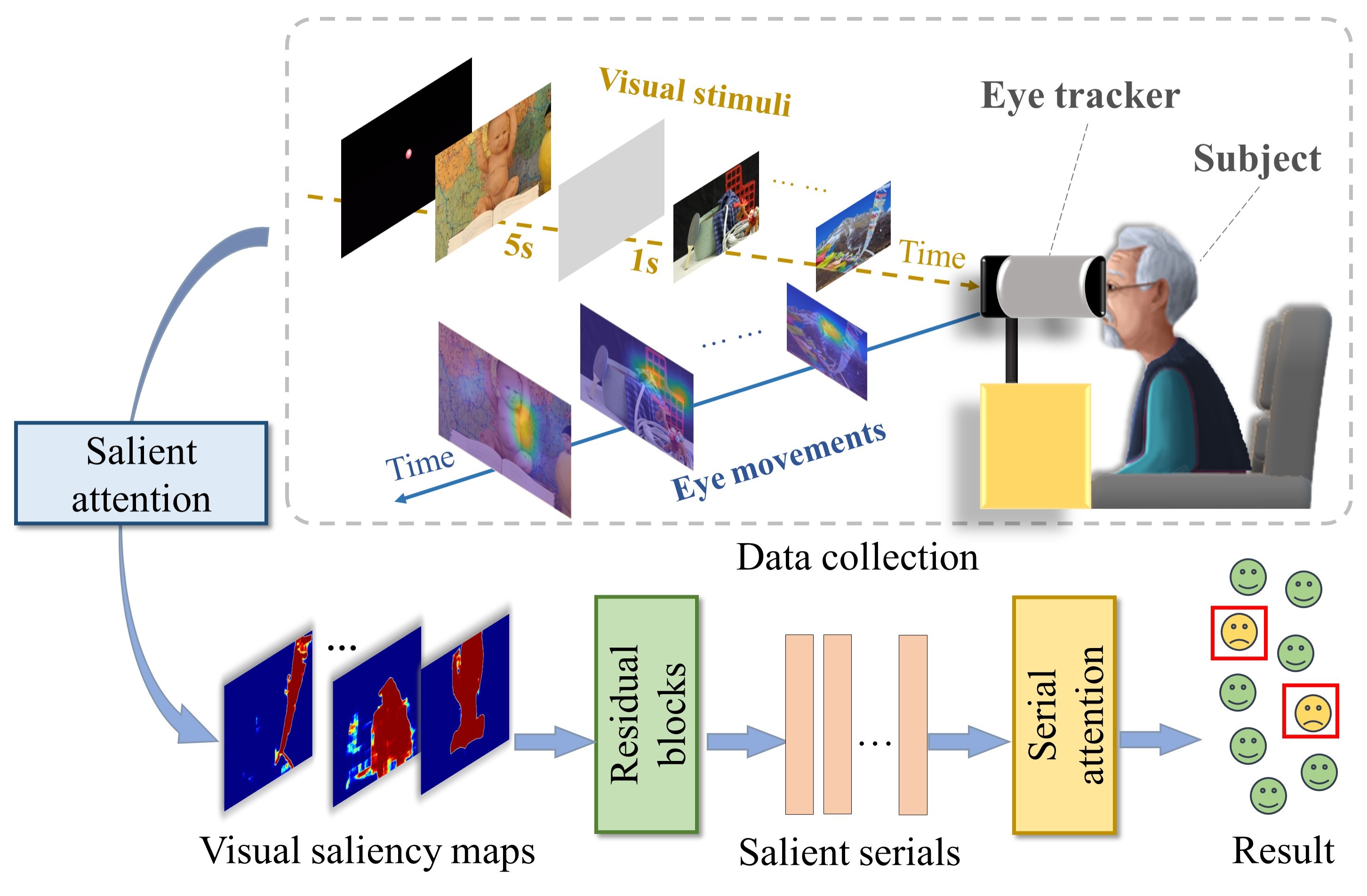
In this paper, we propose a novel approach to diagnose AD using deep learning-based network named Depth-induced Integrated Comparison serial attention Network (DISCN) with eye movements collected during a free viewing task. As shown in Fig. 7, a series of images in left and right eye perspectives are presented to subjects binocularly by an 3D eye tracker designed by Sun et. al [26], which records eye movements of subjects and transforms eye movements into heatmaps. Then, 3D visual stimuli and heatmaps are integrated into visual saliecy maps by an integration module. The visual saliency maps are processed by a serial attention module to get a diagnosis result. The major contributions of this paper are summarized as follows:
-
•
Targeting at the diagnosis of AD with eye movement data, we proposed a novel deep learning-based DISCN, which contains an integration module to fuse visual stimuli with eye movements for evaluating visual saliency maps comprehensively. serial attention module is applied to extract visual saliency features from the visual saliency maps, so that the AD detecting accuracy is enhanced.
-
•
We conducted extensive experiments on a collected eye movements dataset and completed comprehensive comparison, The results showed our approach outperformed the state-of-the-art models.
II Related Work
II-A AD diagnosing methods based on eye movements
Saccade eye movement including saccade latency, saccade errors [38, 39, 40] are commonly used for AD diagnosis. It aims to establish an evaluation criteria for the detection of abnormal eye-tracking behavior in AD patients for the initial diagnosis of AD patients by well-designed clinical eye-tracking tests. Eraslan et. al [38] designed a saccade task that is applied on patients with AD and Mild Cognitive Impairment (MCI), and healthy controls, which found that both AD patients and MCI showed varying degrees of elevated antisaccade error rates and reduced saccade accuracy compared to healthy controls. This suggests that cognitive impairment in AD patients is highly correlated with abnormal saccade performances, which gives a promising eye-movement indicator for the initial diagnosis of AD patients.
To simplify the process of saccade tasks and provide a more natural experience, Hannonen et. al [39] designed a shorter reading task that detected subjects’ saccade behaviors including saccade speed, saccade amplitude, and saccade frequency during reading, which found that AD patients performed worse in the reading test compared with healthy controls. To further confirm the correlation between the results of the eye hopping task and the traditional medical diagnosis of AD, Eraslan et. al [40] performed saccade tests and neuropsychological tests on AD patients and healthy controls respectively. The result showed that the rate and amplitude of saccade correlated strongly with the neurological test results , which allowed for an accurate diagnosis of AD patients.
In order to get more consistent diagnosis of AD, researchers have explored more diverse eye movement indicators to diagnose AD in addition to saccades, and have designed more comprehensive eye movement tests [41, 42]. Tokushige et. al [41] designed a visual memory task to record and analyze the visual search processes and visual attention of AD patients and healthy controls while performing the task. The results showed that AD patients paid insufficient attention to the informational parts and required longer time for right visual exploration. This suggested that visual attention and visual exploration processes are also promising eye movement indicators for the diagnosis of AD. In addition, to obtain more comprehensive eye movement diagnostic indicators, Jang et. al [42] designed a picture depiction task and assessed the subjects from multiple dimensions such as saccade, gaze, visual attention, and verbal ability, which verified that the multimodal eye movement indicators had superior stability for AD diagnosis.
II-B Serial attention neural networks
With the increasing demand for intelligent and efficient AD diagnosis, deep learning methods are increasingly being applied to the analysis of AD diagnostic data containing eye movements. Jang et. al [42] utilized a machine learning-based deep classification neural network to extract features from multimodal eye movement indicators for AD diagnosis. Pereira et. al [52] also introduced machine learning to process eye movements collected in visual search tasks. In order to take full advantage of the deep learning network’s ability to process different categories of data, Barral et. al [53] designed deep learning-based classifiers to extract eye movement features and language features respectively of subjects in a visual search task, and fused the two features for AD diagnosis.
Although these experiments have demonstrated that deep learning can efficiently and intelligently process eye movement data and can be used in AD diagnosis, there is a relative lack of application of attention modules in the network architectures, even though attentional mechanisms have been shown to be effective in processing multimodal information.
As an important conception in deep learning field, attention neural network tends to focus on the distinctive parts when processing large amounts of information, which has been widely used in diverse application domains [43]. The most commonly used domains for attention modules are natural language processing (NLP) [44, 49, 50] and computer vision (CV) [45, 47, 48]. For example, local attention has been verified by Luong et. al [46] to improve translation performance by focusing on a portion of the words in the source sentence at a time. Mnih et. al [45] presented a spatial attention model that is formulated as a single RNN that takes a glimpse window as its input and uses the internal state of the network to select the next location to focus on as well as to generate control signals in a dynamic environment.
To exploit the superiority of visual attention modules in eye movement analysis, we used the visual attention module in the free viewing task to extract visual saliency information between the visual stimulus and eye movements. We also utilized the serial attention module in the saliency comparison process due to the temporal nature of the eye movement data, which allowed the network to give more attention to abnormal eye movement behaviors.
Although a variety of eye movement indicators have been shown to be valid in the early diagnosis of AD, very limited studies have focused on the correlation between eye movements and visual stimuli in eye movement analyses. It has been demonstrated that the saliency distribution of the visual stimulus that elicits the eye movement behaviors affects the differentiation between AD patients and healthy controls [34], so that a joint analysis of visual stimuli with the corresponding eye movements can lead to more objective diagnostic results.
To overcome this drawback, we designed an image free-viewing task and jointly analyzed the saliency distribution of visual stimuli with the corresponding eye movements. We performed a comparative analysis based on the saliency of visual stimuli and eye movements, and made a diagnosis of AD based on the degree of their correlation.
III Method
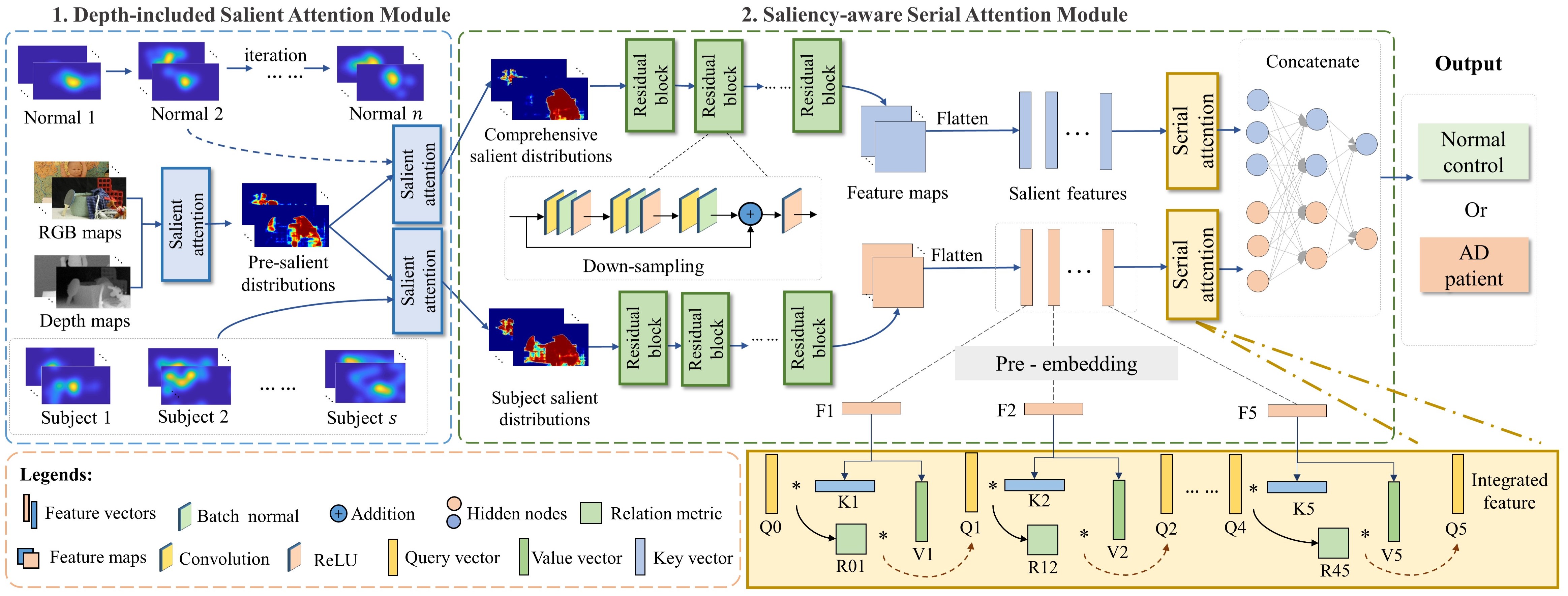
In this section, we introduce our proposed DISCN in detail, including the notations and preliminaries, the mathematical descriptions of the two parts in DISCN: a depth-included salient attention module and a saliency-aware serial attention module as shown in Fig. 2. The main idea is to jointly analyse the salient distributions of visual stimuli and the corresponding visual attention to detect the abnormal eye movements of AD patients caused by cognitive declines. To evaluate comprehensive salient distributions of visual stimuli, the RGB-D images and normal heatmaps are integrated with the salient attention module proposed in [58]. Meanwhile, a saliency-aware serial attention module is introduced to merge temporal features separately from salient distributions of visual stimuli and subjects. Finally, multi-layer perception (MLP) is used as a classifier, and the result of which is considered as a diagnosing result.
III-A Notations and preliminaries
In the following subsections, we represent a set of 3-channel images with notation I along with meaningful superscripts and subscripts, e.g., denotes a set of original images of visual stimuli. T is defined as a set of tokens, which is composed of single tokens t, i.e., . The feature maps calculated by residual layers are defined as F, and feature vectors are defined as v. Other matrices used in the paper are represented by uppercase bold letters, and vectors are represented by lowercase bold letters. The dimensions and meanings of all notations will be explained after it is defined.
III-B Depth-included salient attention module for preliminary saliency map evaluation of visual stimuli
The salient attention module is used for integrating original images and depth images of visual stimuli, as well as integrating visual stimuli and heatmaps that represent human visual attention with attention structures. The original images and depth images of visual stimuli are firstly integrated to evaluate preliminary saliency maps with a salient attention (SAA) block, which is constructed by ”Image-to-Token” (I2T) layers, “Tokens-to-Token” (T2T) layers [61], transformer layers [62], ”Cross-Modality Transformer” (CMT) layers, and ”Token Attention” (TA) layers. The whole process of integrating original images and depth images of visual stimuli by SAA is defined as follows:
| (1) |
where are the original images (RGB images) and depth images of the visual stimuli, which have channels and size of . and are the intermediate tokens in the saliency map evaluation process, where is the number of tokens of each visual stimulus, and is the dimension of each token. is the preliminary saliency maps evaluated from original and depth images, which have the same size. The function represents the transformer structure [62] of sequence-to-sequence mode that can model global dependencies among all pixels in the whole image. The main functions and the variables are explained as follows:
-
•
Image to Tokens
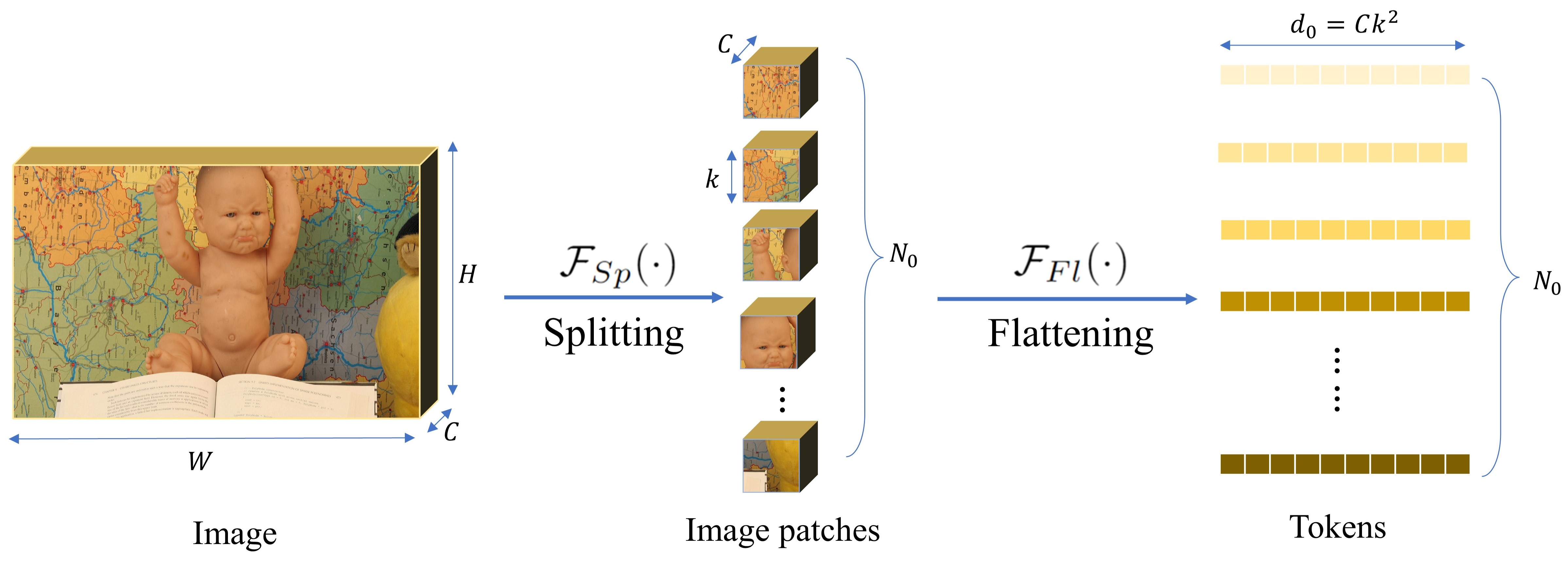
Figure 3: The process of I2T that consists of a splitting step and a flattening step for converting an image into tokens. denotes the operation that converts an image into a set of vectors i.e. tokens, which includes two steps: splitting and flattening, as shown in Fig. 3.
(2) where denotes the operation of splitting images into image patches, and is the operation of flattening image patches by pixel.
-
•
Tokens to Token

Figure 4: The process of T2T that consists of transformers, a reshaping step and a soft-split step for converting input tokens into high-dimensional tokens. denotes the operation that convert tokens into high-dimensional tokens with two transformers, a reshaping step and a soft-split step, as shown in Fig 4. is defined as follows:
(3) where is the reshaping step that combines tokens into metrics, and is the soft splitting function that splits the high-dimensional images into new vector sets in a manner like convolution. The window size of each split is with a padding of pixels and a stride of . Pixels in each window are connected by the channel dimension to get high-dimensional tokens. The dimensions of tokens are converted from into in the th T2T layer, where and . Then a transformer is conducted to the high-dimensional tokens and finally get the output tokens , where is the number of T2T layers.
-
•
Cross-Modality Transformer
A CMT layer is adopted to combine the two set of tokens from original and depth images separately to get cross-modality tokens . Function as follows:
(4) where are the query, key and value vectors of original and depth images, are learnable matrices for linear embedding from tokens into query, key, and value vectors. are tokens that combines information from both original images and depth images. Then the two output tokens are concatenated and projected linearly into a token set . is a learnable matrix for linear projection, and denotes concatenation by the token number dimension .
-
•
Reversal Tokens to Token
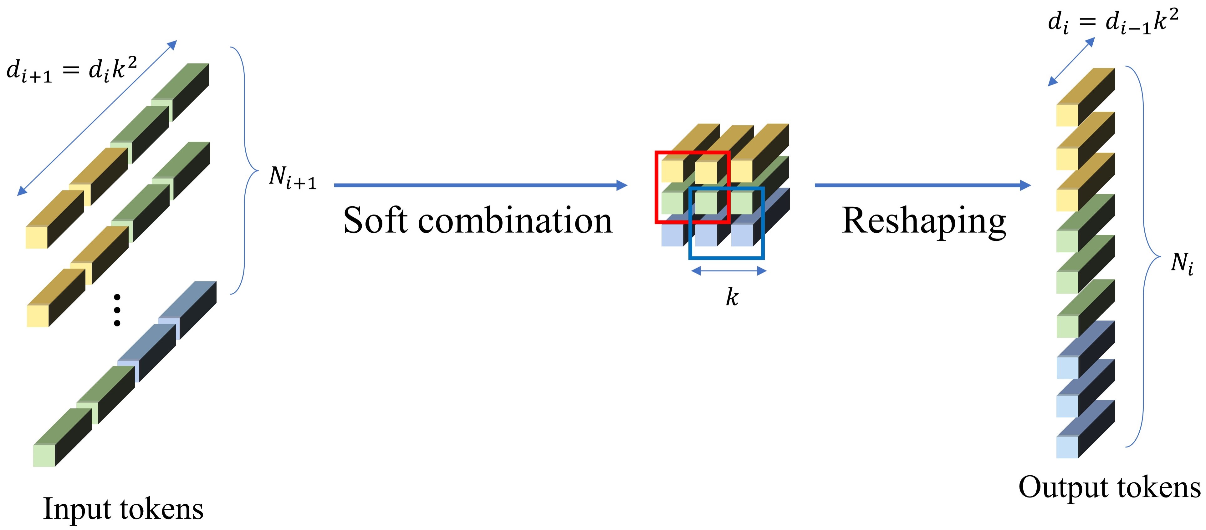
Figure 5: The process of reversal T2T that consists of a soft-combine step and a reshaping step for converting high-dimensional tokens into more lower-dimensional tokens. The reversal tokens to token operation is a reversal process of T2T, and is represented with . Reversal T2T aims to recover the high-dimensional tokens into their original shapes. As shown in Fig. 7, is defined as follows:
(5) where is the reversal process of soft splitting, and is the reversal process of reshaping. Reversal T2T is applied on twice in a residual manner:
(6) where are the outputs of each reversal T2T operation. Among them, , where the first token is seen as the salient token to learn the salient information from the whole token set .
-
•
Token Attention
A Token attention (TA) mechanism is adopted for saliency evaluation, which is defined as follows:
(7) where are the tokens of token set , are the query,key and value vector of salient token . are learnable matrices for linear projection. are the query vectors of the rest tokens, and are learnable matrices for linear projection. The output tokens and compose the salient token set . The salient token set is reshaped into a preliminary saliency map by a reversal T2T function.
III-C Salient attention module for integrating visual stimuli with human visual attention
The human visual attention can be represented by heatmaps of the same shape with visual stimuli. Heatmaps are divided into two sets: a normal set and a subject set . The contains heatmaps of normal controls. contains heatmaps of subjects including 1:1 normal controls and AD patients that need to be classified. The definitions of and are as follows:
| (8) |
where are the heatmaps corresponding to visual stimuli. For the subject set, preliminary saliency maps are integrated with heatmaps of each individuals with SAA module mentioned in Section III-B:
| (9) |
where repersents the saliency maps of the th subject containing salient information of both visual stimuli and human visual attention. As for the normal control set, heatmaps are integrated with preliminary saliency maps in an iterative manner:
| (10) |
where denotes the comprehensive saliency maps that includes visual salient information of both RGB-D visual stimuli and normal controls. are the intermediate images of the th iteration.
III-D Saliency-aware serial attention module for feature fusion
The saliency-aware serial attention module will extract visual saliency-aware features from the two sets of saliency maps, and fuse the features with serial attention module.
Given the th subject saliency maps and the comprehensive saliency maps , residual blocks are implemented on the two sets of saliency maps separately in cascade. The th residual block is defined as function :
| (11) |
where are the outputs of the th residual block, where and . denotes a convolutional layer, denotes a batch normalization layer and denotes a ReLU activation layer. are the feature maps of th residual block. indicates up-sampling operation on the dimension. residual blocks are applied on and , and get feature maps of the th residual layer, which are flattened into vector sets , where . and are the serial features in temporal order of comprehensive and subject saliency maps respectively, where . The serial features are preliminarily embedded into feature serials and , where :
| (12) |
where is matrices used for preliminary embedding. Then the feature serials are embedded into key and value vectors:
| (13) |
where are matrices for prelimibary embedding. are keys and values of the th vector in the feature serial. The vectors in feature serial are integrated by serial attention module:
| (14) |
where and are learnable parameters. and are calculated by previous features and , which presents the temporal order of the serial. and are concatenated into vector :
| (15) |
where is the final vector in serial attention, which is inputted into a 2-layered MLP:
| (16) |
where , are linear matrices, and is the classification result, whose first item represents the probability that the th subject is diagnosed as an AD patient. A binary cross entropy loss (BCE) is applied to calculate the classification loss by and the label of th subject :
| (17) |
In the convergence procedure, all the learnable parameters of DISCN are updated by backward gradient descent, which propagates the gradient information of each parameter through the entire DISCN and optimizes all the parameters according to the fitting loss. Parameters could be updated in each training ergodic of all items in the training dataset:
| (18) |
where denotes all parameters and decides the rate of parameters updating, namely learning rate. With enough epoches, all parameters will be updated until the loss function reaches its stable and minimum value, which indices that the proposed model is at its optimum state of best-fit the predictions to labels.
IV Experiments
In this section, we introduce the basic information of participants in our projection and the eye movements collection process. We also visualize the process of comprehensive visual saliency evaluation. The designs and results of comparison experiments and ablation experiments with implementation details are presented in this section.
IV-A Participants
A total of 150 participants including 50 early AD patients and 100 normal controls are recruited in our study. The AD patients (23 males and 27 females) were aged from 54 to 84 years old who were recruited form the cognitive impairment clinics of Huanhu Hospital in Tianjin, China (http://www.tnsi.org/). All AD patients met NINCDS-ADRDA criteria [60]. In AD patients, humans with uncorrected dysfunctions of vision or hearing loss, mental disorders, or other symptoms that made them unable to complete the proposed free viewing task. The normal controls were recruited from age matched friends and relatives of patients who had no subjective or informant-based complaints of cognitive decline. The use of eye-tracking data for analysis of AD patients’ cognitive decline obeyed the World Medical Association Declaration of Helsinki [36].
As shown in Section III-C, we divide the 150 participants into a “subject set” and a “normal set” . is composed with 50 normal controls, and the remaining 50 AD patients and 50 normal controls form , namely , . Heatmaps in are used for iterative fusion with the visual stimuli, and participants in need to be diagnosed. is divided equally into five subsets to implement 5-fold cross-validation, as shown in TABLE I.
| Training set | Testing set | Sum | Label | |
| AD patients | 40 | 10 | 50 | 0 |
| Normal controls | 40 | 10 | 50 | 1 |
| Sum | 80 | 20 | 100 | 0/1 |
IV-B Eye movements collection
To collect eye movements of the participants under stereo visual stimuli, we perform a free viewing trial with a noninvasive binocular eye tracker. The eye movements collected from the free viewing trial are presented in the form of heatmaps.
IV-B1 Stereo visual stimuli designs
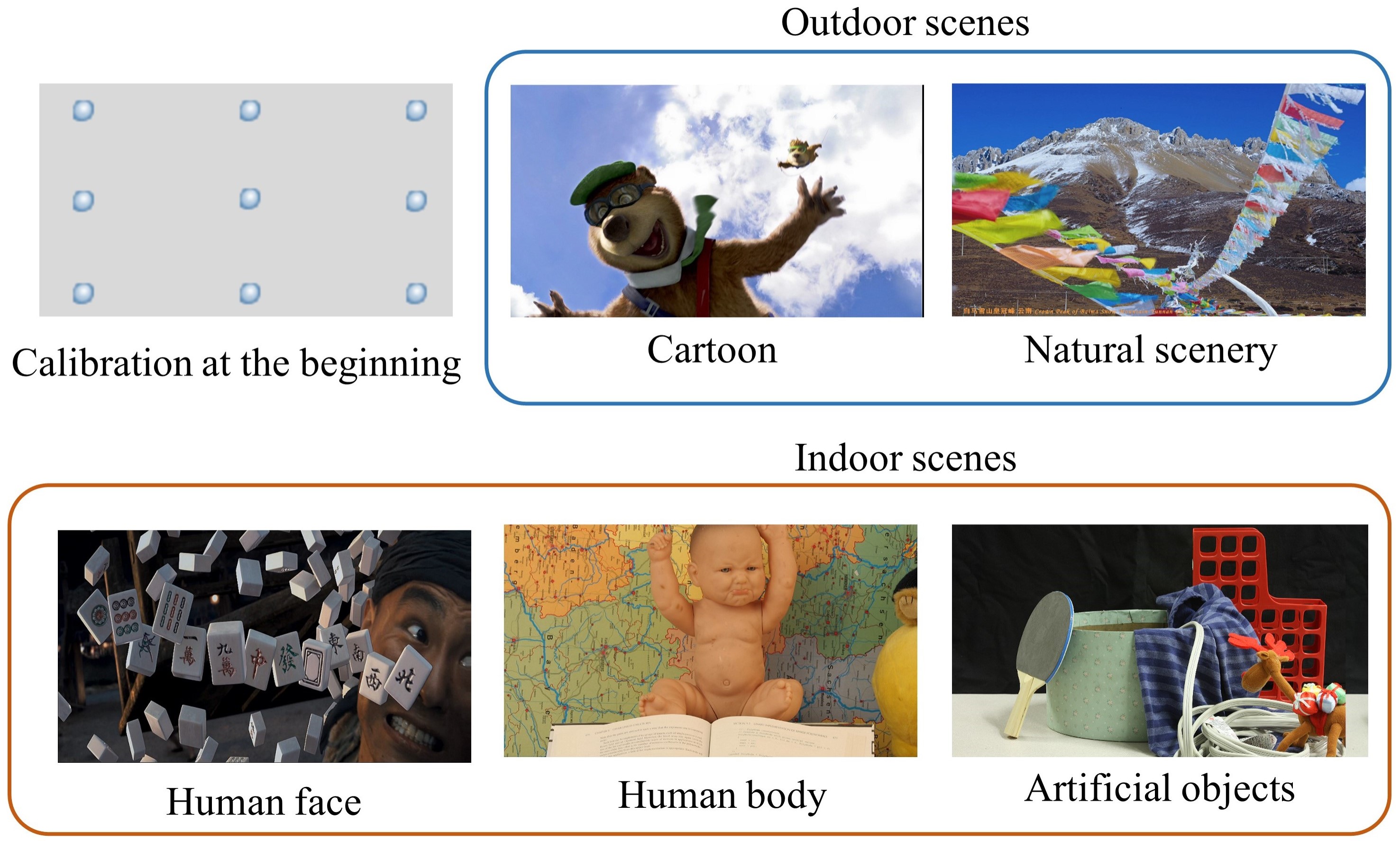
The stereo visual stimuli is a video including a calibration procedure at the beginning and a serial of images. The calibration procedure was applied to the participants for a more accurate eye movement estimation. After that, five images were displayed for 5 seconds through binocular stereo vision with a 1-second gap between each two of them. The contents of the stimuli contained indoor scenes, outdoor scenes with different styles including natural scenery, artificial objects, cartoon, human face and human body, which is presented in Fig. 6. The depth maps corresponding to each RGB visual stimulus were achieved by calculating the disparities between the images of left-eye and right-eye views.
The whole display of visual stimuli only took less than 1 minute for each participant, which satisfies the requirements of efficiency for large-scale AD diagnosis screening. The design of binocular vision mode is for introducing depth to stimulate richer brain and eye movement activities [54]. Diverse visual stimuli can provide subjects with different viewing experiences and stimulate rich eye movements to the maximize extent.
IV-B2 Noninvasive eye tracker
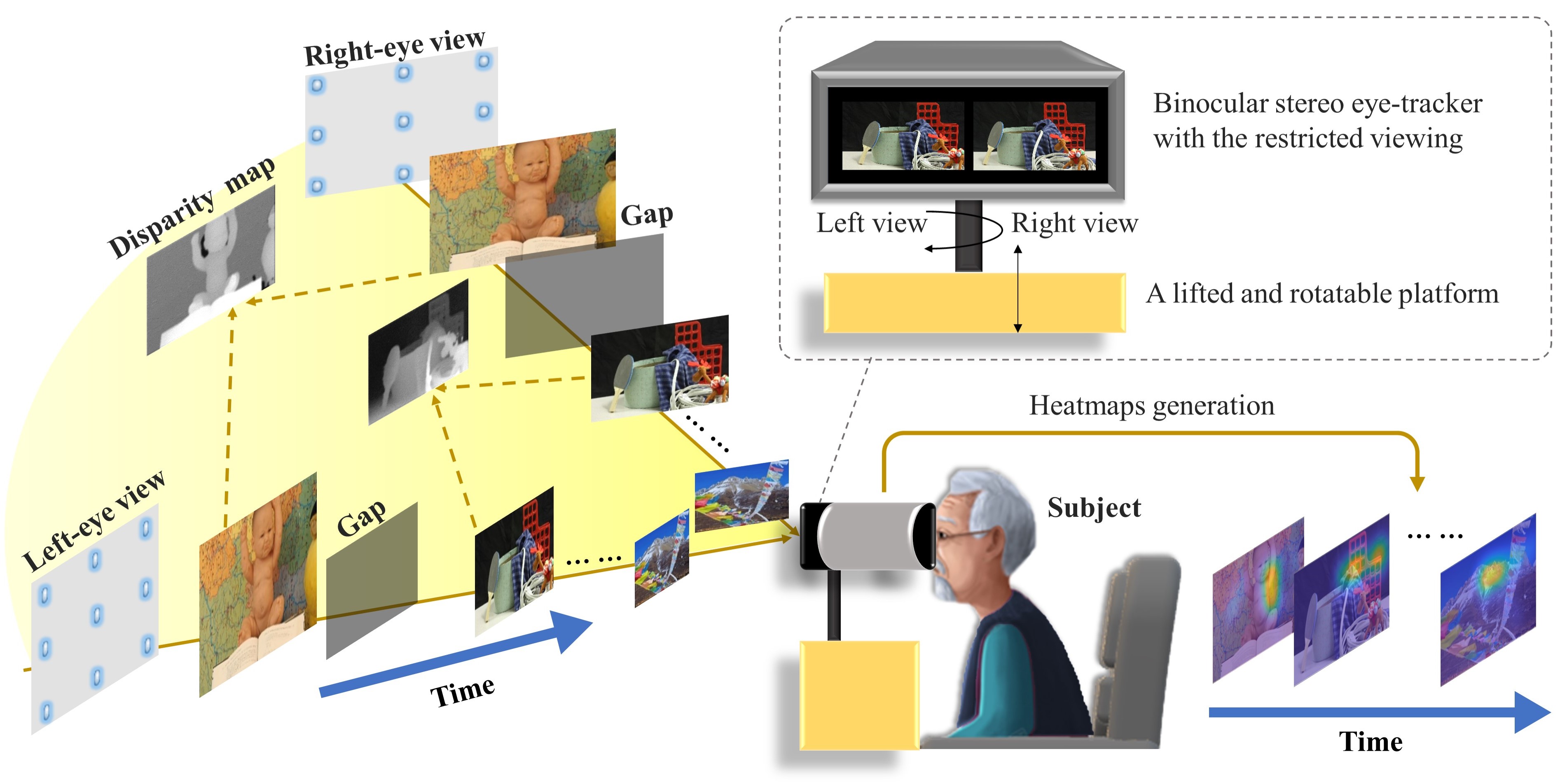
During the free viewing task, eye movements of participants are recorded using an eye tracker with the stereo stimuli designed by Sun et al. [26], this eye tracker estimates gaze positions at an average error of 1.85cm/0.15m over the workspace volume 2.4m4.0m7.9m. It displays stereo visual stimuli in the resolution of 19201080@120 Hz in a limited vision without requiring the viewer to wear any accessories, which is friendly to participants, especially to the elders. The eye tracker can be adjusted in a 360-degree direction freely to meet the need of different users. It allows participants to experience a 3D immersive viewing by displaying the images of left-eye and right-eye perspectives separately through two sets of lenses. The eye movements are also collected in binocular vision by the inside cameras.
IV-B3 Heatmaps of visual attention
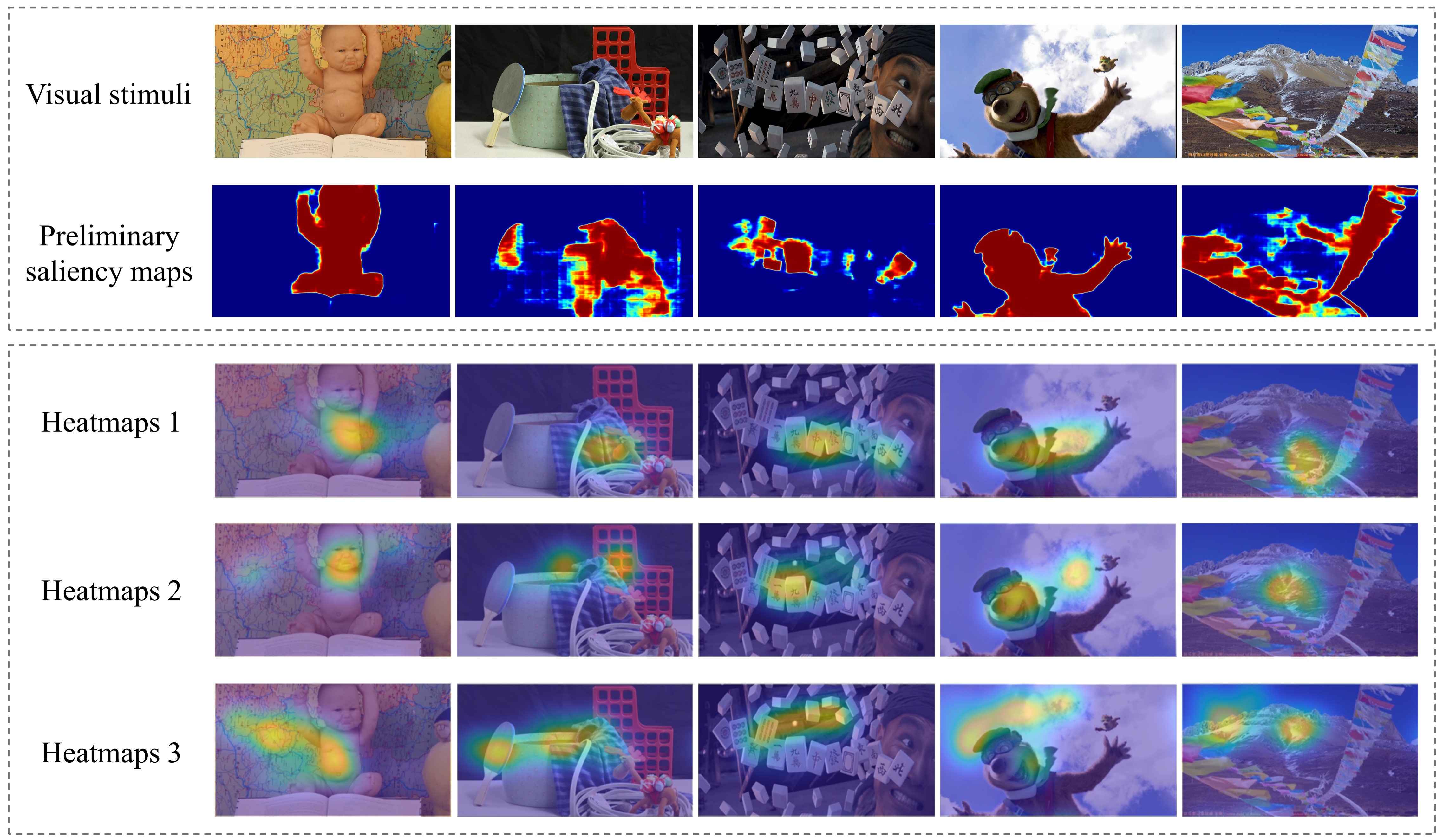
The collected eye movements are transformed into heatmaps by iMap [55], which reflect the distributions of visual attention. The generated heatmaps are the inputs of the proposed DISCN together with the RGB maps and depth maps of corresponding visual stimuli.The heatmaps are evaluated with gaze positions and duration of each individual. In the heatmaps, color represents the duration-weighted spatial density of human gaze points, which reflects the visual attention level. The warmer color a region shows, the more visual attention an individual pays to it, as shown in Fig. 8.
IV-C Experiment designs
IV-C1 Ablation experiments
The effectiveness of four modules in DISCN are verified, including depth integration, normals integration, residual feature extraction, and feature fusion. For depth integration and normals integration, we first visualize the process of evaluating comprehensive salient distributions for qualitative analysis. Then two models named noDEP and noNOR are designed to compare with DICSN. As for residual feature extraction and feature fusion, we further design corresponding models named noRES and noSEA for ablation. The models are introduced as follows:
-
•
noDEP: Depth affects the visual perception of subjects. In noDEP, original maps is integrated with normals directly by only one SAA.
-
•
noNOR: Healthy visual attention is combined with pre-salient maps in DISCN. noNOR take only pre-salient distributions to compare with subject salient distributions.
-
•
noRES: Residual blocks contain hierarchical residual structures that can address a common degeneration problem. In noRES, residual blocks are replaced with traditional CNN layers with the same depth.
-
•
noSEA: Serial attention module (SEA) fuses serial vectors in order, that models the temporal variations of salient features according to the order of visual stimuli. In noSEA, SEA is replaced by MLP layers.
Moreover, four feature fusing modules including MLP, GRU, LSTM and SEA are applied in DISCN to verify the effects. Among them, MLP fuses salient features with pure fully-connections and activation layers without temporal orders; GRU and LSTM are recurrent structures controled by gates, which receive features in order; SEA fuses salient features with both temporal orders and attention mechanism.
IV-C2 Feature extraction structures
To further explore the effects of different feature extraction and fusion module, three different feature extracting mechanisms including pure convolution (CNN), multi-scaled feature complementary (MSBPNet), and residual blocks (DISCN) are also tested based on the four feature fusing methods. The results validate the effectiveness of the network structure adopted by the DISCN from two dimensions: feature extraction and fusion.
IV-C3 Comparison experiments
In this part, the performance of DISCN against the following methods are tested: CNN[27], GoogLeNet[21], self-regulated network (RegNet)[22], Multi-Scale Binary Pattern Encoding Network (MSBPNet)[24] and MixPro[65]. It is worth noting that the performances based on MLP and SEA are compared to further verify the significance of SEA module.
-
•
CNN[27]. CNN is a traditional image processing architecture and serves as a fundamental component of multiple image classification networks. It is designed to solve image pattern recognition tasks with a simpler structure than artificial neural networks (ANNs).
-
•
GoogLeNet[21]. GoogLeNet is a deep convolutional neural network that utilizes an efficient deep neural network architecture for computer vision, called Inception, to ensure agreement with limited computational resources.
-
•
RegNet[22]. RegNet is a variant of ResNet that introduces a memory mechanism into traditional ResNet to extract potentially complementary features. This approach has shown to be effective at extracting spatiotemporal information from images.
-
•
MSBPNet[24]. MSBPNet can effectively identify and leverage the patterns of multiple scales in a cooperative and discriminative fashion within a deep neural network, providing superior capability for pathology image analysis, such as cancer classification.
-
•
MixPro[65]. MixPro combines MaskMix and Progressive Attention Labeling with transformer-based network as data augmentation methods, to achieve better performance and robustness.
IV-C4 Implementation details
The implementation details of all experiments are as follows: all the networks are trained using SGD optimizer (momentum=0.9). The batch-size is set to 16. Learning rate is set to . All layers are initialized using the initialization scheme proposed by He et. al [57]. A cross entropy is adopted as a loss function and we also used regularization.The central region of 224224 pixels is cropped for all heatmaps. All experiments are implemented on PyTorch platform and executed on a workstation with two 4080Ti GPUs. All the networks are trained using an early stopping strategy with “UP criterion” [56] to prevent the overfitting problem.
IV-D Experiment results
IV-D1 Visualization of depth/normals integration
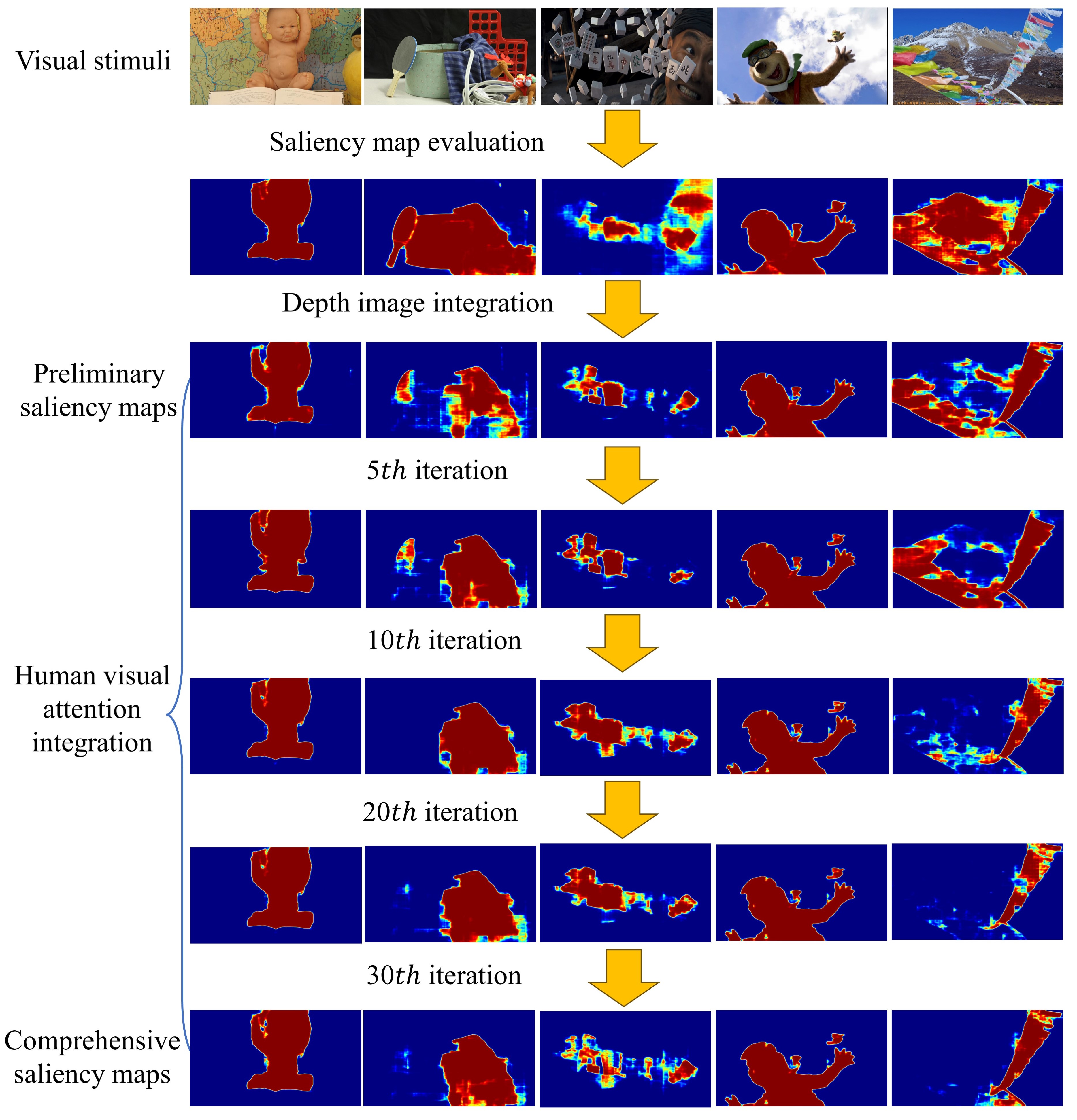
The process of comprehensive saliency maps evaluation has been introduced in Section III-C. By integrating with depth maps the evaluation of saliency maps are corrected with more details. By introducing depth maps, the saliency of objects in the background areas decreases, e.g. the human fave and mountain in the background. Moreover, by introducing visual attentions of normal controls, normal human visual attention further corrects the saliency maps and adds more details matching common visual habits of normal controls. For example, although the cartoon bear behind is judged as less salient object with the introduce of the depth map, it is seen more salient as introducing visual attention of more normal controls. The whole process is presented in Fig. 9.
IV-D2 Ablation experiments
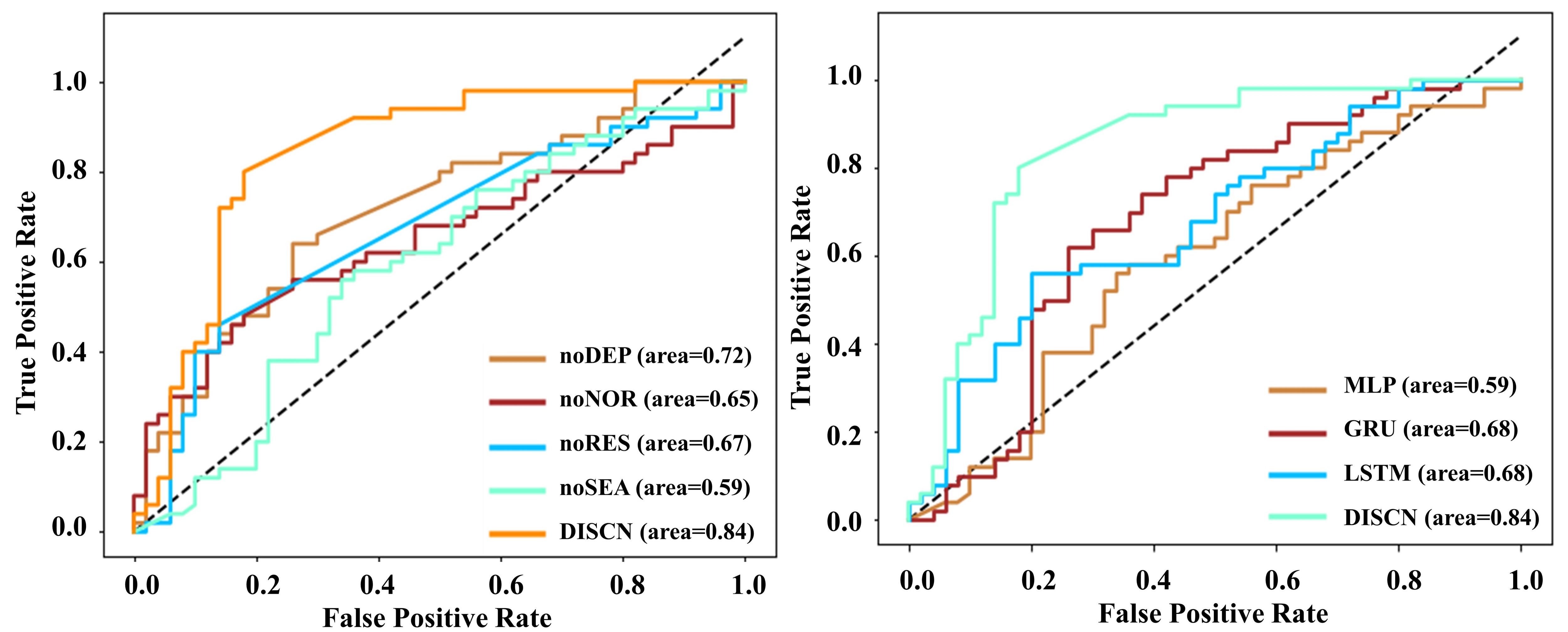
The results of ablation experiments are shown in Fig. 10 and TABLE II and III separately. From TABLE II we can see that, depth integration and normals integration contributes 0.13 and 0.17 accuracy to DISCN. The residual feature extractor contributes 0.17 accuracy, as features extracted by deep convolutional layers can not represent visual saliency adequately without features of shallow layers. SEA is the most important module as it contributes 0.23 accuracy to DISCN, which indicates that SEA is efficient for salient feature fusion.
Additionally, TABLE III validates performances of DISCN with four feature fusing modules. From TABLE III it can be concluded that recurrent structures with temporal order perform better than MLP. SEA, as a fusing structure that contains both temporal order and attention, performs the best. The ROC curves of two sets of models are plotted in Fig. 10, which is consistent with tables and shows the superior of DISCN from statistical perspective.
| Metrics | noDEP | noNOR | noRES | noSEA | DISCN |
| Accuracy | 0.680.01 | 0.640.02 | 0.640.01 | 0.580.01 | 0.810.01 |
| Recall | 0.660.04 | 0.480.08 | 0.420.05 | 0.380.11 | 0.800.01 |
| Precision | 0.760.02 | 0.600.11 | 0.850.02 | 0.650.14 | 0.860.02 |
| F1-score | 0.660.01 | 0.520.08 | 0.500.04 | 0.400.05 | 0.810.01 |
| AUC | 0.680.01 | 0.640.02 | 0.640.01 | 0.580.01 | 0.810.01 |
| Metrics | MLP | LSTM | GRU | SEA |
| Accuracy | 0.580.01 | 0.650.01 | 0.660.02 | 0.810.01 |
| Recall | 0.380.11 | 0.560.03 | 0.840.03 | 0.800.01 |
| Precision | 0.650.14 | 0.690.02 | 0.640.02 | 0.860.02 |
| F1-score | 0.400.05 | 0.600.02 | 0.710.01 | 0.810.01 |
| AUC | 0.580.01 | 0.650.01 | 0.660.02 | 0.810.01 |
IV-D3 Feature extracting structures
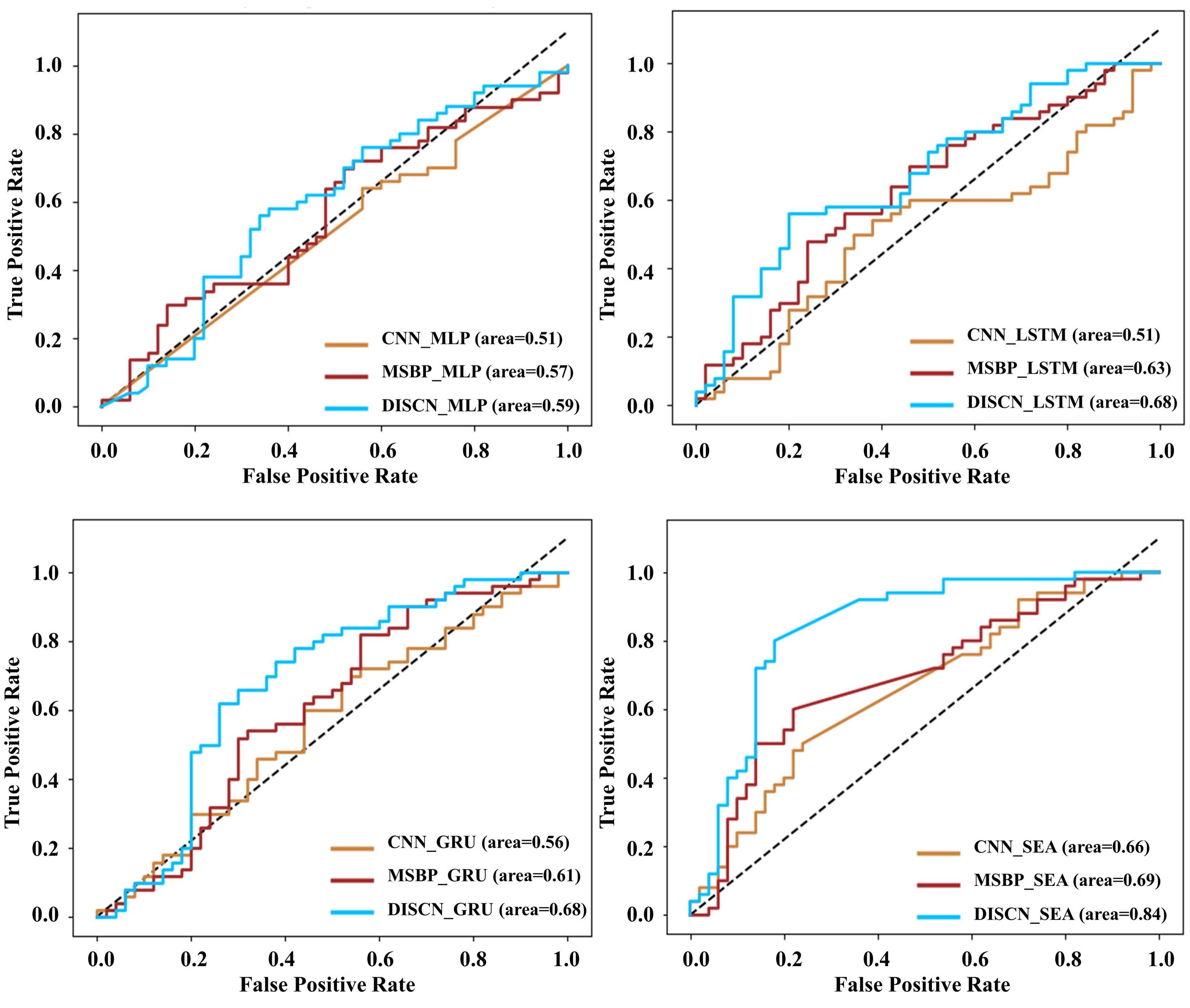
The effectiveness of three feature extracting structures with four different feature fusing modules are verified in TABLE IV and Fig. 11. In TABLE IV, three feature extracting structures perform worst with MLP, and the difference of performances are not significant. The performances of LSTM and GRU is intermediate, and the differences of performances appear more significantly. MABPNet with multi-scaled features performs better than CNN with pure convolution, and DISCN with multi-layered residual layers performs the best. As for structures with SEA, differences between models are most significant, DISCN performs the best, MSPBNet performs intermediately and CNN performs the worst. For the same feature extracting structure, it performs the best based on SEA, intermediately based on GRU and LSTM, and the worst based on MLP. Fig. 11 shows consistent results with TABLE IV from statistical perspective.
| Feature extractor | Metrics | MLP | LSTM | GRU | SEA |
| CNN | Accuracy | 0.530.01 | 0.540.01 | 0.570.01 | 0.630.01 |
| Recall | 0.620.19 | 0.320.14 | 0.680.13 | 0.500.06 | |
| Precision | 0.510.10 | 0.430.15 | 0.610.01 | 0.730.02 | |
| F1-score | 0.470.07 | 0.300.07 | 0.570.01 | 0.530.04 | |
| AUC | 0.530.01 | 0.540.01 | 0.560.03 | 0.630.01 | |
| MSBPNet | Accuracy | 0.590.01 | 0.600.01 | 0.660.01 | 0.680.01 |
| Recall | 0.720.09 | 0.440.08 | 0.700.04 | 0.600.02 | |
| Precision | 0.610.01 | 0.780.04 | 0.700.01 | 0.770.02 | |
| F1-score | 0.600.02 | 0.490.01 | 0.670.01 | 0.640.01 | |
| AUC | 0.590.01 | 0.600.01 | 0.660.01 | 0.680.01 | |
| DISCN | Accuracy | 0.580.01 | 0.790.06 | 0.660.02 | 0.810.01 |
| Recall | 0.380.11 | 0.710.01 | 0.840.03 | 0.800.01 | |
| Precision | 0.650.14 | 0.860.02 | 0.640.02 | 0.860.02 | |
| F1-score | 0.400.05 | 0.770.01 | 0.710.01 | 0.810.01 | |
| AUC | 0.580.01 | 0.790.07 | 0.660.02 | 0.810.01 |
IV-D4 Comparison experiments
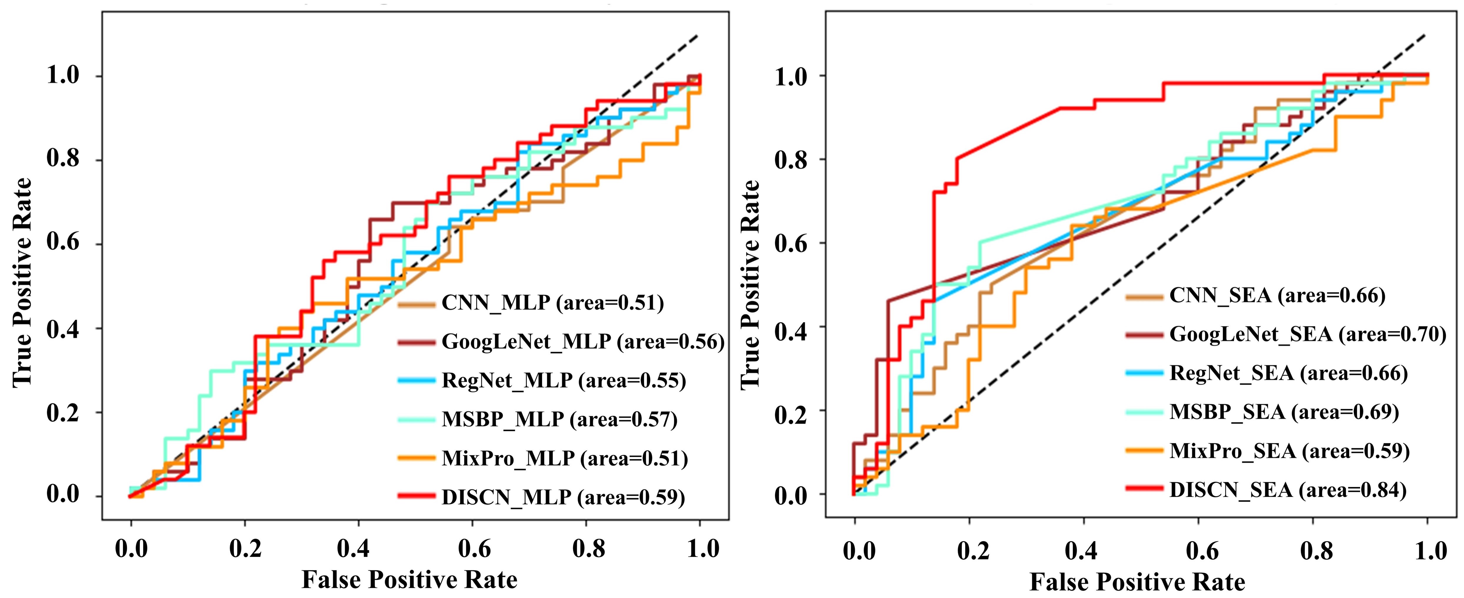
TABLE V and Fig. 12 depict the detailed performances of all state-of-the-art methods and the proposed DISCN. The following observations can be made from TABLE V and Fig. 12: 1) Our proposed DISCN outperforms all state-of-the-art methods equipped with two different feature fusing modules by a significant margin. 2) CNN and GoogLeNet, as convolutional feature extracting structures, use relatively shallower features for classification. The two models perform better based on SEA than MLP, which proves that it is feasible to use simple convolutional features of image for classification, and the temporal attention mechanism in SEA can better improve network performance; 3) RegNet and MixPro are heavyweight networks and use complex image features. They perform the worst, indicating that overly complex networks may not be suitable for simple eye movement feature extraction due to issues like overfitting. 4) MSBPNet is also heavyweighted but outperforms RegNet and MixPro, which is benifited by the residual like multi-scaled feature integration mechanism; 5) Models that use SEA module consistently perform better than MLP, as SEA introduces temporal orders of salient features, and focuses on information from feature vectors that is critical for AD diagnosis, enabling the model to make more accurate judgments.
| Metrics | MLP | SEA | Improvement | |
| CNN[63] | Accuracy | 0.530.01 | 0.630.01 | 0.10 |
| Recall | 0.620.19 | 0.500.06 | 0.12 | |
| Precision | 0.510.10 | 0.730.02 | 0.22 | |
| AUC | 0.530.01 | 0.630.01 | 0.10 | |
| F1-score | 0.470.07 | 0.530.04 | 0.06 | |
| GoogLeNet[21] | Accuracy | 0.600.01 | 0.690.01 | 0.09 |
| Recall | 0.660.08 | 0.460.06 | 0.20 | |
| Precision | 0.690.04 | 0.900.02 | 0.21 | |
| AUC | 0.600.01 | 0.690.01 | 0.09 | |
| F1-score | 0.610.01 | 0.560.03 | 0.05 | |
| RegNet[22] | Accuracy | 0.560.01 | 0.660.01 | 0.10 |
| Recall | 0.820.07 | 0.460.05 | 0.36 | |
| Precision | 0.550.01 | 0.810.01 | 0.26 | |
| AUC | 0.560.01 | 0.660.01 | 0.10 | |
| F1-score | 0.630.02 | 0.550.02 | 0.10 | |
| MSBPNet[24] | Accuracy | 0.590.01 | 0.680.01 | 0.09 |
| Recall | 0.720.09 | 0.600.02 | 0.12 | |
| Precision | 0.610.01 | 0.770.02 | 0.16 | |
| AUC | 0.590.01 | 0.680.01 | 0.07 | |
| F1-score | 0.600.02 | 0.640.01 | 0.04 | |
| MixPro[65] | Accuracy | 0.530.01 | 0.610.01 | 0.08 |
| Recall | 0.300.14 | 0.680.07 | 0.38 | |
| Precision | 0.430.15 | 0.690.04 | 0.27 | |
| AUC | 0.530.01 | 0.610.01 | 0.08 | |
| F1-score | 0.270.07 | 0.610.02 | 0.34 | |
| DISCN | Accuracy | 0.580.01 | 0.810.01 | 0.23 |
| Recall | 0.380.11 | 0.800.01 | 0.42 | |
| Precision | 0.650.14 | 0.860.02 | 0.21 | |
| AUC | 0.580.01 | 0.810.01 | 0.23 | |
| F1-score | 0.400.05 | 0.810.01 | 0.41 |
V Conclusion
In this paper, we propose a novel approach for deep learning-based Alzheimer’s disease (AD) diagnosis called DISCN, which jointly utilizes eye movement and visual stimuli. By leveraging the advantages of multi-image integration module and serial attention module, we effectively integrate visual stimuli and heatmaps that contain eye movements for a more comprehensive visual saliency evaluation. We extract features related to the cognitive impairment of AD patients and send them to the serial attention module for diagnosis. Our experimental results demonstrate that coherent visual saliency of visual stimuli and eye movements is proposing to be used for AD diagnosis. Our network consistently outperforms state-of-the-art methods based on the visual saliency dataset.
Acknowledgement
The authors would like to thank all of the study subjects and their families that participated in the data collection. Sincerely thanks to the reviewers for their efforts in reviewing and improving my paper.
References
- [1] T. T. L. Vuong, B. Song, K. Kim, Y. M. Cho, and J. T. Kwak, “Multi-scale binary pattern encoding network for cancer classification in pathology images,” IEEE Journal of Biomedical and Health Informatics, vol. 26, no. 3, pp. 1152–1163, 2022.
- [2] S. Woo, S. Debnath, R. Hu, X. Chen, Z. Liu, I. S. Kweon, and S. Xie, “Convnext v2: Co-designing and scaling convnets with masked autoencoders,” in Proceedings of the IEEE Conference on Computer Vision and Pattern Recognition, 2023, pp. 16 133–16 142.
- [3] B. Dubois, A. Padovani, P. Scheltens, A. Rossi, and G. Dell’Agnello, “Timely diagnosis for alzheimer’s disease: a literature review on benefits and challenges,” Journal of Alzheimer’s Disease, vol. 49, no. 3, pp. 617–631, 2016.
- [4] Q. Zhou, M. Goryawala, M. Cabrerizo, W. Barker, D. Loewenstein, R. Duara, and M. Adjouadi, “Multivariate analysis of structural mri and pet (fdg and 18f-av-45) for alzheimer’s disease and its prodromal stages,” in Proceedings of the IEEE Conference on the Engineering in Medicine and Biology Society, 2014, pp. 1051–1054.
- [5] D. Chen, A. Alsadoon, P. Prasad, and A. Elchouemi, “Early diagnosis of alzheimer using mini mental state examination method: Mmse,” in Proceedings of the IEEE Conference on Information and Communication Systems, 2017, pp. 125–129.
- [6] C. S. Eke, E. Jammeh, X. Li, C. Carroll, S. Pearson, and E. Ifeachor, “Early detection of alzheimer’s disease with blood plasma proteins using support vector machines,” IEEE Journal of Biomedical and Health Informatics, vol. 25, no. 1, pp. 218–226, 2020.
- [7] G. Palacios-Navarro, J. Buele, S. G. Jarque, and A. B. García, “Cognitive decline detection for alzheimer’s disease patients through an activity of daily living (adl),” IEEE Transactions on Neural Systems and Rehabilitation Engineering, vol. 30, pp. 2225–2232, 2022.
- [8] M. R. Readman, M. Polden, M. C. Gibbs, L. Wareing, and T. J. Crawford, “The potential of naturalistic eye movement tasks in the diagnosis of alzheimer’s disease: a review,” Brain Sciences, vol. 11, no. 11, p. 1503, 2021.
- [9] N. Noiret, B. Vigneron, M. Diogo, P. Vandel, and É. Laurent, “Saccadic eye movements: what do they tell us about aging cognition?” Aging, Neuropsychology, and Cgnition, vol. 24, no. 5, pp. 575–599, 2017.
- [10] A. Coors, M.-A. Imtiaz, M. M. Boenniger, N. A. Aziz, U. Ettinger, and M. M. Breteler, “Associations of genetic liability for alzheimer’s disease with cognition and eye movements in a large, population-based cohort study,” Translational Psychiatry, vol. 12, no. 1, p. 337, 2022.
- [11] J. Liu, Y. Pan, F.-X. Wu, and J. Wang, “Enhancing the feature representation of multi-modal mri data by combining multi-view information for mci classification,” Neurocomputing, vol. 400, pp. 322–332, 2020.
- [12] J. Opwonya, D. N. T. Doan, S. G. Kim, J. I. Kim, B. Ku, S. Kim, S. Park, and J. U. Kim, “Saccadic eye movement in mild cognitive impairment and alzheimer’s disease: a systematic review and meta-analysis,” Neuropsychology Review, vol. 32, no. 2, pp. 193–227, 2022.
- [13] M. A. Parra, J. Granada, and G. Fernández, “Memory-driven eye movements prospectively predict dementia in people at risk of alzheimer’s disease,” Alzheimer’s & Dementia: Diagnosis, Assessment & Disease Monitoring, vol. 14, no. 1, p. e12386, 2022.
- [14] E. Costanzo, I. Lengyel, M. Parravano, I. Biagini, M. Veldsman, A. Badhwar, M. Betts, A. Cherubini, D. J. Llewellyn, I. Lourida et al., “Ocular biomarkers for alzheimer disease dementia: An umbrella review of systematic reviews and meta-analyses,” JAMA Ophthalmology, 2022.
- [15] H. Ramzaoui, S. Faure, R. David, and S. Spotorno, “Top-down and bottom-up sources of eye-movement guidance during realistic scene search in alzheimer’s disease.” Neuropsychology, 2022.
- [16] A. K. Malik, M. Ganaie, M. Tanveer, P. Suganthan, A. D. N. I. Initiative et al., “Alzheimer’s disease diagnosis via intuitionistic fuzzy random vector functional link network,” IEEE Transactions on Computational Social Systems, 2022.
- [17] R. Shi, L. Wang, J. Jiang, A. D. N. Initiative et al., “An unsupervised region of interest extraction model for tau pet images and its application in the diagnosis of alzheimer’s disease,” in Proceedings of the IEEE Conference on Engineering in Medicine & Biology Society, 2022, pp. 2157–2160.
- [18] B. S. S. Varma, G. Kalyani, K. Asish, and M. I. Bai, “Early detection of alzheimer’s disease using svm, random forest & fnn algorithms,” in Proceedings of the IEEE Conference on Innovation in Technology, 2023, pp. 1–6.
- [19] J. Sun, Y. Liu, H. Wu, P. Jing, and Y. Ji, “A novel deep learning approach for diagnosing alzheimer’s disease based on eye-tracking data,” Frontiers in Human Neuroscience, 2022.
- [20] Y. Yin, H. Wang, S. Liu, J. Sun, P. Jing, and Y. Liu, “Internet of things for diagnosis of alzheimer’s disease: A multimodal machine learning approach based on eye movement features,” IEEE Internet of Things Journal, 2023.
- [21] C. Szegedy, W. Liu, Y. Jia, P. Sermanet, S. Reed, D. Anguelov, D. Erhan, V. Vanhoucke, and A. Rabinovich, “Going deeper with convolutions,” in Proceedings of the IEEE conference on Computer Vision and Pattern Recognition, 2015, pp. 1–9.
- [22] J. Xu, Y. Pan, X. Pan, S. Hoi, Z. Yi, and Z. Xu, “Regnet: self-regulated network for image classification,” IEEE Transactions on Neural Networks and Learning Systems, 2022.
- [23] S. Mehta and M. Rastegari, “Mobilevit: light-weight, general-purpose, and mobile-friendly vision transformer,” arXiv preprint arXiv:2110.02178, 2021.
- [24] T. T. Vuong, B. Song, K. Kim, Y. M. Cho, and J. T. Kwak, “Multi-scale binary pattern encoding network for cancer classification in pathology images,” IEEE Journal of Biomedical and Health Informatics, vol. 26, no. 3, pp. 1152–1163, 2021.
- [25] Z. S. Nasreddine, N. A. Phillips, V. Bédirian, S. Charbonneau, V. Whitehead, I. Collin, J. L. Cummings, and H. Chertkow, “The montreal cognitive assessment, moca: a brief screening tool for mild cognitive impairment,” Journal of the American Geriatrics Society, vol. 53, no. 4, pp. 695–699, 2005.
- [26] J. Sun, Z. Wu, H. Wang, P. Jing, and Y. Liu, “A novel integrated eye-tracking system with stereo stimuli for 3-d gaze estimation,” IEEE Transactions on Instrumentation and Measurement, vol. 72, pp. 1–15, 2023.
- [27] K. O’Shea and R. Nash, “An introduction to convolutional neural networks,” arXiv preprint arXiv:1511.08458, 2015.
- [28] S. A. Huettel and G. McCarthy, “What is odd in the oddball task?: Prefrontal cortex is activated by dynamic changes in response strategy,” Neuropsychologia, vol. 42, no. 3, pp. 379–386, 2004.
- [29] C.-F. Tsai, C.-C. Chen, E. H.-K. Wu, C.-R. Chung, C.-Y. Huang, P.-Y. Tsai, and S.-C. Yeh, “A machine-learning-based assessment method for early-stage neurocognitive impairment by an immersive virtual supermarket,” IEEE Transactions on Neural Systems and Rehabilitation Engineering, vol. 29, pp. 2124–2132, 2021.
- [30] E. H. Singleton, J. L. Fieldhouse, J. J. van’t Hooft, M. Scarioni, M.-P. E. van Engelen, S. A. Sikkes, C. de Boer, D. I. Bocancea, E. van den Berg, P. Scheltens et al., “Social cognition deficits and biometric signatures in the behavioural variant of alzheimer’s disease,” Brain, vol. 146, no. 5, pp. 2163–2174, 2023.
- [31] A. W. Przybyszewski, A. Śledzianowski, A. Chudzik, S. Szlufik, and D. Koziorowski, “Machine learning and eye movements give insights into neurodegenerative disease mechanisms,” Sensors, vol. 23, no. 4, p. 2145, 2023.
- [32] R. U. Haque, A. L. Pongos, C. M. Manzanares, J. J. Lah, A. I. Levey, and G. D. Clifford, “Deep convolutional neural networks and transfer learning for measuring cognitive impairment using eye-tracking in a distributed tablet-based environment,” IEEE Transactions on Biomedical Engineering, vol. 68, no. 1, pp. 11–18, 2020.
- [33] V. Vinayak, M. Paliwal, J. Amudha, and C. Jyotsna, “Prediction of neuro cognitive disorders using supervised comparative machine learning model & scanpath representations,” in Proceedings of the IEEE Conference on Convergence in Technology, 2023, pp. 1–5.
- [34] A. Tales, J. Muir, R. Jones, A. Bayer, and R. J. Snowden, “The effects of saliency and task difficulty on visual search performance in ageing and alzheimer’s disease,” Neuropsychologia, vol. 42, no. 3, pp. 335–345, 2004.
- [35] L. Itti, C. Koch, and E. Niebur, “A model of saliency-based visual attention for rapid scene analysis,” IEEE Transactions on Pattern Analysis and Machine Intelligence, vol. 20, no. 11, pp. 1254–1259, 1998.
- [36] W. M. Association et al., “World medical association declaration of helsinki. ethical principles for medical research involving human subjects.” Bulletin of the World Health Organization, vol. 79, no. 4, p. 373, 2001.
- [37] R. J. Molitor, P. C. Ko, and B. A. Ally, “Eye movements in alzheimer’s disease,” Journal of Alzheimer’s disease, vol. 44, no. 1, pp. 1–12, 2015.
- [38] H. Eraslan Boz, K. Koçoğlu, M. Akkoyun, I. Y. Tüfekci, M. Ekin, P. Özçelik, and G. Akdal, “Uncorrected errors and correct saccades in the antisaccade task distinguish between early-stage alzheimer’s disease dementia, amnestic mild cognitive impairment, and normal aging,” Aging, Neuropsychology, and Cognition, pp. 1–22, 2023.
- [39] S. Hannonen, S. Andberg, V. Kärkkäinen, M. Rusanen, J.-M. Lehtola, T. Saari, V. Korhonen, L. Hokkanen, M. Hallikainen, T. Hänninen et al., “Shortening of saccades as a possible easy-to-use biomarker to detect risk of alzheimer’s disease,” Journal of Alzheimer’s Disease, vol. 88, no. 2, pp. 609–618, 2022.
- [40] H. Eraslan Boz, K. Koçoğlu, M. Akkoyun, I. Y. Tüfekci, M. Ekin, P. Özçelik, and G. Akdal, “The influence of stimulus eccentricity on prosaccade outcomes in patients with alzheimer’s disease dementia at an early stage and amnestic mild cognitive impairment,” Journal of Clinical and Experimental Neuropsychology, vol. 44, no. 10, pp. 713–729, 2022.
- [41] S.-i. Tokushige, H. Matsumoto, S.-i. Matsuda, S. Inomata-Terada, N. Kotsuki, M. Hamada, S. Tsuji, Y. Ugawa, and Y. Terao, “Early detection of cognitive decline in alzheimer’s disease using eye tracking,” Frontiers in Aging Neuroscience, vol. 15, p. 1123456, 2023.
- [42] H. Jang, T. Soroski, M. Rizzo, O. Barral, A. Harisinghani, S. Newton-Mason, S. Granby, T. M. Stutz da Cunha Vasco, C. Lewis, P. Tutt et al., “Classification of alzheimer’s disease leveraging multi-task machine learning analysis of speech and eye-movement data,” Frontiers in Human Neuroscience, vol. 15, p. 716670, 2021.
- [43] Z. Niu, G. Zhong, and H. Yu, “A review on the attention mechanism of deep learning,” Neurocomputing, vol. 452, pp. 48–62, 2021.
- [44] D. Bahdanau, K. Cho, and Y. Bengio, “Neural machine translation by jointly learning to align and translate,” arXiv preprint arXiv:1409.0473, 2014.
- [45] V. Mnih, N. Heess, A. Graves et al., “Recurrent models of visual attention,” Advances in neural information processing systems, vol. 27, 2014.
- [46] M.-T. Luong, H. Pham, and C. D. Manning, “Effective approaches to attention-based neural machine translation,” arXiv preprint arXiv:1508.04025, 2015.
- [47] M. Jaderberg, K. Simonyan, A. Zisserman et al., “Spatial transformer networks,” Advances in Neural Information Processing Systems, vol. 28, 2015.
- [48] J. Hu, L. Shen, and G. Sun, “Squeeze-and-excitation networks,” in Proceedings of the IEEE Conference on Computer Vision and Pattern Recognition, 2018, pp. 7132–7141.
- [49] L. Liu, M. Utiyama, A. Finch, and E. Sumita, “Neural machine translation with supervised attention,” arXiv preprint arXiv:1609.04186, 2016.
- [50] H. Mi, Z. Wang, and A. Ittycheriah, “Supervised attentions for neural machine translation,” arXiv preprint arXiv:1608.00112, 2016.
- [51] O. Barral, H. Jang, S. Newton-Mason, S. Shajan, T. Soroski, G. Carenini, C. Conati, and T. Field, “Non-invasive classification of alzheimer’s disease using eye tracking and language,” in Proceedings of the 5th Machine Learning for Healthcare Conference, ser. Proceedings of Machine Learning Research, F. Doshi-Velez, J. Fackler, K. Jung, D. Kale, R. Ranganath, B. Wallace, and J. Wiens, Eds., vol. 126, 2020, pp. 813–841.
- [52] M. L. G. d. F. Pereira, M. v. Z. d. A. Camargo, A. F. R. Bellan, A. C. Tahira, B. Dos Santos, J. Dos Santos, A. Machado-Lima, F. L. Nunes, and O. V. Forlenza, “Visual search efficiency in mild cognitive impairment and alzheimer’s disease: An eye movement study,” Journal of Alzheimer’s Disease, vol. 75, no. 1, pp. 261–275, 2020.
- [53] O. Barral, H. Jang, S. Newton-Mason, S. Shajan, T. Soroski, G. Carenini, C. Conati, and T. Field, “Non-invasive classification of alzheimer’s disease using eye tracking and language,” in Machine Learning for Healthcare Conference, 2020, pp. 813–841.
- [54] D. González-Zúñiga, A. Chistyakov, P. Orero, and J. Carrabina, “Breaking the pattern: Study on stereoscopic web perception,” in Ubiquitous Computing and Ambient Intelligence. Context-Awareness and Context-Driven Interaction: 7th International Conference, UCAmI 2013, Carrillo, Costa Rica, December 2-6, 2013, Proceedings, 2013, pp. 26–33.
- [55] R. Caldara and S. Miellet, “i map: A novel method for statistical fixation mapping of eye movement data,” Behavior Research Methods, vol. 43, pp. 864–878, 2011.
- [56] L. Prechelt, “Automatic early stopping using cross validation: quantifying the criteria,” Neural Networks, vol. 11, no. 4, pp. 761–767, 1998.
- [57] K. He, X. Zhang, S. Ren, and J. Sun, “Delving deep into rectifiers: Surpassing human-level performance on imagenet classification,” in Proceedings of the IEEE Conference on Computer Vision, 2015, pp. 1026–1034.
- [58] N. Liu, N. Zhang, K. Wan, L. Shao, and J. Han, “Visual saliency transformer,” in Proceedings of the IEEE Conference on Computer Vision, 2021, pp. 4722–4732.
- [59] L. Yuan, Y. Chen, T. Wang, W. Yu, Y. Shi, Z.-H. Jiang, F. E. Tay, J. Feng, and S. Yan, “Tokens-to-token vit: Training vision transformers from scratch on imagenet,” in Proceedings of the IEEE conference on computer vision, 2021, pp. 558–567.
- [60] G. McKhann, D. Drachman, M. Folstein, R. Katzman, D. Price, and E. M. Stadlan, “Clinical diagnosis of alzheimer’s disease: Report of the nincds-adrda work group* under the auspices of department of health and human services task force on alzheimer’s disease,” Neurology, vol. 34, no. 7, pp. 939–939, 1984.
- [61] L. Yuan, Y. Chen, T. Wang, W. Yu, Y. Shi, Z. Jiang, F. E. H. Tay, J. Feng, and S. Yan, “Tokens-to-token vit: Training vision transformers from scratch on imagenet,” in Proceedings of the IEEE Conference on Computer Vision, 2021, pp. 558–567.
- [62] A. Vaswani, N. Shazeer, N. Parmar, J. Uszkoreit, L. Jones, A. Gomez, L. Kaiser, and I. Polosukhin, “Attention is all you need,” Neural Information Processing Systems, vol. 30, pp. 5998–6008, 2017.
- [63] J. Ngiam, Z. Chen, D. Chia, P. Koh, Q. Le, and A. Ng, “Tiled convolutional neural networks,” Advances in Neural Information Processing Ssystems, vol. 23, 2010.
- [64] X. Ding, X. Zhang, J. Han, and G. Ding, “Scaling up your kernels to 31x31: Revisiting large kernel design in cnns,” in Proceedings of the IEEE Conference on Computer Vision and Pattern Recognition, 2022, pp. 11 963–11 975.
- [65] Q. Zhao, Y. Huang, W. Hu, F. Zhang, and J. Liu, “Mixpro: Data augmentation with maskmix and progressive attention labeling for vision transformer,” in Proceedings of International Conference on Learning Representations, 2023.
- [66] M. Dehghani, J. Djolonga, B. Mustafa, P. Padlewski, J. Heek, J. Gilmer, A. P. Steiner, M. Caron, R. Geirhos, I. Alabdulmohsin et al., “Scaling vision transformers to 22 billion parameters,” in Proceedings of International Conference on Machine Learning. PMLR, 2023, pp. 7480–7512.
- [67] X. Shen, Y. Wang, M. Lin, Y. Huang, H. Tang, X. Sun, and Y. Wang, “Deepmad: Mathematical architecture design for deep convolutional neural network,” in Proceedings of the IEEE Conference on Computer Vision and Pattern Recognition, 2023, pp. 6163–6173.
- [68] L. Zhu, X. Wang, Z. Ke, W. Zhang, and R. W. Lau, “Biformer: Vision transformer with bi-level routing attention,” in Proceedings of the IEEE/CVF Conference on Computer Vision and Pattern Recognition, 2023, pp. 10 323–10 333.
- [69] Y. Fang, W. Wang, B. Xie, Q. Sun, L. Wu, X. Wang, T. Huang, X. Wang, and Y. Cao, “Eva: Exploring the limits of masked visual representation learning at scale,” in Proceedings of the IEEE/CVF Conference on Computer Vision and Pattern Recognition, 2023, pp. 19 358–19 369.
- [70] W. Yu, C. Si, P. Zhou, M. Luo, Y. Zhou, J. Feng, S. Yan, and X. Wang, “Metaformer baselines for vision,” IEEE Transactions on Pattern Analysis and Machine Intelligence, vol. 46, no. 2, pp. 896–912, 2023.