Fast Generation of Feasible Trajectories in Direct Optimal Control

Abstract

This paper examines the question of finding feasible points to discrete-time optimal control problems. The optimization problem of finding a feasible trajectory is transcribed to an unconstrained optimal control problem. An efficient algorithm, called FP-DDP, is proposed that solves the resulting problem using Differential Dynamic Programming preserving feasibility with respect to the system dynamics in every iteration. Notably, FP-DDP admits global and rapid local convergence properties induced by a combination of a Levenberg-Marquardt method and an Armijo-type line search. The efficiency of FP-DDP is demonstrated against established methods such as Direct Multiple Shooting, Direct Single Shooting, and state-of-the-art solvers.

I INTRODUCTION

This paper analyzes the problem of finding feasible points of Nonlinear Optimization Problems (NLPs) arising in discrete-time optimal control, which are given by: —s— x1, …, xN+1, u1, …, uN ∑_i=1^N l_i(x_i, u_i)+ l_N+1(x_N+1) ​x_1= ¯x_1 x_i+1=ϕ_i(x_i, u_i)​,  i=1,…, N​ c_i(x_i, u_i) ≤0,i=1,…,N​ ​​​​c_N+1(x_N+1) ≤0. In the above definition, $l_{i}\colon\mathbb{R}^{n_{x}}\times\mathbb{R}^{n_{u}}\rightarrow\mathbb{R}$ and $l_{N+1}:\mathbb{R}^{n_{x}}\rightarrow\mathbb{R}$ are the stage and terminal cost, respectively. The state vectors are denoted by $x_{i}\in\mathbb{R}^{n_{x}}$, the controls by $u_{i}\in\mathbb{R}^{n_{u}}$, and the initial state by $\bar{x}_{1}\in\mathbb{R}^{n_{x}}$. The function $\phi_{i}:\mathbb{R}^{n_{x}}\times\mathbb{R}^{n_{u}}\rightarrow\mathbb{R}^{n_{x}}$ is a discrete-time representation of the dynamic system which yields the state $x_{i+1}$ at the next stage given the current state and control $x_{i},u_{i}$. The remaining constraints are the path and terminal constraints $c_{i}:\mathbb{R}^{n_{x}}\times\mathbb{R}^{n_{u}}\rightarrow\mathbb{R}^{n_{c,i}}$ and $c_{N+1}:\mathbb{R}^{n_{x}}\rightarrow\mathbb{R}^{n_{c,N+1}}$.

Reducing infeasibility and finding feasible points is a key building block of constrained optimization algorithms. State-of-the-art nonlinear optimization solvers such as IPOPT [21] or filterSQP [9] employ a feasibility restoration phase to avoid cycling, to overcome infeasible subproblems and failure of sufficient decrease by iterating towards the feasible set. Feasible iterate solvers such as SEQUOIA [16] or FSQP [24] require every iterate, including the initial guess, to be feasible. Since giving feasible initial guesses for a generic NLP can be difficult, an initial feasibility phase solves a feasibility problem to find a feasible initial guess. The feasibility-projected Sequential Quadratic Programming (SQP) framework [18], [22] is a feasible iterate method that exploits structure to solve linearly constrained Optimal Control Problems (OCPs). Their method employs a trust-region SQP method that uses a feasibility projection to achieve feasibility in every iterate. The feasibility projection is based on Differential Dynamic Programming (DDP) to guarantee feasibility with respect to the dynamics constraints while solving an additional optimization problem to maintain feasibility with respect to linear constraints. Similarly, the method proposed in this paper is based on DDP but relies on reformulating additional inequality constraints in terms of quadratic penalties in the objective function.

DDP was initially introduced by Mayne in [15]. It is a method to solve unconstrained OCPs that performs a Riccati backward recursion for a quadratic approximation of the unconstrained OCP and a nonlinear forward simulation to achieve feasibility of the dynamics in every iteration. Local quadratic convergence for exact Hessian DDP was first shown in [6]. The first global convergence proof for line search DDP was presented in [23]. In [2], it was shown that DDP, Direct Multiple Shooting (DMS), and Direct Single Shooting (DSS) recover the same local convergence rates when used with a Generalized Gauss-Newton (GGN) Hessian approximation. Constrained optimization algorithms require a globalization mechanism, where both the decrease of the objective function and the infeasibility of the constraints are controlled. Since the relative weighting of these two terms is a nontrivial task, DDP is used in this paper as a means to avoid globalization of the dynamics constraints.

The contributions of this paper are threefold. Firstly, the optimization problem of finding a feasible trajectory is discussed starting from state-of-the-art solvers and a suitable structure-preserving feasibility problem is identified for the special case of OCPs. Secondly, based on the proposed optimization problem, a globally convergent DDP algorithm is introduced. Finally, the novel feasibility algorithm is compared against state-of-the-art methods, DMS, and DSS on challenging OCPs.

The remainder of this paper is structured as follows. Section II discusses the optimization problem of finding a feasible point. In Section III, the novel feasibility algorithm is introduced. Simulation results are presented in Section V. Section VI concludes this paper.

Notation

The real numbers are denoted by $\mathbb{R}$. The concatenation of column vectors $w_{1}\in\mathbb{R}^{n_{1}}$ to $w_{n}\in\mathbb{R}^{n_{n}}$ is denoted by $(w_{1},\ldots,w_{n})\in\mathbb{R}^{n_{1}+\ldots+n_{n}}$. Iteration indices are denoted by a letter $k$ and superscripts in parentheses, e.g., $w^{(k)}\in\mathbb{R}^{n_{w}}$. For a given iterate $w^{(k)}$, quantities evaluated at that iterate will be denoted with the same superscript, e.g., $f^{(k)}$ or $\nabla f^{(k)}$. In the context of optimal control problems, an OCP stage is denoted by a letter $i$ and subscript, e.g., $x_{i}$ and $u_{i}$. Let $[\cdot]^{+}\colon\mathbb{R}^{n}\to\mathbb{R}^{n},x\mapsto\max\{0,x\}$ denote the componentwise maximum of a vector with the zero vector. Finally, $f(w)=\mathcal{O}(g(w))$ for functions $f,g\colon\mathbb{R}^{n_{w}}\to\mathbb{R}$ means that there exists a constant $C>0$ such that $|f(w)|\leq Cg(w)$ in a neighborhood around $0$.

II PROBLEM STATEMENT

Before introducing a favorable problem formulation which will be the basis of the proposed algorithm, a brief overview of related approaches is provided. To this end, the vector of constraint violations for (I) is given by $v(w):=(v_{0},\ldots,v_{N+1})$ where $w$ summarizes all optimization variables in (I) and the stagewise constraint violations are $v_{0}:=x_{1}-\bar{x}_{1}$, $v_{i}:=(x_{i+1}-\phi_{i}(x_{i},u_{i}),[c_{i}(x_{i},u_{i})]^{+})$, $i=1,\ldots,N$, and $v_{N+1}=[c_{N+1}(x_{N+1})]^{+}$.

A point $w$ is feasible for (I) if and only if $\|v(w)\|=0$ for a given norm $\|\cdot\|$. One way of formulating the problem of finding a feasible point for (I) is thus

$$\min_{w}\quad\|v(w)\|.$$ (1)

II-A Related Literature

Several successful nonlinear programming solvers implement a procedure to solve the feasibility problem (1). This may be during a feasibility restoration phase which is the case for filterSQP or IPOPT. This phase aims to reduce the infeasibility of the iterates. The feasible iterate solvers FSQP and SEQUOIA solve the feasibility problem before starting their main algorithm from a feasible point. An overview of the feasibility problems that are solved in the different solvers is given in Table I.

TABLE I: Comparison of feasibility problems for different state-of-the-art solvers.

Solver	Problem	Method
IPOPT	$\min_{w}\|v(w)\|_{1}+\frac{\rho}{2}\|w-w^{(0)}\|_{2}^{2}$	Interior Point
filterSQP	$\min_{w}\|v(w)\|_{1}$	SQP
FSQP	$\min_{w}\|v(w)\|_{\infty}$	SQP
SEQUOIA	$\min_{w}\frac{1}{2}\|v(w)\|_{2}^{2}$	Unconstrained

Firstly, consider the feasibility restoration problem of IPOPT as given in Table I. The first observation is that in addition to the minimization of the constraint violation, a regularization term $\frac{\rho}{2}\|w-w^{(0)}\|_{2}^{2}$ with $\rho>0$ is added to the objective. This term aims to find a feasible solution which is close to $w^{(0)}$. If $\rho$ is driven to zero, the solution yields the closest feasible point from $w^{(0)}$. The first term $\|v(w)\|_{1}$ is nonsmooth and is handled in IPOPT or filterSQP by a smooth reformulation introducing slack variables in every constraint. Another key feature of introducing slack variables is that the Linear Independence Constraint Qualification (LICQ) is fulfilled at every feasible point and that the underlying subproblems of the solvers are always feasible. The Hessian of the Lagrangian for the feasibility problem is in general indefinite and it is necessary to properly deal with its negative curvature. An important observation for OCPs is that the gradients of the constraints (I) and (I) are always linearly independent and build a constraint Jacobian with full row rank in an SQP subproblem. Therefore, it is not strictly necessary to introduce additional slack variables for these constraints.

Secondly, looking at the SEQUOIA solver reveals that in the first iteration the function $\frac{1}{2}\|v(w)\|_{2}^{2}$ is minimized to find a feasible point. A favorable property of this formulation is that the function is once continuously differentiable and it has a nonlinear least-squares objective [16]. Due to this structure, a GGN Hessian approximation can be used and no additional reformulation is required to solve the unconstrained optimization problem. Note that this since the objective function is only once continuously differentiable standard analysis needs thus be slightly adapted resulting in the framework of semismooth Newton methods, compare, e.g., [13].

II-B A Favorable Problem Formulation

Combining the advantages of the previously discussed feasibility problems and considering the OCP structure, an appealing structure-preserving formulation for a feasibility problem is the following Feasibility Optimal Control Problem (FOCP): —s— x, u f(x,u):=∑_i=1^N f_i(x_i, u_i)+ f_N+1(x_N+1) x_1=u_0 x_i+1=ϕ_i(x_i, u_i), i=1,…,N, where

$$f_{1}(x_{1},u_{1}):=\tfrac{1}{2}\left(\|x_{1}-\bar{x}_{1}\|_{2}^{2}+\|[c_{1}\left(x_{1},u_{1}\right)]^{+}\|_{2}^{2}\right),$$

$$f_{i}(x_{i},u_{i}):=\tfrac{1}{2}\|[c_{i}\left(x_{i},u_{i}\right)]^{+}\|_{2}^{2},~{}i=2,\ldots,N,$$

$$f_{N+1}(x_{N+1}):=\tfrac{1}{2}\|[c_{N+1}\left(x_{N+1}\right)]^{+}\|_{2}^{2},$$

with $\mathbf{u}:=(u_{0},\ldots,u_{N})$ and $\mathbf{x}:=(x_{1},\ldots,x_{N+1})$. Note that an auxiliary control $u_{0}\in\mathbb{R}^{n_{x}}$ was introduced and the initial condition was softened in the objective function $f_{1}$ such that (II-B) is an unconstrained OCP without initial condition. This choice is motivated by applications such as model predictive control where the solver is often initialized with the solution of the previous time step which is feasible for all constraints except for the initial condition. Another application are Point-to-Point (P2P) motions where the task is to bring a system from initial state $\bar{x}_{1}$ to terminal state $\bar{x}_{N+1}$. Since the initial state and the terminal state should be treated equally, the initial condition constraint is also softened in the objective function.

Eliminating the states and expressing the objective function only with controls is denoted by $F(\mathbf{u})$.

In general, the optimal solution of (II-B) is not unique. All feasible trajectories are an optimal solution to (II-B) and fulfill $f(\mathbf{x},\mathbf{u})=0$.

Formulation (II-B) has the following favorable properties: (i) Keeping the dynamics constraints as constraints preserves the same problem dimension as those of the original OCP and allows LICQ to be satisfied at every feasible point of (II-B); (ii) a Riccati recursion algorithm can efficiently solve the subproblems (II-B). This method has linear complexity with respect to the horizon length [2]; (iii) Due to the nonlinear least-squares objective function in (II-B), a GGN Hessian approximation can be used to approximate the Hessian of the Lagrangian of (II-B); (iv) Since the constraint violation is zero at any optimal solution, the exact Hessian and the GGN Hessian matrices coincide. This implies that local superlinear convergence towards the optimal solution can be achieved.

III FP-DDP ALGORITHM

In this section, the algorithm for finding feasible trajectories, FP-DDP, is described. The proposed method combines DDP with a tailored backtracking line search to guarantee global convergence. In Algorithm 1, the FP-DDP algorithm is presented. The following sections discuss the algorithm’s building blocks.

III-A Differential Dynamic Programming

Given a trajectory $(\bar{\mathbf{x}},\bar{\mathbf{u}})$ and referring to [2], a simultaneous method linearizes (II-B) yielding the following problem: —s— δx, δu ∑_i=1^N[qiri]^⊤​[δxiδui]+12[δxiδui]^⊤​[QiSi⊤SiRi][δxiδui] +p_N+1^⊤ δx_N+1+12 δx_N+1^⊤ P_N+1 δx_N+1 δx_1= δu_0 δx_i+1=A_i δx_i+B_i δu_i +b_i, i=1,…,N, where $\delta x_{i}=x_{i}-\bar{x}_{i}$ for $i=1,\ldots,N+1$, $\delta u_{i}=u_{i}-\bar{u}_{i}$ for $i=0,\ldots,N$. The concatenation of all delta terms is denoted by $(\mathbf{\delta x},\mathbf{\delta u})$. The dynamics terms are given by

$$A_{i}=\frac{\partial\phi_{i}}{\partial x_{i}}\left(\bar{x}_{i},\bar{u}_{i}\right),~{}B_{i}=\frac{\partial\phi_{i}}{\partial u_{i}}\left(\bar{x}_{i},\bar{u}_{i}\right),$$

and $b_{i}=\phi_{i}\left(\bar{x}_{i},\bar{u}_{i}\right)-\bar{x}_{i+1}$. The gradient terms in the objective function are defined by $q_{i}=\nabla_{x_{i}}f_{i}(\bar{x}_{i}$, $\bar{u}_{i}),r_{i}=\nabla_{u_{i}}f_{i}(\bar{x}_{i},\bar{u}_{i})$, and $p_{N+1}=\nabla_{x_{N+1}}f_{N+1}(\bar{x}_{N+1})$. The Hessian parts are defined by $P_{N+1}=H_{N+1}(\bar{x}_{N+1})$ and

$$\begin{bmatrix}Q_{i}&S_{i}^{\top}\\ S_{i}&R_{i}\end{bmatrix}=H_{i}(\bar{x}_{i},\bar{u}_{i}).$$

Defining $R_{0}:=0$, $r_{0}:=0$, $B_{0}:=I$, and $D_{i}:=R_{i}+B_{i}^{\top}P_{i+1}B_{i}$, $d_{i}:=r_{i}+B_{i}^{\top}(P_{i+1}b_{i}+p_{i+1})$, the QP (III-A) can be efficiently solved by a Riccati recursion algorithm, i.e., first a backward sweep calculates the following matrices

$$k_{i} =-D_{i}^{-1}d_{i},~{}~{}i=N,\ldots,0,$$ (2)

$$K_{i} =-D_{i}^{-1}\left(S_{i}+B_{i}^{\top}P_{i+1}A_{i}\right),$$ (3)

$$P_{i} =Q_{i}+A_{i}^{\top}P_{i+1}A_{i}+\left(S_{i}^{\top}+A_{i}^{\top}P_{i+1}B_{i}\right)K_{i},$$ (4)

$$p_{i} =q_{i}+A_{i}^{\top}\left(P_{i+1}b_{i}+p_{i+1}\right)+K_{i}^{\top}d_{i},$$ (5)

for $i=N,\ldots,1$. Then, a forward sweep calculates the solution of the above QP with

$$u_{0} =\bar{u}_{0}+\alpha k_{0},$$ (6a)

$$u_{i} =\bar{u}_{i}+\alpha k_{i}+K_{i}\left(x_{i}-\bar{x}_{i}\right),$$ (6b)

$$x_{i+1} =A_{i}\left(x_{i}-\bar{x}_{i}\right)+B_{i}\left(u_{i}-\bar{u}_{i}\right)+b_{i}+\bar{x}_{i+1},$$ (6c)

for $i=1,\ldots,N$ and $\alpha=1$. Instead of using the linearized dynamics (6c) in the forward rollout, DDP uses the nonlinear dynamics of (II-B) in the forward simulation. This yields the nonlinear rollout

$$x_{1}=u_{0},~{}~{}x_{i+1} =\phi_{i}(x_{i},u_{i}).$$ (7)

DDP requires initialization at a dynamically feasible point. Due to the nonlinear rollout, all subsequent iterates of DDP are also dynamically feasible. As shown in [14], the optimal objective $f_{\mathrm{QP}}^{*}(\bar{\mathbf{x}},\bar{\mathbf{u}})$ of (III-A) can be efficiently calculated by

$$f_{\mathrm{QP}}^{*}(\bar{\mathbf{x}},\bar{\mathbf{u}})\!=\!\!\!\sum_{i=0}^{N}\tfrac{1}{2}k_{i}^{\top}D_{i}k_{i}\!+\!k_{i}^{\top}d_{i}=\!-\!\!\sum_{i=0}^{N}\tfrac{1}{2}d_{i}^{\top}D_{i}^{-1}d_{i}.$$ (8)

III-B Regularization

The GGN Hessians for $f_{i},i=1\ldots,n+1$ are denoted by $H_{i}^{\mathrm{GGN}}$. The full GGN Hessian is given by $H^{\mathrm{GGN}}$. The outer convexity of the GGN Hessian is $\tfrac{1}{2}\|[\cdot]^{+}\|_{2}^{2}$ and the inner nonlinearities are $c_{\cdot}(\cdot,\cdot)$. In QP (III-A), the GGN Hessian is combined with an adaptively reduced Levenberg-Marquardt regularization term taken from [3], i.e.,

$$H^{(k)}=(H^{\mathrm{GGN}})^{(k)}+\gamma^{(k)}I,$$ (9)

where $\gamma^{(k)}:=\mu^{(k)}f(\mathbf{x}^{(k)},\mathbf{u}^{(k)})$ for $\mu^{(k)}>0$ and $I$ denotes the identity matrix. If a full step is taken, the parameter $\mu$ is updated as $\mu^{(k+1)}\leftarrow\max\{\mu_{\min},\bar{\mu}/\lambda\}$ and $\bar{\mu}\leftarrow\mu^{(k)}$, where $\mu_{\min}>0,\lambda>1$ are fixed parameters, $\mu^{(0)}>\mu_{\min}$, and $\bar{\mu}$ is initialized with $\mu^{(0)}$. If a smaller step is taken, then $\mu^{(k+1)}\leftarrow\lambda\mu^{(k)}$. The regularization term vanishes as the iterates approach a feasible point, allowing for superlinear local convergence [3].

If the step size $\alpha$ goes below a given minimum $\alpha_{\min}$ or if the backward Riccati sweep fails, the regularization parameter $\gamma$ is increased similarly to [14], by multiplying $\tau>0$ with $\mu$ and restarting the DDP iteration with the updated regularization parameter.

Since a GGN Hessian approximation is used the proposed algorithm is free of Lagrange multipliers.

III-C Line Search and Step Acceptance

Due to the use of DDP, globalization is only required for the objective function which is once differentiable due to the choice of the squared 2-norm. A prominent feature of this choice is that the Maratos effect is avoided [17]. The backward Riccati recursion on problem (III-A) yields the gain matrices $K_{i}$ and the feedforward matrices $k_{i}$. The forward sweep, given by (6a), (6b), and (7), includes the line search parameter $\alpha\in(0,1]$. An Armijo condition decides upon step acceptance. Therefore, the predicted reduction of the quadratic model of the objective function $f$ at iterate $(\mathbf{x}^{(k)},\mathbf{u}^{(k)})$ using problem (III-A) and its solution $(\mathbf{\delta x},\mathbf{\delta u})$ is defined by

$$\begin{split}m_{f}^{(k)}(\mathbf{\delta x},\mathbf{\delta u})=&-(\nabla f^{(k)})^{\top}(\mathbf{\delta x},\mathbf{\delta u})\\ &-\frac{1}{2}(\mathbf{\delta x},\mathbf{\delta u})^{\top}(H^{\mathrm{GGN}})^{(k)}(\mathbf{\delta x},\mathbf{\delta u}).\end{split}$$ (10)

Note that $m_{f}^{(k)}(\mathbf{\delta x},\mathbf{\delta u})=-f^{*}_{\mathrm{QP}}(\mathbf{x}^{(k)},\mathbf{u}^{(k)})$. Given the current iterate $(\mathbf{x}^{(k)},\mathbf{u}^{(k)})$, the trial iterate for a given $\alpha$ is denoted by $(\mathbf{\hat{x}}(\alpha),\mathbf{\hat{u}}(\alpha))$. The Armijo condition is defined by

$$f^{(k)}-f(\mathbf{\hat{x}}(\alpha),\mathbf{\hat{u}}(\alpha))\geq\eta\alpha m_{f}^{(k)}(\mathbf{\delta x},\mathbf{\delta u})$$ (11)

for $\eta\in(0,1)$. If the current step size is not acceptable for the Armijo condition (11), the step size is reduced by a factor $\tfrac{1}{2}$, i.e., $\alpha\leftarrow\tfrac{1}{2}\alpha$.

III-D Initialization and Termination

As mentioned in Section III-A, DDP needs to be initialized at a dynamically feasible point. In case such a guess is not provided, prior to starting FP-DDP one DDP backward-forward simulation can generate a dynamically feasible trajectory.

The algorithm stops, if a feasible point is found, i.e., the objective function is below a given tolerance $F(\mathbf{u})\leq\varepsilon_{\mathrm{F}}$ or if a stationary point was found, i.e., $\|\nabla F(\mathbf{u})\|_{\infty}\leq\varepsilon_{\mathrm{S}}$.

Parameter : $\eta,\alpha_{\min},\varepsilon_{\mathrm{F}},\varepsilon_{\mathrm{S}},\mu_{\min}\in(0,1),\lambda,\tau>0;$

Input: Initial guess $(\mathbf{\hat{x}}^{(0)},\mathbf{\hat{u}}^{(0)})$, $\mu^{(0)}$

1 Find dynamically feasible initial guess $(\mathbf{x}^{(0)},\mathbf{u}^{(0)})$

2 for $k=0,1,2,\ldots$ do

3       if $F(\mathbf{u})\leq\varepsilon_{\mathrm{F}}$ or $\|\nabla F(\mathbf{u})\|_{\infty}\leq\varepsilon_{\mathrm{\mathrm{S}}}$ then

4            break

5      Setup QP (III-A) and calculate $K_{i},k_{i}$ from (3), (2)

6       $\alpha^{(k)}\leftarrow 1.0$, calculate $m_{f}^{(k)}(\mathbf{\delta x},\mathbf{\delta u})$ with (8)

7       while $\mathrm{True}$ do

8             if $\alpha^{(k)}<\alpha_{\min}$ then

9                   $\mu^{(k+1)}\leftarrow\tau\mu^{(k)}$

10                   break

11                  

12            Calculate $(\mathbf{\hat{x}}^{(k)}(\alpha),\mathbf{\hat{u}}^{(k)}(\alpha))$ from (6a), (6b),(7)

13             if Sufficient decrease (11) is satisfied then

14                   $(\mathbf{x}^{(k+1)},\mathbf{u}^{(k+1)})\leftarrow(\mathbf{\hat{x}}^{(k)}(\alpha),\mathbf{\hat{u}}^{(k)}(\alpha))$

15                   Set $\mu^{(k+1)}$ depending on $\alpha^{(k)}$

16                   break

17                  

18             else

19                  $\alpha^{(k)}\leftarrow\frac{1}{2}\alpha^{(k)}$

20            

21      

return $(\mathbf{x}^{(k)},\mathbf{u}^{(k)})$

Algorithm 1 Feasibility Projection (FP)-DDP

IV CONVERGENCE ANALYSIS

In this section a global convergence result for FP-DDP is presented. Local convergence follows from the results in [2] and [3]. The first global convergence proof for DDP was given in [23]. The derivation below is adapted to FP-DDP. Before giving a proof, several auxiliary lemmas are introduced.

Lemma 1.

Let a trajectory $(\bar{\mathbf{x}},\bar{\mathbf{u}})$ be given that satisfies the dynamics (II-B), (II-B). Then, the following statements hold:

1. If $(\bar{\mathbf{x}},\bar{\mathbf{u}})$ is not optimal, then the Hessian matrix constructed by Algorithm (1) is positive definite.

2. The optimal solution of (III-A) is $(\mathbf{\delta x},\mathbf{\delta u})=0$ if and only if $(\mathbf{\bar{x}},\mathbf{\bar{u}})$ is a KKT point of (II-B).

3. The predicted reduction of (III-A) is zero, $m_{f}(\mathbf{\delta x},\mathbf{\delta u})=0$, if and only if $(\mathbf{\delta x},\mathbf{\delta u})=0$. Otherwise $m_{f}(\mathbf{\delta x},\mathbf{\delta u})>0$.

Proof.

Since $(\bar{\mathbf{x}},\bar{\mathbf{u}})$ is not optimal, $f(\bar{\mathbf{x}},\bar{\mathbf{u}})$ is non-zero. Thus, the regularization term in (9) is positive definite which shows (i). Result (ii) directly follows from comparison of the KKT conditions of (II-B) and (III-A) with $(\mathbf{\delta x},\mathbf{\delta u})=0$. For (iii), it is noted that all iterates of Algorithm 1 are feasible for the dynamics. Therefore, QP (III-A) has a feasible direction with $(\mathbf{\delta x},\mathbf{\delta u})=0$ for which the objective function value of (III-A) is $0$. Noting that the Hessian matrix is positive definite implies that there exists a unique solution to (III-A). Recalling that $m_{f}((\mathbf{\delta x},\mathbf{\delta u}))=-f_{\mathrm{QP}}^{*}(\mathbf{x},\mathbf{u})$ shows that $m_{f}((\mathbf{\delta x},\mathbf{\delta u}))=0$ if $(\mathbf{\delta x},\mathbf{\delta u})=0$ and otherwise $m_{f}((\mathbf{\delta x},\mathbf{\delta u}))>0$. ∎

Lemma 2.

For the DDP step it holds that

$$(\hat{\mathbf{x}}(\alpha),\hat{\mathbf{u}}(\alpha))-(\bar{\mathbf{x}},\bar{\mathbf{u}})=\alpha(\mathbf{\delta x},\mathbf{\delta u})+\mathcal{O}(\alpha^{2}).$$

Proof.

The lemma can be proved by induction and comparing the derivative of $(\hat{\mathbf{x}}(\alpha),\hat{\mathbf{u}}(\alpha))$ at $\alpha$ with $(\mathbf{\delta x},\mathbf{\delta u})$ obtained from (6a)-(6c). ∎

Lemma 3 (​[23]).

For the objective function with respect to $\mathbf{u}$, i.e., $F$, it holds

$$F(\hat{\mathbf{u}}(\alpha))-F(\bar{\mathbf{u}})=\alpha f^{*}_{\mathrm{QP}}(\bar{\mathbf{x}},\bar{\mathbf{u}})+\mathcal{O}(\alpha^{2}).$$

From here, sufficient decrease and global convergence can be derived.

Lemma 4.

Let a trajectory $(\bar{\mathbf{x}},\bar{\mathbf{u}})$ be given that satisfies the dynamics (II-B) and that is not optimal and let $\eta\in(0,1)$. then there exists an $\alpha\in(0,1]$ such that the sufficient decrease condition (11) is satisfied.

Proof.

Let the trial iterate be denoted by $(\hat{\mathbf{x}}(\alpha),\hat{\mathbf{u}}(\alpha))$. Noting that $F(\hat{\mathbf{u}}(\alpha))=f(\hat{\mathbf{x}}(\alpha),\hat{\mathbf{u}}(\alpha))$, $F(\bar{\mathbf{u}})=f(\bar{\mathbf{x}},\bar{\mathbf{u}})$, and $-f^{*}_{\mathrm{QP}}(\bar{\mathbf{x}},\bar{\mathbf{u}})=m_{f}(\mathbf{\delta x},\mathbf{\delta u})$ and using Lemma 3, it follows

$$f(\bar{\mathbf{x}},\bar{\mathbf{u}})-f(\hat{\mathbf{x}}(\alpha),\hat{\mathbf{u}}(\alpha))\geq\alpha m_{f}(\mathbf{\delta x},\mathbf{\delta u})-\bar{\xi}\alpha^{2}.$$

for $\bar{\xi}>0$. Choosing $\alpha\leq((1-\eta)m_{f}(\mathbf{\delta x},\mathbf{\delta u}))/\bar{\xi}$ yields the claim. ∎

Theorem 1 (Global Convergence).

Suppose that Algorithm 1 creates a sequence of iterates $\{(\mathbf{x}^{(k)},\mathbf{u}^{(k)})\}_{k\in\mathbb{N}}$. Suppose that $\nabla f$ is Lipschitz continuous and that $H^{\mathrm{GGN}}$ is uniformly bounded for all $k$. Then, any accumulation point $(\mathbf{x}^{*},\mathbf{u}^{*})$ of the sequence is a stationary point for (II-B).

Proof.

For all iterations $k$ the sufficient decrease condition (11) is satisfied. Summing for $k=0$ to $N$ and using a telescopic sum argument yields

$$\eta\sum_{k=0}^{N}\alpha^{(k)}m_{f}^{(k)}(\mathbf{\delta x}^{(k)},\mathbf{\delta x}^{(k)})\leq f^{(0)}-f^{(N)}\leq f^{(0)}$$

since the lower bound of $f$ is $0$. Taking the limit yields

$$\sum_{k=0}^{\infty}\alpha^{(k)}m_{f}^{(k)}(\mathbf{\delta x}^{(k)},\mathbf{\delta u}^{(k)})<\infty,$$ (12)

implying $\alpha^{(k)}m_{f}^{(k)}(\mathbf{\delta x}^{(k)},\mathbf{\delta u}^{(k)})\to 0$. To finish the proof it needs to be shown that $\alpha^{(k)}$ is bounded away from zero for $k\to\infty$. For a contradiction, assume that the predicted reduction $m_{f}^{(k)}$ does not converge to 0, i.e., $(\mathbf{\delta x}^{(k)},\mathbf{\delta u}^{(k)})\not\to 0$. From this follows $\alpha^{(k)}\to 0$.

If $\alpha^{(k)}=1$, there is nothing to show. So, assume that for $\alpha^{(k)}<1$ the Armijo condition (11) is satisfied and dropping the index $k$, then for $2\alpha$, (11) is not satisfied. Equation (11) being not satisfied is equivalent to

$$F(\mathbf{\hat{u}}(2\alpha))-F(\mathbf{\bar{u}})>2\eta\alpha\nabla F(\mathbf{\bar{u}})^{\top}\delta\mathbf{u}.$$ (13)

From here, knowing that $F$ is once continuously differentiable with Lipschitz gradients and bounded Hessian a standard unconstrained optimization proof from, e.g., [7, Theorem 9.1] can be applied to bound $\alpha$ from below. The DDP step needs to be expressed in terms of $\delta\mathbf{u}$ using Lemma 2. Then, it can be shown that $\alpha>M\|\delta\mathbf{u}\|^{2}$ for $M>0$. From this follows that $\alpha\not\to 0$ which is a contradiction to (12). ∎

V Simulation Results

This section presents simulation results of FP-DDP that demonstrate its efficiency. Two test problems are considered: (i) a fixed-time P2P motion of an unstable system; (ii) a free-time P2P motion of a cart pendulum system with a circular obstacle.

V-A Implementation

The OCPs are implemented using the software rockit [12] which is a rapid prototyping OCP toolbox built on top of CasADi [1]. The HPIPM Python interface [10] is used to generate the Riccati matrices. A prototypical python implementation of the FP-DDP algorithm is available at github.com/david0oo/fp_ddp_python. The parameters of FP-DDP were chosen as $\eta=10^{-6}$, $\alpha_{\min}=10^{-17}$, $\mu_{\min}=10^{-16}$, $\mu^{(0)}=1.0$, $\lambda=5$, $\tau=10$, $\varepsilon_{\mathrm{F}}=10^{-12}$, and $\varepsilon_{\mathrm{S}}=10^{-8}$. In example (ii), the IPOPT default settings were used. For the truncated Newton method of scipy.optimize.minimize, $\mathrm{tol}=10^{-8}$ was used. All simulations were carried out using an Intel core i7-10810U CPU.

V-B Fixed-Time P2P Motion of Unstable System

In this test problem, FP-DDP is compared against a Direct Single Shooting (DSS) implementation using the globalization of FP-DDP and a Direct Multiple Shooting (DMS) implementation using the steering penalty method in [4]. The example that is discussed originates from [5] and is adopted from [2]. The dynamics of the considered system are given by

$$\dot{x}_{1}=x_{2}+u\left(\zeta+(1-\zeta)x_{2}\right),$$

$$\dot{x}_{2}=x_{1}+u\left(\zeta-4(1-\zeta)x_{2}\right),$$

with $\zeta=0.7$. The problem is discretized using an explicit fourth-order Runge-Kutta integrator with $10$ internal integration steps, a time interval size of $h=0.25$, and an OCP horizon $N=20$. Control bounds $|u_{i}|\leq u_{\max}=1.5$ are imposed. The task is to perform a point-to-point motion of the dynamical system from the initial state $\bar{x}_{0}=(0.42,0.45)^{\top}$ to the terminal state $\bar{x}_{N}=(0.0,0.1)^{\top}$. As in [2], a dynamically feasible initial guess is obtained by a forward simulation of the system using the feedback law which is retrieved from an LQR controller linearized at the equilibrium point $\mathbf{x}=0$ and $\mathbf{u}=0$. All approaches can find a feasible trajectory.

.

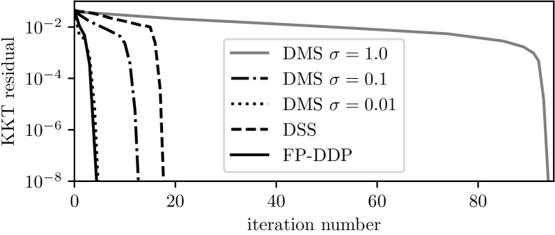
Figure 1: KKT residuals for DMS with penalty parameter $\sigma\in\{1.0,0.1,0.01\}$, DSS, and FP-DDP.

Fig. 1 shows the convergence of the different methods. Looking at the iteration numbers reveals that FP-DDP takes 5 iterations to converge to a feasible solution. Interestingly, always full steps are taken. DSS takes 18 iterations until the optimal solution is found. Since the underlying system is highly unstable the open-loop forward simulation in DSS yields trajectories that are far from the solution. This results in smaller steps for DSS and therefore slower convergence. Looking at DMS reveals that the choice of the penalty parameter highly influences the convergence speed. Setting the initial penalty parameter $\sigma=1$ as in [4] achieves convergence in 94 iterations. The Maratos effect seems to be taking place whereas taking an initial penalty parameter of $0.01$ yields convergence within 5 iterations. This demonstrates the dependence of merit-function-based algorithms on their penalty parameter whereas FP-DDP does not require this parameter choice.

V-C Free-Time P2P Motion of Cart Pendulum with Obstacle

In this section, a free-time cart pendulum problem with obstacle avoidance is discussed. The system dynamics and parameters are given in [19]. The states $x=(p,v,\theta,\omega)^{\top}\in\mathbb{R}^{4}$ consist of position, velocity, pole angle, and pole angular velocity. The control (force) inputs are given by $u=F\in\mathbb{R}$. The free-time $T$ is modeled as an additional state using time scaling. The task is to move from an initial upward pole position corresponding to $\bar{x}_{1}=(0,0,0,0)^{\top}$ to the final upward position $\bar{x}_{N+1}=(5.0,0,0,0)^{\top}$. In addition, some bound constraints on the states, i.e., $\underline{x}=(-1.0,-2.0,-\frac{\pi}{4},-0.5)$, $\bar{x}=(6.0,2.0,\frac{\pi}{4},0.5)$, $\underline{x}\leq x_{i}\leq\bar{x}$ with $i=2,\ldots,N$, as well as $|u_{i}|\leq 5.0$ for $i=1,\ldots,N$ are imposed. During the motion, the endpoint of the pole has to avoid a circular obstacle with its center at $(\tilde{p},0.9)^{\top}$, $\tilde{p}\in\mathbb{R}$ and having a radius of $0.3$. The horizontal position of the center of the obstacle is chosen from $100$ linearly spaced values between $0.7$ and $4.3$, i.e., in total, $100$ problems are solved.

FP-DDP is compared against the state-of-the-art solver IPOPT [21] which solves the same problem formulation as FP-DPP and against scipy.optimize.minimize using a Truncated-Newton method [17], [20] and solving the unconstrained NLP of SEQUOIA which is given in Table I. IPOPT is used through its CasADi interface which provides the derivative information. The derivatives for the unconstrained NLP were manually built in CasADi and then passed to scipy.optimize.minimize. As Hessian, the GGN matrix was used. IPOPT used exact Hessian information. The solvers were initialized with a constant trajectory at the initial position. The time is initialized with the constant value $T=5.0$.

To compare the different algorithms, the Dolan and Moré performance profiles [8] were used. As the performance metric the number of Hessian evaluations was chosen. Fig. 2 shows the results of the different solvers. The vertical axis $\rho_{s}(\tau)$ indicates what fraction of all test problems were solved. The horizontal axis $\tau$ indicates that the solver was not more than $\tau$ times worse than the best solver. If the performance of an algorithm is better relative to another algorithm, this is indicated by higher values of $\rho_{s}(\tau)$.

.

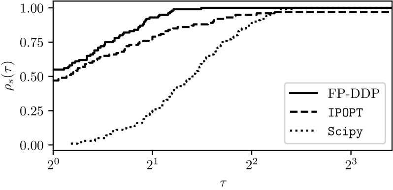
Figure 2: Performance plot of Hessian evaluations for FP-DDP, IPOPT, and truncated Newton Scipy.

It can be seen that FP-DDP outperforms the other algorithms and is in almost 55% of the cases the algorithm with the least amount of Hessian evaluations until convergence is achieved. IPOPT fails once in the restoration phase. Apart from that all solvers are robust and can solve the test problems, but overall FP-DDP converges the fastest. This indicates the strong performance of the proposed algorithm. An additional advantage of FP-DDP is that it can be efficiently implemented using high-performance linear algebra packages such as BLASFEO [11] yielding fast execution times.

VI Conclusion

This paper introduced an efficient algorithm for finding feasible trajectories in direct optimal control based on DDP and an Armijo-type line search. Theoretical convergence guarantees were derived and the efficiency of the algorithm was demonstrated against state-of-the-art methods. Possible future research areas include an efficient C implementation of the algorithm and its embedding into an OCP NLP solver.

References

- [1] J. Andersson, J. Gillis, G. Horn, J. Rawlings, and M. Diehl. CasADi – a software framework for nonlinear optimization and optimal control. Math. Program. Comput., 11(1):1–36, 2019.
- [2] K. Baumgärtner, F. Messerer, and M. Diehl. A unified local convergence analysis of differential dynamic programming, direct single shooting, and direct multiple shooting. In Proc. European Control Conference (ECC), 2023.
- [3] E. Bergou, Y. Diouane, and V. Kungurtsev. Convergence and complexity analysis of a levenberg–marquardt algorithm for inverse problems. J. Optim. Theory Appl., 185, 06 2020.
- [4] R. Byrd, G. Lopez-Calva, and J. Nocedal. A line search exact penalty method using steering rules. Math. Program., 133:1–35, 01 2009.
- [5] H. Chen and F. Allgoẅer. A quasi-infinite horizon nonlinear model predictive control scheme with guaranteed stability. Automatica, 34(10):1205–1217, 1998.
- [6] Murray D. and Yakowitz S. Differential dynamic programming and newton’s method for discrete optimal control problems. J. Optim. Theory Appl., 43:395–414, 1984.
- [7] M. Diehl. Lecture Notes on Numerical Optimization. 2016.
- [8] Elizabeth Dolan and Jorge Moré. Benchmarking optimization software with performance profiles. Math. Program., 91, 03 2001.
- [9] R. Fletcher and S. Leyffer. Nonlinear programming without a penalty function. Math. Program., 91:239–269, 02 1999.
- [10] G. Frison and M. Diehl. HPIPM: a high-performance quadratic programming framework for model predictive control. In Proc. IFAC World Congress, Berlin, Germany, July 2020.
- [11] G. Frison, D. Kouzoupis, T. Sartor, A. Zanelli, and M. Diehl. BLASFEO: Basic linear algebra subroutines for embedded optimization. ACM Trans. Math. Softw. (TOMS), 44(4):42:1–42:30, 2018.
- [12] J. Gillis, B. Vandewal, G. Pipeleers, and J. Swevers. Effortless modeling of optimal control problems with rockit. In Proc. 39th Benelux Meet. Sys. Cont., Elspeet, the Netherlands, July 2020.
- [13] Michael Hintermüller. Semismooth newton methods and applications. Department of Mathematics, Humboldt-University of Berlin, 2010.
- [14] C. Mastalli et al. Crocoddyl: An efficient and versatile framework for multi-contact optimal control. 2020 IEEE International Conference on Robotics and Automation (ICRA), 2019.
- [15] D. Mayne. A second-order gradient method for determining optimal trajectories of non-linear discrete-time systems. Int. J. Control, 3(1):85–95, 1966.
- [16] L. Nita and E. Carrigan. SEQUOIA: A sequential algorithm providing feasibility guarantees for constrained optimization. In Proc. IFAC World Congress, Yokohama, Japan, 2023.
- [17] J. Nocedal and S. J. Wright. Numerical Optimization. Springer Series in Operations Research and Financial Engineering. Springer, 2 edition, 2006.
- [18] M. Tenny, S. Wright, and J. Rawlings. Nonlinear model predictive control via feasibility-perturbed sequential quadratic programming. Comput. Optim. Appl., 28:87–121, 2004.
- [19] R. Verschueren, N. van Duijkeren, R. Quirynen, and M. Diehl. Exploiting convexity in direct optimal control: a sequential convex quadratic programming method. In Proc. IEEE Conference Decision and Control (CDC), 2016.
- [20] P. Virtanen et al. SciPy 1.0: Fundamental Algorithms for Scientific Computing in Python. Nature Methods, 17:261–272, 2020.
- [21] A. Wächter and L. Biegler. On the implementation of an interior-point filter line-search algorithm for large-scale nonlinear programming. Math. Program., 106(1):25–57, 2006.
- [22] S. Wright and M. Tenny. A feasible trust-region sequential quadratic programming algorithm. SIAM J. Optim., 14:1074–1105, 1 2004.
- [23] S. Yakowitz and B. Rutherford. Computational aspects of discrete-time optimal control. Appl. Math. Comp., 15(1):29–45, 1984.
- [24] J. Zhou and A. Tits. User’s guide for FSQP version 3.0c: A FORTRAN code for solving constrained nonlinear (minimax) optimization problems, generating iterates satisfying all inequality and linear constraints. 01 1992.