Single- and Multi-Agent Private Active Sensing:
A Deep Neuroevolution Approach

Abstract

In this paper, we focus on one centralized and one decentralized problem of active hypothesis testing in the presence of an eavesdropper. For the centralized problem including a single legitimate agent, we present a new framework based on NeuroEvolution (NE), whereas, for the decentralized problem, we develop a novel NE-based method for solving collaborative multi-agent tasks, which interestingly maintains all computational benefits of single-agent NE. The superiority of the proposed EAHT approaches over conventional active hypothesis testing policies, as well as learning-based methods, is validated through numerical investigations in an example use case of anomaly detection over wireless sensor networks.

I Introduction

Active Hypothesis Testing (AHT) refers to the family of problems where one legitimate agent or decision maker, or a group of collaborating agents or decision makers, adaptively select(s) sensing actions and collect(s) observations in order to infer the underlying true hypothesis in a fast and reliable manner [1, 2]. AHT and related problems, such as active parameter estimation [3] and active change point detection [4, 5], find numerous applications in wireless communications, including anomaly detection over sensor networks [6], strong or weak radar models for target detection [7], cyber-intrusion detection, target search, and adaptive beamforming [8], as well as, very recently, RIS-enabled localization [9] and channel estimation [10]. In addition, AHT is closely related to the feedback channel coding problem [11].

In [12, 13, 14, 15], AHT was modeled as a Partially-Observable Markov Decision Process (POMDP). In particular, [13, 14, 15] showcased the superiority of Deep Reinforcement Learning (DRL) strategies over conventional AHT heuristics. The recurrent DRL algorithm in [13] was shown to compete with classical model-based strategies without having knowledge of the environment dynamics. More complex AHT-based anomaly detection problems with sampling costs were discussed in [16], and appropriate DRL strategies that balance detection objectives with cost management were proposed. Collaborative multi-agent DRL for AHT was studied in [17, 18, 19]. Specifically, the authors in [19] discussed how sampling cost constraints can be managed in a multi-agent environment using Lagrange multipliers. Very recently, AHT in the presence of adversaries that target to corrupt the observations of legitimate agents was studied in [20, 21]. The former work assumed non-adaptive decision making where the agent terminates when an adversary is detected, while the latter work focused on the case of adaptive and intelligent legitimate as well as adversarial agents.

Due to the growing concerns for data privacy, many works studied privacy in passive hypothesis testing problems, where there is no control over the sensing actions. For example, [22] elaborated on how to perform remote estimation of the system state through sensor data while impairing the filtering ability of eavesdroppers, and [23] studied secure distributed hypothesis testing. The problem of single-agent Evasive AHT (EAHT), where a passive Eavesdropper (Eve) collects noisy estimates of the legit observations and tries to infer the underlying hypothesis, was studied in [24], focusing however explicitly on the asymptotical case. In that work, the authors formulated single-agent EAHT as a constrained optimization problem including the legitimate agent’s and the Eavesdropper’s (Eve) error exponent. However, near-optimal or optimal action selection policies were not presented. In this paper, motivated by the lack of explicit policies for EAHT, we present novel single- and multi-agent EAHT approaches for wireless sensor networks that are based on a deep NeuroEvolution (NE) framework. Our contributions are summarized as follows:

1. We formulate the single-agent EAHT problem studied in [24] as a constrained POMDP and present a NE-based method for solving it. Our numerical investigations showcase that our method satisfies the privacy constraint, while achieving similar accuracy to popular AHT methods that ignore the existence of any adversary.

2. We present a novel formulation of the decentralized multi-agent EAHT problem, where a group of agents tries to infer the underlying hypothesis, while keeping it hidden from a passive eavesdropper.

3. We present a novel method for solving decentralized POMDPs via deep NE, and apply it to the decentralized EAHT problem at hand. We numerically compare this scheme with state-of-the-art multi-agent DRL algorithms. It is demonstrated that our NE-based method outperforms existing algorithms, while maintaining all computational benefits of single-agent NE.

II EAHT Problem Formulations

In this section, we introduce two EAHT problems, a centralized one with a single agent and a decentralized one with a group of agents having access to different sensing action sets. In the latter problem, the agents exchange information with each other and each one separately infers the hypothesis [17].

II-A Centralized Problem

Let $\mathcal{X}\triangleq\{0,1,2,\ldots,|\mathcal{X}|-1\}$ be a finite set of hypotheses, while the true hypothesis $x$ is unknown. A legitimate agent has access to a finite set of sensing actions $\mathcal{A}$, and at each time instance $t$, it selects an action $a_{t}\in\mathcal{A}$. In response to this action, the agent collects the noisy observation $y_{t}$. In parallel, an eavesdropper (Eve) being present in the system receives another noisy observation $z_{t}$. The conditional probability of $y_{t}$ given $x$ and $a_{t}$ is denoted as $P[y_{t}|a_{t},x]$, whereas the respective conditional probability of $z_{t}$ is $Q[z_{t}|a_{t},x]$. We assume that the distributions $P[\cdot]$ and $Q[\cdot]$ are either known a priori [12, 24] or can be reliably estimated from a large dataset. The known prior probability over the hypotheses is denoted as $\pi_{0}(x)$.

The legitimate agent maintains an $|\mathcal{X}|$-dimensional belief vector $\pi^{L}_{t}(\mathcal{X})$ over all possible hypotheses $x\in\mathcal{X}$ at time instant $t$, and Eve does the same via the belief vector $\pi^{E}_{t}(\mathcal{X})$. For the former, given an action observation pair $(a_{t},y_{t})$, the legit belief on each hypothesis $x$ is updated as follows [15]:

$$\pi^{L}_{t+1}(x)=\frac{\pi^{L}_{t}(x)P[y_{t}|a_{t},x]}{\sum_{x^{\prime}\in\mathcal{X}}\pi^{L}_{t}(x^{\prime})P[y_{t}|a_{t},x^{\prime}]}.$$ (1)

Similarly, Eve’s belief given a pair $(a_{t},z_{t})$ can be updated as:

$$\pi^{E}_{t+1}(x)=\frac{\pi^{E}_{t}(x)Q[z_{t}|a_{t},x]}{\sum_{x^{\prime}\in\mathcal{X}}\pi^{E}_{t}(x^{\prime})Q[z_{t}|a_{t},x]}.$$ (2)

The posterior error probability of the agent at each time instant $t$ is obtained as $\gamma^{L}_{t}=1-\max_{x\in\mathcal{X}}\pi^{L}_{t}(x)$, while for Eve as $\gamma^{E}_{t}=1-\max_{x\in\mathcal{X}}\pi^{E}_{t}(x)$. We also assume that the legitimate agent controls the stopping time $\tau$. To this end, once the episode terminates, both the agent and Eve guess the underlying hypothesis according to the maximum a posteriori decoding rule.

The goal of the legitimate agent is to reliably estimate the true hypothesis as quickly as possible, while keeping Eve’s error probability above a certain application/agent-defined threshold. Let $g_{t}\triangleq g(a_{t}|\pi^{L}_{t}(\mathcal{X}))$ represent the policy of the agent at each time instance $t$. The policy is a probabilistic mapping from belief vectors to the action set combined with an additional action for episode termination. The total policy of the legitimate agent for a sensing horizon of $\tau$ time slots is defined as follows:

$${\rm g}\triangleq(g_{1},g_{2}\cdots,g_{\tau},\tau).$$ (3)

By using user defined scalars $E$ and $L$, this problem can be formulated as a constrained POMDP problem as follows:

$$\mathcal{OP}_{1} :\underset{{\rm g}}{\min}\,\,E[\tau]$$

$$\quad\text{\text{s}.\text{t}.}\,\,\,\,\,\gamma^{L}_{\tau}\leq L,\,\,\gamma^{E}_{t}\geq E\,\,\forall t=1,2,\ldots,\tau.$$

The expectation in the latter objective is taken with respect to ${\rm g}$, $P[\cdot]$, $Q[\cdot]$, and $\pi_{0}(x)$. It is noted that, without the second constraint, $\mathcal{OP}_{1}$ is essentially an AHT problem. Even without the instantaneous constrains, POMDPs are NP-hard [25], therefore, we do not expect to find exact solutions. In the next section, we will present near-optimal policies using deep policy optimization techniques.

II-B Decentralized Problem

In the decentralized problem, a group of $K$ legitimate agents collaborates to infer the underlying hypothesis. We assume that each $k$-th agent, with $k=1,2,\ldots,K$, has access to a sensing action set $\mathcal{A}^{k}$. By probing the environment with an action $a^{k}_{t}$ at time slot $t$, the $k$-th agent receives a noisy observation $y_{t}^{k}$ with conditional distribution $P[y_{t}^{k}|a_{t}^{k},x]$, while Eve observes the noisy quantity $z_{t}^{k}$ with conditional distribution $Q[z_{t}^{k}|a_{t}^{k},x]$. It is assumed that both $y_{t}^{k}$ and $z_{t}^{k}$ do not depend on the actions of other than the $k$-th agent. This agent is assumed to also broadcast the action and observation tuple $(a_{t}^{k},y_{t}^{k})$ to a set $\mathcal{O}^{k}$ of neighboring legitimate agents, while receiving observations from another set $\mathcal{I}^{k}$ of agents.

Given a pair $({\rm a}_{t},{\rm y}_{t})$ of actions and observations, with ${\rm a}_{t}\triangleq(a_{t}^{1},a_{t}^{2},\ldots,a_{t}^{K})$ and ${\rm y}_{t}\triangleq(y_{t}^{1},y_{t}^{2},\ldots,y_{t}^{K})$, each $k$-th legitimate agent updates its belief according to the expression:

$$\rho_{t}^{k}(x)=\frac{\rho_{t-1}^{k}(x)\prod_{(a_{t}^{k},y_{t}^{k})\in(\rm a_{t},\rm y_{t})}P[y_{t}^{k}|a_{t}^{k},x]}{\sum_{x^{\prime}\in\mathcal{X}}\rho_{t-1}^{k}(x^{\prime})\prod_{(a_{t}^{k},y_{t}^{k})\in(\rm a_{t},\rm y_{t})}P[y_{t}^{k}|a_{t}^{k},x^{\prime}]}.$$ (4)

Similarly does Eve via the following belief update rule:

$$\rho_{t}^{E}(x)=\frac{\rho_{t-1}^{E}(x)\prod_{(a_{t}^{k},z_{t}^{k})\in(\rm a_{t},\rm z_{t})}Q[z_{t}^{k}|a^{k}_{t},x]}{\sum_{x^{\prime}\in\mathcal{X}}\rho_{t-1}^{E}(x^{\prime})\prod_{(a_{t}^{k},z_{t}^{k})\in(\rm a_{t},\rm z_{t})}Q[z_{t}^{k}|a^{k}_{t},x]},$$ (5)

where ${\rm z}_{t}\triangleq(z_{t}^{1},z_{t}^{2},\ldots,z_{t}^{K})$.

In this multi-agent case, we will further assume that each of the action sets $A^{k}$ also contains a “no sensing action” element, according to which the observations $y_{t}^{k}$ and $z_{t}^{k}$ are not generated. It is noted, however, that when a $k$-th legitimate agent selects this option, it can still update it’s belief using information from the other $K-1$ agents. We also consider that each agent can exit independently the sensing process, therefore, their communication graph may vary with time. To treat this general case, we consider as stopping time the time instance the last agent exits the sensing process, i.e., $\tau=\max_{k}\tau_{k}$ with $\tau_{k}$ denoting the stopping time of each $k$-th agent. We also use notation $\gamma_{t,k}^{L}$ for the posterior error probability of each agent $k$ at time instant $t$. Similar to $\mathcal{OP}_{1}$, our goal is to find a collective agent policy ${\rm g}^{C}\triangleq({\rm g}_{1},{\rm g}_{2},\ldots,{\rm g}_{k})$, where each ${\rm g}_{k}$ is obtained from (3), that approximately solves the following optimization problem.

$$\mathcal{OP}_{2} :\underset{{\rm g}^{C}}{\min}\,\,E[\tau]$$

$$\quad\text{\text{s}.\text{t}.}\,\,\,\,\,\gamma_{\tau_{k},k}^{L}\leq L\,\,\forall k,\,\,\gamma^{E}_{t}\geq E\,\,\forall t=1,2,\ldots,\tau.$$

III Deep Neuroevolution Schemes for EAHT

The consideration of NE schemes for solving MDPs and POMDPs is an old idea, dating back, for example, to [26, 27], which has been left largely undeployed, mainly due to the recent impressive success of DRL approaches. However, in the past few years, it has been experimentally shown that, even simple NE schemes, can rival back-propagation algorithms, such as Q-learning and policy gradients, outperforming DRL approaches in various single-agent POMDPs [28, 29]. The main benefits of NE over DRL are summarized as follows:

• NE is easier to implement (replay buffers, advantage estimation etc. are not needed) and to parallelize over multiple Central Processing Units (CPUs).

• Reward reshaping and exploration techniques are not required in NE schemes.

• DRL schemes face instability problems, which are associated with back-propagation through time. This issue is absent in NE.

NE’s basic idea is to directly search the space of the policy networks via nature-inspired algorithms; note that, in NE, critic networks are not considered. In particular, each chromosome of an individual represents some parameters of a policy neural network [28, 30]. It is noted that, due to the large number of parameters in a network, it is typically infeasible to construct individuals representing all of the network parameters. To this end, techniques that take advantage of the neural network structure in order to construct smaller individuals are usually devised. Particularly, a generation of individuals is initialized randomly. Each individual is then evaluated, and its fitness function is stored. The individuals with the highest fitness function are selected for mating. During mating, the parameters of two or more individuals are merged by various methods (e.g., crossover operation). The new individuals then replace the ”weaker” individuals of the population. This procedure is repeated for multiple generations. It is noted that further genetic operations [31], such as mutation, can be utilized to increase exploration.

In the following, we will describe how NE can be applied to the considered centralized EAHT problem. In addition, a novel NE method to deal with multi-agent POMDPs will be presented, which will be deployed to solve the considered decentralized EAHT problem.

III-A Centralized EAHT

The policy network of an individual, which is needed in the NE formulation, is a mapping from beliefs to actions. We will use the Cooperative Synapse NE (CoSyNE) method [30] to evolve a feed-forward policy network. The fitness function of a policy network $\theta$ is defined as follows:

$$f(\theta)=\begin{cases}-A_{E},\quad A_{E}\geq 1-E\\ \hat{E}_{\tau}^{-1},\quad\,\,\,\text{otherwise}\end{cases},$$ (6)

where $A_{E}\triangleq\hat{E}\max_{t}\max_{x}\pi_{t}^{E}(x)$ represents the average of the maximum Eve’s belief value during an episode with $\hat{E}$ being the sample average, and $\hat{E}_{\tau}$ is the average horizon, both calculated from a large number $EP$ of Monte Carlo episodes. It is noted that episodes in which Eve has large beliefs on some hypothesis are penalized. According to this definition, if a policy network cannot satisfy the privacy constraint, it is “encouraged” to do so; this is imposed from the first part of the fitness function $f(\theta)$. Otherwise, the network is “encouraged” to minimize the expected stopping time. Finally, individuals that satisfy the privacy constraint with the shortest stopping time are selected for mating.

Similar to recent works on deep learning for active hypothesis testing and related problems, e.g., [14, 19], the policy network is only responsible for action selection. In this paper, we utilize a simple stopping rule, according to which termination takes place the first time $t$ for which holds $\gamma_{t}^{L}<L$.

III-B Decentralized EAHT

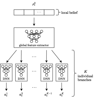
Figure 1: The proposed neural network architecture for NE-based multi-agent cooperation. Each agent passes its belief to the global feature extractor, and then, to its individual branch. The entire architecture can be evolved with typical NE algorithms, such as the CoSyNE one [30] deployed in this paper.

In this section, we design a dual-component deep NE approach for multi-agent cooperative tasks, which builds upon existing single-agent NE algorithms; to this end, we will use the previously mentioned CoSyNE algorithm [30], but other algorithms can be used as well. The proposed approach maintains all the previously highlighted NE benefits, and can be applied to tasks with multiple heterogeneous agents. Its first component is a feature extractor network that is utilized by all agents, and its second component is comprised of $K$ individual branches, one for each agent. The idea is to deploy the feature extractor weights to learn functions that will be used by all agents. The individual branches are then used to learn specific policies for each agent. Since the agents are heterogeneous, they might have vastly different beliefs and action sets of different sizes. Moreover, some agents may have to remain inactive more often because their actions cause very significant information leakage. For the latter reasons, the proposed approach uses individual branches. The entire architecture is evolved as one network using CoSyNE [30]. During the deployment/testing phase, each agent is provided with the common feature extractor and its individual branch. The proposed neural network architecture for NE-based multi-agent cooperative tasks is illustrated in Fig. 1.

In the proposed decentralized EAHT scheme, the fitness function of an individual is evaluated as follows. For each evaluation episode, the hypothesis is randomly sampled from $\pi_{0}(\mathcal{X})$ and the beliefs of all agents are initialized. At each time instance, each agent selects its action by passing the local belief through the feature extractor, and then, by forwarding the resulting output to its local branch. After $EP$ Monte Carlo episodes take place, the fitness is computed according to expression (6), considering an appropriate adjustment to account for the decentralized stopping time, as defined in Section II-B. Each agent utilizes the stopping rule $\gamma_{t}^{L}<L$, as defined in the previous Section III-A.

IV Numerical Results and Discussion

In this section, we present performance evaluation results for our NE-based single- and multi-agent EAHT schemes considering an anomaly detection scenario over wireless sensor networks. Different values for the thresholds $L$ and $E$ as well as for the number of sensors have been considered.

TABLE I: Flipping probabilities for each sensor’s three distinct access actions.

Sensor Access Action Number	$f^{L}$	$f^{E}$
1	0.125	0.125
2	0.2	0.4
3	0.25	0.45

IV-A NE Implementation

The proposed single-agent NE scheme uses a feed-forward neural network with $2$ hidden layers each comprising $200$ units, whereas the proposed multi-agent algorithm utilizes a feature extractor with $2$ hidden layers of $300$ hidden units and $K$ branches (each corresponding to one of the $K$ agents) with $2$ layers of $200$ units.

IV-B Single-Agent EAHT

We consider $S$ independent and identical sensors with the task to detect anomalies in their proximity [14]. It is assumed that any number of sensors can be near an anomaly, therefore there are in total $2^{S}$ possible hypotheses. At each time instance, the single agent probes one sensor and receives the following binary observation:

$$y_{t}=\begin{cases}s,\quad\quad\,\,\,\,\text{with probability }1-f^{L}\\ 1-s,\quad\text{with probability}f^{L}\\ \end{cases},$$ (7)

where $s$ is a binary number corresponding to the sensor’s state (whether it is near an anomaly or not) and $f^{L}$ is the flipping probability. A similar equation holds for the Eve’s observation $z_{t}$, whose a flipping probability is denoted by $f^{E}$. We assume that the single agent can access each sensor with three different actions, each corresponding to one of the three different flipping probability values. Therefore, the total actions available to the agent are $3S$. The three different flipping probability values and the respective three distinct sensor access actions are demonstrated in Table I.

In the performance results illustrated in Figs. 2–4, we have set $L=0.1$ and considered two values for $E$, namely $E=0.4$ and $0.3$. In addition, the number of available sensors $S$ was varied between $2$ to $4$. Finally, the fitness evaluation episodes number was set to $EP=1000$. As benchmark schemes, we have implemented two conventional AHT strategies that ignore the the existence of Eve: the Chernoff test [1] and a myopic Extrinsic Jensen-Shannon (EJS) maximization strategy [15]. We have also simulated the performance of a Proximal Policy Optimization (PPO) DRL algorithm rewarded for error minimization, like the one in [19, 13]. For this case, if the privacy constraint failed, a large penalty was reached, and consequently, the episode was terminated. In this DRL approach, larger networks than the proposed NE-based schemes were used, in particular, an actor and a critic with $2$ hidden layers each consisting of $300$ units. It is noted that a plethora of alternative reward functions were also studied, without, however, yielding any performance improvement. Details on this investigation will be available in a future extended version of this work.

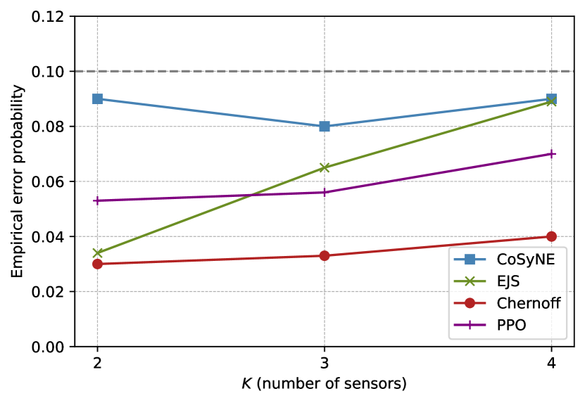
(a) $E=0.3$

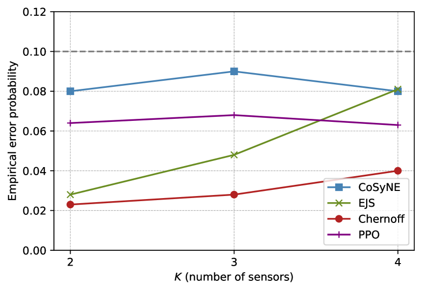
(b) $E=0.4$

Figure 2: Legitimate error probability of single-agent EAHT for different values of the threshold $E$.

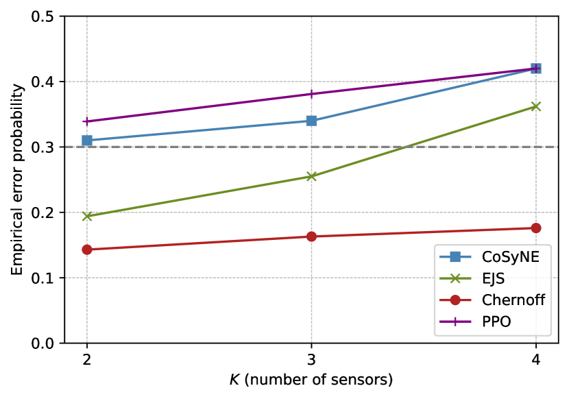
(a) $E=0.3$

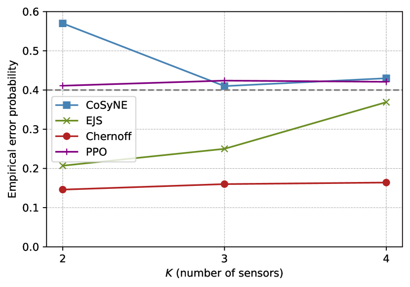
(b) $E=0.4$

Figure 3: Eavesdropping error probability of single-agent EAHT for different values of the threshold $E$.

The average stopping time, the legitimate empirical error probability (at the final time instance), and the empirical error probability of Eve after training demonstrated in Figs. 2–4 were obtained via $EP=1000$ Monte Carlo simulations. It can be first observed that the legitimate error probability is smaller than the value of the threshold $L$ for all approaches. Interestingly, the proposed NE-based EAHT approach and the PPO benchmark lead to substantially higher error probability on Eve’s side. However, the conventional approaches cannot satisfy the privacy constraints, resulting in a large margin from the latter best schemes. It can be also seen that Eve’s error probability is always less than $0.3$. In addition, for some experiments, Eve’s error probability is more than $50\%$ smaller than the desired threshold. As expected, there is some trade-off in the episode stopping time, since the proposed NE and PPO methods need to perform a few more sensing actions. It is finally shown that the CoSyNE algorithm achieves a shorter average stopping time than the PPO benchmark, in all simulated investigations. In fact, in most of the simulations’ settings, the stopping time of the CoSyNE algorithm was at least 20 $\%$ shorter than the stopping time with PPO. Moreover, CoSyNE terminates faster than the Chernoff test which by design ignores the existence of any adversary.

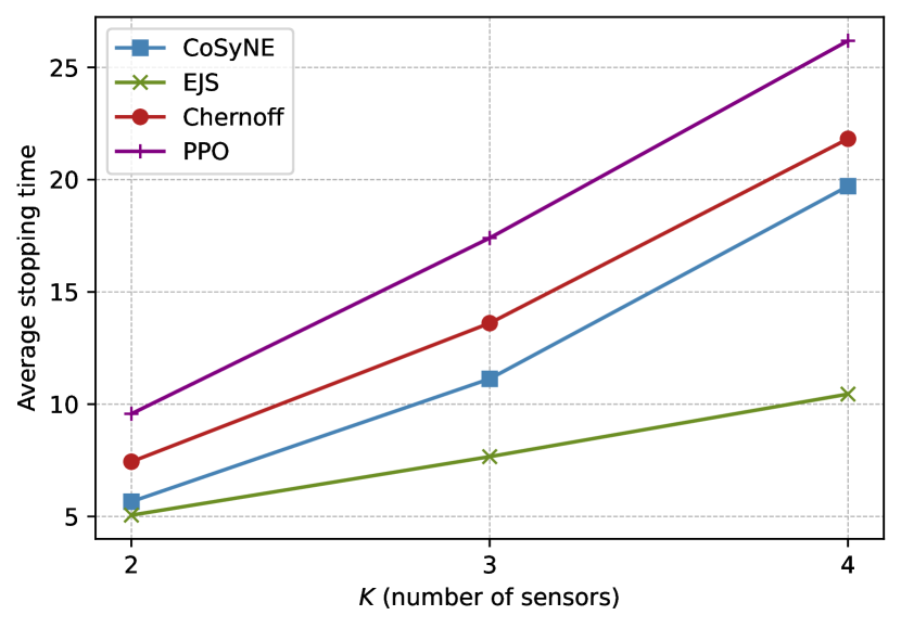
(a) $E=0.3$

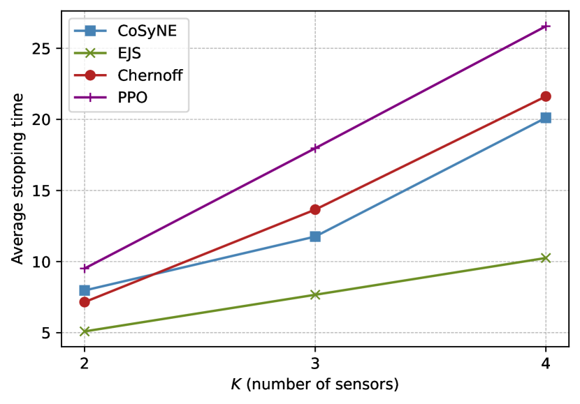
(b) $E=0.4$

Figure 4: Average episode stopping time of single-agent EAHT for different values of the threshold $E$.

IV-C Multi-Agent EAHT

Due to the decentralized nature of this EAHT problem, we have only considered one DRL-based benchmark, and specifically, a multi-agent PPO algorithm with separate actors for each agent and a global critic, similar to [17, 19]. For this benchmark’s implementation, when the privacy constraint was satisfied, it was rewarded for error minimization, otherwise, a large penalty was received. Besides the penalty, training was nearly identical to state-of-the-art DRL approaches for multi-agent active sensing [17, 19]. In terms of implementation complexity, this PPO-based benchmark tailored to individual actors deploys a neural network with $2$ hidden layers, each comprising $300$ units, and a global critic with $3$ hidden layers, each of $300$ units.

In Fig. 5, we considered the same observation model with the single-agent case as well as $K=4$ fully connected agents, fixed the thresholds as $L=0.1$ and $E=0.3$, and varied the number of sensors $S$ from $6$ to $12$, yielding $2^{12}$ possible hypotheses in total. We have assumed that the first two agents have access to the first half of the sensors, and the other two have access to the rest. Since both our NE-based and the DRL benchmark for multi-agent EAHT approaches satisfy the accuracy and privacy constraints, we only include a plot of the average stopping time. Interestingly, the NE approach achieves a shorter stopping time for larger values of $K$.

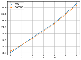
Figure 5: Average episode stopping times of multi-agent EAHT for the threshold values $L=0.1$ and $E=0.3$.

V Conclusion and future work

In this paper, we studied both single- and multi-agent EAHT problems and presented NE-based solutions. Specifically for the decentralized multi-agent problem, we devised a novel NE method for dealing with collaborative multi-agent tasks, which maintains all computational benefits of single-agent NE. The superiority of the presented approaches over EAHT benchmarks was demonstrated through numerical simulations.

There are a lot of exiting directions for future work, as extensions of the presented NE-based framework in this paper. One direction is to extend our experimental investigations and the theoretical analysis of [24] to other challenging active sensing tasks, e.g., similar to [3, 5, 8]. It is also worthwhile to examine scenarios with multiple heterogeneous and active eavesdroppers. Finally, we believe that our proposed decentralized NE-based approach can be applied to more collaborative decision making tasks beyond hypothesis testing, e.g., robotic agents [32], resource allocation for the internet-of-things [33], and role allocation in crisis management [34].

References

- [1] H. Chernoff, “Sequential design of experiments,” Ann. Math. Stat., vol. 30, no. 3, pp. 755–770, 1959.
- [2] S. Nitinawarat, G. Atia, and V. V. Veeravalli, “Controlled sensing for multihypothesis testing,” IEEE Trans. Autom. Control, vol. 58, no. 10, pp. 2451–2464, 2013.
- [3] A. Mukherjee, A. Tajer, P.-Y. Chen, and P. Das, “Active sampling of multiple sources for sequential estimation,” IEEE Trans. Signal Process, vol. 70, pp. 4571–4585, 2022.
- [4] G. Fellouris and V. V. Veeravalli, “Quickest change detection with controlled sensing,” in Proc. IEEE ISIT, pp. 1921–1926, 2022.
- [5] A. Gopalan, B. Lakshminarayanan, and V. Saligrama, “Bandit quickest changepoint detection,” in Proc. NeurIPS, 2021.
- [6] K. Cohen and Q. Zhao, “Active hypothesis testing for anomaly detection,” IEEE Trans. Inf. Theory, vol. 61, no. 3, pp. 1432–1450, 2015.
- [7] M. Franceschetti, S. Marano, and V. Matta, “Chernoff test for strong-or-weak radar models,” IEEE Trans. Signal Process, vol. 65, no. 2, pp. 289–302, 2017.
- [8] F. Sohrabi, Z. Chen, and W. Yu, “Deep active learning approach to adaptive beamforming for mmwave initial alignment,” in Proc. IEEE ICASSP, 2021.
- [9] Z. Zhang, T. Jiang, and W. Yu, “Active sensing for localization with reconfigurable intelligent surface,” 2023, arXiv:2312.09002.
- [10] F. Sohrabi, T. Jiang, W. Cui, and W. Yu, “Active sensing for communications by learning,” IEEE J. Sel. Areas Commun, vol. 40, no. 6, pp. 1780–1794, 2022.
- [11] Y. Polyanskiy and Y. Wu, “Lecture notes on information theory,” tech. rep., 2019.
- [12] M. Naghshvar and T. Javidi, “Active sequential hypothesis testing,” Ann. Stat., vol. 41, dec 2013.
- [13] G. Stamatelis and N. Kalouptsidis, “Active hypothesis testing in unknown environments using recurrent neural networks and model free reinforcement learning,” in Proc EUSIPCO, 2023.
- [14] C. Zhong, M. C. Gursoy, and S. Velipasalar, “Deep actor-critic reinforcement learning for anomaly detection,” in Proc. IEEE GLOBECOM, 2019.
- [15] D. Kartik, E. Sabir, U. Mitra, and P. Natarajan, “Policy design for active sequential hypothesis testing using deep learning,” in Proc. Allerton, 2018.
- [16] C. Zhong, M. C. Gursoy, and S. Velipasalar, “Controlled sensing and anomaly detection via soft actor-critic reinforcement learning,” in Proc. IEEE ICASSP, 2022.
- [17] H. Szostak and K. Cohen, “Decentralized anomaly detection via deep multi-agent reinforcement learning,” in Proc. Allerton, 2022.
- [18] G. Joseph, C. Zhong, M. C. Gursoy, S. Velipasalar, and P. K. Varshney, “Scalable and decentralized algorithms for anomaly detection via learning-based controlled sensing,” IEEE Trans. Signal Inf. Process. Netw., vol. 9, pp. 640–654, 2023.
- [19] G. Stamatelis and N. Kalouptsidis, “Deep reinforcement learning for active hypothesis testing with heterogeneous agents and cost constraints,” TechRxiv, May 2023.
- [20] M.-C. Chang, S.-Y. Wang, and M. R. Bloch, “Controlled sensing with corrupted commands,” in Proc. Allerton, 2022.
- [21] N. Kalouptsidis and G. Stamatelis, “Deep reinforcement learning and adaptive strategies for adversarial active hypothesis testing,” under review, 2022.
- [22] A. Tsiamis, K. Gatsis, and G. J. Pappas, “State estimation with secrecy against eavesdroppers,” IFAC-PapersOnLine, vol. 50, no. 1, pp. 8385–8392, 2017. 20th IFAC World Congress.
- [23] M. Mhanna and P. Piantanida, “On secure distributed hypothesis testing,” in Proc. IEEE ISIT, 2015.
- [24] M.-C. Chang and M. R. Bloch, “Evasive active hypothesis testing,” IEEE J. Sel. Areas Inf. Theory, vol. 2, no. 2, pp. 735–746, 2021.
- [25] C. H. Papadimitriou and J. N. Tsitsiklis, “The complexity of markov decision processes,” Math. Oper. Res., vol. 12, pp. 441–450, 1987.
- [26] D. E. Moriarty and R. Miikkulainen, “Efficient reinforcement learning through symbiotic evolution,” Machine Learning, no. AI94-224, pp. 11–32, 1996.
- [27] F. J. Gomez and J. Schmidhuber, “Co-evolving recurrent neurons learn deep memory POMDPs,” in Proc. GECCO, 2005.
- [28] T. Salimans, J. Ho, X. Chen, S. Sidor, and I. Sutskever, “Evolution strategies as a scalable alternative to reinforcement learning,” arXiv:1703.03864, 2017.
- [29] P. Chrabaszcz, I. Loshchilov, and F. Hutter, “Back to basics: Benchmarking canonical evolution strategies for playing atari,” in Proc. IJCAI, 2018.
- [30] F. Gomez, J. Schmidhuber, and R. Miikkulainen, “Accelerated neural evolution through cooperatively coevolved synapses,” JMLR, vol. 9, no. 31, pp. 937–965, 2008.
- [31] J. H. Holland, Genetic Algorithms. Scientific American, 1992.
- [32] R. Becker, S. Zilberstein, V. Lesser, and C. V. Goldman, “Solving transition independent decentralized markov decision processes,” J. Artif. Int. Res., vol. 22, p. 423–455, dec 2004.
- [33] Y. Xiao, Y. Song, and J. Liu, “Multi-agent deep reinforcement learning based resource allocation for ultra-reliable low-latency internet of controllable things,” IEEE Trans. Wirel. Commun., vol. 22, no. 8, pp. 5414–5430, 2023.
- [34] R. Nair, M. Tambe, and S. Marsella, “Team formation for reformation in multiagent domains like RoboCupRescue,” in RoboCup 2002: Robot Soccer World Cup VI, Springer Berlin Heidelberg, 2003.