Measurement of the 1-jettiness event shape observable in deep-inelastic electron-proton scattering at HERA

Abstract

The H1 Collaboration reports the first measurement of the 1-jettiness event shape observable $\tau_{1}^{b}$ in neutral-current deep-inelastic electron-proton scattering (DIS). The observable $\tau_{1}^{b}$ is equivalent to a thrust observable defined in the Breit frame. The data sample was collected at the HERA $ep$ collider in the years 2003–2007 with center-of-mass energy of $\sqrt{s}=319\,\mathrm{GeV}$, corresponding to an integrated luminosity of 351.1 $\mathrm{pb}^{-1}$. Triple differential cross sections are provided as a function of $\tau_{1}^{b}$, event virtuality $Q^{2}$, and inelasticity $y$, in the kinematic region $Q^{2}>150\,\mathrm{GeV}^{2}$. Single differential cross section are provided as a function of $\tau_{1}^{b}$ in a limited kinematic range. Double differential cross sections are measured, in contrast, integrated over $\tau_{1}^{b}$ and represent the inclusive neutral-current DIS cross section measured as a function of $Q^{2}$ and $y$. The data are compared to a variety of predictions and include classical and modern Monte Carlo event generators, predictions in fixed-order perturbative QCD where calculations up to $\mathcal{O}(\alpha_{\rm s}^{3})$ are available for $\tau_{1}^{b}$ or inclusive DIS, and resummed predictions at next-to-leading logarithmic accuracy matched to fixed order predictions at $\mathcal{O}(\alpha_{\rm s}^{2})$. These comparisons reveal sensitivity of the 1-jettiness observable to QCD parton shower and resummation effects, as well as the modeling of hadronization and fragmentation. Within their range of validity, the fixed-order predictions provide a good description of the data. Monte Carlo event generators are predictive over the full measured range and hence their underlying models and parameters can be constrained by comparing to the presented data.

1 Introduction

Measurements in high-energy lepton-proton deep-inelastic scattering (DIS) have played an important role in understanding the structure of Quantum Chromodynamics (QCD) [1, 2, 3, 4]. Inclusive neutral-current DIS cross section measurements probe the distribution of partonic constituents of the proton, and test perturbative QCD (pQCD) over a wide range of energy scale. Beyond those inclusive cross sections, dedicated measurements of the shape and substructure of the hadronic final state (HFS) provide rigorous tests of pQCD calculations. Observables related to the HFS are among others the properties of jets, heavy-quark production, or event shape quantities. They are sensitive to the strong coupling constant and the gluon content of the proton. In addition, they can be used to test the modeling of non-perturbative (NP) effects, particularly hadronization and fragmentation. However, comprehensive measurements of HFS observables over the full HFS phase space in neutral-current DIS were not performed in the past due to experimental and theoretical limitations.

Event shapes have been studied extensively in $e^{+}e^{-}$ collisions [5, 6, 7, 8, 9, 10, 11, 12, 13, 14, 15, 16, 17, 18, 19, 20, 21], and in hadron-hadron collisions [22, 23, 24, 25, 26, 27, 28, 29, 30, 31, 32]. Several event shape observables were also measured in neutral-current (NC) DIS using data from the HERA-I data taking period (1992-2000) [33, 34, 35, 36, 37], which demonstrated sensitivity to the strong coupling constant $\alpha_{\rm s}(m_{\rm Z})$, as well as to hadronization and resummation effects. Nevertheless, event shapes have not been studied to date as extensively in DIS as in $e^{+}e^{-}$ and hadronic collisions due to the more limited precision in predicting event shapes in DIS as compared to $e^{+}e^{-}$ collisions [38, 39, 40, 41]. In this article, the H1 Collaboration reports the first measurement of the 1-jettiness event shape observable $\tau_{1}^{b}$ in $ep$ collisions. This variable has theoretical advantages over previously studied event shape observables, since it is free of non-global logarithms [42, 43] and thus can be calculated with high theoretical accuracy. Furthermore, it is closely related to event shapes in $e^{+}e^{-}$ collisions.

A traditional event shape observable is thrust $T$ [44, 45], which quantifies the momentum distribution of the HFS along a defined axis. There is freedom in choosing the projection axis, normalization and reference frames to analyzing the thrust observable in DIS. A common choice of these conditions is given by the Breit frame of reference [46], with the polar angle dividing the event into two hemispheres. These are referred to as the current (or jet) hemisphere, $\mathcal{H_{C}}$, and the target fragmentation (or beam) hemisphere, with polar angles smaller or larger than $\tfrac{\pi}{2}$, respectively . In the Breit frame, the photon momentum  is aligned with the positive $z$ axis, i.e. $q_{b}=(0,0,Q;0)$. A natural choice for the axis of Thrust is the photon axis with normalization $\tfrac{Q}{2}$, and thus this variant of thrust is computed as

$$T_{zQ}=2\sum_{i\in\mathcal{H_{C}}}\frac{P_{z,i}}{Q}\,,$$ (1)

where the sum runs over all HFS particles in the Breit frame current hemisphere $\mathcal{H_{C}}$ [47]. This variant of Thrust is a scaling variable [46].

A generalized set of inclusive observables defined with respect to the Breit frame axis, named current jet thrust observables, is discussed in Ref. [48]. Power corrections, next-to-leading order QCD corrections, and resummed predictions for such observables have been calculated [49, 50, 51, 52, 53, 54, 43, 55]. A change in notation has likewise been introduced,

$$\tau_{zQ}=1-T_{zQ}.$$ (2)

It was shown that $\tau_{zQ}$  is infrared and collinear safe, that it fulfills the criteria required for analytic or automatized resummation, and that it is free of non-global logarithms [46, 56, 57, 58].

In the framework of soft-collinear effective theory (SCET), $\tau_{zQ}$ is one variant of a more general class of global event-shape observables called 1-jettiness [52, 59, 60, 61],

$$\tau_{zQ}=\tau_{1}^{b}=\frac{2}{Q^{2}}\sum_{i\in X}\min\left(x_{\text{Bj}}P\cdot p_{i},(q+x_{\text{Bj}}P)\cdot p_{i}\right)\,,$$ (3)

where in this case $i$ runs over all final state particles, which renders the calculation of $\tau_{1}^{b}$ free of non-global logarithms. Here, $x_{\text{Bj}}$ is the Bjorken-$x$ scaling variable, $q$ is the exchanged photon four-momentum, and $P$ is the incoming proton four-momentum. The observable $\tau_{1}^{b}$ is a special case of a general class of $N$-jettiness observables [59, 62, 63, 64, 65]. Using momentum conservation, $\tau_{1}^{b}$ can be rewritten

$$\tau_{1}^{b}=1-2\cdot\sum_{i\in X}\max\left(0,\frac{q\cdot p_{i}}{q\cdot q}\right)\\ =1-2\cdot\sum_{i\in\mathcal{H_{C}}}\frac{q\cdot p_{i}}{q\cdot q}\,,$$ (4)

where the sum runs over all HFS particles in the first expression, but only over particles in the Breit frame current hemisphere $\mathcal{H_{C}}$ in the second expression. Following Eq. (4) the 1-jettiness is proportional to the sum of particle 4-momenta radiated into $\mathcal{H}_{C}$, and projected onto the photon four-momentum. It ranges from zero to unity, with $\tau_{1}^{b}\sim 0$ indicating an event structure with a single collimated jet emitted into $\mathcal{H_{C}}$ along the photon direction. There are DIS event configurations at low $x_{\text{Bj}}$ where the current hemisphere is empty, corresponding to $\tau_{1}^{b}=1$ [46, 51, 61]. When the full range of $\tau_{1}^{b}$ is considered, $\tau_{1}^{b}\in[0,1]$, each event in NC DIS has an associated value of $\tau_{1}^{b}$.

This article presents a first measurement of $\tau_{1}^{b}$, which constitutes the first triple-differential measurement of an hadronic event shape observable over the full phase space of selected NC DIS event kinematics. It is made possible by recent theoretical developments and improved experimental reconstruction techniques and is based on data recorded with the H1 detector at the HERA collider for $ep$ collisions at $\sqrt{s}=319\,\mathrm{GeV}$ with an integrated luminosity of $351.1\,\mathrm{pb}^{-1}$. Differential cross sections as a function of $\tau_{1}^{b}$, as well as the triple-differential cross section as a function of photon virtuality $Q^{2}$, event inelasticity $y$, and $\tau_{1}^{b}$, are reported over a large kinematic range. Inclusive DIS cross sections as a function of $Q^{2}$ and $y$, obtained by integrating the triple-differential cross section, are also measured. The data are compared to theoretical calculations based on Monte Carlo (MC) event generators and pQCD, probing their sensitivity to parton showering, resummation, $\alpha_{\rm s}$, and non-perturbative effects.

2 Experimental setup

The data were taken with the H1 detector in the years 2003 to 2007 using electron or positron  beams that were collided with a proton beam at a center-of-mass energy of $\sqrt{s}=319\,\mathrm{GeV}$. The data correspond to an integrated luminosity of $\mathcal{L}=351.1\,$pb^-1 [66]. The H1 experiment [67, 68, 69, 70, 71, 72] is a general purpose particle detector with full azimuthal coverage around the electron–proton interaction region. The H1 Collaboration uses a right handed coordinate system, where the proton beam direction defines the positive $z$ axis. The nominal interaction point is located at $z=0$.

The H1 detector consists of several subsystems. The main subsystems used for this analysis are the tracking detectors, the liquid argon (LAr) calorimeter, and the backward calorimeter (SpaCal). All these systems are situated inside a superconducting solenoid that provides a magnetic field of 1.16 T. The central tracking system consists of drift and proportional chambers, together with silicon-strip detectors close to the interaction region and covers the polar angular range $15^{\circ}<\theta<165^{\circ}$. The transverse momentum resolution of charged particles is $\sigma_{p_{\text{T}}}/p_{\text{T}}=0.2\,\%\,p_{\text{T}}/\mathrm{GeV}\oplus 1.5\,\%$.

The LAr sampling calorimeter consists of an electromagnetic section made of lead absorbers and an hadronic section with steel absorbers, covering the polar angular range $4^{\circ}<\theta<154^{\circ}$. The energy resolution is $\sigma_{E}/E=11\%/\sqrt{E/\mathrm{GeV}}\oplus 1\%$ for electrons and $\sigma_{E}/E\simeq 55\%/\sqrt{E/\mathrm{GeV}}\oplus 3\%$ for charged pions. The LAr calorimeter is used for triggering and particle reconstruction in this analysis.

The SpaCal (‘Spaghetti Calorimeter’) is a lead-scintillating fiber calorimeter with electromagnetic and hadronic sections, covering the backward direction with polar angular range $153^{\circ}<\theta<177^{\circ}$. The electromagnetic energy resolution $\sigma(E)/E$ is $7\%/\sqrt{E/\mathrm{GeV}}\oplus 1\%$, and in the hadronic section it is $(56\pm 13)\,\%$ for charged pions.

Online triggering and event selection follow the procedure described in Ref. [73]. Events are triggered by a high-energy cluster in the LAr calorimeter, with the scattered electron identified using isolation criteria. Events are accepted if the scattered electron has energy $E_{e}^{\prime}>11\,\mathrm{GeV}$ and is found in the high-efficient regions of the LAr calorimeter trigger system, which corresponds to about 90% of its $\eta$–$\varphi$ coverage. The trigger efficiency for inclusive DIS events is greater than 99 %.

In order to suppress non-collision backgrounds from cosmic muons, beam-gas interactions, and high energetic muons produced off the proton beam in the HERA tunnel, a triggered event must fulfill certain requirements [74, 73]. Events with an energy deposition in the range $\theta>175^{\circ}$ are found to be sensitive to non-collision backgrounds and are removed. Events with a topology similar to QED Compton events are also removed [73].

Tracks of charged particles are reconstructed from hits in the tracking detectors. The energy depositions of charged and neutral particles in the calorimeters are clustered and calibrated. Particle candidate four-vectors are then reconstructed offline using an energy-flow algorithm which combines information from tracks with that from clusters [75, 76, 77]. The energy of particle candidates is calibrated using a neural-network based shower-classification algorithm and a dedicated jet-calibration sample [78]. The scattered electron candidate is identified as the electromagnetic cluster in the LAr calorimeter which has the highest energy in the event, and which satisfies isolation criteria and is matched with a track [79].

Radiative photons may distort the kinematic reconstruction. Isolated high-energy depositions in the central or backward part of the electromagnetic calorimeters ($\theta>\frac{\pi}{3}$) are found to have a good association with photons radiated off the incoming or scattered electron. Such clusters are treated in the same manner as radiated photons at particle level. If their angular distance to the scattered electron candidate is smaller than the distance to the negative $z$-axis, they are recombined with the scattered electron to form a dressed scattered electron with four-vector $p_{e}$; otherwise, their energy deposition is removed from the event record. This procedure suppresses photons from initial-state QED radiation, which effectively reduce the energy of the incoming lepton. In addition, it provides well-reconstructed observables in the presence of final-state QED radiation. All remaining particle candidates which are not classified as the scattered electron, comprise the hadronic final state (HFS), with their sum corresponding to the HFS four-vector, $p_{h}$. The incoming electron energy is reconstructed by the $\Sigma$ method [80], which makes use of the energy and longitudinal momentum of $p_{h}+p_{e}$. The photon four-vector $q$ is calculated using the incoming electron energy and $p_{e}$. HFS particles satisfying $p_{i}\cdot q<0$ are associated to the current hemisphere $\mathcal{H}_{C}$ in the Breit frame, with their sum forming the current-hemisphere four-vector $p_{c}$.

The DIS kinematic observables are calculated from the four vectors $p_{e}$ with energy $E_{e}$ and transverse momentum $P_{\text{T},e}$, and $p_{h}$, using the I$\Sigma$ method [80, 81],

$$\begin{array}[]{cc}y_{\Sigma}=\frac{\Sigma_{h}}{\Sigma_{h}+\Sigma_{e}}\,,&Q^{2}_{\Sigma}=\frac{P_{\text{T},e}^{2}}{1-y_{\Sigma}},\\ \lx@intercol\hfil x_{\text{I}\Sigma}=\frac{E_{e}}{E_{p_{0}}}\frac{\cos^{2}\frac{\theta_{e}}{2}}{y_{\Sigma}}\,,\hfil\lx@intercol\end{array}$$ (5)

and for certain purposes the electron method is employed instead,

$$y_{e}=1-\frac{\Sigma_{e}}{2E_{e_{0}}}~{}~{}~{}\text{using}~{}~{}~{}Q^{2}_{e}=\frac{P_{\text{T},e}^{2}}{1-y_{e}}\,,$$ (6)

where the variables $\Sigma_{i}$ denote $\Sigma_{i}=E_{i}-P_{z,i}$ for $i=e,h$. The electron and proton beam energies are $E_{e_{0}}=27.6\,\mathrm{GeV}$ and $E_{p_{0}}=920\,\mathrm{GeV}$, respectively. The I$\Sigma$ method achieves good resolution in $y$ over the entire kinematic range [80, 81, 82]. Inserting $-Q^{2}_{\Sigma}$ for $q\cdot q$ in Eq. (4) provides best resolution for the calculation of $\tau_{1}^{b}$ [83]. However, the electron method provides higher resolution in $Q^{2}$ and is therefore used for $Q^{2}$ dependent measurements, $\propto\frac{\text{d}\sigma}{\text{d}Q^{2}}$. The electron-beam energy does not enter the equations of the I$\Sigma$ method, which thereby is largely insensitive to initial state QED radiative effects. The hadronic angle is defined in this analysis as $\gamma_{h}=2\arctan{\frac{\Sigma_{h}}{P_{\text{T},e}}}$.

To achieve high resolution and to reduce initial-state QED radiation effects, events are selected as follows: the ratio of the transverse momentum of the HFS and scattered lepton satisfies $0.6<P_{\text{T},h}/P_{\text{T},e}<1.6$; their difference satisfies $P_{\text{T},h}-P_{\text{T},e}<5\,\mathrm{GeV}$; and the longitudinal energy-momentum balance is in the range $45<\Sigma_{h}+\Sigma_{e}<62\,\mathrm{GeV}$. The current hemisphere four-vector has polar angle $\theta_{c}$ and pseudorapidity $\eta_{c}$, which are used to classify phase-space regions with lower resolution or reconstruction performance, and to suppress QED radiative effects and contributions from non-collision backgrounds. The following types of events are rejected at detector-level:

• Events with $\theta_{c}-\gamma_{h}>\frac{\pi}{2}$, or with $\theta_{c}>3.05$, or with $\theta_{c}>2.6$ where $\beta$ of the boost vector $b=2x_{\text{Bj}}P+q$ ($\beta=\tfrac{\vec{b}^{2}}{b_{E}^{2}}$) fulfills $\beta>0.9$, are found to be events with an initial state radiated photon or where a radiated photon was converted to hadrons;

• Events with $\theta_{c}<0.12$ cannot be reconstructed well due to limited acceptance in the forward direction;

• Events at low $\tau_{1}^{b}$ ($\tau_{1}^{b}<0.3$) are found to have poor resolution when $\theta_{c}/\gamma_{h}>1.3$;

• Events at large $\tau_{1}^{b}$ and low $Q^{2}$ ($\tau_{1}^{b}>0.65$ and $Q^{2}<700\,\mathrm{GeV}^{2}$) have poor resolution when $\beta>0.9$ and $P_{\text{T},c}/P_{\text{T},e}<0.35$;

• Events at very high value $\tau_{1}^{b}$ ($\tau_{1}^{b}>0.95$) have poor resolution when $\beta>0.97$;

• Events at low $Q^{2}$ ($Q^{2}<700\,\mathrm{GeV}^{2}$) have poor resolution for $\eta_{c}+\ln{(\tan{\frac{\gamma_{h}}{2}})}>0.3$.

• Events with $y_{e}>0.94$ are removed in order to suppress background contributions from photoproduction.

After the application of all acceptance, background and cleaning cuts, about 35 to 80 % of the events generated within the phase space of the measurement are accepted at the detector-level.

The final selected NC DIS kinematic range of the analysis is shown in Figure 1 as a function of $x_{\text{Bj}}$ and $Q^{2}$.

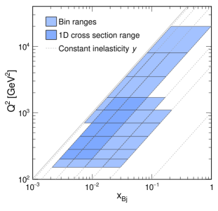
Figure 1: DIS kinematic plane as a function of $x_{\text{Bj}}$ and $Q^{2}$. The kinematic range of the measurement is displayed as colored area. The dark shaded area indicates the kinematic range of the reported single-differential cross section ($200\leq Q^{2}<1700\,\mathrm{GeV}^{2}$ and $0.2\leq y<0.7$).

The kinematic range is limited by acceptance, resolution, and trigger: The polar-angle acceptance of the LAr calorimeter, $\theta\lesssim 154^{\circ}$, defines the $Q^{2}$ region of the measurement, $Q^{2}>150\,\mathrm{GeV}^{2}$; The electron energy acceptance corresponds to $y\lesssim 0.7$ for $Q^{2}\lesssim 1000\,\mathrm{GeV}^{2}$; The inelasticity is required to be $y>0.05$, since acceptance and resolution deteriorate for lower $y$, where the hadronic angle $\gamma_{h}$ becomes small and the Lorentz-factor $\beta$ of the boost vector approaches unity.

The binning used in this analysis is also presented in Table 1.

Observable	Binning name	Notation	Binning
$\tau_{1}^{b}$	$\tau_{1}^{b}$ nominal	$b_{\tau_{1}^{b}}^{(11)}$	$[0,0.05,0.1,0.15,0.22,0.3,0.4,0.54,0.72,0.86,0.98,1.0+\epsilon]$
$\tau_{1}^{b}$	$\tau_{1}^{b}$ coarse	$b_{\tau_{1}^{b}}^{(8)}$	$[0,0.05,0.1,0.15,0.22,0.3,0.4,0.6,1.0+\epsilon]$
$\tau_{1}^{b}$	$\tau_{1}^{b}$ coarse low $y$	$b_{\tau_{1}^{b}}^{(7)}$	$[0,0.1,0.15,0.22,0.3,0.4,0.6,1.0+\epsilon]$
$y$	$y$	$b_{y}$	$[0.05,0.1,0.2,0.4,0.7,0.94]$
$Q^{2}$	$Q^{2}$	$b_{Q^{2}}$	$[150,200,280,440,700,1100,1700,3500,8000,20000[$ $\mathrm{GeV}^{2}$

Table 1: Binnings used in the analysis.

Over most of the phase space the binning is dictated by the resolution of $\tau_{1}^{b}$. Coarser binning is chosen at the boundaries of the kinematic range due to the following factors:

• low $y$ or large $Q^{2}$: large values of $\tau_{1}^{b}$ have low statistics or lower resolution;

• low $y$ and $\tau_{1}^{b}<0.05$: very low cross section which cannot be resolved.

Altogether 308 cross section values are measured. The respective highest $\tau_{1}^{b}$ bins ($0.98\leq\tau_{1}^{b}\leq 1$ and $0.6<\tau_{1}^{b}\leq 1$) include events with $\tau_{1}^{b}=1$, in which the current hemisphere is empty. Such events are related to low values of $x$ [46, 51, 61], and are present because $\tau_{1}^{b}$ is defined in the Breit frame. They are absent for event shape observables defined in the partonic center-of-mass frame, like thrust in $e^{+}e^{-}$ collisions [43, 61].

3 Monte Carlo simulations and model predictions

MC event generators are used to correct the data for detector acceptance and resolution effects, and for contributions from $ep$ collisions outside the phase-space of this analysis. The generated events are processed with a detailed simulation of the H1 detector based on GEANT3 [84], supplemented by fast shower simulations [85, 86, 87, 88, 89, 90]. The simulated data are reconstructed and processed with the same analysis algorithm as the real data [91, 92, 93, 94, 95, 96, 97].

Detector effects are corrected using regularized unfolding, based on the simulation of NC DIS events using the MC event generators Djangoh 1.4 [98] and Rapgap 3.1 [99]. Djangoh uses Born level matrix elements for NC DIS and dijet production and applies the color dipole model from Ariadne [100] for higher-order emissions. Rapgap implements Born level matrix elements for NC DIS and dijet production and uses the leading logarithmic approximation for parton shower emission. Both generators are interfaced to Heracles [101] for higher order QED effects at the lepton vertex. Both generators utilise the CTEQ6L parton distribution function (PDF) set [102] and the Lund hadronization model [103, 104]. Hadronization model parameters were determined by the ALEPH Collaboration [105].

Contributions to the event yield from processes other than NC DIS are simulated with a variety of MC event generators. Photoproduction events are simulated using Pythia 6.2 [106, 107]. Events with di-lepton production are generated using Grape [108]. A sample of QED Compton events is simulated using the program Compton [109]. Deeply virtual Compton scattering (DVCS) is simulated with Milou [110]. NC DIS events for lower values of $Q^{2}$ and for charged current DIS are simulated with Djangoh. Overall, more than $3.4\times 10^{8}$ signal events were simulated with Djangoh and Rapgap, and about $5.3\times 10^{8}$ events were simulated in total.

The fully-corrected $\tau_{1}^{b}$ cross section measurements are compared to a set of theoretical predictions. The following classes of prediction are studied: two common MC event generators as used at HERA; three modern general-purpose event generators which are widely used in high-energy physics; one dedicated event generator incorporating transverse-momentum dependent effects; and two variants of fixed-order predictions. In order to explore the sensitivity of the data to various QCD effects, in each MC event generator one element is varied, such as the parton shower model, the fixed-order prediction and its matching or merging procedure with the parton shower, the hadronization model, or the PDF set. The fixed-order predictions include variations of the renormalization and factorization scales. In addition, dedicated predictions for the inclusive NC DIS cross sections are studied. The following MC event generators from the HERA era are considered:

• Djangoh 1.4 and Rapgap 3.1, similar to those described above, but with radiative effects switched off in Heracles.

The following modern MC event generators are studied:

• Pythia 8.3 [111, 112], where the impact of the parton-shower is studied by employing three different parton-shower models: i) ‘default’ dipole-like $p_{\perp}$-ordered shower with a local dipole recoil strategy (Pythia 8.310) [113], ii) $p_{\perp}$-ordered Vincia parton shower based on the antenna formalism at leading color (Pythia 8.307) [114, 115, 116, 117], and iii) the Dire [118, 119, 120] parton shower which is an improved dipole-shower with additional treatment of collinear enhancements (Pythia 8.307). All models use the Pythia 8.3 default Lund string model for hadronization [112] and the PDF4LHC21 PDF set [121] for the hard PDFs. The Vincia and Dire parton shower use a value of 0.118 for the strong coupling at the mass of the $Z$ boson.

• Powheg Box plus Pythia (Powheg+Pythia) [122] implements predictions in NLO QCD matched to parton showers using the Powheg method [123, 124], where the radiation phase space is parameterised according to the Frixione-Kunszt-Signer (FKS) subtraction technique [125]. Dedicated momentum mappings preserve the DIS kinematic variables. The NLO predictions (up to $\mathcal{O}(\alpha_{\rm s})$) are then interfaced to parton showers and hadronziation from Pythia 8.308.

• Herwig 7.2 [126], where the impact of different modelling of the hard interaction and its merging or matching with the parton-shower model is studied in three variants: The default prediction implements leading-order matrix elements supplemented with an angular-ordered parton shower [127] and cluster hadronization model [128, 129]. The second variant utilises MC@NLO [130] which implements NLO matrix element corrections. Matching with the default angular-ordered parton shower is performed [131]. The third variant also utilises NLO matrix elements, but with dipole merging and a dipole parton shower [131]. Herwig-generated events are further processed with Rivet [132].

• Sherpa 2.2 [133, 134], where the modelling of hadronization effects can be studied by using two different hadronization models. The default Sherpa 2.2 predictions are based on multi-leg tree-level matrix elements from Comix [135] that are combined in the CKKW merging formalism [136] with dipole showers [137, 138] and supplemented with the cluster hadronization as implemented in AHADIC++ [139]. As an alternative prediction, the parton-level calculation is supplemented with the Lund string fragmentation model [140].

• Predictions from the pre-release version of Sherpa 3.0 [141] are provided by the Sherpa authors featuring a new cluster hadronization model [142] and matrix element calculation at NLO QCD obtained from OpenLoops [143] with the Sherpa dipole shower [138] based on the truncated shower method [144, 145]. The predictions are associated with scale uncertainties from a 7-point scale variation by factors of two.

The following dedicated MC event generators are studied:

• Cascade 3 [146] implements off-shell processes via the automated matrix element calculators KaTie [147] and Pegasus [148], parton shower and hadronization through Pythia 6. This utilises transverse momentum dependent (TMD) PDF sets in the parton branching (PB) methodology [149]. Two PB TMD PDF sets are studied, denoted as set 1 and set 2 [150]. They differ primarily in the scale choice for QCD evolution.

The following exact QCD predictions are studied:

• Next-to-next-to-leading order (NNLO) predictions in perturbative QCD up to third order in $\alpha_{\rm s}$ ($\mathcal{O}(\alpha_{\rm s}^{3})$) are obtained for the process $ep\to e+2\text{jets}+X$ with the program NNLOJET [151, 152, 153, 55]. The factorization and renormalization scales are chosen to be $\mu=Q$. Scale uncertainties are determined by the largest difference in the 7-point scale-variation prescription, with scale factors 0.5 and 2. The PDF set PDF4LHC21 [121] is used. Non-perturbative correction factors are applied to these parton-level predictions as multiplicative correction factors for hadronization effects. These NNLO predictions are valid only in the region where the $ep\to e+2\text{jets}+X$ process dominates and hadronization corrections are small. This corresponds to the region $\tau_{1}^{b}\gtrsim 0.1$ and $\tau_{1}^{b}\neq 1$. The NNLO predictions can formally be brought to next-to-next-to-next-to-leading (N3LO) order for NC DIS using the projection to Born method [154, 55].

• Analytic predictions are provided in NNLO$\otimes$NLL${}^{\prime}\otimes$Had accuracy [155], using NLO pQCD matrix elements for dijet production projected onto the NNLO NC DIS cross section [156] and supplemented with automatised next-to-leading logarithmic accuracy using the Caesar framework [58, 56, 57] as implemented in the Sherpa framework [157]. For these predictions, hadronization corrections are applied as a multiplicative correction matrix obtained from Sherpa 3.0 [158].

Further predictions for $\tau_{1}^{b}$ have been reported previously but are not available here. These include NNLO predictions supplemented with parton shower [156], next-to-next-to-leading logarithmic and next-to-NLL predictions [159], analytic NLL predictions [61], and N3LO predictions using the projection to Born method and a dispersive model for hadronization effects [154, 55].

The following predictions are compared to the inclusive NC DIS cross sections measured in bins of $Q^{2}$ and $y$:

• Predictions in NNLO pQCD are obtained with the program Apfel++ [160, 161], using the three loop splitting and coefficient functions [162, 163, 164, 165] together with the PDF set NNPDF31_nnlo_as_0118. The predictions are associated with PDF uncertainties and with scale uncertainties, where the latter are defined as 7-point scale variations in the coefficient functions. An alternative prediction is obtained with the H1PDF2017NNLO PDF set [166].

• Predictions in approximate next-to-next-to-next-to-leading order (aN3LO) are obtained for inclusive NC DIS cross sections using the program Apfel++ [160, 161] and using the MSHT PDFs at a3NLO order [167] and four-loup splitting functions from Refs. [168, 169, 170].

4 Data correction: regularized unfolding

The data are corrected for detector effects, background processes, and higher-order QED effects using regularized unfolding [171, 172]. This section presents the unfolding procedure and the measurement of the fully-corrected cross section. In addition, correction factors for hadronization and electroweak effects are discussed.

The signal Monte Carlo generators Djangoh and Rapgap are used together with the detailed simulation of the H1 detector to generate synthetic detector-level events along with corresponding particle-level events (MC event simulation). Within the scope of the analysis, the detector response is found to be well modelled in all studied aspects, which is essential for obtaining accurate unfolding results. Figure 2 shows comparison of these simulations to data for the observables $Q^{2}$, $y$, and $\tau_{1}^{b}$.

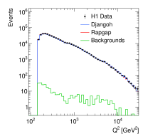
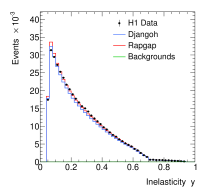
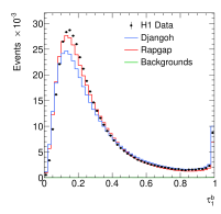
Figure 2: Detector level distributions of $Q^{2}$ (left), $y$ (middle), and $\tau_{1}^{b}$ (right) of the selected data. The definition of these observables is given by Eq. (5) and (6). The data are compared to the MC event simulations Djangoh and Rapgap. Both simulations include estimated background contributions from processes other than high-$Q^{2}$ NC DIS, as indicated by the green line (visible on logarithmic scale).

Both MC event simulations, although based on different physics models, are found to describe the data well. Comparisons to other observables, related closely to the detector performance, are discussed in the following.

Figure 3 shows the distribution of $P_{z}^{\text{Breit}}$, the particle-candidate longitudinal momentum in the Breit frame, compared with simulations for reconstructed clusters and tracks. Good overall agreement between simulations and data is observed, for both clusters and tracks.

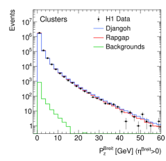
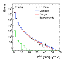
Figure 3: The longitudinal momentum $P_{z}^{\text{Breit}}$ in the Breit frame of reconstructed particle candidates in the selected events. Only particle candidates with $\eta^{\text{Breit}}>0$ are displayed, since only those contribute to the actual calculation of $\tau_{1}^{b}$. Particle candidates are defined by an energy-flow algorithm taking clusters and tracks into account. Left: the $P_{z}^{\text{Breit}}$ distribution for clusters not associated with a track, right: the $P_{z}^{\text{Breit}}$ distribution for objects associated with a track. The detector-level data are compared to the MC event simulations Djangoh and Rapgap, which include further MC samples for background processes. Further details are given in the Figure 2 caption.

The measurement of $\tau_{1}^{b}$  includes only particle candidates of the current hemisphere. Figure 4 shows relative contributions from different polar angular regions $\theta$ and particle energies $E$. The largest contributions are from objects in the central detector ($25<\theta<153^{\circ}$), and from objects with large energy ($E>1.0\,\mathrm{GeV}$). Both types of object are measured well by the relevant H1 sub-detector components, and are modelled well by the MC event simulations.

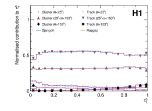
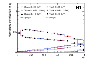
Figure 4: Left: The normalized contribution to $\tau_{1}^{b}$ for differently reconstructed particle candidates (tracks or clusters as defined in Figure 3) in three distinct polar regions $\theta$. The regions are chosen according to $\theta$-ranges, where different components of the H1 detector are relevant for particle reconstruction [69, 70, 71, 72]. Right: The normalised contribution to $\tau_{1}^{b}$ for different ranges of particle energies $E$ and for differently reconstructed particle candidates. The data are compared to the MC event simulations Djangoh and Rapgap. The relative contributions are obtained by calculating a weight $w=\sum_{\text{contrib}}P_{z}^{\text{Breit}}/\sum_{\text{all}}P_{z}^{\text{Breit}}$ for each event and each contribution. The resulting distributions are normalized to the $\tau_{1}^{b}$ distribution.

At the particle level (also denoted as generator or hadron level), the scattered electron is identified with the electron emitted at the DIS vertex. In the case of a photon radiated off the incoming or scattered lepton, the photon is recombined with the scattered electron if the angular distance is smaller than the angular distance to the $-z$-axis; otherwise it is removed from the event record.

The HFS is formed from all remaining particles with proper lifetime $c\tau>10\,\text{mm}$. The DIS kinematic observables at the particle level are then computed using equations (5) and (6).

The triple-differential cross section is reported as a function of $\tau_{1}^{b}$ in bins of $(Q^{2},y)$, and is obtained as

$$\frac{d\sigma_{i}}{d\tau_{1}^{b}}(Q^{2},y)=\frac{\left(A^{+}(\vec{n}_{\text{data}}-\vec{n}_{\text{Bkg}})\right)_{i}}{\mathcal{L}\cdot\Delta_{\tau_{1}^{b},i}}\cdot c_{\text{QED},i}\,,$$ (7)

where $\vec{n}_{\text{data}}$ denotes a large data vector of event counts; $\vec{n}_{\text{Bkg}}$ is a corresponding vector with the estimated number of events from processes other than high-$Q^{2}$ inclusive NC DIS; $\Delta_{\tau_{1}^{b},i}$ is the bin width of the $i$th bin of the respective $\tau_{1}^{b}$ distribution; and $A^{+}$ denotes the regularized inverse of the detector response matrix. The parameter $c_{\text{QED}}$ is the QED correction factor, and $\mathcal{L}$ specifies the integrated luminosity of the measurement. For this analysis, $\mathcal{L}=351.1\,\text{pb}^{-1}$ [66], where the $e^{+}$ beam data contribute an integrated luminosity of 191.0 pb^-1, and the $e^{-}$ beam data have an integrated luminosity of 160.1 pb^-1.

The detector response matrix $A$ is determined using both signal MC event simulators. The TUnfold package [172] is used to calculate the regularised inverse $A^{+}$ and to propagate its uncertainties. Finer binning is used at detector than at particle level; typically there are 12 bins in the detector-level histogram. The vector $\vec{n}$ has 4331 entries in the extended detector-level phase space, $0.01<y<0.94$ and $Q^{2}>60\,\mathrm{GeV}^{2}$, and the vector $A^{+}\vec{n}$ has 572 entries at the particle level. The extended detector-level phase space in $y$ and $Q^{2}$ accounts for migrations into and out of the fiducial measurement phase space. In order to obtain the final 324 cross section points from the 572 values, two adjacent values are combined each, with exceptions made at lowest and largest $\tau_{1}^{b}$. This procedure stabilizes the unfolding and reduces dependencies on the MC models. The regularization procedure employs the so-called curvature mode of TUnfold, which approximates second derivatives, and it acts on the differences of the unfolded results and the MC predictions as a bias distribution. The regularization is applied separately for each $\tau_{1}^{b}$ distribution in the individual ($Q^{2},y$) intervals. The regularization parameter is set to a small value $\tau=10^{-3.2}$ as suggested by the analysis of Stein’s Unbiased Risk Estimator, SURE [173]. The regularization has a moderate impact on the result, and reduces large fluctuations and sizable negative correlations between adjacent data points in some regions of the analysis.

The background vector $\vec{n}_{\text{Bkg}}$ consists of events from photoproduction, charged current DIS, di-lepton production, and DVCS processes. A small number of simulated events which are outside the enlarged phase space at particle level (e.g. $y<0.01$, or $Q^{2}<120\,\mathrm{GeV}^{2}$) but migrate into the enlarged detector-level phase space are treated as background, and are also included in $\vec{n}_{\text{Bkg}}$ (“acceptance correction”).

The multiplicative factor $c_{\text{QED}}$ corrects the data for higher-order QED effects and for the positron charge. It is defined as the ratio of the cross section predicted without ($\sigma_{\text{norad}}^{e^{-}p}$) to the one with QED radiative effects ($\sigma_{\text{rad}}$). The factors are determined using the Djangoh event generator, where higher-order QED effects are implemented from Heracles [101]. The factors are validated with Rapgap. The denominator $\sigma_{\text{rad}}$ includes radiative cross sections for electron–proton and positron–proton scattering with relative integrated luminosity weights as for real data. The numerator $\sigma_{\text{norad}}^{e^{-}p}$ is defined for non-radiative electron–proton scattering ($e^{-}p$). The resulting cross section measurements are therefore reported for $e^{-}p$ scattering.  The effects of longitudinal polarization of the lepton beam are negligible, due to a nearly balanced mixture of running periods with opposite lepton beam helicities. The QED correction $c_{\text{QED}}$ corrects for first-order real emission of photons off the lepton line, including QED Compton enhancement, photonic vertex correction, and purely photonic self-energy contributions at the external lepton lines. This defines the non-radiative cross section level ($\sigma_{\text{norad}}^{e^{-}p}$), which is reported as the main result of the paper. The data still include higher-order purely weak effects, self-energy corrections of the exchanged bosons, second order electroweak corrections, and photon-PDF induced contributions.

The QED correction factors $c_{\text{QED}}$ are largely independent of the kinematic variables $\tau_{1}^{b}$, $Q^{2}$, and $y$ owing to the use of the I$\Sigma$ method and the treatment of radiated photons at the radiative particle level. Effectively, $c_{\text{QED}}$ corrects mainly for the cut on the longitudinal energy-momentum balance ($(E-P_{z})_{\text{gen}}>45\,\mathrm{GeV}$), which has no effect at the non-radiative cross section level, but is active at the radiative particle-level. When the inverse of $c_{\text{QED}}$ is applied, the cross section at the radiative level discussed above is obtained (see also Ref. [83]), where the treatment of radiated photons is relevant.

To enable comparison with a range of theoretical calculations, additional correction factor are determined which optionally can be applied:

• The correction factor $c_{\text{NoZ}}$ corrects further for all leading and subleading electroweak corrections, which are $\gamma Z$ and pure $Z$-exchange, and first order purely weak vertex, self-energy and box corrections. Hence, only leptonic and hadronic corrections to the photon self-energy remain ($\sigma_{\gamma-\text{only}}$).

• The correction factor $c_{\text{Born}}$ corrects further to the so-called DIS Born level ($\sigma_{\text{Born}}^{e^{-}p}$), where first order purely weak vertex, self-energy and box corrections are corrected. In addition, corrections for leptonic and hadronic contributions to the photon and $Z$ self-energy are applied.

• The correction factor $c_{e^{+}p}$ corrects the reported $e^{-}p$ non-radiative cross sections to an $e^{+}p$ initial state ($\sigma_{\text{norad}}^{e^{+}p}$).

The QED correction factor and the optional correction factors can be summarized as:

$$\begin{array}[]{cc}c_{\text{QED}}=\frac{\sigma_{\text{norad}}^{e^{-}p}}{\sigma_{\text{rad}}}\,,&c_{\text{NoZ}}=\frac{\sigma_{\gamma-\text{only}}}{\sigma_{\text{norad}}^{e^{-}p}}\,,\\ c_{\text{Born}}=\frac{\sigma_{\text{Born}}^{e^{-}p}}{\sigma_{\text{norad}}^{e^{-}p}}\,,&c_{e^{+}p}=\frac{\sigma_{\text{norad}}^{e^{+}p}}{\sigma_{\text{norad}}^{e^{-}p}}\,.\end{array}$$ (8)

The single-differential cross section as a function of $\tau_{1}^{b}$  in the NC DIS kinematic range, $200<Q^{2}<1700\,\mathrm{GeV}^{2}$ and $0.2<y<0.7$, is obtained by integrating the triple differential cross section for $\tau_{1}^{b}$ over $(Q^{2},y)$. The inclusive NC DIS cross section as a function of $Q^{2}$ and $y$ is obtained by integrating the $\tau_{1}^{b}$ distribution over the $(Q^{2},y)$ range. The single-differential and the inclusive NC DIS cross sections, $\tfrac{d\sigma}{d\tau_{1}^{b}}$ and $\tfrac{d^{2}\sigma}{dQ^{2}dy}$, are reported separately for $e^{-}p$ and $e^{+}p$ scattering, where only data from the respective running periods were analyzed. Unfolding is carried out separately for $e^{+}p$ and $e^{-}p$ data in these cases.

The result of integrating the $\tau_{1}^{b}$ distribution, as described above, is consistent with the inclusive DIS cross section reported previously [74]. However, the present measurement is not corrected to the bin center but is reported in intervals of $Q^{2}$ and $y$, whereas previous inclusive DIS cross section measurements were reported as a function of $Q^{2}$ and $x_{\text{Bj}}$ [174, 175, 176, 79, 177, 74]. This is the first inclusive NC DIS cross section measurement at HERA that is corrected using regularised unfolding.

Fixed order calculations do not account for non-perturbative effects due to hadronization of partons into stable hadrons. Such effects can approximately be accounted for by means of bin-wise multiplicative correction factors $c_{\text{Had}}$, defined as the ratio of calculated particle-level and parton-level cross sections. Such hadronization corrections are determined using Djangoh and Rapgap, which are found to be consistent with each other. These factors are also validated using Pythia 8.3. The hadronization correction factors approximately decrease like $1/Q$, and are found to be similar in size to hadronization corrections reported for $e^{+}e^{-}$ at $\sqrt{s}\sim Q$ at PETRA [178, 179, 20].

5 Uncertainties

The measurement is affected by a number of systematic effects. The following sources of uncertainties are considered:

• Statistical uncertainties of the data are propagated to the unfolded cross sections. This procedure results in bin-to-bin correlations, which are provided as supplementary material on the H1 webpage [180].

• The energy of the scattered lepton is measured with a precision of 0.5 % in the central and backward region of the detector, and with $1\,\%$ precision in the forward region of the detector [74]. The efficiency of the electron identification algorithm is studied with an alternative track-based algorithm and the data and MC simulation are found to agree within 0.2 % at lower $Q^{2}$ and 1 % for $Q^{2}>3500\,\mathrm{GeV}^{2}$  [181, 74].

• The energies of all clusters and tracks receive scale factors from a dedicated jet energy calibration [78, 73]. This calibration procedure results in two independent uncertainty contributions, whether clusters are contained in jets or not. The two contributions are denoted as ‘jet energy scale uncertainty’ (JES) and ‘remaining cluster energy scale uncertainty’ (RCES), and both uncertainties are determined by varying the energy of the respective HFS objects by $\pm 1\,\%$. As compared to the JES, the RCES typically affects objects with lower transverse momenta.

• The polar-angle position of the LAr calorimeter with respect to the Central Tracking Detector (CTD) is aligned with a precision of 1 mrad [74]. This uncertainty component is considered separately for the scattered electron and for the HFS objects.

• The unfolding procedure is associated with several uncertainties. Differences in the migration matrix $A$ when determined from Djangoh or Rapgap are denoted as ‘model’ uncertainty. Half of the difference in each element $A_{ij}$ is propagated to the unfolded cross section. This applies also to events that migrate from outside the particle-level phase space into detector-level phase space, and to events that are generated in the particle-level phase space but are not reconstructed at detector-level. Statistical uncertainties in $A$ from the limited event sample of the simulations are also considered. The size of the regularization parameter has an uncertainty of 50 % and that variation is propagated to the resulting cross sections [172]. The considered variation covers alternative procedures to determine the regularization strength, including the minimum global correlation coefficient or the $L$-curve scan [172].

• Other uncertainty components are found to be negligible on their own, and a conservative bin-to-bin uncorrelated uncertainty of 0.5 % is introduced to cover the sum of these. An example of the uncertainties included here is the vertex and electron track reconstruction efficiency, which has an uncorrelated uncertainty of 0.2 % [181], The distance between the calorimeter cluster of the scattered electron and a vertex-associated track is not described perfectly by the simulation, and the corresponding efficiency correction introduces an uncorrelated uncertainty of about 0.1 to 0.2 %. The uncertainty associated with the choice of the regularization strength in the unfolding procedure is found to be below 0.1 %. The contributions from other processes than high-$Q^{2}$ NC DIS (backgrounds) are estimated from MC simulations and a normalization uncertainty of 100 % is considered, which results in an uncertainty smaller than 0.1 %.

• The normalization uncertainty is found to be 2.7 %, and is dominated by the uncertainty on the integrated luminosity [66]. Other normalization uncertainties are negligible in comparison. For example, the efficiency of the trigger is found to be higher than 99.5 % [73, 74] and the related uncertainty is smaller than $0.5\%$. Further normalization uncertainties are related to the electron identification, the noise suppression algorithm in the LAr, and to the track and vertex identification.

• The QED correction factors were determined separately with Djangoh and Rapgap and very good agreement was found. While both MC generators implement QED corrections from Heracles, previous studies showed that these are consistent with the program Hector [182] and EPRC [183], and that the contribution from the two-photon exchange, which is not implemented in Heracles, is negligible [74, 184]. Consequently, the uncertainty of the QED correction factors represent only their statistical component, while other uncertainties would be of negligible size, when compared to other uncertainty sources.

• Uncertainties of the hadronization correction factors, relevant for a subset of the comparisons only, are determined as half of the difference between the correction factor obtained from Djangoh and Rapgap.

6 Results

Results for the single-differential and triple-differential 1-jettiness cross sections as well as for the double-differential inclusive NC DIS cross section are presented.

Single-differential cross sections as a function of $\tau_{1}^{b}$

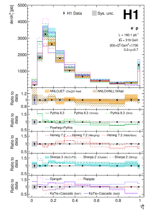
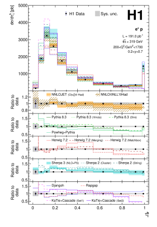
Figure 5: The differential cross section $d\sigma/d\tau_{1}^{b}$ in the kinematic region $200\leq Q^{2}/\,\mathrm{GeV}^{2}<1700$ and $0.2\leq y<0.7$ for $e^{+}p$ (left) and $e^{-}p$ scattering at $\sqrt{s}=319\,\mathrm{GeV}$. The data are corrected for detector effects (acceptance, resolution) and QED radiative effects. The statistical uncertainties are displayed as vertical error bars, systematic uncertainties as shaded areas. The data are compared to the MC predictions from NNLOJET, NNLO$\otimes$NLL${}^{\prime}\otimes$Had, Pythia 8.3, Powheg Box, Herwig 7.2, Sherpa 2.2, Sherpa 3.0, Djangoh, Rapgap, and KaTie+Cascade 3. Selected parameters are varied in the predictions as indicated in brackets. Colored areas indicate theoretical uncertainties associated with some of the predictions (see text). The lower panel displays the ratio of predictions to data.

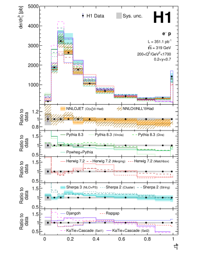
Figure 6: The differential cross section $d\sigma/d\tau_{1}^{b}$ in the kinematic region $200\leq Q^{2}/\,\mathrm{GeV}^{2}<1700$ and $0.2\leq y<0.7$ for $e^{-}p$ scattering at $\sqrt{s}=319\,\mathrm{GeV}$. The data are recorded with electron and positron beams, and corrected to $e^{-}p$ cross sections using Heracles. Further details are given in the caption of Figure 5.

The single-differential 1-jettiness cross sections $\tfrac{d\sigma}{d\tau_{1}^{b}}$ in NC DIS $ep$ scattering in the kinematic range $200\leq Q^{2}<1700$ $\mathrm{GeV}^{2}$ and $0.2\leq y<0.7$ are measured for $e^{+}p$ and $e^{-}p$ collisions in Tables 2 and 3 and displayed in Figure 5. As no significant differences are observed between the two cross sections, the measurement is repeated using the sum of both datasets, corrected to $e^{-}p$ scattering cross sections, in Table 4 and Figure 6. The statistical uncertainty in the data is typically around 2 to 4 % and the systematic uncertainty is of order 4 %. Larger uncertainties are seen for the lowest $\tau_{1}^{b}$ bin. The differential $\tau_{1}^{b}$ cross section exhibits a distinct peak at $\tau_{1}^{b}\sim 0.13$ and a tail towards high values of $\tau_{1}^{b}$. The distinct DIS peak is populated by DIS Born-level kinematics with a single hard parton, the position and shape of which are dominated by hadronization and resummation effects. The tail region is populated by events with hard radiation, including two-jet topologies in the far tail. The cross section at $\tau_{1}^{b}\simeq 1$ has a sizeable value, as it includes events with empty current hemisphere in the Breit frame. This event configuration can occur at low $x_{\text{Bj}}$ and is studied in a dedicated publication [185]. The data are compared to predictions from NNLOJET up to $\mathcal{O}(\alpha_{\rm s}^{3})$ in the strong coupling; resummed predictions at NLL accuracy matched to fixed-order predictions at $\mathcal{O}(\alpha_{\rm s}^{2})$ and corrected for hadronization; various predictions from the modern MC event generators Pythia 8.3, Sherpa 2.2, Sherpa 3.0, Herwig 7.2, and Powheg Box plus Pythia; as well as to the dedicated MC event generators for DIS, Djangoh, Rapgap, and KaTie+Cascade. The agreement between the predictions and data are very similar for $e^{+}p$ and $e^{-}p$ cross sections. Further details are discussed below.

Triple-differential cross sections as a function of $\tau_{1}^{b}$, $Q^{2}$, and $y$

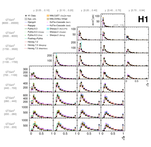
Figure 7: The triple-differential cross section $\tfrac{d^{3}\sigma}{d\tau_{1}^{b}dQ^{2}dy}$, presented as $\tfrac{d\sigma}{d\tau_{1}^{b}}$ in regions of $Q^{2}$ and $y$. The $Q^{2}$ and $y$ ranges are displayed on the left and top, respectively. Each panel displays the differential cross section $d\sigma/d\tau_{1}^{b}$ in that phase space. The data are displayed as full circles, the vertical error bars indicate statistical uncertainties, while systematic uncertainties are displayed as shaded area. The data are compared to predictions from NNLOJET, NNLO$\otimes$NLL${}^{\prime}\otimes$Had, Pythia 8.3, Powheg Box, Herwig 7.2, Sherpa 2.2, Sherpa 3.0, Djangoh, Rapgap, and KaTie+Cascade 3. Selected parameters are varied in the predictions as indicated. The ratios of the data and predictions to the Sherpa 3.0 predictions are displayed in Figures 8–12. At highest $Q^{2}$ ($8000<Q^{2}/\mathrm{GeV}^{2}<20\,000\,$) only a single $y$ interval is measured, $0.2<y<0.94$.

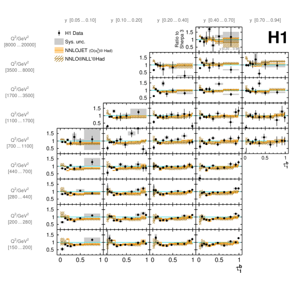
Figure 8: The ratio of data and NNLOJET ($\mathcal{O}(\alpha_{s}^{3})$) and NNLO$\otimes$NLL${}^{\prime}\otimes$Had predictions to the Sherpa 3.0 predictions for the triple-differential cross section $\tfrac{d^{3}\sigma}{d\tau_{1}^{b}dQ^{2}dy}$. See Figure 7 caption for further details. The data are displayed as full circles, the vertical error bars indicate statistical uncertainties, while systematic uncertainties are displayed as shaded area. The shaded coloured area indicates the theoretical uncertainty associated with the NNLOJET predictions. The hatched area indicates the theoretical uncertainty associated with the NNLO$\otimes$NLL${}^{\prime}\otimes$Had predictions.

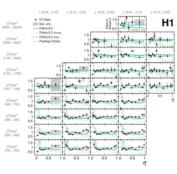
Figure 9: The ratio of data and Pythia 8.3 predictions to the Sherpa 3.0 predictions for the triple-differential cross section $\tfrac{d^{3}\sigma}{d\tau_{1}^{b}dQ^{2}dy}$. See Figure 7 caption for further details. The data are displayed as full circles, the vertical error bars indicate statistical uncertainties, while systematic uncertainties are displayed as shaded area. The full dark green line indicates predictions from Pythia 8.3 employing the default parton shower adapted for DIS kinematics, the short dashed line indices predictions using the Vincia parton shower, and the long dashed line the Dire parton shower. The green full line shows predictions from Powheg Box interfaced to parton shower and hadronization from Pythia 8.3.

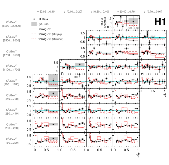
Figure 10: The ratio of data and Herwig 7.2 predictions to the Sherpa 3.0 predictions for the triple-differential cross section $\tfrac{d^{3}\sigma}{d\tau_{1}^{b}dQ^{2}dy}$. See Figure 7 caption for further details. The data are displayed as full circles, the vertical error bars indicate statistical uncertainties, while systematic uncertainties are displayed as shaded area. The full line indicates predictions from Sherpa 3.0, and the shaded coloured are associated theoretical uncertainties. The short and long dashed lines indicate predictions from Sherpa 2.2, where two hadronisation models are studies, Cluster and String hadronisation model, respectively.

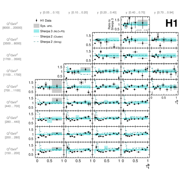
Figure 11: The ratio of data and Sherpa 2 predictions to Sherpa 3.0 predictions for the triple-differential cross section $\tfrac{d^{3}\sigma}{d\tau_{1}^{b}dQ^{2}dy}$. See Figure 7 caption for further details. The data are displayed as full circles, the vertical error bars indicate statistical uncertainties, while systematic uncertainties are displayed as shaded area. The full dark green line indicates predictions from Pythia 8.3 employing the default parton shower adapted for DIS kinematics, the short dashed line indices predictions using the Vincia parton shower, and the long dashed line the Dire parton shower. The green full line shows predictions from Powheg Box interfaced to parton shower and hadronization from Pythia 8.3.

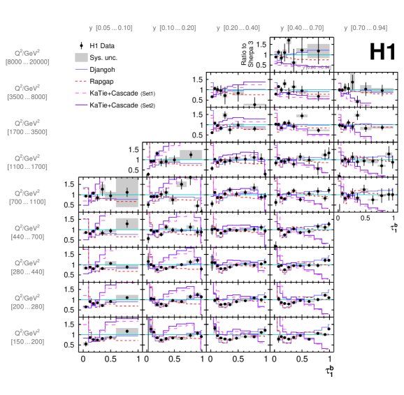
Figure 12: The ratio of data and predictions from dedicated DIS MC event generators to the Sherpa 3.0 predictions for the triple-differential cross section $\tfrac{d^{3}\sigma}{d\tau_{1}^{b}dQ^{2}dy}$ for adjacent regions in $Q^{2}$ and $y$. See Figure 7 caption for further details. The data are displayed as full circles, the vertical error bars indicate statistical uncertainties, while systematic uncertainties are displayed as shaded area. The full blue line indicates predictions from Djangoh, the red dashed line from Rapgap, and the pink dashed and violet line line show predictions from KaTie+Cascade 3 for two different TMD PDFs and scale choices.

Triple-differential cross sections are presented in Tables 5– 36 and are displayed in Figure 7. The ratio of the data and predictions to the predictions from Sherpa 3.0 are displayed in Figures 8–12. The triple differential cross sections are presented in the kinematic range $150<Q^{2}<20\,000\,\mathrm{GeV}^{2}$ and $0.05<y<0.94$ as a function of $\tau_{1}^{b}$. Regions that are kinematically forbidden or experimentally inaccessible are omitted. At highest $Q^{2}$ only a single combined $y$ region ($0.2<y<0.94$) is presented due to low event counts.

Events with a harder virtuality $Q$ produce more collimated particles, effectively shifting the DIS peak position in the $\tau_{1}^{b}$ distributions towards lower values. In addition, a reduced phase space for hard radiation at high $Q^{2}$ tends to lower the differential cross section in the larger $\tau_{1}^{b}$ region relative to the peak region. The relative contribution of topologies with $\tau_{1}^{b}$ close to unity increases with $y$ for fixed $Q$. Equivalently, that contribution increases as $x_{Bj}$ decreases.

Comparison to exact QCD predictions

The fixed order predictions with NLL resummation of large logarithms (NNLO$\otimes$NLL${}^{\prime}\otimes$Had) provide an accurate description of the entire $\tau_{1}^{b}$ distribution within their uncertainties. These predictions include resummation and are matched to the NNLO inclusive DIS cross section ($\alpha_{\rm s}^{2}$), such that they are valid over the entire $\tau_{1}^{b}$ range. Formally, they are one order lower in $\alpha_{s}$ than the NNLOJET predictions.

The NNLO dijet predictions from NNLOJET ($\alpha_{\rm s}^{3}$) provide a good description of the data within their uncertainty over their entire range of validity ($0.22<\tau_{1}^{b}<0.98$). Sizable hadronization corrections of up to $+40\,\%$ hinder quantitative comparisons and an interpretation in terms of underlying parameters of the theory; this point will have to be investigated in the future.

Comparison to modern MC event generators

The recent MC event generators Pythia 8.3, Powheg+Pythia, Herwig 7.2, Sherpa 2.2 and Sherpa 3.0 employ LO, multi-leg or NLO matrix elements matched to parton shower and hadronization models. Those generators generally provide a good description of the data.

The MC predictions from Pythia provide an overall reasonable description of the data, with small but visible differences between the three parton shower models studied. The default Pythia and Pythia+Vincia predictions overestimate the data at low $\tau_{1}^{b}<0.1$, whereas Pythia+Dire provides a good description. All three Pythia predictions are similar in the parton-shower region ($0.1<\tau_{1}^{b}<0.4$), but tend to underestimate the data in the tail region ($\tau_{1}^{b}>0.5$). The latter could be related to the fact that matrix elements for $eg\to eq\bar{q}$ enter at $\mathcal{O}(\alpha_{\rm s})$ only, and are not recovered properly in a parton shower emerging from $eq\to eq$ alone. The default Pythia predictions are a leading-order MC model and they benefit from a large value of $\alpha_{\rm s}(m_{\rm Z})$ for the parton shower, which is default in Pythia, and thus raises the prediction at larger $\tau_{1}^{b}$ and brings them closer to the data. Looking only at the single-differential cross sections, Pythia+Dire tends to overshoot the data in the parton-shower region, but from the triple-differential data it is evident that the discrepancy arises from events at lower values of $Q^{2}$. At very large values of $y$ ($y>0.7$), the Pythia+Dire predictions fail to describe the data at large values of $\tau_{1}^{b}$. The Pythia+Vincia prediction provides a good description of the data in the range $0.1\lesssim\tau_{1}^{b}\lesssim 0.5$. It has difficulties at larger values of $\tau_{1}^{b}$, presumably related to the fact that Vincia was developed for a symmetric collider setup and is not yet fully validated for the asymmetric beams of $ep$ collisions.

The predictions from Powheg Box are lower than the default Pythia predictions at medium to large $\tau_{1}^{b}$, and overshoot the data at low $\tau_{1}^{b}$. Larger values of $\alpha_{\rm s}(m_{\rm Z})$ in the simulation, or corrections beyond NLO DIS, such as NLO dijet matrix elements, may be required to improve the description of the data.

The Herwig variants are able to provide a good description of the data. Although the default predictions from Herwig 7.2 provide the worst description among all modern MC generators, a significant improvement is obtained with NLO matrix elements. The merging technique provides the best description among the Herwig predictions, with benefits particularly at larger $\tau_{1}^{b}$. All Herwig predictions fail to describe the lowest $\tau_{1}^{b}$ cross section ($\tau_{1}^{b}<0.05$). The default Herwig predictions exhibit a prominent structure at medium $\tau_{1}^{b}$.

The Sherpa 2.2 predictions provide a good description of the data, in particular at larger $\tau_{1}^{b}$. The two different hadronization models (String vs. Cluster) provide very similar predictions, which do not differ by more than the data uncertainties, albeit the string model is a bit closer to the data at medium $\tau_{1}^{b}$. Both Sherpa 2.2 predictions overshoot the data at lowest $\tau_{1}^{b}$ ($\tau_{1}^{b}<0.1$), and undershoot the data at $\tau_{1}^{b}\simeq 1$. The underprediction at high $\tau_{1}^{b}$ and overprediction at low $\tau_{1}^{b}$ seems to be a common feature of NLO+PS models, c.f. Powheg Box and Herwig.

The Sherpa 3.0 predictions with NLO matrix elements, improved parton shower and cluster hadronization model provide a better description of the data than those from Sherpa 2.2, and the predictions provide an accurate description of the data within the uncertainties. Only at lower $Q^{2}$ and values of $\tau_{1}^{b}\sim 0.3$ the Sherpa 3.0 predictions overestimate the data. A noteworthy improvement over other MC predictions is observed in the lowest $\tau_{1}^{b}$ region, where also good agreement with data is observed. This could be related to the modelling of an intrisic $k_{t}$ in Sherpa 3.0.

Comparison to MC event generators from the HERA era and dedicated DIS models

The DIS MC event generators Djangoh and Rapgap provide an overall satisfactory description of the data, although both have difficulties to describe the shape in the region $\tau_{1}^{b}<0.3$ accurately and both models underestimate the data in the range $0.1<\tau_{1}^{b}<0.3$. The high $\tau_{1}^{b}$ region is well described. Djangoh is somewhat higher than Rapgap in that region, which is consistent with the observation of a harder $P_{\text{T}}$-spectrum of jets [186]. The triple-differential cross sections are well described by Djangoh and Rapgap. At low $y$, Rapgap underestimates the high $\tau_{1}^{b}$ region more than Djangoh. Both models fail to describe the region $\tau_{1}^{b}<0.05$.

The KaTie+Cascade 3 predictions, employing TMD-sensitive PDF sets with two different choices for the QCD evolution scale, provide a reasonable description of the data. TMD PDF Set 2 provides one of the best descriptions at the low $\tau_{1}^{b}$ region, whereas the predictions with TMD PDF Set 1 are a bit higher. However, at lowest $Q^{2}$ and large $y$, also predictions from Set 2 overshoot the data significantly. In the region of larger $\tau_{1}^{b}$, the KaTie+Cascade 3 predictions fail to describe the data, likely related to the absence of $eg\to eq\bar{(}q)$ processes in the hard matrix elements.

Double-differential cross sections for inclusive neutral-current DIS as a function of $Q^{2}$ and $y$

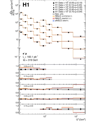
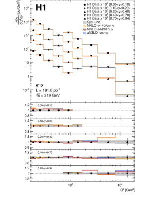
Figure 13: The double-differential inclusive neutral current DIS cross section $\tfrac{d^{2}\sigma_{\text{NC DIS}}}{dQ^{2}dy}$ for $e^{-}p$ (left) and $e^{+}p$ (right) scattering in the kinematic region $150\leq Q^{2}<20\,000\,\mathrm{GeV}^{2}$ and $0.05\leq y<0.94$. The data are displayed as full circles, the vertical error bars indicate statistical uncertainties, while systematic uncertainties are displayed as shaded area. Different $y$ ranges are indicated by different markers, and are displaced vertically by a constant factor as indicated in the legend. The vertical error bars indicate statistical uncertainties, whereas systematic experimental uncertainties are displayed as shaded area. The data are compared to NNLO and a3NLO predictions. The orange line indicates NNLO predictions using the H1PDF2017NNLO PDF set, the red line NNLO predictions using the NNPDF 3.1 PDF set, and the blue line indicates predictions in aN3LO accuracy using the MSHT PDF set. The hatched area indicates associated theoretical uncertainties from scale variations and PDF uncertainties.

The inclusive NC DIS cross sections $\tfrac{d^{2}\sigma_{\text{NC DIS}}}{dQ^{2}dy}$ are presented in Tables 37 and 38 and are displayed in Figure 13, where NNLO and aN3LO predictions for inclusive DIS are compared with the data. For comparisons with the NC DIS predictions, the data are corrected to the DIS Born level by applying the factor $c_{\text{B}orn}$. These cross sections are measured for $e^{+}p$ and $e^{-}p$ scattering by analyzing the data from the two lepton charges separately, including dedicated unfolding matrices and QED correction factors. The inclusive NC DIS cross sections $\tfrac{d^{2}\sigma_{\text{NC DIS}}}{dQ^{2}dy}$ are obtained by integrating over $\tau_{1}^{b}$ in every $(Q^{2},y)$ range. Hence, kinematic migrations due to limited resolution of the detector are corrected with high accuracy, since different configurations of the hadronic final state, represented by $\tau_{1}^{b}$, are considered in the unfolding. The inclusive NC DIS cross sections can be compared with predictions from structure function calculations, and serve as an important validation of the absolute size of the $\tau_{1}^{b}$ cross sections. These data constitute the first bin integrated inclusive NC DIS cross section measurements at HERA in $Q^{2}$ and $y$, employing proper regularized unfolding of detector effects. The results can be compared with predictions based on structure functions and serve as a crosscheck in the determination of the absolute normalization of the triple-differential cross section measurements. The NC DIS measurements are also used together with the triple-differential cross sections to obtain normalized 1-jettiness event shape distributions [180].

Predictions for inclusive NC DIS cross sections

The double-differential inclusive DIS $\tfrac{d^{2}\sigma_{\text{NC DIS}}}{dQ^{2}dy}$ are compared to predictions in NNLO and a3NLO accuracy. It is observed that both the NNLO and the a3NLO predictions provide a very good description of the $e^{+}p$ and $e^{-}p$ data in the entire kinematic range, and small discrepancies are observed only at lowest values of $y$ or largest values of $Q^{2}$. One can note that the H1 data [74, 187] are already included in the PDF determination, which is the basis of the predictions. Differences between the H1PDF2017NNLO PDF set and the NNPDF3.1 PDF set are small.

7 Summary

The first measurement of the 1-jettiness event shape observable in neutral-current deep-inelastic electron–proton scattering is presented. The measured 1-jettiness observable $\tau_{1}^{b}$ is equivalent to the classical event shape observable Thrust normalized with $\frac{Q}{2}$, $\tau_{zQ}$. It quantities the degree to which the hadronic final state in the current hemisphere is collimated along the exchanged bosons four-vector.

The data were recorded with the H1 experiment at the HERA collider operating with a center-of-mass energy of $\sqrt{s}=319\,\mathrm{GeV}$. A single-differential cross section is measured as a function of $\tau_{1}^{b}$ in the kinematic region $200\leq Q^{2}<1700\,\mathrm{GeV}^{2}$ and $0.2\leq y<0.7$. A triple-differential cross section as a function of $\tau_{1}^{b}$, $Q^{2}$, and $y$ is reported in the kinematic range $0\leq\tau_{1}^{b}\leq 1$, $150\leq Q^{2}<20\,000\,\mathrm{GeV}^{2}$, and $0.05\leq y<0.94$. The data are unfolded to the particle level and corrected for higher-order QED radiative effects.

Given typical accuracies of $4$–$20\,\%$ (single differential) and $6$–$30\,\%$ (triple-differentials), the data exhibit high sensitivity to the modelling of the hard interaction, to the parton shower and hadronization models in MC event generators. The unfolded data are compared to a variety of predictions. Most of the models studied provide a satisfactory description of the data. The classical MC event generators Djangoh and Rapgap, which were optimised for HERA physics, provide an overall good description. The more modern general purpose MC event generators Herwig 7.2, Pythia 8.3, Sherpa 2.2 and Sherpa 3.0 provide a good description of the data, although some problems remain to be resolved in regions of the phase-space specific for each model. When studying different parton shower or hadronization models, the potential of these data for the optimization of event generators is demonstrated.

Fixed order pQCD predictions provide a good description of the data, but sizeable non-perturbative corrections for hadronization effects have to be applied. When incorporating NLL resummation, such predictions are seen to be in good agreement with the data over the full range of $\tau_{1}^{b}$. Future pQCD analyses may be able to constrain parton distribution functions of the proton (PDFs) or the strong coupling constant from the data.

The $\tau_{1}^{b}$-integrated triple-differential cross sections are found to be in agreement with the previously measured double-differential inclusive NC DIS cross section. This provides an important consistency test of the data, but also a consistency check with the HERA legacy measurements of inclusive NC DIS. The inclusive NC DIS cross section is described by structure function calculations which are available up to aN3LO and which are free of hadronization effects. The 1-jettiness measurement as a function of $\tau_{1}^{b}$, $Q^{2}$, and $y$ can be viewed as a generalised NC DIS cross section, and is the first triple-differential measurement of this kind.

In summary, it is believed that these data will be highly valuable to improve MC event generators, which are of importance to achieve the physics goals of the HL-LHC physics program [188, 189]. Further improvements can be achieved when complemented with recent jet substructure measurements [190]. With an improved understanding of soft and non-perturbative effects, these data will become useful for the determination of PDFs or the value of the strong coupling constant $\alpha_{\rm s}(m_{\rm Z})$. The presented measurement at HERA can be complemented in the future with measurements in electron–proton collisions at lower center-of-mass energies at the electron–ion collider in Brookhaven (EIC) [191] or at higher energies at the LHeC or FCC-eh at CERN [192, 193, 191], or with measurements in $pp$ at the LHC.

1D 1-jettiness cross sections in $e^{-}p$ for $200<Q^{2}<1700\,\mathrm{GeV}^{2}$ and $0.2<y<0.7$ – $\text{d}\sigma/\text{d}\tau_{1}^{b}~{}[\rm pb/\Delta\tau_{1}^{b}]$ $\tau_{1}^{b}$ range Results Uncertainties Correction factors ${}_{\text{min}}$ ${}_{\text{max}}$ $\frac{\text{d}\sigma}{\text{d}\tau_{1}^{b}}$ ${}_{\text{stat}}$ ${}_{\text{RCES}}$ ${}_{\text{JES}}$ ${}_{\text{HadTh}}$ ${}_{\text{ElEn}}$ ${}_{\text{ElTh}}$ ${}_{\text{Model}}$ ${}_{\text{MCstat}}$ ${}_{\text{Unfold}}$ ${}_{\text{ElecID}}$ ${}_{\text{Lumi}}$ ${}_{\text{Uncor}}$ ${}_{\text{QED}}$ $c_{\text{QED}}$ $c_{\text{NoZ}}$ $c_{\text{Born}}$ $c_{\text{e+p}}$ $c_{\text{Had}}$ $\delta_{\text{HAD}}$ ${}_{[\text{pb}]}$ _{[%] [%] [%] [%] [%] [%] [%] [%] [%] [%] [%] [%] [%] [%]} 0.00 0.05 144.8 12.1 $-0.1$ $+1.6$ $+0.8$ $-0.6$ $+0.2$ $-15.6$ $0.5$ $-1.1$ 0.2 2.7 0.5 0.3 1.080 0.975 0.912 0.960 0.102 1.1 0.05 0.10 1827 2.4 $+0.5$ $+1.0$ $+0.3$ $-0.9$ $+0.3$ $-0.3$ $0.5$ $+0.1$ 0.2 2.7 0.5 0.1 1.070 0.981 0.909 0.974 0.769 1.3 0.10 0.15 3245 2.0 $-0.1$ $+0.6$ $+0.1$ $-0.4$ $+0.5$ $+4.0$ $0.6$ $+0.4$ 0.2 2.7 0.5 0.1 1.066 0.988 0.912 0.984 1.342 6.7 0.15 0.22 2635 2.2 $+0.2$ $+0.1$ $-0.1$ $-1.0$ $+0.6$ $+2.8$ $0.6$ $-0.6$ 0.2 2.7 0.5 0.1 1.065 0.989 0.913 0.990 1.397 1.1 0.22 0.30 1774 3.0 $+0.4$ $-0.3$ $-0.2$ $-0.7$ $+0.3$ $+2.5$ $0.6$ $-0.3$ 0.2 2.7 0.5 0.1 1.071 0.988 0.911 0.989 1.307 1.7 0.30 0.40 1028 3.9 $+0.8$ $-0.7$ $-0.2$ $-1.0$ $+0.4$ $+2.1$ $0.4$ $+0.5$ 0.2 2.7 0.5 0.1 1.071 0.987 0.912 0.989 1.311 4.5 0.40 0.54 675.7 3.4 $+1.0$ $-0.9$ $-0.2$ $-1.4$ $+0.5$ $+0.7$ $0.3$ $+0.1$ 0.2 2.7 0.5 0.1 1.069 0.989 0.912 0.991 1.303 6.5 0.54 0.72 417.5 3.4 $+0.5$ $-0.9$ $-0.2$ $-1.3$ $+0.5$ $-1.6$ $0.2$ $+0.0$ 0.2 2.7 0.5 0.1 1.076 0.987 0.909 0.991 1.268 5.1 0.72 0.86 290.1 4.7 $+0.0$ $-0.7$ $-0.1$ $-1.0$ $+0.5$ $-1.2$ $0.3$ $+0.1$ 0.2 2.7 0.5 0.2 1.075 0.989 0.911 0.992 1.243 2.1 0.86 0.98 285.6 4.5 $+0.0$ $-0.9$ $+0.1$ $-0.5$ $+0.5$ $-0.4$ $0.3$ $+0.0$ 0.2 2.7 0.5 0.2 1.073 0.992 0.913 0.994 1.340 1.6 0.98 1.00 1392 3.2 $-1.5$ $-0.2$ $-0.2$ $+0.0$ $+0.3$ $-1.0$ $0.2$ $-0.0$ 0.2 2.7 0.5 0.2 1.076 0.988 0.913 0.991 0.763 1.1

Table 2: Single differential 1-jettiness cross sections for $e^{-}p$ scattering in the range $200<Q^{2}<1700\,\mathrm{GeV}^{2}$ and $0.2<y<0.7$, $\text{d}\sigma/\text{d}\tau_{1}^{b}~{}[\rm pb/\Delta\tau_{1}^{b}]$. The $\tau_{1}^{b}$ ranges and the corresponding cross section measurements are indicated, together with the data statistical uncertainty (stat), and the systematic uncertainties: the hadronic (RCES and JES) and electron (ElEn) energy scale uncertainties, the hadron (HadTh) and electron (ElTh) polar angle uncertainties, the model uncertainty (Model), the simulation statistical uncertainty (MCstat), the unfolding uncertainty (Unfold), the electron identification uncertainty (ElecID), the luminosity uncertainty (Lumi), the residual uncorrelated uncertainty (Uncor), and the QED correction uncertainty (QED). The radiative correction factors are also shown.

1D 1-jettiness cross sections in $e^{+}p$ for $200<Q^{2}<1700\,\mathrm{GeV}^{2}$ and $0.2<y<0.7$ – $\text{d}\sigma/\text{d}\tau_{1}^{b}~{}[\rm pb/\Delta\tau_{1}^{b}]$ $\tau_{1}^{b}$ range Results Uncertainties Correction factors ${}_{\text{min}}$ ${}_{\text{max}}$ $\frac{\text{d}\sigma}{\text{d}\tau_{1}^{b}}$ ${}_{\text{stat}}$ ${}_{\text{RCES}}$ ${}_{\text{JES}}$ ${}_{\text{HadTh}}$ ${}_{\text{ElEn}}$ ${}_{\text{ElTh}}$ ${}_{\text{Model}}$ ${}_{\text{MCstat}}$ ${}_{\text{Unfold}}$ ${}_{\text{ElecID}}$ ${}_{\text{Lumi}}$ ${}_{\text{Uncor}}$ ${}_{\text{QED}}$ $c_{\text{QED}}$ $c_{\text{NoZ}}$ $c_{\text{Born}}$ $c_{\text{e+p}}$ $c_{\text{Had}}$ $\delta_{\text{HAD}}$ ${}_{[\text{pb}]}$ _{[%] [%] [%] [%] [%] [%] [%] [%] [%] [%] [%] [%] [%] [%]} 0.00 0.05 137.5 11.4 $+0.2$ $+1.7$ $+0.9$ $-0.8$ $+0.2$ $-15.2$ $0.5$ $-0.7$ 0.2 2.7 0.5 0.3 1.077 1.013 0.916 1.000 0.100 1.1 0.05 0.10 1841 2.1 $+0.8$ $+1.1$ $+0.4$ $-0.7$ $+0.5$ $+0.4$ $0.4$ $+0.7$ 0.2 2.7 0.5 0.1 1.070 1.005 0.916 1.000 0.761 1.1 0.10 0.15 3174 1.8 $+0.2$ $+0.5$ $-0.1$ $-0.6$ $+0.3$ $+4.1$ $0.6$ $-1.0$ 0.2 2.7 0.5 0.1 1.065 1.001 0.918 1.000 1.336 6.7 0.15 0.22 2580 1.9 $+0.0$ $-0.1$ $-0.1$ $-0.5$ $+0.4$ $+2.5$ $0.6$ $+0.7$ 0.2 2.7 0.5 0.1 1.067 0.997 0.917 1.000 1.400 1.1 0.22 0.30 1730 2.7 $+0.4$ $-0.2$ $-0.1$ $-1.1$ $+0.6$ $+2.5$ $0.5$ $+0.4$ 0.2 2.7 0.5 0.1 1.065 0.996 0.921 1.000 1.308 1.9 0.30 0.40 1099 3.3 $+0.8$ $-0.7$ $-0.2$ $-1.2$ $+0.4$ $+2.1$ $0.4$ $-1.5$ 0.2 2.7 0.5 0.1 1.067 0.995 0.920 1.000 1.311 4.3 0.40 0.54 651.7 3.2 $+1.1$ $-0.9$ $-0.2$ $-1.5$ $+0.5$ $+0.5$ $0.3$ $+0.5$ 0.2 2.7 0.5 0.1 1.068 0.996 0.919 1.000 1.302 6.7 0.54 0.72 419.5 3.1 $+0.6$ $-0.8$ $-0.2$ $-1.2$ $+0.5$ $-1.7$ $0.2$ $+0.4$ 0.2 2.7 0.5 0.1 1.072 0.994 0.917 1.000 1.269 5.1 0.72 0.86 298.2 4.3 $-0.0$ $-0.8$ $-0.1$ $-1.0$ $+0.5$ $-1.8$ $0.3$ $+0.1$ 0.2 2.7 0.5 0.2 1.072 0.994 0.917 1.000 1.243 2.2 0.86 0.98 337.4 3.7 $+0.1$ $-0.9$ $-0.0$ $-0.5$ $+0.4$ $-0.9$ $0.3$ $-0.0$ 0.2 2.7 0.5 0.2 1.071 0.995 0.919 1.000 1.340 1.6 0.98 1.00 1428 2.9 $-1.4$ $-0.2$ $-0.1$ $+0.1$ $+0.4$ $-1.4$ $0.2$ $-0.0$ 0.2 2.7 0.5 0.2 1.075 0.995 0.922 1.000 0.762 1.1

Table 3: Single differential 1-jettiness cross sections for $e^{+}p$ scattering in the range $200<Q^{2}<1700\,\mathrm{GeV}^{2}$ and $0.2<y<0.7$, $\text{d}\sigma/\text{d}\tau_{1}^{b}~{}[\rm pb/\Delta\tau_{1}^{b}]$. Further details are given in the caption of Tab. 2.

1D 1-jettiness cross sections in $e^{-}p$ ($\mathcal{L}=351.1\,\rm pb^{-1}$) for $200<Q^{2}<1700\,\mathrm{GeV}^{2}$ and $0.2<y<0.7$ – $\text{d}\sigma/\text{d}\tau_{1}^{b}~{}[\rm pb/\Delta\tau_{1}^{b}]$ $\tau_{1}^{b}$ range Results Uncertainties Correction factors ${}_{\text{min}}$ ${}_{\text{max}}$ $\frac{\text{d}\sigma}{\text{d}\tau_{1}^{b}}$ ${}_{\text{stat}}$ ${}_{\text{RCES}}$ ${}_{\text{JES}}$ ${}_{\text{HadTh}}$ ${}_{\text{ElEn}}$ ${}_{\text{ElTh}}$ ${}_{\text{Model}}$ ${}_{\text{MCstat}}$ ${}_{\text{Unfold}}$ ${}_{\text{ElecID}}$ ${}_{\text{Lumi}}$ ${}_{\text{Uncor}}$ ${}_{\text{QED}}$ $c_{\text{QED}}$ $c_{\text{NoZ}}$ $c_{\text{Born}}$ $c_{\text{e+p}}$ $c_{\text{Had}}$ $\delta_{\text{HAD}}$ ${}_{[\text{pb}]}$ _{[%] [%] [%] [%] [%] [%] [%] [%] [%] [%] [%] [%] [%] [%]} 0.00 0.05 149.8 7.8 $+0.0$ $+1.7$ $+0.9$ $-0.6$ $+0.2$ $-15.4$ $0.4$ $-1.2$ 0.2 2.7 0.5 0.2 1.101 0.975 0.912 0.960 0.102 1.1 0.05 0.10 1885 1.5 $+0.7$ $+1.1$ $+0.3$ $-0.8$ $+0.4$ $+0.0$ $0.3$ $+0.7$ 0.2 2.7 0.5 0.1 1.084 0.981 0.909 0.974 0.769 1.3 0.10 0.15 3227 1.2 $+0.1$ $+0.5$ $-0.0$ $-0.6$ $+0.4$ $+4.0$ $0.4$ $-0.8$ 0.2 2.7 0.5 0.1 1.073 0.988 0.912 0.984 1.342 6.7 0.15 0.22 2632 1.2 $+0.1$ $-0.0$ $-0.1$ $-0.8$ $+0.4$ $+2.7$ $0.4$ $+0.5$ 0.2 2.7 0.5 0.1 1.070 0.989 0.913 0.990 1.397 1.1 0.22 0.30 1770 1.7 $+0.4$ $-0.2$ $-0.1$ $-0.9$ $+0.5$ $+2.5$ $0.3$ $-0.1$ 0.2 2.7 0.5 0.1 1.072 0.988 0.911 0.989 1.307 1.7 0.30 0.40 1070 2.3 $+0.8$ $-0.7$ $-0.2$ $-1.1$ $+0.5$ $+2.2$ $0.3$ $-0.6$ 0.2 2.7 0.5 0.1 1.073 0.987 0.912 0.989 1.311 4.5 0.40 0.54 681.3 2.2 $+1.1$ $-0.9$ $-0.2$ $-1.5$ $+0.6$ $+0.6$ $0.2$ $+0.3$ 0.2 2.7 0.5 0.1 1.072 0.989 0.912 0.991 1.303 6.5 0.54 0.72 423.8 2.3 $+0.5$ $-0.9$ $-0.2$ $-1.3$ $+0.5$ $-1.6$ $0.2$ $+0.2$ 0.2 2.7 0.5 0.1 1.077 0.987 0.909 0.991 1.268 5.1 0.72 0.86 302 3.1 $+0.0$ $-0.8$ $-0.2$ $-1.0$ $+0.5$ $-1.4$ $0.2$ $+0.1$ 0.2 2.7 0.5 0.1 1.076 0.989 0.911 0.992 1.243 2.1 0.86 0.98 336.7 2.7 $+0.1$ $-0.9$ $+0.0$ $-0.5$ $+0.5$ $-0.5$ $0.2$ $-0.0$ 0.2 2.7 0.5 0.1 1.074 0.992 0.913 0.994 1.340 1.6 0.98 1.00 1422 2.2 $-1.4$ $-0.2$ $-0.2$ $+0.1$ $+0.3$ $-1.1$ $0.1$ $-0.0$ 0.2 2.7 0.5 0.1 1.079 0.988 0.913 0.991 0.763 1.1

Table 4: Single differential 1-jettiness cross sections for $e^{-}p$ ($\mathcal{L}=351.1\,\rm pb^{-1}$) scattering in the range $200<Q^{2}<1700\,\mathrm{GeV}^{2}$ and $0.2<y<0.7$, $\text{d}\sigma/\text{d}\tau_{1}^{b}~{}[\rm pb/\Delta\tau_{1}^{b}]$. Further details are given in the caption of Tab. 2.

Cross sections in $e^{-}p$ ($\mathcal{L}=351.1\,\rm pb^{-1}$) for $150<Q^{2}<200$ $\mathrm{GeV}^{2}$ and $0.05<y<0.10$ – $\text{d}\sigma/\text{d}\tau_{1}^{b}~{}[\rm pb/\Delta\tau_{1}^{b}]$ $\tau_{1}^{b}$ range Results Uncertainties Correction factors ${}_{\text{min}}$ ${}_{\text{max}}$ $\frac{\text{d}\sigma}{\text{d}\tau_{1}^{b}}$ ${}_{\text{stat}}$ ${}_{\text{RCES}}$ ${}_{\text{JES}}$ ${}_{\text{HadTh}}$ ${}_{\text{ElEn}}$ ${}_{\text{ElTh}}$ ${}_{\text{Model}}$ ${}_{\text{MCstat}}$ ${}_{\text{Unfold}}$ ${}_{\text{ElecID}}$ ${}_{\text{Lumi}}$ ${}_{\text{Uncor}}$ ${}_{\text{QED}}$ $c_{\text{QED}}$ $c_{\text{NoZ}}$ $c_{\text{Born}}$ $c_{\text{e+p}}$ $c_{\text{Had}}$ $\delta_{\text{HAD}}$ ${}_{[\text{pb}]}$ _{[%] [%] [%] [%] [%] [%] [%] [%] [%] [%] [%] [%] [%] [%]} 0.00 0.10 22.81 22.8 $+2.7$ $+1.8$ $+2.2$ $+4.4$ $+0.8$ $-11.0$ $2.3$ $+1.5$ 0.2 2.7 0.5 0.8 1.063 1.010 0.918 0.992 0.144 1.6 0.10 0.15 345.4 4.0 $+2.7$ $+1.1$ $+1.1$ $+3.7$ $+0.9$ $-2.9$ $1.3$ $+0.4$ 0.2 2.7 0.5 0.5 1.072 0.996 0.925 1.001 1.068 4.5 0.15 0.22 528.3 2.5 $+1.6$ $+0.4$ $+0.2$ $+3.0$ $+0.9$ $+4.0$ $0.9$ $+0.7$ 0.2 2.7 0.5 0.4 1.065 1.001 0.922 1.002 2.035 31.9 0.22 0.30 416.3 3.7 $+1.4$ $+0.1$ $+0.4$ $+4.6$ $+1.9$ $+7.6$ $1.7$ $-3.1$ 0.2 2.7 0.5 0.4 1.068 0.997 0.919 0.995 1.847 12.4 0.30 0.40 256.7 6.0 $+4.0$ $+0.8$ $+1.2$ $+3.2$ $+2.1$ $+6.4$ $2.7$ $-1.1$ 0.2 2.7 0.5 0.4 1.066 0.998 0.924 1.001 1.517 3.0 0.40 0.60 141.8 7.2 $+2.8$ $-0.0$ $+0.6$ $+3.6$ $+1.1$ $-1.5$ $1.6$ $+1.0$ 0.2 2.7 0.5 0.3 1.065 1.003 0.925 1.004 1.456 6.1 0.60 1.00 92.52 7.5 $+1.0$ $+1.2$ $+1.7$ $+4.8$ $+1.1$ $-10.7$ $1.5$ $+1.2$ 0.2 2.7 0.5 0.2 1.073 0.992 0.920 0.997 1.224 1.9

Table 5: Differential 1-jettiness cross sections for $e^{-}p$ ($\mathcal{L}=351.1\,\rm pb^{-1}$) scattering in the range $150<Q^{2}<200$ $\mathrm{GeV}^{2}$ and $0.05<y<0.10$, $\text{d}\sigma/\text{d}\tau_{1}^{b}~{}[\rm pb/\Delta\tau_{1}^{b}]$. Further details are given in the caption of Tab. 2.

Cross sections in $e^{-}p$ ($\mathcal{L}=351.1\,\rm pb^{-1}$) for $150<Q^{2}<200$ $\mathrm{GeV}^{2}$ and $0.10<y<0.20$ – $\text{d}\sigma/\text{d}\tau_{1}^{b}~{}[\rm pb/\Delta\tau_{1}^{b}]$ $\tau_{1}^{b}$ range Results Uncertainties Correction factors ${}_{\text{min}}$ ${}_{\text{max}}$ $\frac{\text{d}\sigma}{\text{d}\tau_{1}^{b}}$ ${}_{\text{stat}}$ ${}_{\text{RCES}}$ ${}_{\text{JES}}$ ${}_{\text{HadTh}}$ ${}_{\text{ElEn}}$ ${}_{\text{ElTh}}$ ${}_{\text{Model}}$ ${}_{\text{MCstat}}$ ${}_{\text{Unfold}}$ ${}_{\text{ElecID}}$ ${}_{\text{Lumi}}$ ${}_{\text{Uncor}}$ ${}_{\text{QED}}$ $c_{\text{QED}}$ $c_{\text{NoZ}}$ $c_{\text{Born}}$ $c_{\text{e+p}}$ $c_{\text{Had}}$ $\delta_{\text{HAD}}$ ${}_{[\text{pb}]}$ _{[%] [%] [%] [%] [%] [%] [%] [%] [%] [%] [%] [%] [%] [%]} 0.00 0.05 3.299 153.8 $-3.4$ $+2.9$ $+1.9$ $+0.1$ $+0.9$ $-38.8$ $10.6$ $-2.5$ 0.2 2.7 0.5 2.3 1.107 1.010 0.967 0.990 0.019 0.2 0.05 0.10 102.2 14.1 $+1.6$ $+1.5$ $+1.4$ $+4.3$ $-1.1$ $-18.5$ $2.6$ $+1.1$ 0.2 2.7 0.5 0.7 1.079 0.994 0.904 0.985 0.248 5.2 0.10 0.15 454.1 4.6 $+2.4$ $+1.6$ $+0.7$ $+0.3$ $+1.0$ $+0.0$ $2.0$ $-0.8$ 0.2 2.7 0.5 0.4 1.077 0.986 0.914 1.000 0.869 3.0 0.15 0.22 636.8 2.9 $+0.9$ $+0.6$ $+0.3$ $+2.3$ $+0.2$ $+3.7$ $1.4$ $-0.1$ 0.2 2.7 0.5 0.3 1.072 0.995 0.921 0.997 1.665 22.6 0.22 0.30 491.1 4.2 $+1.6$ $-0.3$ $-0.2$ $+2.2$ $+1.5$ $+7.6$ $1.9$ $+1.0$ 0.2 2.7 0.5 0.3 1.075 0.991 0.918 0.990 1.621 7.6 0.30 0.40 318.8 5.9 $+2.3$ $+0.2$ $+0.0$ $+1.7$ $+0.3$ $+6.1$ $1.8$ $-1.9$ 0.2 2.7 0.5 0.3 1.069 0.996 0.919 1.001 1.420 1.0 0.40 0.54 191.9 6.9 $+2.0$ $+0.3$ $+0.2$ $+1.3$ $+1.4$ $+0.7$ $1.3$ $+0.0$ 0.2 2.7 0.5 0.3 1.069 0.996 0.923 1.001 1.420 6.7 0.54 0.72 114 7.8 $+1.4$ $+0.6$ $+0.3$ $+1.4$ $+1.0$ $-6.8$ $1.0$ $+1.2$ 0.2 2.7 0.5 0.3 1.074 0.999 0.915 0.998 1.396 6.3 0.72 0.86 90.26 10.3 $+0.5$ $+0.3$ $-0.1$ $+1.4$ $+1.4$ $-5.3$ $1.2$ $+0.6$ 0.2 2.7 0.5 0.3 1.079 0.993 0.917 0.997 1.355 2.9 0.86 0.98 98.86 9.2 $+0.3$ $-0.1$ $-0.1$ $+2.3$ $+1.0$ $-4.6$ $1.1$ $-0.1$ 0.2 2.7 0.5 0.3 1.069 1.000 0.929 1.003 1.451 2.7 0.98 1.00 295.5 9.2 $-1.0$ $-0.6$ $-0.4$ $+2.7$ $+0.4$ $-4.3$ $0.8$ $-0.0$ 0.2 2.7 0.5 0.3 1.075 0.997 0.921 0.998 0.679 1.7

Table 6: Differential 1-jettiness cross sections for $e^{-}p$ ($\mathcal{L}=351.1\,\rm pb^{-1}$) scattering in the range $150<Q^{2}<200$ $\mathrm{GeV}^{2}$ and $0.10<y<0.20$, $\text{d}\sigma/\text{d}\tau_{1}^{b}~{}[\rm pb/\Delta\tau_{1}^{b}]$. Further details are given in the caption of Tab. 2.

Cross sections in $e^{-}p$ ($\mathcal{L}=351.1\,\rm pb^{-1}$) for $150<Q^{2}<200$ $\mathrm{GeV}^{2}$ and $0.20<y<0.40$ – $\text{d}\sigma/\text{d}\tau_{1}^{b}~{}[\rm pb/\Delta\tau_{1}^{b}]$ $\tau_{1}^{b}$ range Results Uncertainties Correction factors ${}_{\text{min}}$ ${}_{\text{max}}$ $\frac{\text{d}\sigma}{\text{d}\tau_{1}^{b}}$ ${}_{\text{stat}}$ ${}_{\text{RCES}}$ ${}_{\text{JES}}$ ${}_{\text{HadTh}}$ ${}_{\text{ElEn}}$ ${}_{\text{ElTh}}$ ${}_{\text{Model}}$ ${}_{\text{MCstat}}$ ${}_{\text{Unfold}}$ ${}_{\text{ElecID}}$ ${}_{\text{Lumi}}$ ${}_{\text{Uncor}}$ ${}_{\text{QED}}$ $c_{\text{QED}}$ $c_{\text{NoZ}}$ $c_{\text{Born}}$ $c_{\text{e+p}}$ $c_{\text{Had}}$ $\delta_{\text{HAD}}$ ${}_{[\text{pb}]}$ _{[%] [%] [%] [%] [%] [%] [%] [%] [%] [%] [%] [%] [%] [%]} 0.00 0.05 7.584 48.1 $-0.6$ $+1.1$ $+1.0$ $+1.3$ $+0.6$ $-34.2$ $7.2$ $+6.3$ 0.2 2.7 0.5 1.9 1.047 1.015 0.954 0.979 0.018 0.2 0.05 0.10 101.9 10.4 $+1.3$ $+1.6$ $+0.2$ $-1.7$ $-0.2$ $-18.1$ $2.4$ $+0.5$ 0.2 2.7 0.5 0.6 1.085 0.994 0.911 0.980 0.209 3.4 0.10 0.15 376.1 4.5 $+1.3$ $+2.3$ $+1.0$ $+0.5$ $+0.7$ $+0.2$ $1.7$ $-0.5$ 0.2 2.7 0.5 0.3 1.067 1.002 0.926 0.998 0.714 1.6 0.15 0.22 647.2 2.5 $+1.1$ $+0.3$ $-0.1$ $+0.3$ $+0.3$ $+4.6$ $1.1$ $+0.2$ 0.2 2.7 0.5 0.2 1.072 0.996 0.920 0.998 1.402 13.4 0.22 0.30 581.7 3.0 $+0.8$ $-0.0$ $-0.4$ $-1.2$ $+0.8$ $+6.1$ $1.1$ $-0.3$ 0.2 2.7 0.5 0.2 1.081 0.991 0.914 0.995 1.447 1.1 0.30 0.40 337.6 4.7 $+1.0$ $+0.4$ $+0.2$ $-0.1$ $+0.8$ $+4.0$ $0.9$ $+0.2$ 0.2 2.7 0.5 0.2 1.073 1.000 0.917 0.990 1.341 0.8 0.40 0.54 214.6 4.8 $+1.3$ $+0.3$ $+0.0$ $-0.5$ $+0.8$ $+2.1$ $0.6$ $+0.3$ 0.2 2.7 0.5 0.2 1.065 0.997 0.920 1.003 1.379 6.4 0.54 0.72 148.1 4.7 $+0.9$ $-0.2$ $-0.2$ $-1.0$ $+0.7$ $-1.0$ $0.5$ $-0.3$ 0.2 2.7 0.5 0.2 1.074 0.995 0.917 0.995 1.375 7.4 0.72 0.86 103.6 6.6 $+0.2$ $-0.2$ $-0.0$ $-0.4$ $+0.8$ $-4.8$ $0.6$ $-0.1$ 0.2 2.7 0.5 0.2 1.073 0.997 0.916 0.999 1.349 4.0 0.86 0.98 133.4 5.1 $+0.2$ $-0.5$ $-0.0$ $+0.3$ $+0.7$ $-4.6$ $0.5$ $-0.0$ 0.2 2.7 0.5 0.2 1.079 0.992 0.918 0.994 1.461 3.2 0.98 1.00 576.5 3.8 $-1.1$ $-0.3$ $-0.2$ $+1.4$ $+0.5$ $-7.2$ $0.3$ $-0.0$ 0.2 2.7 0.5 0.2 1.079 0.996 0.915 0.995 0.707 1.8

Table 7: Differential 1-jettiness cross sections for $e^{-}p$ ($\mathcal{L}=351.1\,\rm pb^{-1}$) scattering in the range $150<Q^{2}<200$ $\mathrm{GeV}^{2}$ and $0.20<y<0.40$, $\text{d}\sigma/\text{d}\tau_{1}^{b}~{}[\rm pb/\Delta\tau_{1}^{b}]$. Further details are given in the caption of Tab. 2.

Cross sections in $e^{-}p$ ($\mathcal{L}=351.1\,\rm pb^{-1}$) for $150<Q^{2}<200$ $\mathrm{GeV}^{2}$ and $0.40<y<0.70$ – $\text{d}\sigma/\text{d}\tau_{1}^{b}~{}[\rm pb/\Delta\tau_{1}^{b}]$ $\tau_{1}^{b}$ range Results Uncertainties Correction factors ${}_{\text{min}}$ ${}_{\text{max}}$ $\frac{\text{d}\sigma}{\text{d}\tau_{1}^{b}}$ ${}_{\text{stat}}$ ${}_{\text{RCES}}$ ${}_{\text{JES}}$ ${}_{\text{HadTh}}$ ${}_{\text{ElEn}}$ ${}_{\text{ElTh}}$ ${}_{\text{Model}}$ ${}_{\text{MCstat}}$ ${}_{\text{Unfold}}$ ${}_{\text{ElecID}}$ ${}_{\text{Lumi}}$ ${}_{\text{Uncor}}$ ${}_{\text{QED}}$ $c_{\text{QED}}$ $c_{\text{NoZ}}$ $c_{\text{Born}}$ $c_{\text{e+p}}$ $c_{\text{Had}}$ $\delta_{\text{HAD}}$ ${}_{[\text{pb}]}$ _{[%] [%] [%] [%] [%] [%] [%] [%] [%] [%] [%] [%] [%] [%]} 0.00 0.05 19.92 23.3 $+0.4$ $+2.1$ $+1.9$ $+0.5$ $+0.8$ $-23.5$ $8.7$ $-7.8$ 0.2 2.7 0.5 1.8 1.111 0.970 0.850 0.933 0.017 0.2 0.05 0.10 45.17 21.7 $-2.7$ $-0.4$ $+0.3$ $+1.3$ $+0.5$ $-11.3$ $3.0$ $-1.6$ 0.2 2.7 0.5 0.5 1.054 1.012 0.918 1.006 0.180 2.1 0.10 0.15 265.3 6.0 $-0.1$ $+1.2$ $-0.3$ $+0.1$ $-0.2$ $+2.0$ $1.9$ $+2.4$ 0.2 2.7 0.5 0.3 1.066 0.992 0.914 0.994 0.630 1.4 0.15 0.22 509 3.1 $-0.6$ $+0.8$ $+0.4$ $-0.6$ $+0.7$ $+6.3$ $1.2$ $-1.6$ 0.2 2.7 0.5 0.2 1.074 0.991 0.917 0.991 1.252 9.0 0.22 0.30 457.6 3.7 $-1.5$ $-1.1$ $-0.3$ $-0.6$ $+0.5$ $+3.9$ $1.1$ $+1.3$ 0.2 2.7 0.5 0.2 1.074 0.994 0.918 0.995 1.357 2.4 0.30 0.40 302.5 5.1 $-0.9$ $-2.1$ $-0.4$ $-0.4$ $+0.3$ $+3.2$ $0.9$ $-1.9$ 0.2 2.7 0.5 0.2 1.077 0.991 0.919 0.996 1.302 2.5 0.40 0.54 195.5 5.5 $+0.3$ $-2.3$ $-0.3$ $-1.2$ $+0.4$ $+5.7$ $0.7$ $+0.5$ 0.2 2.7 0.5 0.2 1.079 0.989 0.916 0.990 1.363 5.9 0.54 0.72 103.4 6.9 $+0.3$ $-2.1$ $-0.2$ $-1.2$ $+0.6$ $+1.5$ $0.5$ $+0.8$ 0.2 2.7 0.5 0.2 1.073 0.997 0.922 0.997 1.368 7.8 0.72 0.86 101 7.4 $-0.6$ $-1.7$ $-0.2$ $-0.9$ $+0.5$ $+2.8$ $0.9$ $-0.2$ 0.2 2.7 0.5 0.2 1.077 0.993 0.918 0.997 1.343 4.8 0.86 0.98 103.1 6.4 $-0.8$ $-1.5$ $-0.0$ $-0.4$ $+0.5$ $-2.5$ $0.5$ $-0.1$ 0.2 2.7 0.5 0.2 1.078 0.996 0.917 0.993 1.471 3.4 0.98 1.00 566.2 4.2 $-1.9$ $-0.3$ $-0.1$ $+0.7$ $+0.2$ $-1.8$ $0.3$ $-0.0$ 0.2 2.7 0.5 0.2 1.079 0.993 0.917 0.993 0.727 1.7

Table 8: Differential 1-jettiness cross sections for $e^{-}p$ ($\mathcal{L}=351.1\,\rm pb^{-1}$) scattering in the range $150<Q^{2}<200$ $\mathrm{GeV}^{2}$ and $0.40<y<0.70$, $\text{d}\sigma/\text{d}\tau_{1}^{b}~{}[\rm pb/\Delta\tau_{1}^{b}]$. Further details are given in the caption of Tab. 2.

Cross sections in $e^{-}p$ ($\mathcal{L}=351.1\,\rm pb^{-1}$) for $200<Q^{2}<280$ $\mathrm{GeV}^{2}$ and $0.05<y<0.10$ – $\text{d}\sigma/\text{d}\tau_{1}^{b}~{}[\rm pb/\Delta\tau_{1}^{b}]$ $\tau_{1}^{b}$ range Results Uncertainties Correction factors ${}_{\text{min}}$ ${}_{\text{max}}$ $\frac{\text{d}\sigma}{\text{d}\tau_{1}^{b}}$ ${}_{\text{stat}}$ ${}_{\text{RCES}}$ ${}_{\text{JES}}$ ${}_{\text{HadTh}}$ ${}_{\text{ElEn}}$ ${}_{\text{ElTh}}$ ${}_{\text{Model}}$ ${}_{\text{MCstat}}$ ${}_{\text{Unfold}}$ ${}_{\text{ElecID}}$ ${}_{\text{Lumi}}$ ${}_{\text{Uncor}}$ ${}_{\text{QED}}$ $c_{\text{QED}}$ $c_{\text{NoZ}}$ $c_{\text{Born}}$ $c_{\text{e+p}}$ $c_{\text{Had}}$ $\delta_{\text{HAD}}$ ${}_{[\text{pb}]}$ _{[%] [%] [%] [%] [%] [%] [%] [%] [%] [%] [%] [%] [%] [%]} 0.00 0.10 45.03 8.0 $+1.8$ $+1.4$ $+1.1$ $-1.4$ $+0.5$ $-8.9$ $0.9$ $+2.3$ 0.2 2.7 0.5 0.6 1.062 0.993 0.929 0.997 0.220 2.2 0.10 0.15 445.6 2.1 $+2.2$ $+0.7$ $+0.6$ $-1.6$ $+0.6$ $-0.4$ $0.8$ $-0.6$ 0.2 2.7 0.5 0.4 1.083 0.989 0.907 0.992 1.767 24.8 0.15 0.22 495.6 1.7 $+0.6$ $+0.1$ $-0.2$ $-0.9$ $+0.5$ $+4.7$ $0.8$ $-0.8$ 0.2 2.7 0.5 0.4 1.068 0.991 0.909 0.998 2.198 28.3 0.22 0.30 328.5 3.0 $+0.2$ $+0.1$ $-0.6$ $-1.2$ $+0.4$ $+8.9$ $1.5$ $-2.1$ 0.2 2.7 0.5 0.4 1.067 0.991 0.913 1.003 1.617 1.6 0.30 0.40 147.8 6.5 $+4.0$ $-0.4$ $+0.3$ $-3.3$ $+1.2$ $+1.2$ $1.9$ $+6.8$ 0.2 2.7 0.5 0.4 1.064 0.998 0.911 0.998 1.447 2.5 0.40 0.60 96.42 4.9 $+2.8$ $+0.1$ $+0.7$ $-2.3$ $+1.5$ $-3.9$ $1.1$ $-3.0$ 0.2 2.7 0.5 0.4 1.078 0.987 0.903 0.987 1.407 5.6 0.60 1.00 53.08 6.2 $+0.8$ $+0.4$ $+0.7$ $-1.4$ $+0.3$ $-10.7$ $1.1$ $-1.0$ 0.2 2.7 0.5 0.3 1.079 0.994 0.913 0.990 1.189 1.2

Table 9: Differential 1-jettiness cross sections for $e^{-}p$ ($\mathcal{L}=351.1\,\rm pb^{-1}$) scattering in the range $200<Q^{2}<280$ $\mathrm{GeV}^{2}$ and $0.05<y<0.10$, $\text{d}\sigma/\text{d}\tau_{1}^{b}~{}[\rm pb/\Delta\tau_{1}^{b}]$. Further details are given in the caption of Tab. 2.

Cross sections in $e^{-}p$ ($\mathcal{L}=351.1\,\rm pb^{-1}$) for $200<Q^{2}<280$ $\mathrm{GeV}^{2}$ and $0.10<y<0.20$ – $\text{d}\sigma/\text{d}\tau_{1}^{b}~{}[\rm pb/\Delta\tau_{1}^{b}]$ $\tau_{1}^{b}$ range Results Uncertainties Correction factors ${}_{\text{min}}$ ${}_{\text{max}}$ $\frac{\text{d}\sigma}{\text{d}\tau_{1}^{b}}$ ${}_{\text{stat}}$ ${}_{\text{RCES}}$ ${}_{\text{JES}}$ ${}_{\text{HadTh}}$ ${}_{\text{ElEn}}$ ${}_{\text{ElTh}}$ ${}_{\text{Model}}$ ${}_{\text{MCstat}}$ ${}_{\text{Unfold}}$ ${}_{\text{ElecID}}$ ${}_{\text{Lumi}}$ ${}_{\text{Uncor}}$ ${}_{\text{QED}}$ $c_{\text{QED}}$ $c_{\text{NoZ}}$ $c_{\text{Born}}$ $c_{\text{e+p}}$ $c_{\text{Had}}$ $\delta_{\text{HAD}}$ ${}_{[\text{pb}]}$ _{[%] [%] [%] [%] [%] [%] [%] [%] [%] [%] [%] [%] [%] [%]} 0.00 0.05 11.36 35.5 $+0.2$ $+1.2$ $+1.8$ $-0.6$ $+0.9$ $-26.9$ $4.7$ $-2.2$ 0.2 2.7 0.5 1.6 1.097 0.961 0.918 0.999 0.031 0.4 0.05 0.10 137.6 8.2 $+1.3$ $+1.9$ $+1.0$ $-2.1$ $+0.7$ $-8.2$ $1.5$ $+1.1$ 0.2 2.7 0.5 0.5 1.089 0.996 0.910 1.000 0.402 7.2 0.10 0.15 513.3 3.3 $+1.7$ $+0.8$ $+0.6$ $-0.3$ $+0.6$ $-0.6$ $1.5$ $-1.7$ 0.2 2.7 0.5 0.3 1.077 0.988 0.908 0.995 1.398 18.7 0.15 0.22 518 2.9 $-0.5$ $-0.0$ $-0.5$ $-2.0$ $+0.2$ $+6.2$ $1.3$ $+1.8$ 0.2 2.7 0.5 0.3 1.067 0.992 0.915 0.990 1.848 20.7 0.22 0.30 369.6 4.3 $+0.6$ $+0.2$ $+0.1$ $-0.6$ $+0.9$ $+6.1$ $1.7$ $-2.5$ 0.2 2.7 0.5 0.3 1.073 0.994 0.915 0.990 1.476 1.2 0.30 0.40 185.9 7.5 $+2.0$ $-0.7$ $-0.5$ $-1.8$ $+1.1$ $+2.7$ $1.4$ $+4.0$ 0.2 2.7 0.5 0.3 1.073 0.991 0.919 0.989 1.389 2.7 0.40 0.54 148.9 5.8 $+2.0$ $-0.4$ $+0.1$ $-2.0$ $+1.2$ $-5.2$ $1.1$ $-1.5$ 0.2 2.7 0.5 0.3 1.074 0.989 0.912 0.992 1.385 7.5 0.54 0.72 82.71 6.6 $+1.0$ $-0.0$ $+0.1$ $-2.1$ $+1.0$ $-4.8$ $0.7$ $-1.3$ 0.2 2.7 0.5 0.3 1.069 1.002 0.919 0.999 1.335 5.1 0.72 0.86 68.07 8.3 $+0.2$ $-0.4$ $-0.3$ $-1.1$ $+0.6$ $-5.3$ $1.0$ $-0.4$ 0.2 2.7 0.5 0.3 1.071 0.995 0.920 0.998 1.297 2.0 0.86 0.98 72.56 8.2 $-0.7$ $-1.0$ $-0.4$ $+0.2$ $+0.8$ $-6.2$ $1.0$ $+0.0$ 0.2 2.7 0.5 0.3 1.071 1.003 0.920 0.993 1.383 1.9 0.98 1.00 230.1 7.4 $-1.8$ $-0.6$ $-0.6$ $-0.2$ $+0.6$ $-2.5$ $0.7$ $+0.2$ 0.2 2.7 0.5 0.4 1.069 0.998 0.919 1.007 0.696 1.6

Table 10: Differential 1-jettiness cross sections for $e^{-}p$ ($\mathcal{L}=351.1\,\rm pb^{-1}$) scattering in the range $200<Q^{2}<280$ $\mathrm{GeV}^{2}$ and $0.10<y<0.20$, $\text{d}\sigma/\text{d}\tau_{1}^{b}~{}[\rm pb/\Delta\tau_{1}^{b}]$. Further details are given in the caption of Tab. 2.

Cross sections in $e^{-}p$ ($\mathcal{L}=351.1\,\rm pb^{-1}$) for $200<Q^{2}<280$ $\mathrm{GeV}^{2}$ and $0.20<y<0.40$ – $\text{d}\sigma/\text{d}\tau_{1}^{b}~{}[\rm pb/\Delta\tau_{1}^{b}]$ $\tau_{1}^{b}$ range Results Uncertainties Correction factors ${}_{\text{min}}$ ${}_{\text{max}}$ $\frac{\text{d}\sigma}{\text{d}\tau_{1}^{b}}$ ${}_{\text{stat}}$ ${}_{\text{RCES}}$ ${}_{\text{JES}}$ ${}_{\text{HadTh}}$ ${}_{\text{ElEn}}$ ${}_{\text{ElTh}}$ ${}_{\text{Model}}$ ${}_{\text{MCstat}}$ ${}_{\text{Unfold}}$ ${}_{\text{ElecID}}$ ${}_{\text{Lumi}}$ ${}_{\text{Uncor}}$ ${}_{\text{QED}}$ $c_{\text{QED}}$ $c_{\text{NoZ}}$ $c_{\text{Born}}$ $c_{\text{e+p}}$ $c_{\text{Had}}$ $\delta_{\text{HAD}}$ ${}_{[\text{pb}]}$ _{[%] [%] [%] [%] [%] [%] [%] [%] [%] [%] [%] [%] [%] [%]} 0.00 0.05 16.71 23.2 $+0.3$ $+1.7$ $+1.8$ $-1.5$ $+0.3$ $-30.4$ $3.9$ $-9.2$ 0.2 2.7 0.5 1.3 1.044 1.002 0.940 1.023 0.027 0.3 0.05 0.10 122.6 8.4 $+1.2$ $+1.6$ $+1.0$ $-0.9$ $+0.3$ $-8.8$ $1.5$ $+2.4$ 0.2 2.7 0.5 0.4 1.068 0.997 0.917 0.992 0.332 4.7 0.10 0.15 507.5 3.1 $-0.0$ $+1.1$ $-0.1$ $-0.4$ $+0.3$ $+2.4$ $1.2$ $-2.3$ 0.2 2.7 0.5 0.3 1.070 0.996 0.921 0.992 1.145 12.5 0.15 0.22 543.5 2.7 $+0.8$ $+0.3$ $+0.2$ $-1.3$ $+1.1$ $+4.8$ $1.0$ $+2.1$ 0.2 2.7 0.5 0.2 1.067 0.998 0.921 1.000 1.563 10.5 0.22 0.30 418.1 3.5 $+0.5$ $+0.1$ $+0.0$ $-0.5$ $+0.7$ $+2.1$ $1.0$ $-2.2$ 0.2 2.7 0.5 0.2 1.071 0.993 0.917 0.994 1.347 4.6 0.30 0.40 226.8 5.6 $+0.9$ $-0.4$ $-0.2$ $-1.3$ $+0.5$ $+3.5$ $0.7$ $+1.5$ 0.2 2.7 0.5 0.2 1.074 0.991 0.916 0.992 1.343 3.1 0.40 0.54 162.3 4.9 $+1.4$ $-0.4$ $-0.2$ $-1.7$ $+0.6$ $+1.4$ $0.6$ $+0.1$ 0.2 2.7 0.5 0.2 1.072 0.992 0.913 0.991 1.357 7.0 0.54 0.72 106.6 5.0 $+0.9$ $-0.3$ $-0.2$ $-1.3$ $+0.7$ $-2.8$ $0.4$ $-0.4$ 0.2 2.7 0.5 0.2 1.078 0.990 0.912 0.992 1.321 5.9 0.72 0.86 82.38 6.5 $+0.2$ $-0.4$ $-0.2$ $-0.9$ $+0.7$ $-3.9$ $0.5$ $-0.6$ 0.2 2.7 0.5 0.2 1.076 0.994 0.914 0.998 1.291 2.8 0.86 0.98 79.12 6.6 $+0.2$ $-0.9$ $+0.0$ $-0.5$ $+0.5$ $-1.4$ $0.5$ $-0.2$ 0.2 2.7 0.5 0.2 1.074 0.996 0.915 0.996 1.390 2.1 0.98 1.00 353.2 4.8 $-1.1$ $-0.3$ $-0.2$ $-0.2$ $+0.5$ $-2.0$ $0.3$ $+0.0$ 0.2 2.7 0.5 0.3 1.081 0.991 0.919 0.992 0.729 1.5

Table 11: Differential 1-jettiness cross sections for $e^{-}p$ ($\mathcal{L}=351.1\,\rm pb^{-1}$) scattering in the range $200<Q^{2}<280$ $\mathrm{GeV}^{2}$ and $0.20<y<0.40$, $\text{d}\sigma/\text{d}\tau_{1}^{b}~{}[\rm pb/\Delta\tau_{1}^{b}]$. Further details are given in the caption of Tab. 2.

Cross sections in $e^{-}p$ ($\mathcal{L}=351.1\,\rm pb^{-1}$) for $200<Q^{2}<280$ $\mathrm{GeV}^{2}$ and $0.40<y<0.70$ – $\text{d}\sigma/\text{d}\tau_{1}^{b}~{}[\rm pb/\Delta\tau_{1}^{b}]$ $\tau_{1}^{b}$ range Results Uncertainties Correction factors ${}_{\text{min}}$ ${}_{\text{max}}$ $\frac{\text{d}\sigma}{\text{d}\tau_{1}^{b}}$ ${}_{\text{stat}}$ ${}_{\text{RCES}}$ ${}_{\text{JES}}$ ${}_{\text{HadTh}}$ ${}_{\text{ElEn}}$ ${}_{\text{ElTh}}$ ${}_{\text{Model}}$ ${}_{\text{MCstat}}$ ${}_{\text{Unfold}}$ ${}_{\text{ElecID}}$ ${}_{\text{Lumi}}$ ${}_{\text{Uncor}}$ ${}_{\text{QED}}$ $c_{\text{QED}}$ $c_{\text{NoZ}}$ $c_{\text{Born}}$ $c_{\text{e+p}}$ $c_{\text{Had}}$ $\delta_{\text{HAD}}$ ${}_{[\text{pb}]}$ _{[%] [%] [%] [%] [%] [%] [%] [%] [%] [%] [%] [%] [%] [%]} 0.00 0.05 9.507 39.2 $-0.9$ $+2.6$ $+0.6$ $+1.1$ $-0.0$ $-24.6$ $3.8$ $-2.2$ 0.2 2.7 0.5 1.3 1.076 1.015 0.912 0.989 0.026 0.3 0.05 0.10 96.74 10.0 $-0.7$ $+2.4$ $+0.6$ $+1.3$ $+0.2$ $-6.6$ $1.8$ $-2.0$ 0.2 2.7 0.5 0.4 1.069 0.999 0.920 0.994 0.287 3.3 0.10 0.15 319.3 4.7 $-1.0$ $+0.9$ $+0.1$ $-0.1$ $+0.7$ $+3.7$ $1.3$ $+2.2$ 0.2 2.7 0.5 0.2 1.076 0.988 0.911 0.982 0.985 8.4 0.15 0.22 458.5 3.1 $-0.8$ $-0.4$ $-0.2$ $-0.5$ $-0.0$ $+2.6$ $1.1$ $-1.4$ 0.2 2.7 0.5 0.2 1.068 0.994 0.917 0.999 1.395 3.9 0.22 0.30 341.5 4.2 $-0.9$ $-0.3$ $-0.1$ $-0.6$ $+0.5$ $+2.5$ $1.0$ $+1.7$ 0.2 2.7 0.5 0.2 1.077 0.988 0.909 0.992 1.297 6.8 0.30 0.40 205.8 6.1 $+0.0$ $-0.7$ $-0.2$ $-0.7$ $+0.5$ $+5.1$ $0.7$ $-3.6$ 0.2 2.7 0.5 0.2 1.068 0.993 0.920 0.995 1.307 1.5 0.40 0.54 140.8 5.7 $+0.4$ $-1.5$ $-0.2$ $-1.0$ $+0.6$ $+3.0$ $0.6$ $+0.9$ 0.2 2.7 0.5 0.2 1.073 0.991 0.915 0.991 1.344 7.2 0.54 0.72 84.76 6.4 $+0.0$ $-1.9$ $-0.1$ $-0.9$ $+0.5$ $+1.1$ $0.5$ $+1.1$ 0.2 2.7 0.5 0.2 1.074 0.995 0.912 0.998 1.313 6.7 0.72 0.86 64.95 8.4 $-0.3$ $-1.5$ $-0.2$ $-0.9$ $+0.4$ $+1.9$ $0.7$ $+1.0$ 0.2 2.7 0.5 0.2 1.076 0.990 0.916 0.991 1.287 2.9 0.86 0.98 84.47 6.2 $-0.3$ $-1.1$ $+0.0$ $-0.4$ $+0.5$ $+1.0$ $0.5$ $+0.1$ 0.2 2.7 0.5 0.2 1.075 0.997 0.912 0.994 1.402 2.5 0.98 1.00 326.4 5.3 $-1.7$ $-0.2$ $-0.1$ $+0.5$ $+0.2$ $-0.4$ $0.3$ $-0.0$ 0.2 2.7 0.5 0.3 1.078 0.992 0.913 0.989 0.750 1.4

Table 12: Differential 1-jettiness cross sections for $e^{-}p$ ($\mathcal{L}=351.1\,\rm pb^{-1}$) scattering in the range $200<Q^{2}<280$ $\mathrm{GeV}^{2}$ and $0.40<y<0.70$, $\text{d}\sigma/\text{d}\tau_{1}^{b}~{}[\rm pb/\Delta\tau_{1}^{b}]$. Further details are given in the caption of Tab. 2.

Cross sections in $e^{-}p$ ($\mathcal{L}=351.1\,\rm pb^{-1}$) for $280<Q^{2}<440$ $\mathrm{GeV}^{2}$ and $0.05<y<0.10$ – $\text{d}\sigma/\text{d}\tau_{1}^{b}~{}[\rm pb/\Delta\tau_{1}^{b}]$ $\tau_{1}^{b}$ range Results Uncertainties Correction factors ${}_{\text{min}}$ ${}_{\text{max}}$ $\frac{\text{d}\sigma}{\text{d}\tau_{1}^{b}}$ ${}_{\text{stat}}$ ${}_{\text{RCES}}$ ${}_{\text{JES}}$ ${}_{\text{HadTh}}$ ${}_{\text{ElEn}}$ ${}_{\text{ElTh}}$ ${}_{\text{Model}}$ ${}_{\text{MCstat}}$ ${}_{\text{Unfold}}$ ${}_{\text{ElecID}}$ ${}_{\text{Lumi}}$ ${}_{\text{Uncor}}$ ${}_{\text{QED}}$ $c_{\text{QED}}$ $c_{\text{NoZ}}$ $c_{\text{Born}}$ $c_{\text{e+p}}$ $c_{\text{Had}}$ $\delta_{\text{HAD}}$ ${}_{[\text{pb}]}$ _{[%] [%] [%] [%] [%] [%] [%] [%] [%] [%] [%] [%] [%] [%]} 0.00 0.10 104.9 3.9 $+1.7$ $+1.1$ $+0.8$ $-1.3$ $+0.4$ $-5.8$ $0.5$ $+2.6$ 0.2 2.7 0.5 0.4 1.071 0.985 0.911 0.992 0.367 1.9 0.10 0.15 506 1.8 $+1.5$ $+0.3$ $+0.1$ $-1.4$ $+0.6$ $+3.3$ $0.7$ $-1.2$ 0.2 2.7 0.5 0.4 1.066 1.002 0.914 0.997 2.570 56.1 0.15 0.22 386.6 2.1 $+0.2$ $+0.0$ $-0.3$ $-1.3$ $+0.7$ $+6.6$ $1.0$ $-3.4$ 0.2 2.7 0.5 0.4 1.060 0.997 0.916 0.993 1.878 4.7 0.22 0.30 231 3.8 $+0.3$ $-0.4$ $-0.7$ $-0.1$ $+0.8$ $+4.7$ $1.9$ $+4.1$ 0.2 2.7 0.5 0.4 1.073 0.983 0.909 0.991 1.465 2.3 0.30 0.40 107.9 8.2 $+4.6$ $-0.0$ $+1.5$ $-3.4$ $+1.1$ $-1.8$ $2.0$ $-0.1$ 0.2 2.7 0.5 0.4 1.073 0.993 0.906 0.978 1.402 4.9 0.40 0.60 69.51 5.6 $+3.8$ $+0.1$ $+0.8$ $-4.0$ $+1.1$ $-7.3$ $1.2$ $-0.4$ 0.2 2.7 0.5 0.4 1.077 0.997 0.910 0.989 1.336 4.8 0.60 1.00 24.5 10.4 $+0.5$ $-0.7$ $+0.3$ $-0.6$ $+0.4$ $-9.7$ $1.5$ $-0.3$ 0.2 2.7 0.5 0.3 1.067 0.986 0.914 0.997 1.154 0.2

Table 13: Differential 1-jettiness cross sections for $e^{-}p$ ($\mathcal{L}=351.1\,\rm pb^{-1}$) scattering in the range $280<Q^{2}<440$ $\mathrm{GeV}^{2}$ and $0.05<y<0.10$, $\text{d}\sigma/\text{d}\tau_{1}^{b}~{}[\rm pb/\Delta\tau_{1}^{b}]$. Further details are given in the caption of Tab. 2.

Cross sections in $e^{-}p$ ($\mathcal{L}=351.1\,\rm pb^{-1}$) for $280<Q^{2}<440$ $\mathrm{GeV}^{2}$ and $0.10<y<0.20$ – $\text{d}\sigma/\text{d}\tau_{1}^{b}~{}[\rm pb/\Delta\tau_{1}^{b}]$ $\tau_{1}^{b}$ range Results Uncertainties Correction factors ${}_{\text{min}}$ ${}_{\text{max}}$ $\frac{\text{d}\sigma}{\text{d}\tau_{1}^{b}}$ ${}_{\text{stat}}$ ${}_{\text{RCES}}$ ${}_{\text{JES}}$ ${}_{\text{HadTh}}$ ${}_{\text{ElEn}}$ ${}_{\text{ElTh}}$ ${}_{\text{Model}}$ ${}_{\text{MCstat}}$ ${}_{\text{Unfold}}$ ${}_{\text{ElecID}}$ ${}_{\text{Lumi}}$ ${}_{\text{Uncor}}$ ${}_{\text{QED}}$ $c_{\text{QED}}$ $c_{\text{NoZ}}$ $c_{\text{Born}}$ $c_{\text{e+p}}$ $c_{\text{Had}}$ $\delta_{\text{HAD}}$ ${}_{[\text{pb}]}$ _{[%] [%] [%] [%] [%] [%] [%] [%] [%] [%] [%] [%] [%] [%]} 0.00 0.05 11.91 35.5 $+0.1$ $+1.5$ $+0.8$ $-0.4$ $+0.5$ $-20.6$ $2.1$ $-4.8$ 0.2 2.7 0.5 0.9 1.087 1.004 0.896 0.991 0.054 1.0 0.05 0.10 236.8 4.9 $+1.7$ $+1.3$ $+0.7$ $-1.3$ $+0.2$ $-3.9$ $0.9$ $+0.3$ 0.2 2.7 0.5 0.3 1.066 0.996 0.917 0.991 0.769 0.5 0.10 0.15 569.4 2.8 $+1.4$ $+0.3$ $+0.2$ $-1.6$ $+0.6$ $+3.8$ $1.2$ $-0.7$ 0.2 2.7 0.5 0.3 1.066 0.990 0.915 0.996 2.037 38.7 0.15 0.22 426.9 3.3 $-0.5$ $-0.0$ $-0.0$ $+0.7$ $+0.6$ $+5.8$ $1.4$ $+1.9$ 0.2 2.7 0.5 0.2 1.066 0.989 0.909 0.990 1.639 0.8 0.22 0.30 273.2 5.0 $+0.7$ $-0.2$ $-0.8$ $-1.8$ $+0.4$ $+5.2$ $1.5$ $-2.5$ 0.2 2.7 0.5 0.3 1.071 0.984 0.908 0.987 1.388 2.1 0.30 0.40 141.1 8.3 $+2.7$ $-0.0$ $+0.1$ $-2.6$ $+0.9$ $-3.3$ $1.3$ $-1.3$ 0.2 2.7 0.5 0.3 1.069 0.990 0.908 0.988 1.368 6.2 0.40 0.54 89.72 7.4 $+2.8$ $-0.7$ $-0.0$ $-1.8$ $+0.7$ $-5.9$ $1.0$ $+2.5$ 0.2 2.7 0.5 0.3 1.071 0.990 0.912 0.997 1.333 6.5 0.54 0.72 57.96 7.3 $+1.0$ $-0.1$ $+0.2$ $-1.2$ $+0.6$ $-4.2$ $0.7$ $+0.6$ 0.2 2.7 0.5 0.3 1.068 0.999 0.913 1.003 1.263 3.3 0.72 0.86 40.8 10.7 $+0.5$ $-0.1$ $+0.2$ $-0.2$ $+0.5$ $-5.1$ $1.1$ $+0.5$ 0.2 2.7 0.5 0.4 1.065 1.001 0.915 0.998 1.232 0.6 0.86 0.98 43.06 10.7 $-0.3$ $-1.3$ $-0.2$ $+1.2$ $+0.3$ $-4.5$ $1.2$ $+0.1$ 0.2 2.7 0.5 0.4 1.083 0.985 0.907 0.985 1.324 2.1 0.98 1.00 94.78 13.6 $-1.6$ $-0.4$ $-0.2$ $-0.2$ $+0.3$ $-4.9$ $1.0$ $+0.0$ 0.2 2.7 0.5 0.5 1.070 0.994 0.916 0.993 0.716 1.7

Table 14: Differential 1-jettiness cross sections for $e^{-}p$ ($\mathcal{L}=351.1\,\rm pb^{-1}$) scattering in the range $280<Q^{2}<440$ $\mathrm{GeV}^{2}$ and $0.10<y<0.20$, $\text{d}\sigma/\text{d}\tau_{1}^{b}~{}[\rm pb/\Delta\tau_{1}^{b}]$. Further details are given in the caption of Tab. 2.

Cross sections in $e^{-}p$ ($\mathcal{L}=351.1\,\rm pb^{-1}$) for $280<Q^{2}<440$ $\mathrm{GeV}^{2}$ and $0.20<y<0.40$ – $\text{d}\sigma/\text{d}\tau_{1}^{b}~{}[\rm pb/\Delta\tau_{1}^{b}]$ $\tau_{1}^{b}$ range Results Uncertainties Correction factors ${}_{\text{min}}$ ${}_{\text{max}}$ $\frac{\text{d}\sigma}{\text{d}\tau_{1}^{b}}$ ${}_{\text{stat}}$ ${}_{\text{RCES}}$ ${}_{\text{JES}}$ ${}_{\text{HadTh}}$ ${}_{\text{ElEn}}$ ${}_{\text{ElTh}}$ ${}_{\text{Model}}$ ${}_{\text{MCstat}}$ ${}_{\text{Unfold}}$ ${}_{\text{ElecID}}$ ${}_{\text{Lumi}}$ ${}_{\text{Uncor}}$ ${}_{\text{QED}}$ $c_{\text{QED}}$ $c_{\text{NoZ}}$ $c_{\text{Born}}$ $c_{\text{e+p}}$ $c_{\text{Had}}$ $\delta_{\text{HAD}}$ ${}_{[\text{pb}]}$ _{[%] [%] [%] [%] [%] [%] [%] [%] [%] [%] [%] [%] [%] [%]} 0.00 0.05 11.35 35.5 $-0.4$ $+1.5$ $+1.4$ $-0.0$ $+0.4$ $-25.2$ $1.9$ $+0.2$ 0.2 2.7 0.5 0.8 1.065 1.006 0.941 0.998 0.048 0.8 0.05 0.10 247.2 4.5 $+0.7$ $+1.4$ $+0.6$ $-1.1$ $+0.4$ $-3.5$ $0.9$ $-0.1$ 0.2 2.7 0.5 0.3 1.075 0.989 0.910 0.986 0.634 0.1 0.10 0.15 571.6 2.7 $+0.9$ $+0.5$ $+0.1$ $-1.0$ $+0.4$ $+5.5$ $0.9$ $+0.9$ 0.2 2.7 0.5 0.2 1.068 0.998 0.916 0.994 1.645 23.9 0.15 0.22 495.9 2.7 $+0.0$ $+0.0$ $-0.2$ $-0.8$ $+0.3$ $+1.6$ $1.0$ $-1.7$ 0.2 2.7 0.5 0.2 1.073 0.989 0.912 0.988 1.455 5.1 0.22 0.30 294.9 4.3 $+0.7$ $+0.3$ $-0.2$ $-1.0$ $+0.6$ $+3.4$ $0.9$ $+2.1$ 0.2 2.7 0.5 0.2 1.071 0.992 0.915 0.996 1.317 2.1 0.30 0.40 180.7 5.8 $+1.4$ $-0.5$ $-0.1$ $-1.1$ $+0.7$ $+1.5$ $0.6$ $-0.1$ 0.2 2.7 0.5 0.2 1.073 0.992 0.910 0.990 1.338 6.0 0.40 0.54 123.4 5.0 $+1.8$ $-0.5$ $-0.1$ $-1.7$ $+0.8$ $-0.8$ $0.5$ $-1.0$ 0.2 2.7 0.5 0.2 1.069 0.993 0.915 0.991 1.305 7.0 0.54 0.72 77.16 5.2 $+1.0$ $-0.3$ $-0.2$ $-1.7$ $+0.6$ $-3.4$ $0.4$ $-0.1$ 0.2 2.7 0.5 0.2 1.077 0.989 0.904 0.992 1.261 4.6 0.72 0.86 47.36 8.0 $+0.3$ $-0.4$ $-0.1$ $-1.2$ $+0.6$ $-3.2$ $0.5$ $+0.2$ 0.2 2.7 0.5 0.3 1.073 0.994 0.911 0.996 1.233 1.5 0.86 0.98 52 7.6 $+0.4$ $-0.7$ $+0.0$ $-0.7$ $+0.6$ $-1.6$ $0.5$ $+0.1$ 0.2 2.7 0.5 0.3 1.068 0.998 0.915 0.998 1.322 0.9 0.98 1.00 223.1 5.8 $-1.3$ $-0.3$ $-0.3$ $+0.0$ $+0.2$ $-2.8$ $0.4$ $-0.0$ 0.2 2.7 0.5 0.3 1.071 0.995 0.918 0.998 0.757 0.9

Table 15: Differential 1-jettiness cross sections for $e^{-}p$ ($\mathcal{L}=351.1\,\rm pb^{-1}$) scattering in the range $280<Q^{2}<440$ $\mathrm{GeV}^{2}$ and $0.20<y<0.40$, $\text{d}\sigma/\text{d}\tau_{1}^{b}~{}[\rm pb/\Delta\tau_{1}^{b}]$. Further details are given in the caption of Tab. 2.

Cross sections in $e^{-}p$ ($\mathcal{L}=351.1\,\rm pb^{-1}$) for $280<Q^{2}<440$ $\mathrm{GeV}^{2}$ and $0.40<y<0.70$ – $\text{d}\sigma/\text{d}\tau_{1}^{b}~{}[\rm pb/\Delta\tau_{1}^{b}]$ $\tau_{1}^{b}$ range Results Uncertainties Correction factors ${}_{\text{min}}$ ${}_{\text{max}}$ $\frac{\text{d}\sigma}{\text{d}\tau_{1}^{b}}$ ${}_{\text{stat}}$ ${}_{\text{RCES}}$ ${}_{\text{JES}}$ ${}_{\text{HadTh}}$ ${}_{\text{ElEn}}$ ${}_{\text{ElTh}}$ ${}_{\text{Model}}$ ${}_{\text{MCstat}}$ ${}_{\text{Unfold}}$ ${}_{\text{ElecID}}$ ${}_{\text{Lumi}}$ ${}_{\text{Uncor}}$ ${}_{\text{QED}}$ $c_{\text{QED}}$ $c_{\text{NoZ}}$ $c_{\text{Born}}$ $c_{\text{e+p}}$ $c_{\text{Had}}$ $\delta_{\text{HAD}}$ ${}_{[\text{pb}]}$ _{[%] [%] [%] [%] [%] [%] [%] [%] [%] [%] [%] [%] [%] [%]} 0.00 0.05 17 23.3 $-0.3$ $+1.8$ $+0.4$ $-2.2$ $+0.5$ $-26.2$ $2.2$ $-9.6$ 0.2 2.7 0.5 0.8 1.081 0.976 0.902 0.994 0.044 0.8 0.05 0.10 154 6.5 $-0.2$ $+1.9$ $+0.3$ $-0.4$ $+0.6$ $-0.1$ $1.1$ $+0.8$ 0.2 2.7 0.5 0.3 1.073 0.992 0.914 0.992 0.543 0.3 0.10 0.15 448.9 3.3 $-0.9$ $+0.6$ $+0.2$ $+0.3$ $+0.3$ $+3.0$ $1.0$ $-0.8$ 0.2 2.7 0.5 0.2 1.076 0.985 0.908 0.984 1.398 13.1 0.15 0.22 373.1 3.4 $-1.0$ $-0.1$ $-0.2$ $-0.4$ $+0.3$ $+1.2$ $0.9$ $+0.8$ 0.2 2.7 0.5 0.2 1.068 0.992 0.912 0.991 1.334 8.4 0.22 0.30 259.3 4.7 $+0.1$ $-0.5$ $-0.2$ $-0.9$ $+0.5$ $+4.6$ $0.8$ $-0.2$ 0.2 2.7 0.5 0.2 1.067 0.993 0.911 0.990 1.276 3.5 0.30 0.40 158.8 6.5 $+0.1$ $-1.0$ $-0.3$ $-1.0$ $+0.4$ $+3.8$ $0.6$ $-0.4$ 0.2 2.7 0.5 0.2 1.078 0.984 0.908 0.990 1.320 5.7 0.40 0.54 98.91 6.4 $+0.4$ $-1.4$ $-0.3$ $-1.4$ $+0.5$ $+2.0$ $0.5$ $+0.3$ 0.2 2.7 0.5 0.2 1.074 0.992 0.912 0.992 1.297 7.0 0.54 0.72 61.33 6.8 $+0.1$ $-1.4$ $-0.1$ $-1.1$ $+0.4$ $+0.3$ $0.5$ $+0.0$ 0.2 2.7 0.5 0.2 1.076 0.985 0.908 0.990 1.259 5.0 0.72 0.86 41.18 10.1 $-0.1$ $-0.9$ $-0.1$ $-1.1$ $+0.5$ $-1.0$ $0.7$ $-0.1$ 0.2 2.7 0.5 0.3 1.079 0.988 0.910 0.989 1.224 2.1 0.86 0.98 55.33 7.8 $-0.0$ $-1.0$ $-0.0$ $-0.5$ $+0.4$ $-0.1$ $0.6$ $-0.1$ 0.2 2.7 0.5 0.3 1.070 0.987 0.913 0.996 1.329 1.7 0.98 1.00 241.8 6.1 $-1.5$ $-0.0$ $-0.1$ $+0.4$ $+0.4$ $+1.0$ $0.4$ $-0.0$ 0.2 2.7 0.5 0.3 1.083 0.982 0.908 0.987 0.781 0.9

Table 16: Differential 1-jettiness cross sections for $e^{-}p$ ($\mathcal{L}=351.1\,\rm pb^{-1}$) scattering in the range $280<Q^{2}<440$ $\mathrm{GeV}^{2}$ and $0.40<y<0.70$, $\text{d}\sigma/\text{d}\tau_{1}^{b}~{}[\rm pb/\Delta\tau_{1}^{b}]$. Further details are given in the caption of Tab. 2.

Cross sections in $e^{-}p$ ($\mathcal{L}=351.1\,\rm pb^{-1}$) for $440<Q^{2}<700$ $\mathrm{GeV}^{2}$ and $0.05<y<0.10$ – $\text{d}\sigma/\text{d}\tau_{1}^{b}~{}[\rm pb/\Delta\tau_{1}^{b}]$ $\tau_{1}^{b}$ range Results Uncertainties Correction factors ${}_{\text{min}}$ ${}_{\text{max}}$ $\frac{\text{d}\sigma}{\text{d}\tau_{1}^{b}}$ ${}_{\text{stat}}$ ${}_{\text{RCES}}$ ${}_{\text{JES}}$ ${}_{\text{HadTh}}$ ${}_{\text{ElEn}}$ ${}_{\text{ElTh}}$ ${}_{\text{Model}}$ ${}_{\text{MCstat}}$ ${}_{\text{Unfold}}$ ${}_{\text{ElecID}}$ ${}_{\text{Lumi}}$ ${}_{\text{Uncor}}$ ${}_{\text{QED}}$ $c_{\text{QED}}$ $c_{\text{NoZ}}$ $c_{\text{Born}}$ $c_{\text{e+p}}$ $c_{\text{Had}}$ $\delta_{\text{HAD}}$ ${}_{[\text{pb}]}$ _{[%] [%] [%] [%] [%] [%] [%] [%] [%] [%] [%] [%] [%] [%]} 0.00 0.10 128.7 3.1 $+1.0$ $+0.8$ $+0.0$ $-1.4$ $+0.2$ $-0.5$ $0.4$ $+2.0$ 0.2 2.7 0.5 0.3 1.073 0.993 0.911 0.998 0.584 0.1 0.10 0.15 317.4 2.6 $+1.2$ $-0.0$ $+0.2$ $-1.4$ $+0.7$ $+2.7$ $1.0$ $-3.2$ 0.2 2.7 0.5 0.4 1.067 0.983 0.905 0.979 2.321 16.2 0.15 0.22 204.5 3.5 $-0.4$ $-0.1$ $-1.5$ $-1.4$ $+0.0$ $+4.3$ $1.8$ $-2.7$ 0.2 2.7 0.5 0.4 1.061 0.993 0.910 0.987 1.556 5.6 0.22 0.30 111 6.8 $+0.6$ $-0.0$ $+0.1$ $-0.4$ $+0.6$ $+0.1$ $3.2$ $+7.7$ 0.2 2.7 0.5 0.5 1.052 0.997 0.913 0.993 1.407 4.1 0.30 0.40 46.09 16.2 $+8.4$ $-0.4$ $+3.1$ $-4.6$ $+1.6$ $-3.4$ $3.0$ $-5.4$ 0.2 2.7 0.5 0.5 1.064 0.990 0.908 0.993 1.333 3.7 0.40 0.60 24.56 11.8 $+1.7$ $-0.2$ $+0.3$ $-5.1$ $+0.1$ $-3.3$ $2.0$ $+1.2$ 0.2 2.7 0.5 0.5 1.070 0.986 0.911 0.996 1.255 2.8 0.60 1.00 12.81 14.5 $-0.3$ $+0.2$ $+0.4$ $-7.3$ $+0.3$ $-18.6$ $2.5$ $+0.5$ 0.2 2.7 0.5 0.5 1.059 0.999 0.917 1.004 1.116 0.3

Table 17: Differential 1-jettiness cross sections for $e^{-}p$ ($\mathcal{L}=351.1\,\rm pb^{-1}$) scattering in the range $440<Q^{2}<700$ $\mathrm{GeV}^{2}$ and $0.05<y<0.10$, $\text{d}\sigma/\text{d}\tau_{1}^{b}~{}[\rm pb/\Delta\tau_{1}^{b}]$. Further details are given in the caption of Tab. 2.

Cross sections in $e^{-}p$ ($\mathcal{L}=351.1\,\rm pb^{-1}$) for $440<Q^{2}<700$ $\mathrm{GeV}^{2}$ and $0.10<y<0.20$ – $\text{d}\sigma/\text{d}\tau_{1}^{b}~{}[\rm pb/\Delta\tau_{1}^{b}]$ $\tau_{1}^{b}$ range Results Uncertainties Correction factors ${}_{\text{min}}$ ${}_{\text{max}}$ $\frac{\text{d}\sigma}{\text{d}\tau_{1}^{b}}$ ${}_{\text{stat}}$ ${}_{\text{RCES}}$ ${}_{\text{JES}}$ ${}_{\text{HadTh}}$ ${}_{\text{ElEn}}$ ${}_{\text{ElTh}}$ ${}_{\text{Model}}$ ${}_{\text{MCstat}}$ ${}_{\text{Unfold}}$ ${}_{\text{ElecID}}$ ${}_{\text{Lumi}}$ ${}_{\text{Uncor}}$ ${}_{\text{QED}}$ $c_{\text{QED}}$ $c_{\text{NoZ}}$ $c_{\text{Born}}$ $c_{\text{e+p}}$ $c_{\text{Had}}$ $\delta_{\text{HAD}}$ ${}_{[\text{pb}]}$ _{[%] [%] [%] [%] [%] [%] [%] [%] [%] [%] [%] [%] [%] [%]} 0.00 0.05 11.17 39.1 $+0.7$ $+1.3$ $+1.2$ $-0.6$ $+0.1$ $-15.9$ $1.3$ $-2.8$ 0.2 2.7 0.5 0.6 1.087 0.989 0.907 0.982 0.107 1.8 0.05 0.10 268.4 4.3 $+1.5$ $+0.8$ $+0.3$ $-1.6$ $+0.4$ $-0.4$ $0.7$ $+0.2$ 0.2 2.7 0.5 0.3 1.083 0.986 0.906 0.987 1.679 38.7 0.10 0.15 389.6 3.7 $+0.7$ $-0.0$ $-0.3$ $-1.2$ $+0.2$ $+7.6$ $1.6$ $+0.7$ 0.2 2.7 0.5 0.3 1.063 0.994 0.913 0.991 1.918 8.2 0.15 0.22 253.9 4.8 $+1.3$ $+0.2$ $+0.6$ $-1.9$ $+0.9$ $+4.2$ $2.1$ $-1.8$ 0.2 2.7 0.5 0.3 1.073 0.986 0.904 0.981 1.436 7.1 0.22 0.30 103.1 10.9 $+0.2$ $-0.4$ $-0.9$ $-1.4$ $+0.2$ $-1.0$ $1.9$ $+3.0$ 0.2 2.7 0.5 0.3 1.071 0.981 0.904 0.990 1.358 3.5 0.30 0.40 86.4 10.2 $+3.0$ $-0.8$ $-0.0$ $-2.3$ $+0.8$ $-5.1$ $1.6$ $-2.7$ 0.2 2.7 0.5 0.3 1.071 0.983 0.908 0.989 1.324 6.8 0.40 0.54 42.77 11.2 $+3.0$ $-0.5$ $-0.0$ $-2.9$ $+0.7$ $-8.4$ $1.2$ $+0.8$ 0.2 2.7 0.5 0.4 1.078 0.985 0.902 0.985 1.255 4.2 0.54 0.72 22.96 12.2 $+0.8$ $-0.5$ $+0.2$ $-2.1$ $+0.6$ $-4.3$ $1.0$ $+0.8$ 0.2 2.7 0.5 0.4 1.068 0.984 0.902 0.990 1.204 1.9 0.72 0.86 15.99 18.0 $+0.2$ $-0.4$ $+0.2$ $-0.7$ $+0.4$ $-5.8$ $1.7$ $+0.4$ 0.2 2.7 0.5 0.6 1.078 0.991 0.899 0.995 1.169 0.2 0.86 0.98 12.09 26.4 $-0.4$ $-1.5$ $-0.4$ $+1.7$ $+0.2$ $-8.2$ $2.1$ $+0.1$ 0.2 2.7 0.5 0.6 1.087 0.979 0.885 0.977 1.261 0.7 0.98 1.00 38.79 25.4 $-0.9$ $-0.1$ $+0.4$ $-2.5$ $+0.2$ $-0.2$ $2.2$ $-0.0$ 0.2 2.7 0.5 0.8 1.073 0.980 0.922 0.987 0.740 0.9

Table 18: Differential 1-jettiness cross sections for $e^{-}p$ ($\mathcal{L}=351.1\,\rm pb^{-1}$) scattering in the range $440<Q^{2}<700$ $\mathrm{GeV}^{2}$ and $0.10<y<0.20$, $\text{d}\sigma/\text{d}\tau_{1}^{b}~{}[\rm pb/\Delta\tau_{1}^{b}]$. Further details are given in the caption of Tab. 2.

Cross sections in $e^{-}p$ ($\mathcal{L}=351.1\,\rm pb^{-1}$) for $440<Q^{2}<700$ $\mathrm{GeV}^{2}$ and $0.20<y<0.40$ – $\text{d}\sigma/\text{d}\tau_{1}^{b}~{}[\rm pb/\Delta\tau_{1}^{b}]$ $\tau_{1}^{b}$ range Results Uncertainties Correction factors ${}_{\text{min}}$ ${}_{\text{max}}$ $\frac{\text{d}\sigma}{\text{d}\tau_{1}^{b}}$ ${}_{\text{stat}}$ ${}_{\text{RCES}}$ ${}_{\text{JES}}$ ${}_{\text{HadTh}}$ ${}_{\text{ElEn}}$ ${}_{\text{ElTh}}$ ${}_{\text{Model}}$ ${}_{\text{MCstat}}$ ${}_{\text{Unfold}}$ ${}_{\text{ElecID}}$ ${}_{\text{Lumi}}$ ${}_{\text{Uncor}}$ ${}_{\text{QED}}$ $c_{\text{QED}}$ $c_{\text{NoZ}}$ $c_{\text{Born}}$ $c_{\text{e+p}}$ $c_{\text{Had}}$ $\delta_{\text{HAD}}$ ${}_{[\text{pb}]}$ _{[%] [%] [%] [%] [%] [%] [%] [%] [%] [%] [%] [%] [%] [%]} 0.00 0.05 18.95 24.2 $+0.2$ $+1.7$ $+1.1$ $-1.3$ $+0.3$ $-17.9$ $1.2$ $-2.2$ 0.2 2.7 0.5 0.5 1.086 0.980 0.913 0.960 0.097 1.6 0.05 0.10 279.5 4.1 $+1.2$ $+0.9$ $+0.5$ $-1.4$ $+0.6$ $+1.1$ $0.7$ $+1.2$ 0.2 2.7 0.5 0.2 1.077 0.993 0.912 0.989 1.328 26.0 0.10 0.15 440.9 3.2 $+0.2$ $+0.2$ $-0.3$ $-1.2$ $+0.4$ $+6.7$ $1.1$ $-1.6$ 0.2 2.7 0.5 0.2 1.073 0.987 0.908 0.984 1.631 0.2 0.15 0.22 260.5 4.3 $+0.4$ $-0.0$ $-0.3$ $-0.4$ $+0.3$ $+1.8$ $1.2$ $+1.1$ 0.2 2.7 0.5 0.2 1.073 0.983 0.909 0.986 1.339 7.6 0.22 0.30 149 7.0 $+1.2$ $-0.5$ $-0.0$ $-1.6$ $+0.6$ $+2.4$ $1.1$ $-2.9$ 0.2 2.7 0.5 0.2 1.070 0.985 0.907 0.988 1.317 4.6 0.30 0.40 94.93 8.1 $+2.0$ $-0.4$ $-0.2$ $-1.8$ $+0.4$ $-2.6$ $0.8$ $+1.3$ 0.2 2.7 0.5 0.3 1.077 0.981 0.906 0.987 1.297 6.3 0.40 0.54 53.97 8.3 $+2.3$ $-0.7$ $-0.1$ $-2.3$ $+0.4$ $-4.1$ $0.7$ $+1.7$ 0.2 2.7 0.5 0.3 1.072 0.991 0.906 0.990 1.245 5.2 0.54 0.72 31.57 8.8 $+1.1$ $-0.2$ $-0.2$ $-2.0$ $+0.5$ $-4.9$ $0.6$ $+0.5$ 0.2 2.7 0.5 0.3 1.071 0.990 0.910 0.993 1.198 3.1 0.72 0.86 20.45 12.9 $+0.6$ $-0.4$ $+0.1$ $-1.6$ $+0.4$ $-2.0$ $0.9$ $+0.2$ 0.2 2.7 0.5 0.4 1.077 0.987 0.901 0.983 1.183 0.7 0.86 0.98 23.25 12.3 $+0.2$ $-1.0$ $-0.2$ $-1.4$ $+0.4$ $-2.8$ $1.0$ $+0.0$ 0.2 2.7 0.5 0.5 1.078 0.982 0.911 0.983 1.254 0.9 0.98 1.00 76.32 11.7 $-1.4$ $-0.2$ $-0.3$ $-0.7$ $+0.6$ $-2.8$ $0.8$ $+0.0$ 0.2 2.7 0.5 0.6 1.072 0.989 0.903 0.992 0.789 0.7

Table 19: Differential 1-jettiness cross sections for $e^{-}p$ ($\mathcal{L}=351.1\,\rm pb^{-1}$) scattering in the range $440<Q^{2}<700$ $\mathrm{GeV}^{2}$ and $0.20<y<0.40$, $\text{d}\sigma/\text{d}\tau_{1}^{b}~{}[\rm pb/\Delta\tau_{1}^{b}]$. Further details are given in the caption of Tab. 2.

Cross sections in $e^{-}p$ ($\mathcal{L}=351.1\,\rm pb^{-1}$) for $440<Q^{2}<700$ $\mathrm{GeV}^{2}$ and $0.40<y<0.70$ – $\text{d}\sigma/\text{d}\tau_{1}^{b}~{}[\rm pb/\Delta\tau_{1}^{b}]$ $\tau_{1}^{b}$ range Results Uncertainties Correction factors ${}_{\text{min}}$ ${}_{\text{max}}$ $\frac{\text{d}\sigma}{\text{d}\tau_{1}^{b}}$ ${}_{\text{stat}}$ ${}_{\text{RCES}}$ ${}_{\text{JES}}$ ${}_{\text{HadTh}}$ ${}_{\text{ElEn}}$ ${}_{\text{ElTh}}$ ${}_{\text{Model}}$ ${}_{\text{MCstat}}$ ${}_{\text{Unfold}}$ ${}_{\text{ElecID}}$ ${}_{\text{Lumi}}$ ${}_{\text{Uncor}}$ ${}_{\text{QED}}$ $c_{\text{QED}}$ $c_{\text{NoZ}}$ $c_{\text{Born}}$ $c_{\text{e+p}}$ $c_{\text{Had}}$ $\delta_{\text{HAD}}$ ${}_{[\text{pb}]}$ _{[%] [%] [%] [%] [%] [%] [%] [%] [%] [%] [%] [%] [%] [%]} 0.00 0.05 2.629 131.4 $+0.0$ $+2.0$ $+0.8$ $+0.1$ $+0.8$ $-21.0$ $2.3$ $-3.0$ 0.2 2.7 0.5 0.7 1.085 0.997 0.916 0.989 0.088 1.4 0.05 0.10 205.5 4.6 $+0.5$ $+1.4$ $+0.2$ $-0.5$ $+0.3$ $+2.2$ $0.9$ $+1.4$ 0.2 2.7 0.5 0.2 1.084 0.984 0.910 0.973 1.098 17.7 0.10 0.15 344.8 3.7 $-0.1$ $+0.2$ $+0.1$ $+0.1$ $+0.5$ $-0.7$ $1.1$ $-2.5$ 0.2 2.7 0.5 0.2 1.075 0.987 0.909 0.987 1.431 6.1 0.15 0.22 194.6 5.1 $+0.0$ $+0.3$ $-0.1$ $-0.6$ $+0.2$ $+4.7$ $1.0$ $+2.3$ 0.2 2.7 0.5 0.2 1.068 0.991 0.911 0.989 1.274 9.1 0.22 0.30 120.5 7.6 $+0.3$ $-0.7$ $-0.4$ $-1.2$ $+0.1$ $+4.9$ $1.0$ $-0.6$ 0.2 2.7 0.5 0.3 1.074 0.987 0.909 0.989 1.299 3.6 0.30 0.40 83.33 8.2 $+0.6$ $-1.2$ $-0.3$ $-1.1$ $+0.4$ $+2.1$ $0.7$ $-1.8$ 0.2 2.7 0.5 0.3 1.073 0.983 0.910 0.984 1.287 6.7 0.40 0.54 41.72 9.8 $+1.0$ $-1.0$ $-0.3$ $-1.5$ $+0.3$ $+0.1$ $0.7$ $+0.9$ 0.2 2.7 0.5 0.3 1.074 0.987 0.908 0.997 1.242 5.6 0.54 0.72 25.87 10.4 $+0.6$ $-1.0$ $-0.2$ $-1.6$ $+0.3$ $-1.6$ $0.6$ $+0.6$ 0.2 2.7 0.5 0.3 1.083 0.979 0.905 0.983 1.196 3.6 0.72 0.86 21.48 12.3 $-0.7$ $-0.9$ $-0.3$ $-1.1$ $+0.1$ $+0.4$ $0.9$ $+0.2$ 0.2 2.7 0.5 0.4 1.075 0.987 0.902 0.991 1.176 1.3 0.86 0.98 22.04 12.8 $-0.0$ $-0.8$ $-0.0$ $-0.4$ $+0.3$ $-1.5$ $0.9$ $+0.0$ 0.2 2.7 0.5 0.4 1.089 0.971 0.901 0.980 1.254 1.4 0.98 1.00 110.2 9.2 $-1.4$ $+0.1$ $-0.0$ $+0.0$ $+0.1$ $-1.6$ $0.7$ $-0.0$ 0.2 2.7 0.5 0.5 1.085 0.986 0.909 0.993 0.819 0.8

Table 20: Differential 1-jettiness cross sections for $e^{-}p$ ($\mathcal{L}=351.1\,\rm pb^{-1}$) scattering in the range $440<Q^{2}<700$ $\mathrm{GeV}^{2}$ and $0.40<y<0.70$, $\text{d}\sigma/\text{d}\tau_{1}^{b}~{}[\rm pb/\Delta\tau_{1}^{b}]$. Further details are given in the caption of Tab. 2.

Cross sections in $e^{-}p$ ($\mathcal{L}=351.1\,\rm pb^{-1}$) for $700<Q^{2}<1100$ $\mathrm{GeV}^{2}$ and $0.05<y<0.10$ – $\text{d}\sigma/\text{d}\tau_{1}^{b}~{}[\rm pb/\Delta\tau_{1}^{b}]$ $\tau_{1}^{b}$ range Results Uncertainties Correction factors ${}_{\text{min}}$ ${}_{\text{max}}$ $\frac{\text{d}\sigma}{\text{d}\tau_{1}^{b}}$ ${}_{\text{stat}}$ ${}_{\text{RCES}}$ ${}_{\text{JES}}$ ${}_{\text{HadTh}}$ ${}_{\text{ElEn}}$ ${}_{\text{ElTh}}$ ${}_{\text{Model}}$ ${}_{\text{MCstat}}$ ${}_{\text{Unfold}}$ ${}_{\text{ElecID}}$ ${}_{\text{Lumi}}$ ${}_{\text{Uncor}}$ ${}_{\text{QED}}$ $c_{\text{QED}}$ $c_{\text{NoZ}}$ $c_{\text{Born}}$ $c_{\text{e+p}}$ $c_{\text{Had}}$ $\delta_{\text{HAD}}$ ${}_{[\text{pb}]}$ _{[%] [%] [%] [%] [%] [%] [%] [%] [%] [%] [%] [%] [%] [%]} 0.00 0.10 125.3 3.2 $+1.1$ $+0.6$ $+0.0$ $-1.3$ $+0.2$ $+1.1$ $0.4$ $-0.1$ 0.2 2.7 0.5 0.3 1.096 0.974 0.899 0.978 0.765 0.3 0.10 0.15 178.5 4.1 $+0.7$ $-0.5$ $-0.8$ $-1.0$ $+1.1$ $+1.2$ $1.9$ $-1.9$ 0.2 2.7 0.5 0.4 1.050 0.996 0.909 1.001 1.821 5.8 0.15 0.22 93 6.7 $+0.7$ $+0.6$ $-0.0$ $-2.2$ $-0.6$ $+5.7$ $3.3$ $+1.9$ 0.2 2.7 0.5 0.5 1.061 0.984 0.898 0.983 1.462 2.5 0.22 0.30 33.92 19.7 $+1.2$ $-0.1$ $+0.0$ $-1.5$ $+1.5$ $-5.0$ $5.9$ $+6.1$ 0.2 2.7 0.5 0.6 1.052 0.984 0.901 0.982 1.337 5.4 0.30 0.40 26.09 26.1 $-1.1$ $-1.3$ $-1.0$ $+0.1$ $+0.0$ $+0.7$ $6.0$ $-16.1$ 0.2 2.7 0.5 0.7 1.080 0.961 0.892 0.973 1.267 3.8 0.40 0.60 8.686 26.3 $-1.4$ $-1.0$ $-2.3$ $-1.4$ $-0.6$ $-15.2$ $4.4$ $+9.0$ 0.2 2.7 0.5 0.7 1.056 0.992 0.908 0.984 1.193 1.7 0.60 1.00 3.362 20.3 $-5.7$ $-4.1$ $-3.3$ $+1.5$ $+0.1$ $-63.0$ $3.1$ $+1.8$ 0.2 2.7 0.5 0.9 1.078 1.014 0.920 0.981 1.086 0.2

Table 21: Differential 1-jettiness cross sections for $e^{-}p$ ($\mathcal{L}=351.1\,\rm pb^{-1}$) scattering in the range $700<Q^{2}<1100$ $\mathrm{GeV}^{2}$ and $0.05<y<0.10$, $\text{d}\sigma/\text{d}\tau_{1}^{b}~{}[\rm pb/\Delta\tau_{1}^{b}]$. Further details are given in the caption of Tab. 2.

Cross sections in $e^{-}p$ ($\mathcal{L}=351.1\,\rm pb^{-1}$) for $700<Q^{2}<1100$ $\mathrm{GeV}^{2}$ and $0.10<y<0.20$ – $\text{d}\sigma/\text{d}\tau_{1}^{b}~{}[\rm pb/\Delta\tau_{1}^{b}]$ $\tau_{1}^{b}$ range Results Uncertainties Correction factors ${}_{\text{min}}$ ${}_{\text{max}}$ $\frac{\text{d}\sigma}{\text{d}\tau_{1}^{b}}$ ${}_{\text{stat}}$ ${}_{\text{RCES}}$ ${}_{\text{JES}}$ ${}_{\text{HadTh}}$ ${}_{\text{ElEn}}$ ${}_{\text{ElTh}}$ ${}_{\text{Model}}$ ${}_{\text{MCstat}}$ ${}_{\text{Unfold}}$ ${}_{\text{ElecID}}$ ${}_{\text{Lumi}}$ ${}_{\text{Uncor}}$ ${}_{\text{QED}}$ $c_{\text{QED}}$ $c_{\text{NoZ}}$ $c_{\text{Born}}$ $c_{\text{e+p}}$ $c_{\text{Had}}$ $\delta_{\text{HAD}}$ ${}_{[\text{pb}]}$ _{[%] [%] [%] [%] [%] [%] [%] [%] [%] [%] [%] [%] [%] [%]} 0.00 0.05 15.7 30.6 $-0.2$ $+1.3$ $+0.7$ $-0.4$ $+0.0$ $-13.2$ $0.9$ $-3.1$ 0.2 2.7 0.5 0.4 1.095 0.970 0.911 0.975 0.214 1.8 0.05 0.10 222 4.9 $+1.5$ $+0.2$ $-0.1$ $-1.0$ $+0.4$ $+2.6$ $0.8$ $+1.1$ 0.2 2.7 0.5 0.2 1.077 0.981 0.905 0.979 2.237 43.4 0.10 0.15 211.6 6.1 $+2.2$ $+0.2$ $-0.2$ $-1.6$ $+0.6$ $+5.9$ $2.3$ $-0.3$ 0.2 2.7 0.5 0.3 1.067 0.975 0.904 0.972 1.622 11.3 0.15 0.22 102.7 9.9 $+1.1$ $-0.4$ $+0.9$ $-1.4$ $+0.8$ $+3.0$ $2.8$ $-0.7$ 0.2 2.7 0.5 0.3 1.060 0.984 0.910 0.986 1.369 0.7 0.22 0.30 56.49 17.0 $+1.9$ $-0.5$ $-0.4$ $-2.2$ $-0.0$ $+0.3$ $3.1$ $-0.5$ 0.2 2.7 0.5 0.4 1.068 0.978 0.904 0.984 1.315 5.4 0.30 0.40 34.25 21.5 $-0.1$ $-0.6$ $-1.0$ $-0.6$ $-0.2$ $-3.8$ $2.6$ $+2.1$ 0.2 2.7 0.5 0.5 1.080 0.978 0.906 0.973 1.254 4.7 0.40 0.54 12.81 30.7 $+0.9$ $-0.4$ $+0.2$ $-0.4$ $+0.1$ $-9.9$ $2.2$ $+0.4$ 0.2 2.7 0.5 0.5 1.071 0.966 0.913 0.990 1.195 2.6 0.54 0.72 13.37 16.7 $+0.1$ $-0.6$ $+0.0$ $-0.0$ $+0.7$ $-7.6$ $2.0$ $-0.6$ 0.2 2.7 0.5 0.6 1.057 0.985 0.927 0.984 1.154 1.4 0.72 0.86 9.534 20.7 $+0.2$ $-1.2$ $+0.8$ $+0.6$ $+1.1$ $-2.6$ $2.9$ $-1.1$ 0.2 2.7 0.5 1.0 1.078 0.970 0.879 0.962 1.131 0.6 0.86 0.98 2.186 56.3 $-0.8$ $-1.2$ $-0.3$ $+1.0$ $+0.8$ $-10.4$ $2.6$ $-0.3$ 0.2 2.7 0.5 1.1 1.068 0.982 0.925 0.977 1.208 0.7 0.98 1.00 2.081 154.8 $-1.8$ $+0.2$ $-1.4$ $-1.8$ $+0.3$ $+10.0$ $2.7$ $+0.0$ 0.2 2.7 0.5 1.6 1.063 0.988 0.919 1.012 0.749 1.0

Table 22: Differential 1-jettiness cross sections for $e^{-}p$ ($\mathcal{L}=351.1\,\rm pb^{-1}$) scattering in the range $700<Q^{2}<1100$ $\mathrm{GeV}^{2}$ and $0.10<y<0.20$, $\text{d}\sigma/\text{d}\tau_{1}^{b}~{}[\rm pb/\Delta\tau_{1}^{b}]$. Further details are given in the caption of Tab. 2.

Cross sections in $e^{-}p$ ($\mathcal{L}=351.1\,\rm pb^{-1}$) for $700<Q^{2}<1100$ $\mathrm{GeV}^{2}$ and $0.20<y<0.40$ – $\text{d}\sigma/\text{d}\tau_{1}^{b}~{}[\rm pb/\Delta\tau_{1}^{b}]$ $\tau_{1}^{b}$ range Results Uncertainties Correction factors ${}_{\text{min}}$ ${}_{\text{max}}$ $\frac{\text{d}\sigma}{\text{d}\tau_{1}^{b}}$ ${}_{\text{stat}}$ ${}_{\text{RCES}}$ ${}_{\text{JES}}$ ${}_{\text{HadTh}}$ ${}_{\text{ElEn}}$ ${}_{\text{ElTh}}$ ${}_{\text{Model}}$ ${}_{\text{MCstat}}$ ${}_{\text{Unfold}}$ ${}_{\text{ElecID}}$ ${}_{\text{Lumi}}$ ${}_{\text{Uncor}}$ ${}_{\text{QED}}$ $c_{\text{QED}}$ $c_{\text{NoZ}}$ $c_{\text{Born}}$ $c_{\text{e+p}}$ $c_{\text{Had}}$ $\delta_{\text{HAD}}$ ${}_{[\text{pb}]}$ _{[%] [%] [%] [%] [%] [%] [%] [%] [%] [%] [%] [%] [%] [%]} 0.00 0.05 15.95 27.4 $+0.3$ $+1.7$ $+1.0$ $-0.6$ $-0.0$ $-14.7$ $0.8$ $-0.1$ 0.2 2.7 0.5 0.4 1.103 0.973 0.909 0.973 0.195 1.5 0.05 0.10 269.2 3.7 $+1.0$ $+0.4$ $-0.0$ $-1.3$ $+0.2$ $+4.0$ $0.7$ $+0.6$ 0.2 2.7 0.5 0.2 1.090 0.975 0.904 0.964 1.803 26.2 0.10 0.15 219.1 5.2 $+0.5$ $-0.0$ $-0.3$ $-1.1$ $+0.3$ $+6.0$ $1.4$ $-2.4$ 0.2 2.7 0.5 0.3 1.077 0.980 0.910 0.973 1.456 12.3 0.15 0.22 115.6 7.5 $+1.1$ $-0.2$ $-0.2$ $-0.5$ $+0.7$ $+2.1$ $1.5$ $+2.0$ 0.2 2.7 0.5 0.3 1.071 0.981 0.908 0.979 1.309 0.3 0.22 0.30 71.41 11.1 $+1.6$ $-0.4$ $+0.1$ $-0.4$ $+0.2$ $-1.7$ $1.6$ $+2.3$ 0.2 2.7 0.5 0.4 1.078 0.969 0.898 0.973 1.292 6.3 0.30 0.40 49.4 10.9 $+1.5$ $-0.7$ $-0.1$ $-0.8$ $+0.5$ $-5.3$ $1.2$ $-2.6$ 0.2 2.7 0.5 0.4 1.077 0.969 0.897 0.977 1.246 5.0 0.40 0.54 23.64 12.9 $+1.1$ $-0.6$ $-0.0$ $-1.1$ $+0.5$ $-3.0$ $1.0$ $-1.1$ 0.2 2.7 0.5 0.4 1.065 0.976 0.915 0.992 1.189 3.7 0.54 0.72 14.15 11.8 $+0.5$ $-0.3$ $-0.1$ $-1.4$ $+0.3$ $-3.2$ $0.8$ $-0.2$ 0.2 2.7 0.5 0.5 1.079 0.967 0.905 0.977 1.153 1.5 0.72 0.86 10.46 15.1 $-0.2$ $-0.7$ $-0.4$ $-0.5$ $+0.1$ $-3.8$ $1.3$ $-0.2$ 0.2 2.7 0.5 0.7 1.076 0.974 0.896 0.983 1.133 0.9 0.86 0.98 6.976 17.9 $+0.3$ $-0.4$ $+0.0$ $-0.5$ $+0.5$ $+2.6$ $1.1$ $+0.0$ 0.2 2.7 0.5 0.8 1.085 0.976 0.904 0.980 1.208 0.7 0.98 1.00 27.64 16.3 $-1.1$ $-0.1$ $-0.4$ $-1.1$ $+0.0$ $-1.9$ $1.1$ $-0.0$ 0.2 2.7 0.5 1.0 1.088 0.984 0.918 0.982 0.816 0.6

Table 23: Differential 1-jettiness cross sections for $e^{-}p$ ($\mathcal{L}=351.1\,\rm pb^{-1}$) scattering in the range $700<Q^{2}<1100$ $\mathrm{GeV}^{2}$ and $0.20<y<0.40$, $\text{d}\sigma/\text{d}\tau_{1}^{b}~{}[\rm pb/\Delta\tau_{1}^{b}]$. Further details are given in the caption of Tab. 2.

Cross sections in $e^{-}p$ ($\mathcal{L}=351.1\,\rm pb^{-1}$) for $700<Q^{2}<1100$ $\mathrm{GeV}^{2}$ and $0.40<y<0.70$ – $\text{d}\sigma/\text{d}\tau_{1}^{b}~{}[\rm pb/\Delta\tau_{1}^{b}]$ $\tau_{1}^{b}$ range Results Uncertainties Correction factors ${}_{\text{min}}$ ${}_{\text{max}}$ $\frac{\text{d}\sigma}{\text{d}\tau_{1}^{b}}$ ${}_{\text{stat}}$ ${}_{\text{RCES}}$ ${}_{\text{JES}}$ ${}_{\text{HadTh}}$ ${}_{\text{ElEn}}$ ${}_{\text{ElTh}}$ ${}_{\text{Model}}$ ${}_{\text{MCstat}}$ ${}_{\text{Unfold}}$ ${}_{\text{ElecID}}$ ${}_{\text{Lumi}}$ ${}_{\text{Uncor}}$ ${}_{\text{QED}}$ $c_{\text{QED}}$ $c_{\text{NoZ}}$ $c_{\text{Born}}$ $c_{\text{e+p}}$ $c_{\text{Had}}$ $\delta_{\text{HAD}}$ ${}_{[\text{pb}]}$ _{[%] [%] [%] [%] [%] [%] [%] [%] [%] [%] [%] [%] [%] [%]} 0.00 0.05 13.16 28.1 $-0.5$ $+1.8$ $+0.8$ $-0.3$ $+0.1$ $-13.5$ $1.0$ $+0.8$ 0.2 2.7 0.5 0.6 1.123 0.977 0.905 0.940 0.180 1.3 0.05 0.10 182.1 4.5 $+0.5$ $+0.6$ $+0.1$ $-0.5$ $+0.3$ $+2.5$ $0.7$ $+0.2$ 0.2 2.7 0.5 0.3 1.095 0.970 0.906 0.958 1.503 16.0 0.10 0.15 175.6 5.6 $+0.5$ $-0.0$ $-0.1$ $-1.3$ $+0.1$ $+5.7$ $1.1$ $-0.7$ 0.2 2.7 0.5 0.3 1.073 0.979 0.905 0.964 1.339 14.4 0.15 0.22 90.41 8.4 $+0.3$ $-0.3$ $-0.3$ $-0.4$ $+0.4$ $+1.4$ $1.1$ $+2.7$ 0.2 2.7 0.5 0.3 1.079 0.978 0.906 0.972 1.284 1.1 0.22 0.30 62.72 10.0 $+0.9$ $-0.4$ $-0.2$ $-0.8$ $+0.5$ $+0.1$ $1.1$ $-2.8$ 0.2 2.7 0.5 0.4 1.074 0.971 0.903 0.984 1.271 5.9 0.30 0.40 42.14 9.7 $+0.9$ $-0.5$ $-0.3$ $-1.3$ $+0.1$ $-1.7$ $0.9$ $-1.1$ 0.2 2.7 0.5 0.4 1.069 0.981 0.903 0.981 1.237 6.2 0.40 0.54 15.84 14.6 $+0.2$ $-0.7$ $-0.2$ $-0.6$ $+0.3$ $-2.0$ $0.7$ $+0.4$ 0.2 2.7 0.5 0.4 1.078 0.980 0.912 0.985 1.195 4.1 0.54 0.72 12.36 11.9 $-0.2$ $-0.8$ $-0.3$ $-0.3$ $+0.3$ $-1.0$ $0.8$ $+0.2$ 0.2 2.7 0.5 0.5 1.094 0.965 0.893 0.970 1.152 2.6 0.72 0.86 8.715 15.9 $-0.1$ $-0.6$ $-0.3$ $-0.9$ $+0.2$ $-0.5$ $1.2$ $+0.1$ 0.2 2.7 0.5 0.7 1.089 0.971 0.895 0.979 1.137 1.0 0.86 0.98 6.527 17.6 $-0.4$ $-0.4$ $+0.1$ $-0.4$ $+0.3$ $+2.7$ $1.0$ $-0.0$ 0.2 2.7 0.5 0.7 1.064 0.989 0.922 1.010 1.190 0.3 0.98 1.00 42.34 12.8 $-1.2$ $+0.0$ $-0.2$ $-0.3$ $+0.1$ $+0.1$ $0.8$ $-0.0$ 0.2 2.7 0.5 0.8 1.084 0.977 0.903 0.983 0.855 0.3

Table 24: Differential 1-jettiness cross sections for $e^{-}p$ ($\mathcal{L}=351.1\,\rm pb^{-1}$) scattering in the range $700<Q^{2}<1100$ $\mathrm{GeV}^{2}$ and $0.40<y<0.70$, $\text{d}\sigma/\text{d}\tau_{1}^{b}~{}[\rm pb/\Delta\tau_{1}^{b}]$. Further details are given in the caption of Tab. 2.

Cross sections in $e^{-}p$ ($\mathcal{L}=351.1\,\rm pb^{-1}$) for $700<Q^{2}<1100$ $\mathrm{GeV}^{2}$ and $0.70<y<0.94$ – $\text{d}\sigma/\text{d}\tau_{1}^{b}~{}[\rm pb/\Delta\tau_{1}^{b}]$ $\tau_{1}^{b}$ range Results Uncertainties Correction factors ${}_{\text{min}}$ ${}_{\text{max}}$ $\frac{\text{d}\sigma}{\text{d}\tau_{1}^{b}}$ ${}_{\text{stat}}$ ${}_{\text{RCES}}$ ${}_{\text{JES}}$ ${}_{\text{HadTh}}$ ${}_{\text{ElEn}}$ ${}_{\text{ElTh}}$ ${}_{\text{Model}}$ ${}_{\text{MCstat}}$ ${}_{\text{Unfold}}$ ${}_{\text{ElecID}}$ ${}_{\text{Lumi}}$ ${}_{\text{Uncor}}$ ${}_{\text{QED}}$ $c_{\text{QED}}$ $c_{\text{NoZ}}$ $c_{\text{Born}}$ $c_{\text{e+p}}$ $c_{\text{Had}}$ $\delta_{\text{HAD}}$ ${}_{[\text{pb}]}$ _{[%] [%] [%] [%] [%] [%] [%] [%] [%] [%] [%] [%] [%] [%]} 0.00 0.05 1.341 319.0 $-1.4$ $+2.8$ $+0.4$ $+0.4$ $+0.2$ $-20.8$ $3.1$ $+0.2$ 0.2 2.7 0.5 0.8 1.119 0.977 0.917 0.948 0.171 0.9 0.05 0.10 96.52 10.3 $-1.9$ $+1.1$ $-0.6$ $+0.6$ $+0.2$ $+3.8$ $1.6$ $-1.1$ 0.2 2.7 0.5 0.4 1.102 0.981 0.906 0.958 1.418 18.8 0.10 0.15 87.85 12.6 $-3.0$ $-0.5$ $+0.1$ $+1.3$ $-0.6$ $+3.9$ $2.1$ $+2.2$ 0.2 2.7 0.5 0.4 1.091 0.966 0.898 0.966 1.307 15.9 0.15 0.22 54.39 15.0 $-1.7$ $-0.6$ $+0.1$ $-0.1$ $-0.1$ $+5.2$ $2.0$ $-2.9$ 0.2 2.7 0.5 0.4 1.084 0.973 0.903 0.966 1.273 0.5 0.22 0.30 33.11 20.3 $-1.5$ $-2.1$ $+0.3$ $+0.3$ $+0.7$ $-0.5$ $2.5$ $-1.3$ 0.2 2.7 0.5 0.5 1.088 0.972 0.908 0.967 1.294 5.2 0.30 0.40 15.38 27.2 $-1.3$ $-1.8$ $-0.2$ $+0.7$ $+0.4$ $-2.5$ $1.7$ $+2.4$ 0.2 2.7 0.5 0.5 1.078 0.967 0.901 0.980 1.241 5.4 0.40 0.54 13.33 18.9 $-1.6$ $-1.5$ $-0.3$ $-0.3$ $+0.2$ $+0.3$ $1.7$ $+1.9$ 0.2 2.7 0.5 0.6 1.079 0.975 0.904 0.989 1.200 4.5 0.54 0.72 4.491 28.1 $-1.5$ $-1.0$ $+0.1$ $-1.2$ $+0.1$ $-1.4$ $1.6$ $+0.5$ 0.2 2.7 0.5 0.7 1.073 0.964 0.895 0.995 1.157 2.6 0.72 0.86 3.584 36.5 $-0.9$ $-0.9$ $-0.2$ $+0.5$ $-0.1$ $-0.3$ $2.4$ $+0.4$ 0.2 2.7 0.5 1.0 1.062 0.958 0.903 0.998 1.125 0.5 0.86 0.98 4.102 29.3 $-0.8$ $-0.3$ $+0.3$ $-0.7$ $-0.3$ $-1.7$ $1.9$ $+0.0$ 0.2 2.7 0.5 1.0 1.070 0.984 0.905 0.992 1.197 0.7 0.98 1.00 19.88 28.0 $-0.9$ $+0.1$ $-0.2$ $+0.4$ $+0.2$ $-0.3$ $1.6$ $+0.0$ 0.2 2.7 0.5 1.1 1.075 0.969 0.913 0.972 0.868 0.0

Table 25: Differential 1-jettiness cross sections for $e^{-}p$ ($\mathcal{L}=351.1\,\rm pb^{-1}$) scattering in the range $700<Q^{2}<1100$ $\mathrm{GeV}^{2}$ and $0.70<y<0.94$, $\text{d}\sigma/\text{d}\tau_{1}^{b}~{}[\rm pb/\Delta\tau_{1}^{b}]$. Further details are given in the caption of Tab. 2.

Cross sections in $e^{-}p$ ($\mathcal{L}=351.1\,\rm pb^{-1}$) for $1100<Q^{2}<1700$ $\mathrm{GeV}^{2}$ and $0.10<y<0.20$ – $\text{d}\sigma/\text{d}\tau_{1}^{b}~{}[\rm pb/\Delta\tau_{1}^{b}]$ $\tau_{1}^{b}$ range Results Uncertainties Correction factors ${}_{\text{min}}$ ${}_{\text{max}}$ $\frac{\text{d}\sigma}{\text{d}\tau_{1}^{b}}$ ${}_{\text{stat}}$ ${}_{\text{RCES}}$ ${}_{\text{JES}}$ ${}_{\text{HadTh}}$ ${}_{\text{ElEn}}$ ${}_{\text{ElTh}}$ ${}_{\text{Model}}$ ${}_{\text{MCstat}}$ ${}_{\text{Unfold}}$ ${}_{\text{ElecID}}$ ${}_{\text{Lumi}}$ ${}_{\text{Uncor}}$ ${}_{\text{QED}}$ $c_{\text{QED}}$ $c_{\text{NoZ}}$ $c_{\text{Born}}$ $c_{\text{e+p}}$ $c_{\text{Had}}$ $\delta_{\text{HAD}}$ ${}_{[\text{pb}]}$ _{[%] [%] [%] [%] [%] [%] [%] [%] [%] [%] [%] [%] [%] [%]} 0.00 0.05 11.5 33.1 $+0.5$ $+1.4$ $+0.7$ $-0.9$ $+0.1$ $-7.9$ $0.7$ $+2.0$ 0.2 2.7 0.5 0.4 1.107 0.971 0.900 0.970 0.382 0.8 0.05 0.10 161.6 4.3 $+2.6$ $+0.0$ $-0.2$ $-2.0$ $+0.3$ $+4.7$ $0.6$ $-3.0$ 0.2 2.7 0.5 0.3 1.093 0.963 0.899 0.963 2.097 3.3 0.10 0.15 97.38 5.8 $+0.8$ $+0.2$ $+0.7$ $-2.1$ $-0.3$ $+5.7$ $2.1$ $+5.7$ 0.2 2.7 0.5 0.4 1.062 0.981 0.912 0.977 1.472 2.1 0.15 0.22 59.87 7.6 $+1.6$ $-0.4$ $-0.7$ $-1.5$ $+0.7$ $-2.0$ $2.7$ $-5.3$ 0.2 2.7 0.5 0.5 1.068 0.972 0.907 0.971 1.338 4.7 0.22 0.30 19.89 21.9 $+1.0$ $-1.4$ $-1.8$ $-0.0$ $+0.3$ $-2.6$ $3.3$ $+7.4$ 0.2 2.7 0.5 0.6 1.072 0.974 0.901 0.970 1.264 5.4 0.30 0.40 11.46 30.0 $+3.0$ $-0.3$ $+2.0$ $-2.4$ $+0.2$ $-11.2$ $3.3$ $-5.9$ 0.2 2.7 0.5 0.7 1.084 0.954 0.903 0.999 1.197 3.0 0.40 0.60 5.774 21.2 $+0.5$ $-0.0$ $-0.5$ $-1.5$ $-0.0$ $-12.0$ $2.0$ $+0.9$ 0.2 2.7 0.5 0.8 1.084 0.946 0.899 0.961 1.145 1.3 0.60 1.00 2.633 13.0 $-2.2$ $-1.7$ $-1.0$ $+1.9$ $+0.4$ $-17.2$ $1.3$ $+0.1$ 0.2 2.7 0.5 0.9 1.072 0.973 0.901 0.978 1.066 0.1

Table 26: Differential 1-jettiness cross sections for $e^{-}p$ ($\mathcal{L}=351.1\,\rm pb^{-1}$) scattering in the range $1100<Q^{2}<1700$ $\mathrm{GeV}^{2}$ and $0.10<y<0.20$, $\text{d}\sigma/\text{d}\tau_{1}^{b}~{}[\rm pb/\Delta\tau_{1}^{b}]$. Further details are given in the caption of Tab. 2.

Cross sections in $e^{-}p$ ($\mathcal{L}=351.1\,\rm pb^{-1}$) for $1100<Q^{2}<1700$ $\mathrm{GeV}^{2}$ and $0.20<y<0.40$ – $\text{d}\sigma/\text{d}\tau_{1}^{b}~{}[\rm pb/\Delta\tau_{1}^{b}]$ $\tau_{1}^{b}$ range Results Uncertainties Correction factors ${}_{\text{min}}$ ${}_{\text{max}}$ $\frac{\text{d}\sigma}{\text{d}\tau_{1}^{b}}$ ${}_{\text{stat}}$ ${}_{\text{RCES}}$ ${}_{\text{JES}}$ ${}_{\text{HadTh}}$ ${}_{\text{ElEn}}$ ${}_{\text{ElTh}}$ ${}_{\text{Model}}$ ${}_{\text{MCstat}}$ ${}_{\text{Unfold}}$ ${}_{\text{ElecID}}$ ${}_{\text{Lumi}}$ ${}_{\text{Uncor}}$ ${}_{\text{QED}}$ $c_{\text{QED}}$ $c_{\text{NoZ}}$ $c_{\text{Born}}$ $c_{\text{e+p}}$ $c_{\text{Had}}$ $\delta_{\text{HAD}}$ ${}_{[\text{pb}]}$ _{[%] [%] [%] [%] [%] [%] [%] [%] [%] [%] [%] [%] [%] [%]} 0.00 0.05 21.13 18.6 $+0.2$ $+1.4$ $+0.6$ $-0.6$ $+0.1$ $-7.2$ $0.6$ $+0.3$ 0.2 2.7 0.5 0.4 1.115 0.955 0.909 0.939 0.355 0.7 0.05 0.10 182.9 4.4 $+0.8$ $+0.0$ $-0.3$ $-0.8$ $+0.4$ $+4.0$ $0.7$ $+0.9$ 0.2 2.7 0.5 0.3 1.101 0.956 0.904 0.949 1.813 2.1 0.10 0.15 105.3 8.7 $+1.9$ $+0.3$ $+0.1$ $-1.8$ $+0.3$ $+5.7$ $1.7$ $-2.3$ 0.2 2.7 0.5 0.4 1.080 0.960 0.904 0.956 1.362 6.4 0.15 0.22 55.2 12.6 $+2.4$ $+0.1$ $-0.1$ $-2.1$ $+0.3$ $-0.0$ $1.8$ $-0.5$ 0.2 2.7 0.5 0.4 1.080 0.950 0.894 0.946 1.297 4.3 0.22 0.30 26.72 19.6 $+1.8$ $-1.5$ $+0.2$ $-1.4$ $+0.3$ $-4.6$ $2.1$ $+2.0$ 0.2 2.7 0.5 0.5 1.071 0.960 0.903 0.949 1.250 5.9 0.30 0.40 16.28 20.1 $+2.0$ $-1.1$ $-0.1$ $-2.2$ $+0.4$ $-6.3$ $1.6$ $+0.2$ 0.2 2.7 0.5 0.6 1.073 0.961 0.904 0.972 1.200 3.5 0.40 0.54 10.34 18.8 $+1.5$ $-0.5$ $+0.1$ $-1.5$ $+0.3$ $-4.7$ $1.4$ $-0.6$ 0.2 2.7 0.5 0.7 1.082 0.942 0.904 0.970 1.143 2.5 0.54 0.72 5.197 20.5 $+0.2$ $-0.5$ $-0.6$ $-0.1$ $+0.2$ $-1.6$ $1.4$ $-0.3$ 0.2 2.7 0.5 0.8 1.084 0.967 0.899 0.976 1.123 1.3 0.72 0.86 3.323 31.5 $+0.8$ $-0.0$ $-0.3$ $-1.1$ $+0.3$ $-1.6$ $2.4$ $-0.4$ 0.2 2.7 0.5 1.2 1.084 0.947 0.915 0.998 1.089 0.4 0.86 0.98 3.105 24.2 $+2.0$ $-0.6$ $+0.3$ $-1.4$ $+0.8$ $+0.5$ $2.0$ $+0.0$ 0.2 2.7 0.5 1.3 1.080 0.962 0.912 0.979 1.159 0.8 0.98 1.00 3.105 73.5 $-1.4$ $+0.4$ $-0.2$ $-1.4$ $-0.3$ $+3.5$ $2.3$ $-0.1$ 0.2 2.7 0.5 1.8 1.098 0.950 0.896 0.946 0.844 1.4

Table 27: Differential 1-jettiness cross sections for $e^{-}p$ ($\mathcal{L}=351.1\,\rm pb^{-1}$) scattering in the range $1100<Q^{2}<1700$ $\mathrm{GeV}^{2}$ and $0.20<y<0.40$, $\text{d}\sigma/\text{d}\tau_{1}^{b}~{}[\rm pb/\Delta\tau_{1}^{b}]$. Further details are given in the caption of Tab. 2.

Cross sections in $e^{-}p$ ($\mathcal{L}=351.1\,\rm pb^{-1}$) for $1100<Q^{2}<1700$ $\mathrm{GeV}^{2}$ and $0.40<y<0.70$ – $\text{d}\sigma/\text{d}\tau_{1}^{b}~{}[\rm pb/\Delta\tau_{1}^{b}]$ $\tau_{1}^{b}$ range Results Uncertainties Correction factors ${}_{\text{min}}$ ${}_{\text{max}}$ $\frac{\text{d}\sigma}{\text{d}\tau_{1}^{b}}$ ${}_{\text{stat}}$ ${}_{\text{RCES}}$ ${}_{\text{JES}}$ ${}_{\text{HadTh}}$ ${}_{\text{ElEn}}$ ${}_{\text{ElTh}}$ ${}_{\text{Model}}$ ${}_{\text{MCstat}}$ ${}_{\text{Unfold}}$ ${}_{\text{ElecID}}$ ${}_{\text{Lumi}}$ ${}_{\text{Uncor}}$ ${}_{\text{QED}}$ $c_{\text{QED}}$ $c_{\text{NoZ}}$ $c_{\text{Born}}$ $c_{\text{e+p}}$ $c_{\text{Had}}$ $\delta_{\text{HAD}}$ ${}_{[\text{pb}]}$ _{[%] [%] [%] [%] [%] [%] [%] [%] [%] [%] [%] [%] [%] [%]} 0.00 0.05 22.63 17.4 $-0.0$ $+1.7$ $+0.7$ $-0.8$ $+0.1$ $-6.8$ $0.8$ $+0.4$ 0.2 2.7 0.5 0.5 1.141 0.947 0.896 0.907 0.332 0.2 0.05 0.10 148 5.1 $+0.7$ $-0.2$ $-0.1$ $-0.6$ $+0.2$ $+3.8$ $0.7$ $+1.1$ 0.2 2.7 0.5 0.3 1.119 0.945 0.899 0.925 1.568 3.8 0.10 0.15 94.38 8.7 $+0.5$ $-0.2$ $-0.5$ $-1.3$ $+0.1$ $+3.2$ $1.3$ $-3.2$ 0.2 2.7 0.5 0.4 1.078 0.967 0.901 0.957 1.300 7.6 0.15 0.22 44.35 13.4 $+2.0$ $+0.0$ $-0.1$ $-1.5$ $+0.3$ $+3.0$ $1.4$ $-2.9$ 0.2 2.7 0.5 0.5 1.083 0.955 0.899 0.946 1.273 3.9 0.22 0.30 26.23 15.6 $+0.9$ $-0.1$ $-0.1$ $-1.6$ $+0.2$ $-3.1$ $1.5$ $+3.2$ 0.2 2.7 0.5 0.5 1.092 0.941 0.890 0.938 1.242 5.7 0.30 0.40 12.07 21.5 $+1.4$ $-0.5$ $-0.2$ $-1.1$ $+0.2$ $-2.7$ $1.2$ $+2.3$ 0.2 2.7 0.5 0.6 1.084 0.961 0.904 0.971 1.196 5.5 0.40 0.54 10.26 15.4 $+0.4$ $-0.6$ $-0.4$ $-0.5$ $+0.3$ $-1.8$ $1.1$ $+0.7$ 0.2 2.7 0.5 0.7 1.084 0.957 0.903 0.962 1.147 2.9 0.54 0.72 4.849 19.5 $+0.5$ $-0.5$ $-0.2$ $-1.2$ $+0.1$ $-3.2$ $1.2$ $+0.2$ 0.2 2.7 0.5 0.8 1.096 0.948 0.901 0.963 1.115 0.9 0.72 0.86 1.712 53.8 $+0.7$ $-0.7$ $+0.4$ $-0.1$ $+0.6$ $-2.3$ $2.1$ $+0.1$ 0.2 2.7 0.5 1.1 1.083 0.972 0.923 1.002 1.105 1.7 0.86 0.98 3.884 20.7 $-0.8$ $-0.2$ $+0.1$ $+0.1$ $+0.3$ $+3.2$ $1.8$ $-0.0$ 0.2 2.7 0.5 1.2 1.069 1.012 0.901 0.995 1.156 0.0 0.98 1.00 18.09 20.8 $-0.8$ $-0.0$ $-0.4$ $-0.4$ $+0.5$ $-0.7$ $1.5$ $+0.0$ 0.2 2.7 0.5 1.4 1.107 0.910 0.900 0.971 0.886 1.0

Table 28: Differential 1-jettiness cross sections for $e^{-}p$ ($\mathcal{L}=351.1\,\rm pb^{-1}$) scattering in the range $1100<Q^{2}<1700$ $\mathrm{GeV}^{2}$ and $0.40<y<0.70$, $\text{d}\sigma/\text{d}\tau_{1}^{b}~{}[\rm pb/\Delta\tau_{1}^{b}]$. Further details are given in the caption of Tab. 2.

Cross sections in $e^{-}p$ ($\mathcal{L}=351.1\,\rm pb^{-1}$) for $1100<Q^{2}<1700$ $\mathrm{GeV}^{2}$ and $0.70<y<0.94$ – $\text{d}\sigma/\text{d}\tau_{1}^{b}~{}[\rm pb/\Delta\tau_{1}^{b}]$ $\tau_{1}^{b}$ range Results Uncertainties Correction factors ${}_{\text{min}}$ ${}_{\text{max}}$ $\frac{\text{d}\sigma}{\text{d}\tau_{1}^{b}}$ ${}_{\text{stat}}$ ${}_{\text{RCES}}$ ${}_{\text{JES}}$ ${}_{\text{HadTh}}$ ${}_{\text{ElEn}}$ ${}_{\text{ElTh}}$ ${}_{\text{Model}}$ ${}_{\text{MCstat}}$ ${}_{\text{Unfold}}$ ${}_{\text{ElecID}}$ ${}_{\text{Lumi}}$ ${}_{\text{Uncor}}$ ${}_{\text{QED}}$ $c_{\text{QED}}$ $c_{\text{NoZ}}$ $c_{\text{Born}}$ $c_{\text{e+p}}$ $c_{\text{Had}}$ $\delta_{\text{HAD}}$ ${}_{[\text{pb}]}$ _{[%] [%] [%] [%] [%] [%] [%] [%] [%] [%] [%] [%] [%] [%]} 0.00 0.05 2.415 108.7 $-0.7$ $+2.2$ $+0.6$ $+0.4$ $+0.0$ $-3.6$ $1.3$ $+2.1$ 0.2 2.7 0.5 0.8 1.146 0.956 0.908 0.919 0.317 0.4 0.05 0.10 66.87 9.2 $-0.6$ $-0.1$ $+0.2$ $+0.1$ $+0.1$ $+2.3$ $1.1$ $+3.3$ 0.2 2.7 0.5 0.4 1.109 0.954 0.915 0.931 1.490 2.7 0.10 0.15 55.26 13.2 $-0.6$ $-0.2$ $-0.3$ $-0.1$ $-0.0$ $+8.2$ $1.9$ $-10.6$ 0.2 2.7 0.5 0.6 1.083 0.956 0.903 0.955 1.277 9.1 0.15 0.22 23.6 20.0 $-0.1$ $-0.7$ $-0.3$ $+0.5$ $+0.5$ $+1.3$ $1.9$ $-2.1$ 0.2 2.7 0.5 0.6 1.079 0.968 0.904 0.965 1.272 3.7 0.22 0.30 15.63 21.2 $+0.4$ $-0.6$ $+0.0$ $-0.2$ $+0.1$ $+1.3$ $2.1$ $+5.6$ 0.2 2.7 0.5 0.7 1.091 0.938 0.908 0.950 1.249 6.5 0.30 0.40 7.329 27.1 $-0.6$ $-0.6$ $+0.4$ $+0.1$ $+0.3$ $-1.9$ $1.8$ $+3.0$ 0.2 2.7 0.5 0.8 1.096 0.949 0.892 0.959 1.204 4.4 0.40 0.54 4.424 25.4 $+0.6$ $-0.4$ $-0.1$ $-1.1$ $+0.4$ $+4.5$ $2.1$ $+0.9$ 0.2 2.7 0.5 0.9 1.100 0.933 0.884 0.984 1.144 2.4 0.54 0.72 2.391 24.6 $+0.4$ $-0.5$ $-0.4$ $+0.2$ $-0.2$ $+9.3$ $1.9$ $+0.1$ 0.2 2.7 0.5 1.1 1.048 0.972 0.922 0.980 1.118 1.3 0.72 0.86 1.123 56.9 $-0.2$ $-1.0$ $+0.4$ $-0.1$ $+0.5$ $+2.2$ $3.0$ $+0.2$ 0.2 2.7 0.5 1.5 1.117 0.906 0.894 0.963 1.115 1.3 0.86 0.98 2.133 29.7 $-0.7$ $-0.5$ $+0.4$ $+0.7$ $-0.0$ $-3.5$ $2.2$ $+0.1$ 0.2 2.7 0.5 1.6 1.099 0.926 0.910 0.953 1.144 2.0 0.98 1.00 7.173 34.9 $+1.7$ $+1.1$ $+0.5$ $-1.4$ $+0.2$ $+17.8$ $2.4$ $-0.2$ 0.2 2.7 0.5 1.8 1.099 0.953 0.925 0.939 0.899 1.9

Table 29: Differential 1-jettiness cross sections for $e^{-}p$ ($\mathcal{L}=351.1\,\rm pb^{-1}$) scattering in the range $1100<Q^{2}<1700$ $\mathrm{GeV}^{2}$ and $0.70<y<0.94$, $\text{d}\sigma/\text{d}\tau_{1}^{b}~{}[\rm pb/\Delta\tau_{1}^{b}]$. Further details are given in the caption of Tab. 2.

Cross sections in $e^{-}p$ ($\mathcal{L}=351.1\,\rm pb^{-1}$) for $1700<Q^{2}<3500$ $\mathrm{GeV}^{2}$ and $0.20<y<0.40$ – $\text{d}\sigma/\text{d}\tau_{1}^{b}~{}[\rm pb/\Delta\tau_{1}^{b}]$ $\tau_{1}^{b}$ range Results Uncertainties Correction factors ${}_{\text{min}}$ ${}_{\text{max}}$ $\frac{\text{d}\sigma}{\text{d}\tau_{1}^{b}}$ ${}_{\text{stat}}$ ${}_{\text{RCES}}$ ${}_{\text{JES}}$ ${}_{\text{HadTh}}$ ${}_{\text{ElEn}}$ ${}_{\text{ElTh}}$ ${}_{\text{Model}}$ ${}_{\text{MCstat}}$ ${}_{\text{Unfold}}$ ${}_{\text{ElecID}}$ ${}_{\text{Lumi}}$ ${}_{\text{Uncor}}$ ${}_{\text{QED}}$ $c_{\text{QED}}$ $c_{\text{NoZ}}$ $c_{\text{Born}}$ $c_{\text{e+p}}$ $c_{\text{Had}}$ $\delta_{\text{HAD}}$ ${}_{[\text{pb}]}$ _{[%] [%] [%] [%] [%] [%] [%] [%] [%] [%] [%] [%] [%] [%]} 0.00 0.05 42.95 9.1 $+1.3$ $+1.1$ $+0.7$ $-1.4$ $-0.0$ $-2.9$ $0.4$ $+3.0$ 0.2 2.7 0.5 0.3 1.147 0.924 0.905 0.896 0.581 1.2 0.05 0.10 177.8 3.7 $+3.1$ $-0.2$ $-0.1$ $-2.5$ $+0.1$ $+3.5$ $0.6$ $-6.8$ 0.2 2.7 0.5 0.3 1.132 0.916 0.891 0.897 1.644 11.1 0.10 0.15 71.91 6.8 $+2.9$ $-0.1$ $+0.3$ $-3.0$ $+0.3$ $+3.4$ $1.5$ $+7.4$ 0.2 2.7 0.5 0.5 1.097 0.915 0.905 0.923 1.338 3.2 0.15 0.22 28.89 12.1 $+2.2$ $-0.6$ $-0.3$ $-1.3$ $+0.1$ $-8.9$ $1.8$ $-1.4$ 0.2 2.7 0.5 0.5 1.089 0.912 0.907 0.918 1.248 5.6 0.22 0.30 26.55 12.9 $+2.5$ $-0.3$ $-0.3$ $-1.9$ $+0.0$ $-5.3$ $2.3$ $+2.0$ 0.2 2.7 0.5 0.7 1.103 0.916 0.906 0.933 1.194 4.8 0.30 0.40 7.71 28.0 $+2.9$ $-0.8$ $+0.1$ $-2.1$ $-0.3$ $-0.7$ $2.0$ $-4.0$ 0.2 2.7 0.5 0.8 1.089 0.905 0.900 0.916 1.145 1.4 0.40 0.60 4.787 17.1 $+2.1$ $-0.7$ $-0.6$ $-2.1$ $+0.2$ $-5.4$ $1.3$ $-1.0$ 0.2 2.7 0.5 0.8 1.068 0.937 0.919 0.951 1.108 1.8 0.60 1.00 1.517 15.6 $+0.8$ $-0.6$ $-0.1$ $-1.2$ $+0.2$ $-5.4$ $0.9$ $-0.0$ 0.2 2.7 0.5 0.9 1.123 0.917 0.886 0.907 1.055 0.1

Table 30: Differential 1-jettiness cross sections for $e^{-}p$ ($\mathcal{L}=351.1\,\rm pb^{-1}$) scattering in the range $1700<Q^{2}<3500$ $\mathrm{GeV}^{2}$ and $0.20<y<0.40$, $\text{d}\sigma/\text{d}\tau_{1}^{b}~{}[\rm pb/\Delta\tau_{1}^{b}]$. Further details are given in the caption of Tab. 2.

Cross sections in $e^{-}p$ ($\mathcal{L}=351.1\,\rm pb^{-1}$) for $1700<Q^{2}<3500$ $\mathrm{GeV}^{2}$ and $0.40<y<0.70$ – $\text{d}\sigma/\text{d}\tau_{1}^{b}~{}[\rm pb/\Delta\tau_{1}^{b}]$ $\tau_{1}^{b}$ range Results Uncertainties Correction factors ${}_{\text{min}}$ ${}_{\text{max}}$ $\frac{\text{d}\sigma}{\text{d}\tau_{1}^{b}}$ ${}_{\text{stat}}$ ${}_{\text{RCES}}$ ${}_{\text{JES}}$ ${}_{\text{HadTh}}$ ${}_{\text{ElEn}}$ ${}_{\text{ElTh}}$ ${}_{\text{Model}}$ ${}_{\text{MCstat}}$ ${}_{\text{Unfold}}$ ${}_{\text{ElecID}}$ ${}_{\text{Lumi}}$ ${}_{\text{Uncor}}$ ${}_{\text{QED}}$ $c_{\text{QED}}$ $c_{\text{NoZ}}$ $c_{\text{Born}}$ $c_{\text{e+p}}$ $c_{\text{Had}}$ $\delta_{\text{HAD}}$ ${}_{[\text{pb}]}$ _{[%] [%] [%] [%] [%] [%] [%] [%] [%] [%] [%] [%] [%] [%]} 0.00 0.05 53.27 7.1 $+0.6$ $+1.3$ $+0.5$ $-0.6$ $+0.1$ $-0.4$ $0.4$ $+2.9$ 0.2 2.7 0.5 0.4 1.182 0.894 0.904 0.846 0.554 1.1 0.05 0.10 135.8 4.3 $+2.0$ $-0.1$ $-0.2$ $-1.7$ $+0.0$ $+2.7$ $0.6$ $-5.2$ 0.2 2.7 0.5 0.3 1.139 0.911 0.899 0.882 1.515 9.8 0.10 0.15 55.25 7.8 $+1.7$ $-0.4$ $-0.1$ $-0.7$ $+0.1$ $+0.8$ $1.1$ $+6.2$ 0.2 2.7 0.5 0.5 1.134 0.892 0.887 0.881 1.292 0.0 0.15 0.22 33.89 8.9 $+1.9$ $-0.6$ $-0.1$ $-1.0$ $+0.2$ $-1.4$ $1.2$ $-4.7$ 0.2 2.7 0.5 0.6 1.110 0.910 0.912 0.913 1.236 5.2 0.22 0.30 18.45 14.4 $+2.0$ $-0.8$ $-0.5$ $-1.4$ $-0.1$ $-1.2$ $1.6$ $+1.8$ 0.2 2.7 0.5 0.7 1.099 0.919 0.906 0.928 1.187 5.2 0.30 0.40 8.945 18.6 $+1.9$ $-0.3$ $+0.1$ $-1.4$ $-0.1$ $-1.4$ $1.3$ $+1.1$ 0.2 2.7 0.5 0.8 1.109 0.907 0.901 0.938 1.139 3.1 0.40 0.60 6.976 10.8 $+1.2$ $-0.5$ $-0.0$ $-1.0$ $+0.2$ $-1.8$ $0.9$ $-0.3$ 0.2 2.7 0.5 0.8 1.103 0.918 0.903 0.920 1.110 1.8 0.60 1.00 1.636 15.0 $+0.9$ $-0.1$ $-0.0$ $-0.8$ $+0.1$ $+3.4$ $0.8$ $+0.0$ 0.2 2.7 0.5 0.8 1.093 0.912 0.919 0.949 1.056 0.1

Table 31: Differential 1-jettiness cross sections for $e^{-}p$ ($\mathcal{L}=351.1\,\rm pb^{-1}$) scattering in the range $1700<Q^{2}<3500$ $\mathrm{GeV}^{2}$ and $0.40<y<0.70$, $\text{d}\sigma/\text{d}\tau_{1}^{b}~{}[\rm pb/\Delta\tau_{1}^{b}]$. Further details are given in the caption of Tab. 2.

Cross sections in $e^{-}p$ ($\mathcal{L}=351.1\,\rm pb^{-1}$) for $1700<Q^{2}<3500$ $\mathrm{GeV}^{2}$ and $0.70<y<0.94$ – $\text{d}\sigma/\text{d}\tau_{1}^{b}~{}[\rm pb/\Delta\tau_{1}^{b}]$ $\tau_{1}^{b}$ range Results Uncertainties Correction factors ${}_{\text{min}}$ ${}_{\text{max}}$ $\frac{\text{d}\sigma}{\text{d}\tau_{1}^{b}}$ ${}_{\text{stat}}$ ${}_{\text{RCES}}$ ${}_{\text{JES}}$ ${}_{\text{HadTh}}$ ${}_{\text{ElEn}}$ ${}_{\text{ElTh}}$ ${}_{\text{Model}}$ ${}_{\text{MCstat}}$ ${}_{\text{Unfold}}$ ${}_{\text{ElecID}}$ ${}_{\text{Lumi}}$ ${}_{\text{Uncor}}$ ${}_{\text{QED}}$ $c_{\text{QED}}$ $c_{\text{NoZ}}$ $c_{\text{Born}}$ $c_{\text{e+p}}$ $c_{\text{Had}}$ $\delta_{\text{HAD}}$ ${}_{[\text{pb}]}$ _{[%] [%] [%] [%] [%] [%] [%] [%] [%] [%] [%] [%] [%] [%]} 0.00 0.05 25.11 10.8 $-0.4$ $+1.4$ $+0.4$ $+0.1$ $+0.3$ $+2.7$ $0.8$ $+1.3$ 0.2 2.7 0.5 0.6 1.198 0.896 0.903 0.823 0.542 0.0 0.05 0.10 65.45 6.4 $-0.1$ $-0.2$ $-0.2$ $-0.0$ $+0.3$ $+1.9$ $0.8$ $-1.1$ 0.2 2.7 0.5 0.5 1.144 0.900 0.901 0.869 1.440 11.7 0.10 0.15 30.58 10.7 $+0.5$ $+0.1$ $+0.0$ $-1.1$ $+0.3$ $+8.1$ $1.4$ $-0.4$ 0.2 2.7 0.5 0.7 1.107 0.903 0.905 0.897 1.271 0.5 0.15 0.22 18.43 12.7 $+0.4$ $-0.9$ $-0.5$ $-0.3$ $+0.1$ $-1.2$ $1.5$ $-0.2$ 0.2 2.7 0.5 0.7 1.113 0.905 0.889 0.896 1.242 5.7 0.22 0.30 8.302 21.3 $+0.9$ $-0.9$ $+0.4$ $+0.3$ $+0.0$ $-4.0$ $2.1$ $+1.3$ 0.2 2.7 0.5 0.9 1.101 0.927 0.920 0.904 1.194 3.7 0.30 0.40 7.743 15.7 $+0.6$ $-0.9$ $-0.1$ $+0.4$ $+0.2$ $-1.7$ $2.0$ $-0.8$ 0.2 2.7 0.5 1.0 1.089 0.905 0.926 0.937 1.137 2.8 0.40 0.60 2.171 20.0 $+1.1$ $-0.3$ $-0.3$ $-1.3$ $+0.1$ $+7.9$ $1.4$ $-0.2$ 0.2 2.7 0.5 1.0 1.090 0.941 0.903 0.943 1.121 1.7 0.60 1.00 1.109 15.6 $+0.8$ $-0.2$ $+0.1$ $-0.7$ $-0.0$ $+3.7$ $1.0$ $-0.0$ 0.2 2.7 0.5 1.1 1.104 0.905 0.891 0.935 1.050 0.4

Table 32: Differential 1-jettiness cross sections for $e^{-}p$ ($\mathcal{L}=351.1\,\rm pb^{-1}$) scattering in the range $1700<Q^{2}<3500$ $\mathrm{GeV}^{2}$ and $0.70<y<0.94$, $\text{d}\sigma/\text{d}\tau_{1}^{b}~{}[\rm pb/\Delta\tau_{1}^{b}]$. Further details are given in the caption of Tab. 2.

Cross sections in $e^{-}p$ ($\mathcal{L}=351.1\,\rm pb^{-1}$) for $3500<Q^{2}<8000$ $\mathrm{GeV}^{2}$ and $0.20<y<0.40$ – $\text{d}\sigma/\text{d}\tau_{1}^{b}~{}[\rm pb/\Delta\tau_{1}^{b}]$ $\tau_{1}^{b}$ range Results Uncertainties Correction factors ${}_{\text{min}}$ ${}_{\text{max}}$ $\frac{\text{d}\sigma}{\text{d}\tau_{1}^{b}}$ ${}_{\text{stat}}$ ${}_{\text{RCES}}$ ${}_{\text{JES}}$ ${}_{\text{HadTh}}$ ${}_{\text{ElEn}}$ ${}_{\text{ElTh}}$ ${}_{\text{Model}}$ ${}_{\text{MCstat}}$ ${}_{\text{Unfold}}$ ${}_{\text{ElecID}}$ ${}_{\text{Lumi}}$ ${}_{\text{Uncor}}$ ${}_{\text{QED}}$ $c_{\text{QED}}$ $c_{\text{NoZ}}$ $c_{\text{Born}}$ $c_{\text{e+p}}$ $c_{\text{Had}}$ $\delta_{\text{HAD}}$ ${}_{[\text{pb}]}$ _{[%] [%] [%] [%] [%] [%] [%] [%] [%] [%] [%] [%] [%] [%]} 0.00 0.05 41.83 7.5 $+3.1$ $+0.7$ $+0.8$ $-2.2$ $-0.1$ $+0.1$ $0.4$ $+1.8$ 1.0 2.7 0.5 0.4 1.207 0.839 0.914 0.816 0.796 3.1 0.05 0.10 61.94 7.2 $+5.6$ $-0.2$ $+0.9$ $-2.5$ $+0.1$ $+3.4$ $1.1$ $-5.1$ 1.0 2.7 0.5 0.6 1.178 0.839 0.906 0.810 1.428 2.1 0.10 0.15 20.99 17.7 $+5.7$ $-0.7$ $+0.8$ $-3.1$ $+0.3$ $-2.6$ $2.8$ $+4.7$ 1.0 2.7 0.5 0.9 1.164 0.839 0.900 0.795 1.263 6.1 0.15 0.22 9.517 26.3 $+3.1$ $-1.0$ $-0.7$ $-3.1$ $-0.2$ $-2.5$ $3.3$ $+0.7$ 1.0 2.7 0.5 1.0 1.136 0.843 0.913 0.824 1.187 5.6 0.22 0.30 3.569 58.9 $+3.1$ $-0.4$ $-1.6$ $-2.9$ $+0.3$ $-7.0$ $4.6$ $-8.0$ 1.0 2.7 0.5 1.3 1.149 0.827 0.892 0.826 1.123 3.1 0.30 0.40 5.991 22.9 $+2.1$ $-1.9$ $+0.1$ $-0.3$ $-0.1$ $-9.5$ $4.3$ $-1.0$ 1.0 2.7 0.5 1.6 1.125 0.821 0.876 0.794 1.105 2.2 0.40 0.60 0.8913 48.2 $+2.4$ $-0.7$ $+0.9$ $-2.2$ $+0.1$ $-10.5$ $2.7$ $+1.1$ 1.0 2.7 0.5 1.7 1.103 0.841 0.882 0.815 1.073 0.7 0.60 1.00 0.08044 130.8 $+0.1$ $-0.7$ $-0.1$ $-1.0$ $-0.3$ $-12.5$ $2.3$ $+0.3$ 1.0 2.7 0.5 2.3 1.161 0.861 0.928 0.799 1.040 0.2

Table 33: Differential 1-jettiness cross sections for $e^{-}p$ ($\mathcal{L}=351.1\,\rm pb^{-1}$) scattering in the range $3500<Q^{2}<8000$ $\mathrm{GeV}^{2}$ and $0.20<y<0.40$, $\text{d}\sigma/\text{d}\tau_{1}^{b}~{}[\rm pb/\Delta\tau_{1}^{b}]$. Further details are given in the caption of Tab. 2.

Cross sections in $e^{-}p$ ($\mathcal{L}=351.1\,\rm pb^{-1}$) for $3500<Q^{2}<8000$ $\mathrm{GeV}^{2}$ and $0.40<y<0.70$ – $\text{d}\sigma/\text{d}\tau_{1}^{b}~{}[\rm pb/\Delta\tau_{1}^{b}]$ $\tau_{1}^{b}$ range Results Uncertainties Correction factors ${}_{\text{min}}$ ${}_{\text{max}}$ $\frac{\text{d}\sigma}{\text{d}\tau_{1}^{b}}$ ${}_{\text{stat}}$ ${}_{\text{RCES}}$ ${}_{\text{JES}}$ ${}_{\text{HadTh}}$ ${}_{\text{ElEn}}$ ${}_{\text{ElTh}}$ ${}_{\text{Model}}$ ${}_{\text{MCstat}}$ ${}_{\text{Unfold}}$ ${}_{\text{ElecID}}$ ${}_{\text{Lumi}}$ ${}_{\text{Uncor}}$ ${}_{\text{QED}}$ $c_{\text{QED}}$ $c_{\text{NoZ}}$ $c_{\text{Born}}$ $c_{\text{e+p}}$ $c_{\text{Had}}$ $\delta_{\text{HAD}}$ ${}_{[\text{pb}]}$ _{[%] [%] [%] [%] [%] [%] [%] [%] [%] [%] [%] [%] [%] [%]} 0.00 0.05 41.57 6.7 $+1.3$ $+0.7$ $+0.3$ $-1.2$ $+0.1$ $+0.4$ $0.3$ $+1.5$ 1.0 2.7 0.5 0.4 1.289 0.783 0.900 0.704 0.772 4.2 0.05 0.10 63.31 5.9 $+3.0$ $-0.6$ $-0.3$ $-2.0$ $-0.0$ $+2.3$ $0.7$ $-2.3$ 1.0 2.7 0.5 0.6 1.244 0.790 0.904 0.729 1.386 0.8 0.10 0.15 20.92 14.2 $+3.5$ $-0.7$ $-0.3$ $-2.6$ $-0.1$ $-5.6$ $1.5$ $-2.7$ 1.0 2.7 0.5 0.9 1.209 0.776 0.907 0.736 1.243 5.9 0.15 0.22 13.82 15.8 $+3.2$ $+0.2$ $+0.5$ $-2.1$ $-0.1$ $-2.4$ $1.8$ $-0.6$ 1.0 2.7 0.5 1.0 1.250 0.754 0.890 0.725 1.169 4.4 0.22 0.30 4.551 33.6 $+1.4$ $-1.2$ $-0.4$ $-1.7$ $-0.4$ $-4.7$ $2.5$ $+2.7$ 1.0 2.7 0.5 1.3 1.177 0.783 0.903 0.753 1.125 1.8 0.30 0.40 3.43 26.7 $+2.3$ $-0.4$ $+0.2$ $-1.1$ $-0.3$ $-0.4$ $2.2$ $+0.7$ 1.0 2.7 0.5 1.5 1.171 0.767 0.901 0.768 1.094 1.4 0.40 0.60 1.331 24.8 $+2.4$ $-0.3$ $+0.2$ $-2.5$ $-0.0$ $-1.8$ $1.6$ $-0.3$ 1.0 2.7 0.5 1.6 1.147 0.790 0.955 0.798 1.070 1.3 0.60 1.00 0.353 33.8 $+1.7$ $-0.0$ $+0.2$ $-1.2$ $+0.2$ $-0.2$ $1.6$ $+0.1$ 1.0 2.7 0.5 1.8 1.212 0.794 0.914 0.794 1.037 0.1

Table 34: Differential 1-jettiness cross sections for $e^{-}p$ ($\mathcal{L}=351.1\,\rm pb^{-1}$) scattering in the range $3500<Q^{2}<8000$ $\mathrm{GeV}^{2}$ and $0.40<y<0.70$, $\text{d}\sigma/\text{d}\tau_{1}^{b}~{}[\rm pb/\Delta\tau_{1}^{b}]$. Further details are given in the caption of Tab. 2.

Cross sections in $e^{-}p$ ($\mathcal{L}=351.1\,\rm pb^{-1}$) for $3500<Q^{2}<8000$ $\mathrm{GeV}^{2}$ and $0.70<y<0.94$ – $\text{d}\sigma/\text{d}\tau_{1}^{b}~{}[\rm pb/\Delta\tau_{1}^{b}]$ $\tau_{1}^{b}$ range Results Uncertainties Correction factors ${}_{\text{min}}$ ${}_{\text{max}}$ $\frac{\text{d}\sigma}{\text{d}\tau_{1}^{b}}$ ${}_{\text{stat}}$ ${}_{\text{RCES}}$ ${}_{\text{JES}}$ ${}_{\text{HadTh}}$ ${}_{\text{ElEn}}$ ${}_{\text{ElTh}}$ ${}_{\text{Model}}$ ${}_{\text{MCstat}}$ ${}_{\text{Unfold}}$ ${}_{\text{ElecID}}$ ${}_{\text{Lumi}}$ ${}_{\text{Uncor}}$ ${}_{\text{QED}}$ $c_{\text{QED}}$ $c_{\text{NoZ}}$ $c_{\text{Born}}$ $c_{\text{e+p}}$ $c_{\text{Had}}$ $\delta_{\text{HAD}}$ ${}_{[\text{pb}]}$ _{[%] [%] [%] [%] [%] [%] [%] [%] [%] [%] [%] [%] [%] [%]} 0.00 0.05 26.39 8.7 $+0.6$ $+0.9$ $+0.1$ $-1.0$ $-0.0$ $+2.2$ $0.6$ $+0.5$ 1.0 2.7 0.5 0.6 1.318 0.749 0.908 0.650 0.758 3.8 0.05 0.10 29.39 9.6 $+1.6$ $-0.3$ $-0.2$ $-0.7$ $-0.0$ $+5.2$ $0.9$ $-0.5$ 1.0 2.7 0.5 0.8 1.276 0.768 0.911 0.691 1.367 2.2 0.10 0.15 12.89 18.0 $+2.4$ $-0.2$ $-0.3$ $-1.6$ $-0.0$ $+11.3$ $1.9$ $-5.7$ 1.0 2.7 0.5 1.2 1.210 0.796 0.922 0.755 1.229 5.2 0.15 0.22 6.352 24.9 $+2.0$ $-0.4$ $-0.6$ $-1.1$ $-0.3$ $+4.4$ $2.2$ $-0.0$ 1.0 2.7 0.5 1.3 1.204 0.782 0.924 0.723 1.173 5.4 0.22 0.30 4.442 26.1 $+2.7$ $+1.1$ $-0.3$ $-1.9$ $+0.6$ $+31.7$ $3.7$ $+5.7$ 1.0 2.7 0.5 1.6 1.226 0.779 0.884 0.712 1.122 0.3 0.30 0.40 0.7486 67.3 $+1.2$ $+0.5$ $+1.0$ $-1.4$ $+0.3$ $+5.7$ $3.1$ $+1.9$ 1.0 2.7 0.5 2.0 1.166 0.785 0.941 0.750 1.092 3.0 0.40 0.60 0.8548 32.1 $+3.3$ $+0.0$ $+0.0$ $-1.4$ $-0.3$ $+16.9$ $2.6$ $+0.9$ 1.0 2.7 0.5 2.0 1.218 0.736 0.907 0.739 1.078 0.4 0.60 1.00 0.3377 28.6 $+0.4$ $+0.2$ $+0.9$ $-0.9$ $+0.3$ $+10.2$ $3.6$ $-0.4$ 1.0 2.7 0.5 2.3 1.258 0.751 0.853 0.735 1.040 0.6

Table 35: Differential 1-jettiness cross sections for $e^{-}p$ ($\mathcal{L}=351.1\,\rm pb^{-1}$) scattering in the range $3500<Q^{2}<8000$ $\mathrm{GeV}^{2}$ and $0.70<y<0.94$, $\text{d}\sigma/\text{d}\tau_{1}^{b}~{}[\rm pb/\Delta\tau_{1}^{b}]$. Further details are given in the caption of Tab. 2.

Cross sections in $e^{-}p$ ($\mathcal{L}=351.1\,\rm pb^{-1}$) for $8000<Q^{2}<20000$ $\mathrm{GeV}^{2}$ and $0.20<y<0.94$ – $\text{d}\sigma/\text{d}\tau_{1}^{b}~{}[\rm pb/\Delta\tau_{1}^{b}]$ $\tau_{1}^{b}$ range Results Uncertainties Correction factors ${}_{\text{min}}$ ${}_{\text{max}}$ $\frac{\text{d}\sigma}{\text{d}\tau_{1}^{b}}$ ${}_{\text{stat}}$ ${}_{\text{RCES}}$ ${}_{\text{JES}}$ ${}_{\text{HadTh}}$ ${}_{\text{ElEn}}$ ${}_{\text{ElTh}}$ ${}_{\text{Model}}$ ${}_{\text{MCstat}}$ ${}_{\text{Unfold}}$ ${}_{\text{ElecID}}$ ${}_{\text{Lumi}}$ ${}_{\text{Uncor}}$ ${}_{\text{QED}}$ $c_{\text{QED}}$ $c_{\text{NoZ}}$ $c_{\text{Born}}$ $c_{\text{e+p}}$ $c_{\text{Had}}$ $\delta_{\text{HAD}}$ ${}_{[\text{pb}]}$ _{[%] [%] [%] [%] [%] [%] [%] [%] [%] [%] [%] [%] [%] [%]} 0.00 0.05 60.77 5.8 $+3.4$ $+0.5$ $+0.6$ $-2.8$ $-0.4$ $-0.1$ $0.3$ $+0.6$ 1.0 2.7 0.5 0.6 1.464 0.630 0.905 0.525 0.894 3.2 0.05 0.10 34.91 10.8 $+5.1$ $-0.6$ $+0.7$ $-3.3$ $-0.2$ $+4.0$ $1.2$ $+3.1$ 1.0 2.7 0.5 1.2 1.400 0.639 0.945 0.510 1.271 6.0 0.10 0.15 9.962 37.0 $+4.9$ $-0.5$ $-0.0$ $-3.4$ $-1.3$ $-0.8$ $3.3$ $-9.0$ 1.0 2.7 0.5 1.8 1.440 0.618 0.906 0.515 1.179 5.6 0.15 0.22 6.054 39.3 $+2.6$ $-0.9$ $-0.6$ $-4.2$ $-0.3$ $+0.4$ $4.1$ $-10.3$ 1.0 2.7 0.5 2.1 1.340 0.681 0.977 0.546 1.124 2.4 0.22 0.30 4.378 36.6 $+7.0$ $+0.3$ $+2.4$ $-3.3$ $-1.1$ $-0.0$ $4.8$ $-3.6$ 1.0 2.7 0.5 2.7 1.464 0.591 0.820 0.516 1.075 2.2 0.30 0.40 0.7655 109.2 $+2.9$ $-0.3$ $+0.3$ $+0.4$ $-0.1$ $-5.8$ $5.0$ $+5.4$ 1.0 2.7 0.5 3.4 1.414 0.627 0.934 0.522 1.058 1.8 0.40 0.60 0.5905 50.7 $+1.4$ $-0.1$ $+1.6$ $-1.8$ $+0.1$ $-0.1$ $4.6$ $+3.4$ 1.0 2.7 0.5 3.7 1.355 0.687 0.988 0.618 1.020 0.2 0.60 1.00 0.1414 54.2 $+3.7$ $+1.1$ $-1.6$ $-3.9$ $-0.7$ $+27.0$ $3.9$ $-1.6$ 1.0 2.7 0.5 5.0 1.480 0.652 0.917 0.467 1.071 1.5

Table 36: Differential 1-jettiness cross sections for $e^{-}p$ ($\mathcal{L}=351.1\,\rm pb^{-1}$) scattering in the range $8000<Q^{2}<20000$ $\mathrm{GeV}^{2}$ and $0.20<y<0.94$, $\text{d}\sigma/\text{d}\tau_{1}^{b}~{}[\rm pb/\Delta\tau_{1}^{b}]$. Further details are given in the caption of Tab. 2.

2D neutral current DIS in $e^{-}p$ cross sections $\text{d}^{2}\sigma/\text{d}Q^{2}\text{d}y~{}[\rm pb/\mathrm{GeV}^{2}]$ $y$ $Q^{2}$ Results Uncertainties Correction factors ${}_{\text{min}}$ ${}_{\text{min}}$ $\frac{\text{d}^{2}\sigma}{\text{d}Q^{2}\text{d}y}$ ${}_{\text{stat}}$ ${}_{\text{RCES}}$ ${}_{\text{JES}}$ ${}_{\text{HadTh}}$ ${}_{\text{ElEn}}$ ${}_{\text{ElTh}}$ ${}_{\text{Model}}$ ${}_{\text{MCstat}}$ ${}_{\text{Unfold}}$ ${}_{\text{ElecID}}$ ${}_{\text{Lumi}}$ ${}_{\text{Uncor}}$ ${}_{\text{QED}}$ $c_{\text{QED}}$ $c_{\text{NoZ}}$ $c_{\text{Born}}$ $c_{\text{e+p}}$ $c_{\text{Had}}$ $\delta_{\text{HAD}}$ ${}_{[\text{GeV}]}$ ${}_{[\text{pb}/\mathrm{GeV}^{2}]}$ _{[%] [%] [%] [%] [%] [%] [%] [%] [%] [%] [%] [%] [%] [%]} 0.05 150 174.3 2.9 $+2.1$ $+0.7$ $+0.8$ $+3.8$ $+1.3$ $+0.9$ $0.5$ $-0.0$ 0.2 2.7 0.5 0.2 1.067 0.999 0.922 0.999 1.000 0.0 0.05 200 139.3 1.6 $+1.6$ $+0.3$ $+0.3$ $-1.6$ $+0.7$ $-0.3$ $0.2$ $-0.1$ 0.2 2.7 0.5 0.2 1.071 0.992 0.911 0.995 1.000 0.0 0.05 280 113.6 1.7 $+1.6$ $+0.2$ $+0.3$ $-1.7$ $+0.7$ $-0.2$ $0.2$ $+0.0$ 0.2 2.7 0.5 0.2 1.066 0.993 0.912 0.992 1.000 0.0 0.05 440 64.84 2.2 $+1.3$ $+0.2$ $+0.1$ $-2.0$ $+0.4$ $+0.3$ $0.2$ $-0.1$ 0.2 2.7 0.5 0.2 1.064 0.991 0.910 0.991 1.000 0.0 0.05 700 35.93 2.4 $+0.7$ $+0.1$ $-0.3$ $-1.3$ $+0.3$ $-1.1$ $0.2$ $-0.0$ 0.2 2.7 0.5 0.3 1.069 0.981 0.902 0.983 1.000 0.0 0.10 150 217.3 1.5 $+1.4$ $+0.4$ $+0.2$ $+1.8$ $+0.8$ $+0.5$ $0.2$ $-0.0$ 0.2 2.7 0.5 0.2 1.073 0.994 0.919 0.997 1.000 0.0 0.10 200 175.6 1.2 $+0.8$ $+0.1$ $-0.0$ $-1.3$ $+0.7$ $+0.2$ $0.1$ $-0.0$ 0.2 2.7 0.5 0.2 1.073 0.993 0.915 0.993 1.000 0.0 0.10 280 141.5 1.2 $+1.0$ $+0.1$ $+0.0$ $-1.1$ $+0.6$ $+0.1$ $0.1$ $-0.0$ 0.2 2.7 0.5 0.1 1.067 0.991 0.911 0.992 1.000 0.0 0.10 440 83.26 1.6 $+1.2$ $+0.1$ $+0.1$ $-1.6$ $+0.5$ $-0.0$ $0.1$ $-0.0$ 0.2 2.7 0.5 0.2 1.070 0.987 0.906 0.987 1.000 0.0 0.10 700 41.88 2.1 $+1.2$ $-0.0$ $+0.0$ $-1.1$ $+0.4$ $+0.2$ $0.1$ $-0.0$ 0.2 2.7 0.5 0.2 1.063 0.978 0.907 0.979 1.000 0.0 0.10 1100 21.64 2.8 $+1.5$ $+0.1$ $+0.0$ $-1.4$ $+0.2$ $-0.8$ $0.1$ $-0.1$ 0.2 2.7 0.5 0.2 1.068 0.968 0.902 0.970 1.000 0.0 0.20 150 247.6 1.0 $+0.8$ $+0.3$ $+0.0$ $-0.3$ $+0.7$ $+0.9$ $0.1$ $+0.0$ 0.2 2.7 0.5 0.1 1.072 0.996 0.918 0.996 1.000 0.0 0.20 200 193.9 1.1 $+0.6$ $+0.0$ $-0.0$ $-1.0$ $+0.7$ $+1.0$ $0.1$ $-0.0$ 0.2 2.7 0.5 0.1 1.071 0.994 0.916 0.994 1.000 0.0 0.20 280 164.4 1.1 $+0.7$ $+0.1$ $-0.0$ $-1.1$ $+0.5$ $+0.6$ $0.1$ $-0.0$ 0.2 2.7 0.5 0.1 1.069 0.993 0.913 0.992 1.000 0.0 0.20 440 94.95 1.5 $+0.9$ $+0.0$ $-0.1$ $-1.3$ $+0.4$ $+0.3$ $0.1$ $-0.0$ 0.2 2.7 0.5 0.1 1.069 0.987 0.908 0.986 1.000 0.0 0.20 700 51.29 1.8 $+0.8$ $-0.0$ $-0.1$ $-0.9$ $+0.3$ $+0.3$ $0.1$ $-0.0$ 0.2 2.7 0.5 0.2 1.068 0.975 0.906 0.974 1.000 0.0 0.20 1100 26.03 2.5 $+1.2$ $-0.0$ $-0.0$ $-1.3$ $+0.3$ $+0.1$ $0.1$ $-0.0$ 0.2 2.7 0.5 0.2 1.066 0.956 0.903 0.953 1.000 0.0 0.20 1700 20.2 3.0 $+2.3$ $+0.0$ $+0.1$ $-1.9$ $+0.0$ $-1.1$ $0.2$ $-0.2$ 0.2 2.7 0.5 0.2 1.066 0.918 0.900 0.908 1.000 0.0 0.20 3500 7.902 4.4 $+3.8$ $+0.0$ $+0.6$ $-2.3$ $-0.0$ $-0.3$ $0.2$ $-0.3$ 1.0 2.7 0.5 0.4 1.060 0.838 0.908 0.812 1.000 0.0 0.20 8000 1.266 11.4 $+4.2$ $-0.0$ $+1.1$ $-3.6$ $-0.3$ $+0.2$ $0.5$ $-0.7$ 1.0 2.7 0.5 0.8 1.059 0.741 0.917 0.689 1.000 0.0 0.40 150 196.5 1.3 $-0.6$ $-1.2$ $-0.1$ $-0.6$ $+0.5$ $+2.4$ $0.1$ $-0.0$ 0.2 2.7 0.5 0.1 1.074 0.993 0.918 0.994 1.000 0.0 0.40 200 157.7 1.3 $-0.4$ $-0.7$ $-0.1$ $-0.5$ $+0.4$ $+2.2$ $0.1$ $-0.0$ 0.2 2.7 0.5 0.1 1.072 0.992 0.914 0.993 1.000 0.0 0.40 280 135.7 1.4 $-0.3$ $-0.4$ $-0.1$ $-0.7$ $+0.4$ $+1.8$ $0.1$ $-0.0$ 0.2 2.7 0.5 0.1 1.071 0.989 0.910 0.990 1.000 0.0 0.40 440 75.34 1.8 $+0.2$ $-0.2$ $-0.1$ $-0.8$ $+0.3$ $+1.1$ $0.1$ $-0.0$ 0.2 2.7 0.5 0.1 1.069 0.986 0.909 0.986 1.000 0.0 0.40 700 41.08 2.1 $+0.3$ $-0.1$ $-0.1$ $-0.7$ $+0.3$ $+0.6$ $0.1$ $-0.0$ 0.2 2.7 0.5 0.2 1.068 0.975 0.905 0.971 1.000 0.0 0.40 1100 22.59 2.9 $+0.7$ $-0.1$ $-0.1$ $-0.9$ $+0.2$ $+0.5$ $0.2$ $-0.0$ 0.2 2.7 0.5 0.2 1.071 0.953 0.900 0.943 1.000 0.0 0.40 1700 17.86 3.1 $+1.4$ $-0.0$ $-0.0$ $-1.0$ $+0.1$ $+0.6$ $0.2$ $-0.2$ 0.2 2.7 0.5 0.3 1.065 0.905 0.902 0.889 1.000 0.0 0.40 3500 7.9 4.1 $+2.1$ $-0.0$ $+0.0$ $-1.6$ $-0.0$ $-0.1$ $0.2$ $-0.0$ 1.0 2.7 0.5 0.4 1.066 0.782 0.903 0.725 1.000 0.0 0.40 8000 2.612 7.5 $+4.4$ $+0.0$ $+0.5$ $-3.2$ $-0.6$ $-1.2$ $0.3$ $-0.1$ 1.0 2.7 0.5 0.7 1.069 0.633 0.915 0.523 1.000 0.0 0.70 700 21.4 4.8 $-1.7$ $-0.5$ $-0.1$ $+0.3$ $+0.1$ $+0.9$ $0.3$ $-0.1$ 0.2 2.7 0.5 0.2 1.072 0.972 0.904 0.970 1.000 0.0 0.70 1100 10.68 5.1 $-0.3$ $-0.2$ $+0.1$ $+0.1$ $+0.2$ $+1.6$ $0.3$ $-0.2$ 0.2 2.7 0.5 0.3 1.067 0.952 0.906 0.949 1.000 0.0 0.70 1700 9.873 4.3 $+0.3$ $-0.1$ $-0.1$ $-0.2$ $+0.2$ $+1.6$ $0.3$ $-0.1$ 0.2 2.7 0.5 0.4 1.061 0.905 0.903 0.881 1.000 0.0 0.70 3500 4.002 6.4 $+1.3$ $+0.0$ $-0.1$ $-0.9$ $-0.0$ $+4.5$ $0.4$ $-0.2$ 1.0 2.7 0.5 0.5 1.061 0.764 0.910 0.690 1.000 0.0 0.70 8000 2.249 8.0 $+1.9$ $+0.1$ $-0.0$ $-1.3$ $-0.3$ $+3.7$ $0.5$ $-0.8$ 1.0 2.7 0.5 0.8 1.057 0.600 0.911 0.440 1.000 0.0

Table 37: Double-differential neutral current DIS cross sections for $e^{-}p$ scattering, $\text{d}^{2}\sigma/\text{d}Q^{2}\text{d}y~{}[\rm pb]$. The lower bin edges in $y$ and $Q^{2}$ are indicated. Further details are given in the caption of Tab. 2.

2D neutral current DIS in $e^{+}p$ cross sections $\text{d}^{2}\sigma/\text{d}Q^{2}\text{d}y~{}[\rm pb/\mathrm{GeV}^{2}]$ $y$ $Q^{2}$ Results Uncertainties Correction factors ${}_{\text{min}}$ ${}_{\text{min}}$ $\frac{\text{d}^{2}\sigma}{\text{d}Q^{2}\text{d}y}$ ${}_{\text{stat}}$ ${}_{\text{RCES}}$ ${}_{\text{JES}}$ ${}_{\text{HadTh}}$ ${}_{\text{ElEn}}$ ${}_{\text{ElTh}}$ ${}_{\text{Model}}$ ${}_{\text{MCstat}}$ ${}_{\text{SysTauData}}$ ${}_{\text{ElecID}}$ ${}_{\text{Lumi}}$ ${}_{\text{Uncor}}$ ${}_{\text{QED}}$ $c_{\text{QED}}$ $c_{\text{NoZ}}$ $c_{\text{Born}}$ $c_{\text{e+p}}$ $c_{\text{Had}}$ $\delta_{\text{HAD}}$ ${}_{[\text{GeV}]}$ ${}_{[\text{pb}/\mathrm{GeV}^{2}]}$ _{[%] [%] [%] [%] [%] [%] [%] [%] [%] [%] [%] [%] [%] [%]} 0.05 150 180.5 2.7 $+2.2$ $+0.6$ $+0.9$ $+3.9$ $+1.3$ $-0.3$ $0.4$ $+0.0$ 0.2 2.7 0.5 0.2 1.070 0.996 0.924 1.000 1.000 0.0 0.05 200 144.3 1.5 $+1.7$ $+0.4$ $+0.3$ $-1.6$ $+0.7$ $+0.1$ $0.2$ $-0.1$ 0.2 2.7 0.5 0.2 1.070 0.994 0.923 1.000 1.000 0.0 0.05 280 115.7 1.5 $+1.6$ $+0.2$ $+0.3$ $-1.5$ $+0.7$ $+0.1$ $0.2$ $-0.0$ 0.2 2.7 0.5 0.2 1.064 0.998 0.919 1.000 1.000 0.0 0.05 440 66.09 1.9 $+1.3$ $+0.2$ $+0.1$ $-2.1$ $+0.4$ $-0.4$ $0.2$ $+0.1$ 0.2 2.7 0.5 0.2 1.063 0.997 0.919 1.000 1.000 0.0 0.05 700 35.45 2.1 $+0.5$ $+0.1$ $-0.4$ $-1.2$ $+0.3$ $-1.0$ $0.2$ $-0.1$ 0.2 2.7 0.5 0.3 1.069 0.995 0.909 1.000 1.000 0.0 0.10 150 222 1.4 $+1.5$ $+0.4$ $+0.2$ $+1.8$ $+0.8$ $+0.8$ $0.2$ $-0.0$ 0.2 2.7 0.5 0.1 1.073 0.994 0.923 1.000 1.000 0.0 0.10 200 175 1.1 $+0.9$ $+0.1$ $-0.0$ $-1.4$ $+0.8$ $-0.0$ $0.1$ $+0.0$ 0.2 2.7 0.5 0.1 1.069 0.997 0.920 1.000 1.000 0.0 0.10 280 140.6 1.2 $+1.1$ $+0.1$ $+0.1$ $-1.2$ $+0.5$ $+0.1$ $0.1$ $-0.0$ 0.2 2.7 0.5 0.1 1.064 0.996 0.918 1.000 1.000 0.0 0.10 440 79.87 1.5 $+1.3$ $+0.0$ $+0.0$ $-1.6$ $+0.5$ $-0.1$ $0.1$ $-0.0$ 0.2 2.7 0.5 0.2 1.066 0.997 0.916 1.000 1.000 0.0 0.10 700 42.95 1.9 $+1.3$ $-0.0$ $+0.0$ $-1.1$ $+0.4$ $+0.0$ $0.1$ $+0.0$ 0.2 2.7 0.5 0.2 1.062 0.996 0.915 1.000 1.000 0.0 0.10 1100 22 2.5 $+1.5$ $+0.1$ $-0.0$ $-1.6$ $+0.2$ $-0.9$ $0.1$ $-0.1$ 0.2 2.7 0.5 0.2 1.070 0.995 0.904 1.000 1.000 0.0 0.20 150 248 0.9 $+0.8$ $+0.3$ $+0.0$ $-0.3$ $+0.7$ $+0.8$ $0.1$ $-0.0$ 0.2 2.7 0.5 0.1 1.074 0.997 0.923 1.000 1.000 0.0 0.20 200 196.6 1.0 $+0.7$ $+0.0$ $-0.0$ $-1.0$ $+0.6$ $+0.7$ $0.1$ $-0.0$ 0.2 2.7 0.5 0.1 1.070 0.997 0.921 1.000 1.000 0.0 0.20 280 165.9 1.0 $+0.8$ $+0.0$ $-0.0$ $-1.1$ $+0.5$ $+0.6$ $0.1$ $-0.0$ 0.2 2.7 0.5 0.1 1.068 0.998 0.919 1.000 1.000 0.0 0.20 440 96.09 1.3 $+1.0$ $+0.0$ $-0.1$ $-1.4$ $+0.5$ $+0.4$ $0.1$ $-0.0$ 0.2 2.7 0.5 0.1 1.067 0.998 0.917 1.000 1.000 0.0 0.20 700 51.72 1.6 $+1.0$ $+0.0$ $-0.0$ $-0.9$ $+0.3$ $+0.6$ $0.1$ $-0.0$ 0.2 2.7 0.5 0.2 1.066 0.999 0.911 1.000 1.000 0.0 0.20 1100 24.99 2.3 $+1.4$ $-0.0$ $-0.0$ $-1.3$ $+0.3$ $-0.1$ $0.1$ $-0.0$ 0.2 2.7 0.5 0.2 1.062 1.000 0.912 1.000 1.000 0.0 0.20 1700 19.34 2.7 $+2.4$ $+0.0$ $+0.1$ $-2.1$ $+0.1$ $-0.9$ $0.1$ $-0.3$ 0.2 2.7 0.5 0.2 1.066 1.009 0.902 1.000 1.000 0.0 0.20 3500 6.077 4.7 $+4.0$ $-0.0$ $+0.6$ $-2.5$ $-0.0$ $-0.7$ $0.2$ $-0.3$ 1.0 2.7 0.5 0.4 1.068 1.029 0.905 1.000 1.000 0.0 0.20 8000 0.8582 13.1 $+4.7$ $+0.1$ $+1.1$ $-4.1$ $-0.5$ $-0.5$ $0.5$ $-0.1$ 1.0 2.7 0.5 1.0 1.076 1.072 0.889 1.000 1.000 0.0 0.40 150 203.2 1.2 $-0.6$ $-1.2$ $-0.1$ $-0.6$ $+0.5$ $+2.6$ $0.1$ $-0.0$ 0.2 2.7 0.5 0.1 1.073 0.996 0.924 1.000 1.000 0.0 0.40 200 161.4 1.2 $-0.4$ $-0.7$ $-0.1$ $-0.5$ $+0.4$ $+2.1$ $0.1$ $-0.0$ 0.2 2.7 0.5 0.1 1.069 0.996 0.922 1.000 1.000 0.0 0.40 280 132 1.3 $-0.2$ $-0.4$ $-0.1$ $-0.7$ $+0.4$ $+1.7$ $0.1$ $-0.0$ 0.2 2.7 0.5 0.1 1.068 0.996 0.918 1.000 1.000 0.0 0.40 440 76.04 1.6 $+0.3$ $-0.2$ $-0.1$ $-0.8$ $+0.3$ $+1.3$ $0.1$ $-0.0$ 0.2 2.7 0.5 0.1 1.071 0.997 0.914 1.000 1.000 0.0 0.40 700 38.58 1.9 $+0.4$ $-0.1$ $-0.1$ $-0.8$ $+0.3$ $+0.7$ $0.1$ $-0.0$ 0.2 2.7 0.5 0.2 1.066 1.002 0.912 1.000 1.000 0.0 0.40 1100 21.12 2.7 $+0.9$ $-0.0$ $-0.1$ $-1.1$ $+0.2$ $+0.5$ $0.2$ $-0.1$ 0.2 2.7 0.5 0.2 1.064 1.007 0.909 1.000 1.000 0.0 0.40 1700 16.83 3.0 $+1.7$ $-0.0$ $-0.0$ $-1.2$ $+0.1$ $+0.4$ $0.2$ $-0.1$ 0.2 2.7 0.5 0.3 1.072 1.016 0.899 1.000 1.000 0.0 0.40 3500 6.128 4.3 $+2.5$ $-0.0$ $+0.0$ $-1.9$ $-0.1$ $-0.9$ $0.2$ $-0.5$ 1.0 2.7 0.5 0.4 1.062 1.076 0.898 1.000 1.000 0.0 0.40 8000 1.538 9.2 $+4.7$ $-0.1$ $+0.4$ $-3.2$ $-0.3$ $-1.2$ $0.5$ $-0.8$ 1.0 2.7 0.5 0.9 1.066 1.206 0.898 1.000 1.000 0.0 0.70 700 19.83 4.5 $-1.8$ $-0.5$ $-0.1$ $+0.3$ $+0.1$ $+1.1$ $0.3$ $-0.0$ 0.2 2.7 0.5 0.2 1.071 0.999 0.913 1.000 1.000 0.0 0.70 1100 10.73 4.7 $-0.3$ $-0.2$ $-0.0$ $+0.1$ $+0.1$ $+2.3$ $0.3$ $-0.0$ 0.2 2.7 0.5 0.3 1.070 1.000 0.904 1.000 1.000 0.0 0.70 1700 7.528 4.6 $+0.3$ $-0.2$ $-0.1$ $-0.3$ $+0.2$ $+1.3$ $0.3$ $-0.3$ 0.2 2.7 0.5 0.4 1.063 1.024 0.900 1.000 1.000 0.0 0.70 3500 3.205 6.6 $+1.4$ $+0.3$ $-0.0$ $-1.1$ $+0.1$ $+4.8$ $0.5$ $-0.3$ 1.0 2.7 0.5 0.6 1.050 1.104 0.901 1.000 1.000 0.0 0.70 8000 0.7364 14.5 $+2.8$ $+0.4$ $+0.0$ $-2.3$ $-0.7$ $+6.3$ $1.1$ $-1.4$ 1.0 2.7 0.5 1.2 1.090 1.360 0.896 1.000 1.000 0.0

Table 38: Double-differential neutral current DIS cross sections for $e^{+}p$ scattering, $\text{d}^{2}\sigma/\text{d}Q^{2}\text{d}y~{}[\rm pb]$. The lower bin edges in $y$ and $Q^{2}$ are indicated. Further details are given in the caption of Tab. 2.

References

- [1] H. Abramowicz and A. Caldwell, Rev. Mod. Phys. 71 (1999) 1275–1410, arXiv:hep-ex/9903037.
- [2] M. Klein and R. Yoshida, Prog. Part. Nucl. Phys. 61 (2008) 343–393, arXiv:0805.3334.
- [3] P. Newman and M. Wing, Rev. Mod. Phys. 86 (2014) 1037, arXiv:1308.3368.
- [4] F. Gross et al., Eur. Phys. J. C 83 (2023) 1125, arXiv:2212.11107.
- [5] ALEPH Collaboration, D. Buskulic et al., Z. Phys. C 73 (1997) 409–420.
- [6] ALEPH Collaboration, A. Heister et al., Eur. Phys. J. C 35 (2004) 457–486.
- [7] L3 Collaboration, M. Acciarri et al., Phys. Lett. B 371 (1996) 137–148.
- [8] L3 Collaboration, M. Acciarri et al., Phys. Lett. B 404 (1997) 390–402.
- [9] L3 Collaboration, M. Acciarri et al., Phys. Lett. B 444 (1998) 569–582.
- [10] L3 Collaboration, P. Achard et al., Phys. Lett. B 536 (2002) 217–228, arXiv:hep-ex/0206052.
- [11] L3 Collaboration, P. Achard et al., Phys. Rept. 399 (2004) 71–174, arXiv:hep-ex/0406049.
- [12] DELPHI Collaboration, P. Abreu et al., Phys. Lett. B 456 (1999) 322–340.
- [13] DELPHI Collaboration, J. Abdallah et al., Eur. Phys. J. C 29 (2003) 285–312, arXiv:hep-ex/0307048.
- [14] DELPHI Collaboration, J. Abdallah et al., Eur. Phys. J. C 37 (2004) 1–23, arXiv:hep-ex/0406011.
- [15] SLD Collaboration, K. Abe et al., Phys. Rev. D 51 (1995) 962–984, arXiv:hep-ex/9501003.
- [16] JADE Collaboration, P. A. Movilla Fernandez, O. Biebel, S. Bethke, S. Kluth and P. Pfeifenschneider, Eur. Phys. J. C 1 (1998) 461–478, arXiv:hep-ex/9708034.
- [17] JADE Collaboration, O. Biebel, P. A. Movilla Fernandez and S. Bethke, Phys. Lett. B 459 (1999) 326–334, arXiv:hep-ex/9903009.
- [18] JADE, OPAL Collaboration, P. Pfeifenschneider et al., Eur. Phys. J. C 17 (2000) 19–51, arXiv:hep-ex/0001055.
- [19] P. A. Movilla Fernandez, S. Bethke, O. Biebel and S. Kluth, Eur. Phys. J. C 22 (2001) 1–15, arXiv:hep-ex/0105059.
- [20] JADE Collaboration, C. Pahl, S. Bethke, S. Kluth and J. Schieck, Eur. Phys. J. C 60 (2009) 181–196, arXiv:0810.2933. [Erratum: Eur.Phys.J.C 62, 451–452 (2009)].
- [21] CELLO Collaboration, H. J. Behrend et al., Z. Phys. C 44 (1989) 63.
- [22] CDF Collaboration, T. Aaltonen et al., Phys. Rev. D 83 (2011) 112007, arXiv:1103.5143.
- [23] CMS Collaboration, V. Khachatryan et al., Phys. Lett. B 699 (2011) 48–67, arXiv:1102.0068.
- [24] ALICE Collaboration, B. Abelev et al., Eur. Phys. J. C 72 (2012) 2124, arXiv:1205.3963.
- [25] ATLAS Collaboration, G. Aad et al., Eur. Phys. J. C 72 (2012) 2211, arXiv:1206.2135.
- [26] CMS Collaboration, S. Chatrchyan et al., Phys. Lett. B 722 (2013) 238–261, arXiv:1301.1646.
- [27] CMS Collaboration, V. Khachatryan et al., JHEP 10 (2014) 087, arXiv:1407.2856.
- [28] ATLAS Collaboration, G. Aad et al., Eur. Phys. J. C 76 (2016) 375, arXiv:1602.08980.
- [29] CMS Collaboration, A. M. Sirunyan et al., JHEP 12 (2018) 117, arXiv:1811.00588.
- [30] ATLAS Collaboration, G. Aad et al., JHEP 01 (2021) 188, arXiv:2007.12600. [Erratum: JHEP 12, 053 (2021)].
- [31] M. Alvarez, J. Cantero, M. Czakon, J. Llorente, A. Mitov and R. Poncelet, JHEP 03 (2023) 129, arXiv:2301.01086.
- [32] ATLAS Collaboration, G. Aad et al., JHEP 07 (2023) 085, arXiv:2301.09351.
- [33] H1 Collaboration, C. Adloff et al., Phys. Lett. B 406 (1997) 256–270, arXiv:hep-ex/9706002.
- [34] H1 Collaboration, C. Adloff et al., Eur. Phys. J. C 14 (2000) 255–269, arXiv:hep-ex/9912052. [Erratum: Eur.Phys.J.C 18, 417–419 (2000)].
- [35] ZEUS Collaboration, S. Chekanov et al., Eur. Phys. J. C 27 (2003) 531–545, arXiv:hep-ex/0211040.
- [36] H1 Collaboration, C. Adloff et al., Eur. Phys. J. C19 (2001) 289, arXiv:hep-ex/0010054.
- [37] ZEUS Collaboration, S. Chekanov et al., Nucl. Phys. B 767 (2007) 1–28, arXiv:hep-ex/0604032.
- [38] S. Kluth, Rept. Prog. Phys. 69 (2006) 1771–1846, arXiv:hep-ex/0603011.
- [39] T. Becher and M. D. Schwartz, JHEP 07 (2008) 034, arXiv:0803.0342.
- [40] R. Abbate, M. Fickinger, A. H. Hoang, V. Mateu and I. W. Stewart, Phys. Rev. D 83 (2011) 074021, arXiv:1006.3080.
- [41] M. Steinhauser and P. Marquard, eds., Proceedings of: Loops and Legs in Quantum Field Theory 2022 (LL2022). Oct 2022. https://pos.sissa.it/416. PoS(LL2022), C22-04-25.3.
- [42] M. Dasgupta and G. P. Salam, Phys. Lett. B 512 (2001) 323–330, arXiv:hep-ph/0104277.
- [43] M. Dasgupta and G. P. Salam, J. Phys. G 30 (2004) R143, arXiv:hep-ph/0312283.
- [44] S. Brandt, C. Peyrou, R. Sosnowski and A. Wroblewski, Phys. Lett. 12 (1964) 57–61.
- [45] E. Farhi, Phys. Rev. Lett. 39 (1977) 1587–1588.
- [46] K. H. Streng, T. F. Walsh and P. M. Zerwas, Z. Phys. C2 (1979) 237, DESY-79-10.
- [47] R. P. Feynman, Photon-hadron interactions. Frontiers in physics. Benjamin, Reading, MA, USA, 1973. https://bib-pubdb1.desy.de/record/356451. Reading 1972, 282p.
- [48] C. Bouchiat, P. Meyer and M. Mezard, Nucl. Phys. B 169 (1980) 189–215.
- [49] B. R. Webber, “Hadronic final states,” in 3rd Workshop on Deep Inelastic Scattering and QCD (DIS 95). 4 1995. arXiv:hep-ph/9510283.
- [50] D. Graudenz, “Deeply inelastic hadronic final states: QCD corrections,” in Ringberg Workshop on New Trends in HERA Physics 1997, pp. 146–160. 8 1997. arXiv:hep-ph/9708362.
- [51] M. Dasgupta and B. R. Webber, Eur. Phys. J. C 1 (1998) 539–546, arXiv:hep-ph/9704297.
- [52] M. Dasgupta and B. R. Webber, JHEP 10 (1998) 001, arXiv:hep-ph/9809247.
- [53] V. Antonelli, M. Dasgupta and G. P. Salam, JHEP 02 (2000) 001, arXiv:hep-ph/9912488.
- [54] M. Dasgupta and G. P. Salam, JHEP 08 (2002) 032, arXiv:hep-ph/0208073.
- [55] T. Gehrmann, A. Huss, J. Mo and J. Niehues, Eur. Phys. J. C 79 (2019) 1022, arXiv:1909.02760.
- [56] A. Banfi, G. P. Salam and G. Zanderighi, Phys. Lett. B 584 (2004) 298–305, arXiv:hep-ph/0304148.
- [57] A. Banfi, G. P. Salam and G. Zanderighi, JHEP 03 (2005) 073, arXiv:hep-ph/0407286.
- [58] G. Zanderighi, A. Banfi and G. P. Salam, “CAESAR – Computer Automated Expert Semi-Analytical Resummer,” Jul 2004. http://home.fnal.gov/~zanderi/Caesar/caesar.html.
- [59] I. W. Stewart, F. J. Tackmann and W. J. Waalewijn, Phys. Rev. Lett. 105 (2010) 092002, arXiv:1004.2489.
- [60] D. Kang, C. Lee and I. W. Stewart, Phys. Rev. D88 (2013) 054004, arXiv:1303.6952.
- [61] D. Kang, C. Lee and I. W. Stewart, JHEP 11 (2014) 132, arXiv:1407.6706.
- [62] T. T. Jouttenus, I. W. Stewart, F. J. Tackmann and W. J. Waalewijn, Phys. Rev. D 83 (2011) 114030, arXiv:1102.4344.
- [63] Z.-B. Kang, S. Mantry and J.-W. Qiu, Phys. Rev. D 86 (2012) 114011, arXiv:1204.5469.
- [64] Z.-B. Kang, X. Liu and S. Mantry, Phys. Rev. D 90 (2014) 014041, arXiv:1312.0301.
- [65] H. Cao, Z.-B. Kang, X. Liu and S. Mantry, arXiv:2401.01941.
- [66] H1 Collaboration, F. D. Aaron et al., Eur. Phys. J. C 72 (2012) 2163, arXiv:1205.2448. [Erratum: Eur.Phys.J.C 74, 2733 (2012)].
- [67] H1 Collaboration, I. Abt et al., “The H1 detector at HERA.” DESY-93-103, Jul 1993.
- [68] H1 Calorimeter Group Collaboration, B. Andrieu et al., Nucl. Instrum. Meth. A 336 (1993) 460–498.
- [69] H1 Collaboration, I. Abt et al., Nucl. Instrum. Meth. A386 (1997) 310–347.
- [70] H1 Collaboration, I. Abt et al., Nucl. Instrum. Meth. A386 (1997) 348–396.
- [71] H1 SPACAL Group Collaboration, R. D. Appuhn et al., Nucl. Instrum. Meth. A386 (1997) 397–408.
- [72] D. Pitzl et al., Nucl. Instrum. Meth. A 454 (2000) 334–349, arXiv:hep-ex/0002044.
- [73] H1 Collaboration, V. Andreev et al., Eur. Phys. J. C75 (2015) 65, arXiv:1406.4709.
- [74] H1 Collaboration, F. D. Aaron et al., JHEP 1209 (2012) 061, arXiv:1206.7007.
- [75] M. Peez, Search for deviations from the standard model in high transverse energy processes at the electron proton collider HERA. PhD thesis, 2003.
- [76] S. Hellwig, “Untersuchung der Double Tagging Methode in Charmanalysen,” diploma thesis, Hamburg U., 2004. available at http://www-h1.desy.de/psfiles/theses/.
- [77] B. Portheault, Premiere mesure des sections efficaces de courant charge et neutre avec le faisceau de positrons polarise a HERA II et analyses QCD-electrofaibles. PhD thesis, 2005. available at http://www-h1.desy.de/psfiles/theses/.
- [78] R. Kogler, Measurement of jet production in deep-inelastic scattering at HERA. PhD thesis, Hamburg U., 2011.
- [79] H1 Collaboration, C. Adloff et al., Eur. Phys. J. C30 (2003) 1, arXiv:hep-ex/0304003.
- [80] U. Bassler and G. Bernardi, Nucl. Instrum. Meth. A361 (1995) 197–208, arXiv:hep-ex/9412004.
- [81] U. Bassler and G. Bernardi, Nucl. Instrum. Meth. A426 (1999) 583–598, arXiv:hep-ex/9801017.
- [82] M. Arratia, D. Britzger, O. Long and B. Nachman, Nucl. Instrum. Meth. A 1025 (2022) 166164, arXiv:2110.05505.
- [83] M. Arratia, D. Britzger, O. Long and B. Nachman, JINST 17 (2022) P07009, arXiv:2203.16722.
- [84] R. Brun, F. Bruyant, M. Maire, A. C. McPherson and P. Zanarini, “GEANT3: user’s guide,” 9 1987. https://cds.cern.ch/record/1119728. published as: CERN-DD-EE-84-1.
- [85] H. Fesefeldt, “The Simulation of Hadronic Showers: Physics and Applications.” PITHA-85-02, Dec 1985.
- [86] G. Grindhammer, M. Rudowicz and S. Peters, Nucl. Instrum. Meth. A 290 (1990) 469.
- [87] H1 Collaboration, J. Gayler, “Simulation of H1 calorimeter test data with GHEISHA and FLUKA,” in Workshop on Detector and Event Simulation in High-energy Physics (MC ’91), p. 312. 1991.
- [88] M. Kuhlen, “The Fast H1 detector Monte Carlo,” in 26th International Conference on High-energy Physics, pp. 1787–1790. 1992.
- [89] G. Grindhammer and S. Peters, “The Parameterized simulation of electromagnetic showers in homogeneous and sampling calorimeters,” in International Conference on Monte Carlo Simulation in High-Energy and Nuclear Physics (MC ’93). 2 1993. arXiv:hep-ex/0001020.
- [90] A. Glazov, N. Raicevic and A. Zhokin, Comput. Phys. Commun. 181 (2010) 1008–1012.
- [91] DPHEP Collaboration, R. Mount et al., “Data Preservation in High Energy Physics.” DPHEP-2009-001, 11 2009, arXiv:0912.0255.
- [92] H1 Collaboration, M. Steder, J. Phys. Conf. Ser. 331 (2011) 032051.
- [93] H1 Collaboration, D. M. South and M. Steder, J. Phys. Conf. Ser. 396 (2012) 062019, arXiv:1206.5200.
- [94] DPHEP Collaboration, Z. Akopov et al., “Status Report of the DPHEP Study Group: Towards a Global Effort for Sustainable Data Preservation in High Energy Physics,” 5 2012, arXiv:1205.4667.
- [95] H1 Collaboration, D. Britzger, S. Levonian, S. Schmitt and D. South, EPJ Web Conf. 251 (2021) 03004, arXiv:2106.11058.
- [96] DPHEP Collaboration, T. Basaglia et al., Eur. Phys. J. C 83 (2023) 795, arXiv:2302.03583.
- [97] R. Brun and F. Rademakers, Nucl. Instrum. Meth. A 389 (1997) 81–86.
- [98] K. Charchula, G. A. Schuler and H. Spiesberger, Comput. Phys. Commun. 81 (1994) 381–402.
- [99] H. Jung, Comput. Phys. Commun. 86 (1995) 147–161.
- [100] L. Lönnblad, Comput. Phys. Commun. 71 (1992) 15–31.
- [101] A. Kwiatkowski, H. Spiesberger and H. J. Möhring, Comput. Phys. Commun. 69 (1992) 155–172.
- [102] J. Pumplin, D. R. Stump, J. Huston, H. L. Lai, P. M. Nadolsky and W. K. Tung, JHEP 07 (2002) 012, arXiv:hep-ph/0201195.
- [103] B. Andersson, G. Gustafson, G. Ingelman and T. Sjöstrand, Phys. Rept. 97 (1983) 31–145.
- [104] T. Sjöstrand, “PYTHIA 5.7 and JETSET 7.4: Physics and manual,” 2 1994, arXiv:hep-ph/9508391.
- [105] ALEPH Collaboration, R. Barate et al., Phys. Rept. 294 (1998) 1–165.
- [106] T. Sjöstrand, Comput. Phys. Commun. 82 (1994) 74–90.
- [107] T. Sjöstrand, L. Lönnblad and S. Mrenna, “PYTHIA 6.2: Physics and manual,” 2001, arXiv:hep-ph/0108264.
- [108] T. Abe, Comput. Phys. Commun. 136 (2001) 126–147, arXiv:hep-ph/0012029.
- [109] A. Courau and P. Kessler, Phys. Rev. D46 (1992) 117–124.
- [110] E. Perez, L. Schoeffel and L. Favart, “MILOU: A Monte-Carlo for deeply virtual Compton scattering.” DESY-04-228, Nov 2004, arXiv:hep-ph/0411389.
- [111] T. Sjöstrand, S. Ask, J. R. Christiansen, R. Corke, N. Desai, P. Ilten, S. Mrenna, S. Prestel, C. O. Rasmussen and P. Z. Skands, Comput. Phys. Commun. 191 (2015) 159–177, arXiv:1410.3012.
- [112] C. Bierlich et al., “A comprehensive guide to the physics and usage of PYTHIA 8.3.” LU-TP 22-16, Mar 2022, arXiv:2203.11601.
- [113] B. Cabouat and T. Sjöstrand, Eur. Phys. J. C 78 (2018) 226, arXiv:1710.00391.
- [114] W. T. Giele, D. A. Kosower and P. Z. Skands, Phys. Rev. D 78 (2008) 014026, arXiv:0707.3652.
- [115] W. T. Giele, D. A. Kosower and P. Z. Skands, Phys. Rev. D 84 (2011) 054003, arXiv:1102.2126.
- [116] W. T. Giele, L. Hartgring, D. A. Kosower, E. Laenen, A. J. Larkoski, J. J. Lopez-Villarejo, M. Ritzmann and P. Skands, PoS DIS2013 (2013) 165, arXiv:1307.1060.
- [117] N. Fischer, S. Prestel, M. Ritzmann and P. Skands, Eur. Phys. J. C76 (2016) 589, arXiv:1605.06142.
- [118] S. Höche and S. Prestel, Eur. Phys. J. C 75 (2015) 461, arXiv:1506.05057.
- [119] S. Höche and S. Prestel, Phys. Rev. D 96 (2017) 074017, arXiv:1705.00742.
- [120] S. Höche, F. Krauss and S. Prestel, JHEP 10 (2017) 093, arXiv:1705.00982.
- [121] PDF4LHC Working Group Collaboration, R. D. Ball et al., J. Phys. G 49 (2022) 080501, arXiv:2203.05506.
- [122] A. Banfi, S. Ferrario Ravasio, B. Jäger, A. Karlberg, F. Reichenbach and G. Zanderighi, JHEP 02 (2024) 023, arXiv:2309.02127.
- [123] P. Nason, JHEP 11 (2004) 040, arXiv:hep-ph/0409146.
- [124] S. Frixione, P. Nason and C. Oleari, JHEP 11 (2007) 070, arXiv:0709.2092.
- [125] S. Frixione, Z. Kunszt and A. Signer, Nucl. Phys. B 467 (1996) 399–442, arXiv:hep-ph/9512328.
- [126] J. Bellm et al., Eur. Phys. J. C 76 (2016) 196, arXiv:1512.01178.
- [127] S. Gieseke, P. Stephens and B. Webber, JHEP 12 (2003) 045, arXiv:hep-ph/0310083.
- [128] B. R. Webber, Nucl. Phys. B 238 (1984) 492–528.
- [129] G. Marchesini, B. R. Webber, G. Abbiendi, I. G. Knowles, M. H. Seymour and L. Stanco, Comput. Phys. Commun. 67 (1992) 465–508.
- [130] S. Frixione and B. R. Webber, JHEP 06 (2002) 029, arXiv:hep-ph/0204244.
- [131] S. Platzer and S. Gieseke, Eur. Phys. J. C 72 (2012) 2187, arXiv:1109.6256.
- [132] C. Bierlich et al., SciPost Phys. 8 (2020) 026, arXiv:1912.05451.
- [133] Sherpa Collaboration, E. Bothmann et al., SciPost Phys. 7 (2019) 034, arXiv:1905.09127.
- [134] T. Gleisberg, S. Höche, F. Krauss, M. Schönherr, S. Schumann, F. Siegert and J. Winter, JHEP 02 (2009) 007, arXiv:0811.4622.
- [135] C. Duhr, S. Höche and F. Maltoni, JHEP 08 (2006) 062, arXiv:hep-ph/0607057.
- [136] S. Catani, F. Krauss, R. Kuhn and B. R. Webber, JHEP 11 (2001) 063, arXiv:hep-ph/0109231.
- [137] S. Catani and M. H. Seymour, Nucl. Phys. B 485 (1997) 291–419, arXiv:hep-ph/9605323. [Erratum: Nucl.Phys.B 510, 503–504 (1998)].
- [138] S. Schumann and F. Krauss, JHEP 03 (2008) 038, arXiv:0709.1027.
- [139] J.-C. Winter, F. Krauss and G. Soff, Eur. Phys. J. C 36 (2004) 381–395, arXiv:hep-ph/0311085.
- [140] T. Sjöstrand, S. Mrenna and P. Z. Skands, JHEP 05 (2006) 026, arXiv:hep-ph/0603175.
- [141] S. Schumann, S. Höche, D. Reichelt, M. Knobbe, F. Krauss et al., “Predictions with the pre-release version of Sherpa 3.” private communication, Apr 2023.
- [142] G. S. Chahal and F. Krauss, SciPost Phys. 13 (2022) 019, arXiv:2203.11385.
- [143] OpenLoops 2 Collaboration, F. Buccioni, J.-N. Lang, J. M. Lindert, P. Maierhöfer, S. Pozzorini, H. Zhang and M. F. Zoller, Eur. Phys. J. C 79 (2019) 866, arXiv:1907.13071.
- [144] S. Höche, F. Krauss, S. Schumann and F. Siegert, JHEP 05 (2009) 053, arXiv:0903.1219.
- [145] S. Höche, F. Krauss, M. Schönherr and F. Siegert, JHEP 04 (2013) 027, arXiv:1207.5030.
- [146] CASCADE Collaboration, S. Baranov et al., Eur. Phys. J. C 81 (2021) 425, arXiv:2101.10221.
- [147] A. van Hameren, Comput. Phys. Commun. 224 (2018) 371–380, arXiv:1611.00680.
- [148] A. V. Lipatov, M. A. Malyshev and S. P. Baranov, Eur. Phys. J. C 80 (2020) 330, arXiv:1912.04204.
- [149] F. Hautmann, H. Jung, A. Lelek, V. Radescu and R. Zlebcik, Phys. Lett. B 772 (2017) 446–451, arXiv:1704.01757.
- [150] H. Jung, S. Taheri Monfared and T. Wening, Phys. Lett. B 817 (2021) 136299, arXiv:2102.01494.
- [151] A. Gehrmann-De Ridder, T. Gehrmann, E. W. N. Glover, A. Huss and T. A. Morgan, JHEP 07 (2016) 133, arXiv:1605.04295.
- [152] J. Currie, T. Gehrmann, A. Huss and J. Niehues, JHEP 07 (2017) 018, arXiv:1703.05977. [Erratum: JHEP 12, 042 (2020)].
- [153] J. Currie, T. Gehrmann and J. Niehues, Phys. Rev. Lett. 117 (2016) 042001, arXiv:1606.03991.
- [154] J. Currie, T. Gehrmann, E. W. N. Glover, A. Huss, J. Niehues and A. Vogt, JHEP 05 (2018) 209, arXiv:1803.09973.
- [155] M. Knobbe, D. Reichelt and S. Schumann, JHEP 09 (2023) 194, arXiv:2306.17736.
- [156] S. Höche, S. Kuttimalai and Y. Li, Phys. Rev. D 98 (2018) 114013, arXiv:1809.04192.
- [157] E. Gerwick, S. Höche, S. Marzani and S. Schumann, JHEP 02 (2015) 106, arXiv:1411.7325.
- [158] D. Reichelt, S. Caletti, O. Fedkevych, S. Marzani, S. Schumann and G. Soyez, JHEP 03 (2022) 131, arXiv:2112.09545.
- [159] D. Kang, C. Lee and I. W. Stewart, PoS DIS2015 (2015) 142.
- [160] V. Bertone, S. Carrazza and J. Rojo, Comput. Phys. Commun. 185 (2014) 1647–1668, arXiv:1310.1394.
- [161] V. Bertone, PoS DIS2017 (2018) 201, arXiv:1708.00911.
- [162] S. Moch, J. A. M. Vermaseren and A. Vogt, Nucl. Phys. B688 (2004) 101, arXiv:hep-ph/0403192.
- [163] A. Vogt, S. Moch and J. A. M. Vermaseren, Nucl. Phys. B691 (2004) 129, arXiv:hep-ph/0404111.
- [164] S. Moch, J. A. M. Vermaseren and A. Vogt, Phys. Lett. B 606 (2005) 123–129, arXiv:hep-ph/0411112.
- [165] J. A. M. Vermaseren, A. Vogt and S. Moch, Nucl. Phys. B 724 (2005) 3–182, arXiv:hep-ph/0504242.
- [166] H1 Collaboration, V. Andreev et al., Eur. Phys. J. C 77 (2017) 791, arXiv:1709.07251. [Erratum: Eur.Phys.J.C 81, 738 (2021)].
- [167] J. McGowan, T. Cridge, L. A. Harland-Lang and R. S. Thorne, Eur. Phys. J. C 83 (2023) 185, arXiv:2207.04739.
- [168] S. Moch, B. Ruijl, T. Ueda, J. A. M. Vermaseren and A. Vogt, JHEP 10 (2017) 041, arXiv:1707.08315.
- [169] A. Vogt, F. Herzog, S. Moch, B. Ruijl, T. Ueda and J. A. M. Vermaseren, PoS LL2018 (2018) 050, arXiv:1808.08981.
- [170] S. Moch, B. Ruijl, T. Ueda, J. A. M. Vermaseren and A. Vogt, Phys. Lett. B 825 (2022) 136853, arXiv:2111.15561.
- [171] V. Blobel, “Unfolding Methods in High-energy Physics Experiments,” in Proceedings, CERN School of Computing: Aiguablava, Spain, September 9-22 1984. DESY-84-118, Sep 1984.
- [172] S. Schmitt, JINST 7 (2012) T10003, arXiv:1205.6201.
- [173] C. M. Stein, The Annals of Statistics 9 (1981) 1135–1151.
- [174] H1 Collaboration, C. Adloff et al., Eur. Phys. J. C13 (2000) 609, arXiv:hep-ex/9908059.
- [175] H1 Collaboration, C. Adloff et al., Eur. Phys. J. C21 (2001) 33–61, arXiv:hep-ex/0012053.
- [176] H1 Collaboration, C. Adloff et al., Eur. Phys. J. C19 (2001) 269, arXiv:hep-ex/0012052.
- [177] H1 Collaboration, F. D. Aaron et al., Eur. Phys. J. C71 (2011) 1579, arXiv:1012.4355.
- [178] P. A. Movilla Fernandez, Studien zur Quantenchromodynamik und Messung der starken Kopplungskonstanten bei = 14-GeV - 44-GeV mit dem JADE-Detektor. PhD thesis, 2002.
- [179] C. Pahl, S. Bethke, O. Biebel, S. Kluth and J. Schieck, Eur. Phys. J. C 64 (2009) 533–547, arXiv:0904.0786.
- [180] H1 Collaboration, “H1 Publications,” 2024. https://www-h1.desy.de/publications/H1publication.short_list.html.
- [181] S. Shushkevich, Measurement of the Neutral Current Reaction at high in the H1 Experiment at HERA II. PhD thesis, Munich U., 2012.
- [182] A. Arbuzov, D. Y. Bardin, J. Blümlein, L. Kalinovskaya and T. Riemann, Comput. Phys. Commun. 94 (1996) 128–184, arXiv:hep-ph/9511434.
- [183] H. Spiesberger, “EPRC: A program package for electroweak physics at HERA,” in Contributions to the proceedings of the ’95 - ’96 Workshop on Future Physics at HERA, Part 2. 1995.
- [184] H1 Collaboration, V. Andreev et al., Eur. Phys. J. C 78 (2018) 777, arXiv:1806.01176.
- [185] H1 Collaboration, V. Andreev et al., 2403.08982.
- [186] H1 Collaboration, V. Andreev et al., Eur. Phys. J. C 77 (2017) 215, arXiv:1611.03421.
- [187] H1 and ZEUS Collaboration, H. Abramowicz et al., Eur. Phys. J. C75 (2015) 580, arXiv:1506.06042.
- [188] A. Dainese, M. Mangano, A. B. Meyer, A. Nisati, G. Salam and M. A. Vesterinen, eds., Report on the Physics at the HL-LHC,and Perspectives for the HE-LHC, vol. 7/2019 of CERN Yellow Reports: Monographs. CERN, Geneva, Switzerland, 2019.
- [189] I. Zurbano Fernandez et al., CERN Yellow Reports: Monographs 10/2020 (2020) .
- [190] H1 Collaboration, V. Andreev et al., arXiv:2303.13620.
- [191] R. Abdul Khalek et al., Nucl. Phys. A 1026 (2022) 122447, arXiv:2103.05419.
- [192] FCC Collaboration, A. Abada et al., Eur. Phys. J. C 79 (2019) 474.
- [193] LHeC, FCC-he Study Group Collaboration, P. Agostini et al., J. Phys. G 48 (2021) 110501, arXiv:2007.14491.
- [194] I. W. Stewart, “Precision Jet Physics in DIS.” Talk presented at the Future Physics with HERA Data for Current and Planned Experiments, Nov 2014. https://indico.desy.de/event/10523/contributions/1919/.