A Belief Propagation Algorithm for Multipath-based SLAM
with Multiple Map Features: A mmWave MIMO Application

Abstract

In this paper, we present a multipath-based simultaneous localization and mapping (SLAM) algorithm that continuously adapts mulitiple MF models describing specularly reflected multipath components from flat surfaces and point-scattered MPCs, respectively. We develop a Bayesian model for sequential detection and estimation of interacting MF model parameters, MF states and mobile agent’s state including position and orientation. The Bayesian model is represented by a factor graph enabling the use of belief propagation (BP) for efficient computation of the marginal posterior distributions. The algorithm also exploits amplitude information enabling reliable detection of “weak” MFs associated with MPCs of very low signal-to-noise ratios. The performance of the proposed algorithm is evaluated using real millimeter-wave (mmWave) multiple-input-multiple-output (MIMO) measurements with single base station setup. Results demonstrate the excellent localization and mapping performance of the proposed algorithm in challenging dynamic outdoor scenarios.

I Introduction

5G and beyond networks exploiting mmWave spectrum and massive MIMO techniques show great potential in providing exceptional localization and sensing services even in harsh environments like urban canyons and indoors. With increased signal bandwidth and array aperture providing superior spatial resolution, specular MPCs associated with distinct map features (MFs) can be fine resolved and therefore exploited for simultaneous localization and mapping (SLAM) [1, 2, 3, 4, 5]. Leveraging MPCs largely improves the localization accuracy and robustness, particularly in environments with strong multipath propagation and line-of-sight (LoS) obstruction. Moreover, multipath-based SLAM alleviates infrastructure needs, even single-base station localization becomes viable.

MFs for radio signals mostly refer to VAs denoting the mirror images of physical anchors (e.g., base stations) w.r.t., flat surfaces and modeling signal specular reflection. However, the importance of considering diverse MF models representing different environment interacting objects such as extended surfaces [2] and point scatterers [6, 7, 8, 4] is increasingly recognized. Different types of MFs often coexist in complex propagation environments and are gradually starting to be considered in multipath-based SLAM approaches, e.g., [7] models VAs, point scatterers and their combination, [8, 4] incorporate the modeling and detection of VA- and PS-type of MFs in a PMBM-based SLAM framework. In general, the unknown MFs types, the unknown time-varying MFs number in dynamic scenarios, and the association uncertainty of measurements with MFs present as major challenges for multipath-based SLAM.

In this paper, we extended a multipath-based SLAM algorithm [1, 9] by incorporating different statistical models for VA- and PS-type MFs, and MIMO setup. The time-evolution of the interacting multiple MF model parameters are described by a discrete Markov chain that is incorporated into the Bayesian model formulating the SLAM problem. Using the MPC estimates, i.e., distances, angle-of-arrivals, angle-of-departures and amplitudes, from a snapshot-based parametric channel estimator SAGE [10] as measurements, the proposed belief propagation (BP) algorithm sequentially adapts the interacting multiple MF model parameters along with the detection and estimation of the mobile agent state (including time-varying position and orientation), and the states of MFs. Furthermore, the algorithm uses the statistics of MPC amplitudes to determine the unknown and time varying detection probabilities, which improves the detectability and maintenance of low SNR MFs. The performance is validated using real mmWave MIMO measurements in a challenging outdoor dynamic environment with single-PA setup.

II Geometrical Model of the Environment

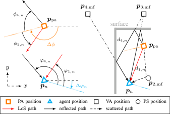
Figure 1: Geometrical depiction of a MIMO radio propagation environment, where MPCs are represented by MFs, e.g., VAs and PSs.

We consider a mmWave MIMO system operating in a dynamic scenario. For the sake of brevity, we assume a two-dimensional scenario with horizontal-only signal propagation. At each discrete time $n$, a PA with known position $\bm{p}_{\mathrm{pa}}=[p_{\mathrm{pa},\mathrm{x}}\hskip 2.84526ptp_{\mathrm{pa},\mathrm{y}}]^{\mathrm{T}}$ transmits a radio signal and a mobile agent at unknown time-varying position $\bm{p}_{n}=[p_{n,\mathrm{x}}\hskip 2.84526ptp_{n,\mathrm{y}}]^{\mathrm{T}}$ acts as a receiver. We assume time and frequency synchronization between the PA and the mobile agent. The PA is equipped with a $N_{\mathrm{tx}}$-element antenna array with known orientation $\Delta\phi$, and the mobile agent is equipped with a $N_{\mathrm{rx}}$-element antenna array with unknown azimuth orientation $\Delta\varphi_{n}$, respectively. The positions $\bm{p}_{\mathrm{pa}}$ and $\bm{p}_{n}$ refer to the center of gravity of the arrays. Specularly reflected MPCs and scattered MPCs can be modeled by VAs and PSs, reflectively. The PA, VAs and PSs are collectively referred to as MFs at unknown but fixed positions $\bm{p}_{l,\mathrm{mf}}=[p_{l,\mathrm{mf},\mathrm{x}}\hskip 2.84526ptp_{l,\mathrm{mf},\mathrm{y}}]^{\mathrm{T}}$, with $l\in\{1,\dots,L_{n}\}$.

As shown in Fig. 1, for MPCs generated by VA-type of MFs, the propagation distances and AoAs at time $n$ are given by $d_{l,n}=\mathrm{d}_{\mathrm{va}}(\bm{p}_{n},\bm{p}_{l,\mathrm{mf}})$ and $\varphi_{l,n}=\angle(\bm{p}_{n},\bm{p}_{l,\mathrm{mf}},\Delta\varphi_{n})$, respectively. For MPCs originated from PS-type of MFs, the propagation distances, AoAs, and AoDs are given by $d_{l,n}=\mathrm{d}_{\mathrm{ps}}(\bm{p}_{n},\bm{p}_{l,\mathrm{mf}},\bm{p}_{\mathrm{pa}})$, $\varphi_{l,n}=\angle(\bm{p}_{n},\bm{p}_{l,\mathrm{mf}},\Delta\varphi_{n})$ and $\phi_{l,n}=\angle(\bm{p}_{l,\mathrm{mf}},\bm{p}_{\mathrm{pa}},\Delta\phi)$. To conveniently address the PA-related variables and factors, we define $\bm{p}_{1,\mathrm{mf}}\triangleq\bm{p}_{\mathrm{pa}}$.

III Radio Signal Model and Channel Estimation

III-A Discrete-Frequency Signal Model

The received signals are sampled with frequency spacing $\Delta B$ over the bandwidth $B$, yielding a length $N_{\mathrm{f}}=B/\Delta B$ sample vector for each PA and mobile agent antenna pair. By stacking the samples from all $N_{\mathrm{rx}}N_{\mathrm{tx}}$ antenna pairs, we obtain the discrete-frequency signal vector $\bm{r}_{n}\in\mathbb{C}^{N_{\mathrm{rx}}N_{\mathrm{tx}}N_{\mathrm{f}}\times 1}$

$$\bm{r}_{n}=\sum_{l=1}^{L_{n}}\bm{B}(\bm{\theta}_{l,n})\bm{\alpha}_{l,n}+\bm{n}_{n}$$ (1)

where the first term comprises $L_{n}$ MPCs, with each characterized by its state vector $\bm{\theta}_{l,n}\triangleq\big{[}d_{l,n}\hskip 2.84526pt\phi_{l,n}\hskip 2.84526pt\varphi_{l,n}\big{]}^{\mathrm{T}}$ containing the delay $\tau_{l,n}=d_{l,n}/c$, AoD $\phi_{l,n}$, AoA $\varphi_{l,n}$, and complex amplitude $\bm{\alpha}_{l,n}\triangleq[\alpha_{\mathrm{hh},l,n}\hskip 2.84526pt\alpha_{\mathrm{hv},l,n}\hskip 2.84526pt\alpha_{\mathrm{vh},l,n}\hskip 2.84526pt\alpha_{\mathrm{vv},l,n}]^{\mathrm{T}}$. We define the matrix $\bm{B}(\bm{\theta}_{l,n})\triangleq\big{[}\bm{b}_{\mathrm{hh}}(\bm{\theta}_{l,n})\hskip 2.84526pt\bm{b}_{\mathrm{hv}}(\bm{\theta}_{l,n})\hskip 2.84526pt\bm{b}_{\mathrm{vh}}(\bm{\theta}_{l,n})\hskip 2.84526pt\bm{b}_{\mathrm{vv}}(\bm{\theta}_{l,n})\big{]}\in\mathbb{C}^{N_{\mathrm{rx}}N_{\mathrm{tx}}N_{\mathrm{f}}\times 4}$ with columns given by $\bm{b}_{\mathrm{hv}}(\bm{\theta}_{l,n})\triangleq\mathrm{reshape}\big{(}\bm{b}_{\mathrm{rx},\mathrm{h}}(\varphi_{l,n})\lozenge\bm{b}_{\mathrm{tx},\mathrm{v}}(\phi_{l,n})\lozenge\bm{b}_{\mathrm{f}}^{\mathrm{T}}(\tau_{l,n})\big{)}\in\mathbb{C}^{N_{\mathrm{rx}}N_{\mathrm{tx}}N_{\mathrm{f}}\times 1}$ and $\lozenge$ denotes the Khatri–Rao product. The vectors $\bm{b}_{\mathrm{rx},\mathrm{h}}(\varphi_{l,n})\in\mathbb{C}^{N_{\mathrm{rx}}\times N_{\mathrm{f}}}$ and $\bm{b}_{\mathrm{tx},\mathrm{v}}(\phi_{l,n})\in\mathbb{C}^{N_{\mathrm{tx}}\times N_{\mathrm{f}}}$ represent the far-field complex array responses by using the effective aperture distribution function (EADF) [10], and $\bm{b}_{\mathrm{f}}(\tau_{l,n})\in\mathbb{C}^{N_{\mathrm{f}}\times 1}$ accounts for the system response, baseband signal spectrum and the phase shift due to delay $\tau_{l,n}$ [11]. The measurement noise vector $\bm{n}_{n}\in\mathbb{C}^{N_{\mathrm{rx}}N_{\mathrm{tx}}N_{\mathrm{f}}\times 1}$ is a zero-mean, complex circular symmetric Gaussian random vector with covariance matrix $\bm{C}=\sigma^{2}\bm{I}_{N_{\mathrm{rx}}N_{\mathrm{tx}}N_{\mathrm{f}}}$ where $\sigma^{2}$ is the noise variance. The MPC SNR is given as the SNR calculated for $\mathrm{hh}$ transmission, i.e., $\mathrm{SNR}_{l,n}=\frac{|\alpha_{\mathrm{hh},l,n}|^{2}\lVert\bm{b}_{\mathrm{hh}}(\bm{\theta}_{l,n})\rVert^{2}}{\sigma^{2}}$ and the according normalized amplitude is $u_{l,n}=\sqrt{\mathrm{SNR}_{l,n}}$.

III-B Parametric Channel Estimation

Based on the signal model in (1), a snapshot-based parametric channel estimation algorithm SAGE is applied in the pre-estimation stage[12], providing estimated dispersion parameters of $M_{n}$ MPCs stacked into the vector $\bm{z}_{n}\triangleq[\bm{z}_{1,n}^{\mathrm{T}}\hskip 0.85358pt\cdots\hskip 0.85358pt\bm{z}_{M_{n},n}^{\mathrm{T}}]^{\mathrm{T}}\in\mathbb{R}^{4M_{n}\times 1}$. Each $\bm{z}_{m,n}\triangleq[{z_{\mathrm{d}}}_{m,n}\hskip 2.84526pt{z_{\mathrm{\phi}}}_{m,n}\hskip 2.84526pt{z_{\mathrm{\varphi}}}_{m,n}\hskip 2.84526pt{z_{\mathrm{u}}}_{m,n}]^{\mathrm{T}}$ comprises estimates ${z_{\mathrm{d}}}_{m,n}$ of the distance, the estimates ${z_{\mathrm{\phi}}}_{m,n}$ of the AoD, the estimates ${z_{\mathrm{\varphi}}}_{m,n}$ of the AoA, and the estimates ${z_{\mathrm{u}}}_{m,n}\in[u_{\mathrm{de}},\infty)$ of normalized amplitude, as well as of the noise variance. The estimates $\bm{z}_{n}$ above the detection threshold $u_{\mathrm{de}}$ are used as noisy measurements by the proposed algorithm.

IV System model

IV-A Agent State and PMF States

At each time $n$, the state of mobile agent is given by $\bm{\mathsfbr{x}}_{n}\triangleq[\bm{\mathsfbr{p}}_{n}^{\mathrm{T}}\hskip 2.84526pt\bm{\mathsfbr{v}}_{n}^{\mathrm{T}}]^{\mathrm{T}}$ consisting of the position $\bm{\mathsfbr{p}}_{n}$ and the velocity $\bm{\mathsfbr{v}}_{n}=[\mathsfbr{v}_{\mathrm{x},n}\hskip 2.84526pt\mathsfbr{v}_{\mathrm{y},n}]^{\mathrm{T}}$. We assume that the array of the mobile agent is rigidly coupled with the movement direction, i.e., azimuth array orientation $\mathsfbr{{\Delta\varphi}}_{n}$ is determined by the direction of its velocity vector $\bm{\mathsfbr{v}}_{n}$, i.e., ${\Delta\varphi}_{n}(\bm{v}_{n})=\mathrm{atan2}(\frac{v_{\mathrm{y},n}}{v_{\mathrm{x},n}})$. All agent states up to time $n$ are denoted as $\bm{\mathsfbr{x}}_{1:n}\triangleq[\bm{\mathsfbr{x}}_{1}^{\mathrm{T}}\hskip 0.85358pt\cdots\hskip 0.85358pt\bm{\mathsfbr{x}}_{n}^{\mathrm{T}}]^{\mathrm{T}}$.

Following [1, 2], we account for the unknown and time-varying number of MFs by introducing potential s indexed by $k\in\{1,\dots,K_{n}\}$, where $K_{n}$ represents the maximum possible number of MFs that produced a measurement so far and $K_{n}$ increases with time. Augmented states of PMFs are denoted as $\bm{\mathsfbr{y}}_{k,n}\triangleq[\bm{\mathsfbr{{\mu}}}_{k,n}^{\mathrm{T}}\hskip 2.84526pt\mathsfbr{r}_{k,n}]^{\mathrm{T}}$ with $\bm{\mathsfbr{{\mu}}}_{k,n}=[\bm{\mathsfbr{p}}^{\mathrm{T}}_{k,\mathrm{mf}}\hskip 2.84526pt\mathsfbr{u}_{k,n}]^{\mathrm{T}}$. The existence/non-existence of the $k$th PMF is modeled by a binary random variable $\mathsfbr{r}_{k,n}\in\{0,1\}$ in the sense that it exists if and only if $r_{k,n}=1$. The type of the $k$th PMF is modeled by a random variable $\mathsfbr{q}_{k,n}\in\{1,2\}$ in the sense that the $k$th PMF is a VA-type of MF if $q_{k,n}=1$ and it is a PS-type of MF if $q_{k,n}=2$. Formally, PMF $k$ is also considered even if it is non-existent, i.e., $r_{k,n}=0$. The states $\bm{\mathsfbr{{\mu}}}_{k,n}$ of non-existent PMFs are obviously irrelevant and have no influence on the PMF detection and state estimation. Therefore, all probability density functions defined for PMF states $f(\bm{\mathsfbr{y}}_{k,n})=f(\bm{\mathsfbr{{\mu}}}_{k,n},\mathsfbr{r}_{k,n})$ are of the form $f(\bm{\mathsfbr{{\mu}}}_{k,n},0)=f_{k,n}f_{\mathrm{D}}(\bm{\mathsfbr{{\mu}}}_{k,n})$, where $f_{\mathrm{D}}(\bm{\mathsfbr{{\mu}}}_{k,n})$ is an arbitrary “dummy PDF” and $f_{k,n}\in[0,1]$ is a constant representing the probability of nonexistence [13, 14, 1].

IV-B Measurement Model

Before the measurements are observed, they are considered as random and denoted as $\bm{\mathsfbr{z}}_{n}\triangleq[\bm{\mathsfbr{z}}_{1,n}^{\mathrm{T}}\hskip 0.85358pt\cdots\hskip 0.85358pt\bm{\mathsfbr{z}}_{M_{n},n}^{\mathrm{T}}]^{\mathrm{T}}\in\mathbb{R}^{4\mathsfbr{M}_{n}\times 1}$ and $\bm{\mathsfbr{z}}_{m,n}\triangleq[{\mathsfbr{z}_{\mathrm{d}}}_{m,n}\hskip 2.84526pt{\mathsfbr{z}_{\mathrm{\phi}}}_{m,n}\hskip 2.84526pt{\mathsfbr{z}_{\mathrm{\varphi}}}_{m,n}\hskip 2.84526pt{z_{\mathrm{u}}}_{m,n}]^{\mathrm{T}}$. An existing PMF generates a PMF-originated measurement $\bm{\mathsfbr{z}}_{m,n}$ with detection probability ${p_{\mathrm{d}}}(\mathsfbr{u}_{k,n})$ corresponding to the normalized amplitude $\mathsfbr{u}_{k,n}$. The measurement likelihood function (LHF) is assumed to be conditionally independent across the individual measurements within the vector $\bm{\mathsfbr{z}}_{m,n}$. The individual LHFs of the distance, AoA and AoD measurements are modeled by Gaussian PDFs. More specifically, the LHFs of the distance measurements for VA-originated and PS-originated paths are given by

$$f_{q_{k,n}=1}({z_{\mathrm{d}}}_{m,n}|\bm{p}_{n},\bm{{\mu}}_{k,n})$$

$$\hskip 22.76219pt=f_{\mathrm{N}}({z_{\mathrm{d}}}_{m,n};\mathrm{d}_{\mathrm{va}}(\bm{p}_{n},\bm{p}_{k,\mathrm{mf}}),\sigma_{\mathrm{d}}^{2}(u_{k,n})),$$ (2)

$$f_{q_{k,n}=2}({z_{\mathrm{d}}}_{m,n}|\bm{p}_{n},\bm{{\mu}}_{k,n},\bm{p}_{1,\mathrm{mf}})$$

$$\hskip 22.76219pt=f_{\mathrm{N}}({z_{\mathrm{d}}}_{m,n};\mathrm{d}_{\mathrm{ps}}(\bm{p}_{n},\bm{p}_{k,\mathrm{mf}},\bm{{p}}_{1,\mathrm{mf}}),\sigma_{\mathrm{d}}^{2}(u_{k,n})),$$ (3)

respectively. The LHFs of the AoD measurements for the LoS path are given by

$$f({z_{\mathrm{\phi}}}_{m,n}|\bm{{p}}_{1,\mathrm{mf}},\bm{p}_{n},u_{k,n})$$

$$\hskip 22.76219pt=f_{\mathrm{N}}({z_{\mathrm{\phi}}}_{m,n};\angle(\bm{{p}}_{1,\mathrm{mf}},\bm{p}_{n},\Delta\phi),\sigma_{\mathrm{\phi}}^{2}(u_{k,n})).$$ (4)

The LHFs of the AoD measurements for PS-originated path are given by

$$f({z_{\mathrm{\phi}}}_{m,n}|\bm{{p}}_{1,\mathrm{mf}},\bm{{\mu}}_{k,n})$$

$$\hskip 22.76219pt=f_{\mathrm{N}}({z_{\mathrm{\phi}}}_{m,n};\angle(\bm{{p}}_{1,\mathrm{mf}},\bm{p}_{k,\mathrm{mf}},\Delta\phi),\sigma_{\mathrm{\phi}}^{2}(u_{k,n})).$$ (5)

The LHFs of the AoA measurements are given by

$$f({z_{\mathrm{\varphi}}}_{m,n}|\bm{x}_{n},\bm{{\mu}}_{k,n})$$

$$\hskip 22.76219pt=f_{\mathrm{N}}({z_{\mathrm{\varphi}}}_{m,n};\angle(\bm{p}_{n},\bm{p}_{k,\mathrm{mf}},\Delta\varphi(\bm{v}_{n})),\sigma_{\mathrm{\varphi}}^{2}(u_{k,n})).$$ (6)

The variances ${\sigma_{\mathrm{d}}}^{2}(u_{k,n})$, $\sigma_{\mathrm{\phi}}^{2}(u_{k,n})$ and $\sigma_{\mathrm{\varphi}}^{2}(u_{k,n})$ depend on the normalized amplitude $u_{k,n}$ and are determined based on the Fisher information given as ${\sigma_{\mathrm{d}}}^{2}(u_{k,n})=c^{2}/(8\pi^{2}\beta_{\mathrm{bw}}^{2}u_{k,n}^{2})$, $\sigma_{\phi_{k,n}}^{2}(u_{k,n})=c^{2}/(8\pi^{2}f_{\mathrm{c}}^{2}u_{k,n}^{2}D^{2}(\phi_{k,n}))$ and $\sigma_{\varphi_{k,n}}^{2}(u_{k,n})=c^{2}/(8\pi^{2}f_{\mathrm{c}}^{2}u_{k,n}^{2}D^{2}(\varphi_{k,n}))$ with $\beta_{\mathrm{bw}}^{2}$ denoting the mean square bandwidth of the transmit signal pulse and $D^{2}(\cdot)$ is the squared array aperture [15, 9].

The LHFs of the normalized amplitude measurements $u_{k,n}>u_{\mathrm{de}}$ is modeled by a truncated Rician PDF [16, Ch. 1.6.7][17], i.e.,

$$f({z_{\mathrm{u}}}_{m,n}|u_{k,n})=f_{\mathrm{R}}({z_{\mathrm{u}}}_{m,n};u_{k,n},\sigma_{\mathrm{u}}(u_{k,n}),{p_{\mathrm{d}}}(u_{k,n});u_{\mathrm{de}})$$ (7)

where the scale parameter $\sigma_{\mathrm{u}}(u_{k,n})$ corresponding to $u_{k,n}$ is determined based on the Fisher information given as $\sigma_{\mathrm{u}}^{2}(u_{k,n})=\frac{1}{2}+\frac{1}{4N_{\mathrm{rx}}N_{\mathrm{tx}}N_{\mathrm{f}}}u_{k,n}^{2}$. The detection probability ${p_{\mathrm{d}}}(u_{k,n})$ is modeled by the Marcum Q-function, i.e., ${p_{\mathrm{d}}}(u_{k,n})=Q_{1}(u_{k,n}/{\sigma_{\mathrm{u}}}_{k,n},u_{\mathrm{de}}/{\sigma_{\mathrm{u}}}_{k,n})$ [16, 17].

Using (2) to (7), the LHFs $f_{q_{k,n}}(\bm{z}_{m,n}|\bm{x}_{n},\bm{{\mu}}_{k,n},\bm{{\mu}}_{1,n})$ for measurements originated from different type of PMFs are given as follows.

IV-B1 LHF for VA-originated path

The LHF for VA-originated paths is $f_{q_{k,n}=1}(\bm{z}_{m,n}|\bm{x}_{n},\bm{{\mu}}_{k,n})$, which factorizes as

$$f_{q_{k,n}=1}(\bm{z}_{m,n}|\bm{x}_{n},\bm{{\mu}}_{k,n}) =f_{q_{k,n}=1}({z_{\mathrm{d}}}_{m,n}|\bm{p}_{n},\bm{{\mu}}_{k,n})$$

$$\times f({z_{\mathrm{\varphi}}}_{m,n}|\bm{x}_{n},\bm{{\mu}}_{k,n})f({z_{\mathrm{u}}}_{m,n}|u_{k,n}).$$ (8)

Note that the LoS path is considered as a VA-originated path, but the corresponding LHF also accounts for the AoD measurement, yields

$$f_{q_{k,n}=1}(\bm{z}_{m,n}|\bm{x}_{n},\bm{{\mu}}_{1,n})$$

$$\hskip 5.69054pt=f_{q_{k,n}=1}({z_{\mathrm{d}}}_{m,n}|\bm{p}_{n},\bm{{\mu}}_{1,n})f({z_{\mathrm{\phi}}}_{m,n}|\bm{p}_{1,\mathrm{mf}},\bm{p}_{n},u_{1,n})$$

$$\hskip 5.69054pt\times f({z_{\mathrm{\varphi}}}_{m,n}|\bm{x}_{n},\bm{{\mu}}_{1,n})f({z_{\mathrm{u}}}_{m,n}|u_{1,n})$$ (9)

IV-B2 LHF for PS-originated path

$$f_{q_{k,n}=2}(\bm{z}_{m,n}|\bm{x}_{n},\bm{{\mu}}_{k,n},\bm{{\mu}}_{1,n})$$

$$=f_{q_{k,n}=2}({z_{\mathrm{d}}}_{m,n}|\bm{p}_{n},\bm{{\mu}}_{k,n},\bm{p}_{1,\mathrm{mf}})f({z_{\mathrm{\phi}}}_{m,n}|\bm{p}_{n},\bm{{\mu}}_{k,n})$$

$$\hskip 5.69054pt\times f({z_{\mathrm{\varphi}}}_{m,n}|\bm{x}_{n},\bm{{\mu}}_{k,n})f({z_{\mathrm{u}}}_{m,n}|u_{k,n})$$ (10)

IV-B3 LHF for FAs

We assume that the false alarm (FA) measurements originating from the snapshot-based parametric channel estimator are statistically independent of PMF states. They are modeled by a Poisson point process with mean number $\mu_{\mathrm{fa}}$ and PDF $f_{\mathrm{fa},q_{k,n}}(\bm{z}_{m,n})$. For VA-originated paths, the FA PDF is factorized as $f_{\mathrm{fa},q_{k,n}=1}(\bm{z}_{m,n})=f_{\mathrm{fa}}({z_{\mathrm{d}}}_{m,n})f_{\mathrm{fa}}({z_{\mathrm{\varphi}}}_{m,n})f_{\mathrm{fa}}({z_{\mathrm{u}}}_{m,n})$. For LoS path and PS-originated paths, the PDF is factorized as $f_{\mathrm{fa},q_{k,n}=2}(\bm{z}_{m,n})=f_{\mathrm{fa}}({z_{\mathrm{d}}}_{m,n})f_{\mathrm{fa}}({z_{\mathrm{\phi}}}_{m,n})f_{\mathrm{fa}}({z_{\mathrm{\varphi}}}_{m,n})f_{\mathrm{fa}}({z_{\mathrm{u}}}_{m,n})$. The LHFs of FA measurements corresponding to distance, azimuth angle and elevation angle are uniformly distributed on $[0,d_{\mathrm{max}}]$, $[-\pi,\pi)$ and $[0,\pi]$, respectively. The false alarm LHF $f_{\mathrm{fa}}({z_{\mathrm{u}}}_{m,n})$ of the normalized amplitude is given by a truncated Rayleigh PDF (see [17, 18] for details).

IV-C State-Transition Model

For each PMF with state $\bm{\mathsfbr{y}}_{k,n-1}$ with $k\in\{1,\dots,K_{n-1}\}$ at time $n-1$, there is one “legacy” PMF with state $\underline{\bm{\mathsfbr{y}}}_{k,n}\triangleq[\underline{\bm{\mathsfbr{{\mu}}}}_{k,n}^{\mathrm{T}}\hskip 2.84526pt\underline{\mathsfbr{r}}_{k,n}]^{\mathrm{T}}$ with $k\in\{1,\dots,K_{n-1}\}$ at time $n$. We define the stacked PMF state vector $\underline{\bm{\mathsfbr{y}}}_{n}\triangleq[\underline{\bm{\mathsfbr{y}}}_{1,n}^{\mathrm{T}}\hskip 0.85358pt\cdots\hskip 0.85358pt\underline{\bm{\mathsfbr{y}}}_{K_{n-1},n}^{\mathrm{T}}]^{\mathrm{T}}$ and stacked PMF type state vector $\underline{\bm{\mathsfbr{q}}}_{n}=[\underline{\mathsfbr{q}}_{1,n}\hskip 0.85358pt\cdots\hskip 0.85358pt\underline{\mathsfbr{q}}_{K_{n-1},n}]^{\mathrm{T}}$. Following the interacting multiple model (IMM) approach, the temporal evolution of PMF type index $\mathsfbr{q}_{k,n}$ is modeled by a discrete Markov chain with constant transition matrix $\bm{Q}\in[0,1]^{2\times 2}$ over time, and the transition probability mass function (PMF) is given by $p(\underline{q}_{k,n}=1|q_{k,n}=2)=[\bm{Q}]_{2,1}$ with $\sum_{i=1}^{2}[\bm{Q}]_{i^{\prime},i}=1\hskip 2.84526pt\forall\hskip 2.84526pti^{\prime}$ . The PMF type index is assumed to evolve independently across $k$ and $n$, this the factorized prior PMF of joint state is given as

$$p(\underline{\bm{q}}_{n}|\bm{q}_{n-1})=\prod_{k=1}^{K_{n-1}}p(\underline{q}_{k,n}|q_{k,n-1})$$ (11)

where $p(\bm{q}_{0})$ is the initial PMF type PMF at time $n=0$. The agent state and the legacy PMFs states are assumed to evolve independently across $k$ and $n$ according to state-transition PDFs $f(\bm{x}_{n}|\bm{x}_{n-1})$ and $f(\underline{\bm{y}}_{k,n}|\bm{y}_{k,n-1})$, respectively, yields

$$f(\bm{x}_{n},\underline{\bm{y}}_{n}|\bm{x}_{n-1},\bm{y}_{n-1})=f(\bm{x}_{n}|\bm{x}_{n-1})\prod_{k=1}^{K_{n-1}}f(\underline{\bm{y}}_{k,n}|\bm{y}_{k,n-1})$$ (12)

where the formulation of the augmented PMF state-transition PDF $f(\underline{\bm{y}}_{k,n}|\bm{y}_{k,n-1})=f(\underline{\bm{\mu}}_{k,n},\underline{r}_{k,n}|\bm{\mu}_{k,n-1},r_{k,n-1})$ is inline with [13, 1].

IV-D New PMFs

Newly detected MFs at time $n$, i.e., PMFs that generate measurements for the first time at time $n$, are modeled by a Poisson point process with mean $\mu_{\mathrm{n}}$ and PDF $f_{\mathrm{n}}(\overline{\bm{\mu}}_{m,n})$. Following [13, 1], newly detected PMFs are represented by new PMF states $\overline{\bm{\mathsfbr{y}}}_{m,n}\triangleq[\overline{\bm{\mathsfbr{x}}}_{m,n}^{\mathrm{T}}\hskip 2.84526pt\overline{\mathsfbr{r}}_{m,n}]^{\mathrm{T}}$, $m\in\{1,\dots,\mathsfbr{M}_{n}\}$. Each new PMF $\overline{\bm{\mathsfbr{y}}}_{m,n}$ corresponds to a measurement $\bm{\mathsfbr{z}}_{m,n}$, and $\overline{r}_{m,n}=1$ means that the measurement $\bm{\mathsfbr{z}}_{m,n}$ was generated by a newly detected PMF. The state vector of all new PMFs at time $n$ is given by $\overline{\bm{\mathsfbr{y}}}_{n}\triangleq[\overline{\bm{\mathsfbr{y}}}_{1,n}^{\mathrm{T}}\hskip 0.85358pt\cdots\hskip 0.85358pt\overline{\bm{\mathsfbr{y}}}_{\mathsfbr{M}_{n},n}^{\mathrm{T}}]^{\mathrm{T}}$ and the stacked PMF type state vector is given by $\overline{\bm{\mathsfbr{q}}}_{n}=[\overline{\mathsfbr{q}}_{1,n}\hskip 0.85358pt\cdots\hskip 0.85358pt\overline{\mathsfbr{q}}_{\mathsfbr{M}_{n},n}]^{\mathrm{T}}$. The new PMFs $\overline{\bm{\mathsfbr{y}}}_{n}$ become legacy PMFs at time $n+1$, accordingly the number of legacy PMFs is updated as $K_{n}=K_{n-1}+M_{n}$. We also define $\bm{\mathsfbr{y}}_{n}\triangleq[\underline{\bm{\mathsfbr{y}}}_{n}^{\mathrm{T}}\hskip 2.84526pt\overline{\bm{\mathsfbr{y}}}_{n}^{\mathrm{T}}]^{\mathrm{T}}$ with $\bm{\mathsfbr{y}}_{k,n}$ and $k\in\{1,\dots,K_{n}\}$, and $\bm{\mathsfbr{q}}_{n}\triangleq[\underline{\bm{\mathsfbr{q}}}_{n}^{\mathrm{T}}\hskip 2.84526pt\overline{\bm{\mathsfbr{q}}}_{n}^{\mathrm{T}}]^{\mathrm{T}}$. The state and type vectors for all times up to $n$ are given by $\bm{\mathsfbr{y}}_{1:n}\triangleq[\bm{\mathsfbr{y}}_{1}^{\mathrm{T}}\hskip 0.85358pt\cdots\hskip 0.85358pt\bm{\mathsfbr{y}}_{n}^{\mathrm{T}}]^{\mathrm{T}}$ and $\bm{\mathsfbr{q}}_{1:n}\triangleq[\bm{\mathsfbr{q}}_{1}^{\mathrm{T}}\hskip 0.85358pt\cdots\hskip 0.85358pt\bm{\mathsfbr{q}}_{n}^{\mathrm{T}}]^{\mathrm{T}}$, respectively.

IV-E Data Association

Estimation of multiple PMF states is complicated by the data association (DA) uncertainty. Furthermore, it is not known if a measurement did not originate from a PMF (false alarm), or if a PMF did not generate any measurement (missed detection). The associations between measurements and legacy PMFs are described by the PMF-oriented association vector $\bm{\mathsfbr{\underline{a}}}_{n}\triangleq[\mathsfbr{\underline{a}}_{1,n}\hskip 0.85358pt\cdots\hskip 0.85358pt\mathsfbr{\underline{a}}_{\mathsfbr{K}_{n-1},n}]^{\mathrm{T}}$ with entries $\mathsfbr{\underline{a}}_{k,n}\triangleq m\in\{1,\dots,\mathsfbr{M}_{n}\}$, if legacy PMF $k$ generates measurement $m$, or $\mathsfbr{\underline{a}}_{k,n}\triangleq 0$, if legacy PMF $k$ does not generate any measurement. In line with [19, 13, 1], the associations can be equivalently described by a measurement-oriented association vector $\bm{\mathsfbr{\overline{a}}}_{n}\triangleq[\mathsfbr{\overline{a}}_{1,n}\hskip 0.85358pt\cdots\hskip 0.85358pt\mathsfbr{\overline{a}}_{\mathsfbr{M}_{n},n}]^{\mathrm{T}}$ with entries $\mathsfbr{\overline{a}}_{m,n}\triangleq k\in\{1,\dots,K_{n-1}\}$, if measurement $m$ is generated by legacy PMF $k$, or $\mathsfbr{\overline{a}}_{m,n}\triangleq 0$, if measurement $m$ is not generated by any legacy PMF. Furthermore, we assume that at any time $n$, each PMF can generate at most one measurement, and each measurement can be generated by at most one PMF [19, 13, 1]. The “redundant formulation” of using $\bm{\mathsfbr{\underline{a}}}_{n}$ together with $\bm{\mathsfbr{\overline{a}}}_{n}$ is the key to make the algorithm scalable for large numbers of PMFs and measurements. The association vectors for all times up to $n$ are given by $\bm{\mathsfbr{\underline{a}}}_{1:n}\triangleq[\bm{\mathsfbr{\underline{a}}}_{1}^{\mathrm{T}}\hskip 0.85358pt\cdots\hskip 0.85358pt\bm{\mathsfbr{\underline{a}}}_{n}^{\mathrm{T}}]^{\mathrm{T}}$ and $\bm{\mathsfbr{\overline{a}}}_{1:n}\triangleq[\bm{\mathsfbr{\overline{a}}}_{1}^{\mathrm{T}}\hskip 0.85358pt\cdots\hskip 0.85358pt\bm{\mathsfbr{\overline{a}}}_{n}^{\mathrm{T}}]^{\mathrm{T}}$.

IV-F Joint Posterior PDF

By using common assumptions [16, 13, 1], the joint posterior PDF of $\bm{\mathsfbr{x}}_{0:n}$, $\bm{\mathsfbr{y}}_{0:n}$, $\bm{\mathsfbr{q}}_{1:n}$, $\bm{\mathsfbr{\underline{a}}}_{1:n}$ and $\bm{\mathsfbr{\overline{a}}}_{1:n}$ conditioned on observed (thus fixed) measurements $\bm{z}_{1:n}$ is given by

$$f(\bm{x}_{0:n},\bm{y}_{0:n},\bm{q}_{0:n},\bm{\underline{a}}_{1:n},\bm{\overline{a}}_{1:n}|\bm{z}_{1:n})$$

$$\propto\left(f(\bm{x}_{0})\prod_{i=1}^{K_{0}}f(\bm{y}_{i,0})f(q_{i,0})\right)\prod_{n^{\prime}=1}^{n}f(\bm{x}_{n^{\prime}}|\bm{x}_{n^{\prime}-1})$$

$$\times\left(\prod_{k^{\prime}=1}^{K_{n^{\prime}-1}}f(\underline{\bm{y}}_{k^{\prime},n^{\prime}}|\bm{y}_{k^{\prime},n^{\prime}-1})p(\underline{q}_{k^{\prime},n^{\prime}}|q_{k^{\prime},n^{\prime}-1})\right)$$

$$\times\left(\prod_{k=1}^{K_{n^{\prime}-1}}g(\underline{\bm{y}}_{k,n^{\prime}},\underline{q}_{k^{\prime},n^{\prime}},\underline{a}_{k,n^{\prime}},\bm{x}_{n^{\prime}};\bm{z}_{n^{\prime}})\prod_{m=1}^{M_{n^{\prime}}}\psi(\underline{a}_{k,n^{\prime}},\overline{a}_{m,n^{\prime}})\right)$$

$$\times\left(\prod_{m^{\prime}=1}^{M_{n^{\prime}}}h(\overline{\bm{y}}_{m^{\prime},n^{\prime}},\overline{q}_{m^{\prime},n^{\prime}},\overline{a}_{m^{\prime},n^{\prime}},\bm{x}_{n^{\prime}};\bm{z}_{m,n^{\prime}})\right)$$ (13)

where the pseudo LHFs $g(\underline{\bm{y}}_{k,n},\underline{q}_{k,n},\underline{a}_{k,n},\bm{x}_{n};\bm{z}_{n})=g(\underline{\bm{\mu}}_{k,n},\\ \underline{r}_{k,n},\underline{q}_{k,n},\underline{a}_{k,n},\bm{x}_{n};\bm{z}_{n})$ related to legacy PMFs are given by

$$g(\underline{\bm{\mu}}_{k,n},\underline{r}_{k,n}=1,\underline{q}_{k,n},\underline{a}_{k,n},\bm{x}_{n};\bm{z}_{n})$$

$$\triangleq\begin{cases}\dfrac{f_{q_{k,n}}(\bm{z}_{m,n}|\bm{x}_{n},\underline{\bm{\mu}}_{k,n},\underline{\bm{\mu}}_{1,n})p_{\mathrm{d}}(\underline{u}_{k,n})}{\mu_{\mathrm{fa}}f_{\mathrm{fa},q_{k,n}}(\bm{z}_{m,n})},&\underline{a}_{k,n}=m\\ 1-p_{\mathrm{d}}(\underline{u}_{k,n}),&\underline{a}_{k,n}=0\end{cases}$$ (14)

and $g(\underline{\bm{\mu}}_{k,n},\underline{r}_{k,n}=0,\underline{q}_{k,n},\underline{a}_{k,n},\bm{x}_{n};\bm{z}_{n})\triangleq\delta(\underline{a}_{k,n})$. The pseudo LHFs $h(\overline{\bm{y}}_{m,n},\overline{q}_{m,n},\overline{a}_{m,n},\bm{x}_{n};\bm{z}_{m,n})=h(\overline{\bm{\mu}}_{m,n},\\ \overline{r}_{m,n},\overline{q}_{m,n},\overline{a}_{m,n},\bm{x}_{n};\bm{z}_{m,n})$ related to new PMFs are given by

$$h(\overline{\bm{\mu}}_{m,n},\overline{r}_{m,n}=1,\overline{q}_{m,n},\overline{a}_{m,n},\bm{x}_{n};\bm{z}_{m,n})$$

$$\triangleq\begin{cases}0,&\overline{a}_{m,n}=k\\ \dfrac{\mu_{\mathrm{n}}f_{\mathrm{n}}(\overline{\bm{\mu}}_{m,n})f_{q_{k,n}}(\bm{z}_{m,n}|\bm{x}_{n},\overline{\bm{\mu}}_{m,n},\overline{\bm{\mu}}_{1,n})}{\mu_{\mathrm{fa}}f_{\mathrm{fa},q_{k,n}}(\bm{z}_{m,n})},&\overline{a}_{m,n}=0\end{cases}$$ (15)

and $h(\overline{\bm{\mu}}_{m,n},\overline{r}_{m,n}=0,\overline{q}_{m,n},\overline{a}_{m,n},\bm{x}_{n};\bm{z}_{m,n})\triangleq f_{\mathrm{D}}(\overline{\bm{\mu}}_{k,n})$. The detailed derivations of the joint posterior PDF, the binary check function $\psi(\underline{a}_{k,n},\overline{a}_{m,n})$ and the factor graph representation of (13) are in parts inline with [13, 1, 17].

V Problem Formulation and Proposed Method

Using all the measurements up to time $n$, we aim to sequentially detect PMFs and estimate their positions and and agent state. This relies on the marginal posterior existence probabilities $p(r_{k,n}=1|\bm{z}_{1:n})$, the marginal posterior PDFs $f(\bm{p}_{k,\mathrm{mf}}|r_{k,n}=1,\bm{z}_{1:n})$, $f(q_{k,n}|r_{k,n}=1,\bm{z}_{1:n})$ and $f(\bm{x}_{n}|\bm{z}_{1:n})$. More specifically, a PMF is detected if $p(r_{k,n}=1|\bm{z}_{1:n})>p_{\mathrm{de}}$, with $p_{\mathrm{de}}$ denoting the detection threshold. The agent state $\bm{\mathsfbr{x}}_{n}$, and the states $\bm{\mathsfbr{p}}_{k,\mathrm{mf}}$ and $\mathsfbr{q}_{k,n}$ of detected PMFs are estimated by means of the minimum mean-square error (MMSE) estimator [20], i.e.,

$$\hat{\bm{x}}_{n} \triangleq\int\bm{x}_{n}f(\bm{x}_{n}|\bm{z}_{1:n})\mathrm{d}\bm{x}_{n}\vspace*{-2mm}$$ (16)

$$\hat{\bm{p}}_{k,\mathrm{mf}} \triangleq\int\bm{p}_{k,\mathrm{mf}}f(\bm{p}_{k,\mathrm{mf}}|r_{k,n}=1,\bm{z}_{1:n})\mathrm{d}\bm{p}_{k,\mathrm{mf}}\vspace*{-2mm}$$ (17)

$$\hat{q}_{k,n} \triangleq\sum_{i\in\bm{Q}}if(q_{k,n}|\bm{z}_{1:n})\vspace{-1mm}$$ (18)

where $f(\bm{p}_{k,\mathrm{mf}}|r_{k,n}=1,\bm{z}_{1:n})=\sum_{q_{k,\mathrm{mf}}\in\{1,2\}}f(\bm{p}_{k,\mathrm{mf}},q_{k,n}|\\ r_{k,n}=1,\bm{z}_{1:n})$ Since the marginal posterior PDFs $f(\bm{x}_{n}|\bm{z}_{1:n})$, $p(r_{k,n}=1|\bm{z}_{1:n})$ and $f(\bm{p}_{k,\mathrm{mf}}|r_{k,n}=1,\bm{z}_{1:n})$ cannot be obtained analytically, we use a computationally efficient sequential particle-based message-passing implementation by means of sum-product algorithm rules to obtain approximations of these marginal posterior PDFs. As the number of PMFs grows with time $n$ (at each time by $K_{n}=K_{n-1}+M_{n}$), PMFs with $p(r_{k,n}=1|\bm{z}_{1:n})$ below a threshold $p_{\mathrm{pr}}$ are removed from the state space (“pruned”).

VI Experimental Results

The performance of the proposed algorithm is validated using both synthetic and real radio measurements, for which the following setup and parameters are commonly used.

VI-A Analysis Setup

The state-transition PDF $f(\bm{x}_{n}|\bm{x}_{n-1})$ of the agent is defined by a linear near constant-velocity motion model[16], given as $\bm{x}_{n}=\bm{F}\bm{x}_{n-1}+\bm{\Gamma}\bm{\nu}_{n}$, where the matrix $\bm{F}\in\mathbb{R}^{4\times 4}$ and $\bm{\Gamma}\in\mathbb{R}^{4\times 2}$ are chosen as in [16] with the sampling period $\Delta T$. The driving process $\bm{\nu}_{n}\in\mathbb{R}^{2\times 1}$ is iid across time $n$, zero-mean and Gaussian with covariance matrix $\sigma_{\mathrm{\nu}}^{2}\mathbf{I}_{2}$, $\mathbf{I}_{2}$ denotes a $2\times 2$ diagonal matrix and $\sigma_{\mathrm{\nu}}^{2}=0.0025\,$$\text{m}/\text{s}^{2}$ represents the average speed increment along $x$ or $y$ axis during $\Delta T$. The state-transition PDF of legacy PMFs $\underline{\bm{p}}_{k,\mathrm{mf}}$ is chosen to be $\underline{\bm{p}}_{k,\mathrm{mf}}=\bm{p}_{k,\mathrm{mf}}+{\bm{\epsilon}}_{k,n}$, where the noise ${\bm{\epsilon}}_{k,n}$ is iid across $k$ and $n$, zero-mean, and Gaussian with variance ${\underline{\sigma}_{\mathrm{p}}}_{k}^{2}\mathbf{I}_{2}$ and ${\underline{\sigma}_{\mathrm{p}}}_{k}=10^{-5}\,$m. The state-transition PDF of the normalized amplitude $\underline{\mathsfbr{u}}_{k,n}$ is chosen to be $\underline{u}_{k,n}=u_{k,n-1}+{\epsilon_{\mathrm{u}}}_{k,n}$, where the noise ${\epsilon_{\mathrm{u}}}_{k,n}$ is iid across $k$ and $n$, zero-mean, and Gaussian with variance $\sigma_{\mathrm{u}}^{2}(\underline{u}_{k,n})$. The PMF mode transition probabilities are chosen as $[\bm{Q}]_{1,1}=[\bm{Q}]_{2,2}=0.96$ and $[\bm{Q}]_{1,2}=[\bm{Q}]_{2,1}=0.04$.

We assume that the geometric environment information is not available as a prior. The samples for the initial agent state are drawn from a $4$-D uniform distribution centered at $[\bm{p}_{0}^{\mathrm{T}}\hskip 2.84526pt0\hskip 2.84526pt0]^{\mathrm{T}}$ where $\bm{p}_{0}$ is the true agent start position, and the support of position and velocity components are $[-0.2,0.2]\,$m and $[0.02,0.02]\,$m/s, respectively. The samples for the initial states $\bm{{\mu}}_{k,n}$ of a new PMF are drawn from a $4$-D Gaussia distribution with means $[{z_{\mathrm{d}}}_{m,n}\hskip 2.84526pt{z_{\mathrm{\phi}}}_{m,n}\hskip 2.84526pt{z_{\mathrm{\varphi}}}_{m,n}\hskip 2.84526pt{z_{\mathrm{u}}}_{m,n}]^{\mathrm{T}}$ and variances calculated using the amplitude measurements ${z_{\mathrm{u}}}_{m,n}$ (see Section IV-B). The mean number of new PMFs is $\mu_{\mathrm{n}}=0.1$, the probability of survival is $p_{\mathrm{s}}=0.999$, the detection and pruning threshold are $p_{\mathrm{de}}=0.5$ and $p_{\mathrm{pr}}=10^{-3}$, and the particle number is $200000$.

VI-B Synthetic Measurement Evaluation

First, we present the simulation results using fully synthetic measurements without involving the snapshot-based channel estimator. We synthesized $3$ MPCs with time-varying distances, angles and amplitudes according to the true agent positions over $100$ time steps obtained in the real measurement and three true MFs (one PS and two VAs) highlighted with dotted circle markers in Fig. 4c. Fig. 2 shows the two PMF mode beliefs of the three detected MFs, averaged over $20$ simulation runs. It can be seen that the first detected MF (associated with the highlighted PS in Fig. 4c) rapidly converged to the PS mode, and the other two detected MFs (associated with the highlighted VAs in Fig. 4c) rapidly converged to the VA mode.

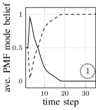
(a)

(b)

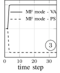
(c)

Figure 2: Results for synthetic measurements. Averaged PMF mode beliefs associated to the three true MFs highlighted in Fig. 4c.

VI-C Real Measurement Evaluation

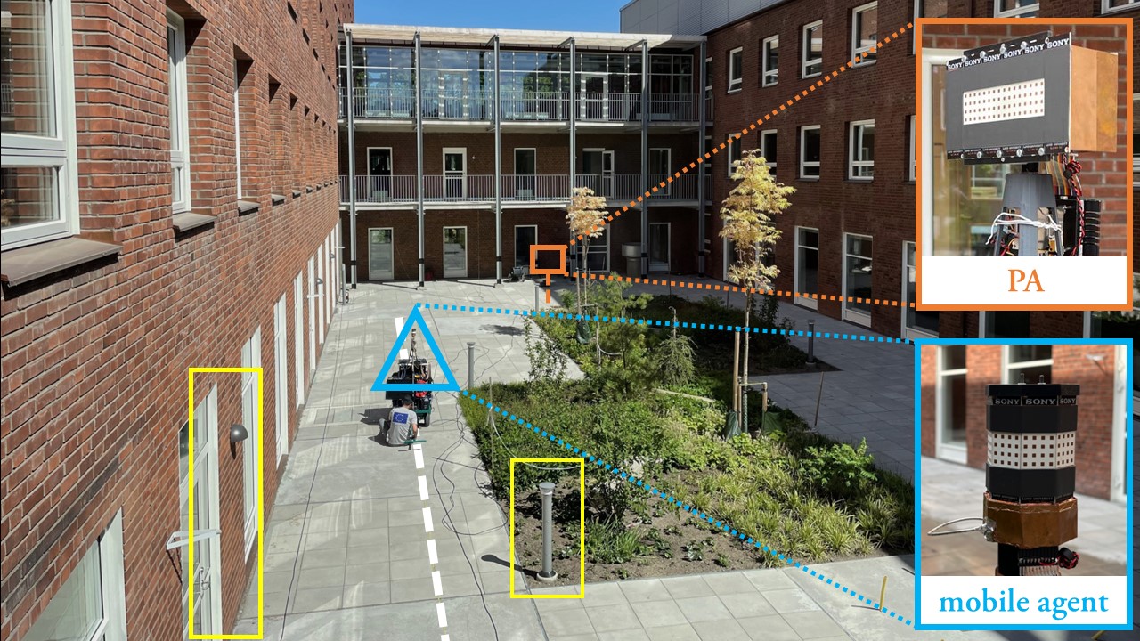
Figure 3: Overview of the measurement environment, Lund Sweden. The groud truth trajectory of the mobile agent is denoted with white dashed line. The static PA position and the current mobile agent position are indicated by a orange square and a cyan triangle, the same markers are also applied in Fig. 1 and Fig. 4c. A metallic pillar and a window corner are highlighted by yellow squares as examples of distinct point scatterers.

(a)

(b)

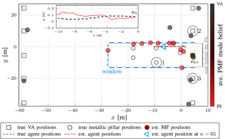
(c)

Figure 4: Performance results using real mmWave massive MIMO measurements. (a) RMSEs versus time of the agent position and (b) RMSEs versus time of the agent orientation. (c) shows the floorplan of the measurement environment (Fig. 3) including the windows, walls and true MF positions. The zoomed-in plot on the top shows the true and estimated agent positions. The MMSE estimates of detected MF positions at time $n=65$ are denoted as circle markers with the respective marker color representing the average of the two MF mode probability estimates. The three true MFs (one PS and two VAs) highlighted by dotted circles were used for generating the synthetic measurements in Section VI-B.

VI-C1 Measurement Setup

The performance is further validated using real mmWave massive MIMO measurements collected in a countyard at Lund University, Sweden, as shown in Fig. 3. The courtyard has approximate dimension of $35$ m$\times$$15$ m$\times$$13$ m, which presents a rich-scattering environment featuring vegetation and surrounded by brick walls with multiple reflective windows. The measurement used a switched array channel sounder supporting an effective bandwidth of $768$ MHz centered at $28$ GHz. On the PA side, a uniform planar array with $64$ dual-polarized patch antennas ($128$ ports in total) was placed at a fixed known position with the main radiation direction facing the yard. At the mobile agent side, a cylindrical array with $128$ dual-polarized patch antennas ($256$ ports in total) was used and manually moved along a $10\,$m straight line trajectory. The channel impulse response was recorded every $10\,$cm, generating a total of $100$ measurement snapshots. For some snapshots, LoS propagation path are obstructed by the vegetation. The complex gain over both polarizations of antenna arrays were characterized in an anechoic chamber. More details on the mmWave channel sounder can be found in [21]. The ground truth of agent positions was obtained with a SLAM system fusing measurements from a LiDAR sensor and an IMU sensor mounted on the cart holding the mobile agent array [6]. Considering the 2D formulation of the agent and MF states, we only used the measurements from SAGE with elevation AoAs that are within $8\,$degrees of the horizontal.

VI-C2 Performance

Fig. 4a shows the root mean square errors (RMSEs) of the agent positions versus time $n$ which are mostly below $0.2\,$m, and the mean RMSE over the whole track is $0.12\,$m. Fig. 4b shows the RMSEs of the agent orientation versus time $n$, which rapidly converge below $5\,$ degrees after $10$ steps, and the mean orientation RMSE over the whole track is $2\,$ degrees. For an exemplary simulation run, Fig. 4c shows the estimated agent track and the estimated PMFs at time $n=65$ with the marker color indicating the average belief of the two MF modes. Given that PA planar array was orientated towards the yard, no distinct MPCs (i.e., MFs) associated with the wall behind the PA are detected. It is shown that the window corners along side the agent track, the window corners close to the $3$rd highlighted MF, and the metallic pillar close to the PA are clearly detected with PS as the dominant MF mode. Furthermore, several VAs up to the $2$nd order are also detected and match the geometrical predicted VAs. Note that in this environment, the signals scattered from the window corners act like a radar returns and are much stronger than the signals scattered from “classical” PSs such as metal pillars.

VII Conclusions

We presented a multipath-based SLAM algorithm that continuously adapts interacting MF models describing MPCs originating from specular reflection and point scattering. The interacting MF model evolves over time according to a discrete Markov chain, which is incorporated into the factor graph representing the SLAM problem. The results using real measurements demonstrate the great potential of mmWave massive MIMO systems for accurate and robust localization in real and challenging outdoor scenarios, and the exceptional environment sensing capability of the proposed algorithm, compared to VA-only based methods. Possible directions for future research include extending the proposed algorithm to three-dimensional scenarios with horizontal and vertical propagation, and introducing AoDs to VA-related LHFs.

VIII Acknowledgment

This work was supported in part by the Vinnova/FFI project Beyond 5G positioning under Grant 2022-01640, in part by the Strategic Research Area Excellence Center at Linköping–Lund in Information Technology (ELLIIT), in part by the Horizon Europe Framework Programme under the Marie Skłodowska-Curie grant agreement No. 101059091, in part by the Swedish Research Council (Grant No. 2022-04691), in part by the Royal Physiographic Society of Lund, in part by the Christian Doppler Research Association, and in part by the TU Graz. The authors thank Juan Sanchez, Hedieh Khosravi, and Christian Nelson for helping with the measurements.

References

• [1] E. Leitinger, F. Meyer, F. Hlawatsch, K. Witrisal, F. Tufvesson, and M. Z. Win, “A belief propagation algorithm for multipath-based SLAM,” IEEE Trans. Wireless Commun., vol. 18, no. 12, pp. 5613–5629, Dec. 2019.
• [2] E. Leitinger, A. Venus, B. Teague, and F. Meyer, “Data fusion for multipath-based SLAM: Combining information from multiple propagation paths,” IEEE Trans. Signal Process., vol. 71, pp. 4011–4028, Sept. 2023.
• [3] R. Mendrzik, F. Meyer, G. Bauch, and M. Z. Win, “Enabling situational awareness in millimeter wave massive MIMO systems,” IEEE J. Sel. Areas Commun., vol. 13, no. 5, pp. 1196–1211, Sept. 2019.
• [4] Y. Ge, O. Kaltiokallio, H. Kim, F. Jiang, J. Talvitie, M. Valkama, L. Svensson, S. Kim, and H. Wymeersch, “A computationally efficient EK-PMBM filter for bistatic mmWave radio SLAM,” IEEE J. Sel. Areas Commun., vol. 40, no. 7, pp. 2179–2192, Jul. 2022.
• [5] M. A. Nazari, G. Seco-Granados, P. Johannisson, and H. Wymeersch, “mmWave 6D radio localization with a snapshot observation from a single BS,” IEEE Trans. Veh. Technol., vol. 72, no. 7, pp. 8914–8928, Jul. 2023.
• [6] H. Khosravi, X. Cai, and F. Tufvesson, “Experimental analysis of physical interacting objects of a building at mmWave frequencies,” in 18th Eur. Conf. Antennas Propag. (EuCAP), Mar. 2024, accepted.
• [7] C. Gentner, T. Jost, W. Wang, S. Zhang, A. Dammann, and U.-C. Fiebig, “Multipath assisted positioning with simultaneous localization and mapping,” IEEE Trans. Wirel. Commun., vol. 15, no. 9, pp. 6104–6117, Sept. 2016.
• [8] H. Kim, K. Granstrom, L. Svensson, S. Kim, and H. Wymeersch, “PMBM-based SLAM filters in 5G mmWave vehicular networks,” IEEE Trans. Veh. Technol., pp. 1–1, May 2022.
• [9] E. Leitinger, S. Grebien, and K. Witrisal, “Multipath-based SLAM exploiting AoA and amplitude information,” in Proc. IEEE ICCW-19, Shanghai, China, May 2019, pp. 1–7.
• [10] X. Cai, M. Zhu, A. Fedorov, and F. Tufvesson, “Enhanced effective aperture distribution function for characterizing large-scale antenna arrays,” IEEE Trans. Antennas Propag., vol. 71, no. 8, pp. 6869–6877, Jun. 2023.
• [11] S. Grebien, E. Leitinger, K. Witrisal, and B. H. Fleury, “Super-resolution estimation of UWB channels including the dense component — an SBL-inspired approach,” IEEE Trans. Wirel. Commun., pp. 1–1, Feb. 2024.
• [12] B. H. Fleury, M. Tschudin, R. Heddergott, D. Dahlhaus, and K. Ingeman Pedersen, “Channel parameter estimation in mobile radio environments using the SAGE algorithm,” IEEE J. Sel. Areas Commun., vol. 17, no. 3, pp. 434–450, Mar. 1999.
• [13] F. Meyer, T. Kropfreiter, J. L. Williams, R. Lau, F. Hlawatsch, P. Braca, and M. Z. Win, “Message passing algorithms for scalable multitarget tracking,” Proc. IEEE, vol. 106, no. 2, pp. 221–259, Feb. 2018.
• [14] F. Meyer, P. Braca, P. Willett, and F. Hlawatsch, “A scalable algorithm for tracking an unknown number of targets using multiple sensors,” IEEE Trans. Signal Process., vol. 65, no. 13, pp. 3478–3493, July 2017.
• [15] T. Wilding, S. Grebien, E. Leitinger, U. Mühlmann, and K. Witrisal, “Single-anchor, multipath-assisted indoor positioning with aliased antenna arrays,” in Asilomar-18, Pacifc Grove, CA, USA, Oct. 2018, pp. 525–531.
• [16] Y. Bar-Shalom, P. K. Willett, and X. Tian, Tracking and data fusion: a handbook of algorithms.   Storrs, CT, USA: Yaakov Bar-Shalom, 2011.
• [17] X. Li, E. Leitinger, A. Venus, and F. Tufvesson, “Sequential detection and estimation of multipath channel parameters using belief propagation,” IEEE Trans. Wirel. Commun., vol. 21, no. 10, pp. 8385–8402, Apr. 2022.
• [18] A. Venus, E. Leitinger, S. Tertinek, and K. Witrisal, “A graph-based algorithm for robust sequential localization exploiting multipath for obstructed-LOS-bias mitigation,” IEEE Trans. Wirel. Commun., vol. 23, no. 2, pp. 1068–1084, Jun. 2024.
• [19] J. Williams and R. Lau, “Approximate evaluation of marginal association probabilities with belief propagation,” IEEE Trans. Aerosp. Electron. Syst., vol. 50, no. 4, pp. 2942–2959, Oct. 2014.
• [20] S. M. Kay, Fundamentals of Statistical Signal Processing: Estimation Theory.   Upper Saddle River, NJ, USA: Prentice-H, 1993.
• [21] X. Cai, E. L. Bengtsson, O. Edfors, and F. Tufvesson, “A switched array sounder for dynamic millimeter-wave channel characterization: Design, implementation and measurements,” submitted to IEEE Trans. Antenna Propag., 2023.