Boundary Matters: A Bi-Level Active Finetuning Framework

Abstract

The pretraining-finetuning paradigm has gained widespread adoption in vision tasks and other fields, yet it faces the significant challenge of high sample annotation costs. To mitigate this, the concept of active finetuning has emerged, aiming to select the most appropriate samples for model finetuning within a limited budget. Traditional active learning methods often struggle in this setting due to their inherent bias in batch selection. Furthermore, the recent active finetuning approach has primarily concentrated on aligning the distribution of selected subsets with the overall data pool, focusing solely on diversity. In this paper, we propose a Bi-Level Active Finetuning framework to select the samples for annotation in one shot, which includes two stages: core sample selection for diversity, and boundary sample selection for uncertainty. The process begins with the identification of pseudo-class centers, followed by an innovative denoising method and an iterative strategy for boundary sample selection in the high-dimensional feature space, all without relying on ground-truth labels. Our comprehensive experiments provide both qualitative and quantitative evidence of our method’s efficacy, outperforming all the existing baselines.

1 Introduction

The advancement of deep learning significantly depends on extensive training data. However, it is challenging to annotate large-scale datasets, which requires significant human labor and resources. To mitigate this, the pretraining-finetuning paradigm has gained widespread adoption. In this paradigm, models are first pretrained in an unsupervised manner on large datasets, then finetuned on a smaller, labeled subset. While there is substantial research about both unsupervised pretraining devlin2018bert; grill2020bootstrap; he2021masked; huang2021spatio and supervised finetuning hu2021lora; liu2021p, the optimization of sample set selection for annotation has received less attention, especially under limited labeling resources.

Despite the crucial importance, traditional active learning methods  sener2017active; sinha2019variational; parvaneh2022active excel at selecting relevant samples from scratch but face challenges integrating into the pretraining-finetuning framework. This issue is highlighted in the literature bengar2021reducing; xie2023active. The central problem lies in the batch-selection approach; while it is effective for initial training, it becomes less suitable in the pretraining-finetuning paradigm, primarily due to constrained annotation budgets and inherent biases in small batch selections.

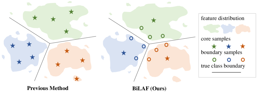
Figure 1: Design philosophy of our BiLAF framework. In contrast to previous methods, our method ensures the selection of central samples to maintain diversity while also reserving capacity to choose boundary samples to enhance decision boundary learning.

To fill in the research gap, the Active Finetuning task has been formulated in xie2023active, which focuses on the selection of samples for supervised finetuning using pretrained models. This method optimizes sample selection by minimizing the distributional gap between the selected subset and the entire data pool. Despite its notable performance, it fundamentally focuses on the diversity of samples, which overlooks the crucial aspect of uncertainty in data selection. Particularly, as the volume of data increases, the selected samples become increasingly redundant, thereby limiting the model’s capabilities, which is corroborated by the empirical experiments.

To address its shortcomings, we propose an innovative Bi-Level Active Finetuning Framework (BiLAF), designed to ensure that the sample selection process effectively balances both diversity and uncertainty, as shown in Fig. 1. The primary challenge lies in measuring uncertainty within the pretraining-finetuning paradigm. Traditional strategies, such as relying on classification confidence, are inapplicable in this scenario due to the lack of iterative training based on class labels. Alternatively, our focus shifts to the model’s decision boundary, a concept that has extensive theoretical lei2023understanding and methodological research burges1998tutorial; cao2019learning across various domains. Intriguingly, the global feature space of pretrained models can represent the interrelations between samples from different classes, allowing to find those support samples close to the decision boundary.

To elaborate, our BiLAF framework operates in two distinct stages. The first stage, Core Samples Selection, is dedicated to selecting central samples of each class. The selection method can be any that optimizes center samples, such as K-Means or ActiveFT xie2023active. The second stage, Boundary Samples Selection, involves our novel unsupervised denoising method to pinpoint outliers. Following this, we systematically select boundary samples around each center, using our specially developed boundary score, while avoiding redundancy by excluding similar samples.

Our contributions are summarized as follows:

• We propose a Bi-Level Active Finetuning Framework (BiLAF) emphasizing boundary importance to balance sample diversity and uncertainty.

• We innovate an unsupervised denoising method to eliminate the outlier samples and an iterative strategy to efficiently identifying boundary samples in feature space.

• Extensive experiments and ablation studies demonstrate the effectiveness of our method. Compared to current state-of-the-art approach, our method achieves a remarkable improvement of nearly 3% on CIFAR100 and approximately 1% on ImageNet.

2 Related Work

2.1 Active Learning / Finetuning

Active learning strives to maximize the utility of a limited annotation budget by selecting the most valuable data samples. In most pool-based scenarios, existing algorithms typically employ criteria of uncertainty or diversity for sample selection. Uncertainty-based methods typically make choices based on the difficulty of each sample, which is measured by various heuristics such as posterior probability lewis1994heterogeneous; wang2016cost, entropy joshi2009multi; luo2013latent, loss function huang2021semi; yoo2019learning, or the influence on the model performance freytag2014selecting; liu2021influence. In contrast, diversity-based algorithm selects representative data samples to approximate the distribution of the original data pool. The diversity can be quantified by the distance between the global sener2017active and local agarwal2020contextual; xie2023towards representations or other metrics like gradient directions ash2019deep or adversarial loss kim2021task; sinha2019variational.

However, the algorithms mentioned above are primarily designed for from-scratch training and face challenges within the pretraining-finetuning paradigm hacohen2022active; xie2023active. In response, ActiveFT xie2023active has been specifically developed for this context. It selects data by bringing the distribution of selected samples close to the original unlabeled pool in the feature space. ActiveFT tends to favor high-density areas in its selection, often overlooking boundary samples. In contrast, our proposed algorithm incorporates both diversity and uncertainty into the selection process, which is important for determining the decision boundary in the supervised finetuning.

2.2 Decision Boundaries in Neural Networks.

Decision boundaries are crucial in neural network-based classification models, significantly influencing performance and interpretability lei2023understanding; li2023support. Their optimization can greatly enhance model generalizability and accuracy, particularly in complex, high-dimensional data spaces xu2019locally; cao2019learning. In Support Vector Machines (SVMs), the decision boundary is fundamental to separating hyperplanes, and maximizing the geometric margin around this boundary is key for robust classification burges1998tutorial. This concept is also applicable to neural networks, where similar margin maximization can improve generalization. In the context of imbalanced datasets, adjusting the decision boundary is essential for the accurate classification of minority classes. Techniques like Label-Distribution-Aware Margin (LDAM) loss cao2019learning and Enlarged Large Margin (ELM) loss kato2023enlarged have been developed to modify the decision boundary, thus balancing generalization errors across classes. It has been observed that neural networks typically rely on the most discriminative or simplest features to construct decision boundaries ortiz2020hold; shah2020pitfalls. A theoretical framework for assessing decision boundary complexity through the novel metric of decision boundary (DB) variability, and its inverse relationship with generalizability, is presented in lei2023understanding.

However, in the field of active finetuning, the selection of Decision Boundaries has not yet been a focus of attention, although features from the pretrained model can provide an accurate representation of the sample boundary relationships. For the first time in the active finetuning task, we introduce a focus on Boundary Sample analysis.

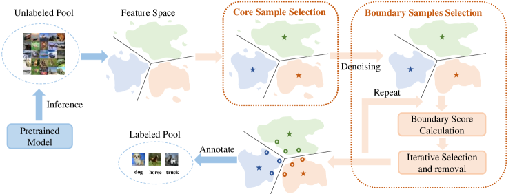
Figure 2: Our BiLAF framework in the Active Finetuning task. Within the high-dimensional feature space, the first stage core sample selection is dedicated to identifying pseudo-class centers. Building upon this, we have developed a denoising method to filter out noise samples. Subsequently, we compute the Boundary Score metric for each sample, which aids in the iterative selection of samples and the removal of candidates from the pool. Ultimately, the selected samples are labeled for supervised finetuning.

3 BiLAF: Bi-Level Active Finetuning

In this section, we introduce our novel Bi-Level Active Finetuning Framework (BiLAF), as illustrated in Fig. 2. BiLAF operates in two distinct stages: Initially, the Core Samples Selection stage is employed (Sec. 3.2). We identify multiple pseudo-class centers, intentionally selecting a slightly larger number of centers than the actual number of classes to ensure extensive coverage across all classes and to account for multiple centers within individual classes. The second stage involves our Boundary Samples Selection method (Sec. 3.3), which focuses on accurately identifying boundary samples for each class. Algorithm 1 summarizes the complete workflow of BiLAF.

3.1 Preliminary: Active Finetuning Task

The active finetuning task is formulated in xie2023active. Apart from a large unlabeled data pool $\mathcal{P}^{u}=\{\mathbf{x}_{i}\}_{i\in[N]}$ where $[N]=\{1,2,\dots,N\}$ same in the traditional active learning task, we have the access to a deep neural network model $f(\cdot;w_{0})$ with the pretrained weight $w_{0}$. It should be noted that the function $f(\cdot;w_{0})$ can be pretrained either on the current data pool $\mathcal{P}^{u}$ or any other data sources. Using the pretrained model, we can map the data sample $\mathbf{x}_{i}$ to the high dimensional feature space as $\mathbf{f}_{i}=f(\mathbf{x}_{i};w_{0})\in\mathbb{R}^{d}$, where $\mathbf{f}_{i}$ is the normalized feature of $\mathbf{x}_{i}$. Therefore, we can derive the feature pool $\mathcal{F}^{u}=\{\mathbf{f}_{i}\}_{i\in[N]}$ from $\mathcal{P}^{u}$.

Our task is to select the subset $\mathcal{P}^{u}_{\mathcal{S}}$ from $\mathcal{P}^{u}$ for annotation and the following supervised finetuning. $\mathcal{S}=\{s_{j}\in[N]\}_{j\in[B]}$ is a sampling strategy so that $\mathcal{P}_{\mathcal{S}}^{u}=\{\mathbf{x}_{s_{j}}\}_{j\in[B]}$, where $B$ is the annotation budget for supervised finetuning. The model would have access to the labels $\{\mathbf{y}_{s_{j}}\}_{j\in[B]}\subset\mathcal{Y}$ of this subset through the oracle, obtaining a labeled data pool $\mathcal{P}^{l}_{\mathcal{S}}=\{\mathbf{x}_{s_{j}},\mathbf{y}_{s_{j}}\}_{j\in[B]}$, where $\mathcal{Y}$ is the label space. Then, the pretrained model $f(\cdot;w_{0})$ is finetuned on $\mathcal{P}^{l}_{\mathcal{S}}$ supervisedly. Our objective is to choose the optimal sampling strategy to select the labeled set under the given budget to minimize the expectation error of the finetuned model.

3.2 Core Samples Selection

Core Samples Selection is a fundamental approach in active learning, aimed at identifying key samples that represent the entire dataset. Popular techniques include K-Means, Coreset sener2017active, and ActiveFT xie2023active, which primarily differ in their target designs and optimization processes. Within this framework, we adopt ActiveFT xie2023active, the most advanced model to date, as our primary method for the initial phase. For specific details on implementation of ActiveFT, please refer to Appendix LABEL:app:app_active. We utilize ActiveFT to obtain $K$ core samples, serving as pseudo-class centers, where $K$ is the predefined budget for central samples.

Then, we proceed with the boundary sample selection based on these $K$ pseudo-class centers.

3.3 Boundary Samples Selection

Decision boundaries are critical in classification problems, particularly in Active Finetuning. Selecting boundary samples for each class effectively can greatly enhance the training of the model’s decision boundaries, even within a limited budget, thus improving overall performance.

By leveraging pretrained models, data samples can be mapped to robust feature representations, which effectively elucidates the relationships between each sample, its intra-class counterparts, and inter-class samples from diverse classes. We design an innovative method for boundary sample selection for the first time in this task. Given the pseudo-class centers, our method comprises three steps: 1) Identifying the samples that belong to each pseudo-class center. 2) Implementing denoising processes on these samples. 3) Developing metrics to precisely select boundary points for each pseudo-class.

3.3.1 Step1: Clustering Process

Given $K$ pseudo-class centers denoted by $C=\{c_{1},c_{2},\ldots,c_{K}\}$ where $c_{i}\in[N]$, for the sample $\mathbf{x}_{j}$ with its corresponding feature $\mathbf{f}_{j}\in\mathbb{R}^{d}$, it is assigned to the pseudo-class center $c_{i}$ that minimizes the distance $D(\mathbf{f}_{j},\mathbf{f}_{c_{i}})$, which can be represented as:

$$c_{i}=\arg\min_{c\in C}D(\mathbf{f}_{j},\mathbf{f}_{c})$$ (1)

where $D(\cdot,\cdot)$ is the distance function. The choice of $D$ can be any distance metric, depending on the clustering design of the center selection model, which inherently assign each sample point to a corresponding pseudo-class center during optimization. Therefore, The Euclidean distance is used in our implementation.

3.3.2 Step2: Denoising process.

Boundary samples within a pseudo-class provide critical insights for optimizing the decision boundary. However, they can also introduce noise, potentially hindering the model’s performance. For each class $i$ containing $N_{i}$ samples, we set a removal ratio $P_{rm}$ to identify and eliminate $N_{i,rm}=N_{i}\cdot P_{rm}$ peripheral noisy samples from the candidate boundary set. This elimination is based on the sample density in the feature space, where we define the density distance as follows.

Definition 1 (Density Distance).

The density distance of a point is defined as the average distance to its $k$ nearest neighbors. Formally, for a given sample $x_{j}$ with the feature $\mathbf{f}_{j}$, its density distance $\rho({\mathbf{x}_{j}})$ is defined as:

$$\rho(\mathbf{x}_{j})=\frac{1}{k}\sum_{l=1}^{k}D(\mathbf{f}_{j},\mathbf{f}_{n_{jl}})$$ (2)

where $n_{jl}$ is the $l$-th nearest neighbor index of the sample $x_{j}$ in the feature space and $D$ is a distance function.

We get inspiration from the classical clustering method DBSCAN ester1996density to propose an Iterative Density-based Clustering (IDC) algorithm. IDC clusters the candidate points $\mathbf{X}_{i}=\{\mathbf{x}_{a_{i,1}},\mathbf{x}_{a_{i,2}},...\mathbf{x}_{a_{i,N_{i}}}\}$ where $a_{i,j}\in[N]$, beginning with the core sample index as the initialization set $U_{i}=\{c_{i}\}$. In the following each iteration, a fraction $P_{in}$ of points will be included, which means $N_{i,in}=N_{i}\cdot P_{in}$ peripheral samples are absorbed into the existing cluster $U_{i}$.

The density distance of each candidate point is redefined from Eq. 2 as the average distance to the nearest $k$ selected points which are in $U_{i}$. Formally, the density distance $\rho(\mathbf{x}_{j})$ for each remaining point $\mathbf{x}_{j}$ is calculated as:

$$\rho(\mathbf{x}_{j})=\frac{1}{k}\sum_{l=1,{n_{jl}}\in U_{i}}^{k}D(\mathbf{f}_{j},\mathbf{f}_{n_{jl}})$$ (3)

where $n_{jl}$ is the nearest $l$-th sample index of $\mathbf{x}_{j}$ which has been already included in the cluster. The $N_{i,in}$ densest samples with lowest density distance are chosen in each iteration. The process repeats until all points are selected. The order of inclusion into the class indicates the point’s proximity to the center, with points added later more likely to be noisy. Therefore, we can remove the last $N_{i,rm}$ samples.

Algorithm 1 Pseudo-code for BiLAF

Input: Unlabeled data pool $\mathcal{P}^{u}=\{\mathbf{x}_{i}\}_{i\in[N]}$, pretrained model $f(\cdot;w_{0})$, annotation budget $B$.
Parameter: Core samples budget $K$, removal ratio $P_{rm}$, density neighbours $k$, IDC cluster ratio $P_{in}$, opponent penalty coefficient $\delta$, distance function $D(\cdot,\cdot)$.
Output: The selected samples index $\mathcal{S}=\{s_{j}\}_{j\in[B]}$

1:$\triangleright$ Stage 1: Core Samples Selection

2:for $i\in[N]$ do

3:     $\mathbf{f}_{i}=f(\mathbf{x}_{i};w_{0})$

4:Select $K$ centers in feature space $\mathcal{F}$ using ActiveFT

5:$\triangleright$ Can be K-Means and any other core selection method

6:$\triangleright$ Stage 2: Boundary Samples Selection

7:for each pseudo-class $c_{i}$ do

8:$\quad\triangleright$ Step1: Assign the pseudo-class samples

9:     Initial the candidate index set $U^{0}_{i}=\{\}$

10:     for $j\in[N]$ do

11:         if $c_{i}==\arg\min_{c\in C}D(\mathbf{f}_{j},\mathbf{f}_{c})$ then

12:              Add the index $j$ to the set $U^{0}_{i}$               

13:$\quad\triangleright$ Step2: Iterative Density-based cluster then denoise

14:     Initialize the pseudo-class cluster $U_{i}=\{c_{i}\}$.

15:     while $|U^{0}_{i}|>|U_{i}|$ do

16:         for each candidate index $j\in U^{0}_{i}$ and $j\notin U_{i}$ do

17:              $\rho(\mathbf{x}_{j})=\frac{1}{k}\sum_{l=1,\mathbf{n_{jl}}\in U_{i}}^{k}D(\mathbf{f}_{j},\mathbf{f}_{n_{jl}})$ where

18:$\quad\quad\quad\quad\quad\quad n_{jl}$ is the nearest $l$-th sample index of $\mathbf{x}_{j}$.          

19:         Sort samples by increasing density distance $\rho(\mathbf{x}_{j})$

20:         Add the previous $P_{in}\cdot|U^{0}_{i}|$ samples to $U_{i}$      

21:     Remove the last $P_{rm}\cdot|U_{i}|$ samples from $U_{i}$ to denoise

22:$\quad\triangleright$ Step3: Selection Process

23:     Initialize opponent penalty counts $t_{l}=0$ for $l\neq i$

24:     for $m=1$ to $B_{i}$ do

25:         for each candidate index $j\in U_{i}$ do

26:              $d_{intra}(\mathbf{x}_{j})=\frac{1}{|U_{i}|}\sum_{l\in U_{i}}D(\mathbf{f}_{j},\mathbf{f}_{l})$

27:              $BS(\mathbf{x}_{j})=\min_{c_{l}\in C}^{i\neq l}\frac{\delta^{t_{l}}\cdot D(\mathbf{f}_{j},\mathbf{f}_{c_{l}})-d_{intra}(\mathbf{x}_{j})}{\max(D(\mathbf{f}_{j},\mathbf{f}_{c_{l}}),d_{intra}(\mathbf{x}_{j}))}$          

28:         Select $\mathbf{x}_{j_{min}}$ with the lowest Boundary Score if

29:             $m>1$, otherwise set $j_{min}=c_{i}$.

30:         Add the index $j_{min}$ to selected samples set $\mathcal{S}$

31:         $t_{l}=t_{l}+1$ where nearest opponent class is $l$ if

32:             $m>1$.

33:         Remove the nearest $|U_{i}|/B_{i}$ samples of $\mathbf{x}_{j_{min}}$

34:             from $U_{i}$      

35:return the selected samples index $\mathcal{S}$