Inference for Heterogeneous Graphical Models using Doubly High-Dimensional Linear-Mixed Models

Abstract

Motivated by the problem of inferring the graph structure of functional connectivity networks from multi-level functional magnetic resonance imaging data, we develop a valid inference framework for high-dimensional graphical models that accounts for group-level heterogeneity. We introduce a neighborhood-based method to learn the graph structure and reframe the problem as that of inferring fixed effect parameters in a doubly high-dimensional linear mixed model. Specifically, we propose a LASSO-based estimator and a de-biased LASSO-based inference framework for the fixed effect parameters in the doubly high-dimensional linear mixed model, leveraging random matrix theory to deal with challenges induced by the identical fixed and random effect design matrices arising in our setting. Moreover, we introduce consistent estimators for the variance components to identify subject-specific edges in the inferred graph. To illustrate the generality of the proposed approach, we also adapt our method to account for serial correlation by learning heterogeneous graphs in the setting of a vector autoregressive model. We demonstrate the performance of the proposed framework using real data and benchmark simulation studies.

Keywords: high-dimensional random effect, heterogeneous network, neighborhood selection, functional connectivity network, de-biased LASSO inference

1 Introduction

Gaussian graphical models (GGMs) capture conditional dependence relations among a set of variables, $\{Y_{1},Y_{2},\dots,Y_{p}\}$ via a graph $G=(V,E)$ with node set $V=\{1,2,\dots,p\}$ and edge set $E\subset V\times V$. For a mean zero multivariate normal vector $Y=\{Y_{j}:j\in V\}$ with covariance matrix $\Sigma$, the conditional dependence structure, and correspondingly, the edge set $E$, can be characterized by the nonzero entries of the inverse covariance matrix $\Omega=\Sigma^{-1}$. Specifically, two random variables $Y_{j}$ and $Y_{k}$ are conditionally independent if and only if $\Omega_{j,k}=0$. The value of $\Omega_{j,k}$ can be viewed as the weight of the edge $(j,k)$. Therefore, the problem of inferring the graph structure is effectively an (inverse-)covariance selection problem and has been extensively studied in high-dimensional settings, with applications in neuroscience Ng et al. (2013); Monti et al. (2017) and genomics Krumsiek et al. (2011); Zhao and Duan (2019), among other fields. Two of the most popular approaches for independent observations are the graphical lasso Yuan and Lin (2007); Friedman et al. (2008) and neighborhood selection Meinshausen and Bühlmann (2006). Other graph structure learning methods include greedy search Ray et al. (2015); Bresler (2015), structured regularization Cai et al. (2011); Defazio and Caetano (2012) and regularized score matching Lin et al. (2016). Recent developments in high-dimensional graphical modeling have also considered non-Gaussian observations Liu et al. (2012); Voorman et al. (2014); Yu et al. (2019) and functional data Solea and Li (2020); Qiao et al. (2019).

Estimates of graphical models provide valuable information about the strength of connectivity among variables. However, the uncertainty in these estimates needs to be quantified in order to answer scientific questions of interest — for instance, in brain functional connectivity studies, whether the estimated non-zero dependency between two brain regions indicates a real connection, or if the observed difference in the brain connectivity structures between two patient groups indicates a true population-level difference (Shojaie, 2020). As a result, inference for graphical models has received increasing attention in recent years. Examples include multiple testing with asymptotic control of false discovery rates Liu (2013), and direct testing of edge weights based on the asymptotic normality of different (de-biased) $\ell_{1}$-regularized estimators Janková and van de Geer (2017); Ren et al. (2015). See Janková and van de Geer (2018) for a detailed review.

This paper is motivated by the problem of inferring the graph structure of functional connectivity networks from multi-level functional magnetic resonance imaging (fMRI) data Smith et al. (2011). A prime example is the resting-state fMRI data from the Human Connectome Project (HCP); one of HCP’s main goals is to characterize the functional neural connections in healthy individuals Van Essen et al. (2013), and reliable inference for such connections is paramount to understanding the brain physiology Sporns (2007). Figure 1 illustrates our application setting: For each subject (i.e., level) $i=1,\ldots,n$, resting-state whole-brain fMRI signals give an indirect measure of the neuronal activation levels at multiple brain locations over time. Standard pre-processing leads to spatially distributed maps that define a set of brain regions $V=\{j:j\in 1,\ldots,p\}$, with details to be described in Section 6. Each brain region has an associated fMRI signal describing its activation pattern over time, denoted by $Y^{i}_{j}$. Without loss of generality, we center the observations for each brain region, $Y^{i}_{j}$, at zero.

Learning the functional connectivity graph structure from ${Y^{i}_{j}}$ presents two primary challenges: (i) fMRI observations over time for a single brain node typically exhibit serial correlation; and (ii) the data have a clustered or multi-level structure, where each cluster, or level, corresponds to the observations of a specific subject. While the serial correlation can be mitigated through various whitening procedures including model-based pre-whitening procedures Olszowy et al. (2019); Woolrich et al. (2001) or simple down-sampling approaches, the complications due to the clustered structure of the data have not been extensively studied in this setting. Many neuroscience studies ignore the heterogeneity inherent in multi-level data and simply infer a single graphical model for all subjects Dyrba et al. (2020). This assumes a fixed dependence structure for all the subjects, which is contrary to a growing body of evidence that points to considerable subject-level heterogeneity in functional connectivity networks Monti et al. (2017); Mumford and Nichols (2006). Such heterogeneity cannot be easily addressed with resampling techniques e.g., Narayan and Allen (2016), which lack theoretical guarantees for type-I error control and are computationally demanding when the number of brain regions is large. Another popular approach is to employ a two-stage strategy: in the first stage, separate graphical models are inferred for each subject; in the second stage, individual-level summary statistics are used for group-level analysis Narayan and Allen (2016); Deshpande et al. (2009); Morgan et al. (2011). P-value aggregation via Fisher’s method Deshpande et al. (2009) and t-test based on individual-level statistics Morgan et al. (2011) are two typical examples. While straightforward, such methods ignore any shared brain network information across subjects, which can lead to inefficient estimation and inference. More importantly, they can lead to conflicting conclusions from different second-stage aggregation choices, as well as erroneous conclusions due to not properly accounting for the uncertainty in first-stage estimates Chiang et al. (2017). We illustrate the limitations of these two-stage approaches through a simple toy example depicted in Figure 1. In the toy example, we infer the connectivity between a given node and six other nodes using the neighborhood selection approach from a marginal model perspective (see Figure 1 for details). Specifically, as shown in Table 1, the fixed GGM method that ignores the heterogeneity can result in false discoveries, even when the population-level average network is of interest. Two-stage approaches may lead to conflicting conclusions, and may result in both inflated type-I errors and/or reduced power.

The analysis of resting-state fMRI signals introduces additional challenges to brain network inference. In contrast to task-based fMRI data, where a shared task pattern enables the alignment of observations across subjects, resting-state fMRI data lacks a clear correspondence between time points across subjects. This absence of alignment renders methods such as functional graphical model approaches Solea and Li (2020); Qiao et al. (2019) impractical, as these methods rely on the assumption of aligned underlying signals or functions. Therefore, to bridge the gap in existing approaches for inferring population-level brain connectivity networks while accounting for subject-level heterogeneity, in Section 2 we propose a mixed effect Gaussian graphical model. Utilizing a neighborhood-based estimation strategy similar to Narayan and Allen (2016), for each edge, the proposed approach models the subject-level coefficients as random realizations centered around a population mean. The key difference is the estimation and inference approach: we recast the resulting model as a doubly high-dimensional linear mixed model, where the number of fixed and random effects parameters can be larger than the sample size. In addition to the doubly high-dimensional structure, the fixed and random design matrices in the corresponding linear mixed models also have considerable overlap. These factors significantly complicate the theoretical analysis, rendering existing approaches inadequate. We overcome these challenges by utilizing penalized estimation and inference strategies, as well as tools from random matrix theory. We obtain consistent estimators and establish a valid inference framework for the corresponding parameters in Section 3. We also provide consistent estimation of the mixed effect variance components in Section 4.1 and demonstrate the performance of the proposed approach via extensive simulations in Section 5 and analysis of HCP fMRI data in Section 6.

The model proposed in Section 2 naturally accounts for the heterogeneity in individual-level connectomes. However, heterogeneity also arises in many other applications, including data harmonization Yu et al. (2018) and integration of multiple batches of genomic data Zhang et al. (2020). The proposed estimation and inference framework for doubly high-dimensional linear mixed models can also be utilized in such problems. Moreover, while in this paper we focus on estimation of undirected GGMs using data without serial correlation within each level, we show in Section 4.2 that our proposed method can be extended to inferring graphs based on a first-order Vector Autoregressive (VAR) model, and is thus able to account for (weak) serial correlations.

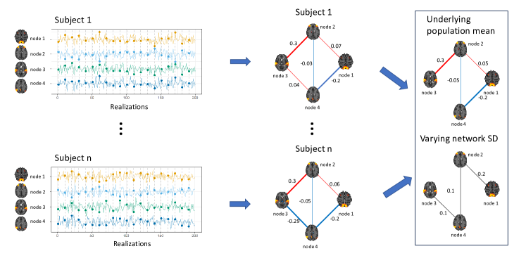
Figure 1: Illustration of the proposed functional connectivity brain network analysis. Left panel: fMRI signals measuring the activation level at each brain node for individual subjects. Middle panel: Subject-level brain networks inferred from the associated fMRI data. The lines between the brain nodes depict connectivity, with the numbers denoting the connectivity strength, red lines representing positive connectivity, and blue lines representing negative connectivity. Right panel: The output of our proposed model. This is the underlying population-level brain network and the associated network of standard deviations (SD) summarizing inter-subject variation around the population-level brain network.

	Edge
	1—2	1—3	1—4	1—5	1—6	1—7
fixed effect coefficients $\beta$	0.50	-0.40	0.20	0.40	0.00	0.00
SD of random effect coefficients	1.50	0.00	0.50	0.75	0.00	0.50
Approach	Power				Type-I error
Two-stage t-test	0.255	0.795	0.165	0.460	0.050	0.040
Two-stage Fisher’s method	1.000	0.380	0.660	0.925	0.075	0.500
Fixed GGM	0.750	0.755	0.310	0.605	0.035	0.150
Mixed effect GGM	0.285	0.980	0.240	0.505	0.025	0.055

Table 1: Toy example where we infer the group-level conditional dependence using a neighborhood selection approach, and target the connection between node 1 and the rest of the six nodes. We infer using two-stage approaches, the fixed GGM approach and the mixed effect GGM approach. We generate data from a marginal model following model (2), where the fixed effect coefficients and the standard deviation (SD) of the corresponding random effect coefficients are shown in the top table. The noise terms independently and identically follow the standard normal distribution. For each of the 20 subjects, we simulate 10 observations. We then use the neighborhood selection approach to infer the network edges. For the fixed GGM approach, we concatenate observations from all subjects and fit a single GGM using a simple linear regression model. For two-stage approaches, we use simple linear regression in the first stage for each subject, then in the second stage use either Fisher’s method to aggregate p-values Deshpande et al. (2009) or use t-test on each subject’s coefficient estimates Morgan et al. (2011). For the mixed effect GGM approach, we use a linear mixed-effect model with each subject as a cluster (see Section 2 for model details). Power/Type-I errors are computed based on 500 replications. The simulations show that when there is high subject-level heterogeneity, two-stage approaches may have highly-inflated type-I error (Fisher’s method for edge 1—7), or have lower power to detect dependence (t-test method) compared to the mixed effect GGM approach. The fixed GGM approach shows an inflated type-I error for edge 1—7.

2 Method

2.1 Notations

We denote an $m\times m$ identity matrix by $I_{m}$. For a matrix $A$, we denote by $A_{j,k}$ the $(j,k)$ entry of $A$, by $A_{j}$ the $j$th column of $A$, and by $A_{-j}$ the sub-matrix of $A$ obtained by dropping the $j$th column. Similarly, we use index sets $S$, $\{j,k\}$ and $1:j$ to denote multiple columns/entries in a matrix/vector, and use $-S$, $-\{j,k\}$ and $-\{1:j\}$ to denote a sub-matrix/sub-vector obtained by removing the indicated columns/entries. We denote by $\|A\|_{2}$ the matrix norm of $A$, which is the maximum singular value of $A$. The Frobenius norm of $A$ is denoted by $\|A\|_{F}$, which is equal to $\sqrt{\mathop{\mathrm{tr}}(AA^{\top})}$ with $\mathop{\mathrm{tr}}(A)$ denoting the trace of $A$. We use $\sigma(A)$, $\sigma_{\min}(A)$ and $\sigma_{\max}(A)$ to represent the singular values, the minimum singular value, and the maximum singular value of $A$. For a set of values $\{u_{l}\}_{l=1}^{K}$ and a set of matrices $\{A_{l}\}_{l=1}^{K}$, we let $\mathop{\mathrm{diag}}\left(\{u_{l}\}_{l=1}^{K}\right)$ be the diagonal matrix with $(l,l)$ entry $u_{l}$, and let $\mathop{\mathrm{diag}}\left(\{A_{l}\}_{l=1}^{K}\right)$ be the block-diagonal matrix with the $l$th block $A_{l}$.

A random variable $U$ is sub-Gaussian with parameter $u$ if $\forall\ t\in\mathop{\mathbb{R}}$, $\mathop{\mathbb{E}}\left(e^{tU}\right)\leq\exp(ut^{2}/2)$. We define $\mathop{\mathrm{SG}}(u)$ as the class of all sub-Gaussian random variables with mean 0 and parameter $u$. A random vector $V$ is sub-Gaussian with parameter $v$ if for any vector $x$ with $\|x\|_{2}=1$, we have $x^{\top}V\in\mathop{\mathrm{SG}}(v)$. We denote the class of such sub-Gaussian random vectors by $\mathop{\mathrm{SGV}}(v)$.

For two scalars $a$ and $b$, we write $a\asymp b$ if $c_{1}|b|\leq|a|\leq c_{2}|b|$ for some positive constants $c_{1}$, $c_{2}$. We write $a\vee b=\max(a,b)$, and $a\wedge b=\min(a,b)$. We use $a=O(b)$ to indicate that $a\leq c_{1}b$ for some constant $c_{1}>0$, and use $a=o(b)$ to mean that $a/b\xrightarrow{}0$. Throughout the paper, we use $c,\ c_{0},\ c_{1},\ldots$ to represent positive constants, whose values may vary from line to line.

2.2 Problem Setup

Suppose that for each subject $i=1,\dots,n$ the observed data matrix, $Y^{i}\in\mathop{\mathbb{R}}^{m\times p}$, includes $m$ observations for each of the $p$ nodes. Without loss of generality, we assume the observations for each node are centered at zero. The assumption of equal number of observations per subject is made for simplicity and our results continue to hold if the $i$th subject has $m_{i}$ observations, as long as $c_{1}\max_{i}(m_{i})\leq\min_{i}(m_{i})\leq c_{2}\max_{i}(m_{i})$ for some constants $c_{1},c_{2}>0$. The population-level connectivity network is characterized by the inverse covariance matrix $\Omega$, and subject-specific conditional independent networks are denoted by $\Omega^{i}$.

We would like to infer the edges in the population-level network, while accounting for subject-level heterogeneity. To this end, we propose a neighborhood-based method where we model the subject-specific edge weight $\Omega^{i}_{j,k}$ as random variables centered at the population-level edge weight $\Omega_{j,k}$. Specifically, we assume the following neighborhood-based model for a node $j\in V$:

$$Y^{i}_{j}=\sum_{k=1,k\neq j}^{p}Y^{i}_{k}b^{i}_{j,k}+\epsilon^{i}_{j},\quad i=1,\dots,n,$$ (1)

where given $Y^{i}_{k},k\neq j$, the subject-level connectivity coefficients, $b^{i}_{j,k}$, have mean $b_{j,k}$ and variance $\sigma^{2}_{j,k}$. The coefficients $b^{i}_{j,k}$ and their mean $b_{j,k}$ are proportional to the true edge weights $\Omega^{i}_{j,k}$ and $\Omega_{j,k}$, respectively. The randomness in $b^{i}_{j,k}$ captures the subject-level heterogeneity, while its mean $b_{j,k}$ captures the shared dependence structure across subjects. Our main goal is to test whether a pair of nodes $(j,k)$ are functionally connected at a population level, i.e., $H_{0}:b_{j,k}=0$.

The model in equation (1) can be seen as a linear mixed model (LMM), formulated as:

$$Y^{i}_{j}=Y^{i}_{-j}\beta_{j}+Y^{i}_{-j}\gamma^{i}_{j}+\epsilon^{i}_{j},\quad i=1,\dots,n.$$ (2)

Here, we treat node $j$ as the outcome variable and the associated vectors $Y^{i}_{j}\in\mathop{\mathbb{R}}^{m}$ as the outcome vector of observations. We treat the rest of the $p-1$ nodes as covariates. The matrix $Y^{i}_{-j}\in\mathop{\mathbb{R}}^{m\times(p-1)}$ serves as both the fixed and random effect design matrices. The fixed effect coefficients $\beta_{j}\in\mathop{\mathbb{R}}^{p-1}$ correspond to $\left\{b_{j,k}\right\}_{k=1,k\neq j}^{p}$, which represent the (scaled) edge weights $\Omega_{j,-j}$. The random effect coefficients $\gamma^{i}_{j}=\left\{b^{i}_{j,k}-b_{j,k}\right\}_{k=1,k\neq j}^{p}$ represent the subject-level variation of these $p-1$ (scaled) weights. The hypothesis $H_{0}:\ b_{j,k}=0$ is thus equivalent to $H_{0}^{\prime}:\ \beta_{j,k}=0$, allowing us to recast the graphical selection problem as that of estimating and inferring the fixed effect coefficients in an LMM. Since the number of brain nodes $p$ is typically large in brain connectivity studies, the resulting LMM is doubly high-dimensional, i.e., both fixed and random effects are high-dimensional.

Despite its increasing relevance in applications, rigorous estimation and inference procedures for doubly high-dimensional LMMs are lacking. Methods for LMMs with high-dimensional fixed effects and low-dimensional random effects Lin et al. (2020); Bradic et al. (2020) are not readily extendable to this setting. In addition, while Expectation-Maximization has been proposed for estimation Monti et al. (2017), the consistency of the resulting estimator has not been thoroughly examined. Likewise, while consistent, valid inference for the estimator of Li et al. (2018) has not been explored. Most related to our setting is the recent work by Li, Cai and Li Li et al. (2021), denoted LCL hereafter. The work of LCL proposes a de-biased LASSO-based inference framework for doubly high-dimensional linear mixed models; however, as common in the LMM literature, it assumes a form of independence between the fixed and random effect design matrices—the fixed effect design matrix is assumed to have zero mean conditional on the random effect design matrix. This restrictive assumption constitutes a key shortcoming in our graphical modeling application, where the fixed and random effect design matrices are identical, leading to a violation of the zero conditional mean assumption by LCL. This assumption can also be restrictive in many other applications, whenever the fixed effects and the random effects share a non-empty set of covariates Li et al. (2018). Moreover, the LCL framework requires the number of random effects to be no larger than the number of observations per subject, which further limits its applicability.

Motivated by the neighborhood-based model in (1), in this paper, we develop a new estimation and inference framework for doubly high-dimensional LMMs in (2). To this end, we propose a penalized estimation and inference framework for the fixed effect coefficients. We make two key extensions to the work of Li et al. (2021) that enable valid inference of heterogeneous GGMs: (i) our approach accommodates a larger number of random effects than the number of observations per subject; and (ii) it does not require conditional independence and only imposes minimal assumptions on the relationship between the fixed and the random effects. Through these extensions, our model provides the first mixed-model inference framework for learning functional connectivity networks in multi-level settings.

2.3 The Proposed Approach

To achieve consistent estimation for the doubly high-dimensional LMM in equation (2), we assume the true $\beta_{j}^{*}$ coefficients are sparse, with support $S_{j}$ and cardinality $s_{j}=|S_{j}|\ll p$. Let $\Sigma^{i}$ be the $p\times p$ subject-specific covariance matrix for subject $i$. Throughout this paper, we assume that, conditional on the covariance matrices $\Sigma^{i}$, the matrices $Y^{i}$ are independent and follow a matrix normal distribution $Y^{i}\mid\Sigma^{i}\sim\mathrm{MN}_{m\times p}(0,I_{m},\Sigma^{i})$, for $i=1,\dots,n$. This implies that within-subject observations are independent conditional on the subject-specific covariance matrix. To allow for subject-level heterogeneity, we assume the subject-specific covariance matrices $\Sigma^{i}$ are random, and we denote by $\Sigma$ the corresponding population-level covariance matrix. Conditional on the matrix $Y^{i}_{-j}$, the random effect coefficients $\gamma^{i}_{j}$ and the noise vectors $\epsilon^{i}_{j}$ are independent with mean zero and covariance $\Psi_{j}\in\mathop{\mathbb{R}}^{(p-1)\times(p-1)}$ and $R^{i}_{j}\in\mathop{\mathbb{R}}^{m\times m}$, respectively. We assume $\gamma^{i}_{j}\in\mathop{\mathrm{SG}}(c_{1}\|\Psi_{j}\|_{2})$ and $\epsilon^{i}_{j}\in\mathop{\mathrm{SG}}(c_{2}\|R^{i}_{j}\|_{2})$, which implies that $Y^{i}_{j}-Y^{i}_{-j}\beta_{j}|Y^{i}_{-j}\in\mathop{\mathrm{SG}}(c_{1}\|\Psi_{j}\|_{2}+c_{2}\|R^{i}_{j}\|_{2})$.

Similar to other specifications of graphical models (see, e.g., Voorman et al., 2014; Chen et al., 2015), the model in equation (2) specifies the conditional distribution of $Y_{j}$ as a function of other variables, $Y_{-j}$. In this model, the population-level network edge $(j,k)$ is characterized by the $\beta_{j,k}$ coefficient, such that $(j,k)\in E$ if and only if $\beta_{j,k}\neq 0$, providing a convenient specification of the conditional dependence structure while accounting for subject-level variability of the edges. In this work, we focus on developing an inference framework for the model in equation (2) and leave the characterization of joint probability distributions that are consistent with the conditionally-specified models Wang and Ip (2008) to future research. We let $p$ grow with the sample size $n$ and the number of observations per subject $m$. In the main text, we focus on the setting where $p>c_{0}m$ for some constant $c_{0}>1$, which is most relevant to our application, and defer the case of $p<c_{0}m$ for some constant $0<c_{0}<1$ to the Appendix.

The unknown random effect covariance matrices $\Psi_{j}$ pose challenges to the estimation and inference of the fixed effect coefficients $\beta_{j}$. Following the quasi-likelihood approach in Fan and Li (2012), we use proxy matrices in place of the unknown covariance matrix. Specifically, we use the proxy matrix $\Sigma_{a}^{i,(j)}=aY_{-j}^{i}(Y_{-j}^{i})^{\top}+I_{m}$, with a fixed positive constant $a$, to approximate the covariance matrix of $Y^{i}_{j}$, which is $\Sigma^{i,(j)}_{\theta}=Y_{-j}^{i}\Psi_{j}(Y^{i}_{-j})^{\top}+R^{i}_{j}$, for $i=1,\dots,n$. We then use a LASSO estimator for the fixed effect coefficients $\beta_{j}$ that leverages the proxy matrix $\Sigma_{a}^{i,(j)}$ to “decorrelate” the observations. In addition, we propose an inference framework based on the de-biased LASSO method. As we will discuss later, our estimation and inference procedures for the coefficients $\beta_{j}$ do not depend on the estimates of the variance components $\Psi_{j}$ and $R_{j}^{i}$ and are, hence, well-defined.

2.3.1 LASSO estimator for $\beta_{j}$

We propose a LASSO estimator for the fixed effect coefficients $\beta_{j}$ based on the de-correlated observations. To this end, let $\Sigma_{a}^{(j)}=\mathop{\mathrm{diag}}\left(\{\Sigma_{a}^{i,(j)}\}_{i=1}^{n}\right)$, and $Y$ be the $nm\times p$ matrix obtained by vertically stacking $\{Y^{i}\}_{i=1}^{n}$. Our proposed estimator $\hat{\beta}_{j}$ is given by

$$\hat{\beta}_{j}=\operatorname*{\arg\!\min}_{\beta_{j}\in\mathbb{R}^{p-1}}\frac{1}{2\mathop{\mathrm{tr}}\left((\Sigma_{a}^{(j)})^{-1}\right)}\left\|(\Sigma_{a}^{(j)})^{-1/2}(Y_{j}-Y_{-j}\beta_{j})\right\|_{2}^{2}+\lambda_{a,j}\|\beta_{j}\|_{1},$$ (3)

with tuning parameter $\lambda_{a,j}>0$. In Section 3, we show that under mild assumptions $\hat{\beta}_{j}$ is a consistent estimator of $\beta_{j}$, for a suitable choice of $\lambda_{a,j}$ and for any choice of constant $a$.

Taking $\Sigma_{a}^{(j)}=I_{nm}$ in (3) leads to the classical LASSO estimator. While it is easy to show that this estimator is also consistent, it is known that due to the correlation across observations, this misspecified estimator has sub-optimal rate of convergence Li et al. (2021).

2.3.2 Inference based on de-biased LASSO

We next propose an inference framework for the coefficient $\beta_{j,k}$, $k\in V\backslash\{j\}$ based on the asymptotic normality of the de-biased LASSO estimator. The de-biasing procedure builds on the idea in Zhang and Zhang (2014), which uses regularized regression to estimate the bias term of the LASSO estimator.

For $k\in V\backslash\{j\}$, our de-biased estimator $\hat{\beta}_{j,k}^{(\mathrm{db})}$ is defined as

$$\hat{\beta}_{j,k}^{(\mathrm{db})}=\hat{\beta}_{j,k}+\frac{\sum_{i=1}^{n}\left(\hat{w}^{i}_{j,k}\right)^{\top}\left(\Sigma_{b}^{i,(j,k)}\right)^{-1/2}\left(Y_{j}^{i}-Y^{i}_{-j}\hat{\beta}_{j}\right)}{\sum_{i=1}^{n}\left(\hat{w}^{i}_{j,k}\right)^{\top}\left(\Sigma_{b}^{i,(j,k)}\right)^{-1/2}Y^{i}_{j}},$$ (4)

where the proxy covariance matrices $\Sigma_{b}^{i,(j,k)}$ are defined as

$$\Sigma_{b}^{i,(j,k)}=aY^{i}_{-\{j,k\}}(Y^{i}_{-\{j,k\}})^{\top}+I_{m},\quad\Sigma_{b}^{(j,k)}=\mathop{\mathrm{diag}}\left(\{\Sigma_{b}^{i,(j,k)}\}_{i=1}^{n}\right),$$

with the same constant $a$ used in $\Sigma_{a}^{(j)}$; and the projection related terms $\hat{\kappa}_{j,k}$, $\hat{w}^{i}_{j,k}$ are defined as

$$\hat{\kappa}_{j,k}=\operatorname*{\arg\!\min}_{\kappa_{j,k}\in\mathbb{R}^{p-2}}\frac{1}{2\mathop{\mathrm{tr}}\left(\left(\Sigma_{b}^{(j,k)}\right)^{-1}\right)}\left\|\left(\Sigma_{b}^{(j,k)}\right)^{-1/2}\left(Y_{k}-Y_{-\{j,k\}}\kappa_{j,k}\right)\right\|_{2}^{2}+\lambda_{j,k}\|\kappa_{j,k}\|_{1}$$

$$\hat{w}^{i}_{j,k}=\left(\Sigma_{b}^{(j,k)}\right)^{-1/2}\left(Y_{k}-Y_{-\{j,k\}}\hat{\kappa}_{j,k}\right),$$

with tuning parameter $\lambda_{j,k}>0$.

Here, the vector $\hat{w}^{i}_{j}$ is approximately the orthogonal complement of the projection of the vector $\left(\Sigma_{b}^{(j,k)}\right)^{-1/2}Y_{j}$ onto the space spanned by the columns of $\left(\Sigma_{b}^{(j,k)}\right)^{-1/2}Y_{-j}$, where the projection vector $\hat{\kappa}_{j,k}$ is computed via LASSO regression. We use the proxy matrix $\Sigma_{b}^{(j,k)}$ to “decorrelate” observations $Y_{k}$ and $Y_{-\{j,k\}}$ in the LASSO regression. Note that we define the proxy matrix $\Sigma_{b}^{(j,k)}$ differently from LCL Li et al. (2021). This modification is crucial to successfully establishing the asymptotic normality of the de-biased estimator $\hat{\beta}_{j,k}^{(\mathrm{db})}$, especially in the setting where the fixed effect design matrix has overlapping columns with the random effect design matrix.

Denoting by $z_{\alpha}$ the $\alpha$th quantile of a standard normal distribution, we can construct a two-sided $(1-\alpha)\times 100$% confidence interval for the coefficient $\beta_{j,k}$ as $\hat{\beta}_{j,k}^{(\mathrm{db})}\pm z_{\alpha/2}\sqrt{\hat{V}_{j,k}}$, where $\hat{V}_{j,k}$ is a sandwich-type estimator of the variance of $\hat{\beta}^{(\mathrm{db})}_{j}$, defined as:

$$\hat{V}_{j,k}=\frac{\sum_{i=1}^{n}\left|(\hat{w}_{j,k}^{i})^{\top}\left(\Sigma_{b}^{i,(j,k)}\right)^{-1/2}\left(Y_{j}^{i}-Y_{-j}^{i}\hat{\beta}_{j}\right)\right|^{2}}{\left|\sum_{i=1}^{n}(\hat{w}_{j,k}^{i})^{\top}\left(\Sigma_{b}^{i,(j,k)}\right)^{-1/2}Y_{j}^{i}\right|^{2}}.$$ (5)

3 Theoretical Analysis

In this section, we show that, under mild conditions, the proposed LASSO estimator $\hat{\beta}_{j}$ in (3) is consistent, and the proposed de-biased LASSO estimator $\hat{\beta}^{(\mathrm{db})}_{j,k}$ in (4) is asymptotically normal. We first state the assumptions under which we establish the consistency of $\hat{\beta}_{j}$ defined in (3). Recall that we use $c,c_{0},c_{1},\dots$ to denote generic positive constants whose values may vary line by line.

Assumption 1.

2. The number of observations per subject $m$ and the number of covariates $p$ satisfy $p>c_{0}m$ for some constant $c_{0}>1$, and $p>c_{1}$ for some suitably large constant $c_{1}>0$. Moreover, $p\log(p)/(mn)=o(1)$.

3. $\forall\ i,j$, $\sigma(\Sigma)\asymp\sigma(R^{i}_{j})\asymp\|\Psi_{j}\|_{2}\asymp 1$, and $\|\Sigma^{i}-\Sigma\|_{2}\leq\sigma_{\min}(\Sigma)-c_{2}$ for some constant $c_{2}>0$.

In Assumption 1.1, we restrict the growth rate of $p$ relative to $m$ and $n$. Moreover, we assume $p/m$ is no smaller than a positive constant $c_{0}>1$, which is the situation most relevant to our application. In the Appendix, we discuss the case when $p/m\leq 1/c_{0}$ for some constant $c_{0}>1$.

By Weyl’s theorem, Assumption 1.2 implies $\sigma(\Sigma^{i})\asymp 1$ for all $i=1,\dots,n$ Bhatia (2007), requiring the singular values of the covariance matrices $\Sigma$, $\Sigma^{i}$, and $R^{i}_{j}$ to be both lower and upper bounded by positive constants. Note that we do not require independent and identically distributed noise terms for each observation. Consequently, our model is applicable across various settings, including those involving time series outcomes. Specifically, it accommodates scenarios where the noise terms conform to an autoregressive model of order 1, since the covariance matrices $R^{i}_{j}$ in such cases are Kac-Murdock-Szego matrices with all eigenvalues of order $O(1)$ Trench (1999).

To establish the consistency of $\hat{\beta}_{j}$, we only require an upper bound on the singular values of the covariance matrices $\Psi_{j}$ in Assumption 1.2. However, later we also require one of the following assumptions on $\Psi_{j}$ to hold in order to establish the asymptotic normality of the de-biased estimator; we state these assumptions here for convenience.

Assumption 2.

2. (Diagonal structure): $\forall\ j$, $\Psi_{j}=\mathop{\mathrm{diag}}(\psi_{j})$ for a vector $\psi_{j}\in\mathop{\mathbb{R}}^{p-1}$. The support of $\psi_{j}$ is $S_{\psi_{j}}$ with cardinality $s_{\psi_{j}}<c_{1}m\wedge n$ for some constant $c_{1}>0$. Moreover, $\min(\psi_{S_{\psi_{j}}})\asymp\max(\psi_{S_{\psi_{j}}})\asymp 1$.

3. (Bounded eigenvalues): $\forall\ j$, $\sigma_{\min}(\Psi_{j})\asymp 1$.

Assumption 2.1 allows us to cover the settings when the minimum singular values of the covariance matrices $\Psi_{j}$ are not bounded away from zero. In such a case, we consider a sparse diagonal structure for the matrices $\Psi_{j}$, under which our results hold with slightly different sample size assumptions.

The next result establishes the theoretical properties of the proposed estimator $\hat{\beta}_{j}$ in (3).

Theorem 1 (Fixed effect estimator consistency).

Suppose Assumption 1.1 and Assumption 1.2 hold and that $\lambda_{a,j}=c_{1}\sqrt{p\log(p)/(nm)}$ for a suitably large $c_{1}>0$. Then, with probability at least $1-4\exp\{-cn\}-12\exp\{-c\log(n)\}-3\exp\{-cmnp^{-1}\}$,

$$\left\|\hat{\beta}_{j}-\beta_{j}^{*}\right\|_{\delta}=O_{p}\left(s_{j}^{1/\delta}\sqrt{\frac{p\log(p)}{mn}}\right),\quad\delta\in\{1,2\},$$

$$\left\|(\Sigma_{a}^{(j)})^{-1/2}Y(\hat{\beta}_{j}-\beta_{j}^{*})\right\|_{2}^{2}=O_{p}\left(s_{j}\log(p)\right).$$

If, in addition, Assumption 2.1 holds, taking $\lambda_{a,j}=c_{2}\sqrt{\log(p)\log^{2}(n)/n}$ for a suitably large $c_{2}>0$, we have with probability at least $1-4\exp\{-cn\}-12\exp\{-c\log(n)\}-3\exp\{-cmnp^{-1}\}$ that

$$\left\|\hat{\beta}_{j}-\beta_{j}^{*}\right\|_{\delta}=O_{p}\left(s_{j}^{1/\delta}\sqrt{\frac{\log^{2}(n)\log(p)}{n}}\right),\quad\delta\in\{1,2\},$$

$$\|(\Sigma_{a}^{(j)})^{-1/2}Y(\hat{\beta}_{j}-\beta_{j}^{*})\|_{2}^{2}=O_{p}\left(\frac{s_{j}m\log^{2}(n)\log(p)}{p}\right).$$

Theorem 1 shows that the de-correlated LASSO estimator $\hat{\beta}_{j}$ achieves $\ell_{1}$, $\ell_{2}$ and prediction consistency. The proof of Theorem 1 is based on the classical proof of the consistency of the LASSO estimator in regression settings Bühlmann and Van De Geer (2011) with multiple key modifications to extend it to our setting. One crucial step is to show that the restricted eigenvalue condition Bühlmann and Van De Geer (2011) holds for the matrix product $X\left(aZZ^{\top}+I\right)^{-1}X^{\top}$, where $X$ is the fixed effect design matrix and $Z$ is the random effect design matrix. Since in our setting the fixed and random effect design matrices are identical, we cannot rely on techniques such as those adopted in Li et al. (2021) where the conditional mean independence assumption between $X$ and $Z$ is used to remove the dependence on the matrix $Z$. Instead, we jointly study the contribution of both the fixed and random effect design matrices, and use results from random matrix theory Tropp (2015) to directly characterize the eigenvalue distribution of the relevant quantities. In particular, we obtain a set of tight bounds for functions of the non-zero singular values of the matrices $Y^{i}$ under Assumption 1. This key result, which may be of independent interest, is presented in Lemma 7 in Appendix B. We state the other lemmas necessary to prove Theorem 1 in Appendix B.

Next, we state a simplified version of the assumptions under which we establish the asymptotic normality of the de-biased LASSO estimator $\hat{\beta}^{(\mathrm{db})}_{j,k}$ defined in (4). In order to allow for such a simplification, we have made some additional mild assumptions such as $\sigma\left(G^{(j)}_{k}\right)\asymp p$ under Assumption 2.2, $c_{1}\leq\sigma_{\min}\left(G^{(j)}_{k}\right)\leq\sigma_{\max}\left(G^{(j)}_{k}\right)\leq c_{2}m$ under Assumption 2.1, and $|H_{k}^{(j)}|\asymp s_{j}\asymp 1$. Recall that model (2) implies that given $Y^{i}_{-j}$, the vector $Y^{i}_{j}-Y^{i}_{-j}\beta_{j}$ is sub-Gaussian with covariance matrix $\Sigma_{\theta}^{i,(j)}=Y^{i}_{-j}\Psi_{j}(Y^{i}_{-j})^{\top}+R^{i}_{j}$. If we were to assume that given $Y^{i}_{-\{j,k\}}$, the covariance matrix of $Y^{i}_{k}$ has a “sandwich” form akin to $\Sigma_{\theta}^{i,(j)}$, namely $G_{k}^{(j)}=Y^{i}_{-\{j,k\}}\Psi_{j,k}(Y^{i}_{-\{j,k\}})^{\top}+R^{i}_{j,k}$ for some matrix $\Psi_{j,k}\in\mathop{\mathbb{R}}^{(p-2)\times(p-2)}$ and $R^{i}_{j,k}\in\mathop{\mathbb{R}}^{m\times m}$, we could then characterize the rates of $\|G_{k}^{(j)}\|_{2}$ and $\sigma_{\min}\left(G_{k}^{(j)}\right)$ with the above assumed rates (see Lemma 10).

Assumption 3.

2. $\forall\ j,k$, conditioning on the matrix $Y^{i}_{-\{j,k\}}$, the vector $Y^{i}_{k}-Y^{i}_{-\{j,k\}}\kappa_{k}^{(j),*}$ has mean zero and variance $G^{(j)}_{k}$, and belongs to the class $\mathop{\mathrm{SGV}}(c_{1}\|G^{(j)}_{k}\|_{2})$. The support of $\kappa_{k}^{(j),*}$, $H^{(j)}_{k}$, has cardinality $|H^{(j)}_{k}|$ satisfying $\|\kappa_{k}^{(j),*}\|_{1}\leq c_{1}|H^{(j)}_{k}|$.

3. If Assumption 2.1 holds, then $p^{2}\log(p)\ll nm^{3}$, $m\log^{7}(n)\ll n$, $\log(n)\log(p)\ll n$. If Assumption 2.2 holds, then $p\log(n)\log(p)\leq c_{3}mn$.

In Assumption 3.1, we specify an upper bound for $\|\kappa_{k}^{(j),*}\|_{1}$. This is not too restrictive, because given that the variance of each node is bounded (implied by Assumption 1.2), it is reasonable to expect that the coefficients $\kappa_{k}^{(j),*}$ are not too large in absolute value. In the case of no subject-level heterogeneity, that is $Y^{i}\sim\mathrm{N}(0,\Sigma)$ and $\kappa_{k}^{(j),*}=\left(\Sigma_{-\{j,k\},-\{j,k\}}\right)^{-1}\Sigma_{-\{j,k\},k}$, it is easy to show that $\sum_{l=1,l\neq k}^{p-1}\left|(\kappa_{k}^{(j),*})_{l}\sqrt{(\Omega_{j})_{k,k}}/\sqrt{(\Omega_{j})_{l,l}}\right|\leq|H_{k}^{(j)}|$, and $\|\kappa_{k}^{(j),*}\|_{1}\leq c_{1}|H_{k}^{(j)}|$ is satisfied.

In Assumption 3.1, we also specify the conditional distribution of $Y^{i}_{k}$ given $Y^{i}_{-\{j,k\}}$. We do not assume a specific structure for the covariance matrix $G_{k}^{(j)}$, but only require mild bounds on the minimum and maximum eigenvalues (Appendix C).

Assumption 3 indicates different sample size requirements according to different structures of $\Psi_{j}$ in Assumption 2. Note that Assumption 2 can be relaxed at the cost of stricter sample size requirements: if we only assume $\|\Psi_{j}\|_{2}\leq c_{1}$ and drop Assumption 2, the asymptotic normality property of $\hat{\beta}^{(\mathrm{db})}_{j,k}$ will hold with some additional sample size assumptions (Appendix C.1, Remark 13), which would restrict the growth rate of $p$ to be slower than $n$.

The next result establishes the asymptotic normality of the estimator $\hat{\beta}^{(\mathrm{db})}_{j,k}$ in (4).

Theorem 2.

Under Assumptions 1 and 3, we have with probability at least $1-c_{1}\exp\{-cn\}-c_{2}\exp\{-c\log(n)\}-c_{3}\exp\{-cmn/p\}-c_{4}\exp\{-c\log(p)\}-c_{5}\exp\{-cmn\}$, $\left(V_{j,k}\right)^{-1/2}\left(\hat{\beta}_{j,k}^{(\mathrm{db})}-\beta_{j,k}^{*}\right)=R_{j,k}+o_{p}(1)$, where $R_{j,k}\xrightarrow[]{d}\mathrm{N}(0,1)$ and the variance $V_{j,k}$ is given by

$$V_{j,k}=\frac{\sum_{i=1}^{n}(\hat{w}_{j,k}^{i})^{\top}\left(\Sigma_{b}^{i,(j)}\right)^{-1/2}\Sigma^{i,(j)}_{\theta}\left(\Sigma_{b}^{i,(j)}\right)^{-1/2}\hat{w}^{i}_{j,k}}{\left|\sum_{i=1}^{n}(\hat{w}_{j,k}^{i})^{\top}\left(\Sigma_{b}^{i,(j)}\right)^{-1/2}Y_{j}\right|^{2}}.$$

The proof of Theorem 2 builds on the properties of the projection vectors $\hat{\kappa}_{j,k}$ and the orthogonal complement of the projection $\hat{w}^{i}_{j,k}$. Specifically, we show that $\left(V_{j,k}\right)^{-1/2}\left(\hat{\beta}_{j,k}^{(\mathrm{db})}-\beta_{j,k}^{*}\right)$ can be divided into two terms, where one term is $o_{p}(1)$ and the other term can be shown to be asymptotically normal, thanks to the Lyapunov central limit theorem. As in the proof of Theorem 1, we extensively use the core Lemma 7 to bound quantities involving both the fixed effect and the random effect design matrices.

A novel feature of our results, compared to those in the literature, including LCL Li et al. (2021), is that we establish the unconditional asymptotic normality of $\hat{\beta}^{(\mathrm{db})}_{j,k}$. In contrast, other approaches establish the asymptotic normality only conditionally on the random effect design matrices, even when the design matrices are assumed to be random. This unconditional normality is crucial for our application to brain connectivity network inference, and to the best of our knowledge, this is the first attempt to characterize the unconditional asymptotic properties of the fixed effect coefficients estimator with random design matrices in high-dimensional LMMs.

The lemmas required to prove Theorem 2 are presented in Appendix C. Lemma 12 gathers several intermediate results necessary to prove Theorem 2.

Finally, we show that the sandwich estimator $\hat{V}_{j,k}$, defined in (5), is a consistent estimator of $V_{j,k}$ under Assumption 4. We apply the same simplifications as we did for Assumption 3.

Assumption 4.

2. If Assumption 2.1 holds, then $m^{2}\log^{5}(n)\log^{2}(p)\ll n$.

3. If Assumption 2.2, then $\log^{2}(p)\log^{4}(n)\ll n$.

Theorem 3.

Under Assumptions 1, 3, and 4, with probability at least $1-c_{1}\exp\{-cn\}-c_{2}\exp\{-c\log(n)\}-c_{3}\exp\{-cmn/p\}-c_{4}\exp\{-c\log(p)\}-c_{5}\exp\{-cmn\}$ we have $\hat{V}_{j,k}/V_{j,k}=1+o_{p}(1).$

4 Extensions

4.1 Variance Component Estimation

An appealing property of the proposed estimation and inference framework for the fixed effects is that we do not need to estimate the variance components $\theta=(\Psi,\{R^{i}\}_{i=1}^{n})$. This is convenient when only the fixed effects are of interest. However, variance components also contain important information and should not be ignored. In our application of brain network analysis, a non-zero random effect variance component indicates the presence of subject-level heterogeneity in the connectivity between two brain nodes. In other applications, such as heritability analysis Sofer (2017) and genome-wide association studies (Aulchenko et al., 2007), the variance component estimates are necessary for downstream analysis, or may be of independent interest.

Unfortunately, estimating the variance components in doubly high-dimensional LMM settings introduces unique challenges that have not been addressed by existing approaches. In particular, the method of (Li et al., 2018) assumes bounded $m$, in order to use a Cholesky decomposition for estimating the random effect covariance matrix. The sample-splitting approach of (Li et al., 2021) requires $m>q$ for $q$ random effect covariates, which restricts its applicability in high dimensions. We extend the sample-splitting approach to doubly high-dimensional LMM settings, and propose a penalized moment-based estimator for selecting and estimating the variance components. In particular, we allow for $m$ to be smaller than $q$ and to grow with $n$. To simplify the problem, in the following, we assume that the noise terms are independent and identically distributed within each subject’s observations, i.e., $R^{i}=\sigma_{e}^{2}I_{m}$. Moreover, we assume $\Psi$ is a diagonal matrix satisfying Assumption 2.1, such that $\Psi=\mathop{\mathrm{diag}}(\psi)$. To simplify the notation and to broaden the scope of the framework, we will present the proposed estimators and the theoretical results under a more general LMM formulation:

$$y^{i}=X^{i}\beta+Z^{i}\gamma_{i}+\epsilon_{i},\quad i=1,\dots,n,$$ (6)

where each $y^{i}\in\mathop{\mathbb{R}}^{m}$ is the observation vector, $X^{i}\in\mathop{\mathbb{R}}^{m\times p}$ and $Z^{i}\in\mathop{\mathbb{R}}^{m\times q}$ are the design matrices with $X^{i}\mid\Sigma_{X}^{i}\sim\mathrm{MN}_{m\times p}(0,I_{m},\Sigma_{X}^{i})$ and $Z^{i}\mid\Sigma_{Z}^{i}\sim\mathrm{MN}_{m\times q}(0,I_{m},\Sigma_{Z}^{i})$. Conditional on $X^{i}$, the random effect coefficients $\gamma_{i}\in\mathop{\mathbb{R}}^{q}$ and the noise term $\epsilon_{i}\in\mathop{\mathbb{R}}^{m}$ are independent with variance $\Psi$ and $R^{i}$, and satisfy $\gamma_{i}\in\mathop{\mathrm{SGV}}(c_{1}\|\Psi\|_{2})$, $\epsilon_{i}\in\mathop{\mathrm{SGV}}(c_{2}\|R^{i}\|_{2})$, respectively. The fixed effect coefficient vector $\beta$ has support $S$ with cardinality $s$. See the Appendix for additional details on the model definition.

It is known that the variance components become non-identifiable if the random effect covariance matrix is proportional to the noise covariance Wang (2013). In our case, this would happen if $Z^{i}\Psi(Z^{i})^{\top}=c\sigma_{e}^{2}I_{m}$, for some constant $c>0$. However, given that we assume the diagonal of $\Psi$ is sparse, we have $\sigma_{\min}\left(Z^{i}\Psi(Z^{i})^{\top}\right)=0$ whereas $\sigma_{\min}(\sigma_{e}^{2}I_{m})=\sigma_{e}^{2}>0$, ensuring identifiability.

Let $\theta=(\psi,\sigma_{e}^{2})$ denote the variance components. To estimate $\theta$, we adopt a sample-splitting approach, and partition the $n$ subjects into three sub-samples of similar sizes with index set $S_{k}$, $k=1,2,3$, such that $n_{k}=|S_{k}|$ and $n_{1}\asymp n_{2}\asymp n_{3}$. We start by using the first $n_{1}$ subjects to estimate the fixed effect parameters $\beta$, denoting the estimates as $\hat{\beta}$. We then use the second sub-sample with $n_{2}$ subjects to estimate the vector $\psi$. Denoting $\hat{r}_{i}=y^{i}-X^{i}\hat{\beta}$, $i\in S_{2}$, we define the penalized moment-based estimator for $\psi$ with tuning parameter $\lambda_{\theta}$, as:

$$\hat{\psi} =\operatorname*{\arg\!\min}_{\psi\in\mathop{\mathbb{R}}^{q}}\sum_{i\in S_{2}}\left\|\hat{r}_{i}\hat{r}_{i}^{\top}-\mathop{\mathrm{diag}}(\hat{r}_{i})\mathop{\mathrm{diag}}(\hat{r}_{i})-Z^{i}\mathop{\mathrm{diag}}(\psi)(Z^{i})^{\top}+\sum_{l=1}^{q}\psi_{l}\mathop{\mathrm{diag}}(Z_{l}^{i})\mathop{\mathrm{diag}}(Z_{l}^{i})\right\|_{F}^{2}$$

$$\quad+\lambda_{\theta}\|\psi\|_{1}.$$ (7)

The estimator for $\psi$ is constructed from the second moment of the residuals $r_{i}=y^{i}-X^{i}\beta^{*}$ by noticing that $\mathbb{E}\left(\left(r_{i}r_{i}^{\top}\right)_{l,k}\right)=\left(Z^{i}\Psi(Z^{i})^{\top}\right)_{l,k}$. In the high-dimensional setting here considered, we adopt a LASSO regularization to guarantee the consistency of the estimator and simultaneously perform variable selection.

Finally, we use the third sub-sample with $n_{3}$ subjects to estimate the noise variance $\sigma_{e}^{2}$. To this end, we propose a simple moment-based estimator defined as

$$\hat{\sigma}_{e}^{2}=\frac{1}{n_{3}m}\sum_{i\in S_{3}}\mathop{\mathrm{tr}}\left(\hat{r}_{i}\hat{r}_{i}^{\top}-Z^{i}\mathop{\mathrm{diag}}(\hat{\psi})(Z^{i})^{\top}\right),$$ (8)

where $\hat{r}_{i}$ is computed based on the the first $n_{1}$ samples, and $\hat{\psi}$ is computed based on the second $n_{2}$ samples.

We gather the assumptions needed to prove the consistency of the proposed variance component estimator $(\hat{\psi},\hat{\sigma}_{e}^{2})$ in Assumption 5 below. The true values are denoted by $\theta^{*}=(\psi^{*},\sigma_{e}^{2,*})$.

Assumption 5.

2. The vectors $\gamma_{i}$ and $\epsilon_{i}$ are normally distributed with mean zero and variance matrices $\Psi$, $\sigma_{e}^{2}I_{m}$, respectively. The covariance matrix $\Psi$ satisfies Assumption 2.1.

3. Letting $s_{Z}=\max_{i}\max_{j}\sum_{k=1,k\neq j}^{q}\bm{1}\left\{(\Sigma_{Z}^{i})_{j,k}\gg\log(nq^{2})/\sqrt{m}\right\}$, we have $\sqrt{m}\gg\log(nq)$, $nm\gg\max\left\{q^{3/2}\log(q)\log^{2}(n),\log(q)\log(n)\log(nq^{2})\left(s_{Z}\sqrt{m}+q\log(nq^{2})\right)\right\}$, $nm^{3}\gg q^{2}\log(q)\log^{2}(n)$.

4. $\sqrt{n}m^{2}\gg ss_{\psi}q\log(p)\log(q)\log(n)\log(nmq)$.

Theorem 4.

Under Assumption 1 and 5.1–5.2, with probability at least $1-c_{1}\exp\{-c\log(nq)\}-c_{2}\exp\{-cn\}-c_{3}\exp\{-c\log(n)\}-c_{4}\exp\{-cmn/q\}-c_{5}\exp\{-c\log(q)\}$, we have

$$\|\hat{\psi}-\psi^{*}\|_{\delta} \leq s_{\psi}^{1/\delta}\frac{q\log(n)\log(p)\log(nmq)}{\sqrt{n}m},\quad\delta=1,2.$$

Theorem 5.

Under Assumption 1 and 5, we have $|\hat{\sigma}_{e}^{2}-\sigma_{e}^{2,*}|=o_{p}(1)$ with probability at least $1-c_{1}s_{\psi}q\log^{3}(n)/(nm)-c_{2}\exp\{-cnm\}-c_{3}\exp\{-cn\}-c_{4}\exp\{-c\log(n)\}-c_{5}\exp\{-cmn/q\}-c_{6}\exp\left\{-c{n^{2}m^{2}}/({sq^{2}\log^{4}(n)\log(p)})\right\}$.

Similar to the proof of Theorem 1, we leverage random matrix theory Tropp (2015) to bound the eigenvalues of matrix products and follow the classical proof of the consistency of the LASSO estimator Bühlmann and Van De Geer (2011). As previously mentioned, our estimator allows $q$ to be larger than $m$, and also applies to the case where $q$ is smaller than $m$ (Appendix E). The related lemmas are collected in Appendix E.

4.2 High-Dimensional Heterogeneous Vector Autoregressive Models

In this section, we show that the proposed estimation and inference framework can be also extended to heterogeneous high-dimensional first-order VAR models. Different from GGMs describing an unconditional functional connectivity brain network, VAR modeling has been a popular approach for inferring the joint effective connectivity network Friston (2011) among multiple brain regions Chen et al. (2011). Specifically, the VAR coefficients of the fitted model reveal Granger causal relations among brain regions Granger (1969); Shojaie and Fox (2022). A subject-specific first-order VAR model is formulated as

$$Y^{i}(t)=\Phi^{i}Y^{i}(t-1)+\epsilon^{i}(t),$$ (9)

for observations $\{Y^{i}(t)\}_{t=1}^{T}$, VAR coefficient matrix $\Phi^{i}$ and error term $\{\epsilon^{i}(t)\}_{t=1}^{T}$ for the $i$-th subject.

Recent developments have extended the VAR model to high-dimensional settings for stationary Shojaie and Michailidis (2010); Basu and Michailidis (2015); Han et al. (2015) and non-stationary Safikhani and Shojaie (2022) time series, and for nonlinear Zhang et al. (2022); Liu and Chen (2020), sub-Gaussian Zheng and Raskutti (2019) and non-Gaussian Tank et al. (2021) time series. However, these extensions are limited to modeling a single subject’s network. Two-stage approaches are often adopted by neuroscientists for inference in multi-subject settings: in the first stage, separate VAR models are fitted for each subject; in the second stage, individual-level summary statistics are used for group-level analysis Deshpande et al. (2009); Morgan et al. (2011); Narayan and Allen (2016). This includes aggregating each subject’s p-values for entries of $\Phi$ via Fisher’s method Deshpande et al. (2009), and conducting a two-sample t-test based on individual-level summary statistics Morgan et al. (2011). However, two-stage approaches have significant limitations. Firstly, they often fail to adequately address the uncertainty associated with estimated individual-level statistics in the second-stage analysis Chiang et al. (2017), which potentially results in inaccurate group-level conclusions. Secondly, subject-level analyses overlook shared structural information among individuals, leading to less efficient estimates for the group-level structure. Lastly, choosing different methodologies for the second stage can lead to different conclusions. These limitations can be problematic when making inferences in the presence of subject-level heterogeneity.

To overcome the above issues, mixed-effect VAR (MEVAR) models have been proposed for multi-subject brain signal analyses Gorrostieta et al. (2012, 2013). In MEVAR models, the VAR coefficients $\Phi^{i}$ in (9) are random variables centered at the population-level matrix $\Phi$ such that $\Phi^{i}=\Phi+\Gamma^{i}$, where the matrix $\Phi$ represents the population-level effective connectivity brain network. However, current applications of this model are limited to low-dimensional fMRI observations Gorrostieta et al. (2012, 2013); Brose et al. (2015); Wang et al. (2012). Even though there is an extensive body of work on incorporating mixed effects in VAR models, the majority focus on random coefficient AR models from a Bayesian perspective Liu and Tiao (1980); Nandram and Petruccelli (1997), while the rest are concerned with low-dimensional MEVAR models Nicholls and Quinn (1981); Vaněček (2008) (see Regis et al. (2022) for a detailed overview). Theoretical results on multivariate MEVAR models are rare Regis et al. (2022), and, to the best of our knowledge, valid frequentist inference for high-dimensional MEVAR models has not been investigated.

Our proposed doubly high-dimensional LMM framework can be adopted to infer the population structure $\Phi$ in a high-dimensional first-order MEVAR model. Let the vector $\mathop{\mathrm{vec}}(A)$ denote the vectorized matrix A through vertical stacking of its columns, and let $A\otimes B$ denote the Kronecker product between two matrices $A$ and $B$. We can rewrite the model in equation (9) as:

$$\tilde{Y}^{i}=\tilde{X}^{i}\mathop{\mathrm{vec}}(\Phi)+\tilde{X}^{i}\mathop{\mathrm{vec}}(\Gamma^{i})+\tilde{\epsilon}^{i},\quad i=1,\dots,n,$$ (10)

where

$$\tilde{Y}^{i}=\left(\begin{array}[]{c}Y^{i}(2)\\ \ldots\\ Y^{i}(T)\end{array}\right),\quad\tilde{X}^{i}=\left(\begin{array}[]{c}\left(Y^{i}(1)\right)^{\top}\otimes I_{p}\\ \ldots\\ \left(Y^{i}(T-1)\right)^{\top}\otimes I_{p}\end{array}\right),\quad\tilde{\epsilon}^{i}=\left(\begin{array}[]{c}\epsilon^{i}(2)\\ \ldots\\ \epsilon^{i}(T)\end{array}\right).$$

In equation (10), $\tilde{X}^{i}$ is the design matrix, $\mathop{\mathrm{vec}}(\Phi)$ is the fixed effect coefficient vector, and $\mathop{\mathrm{vec}}(\Gamma^{i})$ is the random effect coefficient vector. We can thus recast the problem of inferring $\Phi$ in a first-order MEVAR as the problem of inferring fixed effect coefficients in a doubly high-dimensional LMM, for which our proposed LMM framework applies. We can also show that inferring the whole matrix $\Phi$ is equivalent to inferring each row of $\Phi$ separately, which drastically accelerates computation.

We can show that the resulting penalized estimate for $\Phi$ is consistent, and the inference framework yields valid confidence intervals. Most of the proof follows the techniques used for the theoretical results in Section 3. However, due to the presence of correlated rows in the design matrix $\tilde{X}^{i}$, we introduce a pivotal lemma that extends the theoretical results in Section 3 to the case of a first-order MEVAR mode (Appendix G.2, Lemma 20). Using the properties of a stationary first-order VAR process, this lemma connects the singular values of $\tilde{X}^{i}$ to the singular values of a standard Gaussian matrix and facilitates the remainder of the proof.

We demonstrate through a simulation study in Appendix G.1 that our proposed framework works well for inferring the matrix $\Phi$ for high-dimensional first-order MEVAR models.

5 Simulation Studies

5.1 Simulation Setting

For ease of exposition, we generate data from a doubly high-dimensional LMM formulated as:

$$y^{i}=X^{i}\beta+X^{i}\gamma_{i}+\epsilon_{i},\quad i=1,\dots,n,$$ (11)

with $X^{i}\mid\Sigma_{X}^{i}\sim\mathrm{MN}_{m\times p}(0,I_{m},\Sigma_{X}^{i})$, $\gamma_{i}\sim\mathrm{N}(0,\mathop{\mathrm{diag}}(\psi))$ and $\epsilon_{i}\sim\mathrm{N}(0,\sigma_{e}^{2}I_{m})$. This is equivalent to analyzing the edges connected to one single node in a GGM.

We compare our approach with two competing approaches: (i) the LCL method of Li et al. (2021), and (ii) the de-biased LASSO method Zhang and Zhang (2014) (referred to as dblasso) as a benchmark approach which ignores the subject-level heterogeneity among observations. We compare the methods in terms of the total mean squared error (total MSE) for the estimates of all $\beta_{l}$ coefficients, the power of testing non-zero coefficients, the type-I error for testing zero coefficients at 5% significance level, and the coverage of 95% confidence intervals. We also compare the method proposed in Section 4.1 for estimation of the variance components, $\theta=(\psi,\sigma_{e}^{2})$, with the method of LCL by assessing the MSE of the noise variance $\sigma_{e}^{2}$, the total MSE for estimates of all $\psi_{l}$, and the selection consistency of the non-zero random effect variance components $\psi_{S_{\psi}}$. The selection consistency performance is evaluated via the Matthews correlation coefficient (MCC) Matthews (1975); MCC summarizes true positive and false positive rates, with higher values indicating more accurate identification of the non-zero variance components.

We generated data from the doubly high-dimensional linear mixed model specified in (11) with $n\in\{30,50,80,100\}$ and $m\in\{15,30,50,70\}$. For each combination of $(n,m)$, we set $p\in\{20,60\}$ and replicate 200 independent Monte Carlo simulations. We set $(\beta_{1}^{*},\beta^{*}_{2},\beta^{*}_{6},\beta^{*}_{7},\beta^{*}_{9})=(1,0.5,0.2,0.1,0.05)$ and $\beta^{*}_{l}=0$ for the remaining $l$’s. The random effects $\gamma_{i}$ and the noise terms $\epsilon_{i}$ were independent realizations of two multivariate normal distributions $\mathrm{N}(0,\mathop{\mathrm{diag}}(\psi))$ and $\mathrm{N}(0,\sigma_{e}^{2}I_{m})$, respectively. The true values of the variance components $(\psi^{*},\sigma_{e}^{2,*})$ are set as follows: $(\psi^{*}_{1},\psi^{*}_{4},\psi^{*}_{7},\psi^{*}_{9},\psi^{*}_{10},$ $\psi^{*}_{12},\psi^{*}_{16},\psi^{*}_{20})=(2,2,0.1,0.1,4,0.1,2,0.1)$, with the remaining $\psi^{*}_{l}$’s set to 0, and $\sigma_{e}^{2,*}=1$. The fixed effect design matrices $X^{i}$ were independent realizations of a matrix normal distribution $X^{i}\mid\Sigma_{X}^{i}\sim\mathrm{MN}_{m\times p}(0,I_{m},\Sigma_{X}^{i})$. To generate $\Sigma_{X}^{i}$, we first generated a population-level covariance matrix $\Sigma_{X}$, which was set as a sparse random matrix with diagonal entries $1$ and off-diagonal entries drawn independently from a mixture distribution: each entry was either set to zero with probability $0.8$, or was drawn from a uniform distribution $\mathrm{Unif}(-0.5,0.5)$. This choice was motivated by the nature of sparsely correlated brain networks. Each $\Sigma_{X}^{i}$ was then generated as a perturbed version of $\Sigma_{X}$ by (i) determining varying off-diagonal entries of $\Sigma_{X}^{i}$ by drawing a Bernoulli random variable with success probability 0.2; and (ii) generating variations by adding a mean zero normal perturbation with standard deviation 0.1. To ensure symmetry, only the entries in the upper-diagonal of $\Sigma_{X}^{i}$ were considered as candidates for perturbation. We repeated the above two steps if the generated $\Sigma_{X}^{i}$ was not positive definite. The resulting $\Sigma^{i}_{X}$ represent subject-level heterogeneity in the brain networks.

We used cross-validation with MSE as the error criteria to select the tuning parameters $\lambda_{a}$ for $\hat{\beta}$, $\lambda_{j}$’s for $\hat{\kappa}_{j}$ and $\lambda_{\theta}$ for variance components. We used the R function cv.glmnet from the R package glmnet (v4.1-3, (Friedman et al., 2010)) to implement the cross-validation algorithm. The constant $a$ in the proxy matrix is also viewed as a tuning parameter. We followed the approach described in Li et al. (2021) to select an optimum $a$ via cross-validation: for each candidate value of $a$, we let the algorithm select the values for the rest of the tuning parameters, and used cross-validation based on MSE to select an optimal $a$. We present the results based on the optimal $a$. We used the authors’ publicly available R code for LCL Li et al. (2021), and used the hdi R-package Dezeure et al. (2015b) for dblasso.

5.2 Simulation Results

Results for inference on fixed effect parameters $\beta$ are summarized in Figure 2. The proposed method controls the type-I error rate at the nominal level, whereas LCL and dblasso show inflated type-I errors in various settings (Figure 2a, 2b): when the random effect variance is large ($\psi_{10}=4$ for $\beta_{10}$), tests by dblasso have type-I errors as high as 0.74; LCL’s type-I error reaches 0.28 when the random effect variance is zero (for $\beta_{11}$); both methods show higher type-I errors with increasing $m$. Results for $p=60$ are presented in Appendix F.1 Table 2. When $p=60$, the type-I error of LCL improves for small $m$, but is still as high as 0.23 for large $m$ values; dblasso has high type-I error regardless of $p$, which is not surprising. Interestingly, dblasso often fails when testing covariates with non-zero random effect variances, and LCL often fails when testing covariates with zero random effect variances, especially when $m$ is large.

The confidence intervals constructed by the proposed method provide good coverage, while those constructed by LCL and dblasso show poor coverage in some settings (Figure 2c, 2d). The pattern of the confidence interval coverage is similar to the pattern of the type-I error: LCL has coverage lower than 0.81 for $\beta_{11}$ at $p=20$, $m=70$, and has insufficient coverage for covariates with zero random effect variance when $m$ is large (Appendix F.1 Table 3); dblasso’s coverage is always lower than 0.8 for some $\beta_{l}$’s (Figure 2c), and is as low as 0.24 for $p=60$ (Appendix F.1 Table 3); both methods have worse coverage with increasing $m$.

Since dblasso has poor confidence interval coverage and highly inflated type-I error, we do not include it in the power comparison for testing $\beta_{l}$’s. The proposed method in general has comparable power against LCL (Figure 2e, 2f and Appendix F.1 Table 4).

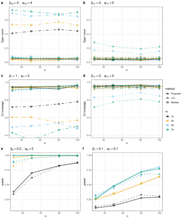
Figure 2: a,b: Type-I error for testing $\beta_{l}$’s at the 0.05 significance level (0.05 marked by red solid line), for the proposed method, LCL and dblasso. c,d: 95% confidence interval coverage (0.95 marked by red solid line) for fixed effect coefficients, for the proposed method, LCL and dblasso. e,f: Power for testing fixed effect coefficients at the 0.05 significance level, for the proposed method and LCL. All results are computed at $p=20$ based on 200 Monte Carlo simulations, and are plotted separately for each method, each $m$, and against increasing $n$. The title of each subplot shows the true values of the targeted fixed effect coefficient $\beta_{l}$, and the corresponding random effect variance component $\psi_{l}$.

In terms of estimating the fixed effect coefficients, the proposed method always has smaller total MSE than LCL (Figure 3a and Appendix F.1 Table 5). Fixed effect coefficient estimates by dblasso always have the smallest total MSE.

Since dblasso does not provide variance component estimates, it is not included for comparison in Figure 3. When $m<q$, LCL is not able to provide variance component estimates, while our method provides sensible estimates in all settings (Figure 3b, 3c). When $m>q$, our method’s estimate of $\sigma_{\epsilon}^{2}$ are not as good as LCL’s (Figure 3b), but its total MSEs for the random effect variance components are comparable with LCL (Figure 3c and Appendix F.1 Table 5).

We also examined the selection consistency of the random effect variance components evaluated by MCC. The proposed method selects the variance components much more accurately than LCL, and the accuracy improves with increasing $n$ and $m$ (Figure 3d). LCL has poor selection accuracy, and is less accurate with increasing $n$. Examining the proportion of simulations that yield non-zero estimates for each variance component reveals that LCL over selects zero variance components (Appendix F.1 Figure 7).

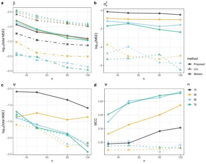
Figure 3: a: Total MSE on the $\log_{10}$ scale for estimating the fixed effect coefficients $\beta$, for the proposed method, LCL and dblasso. b: MSE on the $\log_{10}$ scale for estimating the noise variance $\sigma^{2}_{e}$, for the proposed method and LCL. c: Total MSE on the $\log_{10}$ scale for estimating the random effect variance components $\psi$, for the proposed method and LCL. d: Average MCC for identifying non-zero variance components for the proposed method and LCL, where we use non-zero estimates to select non-zero variance components. Values are computed at $p=20$ based on 200 Monte Carlo simulations, are plotted separately for each method, each $m$, and are against increasing $n$.

Finally, in terms of computational time, the proposed method is slightly slower than LCL for fixed effect estimation and inference, but is much faster for variance component estimation. The differences become more pronounced for large $p$ (Appendix F.1 Figure 6).

6 Data Application

We employ the proposed method to learn brain connectivity networks using the Human Connectome Project (HCP) resting-state fMRI data Van Essen et al. (2013). HCP has acquired high-quality functional and structural imaging data from healthy adult subjects in an effort to enhance the understanding of neural connectivity. Here, we focus on analyzing the resting-state fMRI data of 160 unrelated subjects, among which 80 are recreational drug users, and the rest are non-users. Each fMRI scan provides a signal with a temporal resolution of 0.73 seconds and a spatial resolution of 2-mm isotropic Smith et al. (2015). Standard pre-processing steps were applied to the fMRI signals Smith et al. (2013), including spatial normalization Glasser et al. (2013) and artifacts removal Griffanti et al. (2014); Smith et al. (2015). Then a Group Independent Component Analysis was applied to generate $200$ spatially-distributed brain nodes Smith et al. (2014). Using a dual-regression, $200$ associated time series of length $1,200$ were obtained, each one representing the activation pattern of a brain node over time (see Smith et al., 2015, for more details). To remove the temporal correlation, we down-sampled each time-series to one of length $120$, which we assume consists of independent observations.

We apply the proposed method to the user and the non-user groups separately, estimating and testing the significance of the functional connectivity (network edges) between every pair of brain nodes in each group, and estimating the variance component for each network edge. For the latter, we assume a sparse diagonal covariance matrix for the random effects and we split the samples into three equal-sized sub-samples for estimation. To account for the numerical asymmetry of the neighborhood selection approach, in each group we set the edge $E_{j,k}$ based on $\hat{\beta}_{j\leftrightarrow k}=(\hat{\beta}_{j,k}+\hat{\beta}_{k,j})/2$. The corresponding variance of $\hat{\beta}_{j\leftrightarrow k}$ is computed as $\hat{V}_{j\leftrightarrow k}=(\hat{V}_{j,k}+\hat{V}_{k,j})/2$. The p-value for testing the null hypothesis $H_{0}:\beta_{j\leftrightarrow k}=0$ is then computed based on these averaged quantities.

For comparison, we also apply the LCL, the dblasso methods and the two-stage approaches using t-test (two-stage t-test) or Fisher’s method (two-stage Fisher) to estimate and test the statistical significance of $\beta_{j\leftrightarrow k}$ for the non-user group. The dblasso approach ignores the within-subject correlations and subject-level variations, yielding network strength estimates that are equivalent to applying our model with $a=0$ in the proxy matrices $\Sigma_{a}^{(j)}$.

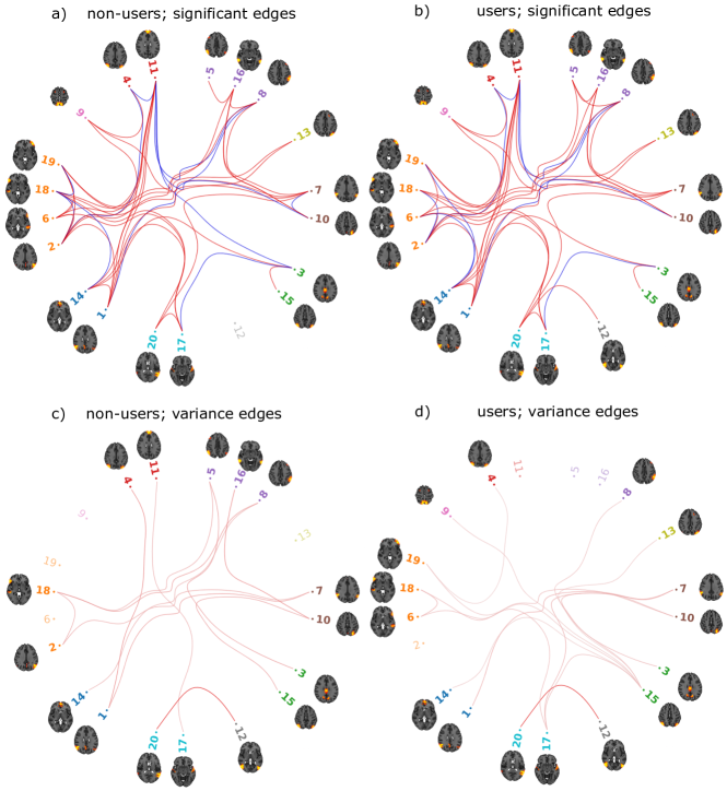
Figure 4: Estimated brain sub-networks, and associated variances, in recreational drug users and non-users as estimated by the proposed method. We present the results only for a subset of the 200 nodes that are associated with the default mode network, i.e., the brain regions that are active during passive rest. These were selected based on visual examination of the brain nodes. The node clusters in the networks are defined through hierarchical clustering based on the fixed effect estimates from the proposed method. a,b: The most significant edges (adjusted p-values $<1\times 10^{-13}$) in each group. Red edges represent positive edge strength, and blue edges represent negative edge strength. c,d: The edges in the top 25% based on their variances, selected from those depicted in sub-plots a and b. The edge width is proportional to the estimate of edge variance, with thicker edges representing higher subject-level heterogeneity.

Controlling for the family-wise error rate at 0.05 using Holm’s procedure Holm (1979), the proposed method detects $1,472$ edges (7.4%) in the non-user group and $1,459$ edges (7.3%) in the recreational drug user group as significantly different from zero. The estimated brain networks in the two groups have $1,028$ edges in common. For better visualization, we only show the results for a sub-network with nodes that are associated with the default mode network, i.e., the brain regions that are active during passive rest and therefore most relevant to resting-state experiments. Also, we only plot the most significant edges (p-values $<1\times 10^{-13}$). The estimated sub-networks are shown in Figures 4a-b. The proposed method also provides estimates of the variability of each edge. In Figures 4c-d, we present the top 25% of edges, selected based on the highest estimated variances, from those depicted in Figures 4a-b. The plots show that, for example, the connectivity between node 12 and node 20 presents high subject-level heterogeneity in both groups.

Interestingly, the link between node 3, the posterior cingulate cortex, and node 11, the medial prefrontal cortex, is deemed significant in the non-user group, but not so in the user group. These two areas serve as major hubs within the default mode network Deshpande et al. (2011). The disconnection of these regions has been linked to working memory deficits Whitfield-Gabrieli and Ford (2012). Even though the primary aim of this work is not to explore this research question, and considering that non-significant p-values merely suggest that the data do not provide sufficient evidence to reject the null hypothesis, these findings corroborate with research that has linked acute cannabis usage to weakening abilities to maintain, manipulate, and recall information Heishman et al. (1997).

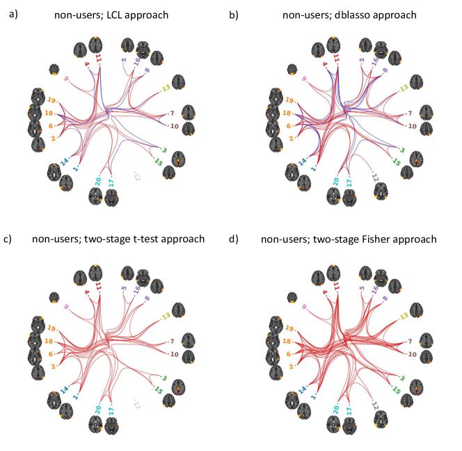
Figure 5: Brain sub-networks in non-users as estimated with the a: LCL approach; b: dblasso approach; c two-stage t-test approach; d two-stage Fisher approach. We present the results only for the nodes we selected in Figure 4. Only edges with p-value $<1\times 10^{-13}$ are presented. Red edges represent positive edge strength, and blue edges represent negative edge strength. For two-stage approaches, the edges are tested without computing population-level edge estimates, so we plot all the edges in red.

From an estimation accuracy perspective, for the non-user group, dblasso estimated 1754 edges (8.8%) as significant connections among 200 brain nodes and LCL detects 1326 edges (6.7%); 2648 edges (13.3%) and 1414 edges (7.1%) are detected by two-stage t-test and two-stage Fisher approaches, respectively. The larger number of significant edges detected by dblasso and two-stage t-test is likely due to the inflated type-I error, as illustrated in our simulations when subject-specific heterogeneity is present in the data. We illustrate in Figure 5 the most significant edges (p-values $<1\times 10^{-13}$) detected by LCL, dblasso, two-stage t-test and two-stage Fisher among the previously selected brain nodes. While the overall patterns of connectivity are similar among these methods when compared to the proposed method, the stark difference in the number of detected edges by dblasso and two-stage t-test highlights the importance of modeling the heterogeneity in functional connectivity studies even when the population-level connectivity is of interest. We note that with $200$ nodes and $120$ observations per subject, LCL is not able to estimate the variances of the network edges.

7 Discussion

Motivated by the problem of inferring population-level edges in subject-varying GGMs, we proposed an estimation and inference framework for fixed effect parameters in doubly high-dimensional LMMs. As shown in our numerical studies, ignoring the subject-level variations in GGMs can result in highly-inflated type-I errors and false discoveries, even when the population-level network is of main interest. However, because of correlation and overlap between fixed and random effect covariates, previous works on high-dimensional LMMs, including Li et al. (2021), do not apply to the GGM setting and may suffer from inflated type-I error and insufficient coverage of confidence intervals. Our estimation and inference framework for doubly high-dimensional LMMs addresses these challenges, while also allowing a larger number of random effects than the number of observations per subject. We also proposed a new moment-based penalized variance component estimator, which addresses the challenges of estimating variance components in doubly high-dimensional LMMs.

Similar to Li et al. (2021), we treat the parameter $a$ in the proxy covariance matrix as a tuning parameter and use a cross-validation procedure to select $a$. However, our theoretical results hold for any positive value of the constant $a$, and, in practice, we can simply set $a$ to an arbitrary constant. Our additional simulation studies in Appendix F.2 explore the effect of $a$ on the finite sample performance of the proposed method and show that, for any constant $a>0$, the proposed method has correct confidence interval coverage and controls the type-I error. However, the value of $a$ may impact the power of detecting non-zero $\beta_{l}$ and the estimation accuracy of $\beta$ and the variance components.

A novel aspect of the proposed method, compared with the existing procedures, is that it accommodates subject-varying covariance matrices. This is a crucial feature for handling graphical modeling with subject-level heterogeneity. Our theoretical analysis avoids making specific distributional assumptions, allowing for a broad spectrum of potential covariance matrix distributions to be considered. Exploring these diverse choices could be an interesting direction for future research.

Two other extensions of our framework could be of interest. First, motivated by our GGM problem, we focused on the setting where the fixed and random effect design matrices are identical. We also assumed $p/m>c_{0}>1$ for some constant $c_{0}$. In the Appendix B–E, we extend our framework to generic doubly high-dimensional LMMs, where the random effect covariates are a subset of the fixed effect covariates. Assuming fewer random than fixed effect covariates ($q\leq p$), we show that our framework works if $\lim_{q,m\xrightarrow{}\infty}q/m\neq 1$. However, these results are based on unified proof techniques for $q/m>c_{0}>1$ and $q/m<c_{1}<1$, with techniques specifically designed for the case $q/m>c_{0}>1$. Therefore, our assumptions for the setting $q/m<c_{1}<1$ could be relaxed and our rates may not be optimal. Secondly, our framework extends beyond independent and identically distributed noise terms. The proposed method readily accommodates observations featuring correlated noise terms and seamlessly extends to mixed-effect vector autoregressive models. This makes the mode a versatile tool that can be directly employed in the analysis of time series observations in certain settings.

In summary, our framework provides rigorous inference of brain connectivity networks in the presence of subject heterogeneity during multi-subject experiments. It facilitates a systematic exploration of population-level brain network structures, enhancing our understanding of the functionalities associated with various brain regions. It aids in identifying crucial brain regions, such as those highly connected with many others, providing targeted avenues for further investigations. Additionally, it helps detecting AD-induced alterations in brain connectivity patterns Lee et al. (2016). Beyond its utility in resting-state fMRI data, our framework is directly applicable to task-based fMRI signals. This adaptability is particularly beneficial in scenarios where substantial differences in brain functional connectivity are expected between distinct groups Zhao et al. (2023).

Appendix A Outline

In the main discussion, we have established an estimation and inference framework for doubly high-dimensional linear mixed models (LMMs) in the context of neighborhood-based graphical modeling of heterogeneous data. In that specific setting, the fixed and the random effects had identical design matrices. However, doubly high-dimensional LMMs may also arise from settings where the two matrices are not identical, but yet share a set of variables or have highly correlated columns, therefore still violating assumptions on the conditional independence of the fixed and random design matrices. A typical example is in longitudinal data analysis with random slope models — if we want to allow random slopes for a large number of explanatory variables, we end up with a doubly high-dimensional LMM. With advancing technology allowing us to collect more variables than ever, such examples will only become more ubiquitous. Thus, we extend our framework to a generic doubly high-dimensional LMM, formulated as:

$$y^{i}=X^{i}\beta+Z^{i}\gamma_{i}+\epsilon_{i},\quad i=1,\dots,n.$$ (12)

Here, each $y^{i}\in\mathop{\mathbb{R}}^{m}$ is the observation vector, $X^{i}\in\mathop{\mathbb{R}}^{m\times p}$ and $Z^{i}\in\mathop{\mathbb{R}}^{m\times q}$ are the design matrices, where $X^{i}\mid\Sigma_{X}^{i}\sim MN_{m\times p}(0,I_{m},\Sigma_{X}^{i})$ and $Z^{i}\mid\Sigma_{Z}^{i}\sim MN_{m\times q}(0,I_{m},\Sigma_{Z}^{i})$. The subject-level covariance matrices $\Sigma_{X}^{i}$ and $\Sigma_{Z}^{i}$ are centered at the population-level covariance matrices $\Sigma_{X}$, $\Sigma_{Z}$, respectively. We assume the $q$ random effect covariates are a subset of the $p$ fixed effect covariates. Moreover, we assume that conditional on $X^{i}$, the random effect coefficients $\gamma_{i}\in\mathop{\mathbb{R}}^{q}$ and the noise term $\epsilon_{i}\in\mathop{\mathbb{R}}^{m}$ are independent with variance $\Psi$ and $\mathop{\mathbb{R}}^{i}$, and satisfy $\gamma_{i}\in\mathop{\mathrm{SGV}}(c_{1}\|\Psi\|_{2})$, $\epsilon_{i}\in\mathop{\mathrm{SGV}}(c_{2}\|R^{i}\|_{2})$, respectively. We allow for either $q>c_{0}m$ or $m>c_{0}q$, for some constant $c_{0}>1$. The fixed effect coefficients $\beta$ has support $S$ with cardinality $s$.

We present the estimators, the inference framework and their theoretical properties in the Appendix B–E, with the proofs available upon request. All results are directly applicable to the doubly high-dimensional LMM in (2) of the main paper in the context of graphical model selection, where we simply need to set $X^{i}=Z^{i}$.

We define some relevant quantities to facilitate the discussion. We use $\mathbf{1}\{\cdot\}$ to represent the indicator function. The proxy covariance matrix is denoted by $\Sigma_{a}^{i}=aZ^{i}(Z^{i})^{\top}+I_{m}$ and $\Sigma_{a}=\mathop{\mathrm{diag}}\left(\{\Sigma_{a}^{i}\}_{i=1}^{n}\right)$. The vectors/matrices $y$, $\gamma$, $\epsilon$ and $X$ are formed by vertically stacking the vectors/matrices $y^{i}$’s, $\gamma_{i}$’s, $\epsilon_{i}$’s and $X^{i}$’s respectively. A random variable $X$ is sub-exponential with parameters $(a,b)$ if $\forall\ |t|\leq 1/b$, $\mathop{\mathbb{E}}(\exp(tX))\leq\exp(at^{2}/2)$. We define $\mathop{\mathrm{SE}}(a,b)$ as the class of all sub-exponential random variables with mean zero and parameters $(a,b)$. Denote $e_{j}$ as a length $q$ unite vector with the $j$th entry taking value $1$.

Appendix B Fixed Effect Estimator $\hat{\beta}$

We define the estimator $\hat{\beta}$ for the fixed effect coefficients $\beta$ in model (12) as follows:

$$\hat{\beta}=\operatorname*{\arg\!\min}_{\beta\in\mathbb{R}^{p}}{\left(2\mathop{\mathrm{tr}}(\Sigma_{a}^{-1})\right)}^{-1}\|\Sigma_{a}^{-1/2}(y-X\beta)\|_{2}^{2}+\lambda_{a}\|\beta\|_{1}.$$

We state a generalized version of Theorem 1 of the main paper and its related assumptions for the generic doubly high-dimensional LMM in (12):

Assumption 6.

1. Let $q>c_{0}m$ or $m>c_{0}q$ for some constant $c_{0}>1$ and let $m\vee q>c_{1}$ for some suitably large constant $c_{1}>0$. Moreover, let $\log(q)\left(q/m\right)^{\mathop{\mathbf{1}\{q>c_{0}m\}}}/n=o(1)$.

2. $\forall\ i$, $\sigma(\Sigma_{X})\asymp\sigma(R^{i})\asymp\|\Psi\|_{2}\asymp 1$, $\|\Sigma_{X}^{i}-\Sigma_{X}\|_{2}\leq\sigma_{\min}(\Sigma_{X})-c_{2}$, for some constant $c_{2}>0$.

Assumption 6.2 implies $\sigma(\Sigma_{X}^{i})\asymp 1$ for all $i=1,\dots,n$ (Weyl’s theorem, Bhatia (2007)).

Assumption 7.

1. $\Psi=\mathop{\mathrm{diag}}(\psi)$ for a vector $\psi\in\mathop{\mathbb{R}}^{q}$. The support of $\psi$ is $S_{\psi}$ with cardinality $s_{\psi}<c_{2}m\wedge n$ for some constant $c_{2}>0$, and $\min(\psi_{S_{\psi}})\asymp\max(\psi_{S_{\psi}})\asymp 1$.

2. $\sigma_{\min}(\Psi)\asymp 1$.

Theorem 6 (Fixed effect estimator consistency).

Under Assumption 6.1 and Assumption 6.2, with probability at least $1-4\exp\{-cn\}-12\exp\{-c\log(n)\}-2\exp\{-cmnq^{-\mathop{\mathbf{1}\{q>c_{0}m\}}}\}-\exp\{-cn(m/q)^{\mathop{\mathbf{1}\{q>c_{0}m\}}}\}$, we have the following results:

1. When $q>c_{0}m$: Taking $\lambda_{a}=c_{1}\sqrt{q\log(p)/(nm)}$ for a suitably large $c_{1}>0$, we have that:

   $$\|\hat{\beta}-\beta^{*}\|_{2}=O_{p}\left(\sqrt{\frac{sq\log(p)}{mn}}\right),$$

   $$\|\hat{\beta}-\beta^{*}\|_{1}=O_{p}\left(s\sqrt{\frac{q\log(p)}{mn}}\right),$$

   $$\left\|\Sigma_{a}^{-1/2}X(\hat{\beta}-\beta^{*})\right\|_{2}^{2}=O_{p}\left(s\log(p)\right).$$

2. When $q>c_{0}m$ and Assumption 7.1 also holds: Taking $\lambda_{a}=c_{2}\sqrt{\log(p)\log^{2}(n)/n}$ for suitably large $c_{2}>0$, we have that:

   $$\|\hat{\beta}-\beta^{*}\|_{2}=O_{p}\left(\sqrt{\frac{s\log^{2}(n)\log(p)}{n}}\right),$$

   $$\|\hat{\beta}-\beta^{*}\|_{1}=O_{p}\left(s\sqrt{\frac{\log^{2}(n)\log(p)}{n}}\right),$$

   $$\|\Sigma_{a}^{-1/2}X(\hat{\beta}-\beta^{*})\|_{2}^{2}=O_{p}\left(\frac{sm\log^{2}(n)\log(p)}{q}\right).$$

3. When $m>c_{0}q$ and $p=q$: Taking $\lambda_{a}=c_{3}\sqrt{\log(p)/(nm^{2})}$ for suitably large $c_{3}>0$, we have that:

   $$\|\hat{\beta}-\beta^{*}\|_{2}=O_{p}\left(\sqrt{\frac{s\log(p)}{n}}\right),$$

   $$\|\hat{\beta}-\beta^{*}\|_{1}=O_{p}\left(s\sqrt{\frac{\log(p)}{n}}\right),$$

   $$\|\Sigma_{a}^{-1/2}X(\hat{\beta}-\beta^{*})\|_{2}^{2}=O_{p}\left(s\log(p)\right).$$

4. When $m>c_{0}q$ and $p>q$: Taking $\lambda_{a}=c_{4}\sqrt{{\log(p)}/{(nm)}}$ for suitably large $c_{4}>0$, we have that:

   $$\|\hat{\beta}-\beta^{*}\|_{2}=O_{p}\left(\sqrt{\frac{sm\log(p)}{n}}\right),$$

   $$\|\hat{\beta}-\beta^{*}\|_{1}=O_{p}\left(s\sqrt{\frac{m\log(p)}{n}}\right),$$

   $$\|\Sigma_{a}^{-1/2}X(\hat{\beta}-\beta^{*})\|_{2}^{2}=O_{p}\left(sm\log(p)\right).$$

B.1 Related lemmas for Theorem 6

Lemma 7 (Core Lemma).

Assume $q>c_{0}m$ or $m>c_{0}q$ for some constant $c_{0}>1$. $Z$ is a $m\times q$ matrix with entries independently following the $N(0,1)$ distribution, and $Z^{i}$, $i=1,\dots,n$ are identical copies of $Z$. Then the following properties hold for the non-zero singular values $\sigma(Z)$ of $Z$ and $\sigma(Z^{i})$ of $Z^{i}$’s:

1. $|\sqrt{q}-\sqrt{m}|\leq\mathop{\mathbb{E}}(\sigma(Z))\leq\sqrt{m}+\sqrt{q}$, $\mathop{\mathbb{E}}(\sigma(Z))\asymp\sqrt{m}\vee\sqrt{q}$.

2. $\sigma(Z)-\mathop{\mathbb{E}}(\sigma(Z))\in\mathop{\mathrm{SG}}(1)$.

3. $\mathop{\mathbb{E}}(\sigma^{2}(Z))\in[\mathop{\mathbb{E}}(\sigma(Z))^{2},\mathop{\mathbb{E}}(\sigma(Z))^{2}+1]$, $\mathop{\mathbb{E}}(\sigma^{2}(Z))\asymp m\vee q$.

4. $\sigma^{2}(Z)-\mathop{\mathbb{E}}(\sigma^{2}(Z))\in\mathop{\mathrm{SE}}(32,4)$. $\sum_{i=1}^{n}\sigma^{2}(Z^{i})\asymp n(m\vee q)$ with probability at least $1-2\exp\{-c_{1}n(m\vee q)\}$, for some $c_{1}>0$.

Further assume $m\vee q>c_{2}>0$ for some suitably large constant $c_{2}$. Denote $\Sigma_{a}^{i}=aZ^{i}(Z^{i})^{\top}+I_{m}$, where $a$ is a positive constant. Then we have the following properties hold for any constant $c>0$, for positive constants $c_{3},c_{4},\dots$:

1. $\frac{1}{\mathop{\mathbb{E}}(\sigma^{2}(Z))+c}\leq\mathop{\mathbb{E}}\left(\frac{1}{\sigma^{2}(Z)+c}\right)\leq\frac{4}{\mathop{\mathbb{E}}(\sigma^{2}(Z))+c}$.

2. $\frac{1}{\sigma^{2}(Z)+c}-\mathop{\mathbb{E}}\left(\frac{1}{\sigma^{2}(Z)+c}\right)\in\mathop{\mathrm{SE}}\left(c_{3}\mathop{\mathbb{E}}\left(\frac{1}{\sigma^{2}(Z)+c}\right)^{2},c_{3}\mathop{\mathbb{E}}\left(\frac{1}{\sigma^{2}(Z)+c}\right)\right)$.

3. $\sum_{i=1}^{n}\frac{1}{\sigma^{2}(Z^{i})+c}\asymp\frac{n}{m\vee q}$ with probability at least $1-2\exp\{-c_{4}n\}$. $\max_{1\leq i\leq n}\frac{1}{\sigma^{2}(Z^{i})+c}\leq\frac{1}{c}\wedge\frac{c_{5}\log(n)}{m\vee q}$ with probability at least $1-2\exp\{-c_{6}\log(n)\}$, $\min_{1\leq i\leq n}\frac{1}{\sigma^{2}(Z^{i})+c}\geq\frac{c_{7}}{\log(n)+m\vee q}$ with probability at least $1-2\exp\{-c_{6}\log(n)\}$.

4. $\sum_{i=1}^{n}\mathop{\mathrm{tr}}\left((\Sigma_{a}^{i})^{-1}\right)\asymp mnq^{-\mathop{\mathbf{1}\{q>c_{0}m\}}}$ with probability at least $1-4\exp\{-c_{8}n\}$.
   When $q>c_{0}m$: $\frac{c_{9}m}{\log(n)+q}\leq\min_{i}\mathop{\mathrm{tr}}\left((\Sigma_{a}^{i})^{-1}\right)\leq\max_{i}\mathop{\mathrm{tr}}\left((\Sigma_{a}^{i})^{-1}\right)\leq c_{10}m\left(1\wedge\frac{\log(n)}{q}\right)$ with probability at least $1-4\exp\{-c_{11}\log(n)\}$.
   When $m>c_{0}q$: $c_{12}\left(m+\frac{q}{m+\log(n)}\right)\leq\min_{i}\mathop{\mathrm{tr}}\left((\Sigma_{a}^{i})^{-1}\right)\leq\max_{i}\mathop{\mathrm{tr}}\left((\Sigma_{a}^{i})^{-1}\right)$
   $\leq c_{13}\left(m+q\left(1\wedge\frac{\log(n)}{m}\right)\right)$ with probability at least $1-4\exp\{-c_{14}\log(n)\}$.

5. $\mathop{\mathbb{E}}\left(Z^{\top}(aZZ^{\top}+I_{m})^{-1}Z\right)=kI_{q}$, $k\asymp\left({m}/{q}\right)^{\mathop{\mathbf{1}\{q>c_{0}m\}}}$. $\sigma\left(\sum_{i=1}^{n}(Z^{i})^{\top}(\Sigma_{a}^{i})^{-1}Z^{i}\right)\asymp n\left({m}/{q}\right)^{\mathop{\mathbf{1}\{q>c_{0}m\}}}$ with probability at least $1-\exp\left\{\log(q)-c_{16}n\left({m}/{q}\right)^{\mathop{\mathbf{1}\{q>c_{0}m\}}}\right\}$.

6. Assume ${\log(q)}\left(q/m\right)^{\mathop{\mathbf{1}\{q>c_{0}m\}}}/n=o(1)$. Then with probability at least $1-2\exp\{-c_{18}n\}-2\exp\{-c_{18}\log(n)\}-\exp\left\{-c_{18}n\left(m/q\right)^{\mathop{\mathbf{1}\{q>c_{0}m\}}}\right\}$:

   $$\sigma\left(\sum_{i=1}^{n}(Z^{i})^{\top}(\Sigma_{a}^{i})^{-2}Z^{i}\right)\leq\begin{cases}c_{17}\frac{n}{q}\left(1\wedge\frac{m\log(n)}{q}\right)&,q>c_{0}m,\\ c_{17}\frac{n}{m}&,m>c_{0}q.\end{cases}$$

Lemma 8.

1. Under Assumption 6.1 and Assumption 6.2, with probability at least $1-4\exp\{-cn\}-2\exp\{-c\log(n)\}-2\exp\{-cmnq^{-\mathop{\mathbf{1}\{q>c_{0}m\}}}\}-\exp\left\{-cn\left(m/q\right)^{\mathop{\mathbf{1}\{q>c_{0}m\}}}\right\}$, we have:

   $$\begin{cases}\sigma(X^{\top}\Sigma_{a}^{-1}X)\asymp\frac{mn}{q}&,q>c_{0}m,\\ \sigma(X^{\top}\Sigma_{a}^{-1}X)\asymp n&,m>c_{0}q\text{ and }p=q,\\ c_{1}n\leq\sigma(X^{\top}\Sigma_{a}^{-1}X)\leq c_{2}mn&,m>c_{0}q\text{ and }q<p.\end{cases}$$

2. Under Assumption 6.1 and Assumption 6.2, $\max_{i}\sigma((X^{i})^{\top}(\Sigma^{i}_{a})^{-1}X^{i})\leq c_{1}$ when $p=q$; when $p>q$, with probability at least $1-8\exp\{-c_{2}\log(n)\}$ we have:

   $$\max_{i}\sigma((X^{i})^{\top}(\Sigma^{i}_{a})^{-1}X^{i})\leq\begin{cases}c_{3}\left(1\vee\frac{m\log^{2}(n)}{q}\right)&,q>c_{0}m,\\ c_{3}m\log^{2}(n)&,m>c_{0}q.\end{cases}$$

Lemma 9.

1. Under Assumption 6.1 and Assumption 6.2, we have

   $$\max_{1\leq j\leq p}\sum_{i=1}^{n}\left\|(Z^{i})^{\top}\left(\Sigma_{a}^{i}\right)^{-1}X_{j}^{i}\right\|_{2}^{2}\left\|\Psi\right\|_{2}+\left\|\left(\Sigma_{a}^{i}\right)^{-1}X_{j}^{i}\right\|_{2}^{2}\|R^{i}\|_{2}\leq\begin{cases}c_{1}\frac{nm}{q}&,q>c_{0}m,\\ c_{1}n&,m>c_{0}q\text{ and }q=p,\\ c_{1}mn&,m>c_{0}q\text{ and }q<p,\end{cases}$$

   with probability at least $1-4\exp\{-cn\}-12\exp\{-c\log(n)\}-2\exp\{-cmnq^{-\mathop{\mathbf{1}\{q>c_{0}m\}}}\}-\exp\{-cn(m/q)^{\mathop{\mathbf{1}\{q>c_{0}m\}}}\}$.

   If we additionally assume Assumption 7.1, we have

   $$\max_{1\leq j\leq p}\sum_{i=1}^{n}\left\|(Z^{i}_{S_{\psi}})^{\top}\left(\Sigma_{a}^{i}\right)^{-1}X_{j}^{i}\right\|_{2}^{2}\left\|\Psi\right\|_{2}+\left\|\left(\Sigma_{a}^{i}\right)^{-1}X_{j}^{i}\right\|_{2}^{2}\|R^{i}\|_{2}\leq\begin{cases}\frac{c_{1}mn}{q}\left(1\wedge\frac{m\log^{2}(n)}{q}\right),&\\ \quad\quad q>c_{0}m,&\\ c_{1}n,&\\ \quad\quad m>c_{0}q\text{ and }p=q,&\\ c_{1}mn,&\\ \quad\quad m>c_{0}q\text{ and }q<p,&\end{cases}$$

   with probability at least $1-4\exp\{-cn\}-6\exp\{-c\log(n)\}-2\exp\{-cmnq^{-\mathop{\mathbf{1}\{q>c_{0}m\}}}\}-\exp\left\{-cn\left(m/q\right)^{\mathop{\mathbf{1}\{q>c_{0}m\}}}\right\}$.

2. Define

   $$z_{0}^{*}=\max_{1\leq j\leq p}\left|\frac{1}{\mathop{\mathrm{tr}}(\Sigma_{a}^{-1})}X^{\top}_{j}\Sigma_{a}^{-1}(y-X\beta^{*})\right|.$$

   Under Assumption 6.1 and Assumption 6.2, we have

   $$z_{0}^{*}\leq\begin{cases}c_{1}\sqrt{\frac{q\log(p)}{nm}}&,q>c_{0}m,\\ c_{1}\sqrt{\frac{\log(p)\log^{2}(n)}{n}}&,q>c_{0}m\text{ and Assumption~{}\ref{as.A.add}.\ref{as.A.3}}alsoholds,\\ c_{1}\sqrt{\frac{\log(p)}{nm^{2}}}&,m>c_{0}q\text{ and }p=q,\\ c_{1}\sqrt{\frac{\log(p)}{nm}}&,m>c_{0}q\text{ and }p>q.\\ \end{cases}$$

   with probability at least $1-4\exp\{-cn\}-12\exp\{-c\log(n)\}-2\exp\{-cmnq^{-\mathop{\mathbf{1}\{q>c_{0}m\}}}\}-\exp\left\{-cn\left(m/q\right)^{\mathop{\mathbf{1}\{q>c_{0}m\}}}\right\}$.

Appendix C Inference Framework for $\beta$

Inference for $\beta$ is based on the de-biased LASSO framework. We follow the same procedure as introduced in Section 2 of the main paper, with slight modification in the context of a generic doubly high-dimensional LMM. To infer $\beta_{j}$, we first define the de-biased estimator $\hat{\beta}^{(db)}_{j}$:

$$\hat{\beta}_{j}^{(db)}=\hat{\beta}_{j}+\frac{\sum_{i=1}^{n}(\hat{w}_{j}^{i})^{\top}(\Sigma_{b}^{i})^{-1/2}(y^{i}-X^{i}\hat{\beta})}{\sum_{i=1}^{n}(\hat{w}_{j}^{i})^{\top}(\Sigma_{b}^{i})^{-1/2}X^{i}_{j}}.$$ (13)

Here, the modified proxy matrices $(\Sigma_{b}^{i})^{-1/2}$ are defined as:

$$\Sigma_{b}^{i}=aZ^{i}_{-j}(Z^{i}_{-j})^{\top}+I_{m},$$

$$\Sigma_{b}=\mathop{\mathrm{diag}}\left(\left\{\Sigma_{b}^{i}\right\}_{i=1}^{n}\right),$$

where with some abuse of notation, we define $Z^{i}_{-j}$, $j=1,\dots,q$ as the sub-matrix of $Z^{i}$ obtained by dropping the $j$th column of $Z^{i}$, and $Z^{i}_{-j}=Z^{i}$ for $j>q$. The projection orthogonal vector $w^{i}_{j}$ is defined as

$$\hat{w}^{i}_{j}=(\Sigma_{b}^{i})^{-1/2}\left(X^{i}_{j}-X^{i}_{-j}\hat{\kappa}_{j}\right)$$

and the projection vector $\hat{\kappa}_{j}$ is defined as

$$\hat{\kappa}_{j}=\operatorname*{\arg\!\min}_{\kappa_{j}\in\mathbb{R}^{p-1}}\left({2\mathop{\mathrm{tr}}\left(\Sigma_{b}^{-1}\right)}\right)^{-1}\|\Sigma_{b}^{-1/2}\left(X_{j}-X_{-j}\kappa_{j}\right)\|_{2}^{2}+\lambda_{j}\|\kappa_{j}\|_{1}.$$

We state here the generalized version of Theorem 2 of the main paper and its related assumptions for the generic doubly high-dimensional LMM in (12):

Assumption 8.

1. $\log(p)=o(mn)$. $\forall\ j=1,\dots,p$, conditional on $X^{i}_{-j}$, the random vector $X^{i}_{j}$ has mean $X^{i}_{-j}\kappa_{j}^{*}$ for $\kappa_{j}^{*}\in\mathop{\mathbb{R}}^{p-1}$ and variance $G_{j}$, and $X^{i}_{j}-X^{i}_{-j}\kappa_{j}^{*}\mid X^{i}_{-j}\in\mathop{\mathrm{SGV}}(c_{1}\|G_{j}\|_{2})$. The support for $\kappa_{j}^{*}$ is $H_{j}$ and its cardinality is $|H_{j}|$. Assume $\|\kappa_{j}^{*}\|_{1}\leq c_{1}|H_{j}|$.

2. $\frac{\|G_{j}\|_{2}}{\sigma_{\min}(G_{j})}\log(n)\sqrt{1\wedge\frac{\log(n)}{m\vee q}}\leq c_{1}\sqrt{mnq^{-\mathop{\mathbf{1}\{q>c_{0}m\}}}}$

3. 1. When $q>c_{0}m$, $p=q$:

      $$\frac{|H_{j}|q^{2}\log(p)}{m^{3}n}\ll\|G_{j}\|_{2}\leq c_{1}\frac{mn}{\log(n)\log(p)}$$ (14)

      $$\frac{\|G_{j}\|_{2}}{\sigma_{\min}^{2}(G_{j})}\ll\frac{mn}{|H_{j}|^{3}\log(n)\log(p)}\wedge\frac{m^{2}n^{2}}{s^{2}|H_{j}|q\log(n)\log^{2}(p)}$$ (15)

      $$\frac{\|G_{j}\|_{2}}{\sigma_{\min}(G_{j})}\ll\frac{mn}{|H_{j}|\log(n)\log(p)}$$ (16)

   2. when $q>c_{0}m$, $p>q$: assume the conditions (14)–(16), and additionally assume $\|G_{j}\|_{2}\gg\frac{|H_{j}|\log(p)\log^{3}(n)}{mn}$

   3. When $m>c_{0}q$:

      $$\frac{|H_{j}|\log(p)}{m^{3}n}\left({m^{3}\log^{5}(n)}\right)^{\mathbf{1}\{p>q\}}\ll\|G_{j}\|_{2}\leq c_{1}\frac{mn}{\log(p)}\left(\frac{1}{m\log(n)}\right)^{\mathbf{1}\{p>q\}}$$

      $$\frac{\|G_{j}\|_{2}}{\sigma_{\min}^{2}(G_{j})}\ll\left(\frac{m^{3}n}{|H_{j}|^{3}\log(p)}\left(\frac{1}{m\log^{2}(n)}\right)^{\mathbf{1}\{p>q\}}\right)\wedge\left(\frac{m^{3}n^{2}}{s^{2}|H_{j}|\log^{2}(p)}\left(\frac{1}{m^{2}\log^{2}(n)}\right)^{\mathbf{1}\{p>q\}}\right)$$

      $$\frac{\|G_{j}\|_{2}}{\sigma_{\min}(G_{j})}\ll\frac{m^{2}n}{|H_{j}|\log(p)}\left(\frac{1}{m\log(n)}\right)^{\mathbf{1}\{p>q\}}$$

Assumption 9.

1. Condition 1: When Assumption 7.2 holds:

   $$\begin{cases}\frac{\|G_{j}\|_{2}}{\sigma_{\min}(G_{j})}\ll\frac{n}{\log^{6}(n)}&,\ q>c_{0}m\\ \frac{\|G_{j}\|_{2}}{\sigma_{\min}(G_{j})}\ll\frac{n}{\log^{5}(n)}&,\ m>c_{0}q\end{cases}$$

2. Condition 2: When Assumption 7.1 holds and $j\in S_{\psi}$:

   $$\begin{cases}\frac{\|G_{j}\|_{2}}{\sigma^{2}_{\min}(G_{j})}\ll\frac{n}{\log^{6}(n)}&,\ q>c_{0}m\\ \frac{\|G_{j}\|_{2}}{\sigma^{2}_{\min}(G_{j})}\ll\frac{mn}{\log^{5}(n)}&,\ m>c_{0}q\end{cases}$$

3. Condition 3: When Assumption 7.1 holds and $j\not\in S_{\psi}$:

   $$\begin{cases}\frac{\|G_{j}\|_{2}}{\sigma_{\min}(G_{j})}\ll\frac{n}{s_{\psi}\log^{7}(n)}\wedge\frac{n^{2}}{s_{\psi}|H_{j}|^{2}\log(p)\log^{8}(n)}\wedge\frac{n}{\log^{6}(n)}&,\ q>c_{0}m\\ \frac{\|G_{j}\|_{2}}{\sigma_{\min}(G_{j})}\ll\frac{mn^{2}}{s_{\psi}|H_{j}|^{2}\log(p)\log^{7}(n)}\wedge\frac{n}{\log^{5}(n)}&,\ m>c_{0}q,\ p=q\\ \frac{\|G_{j}\|_{2}}{\sigma_{\min}(G_{j})}\ll\frac{n^{2}}{s_{\psi}|H_{j}|^{2}\log(p)\log^{8}(n)}\wedge\frac{n}{\log^{5}(n)}&,\ m>c_{0}q,\ p>q\end{cases}$$

As discussed in the main paper, the bound $\|\kappa_{j}^{*}\|_{1}\leq c_{1}|H_{j}|$ is satisfied when $\Sigma_{X}^{i}=\Sigma_{X}$. The variance $G_{j}$ may take any form as long as its singular values satisfy Assumption 8 and Assumption 9. If we were to assume that $G_{j}$ takes the same “sandwich” form as $\Sigma_{\theta}^{i}$ such that $G_{j}=Z_{-j}\Psi^{j}(Z_{-j})^{\top}+R^{i,j}$ for some matrix $\Psi^{j}\in\mathop{\mathbb{R}}^{(p-1)\times(p-1)}$ and $R^{i,j}\in\mathop{\mathbb{R}}^{m\times m}$, we could bound $\sigma(G_{j})$ based on the rates of $\sigma\left(\Sigma_{\theta}^{i}\right)$: assuming that $\sigma\left(R^{i,j}\right)\asymp 1$, and $\Psi^{j}$ takes the same form as $\Psi$ (i.e., $\sigma\left(\Psi^{j}\right)\asymp 1$ as in Assumption 7.2, or $\Psi^{j}$ is a sparse diagonal matrix as in Assumption 7.1), we would have $\sigma_{\min}(G_{j})\asymp\sigma_{\min}(\Sigma_{\theta}^{i})$ and $\|G_{j}\|_{2}\asymp\|\Sigma_{\theta}^{i}\|_{2}$, and the following results bound $\sigma\left(\Sigma_{\theta}^{i}\right)$:

Lemma 10.

For $\Sigma_{\theta}^{i}=Z^{i}\Psi(Z^{i})^{\top}+R^{i}$, $i\in\{1,\dots,n\}$, under Assumption 6, with probability at least $1-c_{1}\exp\{-c_{2}m\}$, we have:

1. When $m>c_{0}q$: Under either Assumption 7.1 or Assumption 7.2,

   $$c_{3}\leq\sigma_{\min}(\Sigma_{\theta}^{i})\leq\sigma_{\max}(\Sigma_{\theta}^{i})\leq c_{4}m.$$

2. When $q>c_{0}m$: Under Assumption 7.2,

   $$\sigma_{\min}(\Sigma_{\theta}^{i})\asymp\sigma_{\max}(\Sigma_{\theta}^{i})\asymp q.$$

   Under Assumption 7.1,

   $$c_{5}\leq\sigma_{\min}(\Sigma_{\theta})\leq\sigma_{\max}(\Sigma_{\theta})\leq c_{6}m.$$

Theorem 11.

Under Assumption 6, Assumption 8 and Assumption 9, with probability at least $1-c_{1}\exp\{-cn\}-c_{2}\exp\{-c\log(n)\}-c_{3}\exp\{-cmnq^{-\mathop{\mathbf{1}\{q>c_{0}m\}}}\}-c_{4}\exp\left\{-cn\left(m/q\right)^{\mathop{\mathbf{1}\{q>c_{0}m\}}}\right\}-c_{5}\exp\{-c\log(p)\}-c_{6}\exp\{-cmn\}$, we have that

$$\frac{1}{\sqrt{V_{j}}}\left(\hat{\beta}_{j}^{(db)}-\beta_{j}^{*}\right)=R_{j}+o_{p}(1),\quad\text{where }R_{j}\xrightarrow[]{d}N(0,1),$$

where the variance $V_{j}$ is given by

$$V_{j}=\frac{\sum_{i=1}^{n}(\hat{w}^{i}_{j})^{\top}(\Sigma_{b}^{i})^{-1/2}\Sigma_{\theta^{*}}^{i}(\Sigma_{b}^{i})^{-1/2}\hat{w}^{i}_{j}}{\left|\sum_{i=1}^{n}(\hat{w}^{i}_{j})^{\top}(\Sigma_{b}^{i})^{-1/2}X^{i}_{j}\right|^{2}}.$$

C.1 Related lemmas for Theorem 11

Lemma 12.

1. Define

   $$z_{j}^{*}:=\frac{1}{\mathop{\mathrm{tr}}(\Sigma_{b}^{-1})}\left\|X^{\top}_{-j}\Sigma_{b}^{-1}(X_{j}-X_{-j}\kappa_{j}^{*})\right\|_{\infty}.$$ (17)

   Under Assumption 6 and Assumption 8.1, with probability at least $1-2\exp\{-cmnq^{-\mathop{\mathbf{1}\{q>c_{0}m\}}}\}-4\exp\{-c\log(n)\}-4\exp\{-cn\}-2\exp\{-c\log(p)\}-\exp\{-cn(m/q)^{\mathop{\mathbf{1}\{q>c_{0}m\}}}\}$, we have that:

   $$z_{j}^{*}\leq\begin{cases}c_{1}\sqrt{\frac{q\log(p)\|G_{j}\|_{2}}{m^{2}n}\left(1\wedge\frac{m\log(n)}{q}\right)}&,q>c_{0}m\text{ and }q=p,\\ c_{1}\sqrt{\frac{\log(p)\|G_{j}\|_{2}}{m^{3}n}}&,m>c_{0}q\text{ and }q=p,\\ c_{1}\sqrt{\frac{q\log(p)\|G_{j}\|_{2}}{mn}\left(1\wedge\frac{\log(n)}{q}\right)}&,q>c_{0}m\text{ and }q<p,\\ c_{1}\sqrt{\frac{\log(p)\|G_{j}\|_{2}}{mn}\left(1\wedge\frac{\log(n)}{m}\right)}&,m>c_{0}q\text{ and }q<p.\end{cases}$$

2. Under Assumption 6 and Assumption 8.1, we have the following results with probability at least $1-c_{1}\exp\{-cn(m/q)^{\mathop{\mathbf{1}\{q>c_{0}m\}}}\}-c_{2}\exp\{-cn\}-c_{3}\exp\{-c\log(n)\}-c_{4}\exp\{-cmnq^{-\mathop{\mathbf{1}\{q>c_{0}m\}}}\}-c_{5}\exp\{-c\log(p)\}$:

   1. When $q=p$ and $q>c_{0}m$: $\lambda_{j}=c_{6}\sqrt{\frac{q\log(p)\|G_{j}\|_{2}}{m^{2}n}\left(1\wedge\frac{m\log(n)}{q}\right)}$ with suitably large $c_{6}>0$, and

      $$\|\hat{\kappa}_{j}-\kappa_{j}^{*}\|_{2}\leq c_{7}\sqrt{\frac{|H_{j}|q\log(p)\|G_{j}\|_{2}}{m^{2}n}\left(1\wedge\frac{m\log(n)}{q}\right)},$$

      $$\|\hat{\kappa}_{j}-\kappa_{j}^{*}\|_{1}\leq c_{7}|H_{j}|\sqrt{\frac{q\log(p)\|G_{j}\|_{2}}{m^{2}n}\left(1\wedge\frac{m\log(n)}{q}\right)},$$

      $$\|\Sigma_{b}^{-1/2}X_{-j}(\hat{\kappa}_{j}-\kappa_{j}^{*})\|_{2}^{2}\leq c_{7}|H_{j}|{\frac{\log(p)\|G_{j}\|_{2}}{m}\left(1\wedge\frac{m\log(n)}{q}\right)}.$$

   2. When $q=p$ and $m>c_{0}q$: $\lambda_{j}=c_{6}\sqrt{\frac{\log(p)\|G_{j}\|_{2}}{m^{3}n}}$ with suitably large $c_{6}>0$, and

      $$\|\hat{\kappa}_{j}-\kappa_{j}^{*}\|_{2}\leq c_{7}\sqrt{\frac{|H_{j}|\log(p)\|G_{j}\|_{2}}{mn}},$$

      $$\|\hat{\kappa}_{j}-\kappa_{j}^{*}\|_{1}\leq c_{7}|H_{j}|\sqrt{\frac{\log(p)\|G_{j}\|_{2}}{mn}},$$

      $$\|\Sigma_{b}^{-1/2}X_{-j}(\hat{\kappa}_{j}-\kappa_{j}^{*})\|_{2}^{2}\leq c_{7}|H_{j}|{\frac{\log(p)\|G_{j}\|_{2}}{m}}.$$

   3. When $q<p$ and $q>c_{0}m$: $\lambda_{j}=c_{6}\sqrt{\frac{q\log(p)\|G_{j}\|_{2}}{mn}\left(1\wedge\frac{\log(n)}{q}\right)}$ with suitably large $c_{6}>0$, and

      $$\|\hat{\kappa}_{j}-\kappa_{j}^{*}\|_{2}\leq c_{7}\sqrt{\frac{|H_{j}|q\log(p)\|G_{j}\|_{2}}{mn}\left(1\wedge\frac{\log(n)}{q}\right)},$$

      $$\|\hat{\kappa}_{j}-\kappa_{j}^{*}\|_{1}\leq c_{7}|H_{j}|\sqrt{\frac{q\log(p)\|G_{j}\|_{2}}{mn}\left(1\wedge\frac{\log(n)}{q}\right)},$$

      $$\|\Sigma_{b}^{-1/2}X_{-j}(\hat{\kappa}_{j}-\kappa_{j}^{*})\|_{2}^{2}\leq c_{7}|H_{j}|{\log(p)\|G_{j}\|_{2}\left(1\wedge\frac{\log(n)}{q}\right)}.$$

   4. When $q<p$ and $m>c_{0}q$: $\lambda_{j}=c_{6}\sqrt{\frac{\log(p)\|G_{j}\|_{2}}{mn}\left(1\wedge\frac{\log(n)}{m}\right)}$ with suitably large $c_{6}>0$, and

      $$\|\hat{\kappa}_{j}-\kappa_{j}^{*}\|_{2}\leq c_{7}\sqrt{\frac{|H_{j}|m\log(p)\|G_{j}\|_{2}}{n}\left(1\wedge\frac{\log(n)}{m}\right)},$$

      $$\|\hat{\kappa}_{j}-\kappa_{j}^{*}\|_{1}\leq c_{7}|H_{j}|\sqrt{\frac{m\log(p)\|G_{j}\|_{2}}{n}\left(1\wedge\frac{\log(n)}{m}\right)},$$

      $$\|\Sigma_{b}^{-1/2}X_{-j}(\hat{\kappa}_{j}-\kappa_{j}^{*})\|_{2}^{2}\leq c_{7}{{m\log(p)\|G_{j}\|_{2}}\left(1\wedge\frac{\log(n)}{m}\right)}.$$

3. Under Assumption 6 and Assumption 8.1, with probability at least $1-c_{1}\exp\{-cmnq^{-\mathop{\mathbf{1}\{q>c_{0}m\}}}\}-c_{2}\exp\{-c\log(n)\}-c_{3}\exp\{-cn\}-c_{4}\exp\{-c\log(p)\}-c_{5}\exp\{-cn(m/q)^{\mathop{\mathbf{1}\{q>c_{0}m\}}}\}-c_{6}\exp\{-cmn\}$, we have that:

   $$\|X_{-j}^{\top}\Sigma_{b}^{-1}X_{-j}(\hat{\kappa}_{j}-\kappa_{j}^{*})\|_{\infty}\leq\begin{cases}c_{7}\sqrt{|H_{j}|\frac{n\log(p)\|G_{j}\|_{2}}{q}\left(1\wedge\frac{m\log(n)}{q}\right)}&,q>c_{0}m\text{ and }q=p,\\ c_{7}\sqrt{|H_{j}|\frac{n\log(p)\|G_{j}\|_{2}}{m}}&,m>c_{0}q\text{ and }q=p,\\ c_{7}\sqrt{|H_{j}|\frac{mn\log(p)\|G_{j}\|_{2}}{q}\left(1\wedge\frac{\log(n)}{q}\right)}&,q>c_{0}m\text{ and }q<p,\\ c_{7}\sqrt{|H_{j}|n\log(p)\|G_{j}\|_{2}\left(m\wedge\log(n)\right)^{2}}&,m>c_{0}q\text{ and }q<p,\\ \end{cases}$$

4. Define

   $$w_{j} =\Sigma_{b}^{-1/2}(X_{j}-X_{-j}\kappa_{j}^{*})$$

   $$w^{i}_{j} =(\Sigma_{b}^{i}){-\frac{1}{2}}(X_{j}^{i}-X_{-j}^{i}\kappa_{j}^{*}).$$

   Under Assumption 6, Assumption 8.1 and Assumption 8.2, we have $c_{1}\sigma_{\min}(G_{j})nmq^{-\mathop{\mathbf{1}\{q>c_{0}m\}}}\leq\|w_{j}\|_{2}^{2}\leq c_{2}\sigma_{\max}(G_{j})nmq^{-\mathop{\mathbf{1}\{q>c_{0}m\}}}$ with probability at least $1-4\exp\{-cn\}-2\exp\{-c\log(n)\}$, and

   $$\max_{i}\|w^{i}_{j}\|_{2}^{2}\leq\begin{cases}c_{1}(m+\sqrt{m}\log(n))\left(1\wedge\frac{\log(n)}{q}\right)\|G_{j}\|_{2}&,q>c_{0}m,\\ c_{1}\left(m+\log(n)\sqrt{m\wedge{\log(n)}{}}\right)\|G_{j}\|_{2}&,m>c_{0}q\end{cases}$$

   with probability at least $1-6\exp\{-c\log(n)\}$.

5. Under Assumption 6, Assumption 8.1, Assumption 8.2, and Assumption 8.3, we have with probability at least $1-c_{1}\exp\{-cmnq^{-\mathop{\mathbf{1}\{q>c_{0}m\}}}\}-c_{2}\exp\{-c\log(n)\}-c_{3}\exp\{-cn\}-c_{4}\exp\{-c\log(p)\}-c_{5}\exp\{-cn(m/q)^{\mathop{\mathbf{1}\{q>c_{0}m\}}}\}-c_{6}\exp\{-cmn\}$ that

   $$|\hat{w}_{j}^{\top}\Sigma_{b}^{-1/2}X_{j}|\geq c_{7}\sigma_{\min}(G_{j})nmq^{-\mathop{\mathbf{1}\{q>c_{0}m\}}}.$$

6. Under Assumption 6 and Assumption 8, we have

   $$c_{1}\sigma_{\min}(G_{j})mnq^{-\mathop{\mathbf{1}\{q>c_{0}m\}}}\leq\|\hat{w}_{j}\|^{2}_{2}\leq c_{2}\sigma_{\max}(G_{j})nmq^{-\mathop{\mathbf{1}\{q>c_{0}m\}}},$$

   and

   $$\max_{i}\|\hat{w}_{j}^{i}\|_{2}^{2}\leq\begin{cases}c_{1}\left(m+\sqrt{m}\log(n)\right)\left(1\wedge\frac{\log(n)}{q}\right)\|G_{j}\|_{2}&,q>c_{0}m,\\ c_{1}\left(m+\log(n)\sqrt{m\wedge\log(n)}\right)\|G_{j}\|_{2}&,m>c_{0}q,\end{cases}$$

   with probability at least $1-c_{1}\exp\{-cmnq^{-\mathop{\mathbf{1}\{q>c_{0}m\}}}\}-c_{2}\exp\{-c\log(n)\}-c_{3}\exp\{-cn\}-c_{4}\exp\{-c\log(p)\}-c_{5}\exp\{-cn(m/q)^{\mathop{\mathbf{1}\{q>c_{0}m\}}}\}-c_{6}\exp\{-cmn\}$.

7. Under Assumption 6 and Assumption 8, with probability at least $1-c_{1}\exp\{-cmnq^{-\mathop{\mathbf{1}\{q>c_{0}m\}}}\}-c_{2}\exp\{-c\log(n)\}-c_{3}\exp\{-cn\}-c_{4}\exp\{-c\log(p)\}-c_{5}\exp\{-cn(m/q)^{\mathop{\mathbf{1}\{q>c_{0}m\}}}\}-c_{6}\exp\{-cmn\}$, we have the following results hold:

   1. Under Condition 1 defined in Assumption 9, we have

      $$\max_{i}\left\|(\Sigma_{\theta^{*}}^{i})^{1/2}(\Sigma_{b}^{i})^{-1/2}\hat{w}^{i}_{j}\right\|^{2}_{2}\leq\begin{cases}c_{1}\left(m+\sqrt{m}\log(n)\right)\left(1\wedge\frac{\log(n)}{q}\right)\log^{2}(n)\|G_{j}\|_{2},&\\ \quad\quad\quad\quad q>c_{0}m,\\ c_{1}\left(m+\log(n)\sqrt{m\wedge\log(n)}\right)\log^{2}(n)\|G_{j}\|_{2},&\\ \quad\quad\quad\quad m>c_{0}q,\end{cases}$$

      $$\hat{w}_{j}^{\top}\Sigma_{b}^{-1/2}\Sigma_{\theta^{*}}\Sigma_{b}^{-1/2}\hat{w}_{j}\geq c_{2}nmq^{-\mathop{\mathbf{1}\{q>c_{0}m\}}}\sigma_{\min}(G_{j}).$$

   2. Under Condition 2 defined in Assumption 9, we have

      $$\max_{i}\left\|(\Sigma_{\theta^{*}}^{i})^{1/2}(\Sigma_{b}^{i})^{-1/2}\hat{w}^{i}_{j}\right\|^{2}_{2}\leq\begin{cases}c_{1}\left(m+\sqrt{m}\log(n)\right)\left(1\wedge\frac{\log(n)}{q}\right)\log^{2}(n)\frac{m}{q}\|G_{j}\|_{2},&\\ \quad\quad\quad\quad q>c_{0}m,\\ c_{1}\left(m+\log(n)\sqrt{m\wedge\log(n)}\right)\log^{2}(n)\|G_{j}\|_{2},&\\ \quad\quad\quad\quad m>c_{0}q,\end{cases}$$

      $$\hat{w}_{j}^{\top}\Sigma_{b}^{-1/2}\Sigma_{\theta^{*}}\Sigma_{b}^{-1/2}\hat{w}_{j}\geq c_{2}nm^{2}q^{-2\times\mathop{\mathbf{1}\{q>c_{0}m\}}}\sigma_{\min}^{2}(G_{j}).$$

   3. Under Condition 3 defined in Assumption 9, we have

      $$\max_{i}\left\|(\Sigma_{\theta^{*}}^{i})^{1/2}(\Sigma_{b}^{i})^{-1/2}\hat{w}^{i}_{j}\right\|^{2}_{2}$$

      $$\leq c_{1}\begin{cases}&s_{\psi}\frac{m\log^{4}(n)}{q^{2}}\|G_{j}\|_{2}+s_{\psi}|H_{j}|^{2}\frac{m\log(p)\log^{5}(n)}{q^{2}n}\|G_{j}\|_{2}+\frac{m\log^{3}(n)}{q^{2}}\|G_{j}\|_{2}\\ &\quad\quad\quad\quad\quad\quad\quad\quad\quad\quad\quad\quad\quad\quad\quad\quad\quad\quad\quad,q>c_{0}m,\\ &s_{\psi}\frac{\log^{2}(n)}{m}\|G_{j}\|_{2}+s_{\psi}|H_{j}|^{2}\frac{\log(p)\log^{4}(n)}{mn}\|G_{j}\|_{2}+\log^{2}(n)\|G_{j}\|_{2}\\ &\quad\quad\quad\quad\quad\quad\quad\quad\quad\quad\quad\quad\quad\quad\quad\quad\quad\quad\quad,m>c_{0}q,\ p=q,\\ &s_{\psi}\frac{\log^{2}(n)}{m}\|G_{j}\|_{2}+s_{\psi}|H_{j}|^{2}\frac{\log(p)\log^{5}(n)}{n}\|G_{j}\|_{2}+\log^{2}(n)\|G_{j}\|_{2}\\ &\quad\quad\quad\quad\quad\quad\quad\quad\quad\quad\quad\quad\quad\quad\quad\quad\quad\quad\quad,m>c_{0}q,\ p>q\end{cases}$$

      $$\hat{w}_{j}^{\top}\Sigma_{b}^{-1/2}\Sigma_{\theta^{*}}\Sigma_{b}^{-1/2}\hat{w}_{j}\geq\begin{cases}c_{2}\frac{nm\sigma_{\min}(G_{j})}{q(q+\log(n))}&,q>c_{0}m,\\ c_{2}\frac{nm\sigma_{\min}(G_{j})}{m+\log(n)}&,m>c_{0}q,\end{cases}$$

Remark 13.

If we only assume $\|\Psi\|_{2}\leq c_{1}$ and do not restrict the structure of $\Psi$, we can still show

$$\max_{i}\left\|(\Sigma_{\theta^{*}}^{i})^{1/2}(\Sigma_{b}^{i})^{-1/2}\hat{w}^{i}_{j}\right\|^{2}_{2}\leq c_{1}m\log^{3}(n)\left(\log(n)/q\right)^{\mathop{\mathbf{1}\{q>c_{0}m\}}}\|G_{j}\|_{2}$$

$$\hat{w}_{j}^{\top}\Sigma_{b}^{-1/2}\Sigma_{\theta^{*}}\Sigma_{b}^{-1/2}\hat{w}_{j}\geq c_{2}nmq^{-\mathop{\mathbf{1}\{q>c_{0}m\}}}\sigma_{\min}(G_{j})/(\log(n)+m\vee q)$$

under Assumption 6 and Assumption 8. Then Theorem 11 still holds under the following additional assumption:

$$m\log^{6}(n)\left(q\log(n)/m\right)^{\mathop{\mathbf{1}\{q>c_{0}m\}}}\|G_{j}\|_{2}\ll n\sigma_{\min}(G_{j}).$$

Appendix D Sandwich Estimator for $V_{j}$

We propose a sandwich estimator $\hat{V}_{j}$ for the variance $V_{j}$:

$$\hat{V}_{j}=\frac{\sum_{i=1}^{n}\left|(\hat{w}_{j}^{i})^{\top}(\Sigma_{b}^{i})^{-1/2}(y^{i}-X^{i}\hat{\beta})\right|^{2}}{\left|\sum_{i=1}^{n}(\hat{w}_{j}^{i})^{\top}(\Sigma_{b}^{i})^{-1/2}X_{j}^{i}\right|^{2}}.$$

We state the generalized version of Theorem 3 of the main paper and its related assumptions for the generic doubly high-dimensional LMM (12):

Assumption 10.

For the three conditions defined in Assumption 9:

1. Under Condition 1:

   $$\begin{cases}\frac{\|G_{j}\|_{2}}{\sigma_{\min}(G_{j})}\ll\frac{n}{s\log^{4}(n)\log(p)}\wedge\frac{n}{s^{2}\log^{2}(p)}&,q>c_{0}m\\ \frac{\|G_{j}\|_{2}}{\sigma_{\min}(G_{j})}\ll\frac{n}{s^{2}\log(p)\log^{3}(n)}&,m>c_{0}q,\ p=q\\ \frac{\|G_{j}\|_{2}}{\sigma_{\min}(G_{j})}\ll\frac{n}{sm\log(p)\log^{3}(n)}\wedge\frac{n\log(n)}{s^{2}m^{2}\log(p)}&,m>c_{0}q,\ p>q\end{cases}$$

2. Under Condition 2:

   $$\begin{cases}\frac{\|G_{j}\|_{2}}{\sigma^{2}_{\min}(G_{j})}\ll\frac{n}{s\log^{5}(n)\log(p)}\wedge\frac{n}{s^{2}\log^{2}(n)\log^{2}(p)}&,q>c_{0}m\\ \frac{\|G_{j}\|_{2}}{\sigma^{2}_{\min}(G_{j})}\ll\frac{mn}{s^{2}\log(p)\log^{3}(n)}&,m>c_{0}q,\ p=q\\ \frac{\|G_{j}\|_{2}}{\sigma^{2}_{\min}(G_{j})}\ll\frac{n}{s\log(p)\log^{3}(n)}\wedge\frac{n\log(n)}{s^{2}m\log(p)}&,m>c_{0}q,\ p>q\end{cases}$$

3. Under Condition 3:

   $$\begin{cases}\frac{\|G_{j}\|_{2}}{\sigma_{\min}(G_{j})}\ll\frac{n}{sm\log^{5}(n)\log(p)}\wedge\frac{n}{s^{2}m\log^{3}(n)\log^{2}(p)}&,q>c_{0}m\\ \frac{\|G_{j}\|_{2}}{\sigma_{\min}(G_{j})}\ll\frac{n}{s^{2}m\log(p)\log^{4}(n)}&,m>c_{0}q,\ p=q\\ \frac{\|G_{j}\|_{2}}{\sigma_{\min}(G_{j})}\ll\frac{n}{sm^{2}\log(p)\log^{4}(n)}\wedge\frac{n}{s^{2}m^{3}\log(p)}&,m>c_{0}q,\ p>q\end{cases}$$

Theorem 14.

Under Assumption 6, Assumption 8, Assumption 9 and Assumption 10, with probability at least $1-c_{1}\exp\{-cn\}-c_{2}\exp\{-c\log(n)\}-c_{3}\exp\{-cmnq^{-\mathop{\mathbf{1}\{q>c_{0}m\}}}\}-c_{4}\exp\left\{-cn\left(m/q\right)^{\mathop{\mathbf{1}\{q>c_{0}m\}}}\right\}-c_{5}\exp\{-c\log(p)\}-c_{6}\exp\{-cmn\}$ we have

$$\frac{\hat{V}_{j}}{V_{j}}=1+o_{p}(1).$$

Appendix E Variance Component Estimator $\hat{\theta}$

We propose a consistent variance component estimator $\hat{\theta}$ for the more general doubly high-dimensional LMM (12) with $\Psi=\mathop{\mathrm{diag}}(\psi)$ and $R^{i}=I_{m}$. To simplify the discussion, we assume the vector $\psi$ satisfies Assumption 7.1. The estimator $\hat{\theta}=(\hat{\phi},\hat{\sigma}_{e}^{2})$ is defined in (7) and (8) in the main paper. We introduce some notations to facilitate the rest of the discussion in this section. For $l=1,\ldots,q$, $i=1,\ldots,n$, we define

$$A_{l}^{i}=Z_{l}^{i}(Z^{i}_{l})^{\top}-\left(\mathop{\mathrm{diag}}(Z_{l}^{i})\right)^{2},$$

$$r_{i}=y_{i}-X^{i}\beta^{*}=Z^{i}\gamma_{i}+\epsilon_{i},$$ (18)

and define the $q\times q$ matrix $B$ such that

$$B_{j,k}=\sum_{i\in S_{2}}\mathop{\mathrm{tr}}\left(A^{i}_{j}A^{i}_{k}\right),\quad\text{for }j,k=1,\ldots,q.$$ (19)

We use $A\circ B$ to denote the Hadamard product of the matrices $A$ and $B$. We define

$$s^{i}_{Z} =\max_{j}\sum_{k=1,k\neq j}^{q}\bm{1}\left\{(\Sigma_{Z}^{i})_{j,k}\gg\log(nq^{2})/\sqrt{m}\right\},$$

$$s_{Z} =\max_{i}s^{i}_{Z},$$ (20)

which represent the maximum number of entries that are not too small in each row of $\Sigma_{Z}^{i}$. When $\Sigma_{Z}^{i}$ is a sparse matrix, $s^{i}_{Z}$ is small.

We first state the assumptions under which the consistency of $\hat{\theta}$ holds.

Assumption 11.

1. The vectors $\gamma_{i}$ and $\epsilon_{i}$ are normally distributed with mean zero and variance matrices $\Psi$, $\sigma_{e}^{2}I_{m}$, respectively. The covariance matrix $\Psi$ satisfies Assumption 7.1.

2. The following conditions hold:

   $$\sqrt{m}\gg\log(nq)$$

   $$nm\gg\max\left\{q^{3/2}\log(q)\log^{2}(n),\log(q)\log(n)\left(s_{Z}\sqrt{m}\log(nq^{2})+q\log^{2}(nq^{2})\right)\right\}$$

   $$nm^{3}\gg q^{2}\log(q)\log^{2}(n)$$

3. $\sqrt{n}m\gg ss_{\psi}(q/m)^{\mathop{\mathbf{1}\{q>c_{0}m\}}}m^{\bm{1}\{p>q,m>c_{0}q\}}\log(q)\log(p)\log(n)\log(nmq)$.

We are now ready the state the theoretical properties of $\hat{\theta}=(\hat{\psi},\hat{\sigma}_{e}^{2})$:

Theorem 15.

Under Assumption 6 and Assumption 11.1–11.2, with probability at least $1-c_{1}\exp\{-c\log(nq)\}-c_{2}\exp\{-cn\}-c_{3}\exp\{-c\log(n)\}-c_{4}\exp\{-cmnq^{-\mathop{\mathbf{1}\{q>c_{0}m\}}}\}-c_{5}\exp\{-cn(m/q)^{\mathop{\mathbf{1}\{q>c_{0}m\}}}\}-c_{6}\exp\{-c\log(q)\}$, we have

$$\|\hat{\psi}-\psi^{*}\|_{\delta} \leq s_{\psi}^{1/\delta}\frac{\log(n)\log(p)\log(nmq)}{\sqrt{n}}m^{\bm{1}\{m>c_{0}q,p>q\}}(q/m)^{\mathop{\mathbf{1}\{q>c_{0}m\}}},\quad\delta=1,2.$$

Theorem 16.

Under Assumption 6 and Assumption 11, we have $|\hat{\sigma}_{e}^{2}-\sigma_{e}^{2,*}|=o_{p}(1)$ with probability at least

$$1- c_{1}\frac{s_{\psi}(m\vee q)\log^{3}(n)}{nm}-c_{2}\exp\{-cnm\}-c_{3}\exp\{-cn\}-c_{4}\exp\{-c\log(n)\}-c_{5}\exp\{-cmnq^{-\mathop{\mathbf{1}\{q>c_{0}m\}}}\}$$

$$-c_{6}\exp\{-cn(m/q)^{\mathop{\mathbf{1}\{q>c_{0}m\}}}\}-c_{7}\exp\left\{-c\frac{n^{2}}{s\log^{4}(n)\log(p)}\left(\frac{m^{2}}{q^{2}}\right)^{\mathop{\mathbf{1}\{q>c_{0}m\}}}m^{-\bm{1}\{m>c_{0}q,p>q\}}\right\}$$

E.1 Related lemmas for Theorem 15 and Theorem 16

Lemma 17.

1. For $1\leq j\leq q$, define

   $$E_{1,j} =\sum_{i\in S_{2}}\mathop{\mathrm{tr}}\left(A_{j}^{i}\left(r_{i}r_{i}^{\top}-\sum_{k=1}^{q}A_{k}^{i}\psi_{k}^{*}\right)\right).$$

   Under Assumption 6 and Assumption 11.1, with probability at least $1-2\exp\{-c(m\vee q)\log(n)\}-2\exp\{-cm\log(nq)\}-2\exp\{-c\log(nmq)\}-2\exp\{-c\log(q)\}$, we have

   $$\max_{j}|E_{1,j}|\leq c_{1}(m\vee q)\log(n)\log(nmq)\log(q)m\sqrt{n}.$$

2. Define

   $$E_{2,j} =\sum_{i\in S_{2}}\mathop{\mathrm{tr}}\left(A_{j}^{i}X^{i}(\beta^{*}-\hat{\beta})(\beta^{*}-\hat{\beta})^{\top}(X^{i})^{\top}\right).$$

   Under Assumption 6 and Assumption 11.1, with probability at least $1-4\exp\{-cn\}-12\exp\{-c\log(n)\}-2\exp\{-cmnq^{-\mathop{\mathbf{1}\{q>c_{0}m\}}}\}-\exp\{-cn(m/q)^{\mathop{\mathbf{1}\{q>c_{0}m\}}}\}-2\exp\{-cm\log(nq)\}-2\exp\{-c\log(nmq)\}-2\exp\{-c(m\vee q)\log(n)\}$, we have

   $$\max_{j}|E_{2,j}|\leq\begin{cases}c_{2}s\log(p)\log^{3}(n)\log(nq)m^{2}&,q>c_{0}m\\ c_{2}s\log(p)\log(n)\log(nq)m^{2}&,m>c_{0}q,\ p=q\\ c_{2}s\log(p)\log(n)\log(nq)m^{3}&,m>c_{0}q,\ p>q,\end{cases}$$

3. Define

   $$E_{3,j} =\sum_{i\in S_{2}}\mathop{\mathrm{tr}}\left(A_{j}^{i}r_{i}(\beta^{*}-\hat{\beta})^{\top}(X^{i})^{\top}\right).$$

   Under Assumption 6 and Assumption 11.1, with probability at least $1-4\exp\{-cn\}-12\exp\{-c\log(n)\}-2\exp\{-cmnq^{-\mathop{\mathbf{1}\{q>c_{0}m\}}}\}-\exp\{-cn(m/q)^{\mathop{\mathbf{1}\{q>c_{0}m\}}}\}-2\exp\{-cm\log(nq)\}-2\exp\{-c\log(nmq)\}-2\exp\{-c\log(q)\}-2\exp\{-c(m\vee q)\log(n)\}$, we have

   $$\max_{j}|E_{3,j}|\leq\begin{cases}c_{3}\sqrt{s\log(p)\log(q)\log^{4}(n)\log^{2}(nq)m^{3}{q}}&,q>c_{0}m\\ c_{3}\sqrt{s\log(p)\log(q)\log^{2}(n)\log^{2}(nq)m^{4}}&,m>c_{0}q,\ p=q\\ c_{3}\sqrt{s\log(p)\log(q)\log^{2}(n)\log^{2}(nq)m^{5}}&,m>c_{0}q,\ p>q.\end{cases}$$

Lemma 18.

Define $G_{1}^{i}=\left((Z^{i})^{\top}Z^{i}\right)\circ\left((Z^{i})^{\top}Z^{i}\right)$ and $G_{2}^{i}=\left(Z^{i}\circ Z^{i}\right)^{\top}\left(Z^{i}\circ Z^{i}\right)$.

1. Under Assumption 6, Assumption 11.1 and Assumption 11.2, with probability at least $1-2\exp\{-c\log(nq)\}-2\exp\{-c\log(nq^{2})\}$, we have $\max_{i}\left\|G^{i}_{1}-\mathop{\mathbb{E}}\left(G^{i}_{1}\right)\right\|_{2}\leq c_{1}m^{3/2}\log(nq^{2})+c_{1}s_{Z}m^{3/2}\log(nq^{2})+c_{1}mq\log^{2}(nq^{2})$.

2. Under Assumption 6 and Assumption 11.1, we have $\max_{i}\|G_{2}^{i}-\mathbb{E}(G_{2}^{i})\|_{2}^{2}\leq c_{2}mq\log(n)$ with probability at least $1-\exp\{-cq\log(n)\}$.

Lemma 19.

Under Assumption 6 and Assumption 11, with probability at least $1-\exp\{-c\log(q)\}-2\exp\{-c\log(nq)\}-\exp\{-cq\log(n)\}$, for any $v\in\mathop{\mathbb{R}}^{q}$ we have $v^{\top}Bv\geq c_{1}nm^{2}\|v\|_{2}^{2}$, where $B$ is defined in (19).

Appendix F Additional Simulation Results

F.1 Results for the main simulation study

In this section, we present additional results for the simulation study in the main paper. We include results for both $p=20$ and $p=60$ settings.

Figure 6 presents separately the computation time for estimating and inferring $\beta$, and the computation time for estimating the variance components, for the proposed method, LCL and dblasso. Figure 7 presents the selection consistency of the variance component corresponding to a single random effect. The numerical results of test power, type I error and confidence interval coverage for selected $\beta_{j}$’s under each simulation setting, and the estimation accuracy in terms of MSE are illustrated in Table 2–5.

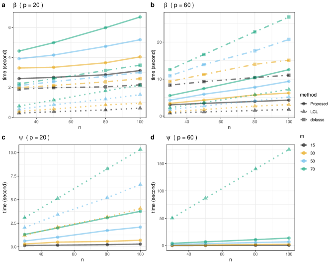
Figure 6: a and b: Computation time to estimate and infer the fixed effect coefficients $\beta$. c and d: Computation time to estimate the variance components.

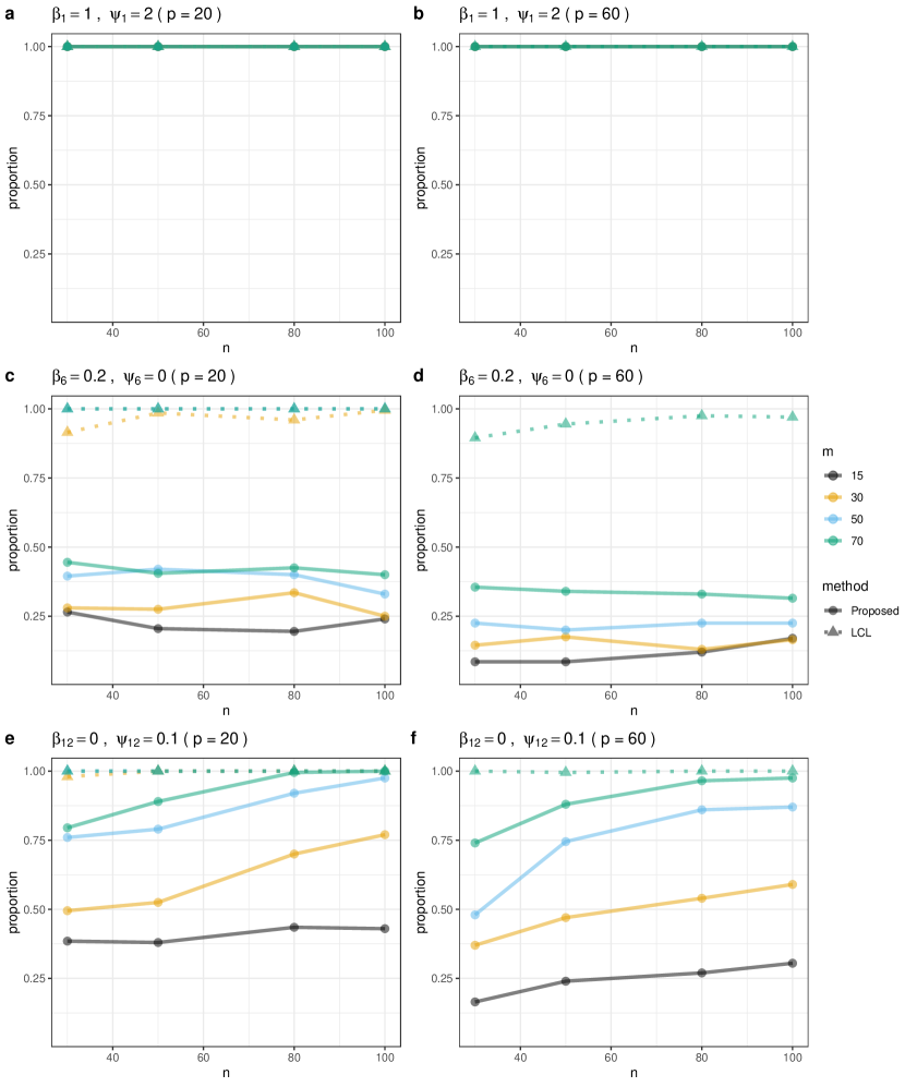
Figure 7: Proportion of 200 Monte Carlo simulations that provide non-zero estimate for the selected variance component. The title of each subplot shows the true values of the targeted fixed effect coefficient $\beta_{j}$, the corresponding random effect variance component $\psi_{j}$, and the value of $p$ in the setting. LCL does not estimate variance components when $m<q$, and thus for those $m$ the results for LCL are missing.

Table 2: Type-I error for testing zero $\beta_{l}$’s at 0.05 significance level under the simulation settings in the main paper. Bold face highlights type-I errors exceeding the normal range considering a Monte Carlo error of 0.03 with 200 replications.

			$\beta_{10}=0\ \psi_{10}=4$			$\beta_{11}=0\ \psi_{11}=0$			$\beta_{12}=0\ \psi_{12}=0.1$
p	m	n	Proposed	LCL	dblasso	Proposed	LCL	dblasso	Proposed	LCL	dblasso
		30	0.06	0.04	0.41	0.045	0.035	0.04	0.045	0.055	0.06
		50	0.05	0.04	0.44	0.04	0.03	0.035	0.045	0.045	0.09
		80	0.055	0.05	0.465	0.03	0.035	0.065	0.08	0.065	0.04
	15	100	0.035	0.055	0.445	0.04	0.065	0.04	0.04	0.03	0.06
		30	0.04	0.04	0.535	0.035	0.08	0.065	0.035	0.095	0.07
		50	0.03	0.01	0.525	0.055	0.075	0.065	0.07	0.085	0.055
		80	0.03	0.055	0.57	0.03	0.08	0.05	0.03	0.035	0.075
	30	100	0.06	0.055	0.525	0.06	0.07	0.05	0.035	0.06	0.08
		30	0.075	0.085	0.695	0.07	0.17	0.035	0.05	0.125	0.125
		50	0.05	0.085	0.655	0.06	0.16	0.07	0.06	0.11	0.08
		80	0.04	0.04	0.67	0.055	0.115	0.065	0.03	0.075	0.105
	50	100	0.04	0.06	0.65	0.03	0.155	0.075	0.055	0.125	0.125
		30	0.06	0.06	0.74	0.055	0.28	0.055	0.065	0.175	0.115
		50	0.055	0.07	0.72	0.035	0.225	0.05	0.045	0.135	0.105
		80	0.04	0.07	0.68	0.04	0.19	0.04	0.05	0.095	0.16
	70	100	0.065	0.055	0.71	0.055	0.22	0.045	0.055	0.075	0.125
		30	0.045	0.07	0.755	0.035	0.35	0.03	0.025	0.215	0.115
		50	0.031	0.066	0.74	0.041	0.311	0.066	0.087	0.199	0.173
		80	0.056	0.061	0.756	0.03	0.259	0.046	0.056	0.112	0.193
20	120	100	0.061	0.071	0.77	0.051	0.27	0.041	0.036	0.107	0.179
		30	0.08	0.075	0.425	0.035	0.045	0.045	0.05	0.045	0.065
		50	0.03	0.03	0.45	0.045	0.05	0.06	0.06	0.07	0.04
		80	0.035	0.045	0.465	0.065	0.055	0.06	0.04	0.045	0.05
	15	100	0.045	0.05	0.435	0.04	0.05	0.035	0.065	0.06	0.08
		30	0.09	0.1	0.525	0.03	0.04	0.03	0.07	0.065	0.105
		50	0.065	0.05	0.555	0.04	0.06	0.06	0.04	0.04	0.065
		80	0.055	0.055	0.585	0.035	0.045	0.045	0.045	0.045	0.07
	30	100	0.08	0.07	0.575	0.06	0.055	0.055	0.055	0.055	0.08
		30	0.02	0.03	0.705	0.035	0.065	0.035	0.07	0.065	0.075
		50	0.055	0.055	0.65	0.055	0.045	0.045	0.07	0.055	0.08
		80	0.055	0.075	0.665	0.045	0.05	0.07	0.04	0.025	0.09
	50	100	0.09	0.075	0.64	0.07	0.05	0.05	0.03	0.035	0.085
		30	0.045	0.05	0.665	0.065	0.09	0.045	0.05	0.07	0.11
		50	0.06	0.055	0.68	0.065	0.09	0.035	0.035	0.04	0.08
		80	0.065	0.06	0.715	0.07	0.07	0.035	0.065	0.08	0.11
	70	100	0.065	0.06	0.61	0.065	0.045	0.045	0.025	0.03	0.095
		30	0.045	0.055	0.725	0.055	0.235	0.05	0.03	0.145	0.115
		50	0.06	0.06	0.744	0.04	0.216	0.05	0.06	0.156	0.181
		80	0.06	0.08	0.745	0.06	0.205	0.055	0.06	0.13	0.17
60	120	100	0.09	0.08	0.765	0.04	0.12	0.04	0.025	0.085	0.145

Table 3: Confidence interval coverage for the $\beta_{l}$’s under the simulation settings in the main paper. Bold face highlights type-I errors exceeding the normal range considering a Monte Carlo error of 0.03 with 200 replications.

			$\beta_{1}=1\ \psi_{1}=2$			$\beta_{2}=0.5\ \psi_{2}=0$			$\beta_{6}=0.2\ \psi_{6}=0$			$\beta_{7}=0.1\ \psi_{7}=0.1$			$\beta_{9}=0.05\ \psi_{9}=0.1$			$\beta_{10}=0\ \psi_{10}=4$			$\beta_{11}=0\ \psi_{11}=0$			$\beta_{12}=0\ \psi_{12}=0.1$
p	m	n	Proposed	LCL	dblasso	Proposed	LCL	dblasso	Proposed	LCL	dblasso	Proposed	LCL	dblasso	Proposed	LCL	dblasso	Proposed	LCL	dblasso	Proposed	LCL	dblasso	Proposed	LCL	dblasso
		30	0.945	0.945	0.72	0.92	0.955	0.935	0.92	0.915	0.96	0.935	0.935	0.91	0.925	0.95	0.915	0.94	0.96	0.59	0.955	0.965	0.96	0.955	0.945	0.94
		50	0.94	0.94	0.725	0.925	0.945	0.985	0.935	0.96	0.915	0.94	0.945	0.965	0.935	0.93	0.925	0.95	0.96	0.56	0.96	0.97	0.965	0.955	0.955	0.91
		80	0.925	0.96	0.755	0.945	0.93	0.92	0.93	0.95	0.96	0.925	0.965	0.965	0.965	0.95	0.935	0.945	0.95	0.535	0.97	0.965	0.935	0.92	0.935	0.96
	15	100	0.965	0.965	0.78	0.945	0.94	0.96	0.975	0.965	0.97	0.945	0.96	0.935	0.93	0.94	0.925	0.965	0.945	0.555	0.96	0.935	0.96	0.96	0.97	0.94
		30	0.93	0.915	0.605	0.985	0.94	0.955	0.98	0.905	0.965	0.935	0.91	0.955	0.945	0.875	0.92	0.96	0.96	0.465	0.965	0.92	0.935	0.965	0.905	0.93
		50	0.945	0.925	0.605	0.975	0.955	0.94	0.945	0.96	0.94	0.94	0.915	0.9	0.93	0.89	0.915	0.97	0.99	0.475	0.945	0.925	0.935	0.93	0.915	0.945
		80	0.95	0.94	0.545	0.975	0.95	0.95	0.975	0.945	0.915	0.94	0.935	0.92	0.965	0.915	0.92	0.97	0.945	0.43	0.97	0.92	0.95	0.97	0.965	0.925
	30	100	0.935	0.935	0.57	0.98	0.96	0.945	0.94	0.915	0.95	0.965	0.92	0.935	0.93	0.91	0.935	0.94	0.945	0.475	0.94	0.93	0.95	0.965	0.94	0.92
		30	0.915	0.9	0.49	0.985	0.89	0.98	0.99	0.87	0.98	0.93	0.82	0.925	0.94	0.85	0.895	0.925	0.915	0.305	0.93	0.83	0.965	0.95	0.875	0.875
		50	0.925	0.92	0.505	0.985	0.935	0.95	0.975	0.905	0.96	0.95	0.905	0.885	0.93	0.865	0.885	0.95	0.915	0.345	0.94	0.84	0.93	0.94	0.89	0.92
		80	0.945	0.935	0.54	0.99	0.92	0.965	0.985	0.92	0.94	0.965	0.92	0.92	0.93	0.91	0.935	0.96	0.96	0.33	0.945	0.885	0.935	0.97	0.925	0.895
	50	100	0.95	0.945	0.475	0.94	0.925	0.955	0.945	0.88	0.94	0.97	0.925	0.905	0.95	0.92	0.905	0.96	0.94	0.35	0.97	0.845	0.925	0.945	0.875	0.875
		30	0.95	0.91	0.43	0.985	0.905	0.965	1	0.86	0.975	0.94	0.86	0.88	0.94	0.81	0.845	0.94	0.94	0.26	0.945	0.72	0.945	0.935	0.825	0.885
		50	0.955	0.92	0.345	0.995	0.92	0.93	0.995	0.88	0.96	0.92	0.89	0.885	0.97	0.91	0.895	0.945	0.93	0.28	0.965	0.775	0.95	0.955	0.865	0.895
		80	0.955	0.93	0.46	0.985	0.945	0.965	0.99	0.915	0.95	0.975	0.945	0.925	0.965	0.94	0.92	0.96	0.93	0.32	0.96	0.81	0.96	0.95	0.905	0.84
	70	100	0.97	0.965	0.5	0.995	0.93	0.93	0.975	0.94	0.94	0.915	0.885	0.86	0.945	0.905	0.895	0.935	0.945	0.29	0.945	0.78	0.955	0.945	0.925	0.875
		30	0.97	0.955	0.305	1	0.91	0.93	1	0.8	0.92	0.98	0.835	0.86	0.96	0.76	0.81	0.955	0.93	0.245	0.965	0.65	0.97	0.975	0.785	0.885
		50	0.959	0.923	0.372	0.995	0.878	0.949	1	0.852	0.939	0.959	0.852	0.842	0.959	0.878	0.842	0.969	0.934	0.26	0.959	0.689	0.934	0.913	0.801	0.827
		80	0.924	0.924	0.325	0.99	0.888	0.964	0.995	0.868	0.949	0.98	0.909	0.843	0.964	0.909	0.868	0.944	0.939	0.244	0.97	0.741	0.954	0.944	0.888	0.807
20	120	100	0.923	0.934	0.281	1	0.872	0.929	0.995	0.913	0.934	0.959	0.918	0.847	0.923	0.908	0.842	0.939	0.929	0.23	0.949	0.73	0.959	0.964	0.893	0.821
		30	0.91	0.915	0.74	0.955	0.985	0.99	0.945	0.97	0.96	0.91	0.925	0.92	0.965	0.97	0.94	0.92	0.925	0.575	0.965	0.955	0.955	0.95	0.955	0.935
		50	0.945	0.965	0.77	0.93	0.96	0.96	0.93	0.93	0.945	0.925	0.94	0.945	0.95	0.94	0.91	0.97	0.97	0.55	0.955	0.95	0.94	0.94	0.93	0.96
		80	0.94	0.93	0.735	0.93	0.95	0.975	0.97	0.97	0.965	0.945	0.965	0.945	0.955	0.945	0.955	0.965	0.955	0.535	0.935	0.945	0.94	0.96	0.955	0.95
	15	100	0.96	0.955	0.78	0.975	0.955	0.99	0.95	0.955	0.925	0.955	0.92	0.97	0.94	0.945	0.95	0.955	0.95	0.565	0.96	0.95	0.965	0.935	0.94	0.92
		30	0.94	0.93	0.705	0.94	0.965	0.94	0.925	0.94	0.94	0.945	0.935	0.965	0.945	0.945	0.915	0.91	0.9	0.475	0.97	0.96	0.97	0.93	0.935	0.895
		50	0.945	0.945	0.625	0.93	0.96	0.95	0.945	0.97	0.935	0.96	0.935	0.945	0.975	0.98	0.945	0.935	0.95	0.445	0.96	0.94	0.94	0.96	0.96	0.935
		80	0.945	0.955	0.63	0.95	0.95	0.935	0.98	0.975	0.975	0.96	0.965	0.96	0.955	0.945	0.95	0.945	0.945	0.415	0.965	0.955	0.955	0.955	0.955	0.93
	30	100	0.965	0.96	0.66	0.95	0.97	0.945	0.94	0.94	0.92	0.94	0.95	0.94	0.94	0.965	0.975	0.92	0.93	0.425	0.94	0.945	0.945	0.945	0.945	0.92
		30	0.945	0.955	0.52	0.945	0.975	0.945	0.94	0.965	0.96	0.96	0.97	0.935	0.955	0.95	0.875	0.98	0.97	0.295	0.965	0.935	0.965	0.93	0.935	0.925
		50	0.91	0.935	0.495	0.955	0.965	0.96	0.95	0.97	0.95	0.95	0.91	0.93	0.935	0.95	0.92	0.945	0.945	0.35	0.945	0.955	0.955	0.93	0.945	0.92
		80	0.955	0.945	0.535	0.98	0.985	0.96	0.955	0.99	0.955	0.935	0.96	0.94	0.94	0.945	0.93	0.945	0.925	0.335	0.955	0.95	0.93	0.96	0.975	0.91
	50	100	0.915	0.925	0.525	0.94	0.96	0.925	0.965	0.965	0.94	0.94	0.935	0.95	0.94	0.965	0.9	0.91	0.925	0.36	0.93	0.95	0.95	0.97	0.965	0.915
		30	0.94	0.925	0.51	0.975	0.98	0.955	0.965	0.96	0.955	0.95	0.94	0.915	0.995	0.96	0.92	0.955	0.95	0.335	0.935	0.91	0.955	0.95	0.93	0.89
		50	0.975	0.97	0.535	0.95	0.965	0.925	0.975	0.955	0.96	0.945	0.935	0.895	0.95	0.955	0.905	0.94	0.945	0.32	0.935	0.91	0.965	0.965	0.96	0.92
		80	0.945	0.96	0.455	0.955	0.965	0.94	0.955	0.94	0.975	0.96	0.93	0.875	0.935	0.93	0.9	0.935	0.94	0.285	0.93	0.93	0.965	0.935	0.92	0.89
	70	100	0.96	0.97	0.42	0.935	0.955	0.935	0.94	0.965	0.945	0.93	0.94	0.93	0.935	0.94	0.88	0.935	0.94	0.39	0.935	0.955	0.955	0.975	0.97	0.905
		30	0.935	0.935	0.365	0.995	0.91	0.945	0.995	0.83	0.94	0.935	0.87	0.89	0.895	0.82	0.89	0.955	0.945	0.275	0.945	0.765	0.95	0.97	0.855	0.885
		50	0.945	0.915	0.407	0.995	0.935	0.915	0.98	0.884	0.905	0.935	0.894	0.894	0.97	0.92	0.874	0.94	0.94	0.256	0.96	0.784	0.95	0.94	0.844	0.819
		80	0.95	0.955	0.395	0.995	0.935	0.92	0.985	0.935	0.935	0.975	0.935	0.885	0.935	0.9	0.87	0.94	0.92	0.255	0.94	0.795	0.945	0.94	0.87	0.83
60	120	100	0.945	0.96	0.345	0.99	0.985	0.925	0.995	0.96	0.94	0.945	0.935	0.9	0.96	0.9	0.885	0.91	0.92	0.235	0.96	0.88	0.96	0.975	0.915	0.855

Table 4: Power for testing non-zero $\beta_{l}$’s under the simulation settings in the main paper.

			$\beta_{1}=1\ \psi_{1}=2$		$\beta_{2}=0.5\ \psi_{2}=0$		$\beta_{6}=0.2\ \psi_{6}=0$		$\beta_{7}=0.1\ \psi_{7}=0.1$		$\beta_{9}=0.05\ \psi_{9}=0.1$
p	m	n	Proposed	LCL	Proposed	LCL	Proposed	LCL	Proposed	LCL	Proposed	LCL
		30	0.865	0.950	0.975	0.975	0.380	0.340	0.105	0.130	0.090	0.065
		50	0.975	1.000	1.000	1.000	0.700	0.620	0.145	0.170	0.085	0.085
		80	0.995	1.000	1.000	1.000	0.825	0.820	0.275	0.330	0.065	0.065
	15	100	1.000	1.000	1.000	1.000	0.870	0.880	0.290	0.305	0.145	0.115
		30	0.920	0.935	1.000	0.945	0.965	0.820	0.250	0.270	0.105	0.170
		50	1.000	0.995	1.000	0.995	0.995	0.955	0.340	0.360	0.120	0.155
		80	1.000	1.000	1.000	1.000	1.000	0.985	0.515	0.530	0.135	0.135
	30	100	1.000	1.000	1.000	1.000	1.000	0.985	0.635	0.640	0.160	0.175
		30	0.975	0.975	1.000	0.985	1.000	0.900	0.270	0.325	0.095	0.200
		50	1.000	0.990	1.000	0.985	1.000	0.955	0.485	0.440	0.125	0.220
		80	1.000	1.000	1.000	1.000	1.000	0.975	0.720	0.655	0.175	0.255
	50	100	1.000	1.000	1.000	1.000	1.000	0.985	0.805	0.770	0.250	0.285
		30	0.955	0.910	1.000	0.975	1.000	0.880	0.255	0.310	0.105	0.220
		50	0.995	0.995	1.000	0.995	1.000	0.955	0.475	0.470	0.155	0.205
		80	1.000	1.000	1.000	1.000	1.000	0.990	0.720	0.680	0.210	0.290
	70	100	1.000	1.000	1.000	1.000	1.000	0.995	0.775	0.680	0.230	0.245
		30	0.995	0.975	1.000	0.985	1.000	0.925	0.315	0.380	0.120	0.235
		50	0.995	0.995	1.000	0.980	1.000	0.944	0.531	0.500	0.133	0.235
		80	1.000	1.000	1.000	0.995	1.000	0.995	0.761	0.711	0.223	0.259
20	120	100	1.000	1.000	1.000	0.995	1.000	0.985	0.862	0.735	0.250	0.311
		30	0.825	0.870	0.810	0.940	0.235	0.250	0.115	0.110	0.035	0.025
		50	0.990	1.000	0.930	0.990	0.405	0.410	0.115	0.110	0.100	0.090
		80	1.000	1.000	0.995	1.000	0.555	0.645	0.130	0.065	0.065	0.075
	15	100	1.000	1.000	1.000	1.000	0.645	0.690	0.080	0.065	0.120	0.130
		30	0.925	0.950	0.995	1.000	0.490	0.525	0.135	0.100	0.095	0.090
		50	0.985	0.995	1.000	1.000	0.750	0.790	0.125	0.100	0.045	0.060
		80	1.000	1.000	1.000	1.000	0.910	0.935	0.210	0.210	0.155	0.205
	30	100	1.000	1.000	1.000	1.000	0.950	0.965	0.200	0.230	0.090	0.145
		30	0.925	0.960	1.000	1.000	0.685	0.780	0.110	0.110	0.080	0.070
		50	0.990	1.000	1.000	1.000	0.905	0.970	0.180	0.195	0.100	0.125
		80	1.000	1.000	1.000	1.000	0.985	1.000	0.295	0.310	0.110	0.160
	50	100	1.000	1.000	1.000	1.000	1.000	1.000	0.275	0.370	0.160	0.155
		30	0.935	0.945	1.000	0.995	0.920	0.840	0.140	0.150	0.060	0.105
		50	1.000	1.000	1.000	0.995	0.995	0.955	0.285	0.290	0.120	0.140
		80	1.000	1.000	1.000	1.000	1.000	0.990	0.410	0.405	0.130	0.165
	70	100	1.000	1.000	1.000	1.000	1.000	0.995	0.520	0.455	0.210	0.255
		30	0.980	0.965	1.000	0.975	1.000	0.875	0.265	0.290	0.110	0.185
		50	0.995	1.000	1.000	0.995	1.000	0.970	0.482	0.492	0.146	0.146
		80	1.000	1.000	1.000	1.000	1.000	0.990	0.590	0.555	0.215	0.250
60	120	100	1.000	1.000	1.000	1.000	1.000	0.995	0.700	0.680	0.270	0.315

Table 5: Point estimation accuracy for $\beta$, $\psi$ and $\sigma_{e}^{2}$ under the simulation settings in the main paper.

			$\beta$ total RMSE			$\psi$ total RMSE		$\sigma_{e}^{2}$ RMSE
p	m	n	Proposed	LCL	dblasso	Proposed	LCL	Proposed	LCL
		30	0.342	0.510	0.242	0.506	-	0.858	-
		50	0.257	0.403	0.188	0.494	-	0.729	-
		80	0.221	0.356	0.159	0.379	-	0.696	-
	15	100	0.199	0.321	0.152	0.285	-	0.585	-
		30	0.396	0.570	0.173	0.208	0.157	0.381	0.014
		50	0.274	0.441	0.114	0.239	0.141	0.334	0.003
		80	0.216	0.363	0.100	0.189	0.074	0.324	0.002
	30	100	0.193	0.329	0.099	0.208	0.081	0.318	0.003
		30	0.364	0.557	0.113	0.202	0.217	0.263	0.004
		50	0.278	0.459	0.086	0.158	0.161	0.216	0.01
		80	0.224	0.386	0.077	0.117	0.081	0.135	0.001
	50	100	0.188	0.338	0.066	0.076	0.075	0.164	0.001
		30	0.397	0.595	0.105	0.250	0.227	0.143	0.002
		50	0.287	0.484	0.097	0.143	0.14	0.191	0.002
		80	0.202	0.373	0.064	0.113	0.109	0.091	0.004
	70	100	0.185	0.352	0.058	0.061	0.084	0.066	0.001
		30	0.389	0.577	0.077	0.137	0.201	0.061	0.002
		50	0.272	0.485	0.056	0.118	0.181	0.063	0.001
		80	0.204	0.368	0.044	0.058	0.08	0.033	0.002
20	120	100	0.189	0.361	0.048	0.120	0.125	0.040	0.001
		30	0.431	0.575	0.402	0.912	-	1.245	-
		50	0.333	0.464	0.309	0.553	-	0.914	-
		80	0.272	0.384	0.251	0.480	-	0.805	-
	15	100	0.246	0.345	0.224	0.367	-	0.711	-
		30	0.332	0.461	0.295	0.511	-	0.544	-
		50	0.245	0.358	0.216	0.370	-	0.463	-
		80	0.195	0.298	0.176	0.220	-	0.420	-
	30	100	0.189	0.281	0.164	0.224	-	0.421	-
		30	0.278	0.396	0.190	0.297	-	0.380	-
		50	0.226	0.337	0.181	0.161	-	0.361	-
		80	0.166	0.264	0.137	0.176	-	0.268	-
	50	100	0.167	0.253	0.127	0.194	-	0.260	-
		30	0.329	0.487	0.173	0.166	0.203	0.249	0.002
		50	0.264	0.393	0.146	0.164	0.081	0.203	0.006
		80	0.195	0.323	0.123	0.124	0.089	0.160	0
	70	100	0.187	0.296	0.121	0.103	0.048	0.156	0.007
		30	0.361	0.568	0.130	0.164	0.211	0.133	0.005
		50	0.261	0.451	0.106	0.162	0.145	0.111	0.001
		80	0.215	0.392	0.098	0.107	0.083	0.098	0.003
60	120	100	0.202	0.352	0.087	0.082	0.1	0.058	0.003

F.2 Main results, effect of $a$

As discussed in Section 3, the framework works with any constant $a>0$. We treated $a$ as a tuning parameter in the main paper and used cross-validation to select $a$ in the main simulation study. In this section, we fix $a$ at a constant value for $a\in\{0.01,1,10,50\}$ and investigate the effect of $a$ on the finite sample performance of the proposed method. The rest of the simulation settings are the same as those in the main paper.

We illustrate the performance of the proposed method for $m=30$ in Figure 8 and Figure 9. We find that regardless of the value of the constant $a>0$, the proposed method can provide correct confidence interval coverage and control type-I error (Figure 8a,b,c,d). However, different choices of $a$ may impact the power of detecting non-zero $\beta_{l}$’s (Figure 8e,f), and the estimation accuracy of $\beta$ and the variance components (Figure 9).

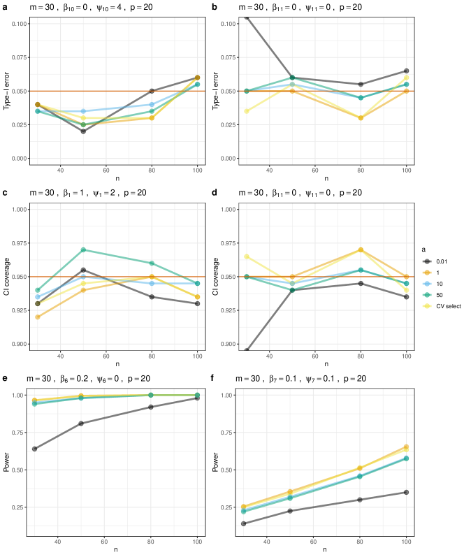
Figure 8: Simulation results for the proposed method with different values of $a$, where “$a=\text{CV select}$” corresponds to using cross-validation to choose $a$ for the proposed method. a,b: Type-I error for testing $\beta_{l}$’s at the 0.05 significance level (0.05 marked by red solid line). c,d: 95% confidence interval coverage (0.95 marked by red solid line) for fixed effect coefficients. e,f: Power for testing fixed effect coefficients at the 0.05 significance level. All results are computed for $p=20$ and $m=30$ based on 200 Monte Carlo simulations, and are plotted separately for each value of $a$, and against increasing $n$. The title of each subplot shows the true values of the targeted fixed effect coefficient $\beta_{l}$, and the corresponding random effect variance component $\psi_{l}$.

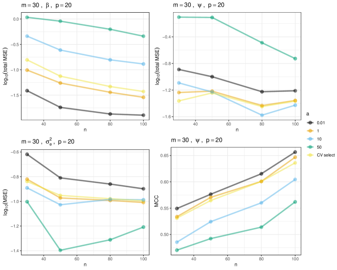
Figure 9: Simulation results for the proposed method with different values of $a$, where “$a=\text{CV select}$” corresponds to using cross-validation to choose $a$ for the proposed method. a: Total MSE on the $\log_{10}$ scale for estimating the fixed effect coefficients $\beta$. b: MSE on the $\log_{10}$ scale for estimating the noise variance $\sigma^{2}_{e}$. c: Total MSE on the $\log_{10}$ scale for estimating the random effect variance components $\psi$. d: Average MCC for identifying non-zero variance components, where we use non-zero estimates to select non-zero variance components. Values are computed for $p=20$ and $m=30$ based on 200 Monte Carlo simulations, are plotted separately for each $a$, and are against increasing $n$.

Appendix G Extension to High-Dimensional Heterogeneous VAR models

G.1 Simulation Study

G.1.1 Simulation Settings

We conduct simulation studies to compare the proposed estimator and inference procedures (referred to as MEVAR) with the standard lasso approach (Zhang and Zhang (2014), referred to as db-lasso). The standard lasso approach ignores the correlations among the observations. We compare the performance in terms of VAR coefficient estimation mean squared error (MSE), 95% confidence interval coverage, type-I error of testing zero coefficients and power of testing non-zero coefficients at 5% significance level.

We simulated data from the MEVAR(1) model (9) in the main paper. We reiterate the model formula below:

$$Y^{i}(t)=(\Phi+\Gamma^{i})Y^{i}(t-1)+\epsilon^{i}(t),$$

with $\Phi\in\mathop{\mathbb{R}}^{p\times p}$, $\mathop{\mathrm{vec}}(\Gamma^{i})\sim\mathop{\mathrm{N}}(0,\Sigma_{\Gamma})$, and $\epsilon^{i}(t)\sim\mathop{\mathrm{N}}(0,\Sigma_{\epsilon})$. We generated diagonal covariance matrices $\Sigma_{\Gamma}=\mathop{\mathrm{diag}}(\sigma_{\Gamma}^{2})$ and $\Sigma_{\epsilon}=\mathop{\mathrm{diag}}(\sigma_{\epsilon}^{2})$. The length $p^{2}$ vector $\sigma_{\Gamma}^{2}$ was sparse with each entry having a 0.1 probability of being non-zero, and the non-zero values were generated independently from $\mathrm{Unif}(0.05,0.15)$. The length $p$ vector $\sigma_{\epsilon}^{2}$ had a constant value of 0.5 for all entries. We generated a sparse group-level coefficient matrix $\Phi$, with each entry generated independently. The diagonal entries of $\Phi$ were generated from $\mathrm{Unif}(0.2,0.8)$; the off-diagonal entries were generated from a mixture distribution: each off-diagonal entry had a 0.8 probability of taking value 0, and had a 0.2 probability of following $N(0,0.04)$. We set $p=30$, $n\in\{20,40,60,80\}$, and $T\in\{25,50,100,150\}$. For each combination of $(n,T)$, we replicated 200 independent Monte Carlo simulations.

We used the same procedure as in the main paper to select the tuning parameters, except we followed the cross-validation procedure in Safikhani and Shojaie (2022) for time-series observations. The results are presented based on the optimal values of the tuning parameters. We used the hdi R-package Dezeure et al. (2015a) to implement the db-lasso approach.

G.1.2 Simulation Results

Without loss of generality, we focus on comparing the results for the first row of the coefficient matrix $\Phi$. Figure 10 presents the performance of the inference procedures for selected coefficients. The confidence intervals constructed by the MEVAR approach have good coverage for all coefficients (Figure 10a,b). In addition, the MEVAR approach always controls the type-I error rate at the nominal level (Figure 10c,d), and maintains reasonable power for detecting non-zero coefficients (Figure 10e,f). The standard db-lasso approach has inflated type-I error as high as 0.36, and poor confidence interval coverage as low as 0.19 for some of the coefficients (Figure 10a,d). We noticed that for those coefficients with the corresponding random effect variance being non-zero, i.e., when there is subject-level heterogeneity in the specific connection, the standard db-lasso would fail drastically. While for those coefficients that are fixed across subjects, the proposed MEVAR approach and the db-lasso approach provide similar results.

In terms of estimation, the proposed MEVAR approach consistently estimates the VAR coefficients with decreasing total MSE (Figure 11), even though its total MSE is slightly higher than the MSE yielded by the db-lasso approach.

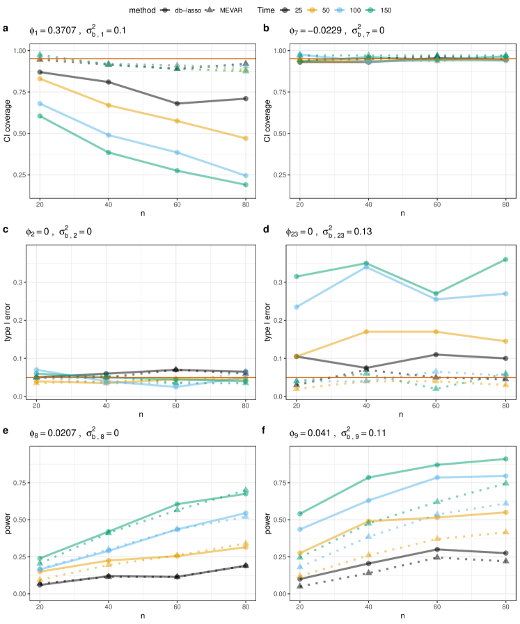
Figure 10: The performance of the inference procedures by MEVAR and db-lasso under different values of $n$ and $T$. a,b: the 95% confidence interval coverage for each coefficient (0.95 marked by red solid line); c,d: the type-I error of testing the zero coefficient at 5% significance level (0.05 marked by red solid line); e,f: the power of testing the non-zero coefficient at 5% significance level. The title of each subplot indicates the true value of the selected coefficient $\phi_{j}$ and its corresponding random effect variance $\sigma_{b,j}^{2}$.

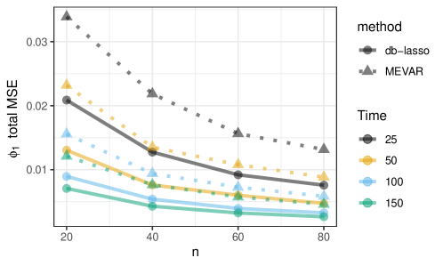
Figure 11: The total MSE of estimating the first row of $\Phi$, for the MEVAR approach and the db-lasso approach.

G.2 Theoretical Results

Without loss of generality, we establish the results for the first row of the matrix $\Phi$. For notational convenience, we omit the subscripts when the reference to quantities related to the first row of $\Phi$ is clear. Denote the first row of $\Phi$ by $\phi$. We can rewrite the model (10) for inferring $\phi$ as:

$$Y^{i}=X^{i}\phi+X^{i}\gamma^{i}+\epsilon^{i},\quad i=1,\dots,n,$$ (21)

where $Y^{i}$, $X^{i}$, $\gamma^{i}$ are sub-matrices/sub-vectors of $\tilde{Y}^{i}$, $\tilde{X}^{i}$ and $\mathop{\mathrm{vec}}(\Gamma^{i})$ that corresponds to inferring $\phi$. Here, $\gamma^{i}\sim\mathop{\mathrm{N}}(0,\Sigma_{\gamma})$ and $\epsilon^{i}\sim\mathop{\mathrm{N}}(0,\Sigma_{e})$, with $\Sigma_{\gamma}=\mathop{\mathrm{diag}}(\sigma_{\Gamma,1:p}^{2})$ and $\Sigma_{e}=\mathop{\mathrm{diag}}(\sigma^{2}_{\epsilon,1:p})$. We allow for either $p>c_{0}T$ or $T>c_{0}p$ for some constant $c_{0}>1$.

We first state the pivotal lemma that connects the singular values of $X^{i}$ to the singular values of a standard Gaussian matrix. Suppose $\sigma(X)$ denotes a non-zero singular value of the matrix $X$. We write $A\prec B$ if $B-A$ is a positive semi-definite matrix.

Lemma 20.

Suppose $X\in\mathop{\mathbb{R}}^{T\times p}$ ($T\neq p$) is a Gaussian matrix with $\mathop{\mathrm{vec}}(X)\sim\mathop{\mathrm{N}}(0,\Xi)$. Define $Z\in\mathop{\mathbb{R}}^{T\times p}$ such that $\mathop{\mathrm{vec}}(Z)=\left(\Xi\right)^{-1/2}\mathop{\mathrm{vec}}(X)\sim\mathop{\mathrm{N}}(0,I_{Tp})$. We have that

$$\sqrt{\sigma_{\min}(\Xi)}\sigma_{\min}(Z)\leq\sigma(X)\leq\sqrt{\sigma_{\max}(\Xi)}\sigma_{\max}(Z).$$

We also have

$$X^{\top}(aXX^{\top}+I)^{-1}X\succ\sigma_{\min}(\Xi)Z^{\top}(a\sigma_{\max}(\Xi)ZZ^{\top}+I)^{-1}Z$$

$$X^{\top}(aXX^{\top}+I)^{-1}X\prec\sigma_{\max}(\Xi)Z^{\top}(a\sigma_{\min}(\Xi)ZZ^{\top}+I)^{-1}Z.$$

Then in order to make the proposed doubly high-dimensional LMM framework work for the MEVAR(1) case, a sufficient condition is $\sigma(\Xi^{i})\asymp 1$ where $\Xi^{i}=\mathop{\mathrm{Var}}(X^{i})$. This is in fact a mild condition under the following assumption:

Assumption 12.

For the $i$th subject, conditioning on $\Gamma^{i}$, the observations $\{Y^{i}(t)\}_{t=1}^{T}$ are realizations of a stationary Gaussian process.

Under Assumption 12, Proposition 2.3 of Basu and Michailidis (2015) bounds $\sigma(\Xi^{i})$ by the extreme eigenvalues of the matrix-valued spectral density function over the unit circle. According to Lemma 5.5 of Zheng and Raskutti (2019), we have $\sigma(\Xi^{i})\asymp 1$ when $\|\Phi+\Gamma^{i}\|_{2}\leq 1-\Delta$ holds for some $\Delta\in(0,1)$, which is a common condition for VAR process Zheng and Raskutti (2019); Neykov et al. (2018).

The rest of the proof directly follows the proof for inferring the fixed effect coefficients in a standard doubly high-dimensional LMM.

References

• Aulchenko et al. (2007) Y. S. Aulchenko, D.-J. De Koning, and C. Haley. Genomewide rapid association using mixed model and regression: a fast and simple method for genomewide pedigree-based quantitative trait loci association analysis. Genetics, 177(1):577–585, 2007.
• Basu and Michailidis (2015) S. Basu and G. Michailidis. Regularized estimation in sparse high-dimensional time series models. The Annals of Statistics, 43(4):1535–1567, 2015.
• Bhatia (2007) R. Bhatia. Perturbation bounds for matrix eigenvalues. SIAM, 2007.
• Bradic et al. (2020) J. Bradic, G. Claeskens, and T. Gueuning. Fixed effects testing in high-dimensional linear mixed models. Journal of the American Statistical Association, 115(532):1835–1850, 2020.
• Bresler (2015) G. Bresler. Efficiently learning ising models on arbitrary graphs. In Proceedings of the forty-seventh annual ACM symposium on Theory of computing, pages 771–782, 2015.
• Brose et al. (2015) A. Brose, F. Schmiedek, P. Koval, and P. Kuppens. Emotional inertia contributes to depressive symptoms beyond perseverative thinking. Cognition and Emotion, 29(3):527–538, 2015.
• Bühlmann and Van De Geer (2011) P. Bühlmann and S. Van De Geer. Statistics for high-dimensional data: methods, theory and applications. Springer Science & Business Media, 2011.
• Cai et al. (2011) T. Cai, W. Liu, and X. Luo. A constrained $\ell$1 minimization approach to sparse precision matrix estimation. Journal of the American Statistical Association, 106(494):594–607, 2011.
• Chen et al. (2011) G. Chen, D. R. Glen, Z. S. Saad, J. P. Hamilton, M. E. Thomason, I. H. Gotlib, and R. W. Cox. Vector autoregression, structural equation modeling, and their synthesis in neuroimaging data analysis. Computers in biology and medicine, 41(12):1142–1155, 2011.
• Chen et al. (2015) S. Chen, D. M. Witten, and A. Shojaie. Selection and estimation for mixed graphical models. Biometrika, 102(1):47–64, 2015.
• Chiang et al. (2017) S. Chiang, M. Guindani, H. J. Yeh, Z. Haneef, J. M. Stern, and M. Vannucci. Bayesian vector autoregressive model for multi-subject effective connectivity inference using multi-modal neuroimaging data. Human brain mapping, 38(3):1311–1332, 2017.
• Defazio and Caetano (2012) A. Defazio and T. Caetano. A convex formulation for learning scale-free networks via submodular relaxation. Advances in neural information processing systems, 25, 2012.
• Deshpande et al. (2009) G. Deshpande, S. LaConte, G. A. James, S. Peltier, and X. Hu. Multivariate granger causality analysis of fmri data. Human brain mapping, 30(4):1361–1373, 2009.
• Deshpande et al. (2011) G. Deshpande, P. Santhanam, and X. Hu. Instantaneous and causal connectivity in resting state brain networks derived from functional mri data. Neuroimage, 54(2):1043–1052, 2011.
• Dezeure et al. (2015a) R. Dezeure, P. Bühlmann, L. Meier, and N. Meinshausen. High-dimensional inference: confidence intervals, p-values and r-software hdi. Statistical science, pages 533–558, 2015a.
• Dezeure et al. (2015b) R. Dezeure, P. Bühlmann, L. Meier, and N. Meinshausen. High-dimensional inference: Confidence intervals, p-values and R-software hdi. Statistical Science, 30(4):533–558, 2015b.
• Dyrba et al. (2020) M. Dyrba, R. Mohammadi, M. J. Grothe, T. Kirste, and S. J. Teipel. Gaussian graphical models reveal inter-modal and inter-regional conditional dependencies of brain alterations in alzheimer’s disease. Frontiers in aging neuroscience, 12:99, 2020.
• Fan and Li (2012) Y. Fan and R. Li. Variable selection in linear mixed effects models. Annals of Statistics, 40(4):2043, 2012.
• Friedman et al. (2008) J. Friedman, T. Hastie, and R. Tibshirani. Sparse inverse covariance estimation with the graphical lasso. Biostatistics, 9(3):432–441, 2008.
• Friedman et al. (2010) J. Friedman, T. Hastie, and R. Tibshirani. Regularization paths for generalized linear models via coordinate descent. Journal of Statistical Software, 33(1):1–22, 2010. URL https://www.jstatsoft.org/v33/i01/.
• Friston (2011) K. J. Friston. Functional and effective connectivity: a review. Brain connectivity, 1(1):13–36, 2011.
• Glasser et al. (2013) M. F. Glasser, S. N. Sotiropoulos, J. A. Wilson, T. S. Coalson, B. Fischl, J. L. Andersson, J. Xu, S. Jbabdi, M. Webster, J. R. Polimeni, et al. The minimal preprocessing pipelines for the human connectome project. Neuroimage, 80:105–124, 2013.
• Gorrostieta et al. (2012) C. Gorrostieta, H. Ombao, P. Bédard, and J. N. Sanes. Investigating brain connectivity using mixed effects vector autoregressive models. NeuroImage, 59(4):3347–3355, 2012.
• Gorrostieta et al. (2013) C. Gorrostieta, M. Fiecas, H. Ombao, E. Burke, and S. Cramer. Hierarchical vector auto-regressive models and their applications to multi-subject effective connectivity. Frontiers in computational neuroscience, 7:159, 2013.
• Granger (1969) C. W. Granger. Investigating causal relations by econometric models and cross-spectral methods. Econometrica: journal of the Econometric Society, pages 424–438, 1969.
• Griffanti et al. (2014) L. Griffanti, G. Salimi-Khorshidi, C. F. Beckmann, E. J. Auerbach, G. Douaud, C. E. Sexton, E. Zsoldos, K. P. Ebmeier, N. Filippini, C. E. Mackay, et al. Ica-based artefact removal and accelerated fmri acquisition for improved resting state network imaging. Neuroimage, 95:232–247, 2014.
• Han et al. (2015) F. Han, H. Lu, and H. Liu. A direct estimation of high dimensional stationary vector autoregressions. Journal of Machine Learning Research, 2015.
• Heishman et al. (1997) S. J. Heishman, K. Arasteh, and M. L. Stitzer. Comparative effects of alcohol and marijuana on mood, memory, and performance. Pharmacology Biochemistry and Behavior, 58(1):93–101, 1997.
• Holm (1979) S. Holm. A simple sequentially rejective multiple test procedure. Scandinavian Journal of Statistics, pages 65–70, 1979.
• Janková and van de Geer (2017) J. Janková and S. van de Geer. Honest confidence regions and optimality in high-dimensional precision matrix estimation. Test, 26(1):143–162, 2017.
• Janková and van de Geer (2018) J. Janková and S. van de Geer. Inference in high-dimensional graphical models. arXiv preprint arXiv:1801.08512, 2018.
• Krumsiek et al. (2011) J. Krumsiek, K. Suhre, T. Illig, J. Adamski, and F. J. Theis. Gaussian graphical modeling reconstructs pathway reactions from high-throughput metabolomics data. BMC systems biology, 5(1):1–16, 2011.
• Lee et al. (2016) E.-S. Lee, K. Yoo, Y.-B. Lee, J. Chung, J.-E. Lim, B. Yoon, and Y. Jeong. Default mode network functional connectivity in early and late mild cognitive impairment. Alzheimer Disease & Associated Disorders, 30(4):289–296, 2016.
• Li et al. (2021) S. Li, T. T. Cai, and H. Li. Inference for high-dimensional linear mixed-effects models: A quasi-likelihood approach. Journal of the American Statistical Association, pages 1–33, 2021.
• Li et al. (2018) Y. Li, S. Wang, P. X.-K. Song, N. Wang, L. Zhou, and J. Zhu. Doubly regularized estimation and selection in linear mixed-effects models for high-dimensional longitudinal data. Statistics and its interface, 11(4):721, 2018.
• Lin et al. (2016) L. Lin, M. Drton, and A. Shojaie. Estimation of high-dimensional graphical models using regularized score matching. Electronic journal of statistics, 10(1):806, 2016.
• Lin et al. (2020) L. Lin, M. Drton, and A. Shojaie. Statistical significance in high-dimensional linear mixed models. In Proceedings of the 2020 ACM-IMS on Foundations of Data Science Conference, pages 171–181, 2020.
• Liu et al. (2012) H. Liu, F. Han, M. Yuan, J. Lafferty, and L. Wasserman. High-dimensional semiparametric gaussian copula graphical models. The Annals of Statistics, 40(4):2293–2326, 2012.
• Liu and Tiao (1980) L.-M. Liu and G. C. Tiao. Random coefficient first-order autoregressive models. Journal of Econometrics, 13(3):305–325, 1980.
• Liu (2013) W. Liu. Gaussian graphical model estimation with false discovery rate control. The Annals of Statistics, 41(6):2948–2978, 2013.
• Liu and Chen (2020) X. Liu and R. Chen. Threshold factor models for high-dimensional time series. Journal of Econometrics, 216(1):53–70, 2020.
• Matthews (1975) B. W. Matthews. Comparison of the predicted and observed secondary structure of t4 phage lysozyme. Biochimica et Biophysica Acta (BBA)-Protein Structure, 405(2):442–451, 1975.
• Meinshausen and Bühlmann (2006) N. Meinshausen and P. Bühlmann. High-dimensional graphs and variable selection with the lasso. The Annals of Statistics, 34(3):1436–1462, 2006.
• Monti et al. (2017) R. P. Monti, C. Anagnostopoulos, and G. Montana. Learning population and subject-specific brain connectivity networks via mixed neighborhood selection. The Annals of Applied Statistics, pages 2142–2164, 2017.
• Morgan et al. (2011) V. L. Morgan, B. P. Rogers, H. H. Sonmezturk, J. C. Gore, and B. Abou-Khalil. Cross hippocampal influence in mesial temporal lobe epilepsy measured with high temporal resolution functional magnetic resonance imaging. Epilepsia, 52(9):1741–1749, 2011.
• Mumford and Nichols (2006) J. A. Mumford and T. Nichols. Modeling and inference of multisubject fmri data. IEEE Engineering in Medicine and Biology Magazine, 25(2):42–51, 2006.
• Nandram and Petruccelli (1997) B. Nandram and J. D. Petruccelli. A bayesian analysis of autoregressive time series panel data. Journal of Business & Economic Statistics, 15(3):328–334, 1997.
• Narayan and Allen (2016) M. Narayan and G. I. Allen. Mixed effects models for resampled network statistics improves statistical power to find differences in multi-subject functional connectivity. Frontiers in neuroscience, 10:108, 2016.
• Neykov et al. (2018) M. Neykov, Y. Ning, J. S. Liu, and H. Liu. A Unified Theory of Confidence Regions and Testing for High-Dimensional Estimating Equations. Statistical Science, 33(3):427 – 443, 2018. doi: 10.1214/18-STS661. URL https://doi.org/10.1214/18-STS661.
• Ng et al. (2013) B. Ng, G. Varoquaux, J. B. Poline, and B. Thirion. A novel sparse group gaussian graphical model for functional connectivity estimation. In International Conference on Information Processing in Medical Imaging, pages 256–267. Springer, 2013.
• Nicholls and Quinn (1981) D. Nicholls and B. Quinn. The estimation of multivariate random coefficient autoregressive models. Journal of Multivariate Analysis, 11(4):544–555, 1981.
• Olszowy et al. (2019) W. Olszowy, J. Aston, C. Rua, and G. B. Williams. Accurate autocorrelation modeling substantially improves fmri reliability. Nature communications, 10(1):1220, 2019.
• Qiao et al. (2019) X. Qiao, S. Guo, and G. M. James. Functional graphical models. Journal of the American Statistical Association, 114(525):211–222, 2019.
• Ray et al. (2015) A. Ray, S. Sanghavi, and S. Shakkottai. Improved greedy algorithms for learning graphical models. IEEE Transactions on Information Theory, 61(6):3457–3468, 2015.
• Regis et al. (2022) M. Regis, P. Serra, and E. R. van den Heuvel. Random autoregressive models: A structured overview. Econometric Reviews, 41(2):207–230, 2022.
• Ren et al. (2015) Z. Ren, T. Sun, C.-H. Zhang, and H. H. Zhou. Asymptotic normality and optimalities in estimation of large gaussian graphical models. The Annals of Statistics, 43(3):991–1026, 2015.
• Safikhani and Shojaie (2022) A. Safikhani and A. Shojaie. Joint structural break detection and parameter estimation in high-dimensional nonstationary var models. Journal of the American Statistical Association, 117(537):251–264, 2022.
• Shojaie (2020) A. Shojaie. Differential network analysis: A statistical perspective. Wiley Interdisciplinary Reviews: Computational Statistics, 2020.
• Shojaie and Fox (2022) A. Shojaie and E. B. Fox. Granger causality: A review and recent advances. Annual Review of Statistics and Its Application, 9:289–319, 2022.
• Shojaie and Michailidis (2010) A. Shojaie and G. Michailidis. Discovering graphical granger causality using the truncating lasso penalty. Bioinformatics, 26(18):i517–i523, 2010.
• Smith et al. (2011) S. M. Smith, K. L. Miller, G. Salimi-Khorshidi, M. Webster, C. F. Beckmann, T. E. Nichols, J. D. Ramsey, and M. W. Woolrich. Network modelling methods for fmri. Neuroimage, 54(2):875–891, 2011.
• Smith et al. (2013) S. M. Smith, C. F. Beckmann, J. Andersson, E. J. Auerbach, J. Bijsterbosch, G. Douaud, E. Duff, D. A. Feinberg, L. Griffanti, M. P. Harms, et al. Resting-state fmri in the human connectome project. Neuroimage, 80:144–168, 2013.
• Smith et al. (2014) S. M. Smith, A. Hyvärinen, G. Varoquaux, K. L. Miller, and C. F. Beckmann. Group-pca for very large fmri datasets. Neuroimage, 101:738–749, 2014.
• Smith et al. (2015) S. M. Smith, T. E. Nichols, D. Vidaurre, A. M. Winkler, T. E. Behrens, M. F. Glasser, K. Ugurbil, D. M. Barch, D. C. Van Essen, and K. L. Miller. A positive-negative mode of population covariation links brain connectivity, demographics and behavior. Nature Neuroscience, 18(11):1565–1567, 2015.
• Sofer (2017) T. Sofer. Confidence intervals for heritability via haseman-elston regression. Statistical Applications in Genetics and Molecular Biology, 16(4):259–273, 2017.
• Solea and Li (2020) E. Solea and B. Li. Copula gaussian graphical models for functional data. Journal of the American Statistical Association, pages 1–13, 2020.
• Sporns (2007) O. Sporns. Brain connectivity. Scholarpedia, 2(10):4695, 2007. doi: 10.4249/scholarpedia.4695. revision #91084.
• Tank et al. (2021) A. Tank, X. Li, E. B. Fox, and A. Shojaie. The convex mixture distribution: Granger causality for categorical time series. SIAM Journal on Mathematics of Data Science, 3(1):83–112, 2021.
• Trench (1999) W. F. Trench. Asymptotic distribution of the spectra of a class of generalized kac–murdock–szegö matrices. Linear algebra and its applications, 294(1-3):181–192, 1999.
• Tropp (2015) J. A. Tropp. An introduction to matrix concentration inequalities. arXiv preprint arXiv:1501.01571, 2015.
• Van Essen et al. (2013) D. C. Van Essen, S. M. Smith, D. M. Barch, T. E. Behrens, E. Yacoub, K. Ugurbil, W.-M. H. Consortium, et al. The wu-minn human connectome project: an overview. Neuroimage, 80:62–79, 2013.
• Vaněček (2008) P. Vaněček. Estimators of random coefficient autoregressive models. 2008.
• Voorman et al. (2014) A. Voorman, A. Shojaie, and D. Witten. Graph estimation with joint additive models. Biometrika, 101(1):85–101, 2014.
• Wang et al. (2012) L. P. Wang, E. Hamaker, and C. Bergeman. Investigating inter-individual differences in short-term intra-individual variability. Psychological methods, 17(4):567, 2012.
• Wang (2013) W. Wang. Identifiability of linear mixed effects models. Electronic Journal of Statistics, 7:244–263, 2013.
• Wang and Ip (2008) Y. J. Wang and E. H. Ip. Conditionally specified continuous distributions. Biometrika, 95(3):735–746, 2008.
• Whitfield-Gabrieli and Ford (2012) S. Whitfield-Gabrieli and J. M. Ford. Default mode network activity and connectivity in psychopathology. Annual review of clinical psychology, 8:49–76, 2012.
• Woolrich et al. (2001) M. W. Woolrich, B. D. Ripley, M. Brady, and S. M. Smith. Temporal autocorrelation in univariate linear modeling of fmri data. Neuroimage, 14(6):1370–1386, 2001.
• Yu et al. (2018) M. Yu, K. A. Linn, P. A. Cook, M. L. Phillips, M. McInnis, M. Fava, M. H. Trivedi, M. M. Weissman, R. T. Shinohara, and Y. I. Sheline. Statistical harmonization corrects site effects in functional connectivity measurements from multi-site fmri data. Human brain mapping, 39(11):4213–4227, 2018.
• Yu et al. (2019) S. Yu, M. Drton, and A. Shojaie. Generalized score matching for non-negative data. The Journal of Machine Learning Research, 20(1):2779–2848, 2019.
• Yuan and Lin (2007) M. Yuan and Y. Lin. Model selection and estimation in the gaussian graphical model. Biometrika, 94(1):19–35, 2007.
• Zhang and Zhang (2014) C.-H. Zhang and S. S. Zhang. Confidence intervals for low dimensional parameters in high dimensional linear models. Journal of the Royal Statistical Society: Series B (Statistical Methodology), 76(1):217–242, 2014.
• Zhang et al. (2022) K. Zhang, A. Safikhani, A. Tank, and A. Shojaie. Penalized estimation of threshold auto-regressive models with many components and thresholds. Electronic Journal of Statistics, 16(1):1891–1951, 2022.
• Zhang et al. (2020) Y. Zhang, G. Parmigiani, and W. E. Johnson. Combat-seq: batch effect adjustment for rna-seq count data. NAR genomics and bioinformatics, 2(3):lqaa078, 2020.
• Zhao and Duan (2019) H. Zhao and Z.-H. Duan. Cancer genetic network inference using gaussian graphical models. Bioinformatics and biology insights, 13:1177932219839402, 2019.
• Zhao et al. (2023) W. Zhao, C. Makowski, D. J. Hagler, H. P. Garavan, W. K. Thompson, D. J. Greene, T. L. Jernigan, and A. M. Dale. Task fmri paradigms may capture more behaviorally relevant information than resting-state functional connectivity. Neuroimage, 270:119946, 2023.
• Zheng and Raskutti (2019) L. Zheng and G. Raskutti. Testing for high-dimensional network parameters in auto-regressive models. Electronic Journal of Statistics, 13(2):4977–5043, 2019.