GET: Unlocking the Multi-modal Potential of CLIP for Generalized Category Discovery

Abstract

Given unlabelled datasets containing both old and new categories, generalized category discovery (GCD) aims to accurately discover new classes while correctly classifying old classes, leveraging the class concepts learned from labeled samples. Current GCD methods only use a single visual modality of information, resulting in poor classification of visually similar classes. Though certain classes are visually confused, their text information might be distinct, motivating us to introduce text information into the GCD task. However, the lack of class names for unlabelled data makes it impractical to utilize text information. To tackle this challenging problem, in this paper, we propose a Text Embedding Synthesizer (TES) to generate pseudo text embeddings for unlabelled samples. Specifically, our TES leverages the property that CLIP can generate aligned vision-language features, converting visual embeddings into tokens of the CLIP’s text encoder to generate pseudo text embeddings. Besides, we employ a dual-branch framework, through the joint learning and instance consistency of different modality branches, visual and semantic information mutually enhance each other, promoting the interaction and fusion of visual and text embedding space. Our method unlocks the multi-modal potentials of CLIP and outperforms the baseline methods by a large margin on all GCD benchmarks, achieving new state-of-the-art. The code will be released at https://github.com/enguangW/GET.

1 Introduction

Deep neural networks trained on large amounts of labeled data have shown powerful visual recognition capabilities [21], while this is heartening, the close-set assumption severely hinder the deployment of the model in practical application scenarios. Recently, novel class discovery (NCD) [14] has been proposed to categorize unknown classes of unlabelled data, leveraging the knowledge learned from labeled data. As a realistic extension to NCD, generalized category discovery (GCD) [36] assumes that the unlabelled data comes from both known and unknown classes, rather than just unknown classes as in NCD. The model needs to accurately discover unknown classes while correctly classifying known classes of the unlabelled data, breaking the close-set limitation, making GCD a challenging and meaningful task.

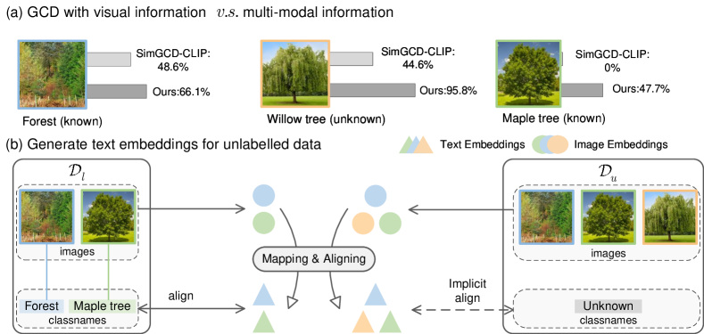
Figure 1: The motivation of our method. (a) Current GCD methods [40] rely on single visual features, resulting in poor classification of visually similar classes; Our approach introduces text information, improving the discriminative capabilities of the model. (b) Our proposed method maps image embeddings to text embeddings while simultaneously achieving modal alignment.

Previous GCD methods [36, 40, 43, 30, 45] utilize a DINO [4] pre-trained ViT as the backbone network to expect good initial discrimination ability of the model, thereby facilitating fine-tuning on the training data. Although promising results have been achieved, the representation of the DINO pre-trained model focuses on specific aspects of the data, resulting in large differences in the clustering performance for different classes in the downstream dataset. To explore the impact of different types of pre-trained models on GCD clustering performance, we conduct an extensive empirical investigation in Sec. 5.4. A key observation is that various pre-trained models perform inferior on distinguishing certain classes, especially those with visually similar appearances, such as the classes in all fine-grained datasets and some super-class subsets of generic datasets. We argue that this is due to the reliance on single visual modality information. Current GCD methods only utilize a single visual modality of information, even visual features obtained by the powerful CLIP [32] visual backbone are still difficult to generalize certain visual concepts, leading to sub-optimal results (see in Fig. 1 (a)). An evident fact is that, even if certain classes are visually confused, their textual information might be different and more discriminative, motivating us to introduce text information into the GCD task.

As we all know, thanks to the cross-modal alignment training of very large-scale image-text pairs, CLIP shows strong zero-shot performance, demonstrates its powerful generalization ability of multi-modal joint embedding, and a wide range of fine-grained visual concepts can be well separated in the multi-modal embedding space. In order to utilize multi-modal joint embedding for GCD tasks, it is a natural idea to conduct joint clustering training with the visual embedding of images and the text embedding of the corresponding class names. However, the lack of class names for unlabelled data in GCD makes it impractical to use the text encoder, thus locking the multi-modal potential of CLIP.

To tackle this challenging problem, in this paper, we propose a generative-based method to GEnerate pseudo Text embeddings for unlabelled data, dubbed GET. In particular, we introduce a Text Embedding Synthesizer (TES) module based on the vision-language alignment property of CLIP, producing reliable and modality-aligned pseudo text features. As shown in Fig. 1 (b), TES learns a mapping that transforms image embeddings into text embeddings. Specifically, the TES module converts visual embeddings into tokens of the CLIP’s text encoder, eliminating the need for textual input. To ensure that generated pseudo text embeddings reside in the same text space as real text embeddings and maintain consistency, TES aligns them with the real text embeddings generated by corresponding class names for labeled data, thus leading to an implicit alignment for unlabelled data. Besides, TES simultaneously aligns the text embedding and the image embedding of the same instance, enforcing the consistency between language and vision while preventing overfitting to known classes. This training approach renders TES equivalent to a special finetuned CLIP text encoder on a specific dataset with only visual input. From another perspective, our TES can be considered as performing an image captioning task [28].

To fully leverage such aligned multi-modal features in the GCD task, we propose a dual-branch multi-modal joint training strategy with a cross-modal instance consistency objective. One branch focuses on visual information, while the other branch supplements it with text information. Through joint learning on the GCD task, visual and semantic information aspects mutually enhance each other. Furthermore, our cross-modal instance consistency objective enforces the instance have the same relationship in both visual and text modalities with anchors constructed by labeled instances, promoting the interaction and alignment of visual and text embedding space. With the supplementation of text embeddings generated by TES and an appropriate dual-branch training strategy, the multi-modal features correct the classification hyperplane, enhancing discriminative ability while reducing bias issues.

To summarize, our contributions are as follows: (i) Through extensive empirical research, we demonstrate that GCD methods are constrained by pre-trained backbone and the representation of a single visual modality makes current GCD methods have inferior clustering performance on many visually similar classes. (ii) To unlock the potential of CLIP, We propose a TES module converting visual embeddings into tokens of the CLIP’s text encoder to generate pseudo text embeddings for each sample. Besides, through the cross-modal instance consistency objective in our dual-branch framework, information of different modalities mutually enhances each other, producing more discriminative classification prototypes. (iii)Our method achieves state-of-the-art results on multiple benchmarks, extending GCD to a multi-modal paradigm.

2 Related Works

Novel Class Discovery.

Novel class discovery (NCD) can be traced back to KCL [16], where pairwise similarity generated by similarity prediction network guides clustering reconstruction, offering a constructive approach for transfer learning across tasks and domains. Early methods are based on two objectives: pretraining on labeled data and clustering on unlabelled data. RS [13] performs a self-supervised pretraining on both labeled and unlabelled data, alleviating the model’s bias towards known classes. Simultaneously, RS proposes knowledge transfer through rank statistics, which has been widely adopted in subsequent research. [44] proposes a two-branch learning framework with dual ranking statistics, exchanging information through mutual knowledge distillation, which is similar to our approach to some extent. Differently, our two branches focus on semantic and visual information, rather than local and global characteristics in [44]. In order to simplify NCD approaches, UNO [11] recommends optimizing the task with a unified cross-entropy loss using the multi-view SwAV [3] exchange prediction strategy, which sets a new NCD paradigm.

Generalized Category Discovery.

Recently, generalized category discovery (GCD) [36] extends NCD to a more realistic scenario, where unlabelled data comes from both known and unknown classes. GCD [36] employs a pre-trained vision transformer [9] to provide initial visual representations, fine-tuning the backbone through supervised and self-supervised contrastive learning on the labeled and the entire data. Once the model learns discriminative representations, semi-supervised k-means is used for classification by constraining the correct clustering of labeled samples. As an emerging and realistic topic, GCD gradually gaining attention. PromptCAL [43] propose a two-stage framework to tackle the class collision issue caused by false negatives while enhancing the adaptability of the model on downstream datasets. CLIP-GCD [29] mines text descriptions from a large text corpus to use the text encoder and simply concatenates visual and text features for classification. In contrast, our method focuses on the dataset itself, without introducing additional corpus. SimGCD [40] introduces a parametric classification approach, addressing the computational overhead of GCD clustering while achieving remarkable improvements. Specifically, SimGCD adds a classifier on top of GCD and jointly learns self-distillation and supervised training strategies. In this paper, we try to tackle GCD in a parametric [40] way. Unlike previous works [36, 40, 43, 30, 45] that solely relies on visual information, we employ CLIP to introduce multi-modal information into the task, and outperforms current uni-visual-modality GCD methods by a large margin.

Vision-Language Pre-training.

Vision-Language pre-training [10, 5] aims to train a large-scale model on extensive image-text data, which, through fine-tuning, can achieve strong performance on a range of downstream visual-language tasks. Some studies [24, 7, 25, 34, 23] achieve improved performance in various image-language tasks by modeling image-text interactions through a fusion approach. However, the need to encode all image-text pairs in the fusion approach makes the inference speed in image-text retrieval tasks slow. Consequently, some studies [32, 17] propose a separate encoding of images and texts, and project image and text embeddings into a joint embedding space through contrastive learning. CLIP [32] uses contrastive training on large-scale image-text pairs, minimizing the distance between corresponding images and texts while simultaneously maximizing the distance between non-corresponding pairs. The strong generalization capabilities and multi-modal properties of CLIP prompt us to introduce it to the GCD Task.

3 Preliminaries

3.1 Problem formulation

In the context of GCD, the training data $\mathcal{D}$ is divided into a labeled dataset $\mathcal{D}_{l}=\left\{(\boldsymbol{x}_{i}^{l},{y}_{i}^{l})\right\}_{i=1}^{N}\in\mathcal{X}\times\mathcal{Y}_{l}$ and an unlabelled dataset $\mathcal{D}_{u}=\left\{(\boldsymbol{x}_{i}^{u},{y}_{i}^{u})\right\}_{i=1}^{M}\in\mathcal{X}\times\mathcal{Y}_{u}$, where $\mathcal{Y}_{l}$ and $\mathcal{Y}_{u}$ represent the label space while $\mathcal{Y}_{l}\subset\mathcal{Y}_{u}$, and $\mathcal{D}=\mathcal{D}_{l}\cup\mathcal{D}_{u}$. $|\mathcal{Y}_{l}|$ and $|\mathcal{Y}_{u}|$ represent the number of categories for labeled samples and unlabelled samples, respectively. The goal of GCD is to correctly cluster unlabelled samples with the help of labeled samples.

3.2 Parametric GCD method (SimGCD)

In this paper, we tackle the GCD problem in a parametric way which is proposed by SimGCD [40]. It trains a unified prototypical classification head for all new/old classes to perform GCD through a DINO-like form of self-distillation. Specifically, it includes two types of loss functions: representation learning and parametric classification. For representation learning, it performs supervised representation learning [18] on all labeled data and self-supervised contrastive learning on all training data, the loss functions are as follows:

$$\mathcal{L}_{scon}=-\frac{1}{|B_{l}|}\sum_{i\in B_{l}}\frac{1}{|\mathcal{N}_{i}|}\sum_{q\in\mathcal{N}_{i}}\log\frac{\exp\left(\frac{{\boldsymbol{h}_{i}}^{\top}{\boldsymbol{h}_{q}}^{\prime}}{{\tau_{c}}}\right)}{\sum_{n\in B_{l}}^{n\neq i}\exp\left(\frac{{\boldsymbol{h}_{i}}^{\top}{\boldsymbol{h}_{n}}^{\prime}}{\tau_{c}}\right)}\,,$$ (1)

$$\mathcal{L}_{con}=-\frac{1}{|B|}\sum_{i\in B}\log\frac{\exp\left(\frac{{\boldsymbol{h}_{i}}^{\top}{\boldsymbol{h}_{i}}^{\prime}}{{\tau_{c}}}\right)}{\sum_{n\in B}^{n\neq i}\exp\left(\frac{{\boldsymbol{h}_{i}}^{\top}{\boldsymbol{h}_{n}}^{\prime}}{\tau_{c}}\right)}\,,$$ (2)

where $\mathcal{N}_{i}$ denotes the indices of other images with the same semantic label as $\boldsymbol{x}_{i}$ in a batch, $B_{l}$ corresponds to the labeled subset of the mini-batch $B$ and $\tau_{c}$ is a temperature value. For visual embeddings $\boldsymbol{z}_{i}$ and $\boldsymbol{z}_{i}^{\prime}$ of two views $\boldsymbol{x}_{i}$ and $\boldsymbol{x}_{i}^{\prime}$ generated by the image encoder, an MLP layer $g(\cdot)$ is used to map $\boldsymbol{z}_{i}$ and $\boldsymbol{z}_{i}^{\prime}$ to high-dimensional embeddings $\boldsymbol{h}_{i}=g(\boldsymbol{z}_{i})$ and $\boldsymbol{h}_{i}^{\prime}=g(\boldsymbol{z}_{i}^{\prime})$. For parametric classification, all labeled data are trained by a cross-entropy loss and all training data are trained by a self-distillation loss:

$$\mathcal{L}_{\text{cls}}^{s}=\frac{1}{|B_{l}|}\sum_{i\in B^{l}}\mathcal{H}\left(y_{i},\sigma(\boldsymbol{p}_{i},\tau_{s})\right)\,,$$ (3)

$$\mathcal{L}_{\text{cls}}^{u}=\frac{1}{|B|}\sum_{i\in B}\mathcal{H}\left(\sigma({\boldsymbol{p}_{i}}^{\prime},\tau_{t}),\sigma(\boldsymbol{p}_{i},\tau_{s})\right)\,,$$ (4)

where $\sigma(\cdot)$ is the softmax function, $\boldsymbol{p}_{i}$ and ${\boldsymbol{p}_{i}}^{\prime}$ are the outputs of two views $x_{i}$ and $x_{i}^{\prime}$ on the prototypical classifier, respectively. $\tau_{s}$ is a temperature parameter and $\tau_{t}$ is a sharper version. $\mathcal{H}(\cdot)$ denotes the cross-entropy function, $y_{i}$ is the corresponding ground truth of $x_{i}$, and $\sigma({\boldsymbol{p}_{i}}^{\prime},\tau_{t})$ is the soft pseudo-label of $x_{i}$.

In addition, SimGCD also introduces a mean-entropy maximization regularization term $H(\overline{\boldsymbol{p}})$ to prevent trivial solutions, where $H(\cdot)$ is the entropy of predictions [33], $\overline{\boldsymbol{p}}=\frac{1}{2|B|}\sum_{i\in B}\left(\sigma({\boldsymbol{p}_{i}}^{\prime},\tau_{s})+\sigma(\boldsymbol{p}_{i},\tau_{s})\right)$ is the mean softmax probability of a batch. By using the above loss functions and regularization term to train the model, SimGCD has achieved significant improvements, however, it struggles with performance on visually similar categories due to the use of single visual modality information.

4 Our Method

In this paper, we propose GET, which addresses the GCD task in a multi-modal paradigm. As shown in Fig. 2, our GET contains two stages. In the first stage, we learn a text embedding synthesizer (TES, in Sec. 4.1) to generate pseudo text embeddings for each sample. In the second stage, a dual-branch multi-modal joint training strategy with cross-modal instance consistency (in Sec. 4.2) is introduced to fully leverage multi-modal features.

4.1 Text embedding synthesizer

The absence of natural language class names for unlabeled data makes it challenging to introduce language information into the GCD task. In this paper, we attempt to generate pseudo text embeddings aligned with visual embeddings for each image from a feature-based perspective.

Inspired by BARON [41], which treats embeddings within bounding boxes as embeddings of words in a sentence to solve the open-vocabulary detection task, we propose a text embedding synthesizer (TES). Specifically, our TES leverages the property that CLIP can generate aligned vision-language features, converting visual embeddings into tokens of the CLIP’s text encoder to generate pseudo text embeddings for each sample. The architecture of TES is shown in Fig. 2 (a). For each image $\boldsymbol{x}_{i}$ in a mini-batch, we use CLIP’s image encoder to obtain its visual embedding $\boldsymbol{z}_{i}^{v}$. A single fully connected layer is used to map the visual embedding to pseudo tokens that serve as input to the CLIP’s text encoder, thus generating corresponding pseudo text embeddings $\boldsymbol{\hat{z}}_{i}^{t}$.

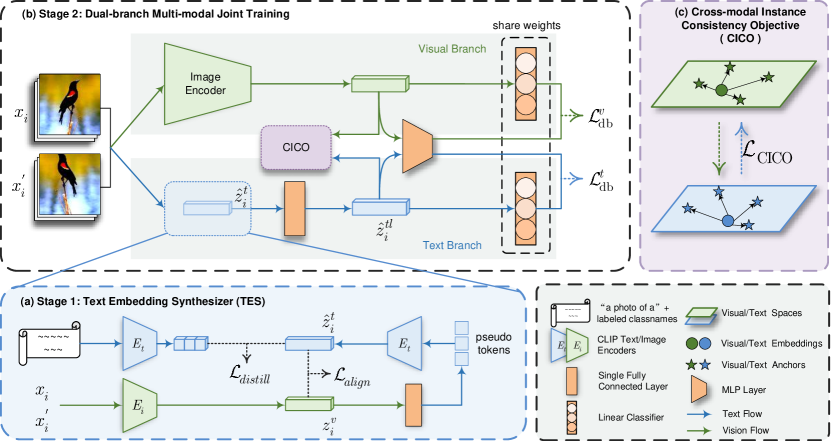
Figure 2: Overview of our GET framework. (a) In the first stage, we introduce a text embedding synthesizer that generates pseudo text embeddings for unlabelled data. TES learns a linear mapping that transforms image features into input tokens for the text encoder. The resulting pseudo text embeddings are then used for joint training in the second stage. (b) We proposed a dual-branch multi-modal joint training framework with a cross-modal instance consistency objective in the second stage. Two branches utilize the same parameterized training strategy [40] while focusing on text and visual information, respectively. (c) Our cross-modal instance consistency objective makes visual and text information exchange and benefit from each other.

The objective of TES contains an align loss on all samples and a distill loss on labeled samples. To align the generated pseudo text embeddings $\boldsymbol{\hat{z}}_{i}^{t}$ with their corresponding visual features $\boldsymbol{z}_{i}^{v}$, our align loss leverages the modality alignment property of CLIP’s encoders, pulling correct visual-text embedding pairs closer while pushing away the incorrect ones. The align loss consists of symmetric components $\mathcal{L}_{align}^{v}$ and $\mathcal{L}_{align}^{t}$, calculated as:

$$\mathcal{L}_{align}^{v}=-\frac{1}{|B|}\sum_{i\in B}\log\frac{\exp\left({\boldsymbol{z}_{i}^{v}}^{\top}{\boldsymbol{\hat{z}}_{i}^{t}}/\tau_{a}\right)}{\sum_{j\in B}\exp\left({\boldsymbol{z}_{i}^{v}}{\boldsymbol{\hat{z}}_{j}^{t}}/\tau_{a}\right)}\,,$$ (5)

$$\mathcal{L}_{align}^{t}=-\frac{1}{|B|}\sum_{i\in B}\log\frac{\exp\left({\boldsymbol{\hat{z}}_{i}^{t}}^{\top}{\boldsymbol{z}_{i}^{v}}/\tau_{a}\right)}{\sum_{j\in B}\exp\left({\boldsymbol{\hat{z}}_{i}^{t}},{\boldsymbol{z}_{j}^{v}}/\tau_{a}\right)}\,,$$ (6)

where $\boldsymbol{\hat{z}}_{i}^{t}$ and $\boldsymbol{z}_{i}^{v}$ are $\ell_{2}$-normalised, and $\tau_{a}$ is a temperature parameter. Thus, the align loss is $\mathcal{L}_{align}=\mathcal{L}_{align}^{v}+\mathcal{L}_{align}^{t}$ .

To ensure that our generated pseudo text features reside in the same embedding space as real text features and maintain consistency, we introduce a distill loss $\mathcal{L}_{distill}$:

$$\mathcal{L}_{distill}=-\frac{1}{|B_{l}|}\sum_{i\in B_{l}}\left(\log\frac{\exp\left({{\boldsymbol{\hat{z}}_{i}^{t}}^{\top}{T(n_{i})}}\right)}{\sum_{j=0}^{|\mathcal{Y}_{l}|}\mathbbm{1}_{[j\neq n_{i}]}\exp\left({\boldsymbol{\hat{z}}_{i}^{t}}^{\top}{T(j)}\right)}+\left(\boldsymbol{\hat{z}}_{i}^{t}-T(n_{i})\right)^{2}\right)\,,$$ (7)

where $T\in|\mathcal{Y}_{l}|\times dim$ are the real text embeddings of $|\mathcal{Y}_{l}|$ semantic labels, $n_{i}\in\mathcal{Y}_{l}$ indexes the corresponding class name of $\boldsymbol{x}_{i}$ among all known class names, $T(j)$ denotes the $j$-th real text embeddings of all known class names and $\mathbbm{1}_{[\cdot]}$ is the indicator function. Each vector in $T$ is produced by the text encoder using the prompt “a photo of a {cls}” where {cls} denotes the corresponding class name.

By aligning the pseudo text embeddings of labeled data and their corresponding real text embeddings, the pseudo text embeddings for unlabelled data can also implicitly align with the real embeddings. The overall objective of our text embedding synthesizer is calculated as:

$$\mathcal{L}_{TES}=\mathcal{L}_{align}+\mathcal{L}_{distill}\,.$$ (8)

The distill loss is used to guide pseudo text embeddings of the network’s output towards the real semantic corresponding space and adapt the model to the distribution of the dataset, while the align loss prevents overfitting to known classes and enforces the consistency between two modalities.

Moreover, we introduce a multi-view strategy for TES. Specifically, we calculate both the align loss $\mathcal{L}_{align}$ and distill loss $\mathcal{L}_{distill}$ for two different views $\boldsymbol{x}_{i}$ and ${\boldsymbol{x}_{i}}^{\prime}$ of the same image in a mini-batch. This further implicitly enhances the instance discriminative nature [42] of our TES training. This allows different views of the same image to generate identical pseudo text embeddings while aligning with their shared visual features. The generated pseudo text embeddings $\boldsymbol{\hat{z}}_{i}^{t}$ are then used for joint training in the second stage.

4.2 Dual-branch multi-modal joint training

Intuitively, the introduction of multi-modal information can have a positive impact on the GCD task. Categories with similar visual concepts may be distinguished on the basis of textual concepts. However, how to effectively utilize visual and text information in the GCD task and make the most of their respective roles remains challenging. In this paper, we propose a dual-branch architecture as illustrated in Fig. 2 (b), which focuses on semantic and visual information, respectively. We employ the same parametric training strategy (in Sec. 3.2) for each branch to promote that the model has aligned and complementary discriminative capabilities for visual and text features of the same class. Furthermore, we introduce a cross-modal instance consistency loss, which constrains the instance relationships of samples in both visual and text spaces, enabling the two branches to learn from each other. We use the indicator $v$ to represent the visual concept while $t$ for the text concept.

Visual-branch.

The objective of the visual branch contains a representation learning part and a parametric classification part. Given a visual embedding $\boldsymbol{z}_{i}^{v}$ of image $\boldsymbol{x}_{i}$ generated by the image encoder, an MLP layer $g(\cdot)$ is used to map $\boldsymbol{z}_{i}^{v}$ to a high-dimensional embedding $\boldsymbol{h}_{i}^{v}=g(\boldsymbol{z}_{i}^{v})$. Meanwhile, we employ a prototypical classifier $\eta(\cdot)$ to generate classification probability distribution $\boldsymbol{p}_{i}^{v}=\eta(\boldsymbol{z}_{i}^{v})$. Simply replace all the high-dimensional embedding $\boldsymbol{h}$ in Eqs. 1 and 2 with its corresponding visual branch version $\boldsymbol{h}^{v}$ can obtain the the supervised contrastive loss $\mathcal{L}_{scon}^{v}$ and the self-supervised contrastive loss $\mathcal{L}_{ucon}^{v}$. The overall representation learning loss is balanced with $\lambda$, written as:

$$\mathcal{L}_{\text{rep}}^{v}=(1-\lambda)\mathcal{L}_{ucon}^{v}+\lambda\mathcal{L}_{scon}^{v}\,.$$ (9)

For the parametric classification part, just replace $\boldsymbol{p}_{i}$ and ${\boldsymbol{p}_{i}}^{\prime}$ of Eq. 3 and Eq. 4 with $\boldsymbol{p}_{i}^{v}$ and ${\boldsymbol{p}_{i}^{v}}^{\prime}$ can obtain the cross-entropy loss $\mathcal{L}_{\text{cls-v}}^{s}$ and the self-distillation loss $\mathcal{L}_{\text{cls-v}}^{u}$. Thus, the classification loss is $\mathcal{L}_{\text{cls}}^{v}=(1-\lambda)\mathcal{L}_{\text{cls-v}}^{u}+\lambda\mathcal{L}_{\text{cls-v}}^{s}$.

The overall objective of visual branch is as:

$$\mathcal{L}_{\text{dual}}^{v}=\mathcal{L}_{\text{rep}}^{v}+\mathcal{L}_{\text{cls}}^{v}\,.$$ (10)

Text-branch.

Our text branch simply adopts the same training strategy as the visual branch. That is, in particular, given a text embedding $\boldsymbol{\hat{z}}_{i}^{t}$ generated by TES, we first input it into a fully connected layer to gain a learnable text embedding $\boldsymbol{\hat{z}}_{i}^{tl}$ while change its dimension. Simply replace $\boldsymbol{h}_{i}^{v}$ in the representation learning objective $\mathcal{L}_{\text{rep}}^{v}$ with $\boldsymbol{h}_{i}^{t}=g(\boldsymbol{\hat{z}}_{i}^{tl})$ and replace ${\boldsymbol{p}_{i}^{v}}$ in classification parts $\mathcal{L}_{\text{cls}}^{v}$ with $\boldsymbol{p}_{i}^{t}=\eta(\boldsymbol{\hat{z}}_{i}^{tl})$ can yield the corresponding text objectives $\mathcal{L}_{\text{rep}}^{t}$ and $\mathcal{L}_{\text{cls}}^{t}$. In other words, changing the visual conception indicator $v$ into text conception indicator $t$ can get the corresponding objectives for the text branch. Thus, the overall objective of our text branch can be formally written as:

$$\mathcal{L}_{\text{dual}}^{t}=\mathcal{L}_{\text{rep}}^{t}+\mathcal{L}_{\text{cls}}^{t}\,.$$ (11)

To mitigate the bias between old and new classes, we extended the mean-entropy regularization [1] to a multi-modal mean entropy regularization $H_{mm}={H}(\overline{p}_{mm},\overline{p}_{mm})$, here $\overline{p}_{mm}$ can calculate by $\overline{p}_{mm}=\frac{1}{2|B|}\sum_{i\in B}\left(\sigma({\boldsymbol{p}_{i}^{v}},\tau_{s})+\sigma(\boldsymbol{p}_{i}^{t},\tau_{s})\right)$. In this way, the prediction probabilities in different modalities for each prototype are constrained to be the same, preventing trivial solution.

Cross-modal instance consistency objective.

In order to enable the two branches to learn from each other while encouraging agreement between two different modes, we propose a cross-modal instance consistency objective (CICO), shown in Fig. 2 (c). Our CICO has the same form of mutual knowledge distillation as  [44], but we distill the instance consistency between the two branches. For each mini-batch $B$, we choose its labeled subset $B_{l}$ containing $K$ categories as anchor samples, calculate the visual and text prototypes for $K$ categories as visual anchors $\mathcal{P}_{v}$ and text anchors $\mathcal{P}_{t}$, respectively. We define the instance relationships in visual and text branch as:

$$s_{i}^{v}=\sigma(sim(\boldsymbol{z}_{i}^{v},\mathcal{P}_{v})\,,$$ (12)

$$s_{i}^{t}=\sigma(sim(\boldsymbol{\hat{z}}_{i}^{tl},\mathcal{P}_{t}))\,.$$ (13)

Thus our CICO can formally written as:

$$\mathcal{L}_{\text{CICO}}=\frac{1}{2|B|}\sum_{i\in B}\left(D_{KL}(s_{i}^{t}||s_{i}^{v})+D_{KL}(s_{i}^{v}||s_{i}^{t})\right)\,,$$ (14)

where $D_{KL}$ is the Kullback-Leibler divergence. Mutual knowledge distillation on instance relationships for two modalities makes visual and text flows exchange and benefit from each other, which is demonstrated to be effective in Sec. 5.3.

The overall optimization objective of our method is:

$$\mathcal{L}_{\text{Dual}}=\mathcal{L}_{\text{dual}}^{v}+\mathcal{L}_{\text{dual}}^{t}-\lambda_{h}H_{mm}+\lambda_{c}\mathcal{L}_{\text{CICO}}\,.$$ (15)

5 Experiments

5.1 Experimental setup

Datasets. We evaluate our method on multiple benchmarks, including three image classification generic datasets (i.e., CIFAR 10/100 [20] and ImageNet-100 [8]), three fine-grained datasets from Semantic Shift Benchmark [37] (i.e., CUB [39], Stanford Cars [19] and FGVC-Aircraft [27]), and three challenging datasets (i.e., Herbarium 19 [35], ImageNet-R [15] and ImageNet-1K [8]). Notice that we are the first to introduce ImageNet-R into the GCD task, which contains various renditions of 200 ImageNet classes, thus challenging the GCD’s assumption that the data comes from the same domain. The details of the datasets we evaluate on are reported in Supplementary Materials (SM).

Evaluation metrics.

Following standard evaluation protocol (V2) in [36], we evaluate the performance with clustering accuracy (ACC), calculated as:

$$\mathcal{ACC}=\max_{perm\in\mathcal{P}}\frac{1}{|\mathcal{D}_{u}|}\sum_{i=1}^{|\mathcal{D}_{u}|}\mathbbm{1}{[y_{i}=perm(\hat{y}_{i})]}\,,$$ (16)

where $y_{i}$ and $\hat{y}_{i}$ represent the ground-truth and predicted label, respectively. $\mathcal{P}$ is the set of all permutations while the optimal can be computed with the Hungarian algorithm [22].

Implementation details.

We use a ViT-B/16 [9] pre-trained with CLIP [32] as the backbone of the image and text encoder. In the first stage, we train a fully connected layer to transfer image embeddings into pseudo tokens. In the second stage, we use a single linear layer to turn pseudo text embeddings generated by TES into learnable embeddings while changing their dimensions to match those of the visual features. Our dual-branch training implementation details simply follow previous [40, 36] and are presented in SM. The last-epoch visual branch is used for evaluation and we provide the pseudocode in SM to clearly describe the details of the training and testing.

5.2 Comparison with state of the arts

In this section, we compare the proposed GET with the several state-of-the-art methods, including: $k$-means [26], RS+ [13], UNO+ [11], ORCA [2], PromptCAL [43], DCCL [31], GPC [46], GCD [36] and SimGCD [40]. GCD [36] and SimGCD [40] provide paradigms for non-parametric and parametric classification, thus we replace their backbone with CLIP for a fair comparison, denoted as GCD-CLIP and SimGCD-CLIP.

Evaluation on fine-grained datasets.

As shown in Tab. 1, our method achieves remarkable success on all three fine-grained datasets. Specifically, we surpass SimGCD-CLIP by 5.3%, 8.5%, and 4.6% on ‘All’ classes of CUB, Stanford Cars, and Aircraft, respectively. In fine-grained datasets, the visual conceptions of distinct classes exhibit high similarity, making it challenging for classification based solely on visual information. However, their text information is notably different. Consequently, our GET  significantly enhances classification accuracy through the reciprocal augmentation of text and visual information flow. More qualitative results are reported in SM.

Table 1: Results on fine-grained and generic datasets.

	CUB			Stanford Cars			FGVC-Aircraft			CIFAR10			CIFAR100			ImageNet-100
Methods	All	Old	New	All	Old	New	All	Old	New	All	Old	New	All	Old	New	All	Old	New
$k$-means [26]	34.3	38.9	32.1	12.8	10.6	13.8	16.0	14.4	16.8	83.6	85.7	82.5	52.0	52.2	50.8	72.7	75.5	71.3
RS+ [13]	33.3	51.6	24.2	28.3	61.8	12.1	26.9	36.4	22.2	46.8	19.2	60.5	58.2	77.6	19.3	37.1	61.6	24.8
UNO+ [11]	35.1	49.0	28.1	35.5	70.5	18.6	40.3	56.4	32.2	68.6	98.3	53.8	69.5	80.6	47.2	70.3	95.0	57.9
ORCA [2]	35.3	45.6	30.2	23.5	50.1	10.7	22.0	31.8	17.1	81.8	86.2	79.6	69.0	77.4	52.0	73.5	92.6	63.9
GCD [36]	51.3	56.6	48.7	39.0	57.6	29.9	45.0	41.1	46.9	91.5	97.9	88.2	73.0	76.2	66.5	74.1	89.8	66.3
GPC [46]	55.4	58.2	53.1	42.8	59.2	32.8	46.3	42.5	47.9	92.2	98.2	89.1	77.9	85.0	63.0	76.9	94.3	71.0
DCCL [31]	63.5	60.8	64.9	43.1	55.7	36.2	-	-	-	96.3	96.5	96.9	75.3	76.8	70.2	80.5	90.5	76.2
PromptCAL [43]	62.9	64.4	62.1	50.2	70.1	40.6	52.2	52.2	52.3	97.9	96.6	98.5	81.2	84.2	75.3	83.1	92.7	78.3
SimGCD [40]	60.3	65.6	57.7	53.8	71.9	45.0	54.2	59.1	51.8	97.1	95.1	98.1	80.1	81.2	77.8	83.0	93.1	77.9
GCD-CLIP	57.6	65.2	53.8	65.1	75.9	59.8	45.3	44.4	45.8	94.0	97.3	92.3	74.8	79.8	64.6	75.8	87.3	70.0
SimGCD-CLIP	71.7	76.5	69.4	70.0	83.4	63.5	54.3	58.4	52.2	97.0	94.2	98.4	81.1	85.0	73.3	90.8	95.5	88.5
GET (Ours)	77.0	78.1	76.4	78.5	86.8	74.5	58.9	59.6	58.5	97.2	94.6	98.5	82.1	85.5	75.5	91.7	95.7	89.7

Evaluation on generic datasets.

In Tab. 1, we also present the performances for three generic datasets. Due to the low resolution of the CIFAR dataset and model biases(CLIP itself performs poorly on CIFAR100, with a zero-shot performance of 68.7), the results for novel classes are inferior compared to the DINO backbone. However, despite the inherent limitations in the discriminative capability of CLIP itself, our method still achieves an improvement of 0.4% on ‘Old’ classes of CIFAR10 and 2.2% on ‘New’ classes of CIFAR100, compared to SimGCD-CLIP. For ImageNet-100, SimGCD-CLIP has achieved an exceptionally saturated result of 90.8% on ‘All’ classes, further advancements pose considerable challenges. However, leveraging the additional modality information, GET elevates the performance ceiling to an impressive 91.7%.

Table 2: Results on more challenging datasets.

	Herbarium 19			ImageNet-1K			ImageNet-R
Methods	All	Old	New	All	Old	New	All	Old	New
$k$-means [26]	13.0	12.2	13.4	-	-	-	-	-	-
RS+ [13]	27.9	55.8	12.8	-	-	-	-	-	-
UNO+ [11]	28.3	53.7	14.7	-	-	-	-	-	-
ORCA [2]	20.9	30.9	15.5	-	-	-	-	-	-
GCD [36]	35.4	51.0	27.0	52.5	72.5	42.2	32.5	58.0	18.9
SimGCD [40]	44.0	58.0	36.4	57.1	77.3	46.9	29.5	48.6	19.4
GCD-CLIP	37.3	51.9	29.5	55.0	65.0	50.0	44.3	79.0	25.8
SimGCD-CLIP	48.9	64.7	40.3	61.0	73.1	54.9	54.9	72.8	45.3
GET (Ours)	49.7	64.5	41.7	62.4	74.0	56.6	58.1	78.8	47.0

Evaluation on challenging datasets.

We further evaluate on three challenging datasets. As shown in Tab. 2, GET outperforms all other state-of-the-art methods for both ‘All’ and ‘New’ classes on Herb19 and ImageNet-1K datasets. In particular, our method achieves a notable improvement of 1.4% and 1.7% on ‘New’ classes of Herb19 and ImageNet-1K, respectively. Furthermore, the suboptimal performance of GCD and SimGCD with the DINO backbone on the ImageNet-R dataset highlights the difficulty of DINO in discovering new categories with multiple domains. Despite multiple domains for images of the same category, their textual information remains consistent. Our method effectively integrates text information, resulting in a substantial improvement of 3.2% and 6.0% over the state-of-the-art for ‘All’ classes and ‘Old’ classes, respectively. It is worth noting that, owing to the text consistency within the same category, our text branch achieves remarkable 62.6% and 63.5% accuracy for ‘All’ classes of Imagenet-R and ImageNet-1K, respectively. The detailed results of the text branch can be seen in SM.

5.3 Ablation study and analysis

Effectiveness of different components.

To evaluate the effectiveness of different components, we conduct an ablation study on Stanford Cars and CIFAR100 in Tab. 3. Comparing (2) with (1), the dual-branch training strategy can effectively leverage the text features generated by TES, resulting in a 6.2% improvement on Scars’ ‘All’ classes and a 0.3% improvement on CIFAR100’s ‘Old’ classes. Furthermore, comparing (3) with (1), CICO enables the two branches to exchange information and mutually benefit from each other, resulting in remarkable improvements of 11% on Scars’ ‘New’ and 2.2% on CIFAR100’s ‘New’.

Table 3: Ablation study of different components.

	TES	Dual-branch	CICO	Stanford Cars			CIFAR100
				All	Old	New	All	Old	New
(1)	✗	✗	✗	70.0	83.4	63.5	81.1	85.0	73.3
(2)	✓	✓	✗	76.2	85.3	71.7	81.0	85.3	72.3
(3)	✓	✓	✓	78.5	86.8	74.5	82.1	85.5	75.5

Effectiveness of text embedding synthesizer.

In order to prove that our text embedding synthesizer can generate reliable and discriminative representations, we visualize the text embeddings of CIFAR10 with t-SNE. As shown in Fig. 3, the initial text embeddings within the same class exhibit clear clustering, and the learnable embeddings further produce compacter clusters. Moreover, we introduce TES into the non-parametric GCD by straightforwardly concatenating text and image features before semi-supervised k-means classification. As in Tab. 4, with the help of text information, GCD gains about 5% average improvement on ‘All’ classes over 3 datasets, demonstrating the importance of multi-modal information in GCD task and our TES can be widely used in multiple GCD methods. We provide more results and analysis for TES in SM.

Table 4: Effectiveness of TES in non-parametric GCD.

	FGVC-Aircraft			ImageNet-100			ImageNet-R
Methods	All	Old	New	All	Old	New	All	Old	New
GCD-CLIP	45.3	44.4	45.8	75.8	87.3	70.0	44.3	79.0	25.8
+TES	49.6	49.3	49.8	80.0	95.1	72.4	49.4	79.4	33.5

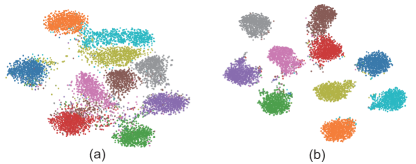
Figure 3: t-SNE visualization of text features for all classes on CIFAR10 test set. (a) shows the distribution of text features generated by TES, while (b) shows the learnable text features.

Comparison with different fusion methods.

In Tab. 5, we compare our dual-branch training strategy with other methods that fuse visual and text features, including concatenation and mean. Although they may show improvements in ‘Old’ or ‘New’ classes due to the multi-modal information, we demonstrate that joint learning of the two branches is more effective as it encourages the model to have complementary and aligned discriminative capabilities for visual and text features of a same class, leading to more discriminative multi-modal prototypes and more cohesive multi-modal clusters.

Table 5: Comparison with different fusion methods.

	Dual-branch	Concat	Mean	Stanford Cars			CIFAR100
				All	Old	New	All	Old	New
(1)	✗	✓	✗	68.9	79.1	64.0	79.9	85.5	68.7
(2)	✗	✗	✓	72.0	85.0	65.6	81.1	84.3	74.8
(3)	✓	✗	✗	78.5	86.8	74.5	82.1	85.5	75.5

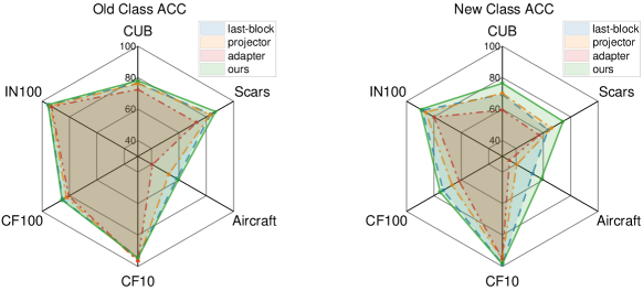
Figure 4: Different ViT finetune strategies.

Different ViT fine-tuning strategies.

GCD [36] and SimGCD [40] propose to build the classifier on post-backbone features instead of post-projector. Because the ViT backbone of CLIP contains a lot of knowledge learned from substantial image-text pairs, and the projector plays a role in modal alignment, it’s essential to compare the effects of different ViT finetune strategies. As shown in Fig. 4, we conduct multiple evaluations with last-block fine-tuning, projector fine-tuning, and adapter [12] fine-tuning strategies. Though simply fine-tuning the projector can gain a higher accuracy across CUB and Aircraft datasets, it falls behind the last-block fine-tuning method for generic datasets. Overall, our GET perfoms the best among all methods. For a fair comparison, we select the last-backbone fine-tuning strategy for baseline methods and our dual-branch multi-modal learning across all datasets except projector fine-tuning for ImageNet-1K. The detailed results of different fine-tuning strategies are posted in SM.

5.4 Different pre-trained models

In this section, we conduct extensive experiments to investigate how different types of backbones influence the GCD task. As shown in Fig. 5, we evaluate the results of GCD and SimGCD across different types of pretraining models, including DINO [4], which is based on teacher-student learning; MoCo v3 [6], based on contrastive learning; iBOT [47], based on masked image modeling; and CLIP [32], which is based on vision-language contrastive learning. Different types of backbones exhibit varying biases across different datasets, classes, and even paradigms. A key observation is that though promising results have been achieved, different backbones, even powerful CLIP, still perform inferiorly on distinguishing certain visually similar classes, such as the classes in all fine-grained datasets. We argue that this is due to current methods only utilizing a single visual modality of information, another modality may potentially compensate for the lack of discriminative ability. Due to CLIP’s multi-modal training strategy and its strong generalization ability, we decide to introduce it into the GCD task. This not only unleashes the latent potential performance of existing methods but also serves as a bridge for us to leverage multi-modal information. Detailed analysis and additional visualization results are available in SM.

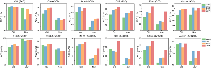
Figure 5: The results of GCD and SimGCD with different backbones across six datasets.

6 Conclusions

In this paper, we propose to leverage multi-modal information to solve the GCD task. In particular, we introduce a text embedding synthesizer to generate pseudo text embeddings for unlabelled data. Our TES module makes it possible to use CLIP’s text encoder, thus unlocking the multi-modal potential of CLIP for the GCD task. Meanwhile, we use a dual-branch training strategy with a cross-modal instance consistency objective, which facilitates collaborative action and mutual learning between the different modalities, thus generating more discriminative classification prototypes. The superior performance on multiple benchmarks demonstrates the effectiveness of our method.

7 Acknowledgments

This work is funded by NSFC (NO. 62225604, 62206135, 62202331), and the Fundamental Research Funds for the Central Universities (Nankai Universitiy, 070-63233085). Computation is supported by the Supercomputing Center of Nankai University.

Supplementary Materials

The Supplementary Materials includes the following sections. First, we introduce our dataset details and training details in Sec. 0.A. Then, we provide more experiment results and analysis in Sec. 0.B. We further discuss the utilization of CLIP in GCD and the intuition behind our TES in Sec. 0.C, and we prove that our TES can deal with a scenario where CLIP lacks information on a specific category class. We provide the pseudo-code in Sec. 0.D. Sec. 0.E shows the visualization of different pre-trained models while Sec. 0.F shows the qualitative results of our method. Finally, we provide the broader impact and limitations in Sec. 0.G.

Appendix 0.A Implementation Details

0.A.1 Dataset details

As shown in Tab. 6, we evaluate our method on multiple benchmarks. We introduced ImageNet-R [15] to the GCD task to demonstrate that GCD based on multi-modal features can generalize across different domains. For ImageNet-R, we subsample the first 100 classes as old classes, leaving the rest as new classes; the labeled dataset $\mathcal{D}_{l}$ consists of half of the old class samples, while the other half and all the new class samples are used to construct unlabelled dataset $\mathcal{D}_{u}$. As for other benchmarks, we follow the previous [36, 40] to sample $\mathcal{D}_{l}$ and $\mathcal{D}_{u}$. ImageNet-R contains various renditions (including art, cartoons, deviantart, graffiti, embroidery, graphics, origami, paintings, patterns, plastic objects, plush objects, sculptures, sketches, tattoos, toys, and video game.) of 200 ImageNet classes resulting in 30,000 images. The statistics for ImageNet-R are shown in Fig. 6. In our experiment, we only sample classes from the set of categories in ImageNet-R to construct labeled dataset $\mathcal{D}_{l}$ and unlabelled dataset $\mathcal{D}_{u}$, without sampling domains. That means, whether old classes or new classes, data from the same category might have multiple domains.

Table 6: The details of the datasets we evaluate on.

	Labelled		Unlabelled
Dataset	Images	Classes	Images	Classes
CIFAR10 [20]	12.5K	5	37.5K	10
CIFAR100 [20]	20.0K	80	30.0K	100
ImageNet-100 [8]	31.9K	50	95.3K	100
CUB [39]	1.5K	100	4.5K	200
Stanford Cars [19]	2.0K	98	6.1K	196
FGVC-Aircraft [27]	1.7K	50	5.0K	100
Herbarium 19 [35]	8.9K	341	25.4K	683
ImageNet-R [15]	7.7K	100	22.3K	200
ImageNet-1K [8]	321K	500	960K	1000

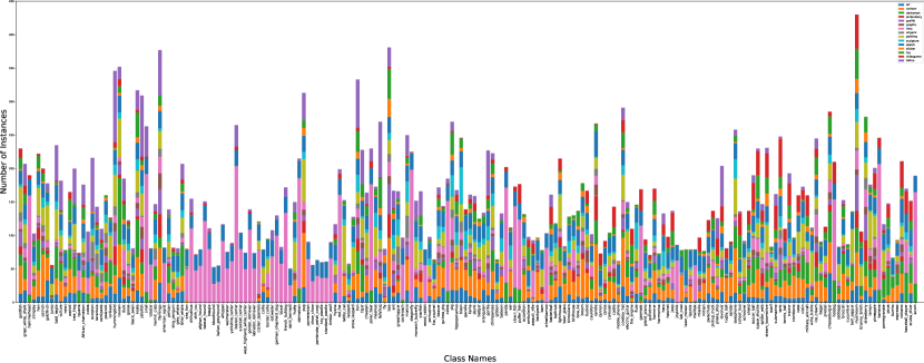
Figure 6: The statistics for ImageNet-R.

0.A.2 Training details

Following [36] and [40], we only fine-tune the last transformer block of the image encoder for all datasets resulting in features with a dimension of 768. The exception is ImageNet-1K, we only fine-tune the last projection layer, resulting in features with a dimension of 512. When fine-tuning the last block of the CLIP visual encoder for ImageNet-1K, there is a risk of gradient explosion. Meanwhile, fine-tuning the last projection layer instead can lead to better results than fine-tuning the last block using a lower learning rate. Additionally, fine-tuning the last projection layer requires fewer computational resources. Therefore, we chose to fine-tune only the last projection layer for ImageNet-1K. The batch size is fixed to 128 for training and 256 for testing. Training is done with an SGD optimizer and an initial learning rate of 0.1 decayed by a cosine annealing rule. We train for 200 epochs on each dataset in both two stages. In the first stage, we set the number of pseudo text tokens to 7. The balance coefficient $\lambda$ is set to 0.35 as [36], while $\lambda_{h}$ and $\lambda_{c}$ are set to 2 and 1, respectively. The temperature value $\tau_{a}$ is set to 0.01 while other temperature values $\tau_{c}$, $\tau_{s}$ and $\tau_{t}$ are as same as [40]. All experiments are conducted with 4 NVIDIA GeForce RTX 3090 GPUs.

Appendix 0.B Additional Experiment Results and Analysis

0.B.1 Error bars for main results

The experimental results presented in the paper are the averages of three independent repeated runs. We provide the performance standard deviation of our main results on all evaluation datasets with three runs in Tab. 7.

Table 7: The standard deviation of our method.

Dataset	All	Old	New
CIFAR10	97.2$\pm$0.1	94.6$\pm$0.1	98.5$\pm$0.1
CIFAR100	82.1$\pm$0.4	85.5$\pm$0.5	75.5$\pm$0.5
ImageNet-100	91.7$\pm$0.3	95.7$\pm$0.0	89.7$\pm$0.4
CUB	77.0$\pm$0.5	78.1$\pm$1.6	76.4$\pm$1.2
Stanford Cars	78.5$\pm$1.3	86.8$\pm$1.5	74.5$\pm$2.2
FGVC-Aircraft	58.9$\pm$1.2	59.6$\pm$0.6	58.5$\pm$1.8
Herbarium 19	49.7$\pm$0.4	64.5$\pm$0.8	41.7$\pm$0.8
ImageNet-1K	62.4$\pm$0.0	74.0$\pm$0.2	56.6$\pm$0.1
ImageNet-R	58.1$\pm$2.4	78.8$\pm$0.5	47.0$\pm$3.9

0.B.2 Additional baseline results

As shown in Tab. 8. We provide results of PromptCAL-CLIP on three fine-grained datasets and three image classification generic datasets. For three fine-grained datasets, our method outperforms PromptCAL-CLIP on all datasets and classes. In particular, we surpass PromptCAL-CLIP by 11.5%, 4.5%, and 4.4% on ‘All’ classes of CUB, Stanford Cars, and Aircraft, respectively. As for the generic datasets, our method surpasses PromptCAL-CLIP on all datasets and achieves the best results on CIFAR-100 and ImageNet-100 datasets.

Table 8: Results of PromptCAL-CLIP.

	CUB			Stanford Cars			FGVC-Aircraft			CIFAR10			CIFAR100			ImageNet-100
Methods	All	Old	New	All	Old	New	All	Old	New	All	Old	New	All	Old	New	All	Old	New
PromptCAL [43]	62.9	64.4	62.1	50.2	70.1	40.6	52.2	52.2	52.3	97.9	96.6	98.5	81.2	84.2	75.3	83.1	92.7	78.3
PromptCAL-CLIP	65.5	68.7	63.9	74.0	80.8	70.8	54.5	61.8	51.0	88.7	96.5	84.8	80.5	82.4	76.8	87.4	93.6	84.3
GET (Ours)	77.0	78.1	76.4	78.5	86.8	74.5	58.9	59.6	58.5	97.2	94.6	98.5	82.1	85.5	75.5	91.7	95.7	89.7

0.B.3 Results of two branches

We report the results of visual and text branches for ‘All’ classes across six datasets in Tab. 9. For 2 generic datasets (CIFAR10 and ImageNet-100), though the text branch does not achieve state-of-the-art performance, it still exhibits great performance. For 2 fine-grained datasets (CUB and Stanford Cars), both visual and text branches outperform previous methods by a large margin, while the visual branch performs better. For 2 challenging datasets (ImageNet-1K and ImageNet-R), both visual and text branches achieve remarkable results. Due to the challenging datasets comprising a significant number of unknown classes (ImageNet-1k dataset) or diverse visual concepts within the same class (ImageNet-R dataset), the consistency in text information for the same class contributes to the potentially higher discriminative power of the text branch, leading to a better performance for text branch.

Table 9: The results of two branches.

Dataset	Visual Branch	Text Branch
CIFAR10	97.2$\pm$0.1	95.1$\pm$0.0
ImageNet-100	91.7$\pm$0.3	90.1$\pm$0.1
CUB	77.0$\pm$0.5	73.6$\pm$0.8
Stanford Cars	78.5$\pm$1.3	73.1$\pm$0.6
ImageNet-1K	62.4$\pm$0.0	63.5$\pm$0.1
ImageNet-R	58.1$\pm$2.4	62.6$\pm$0.9

We also provide the performance evolution of two branches throughout the model learning process on the CUB dataset (see in  Fig. 7), the mutual promotion and fusion of the two branches resulted in excellent outcomes. In our experiments, we consistently and simply select the results from the visual branch.

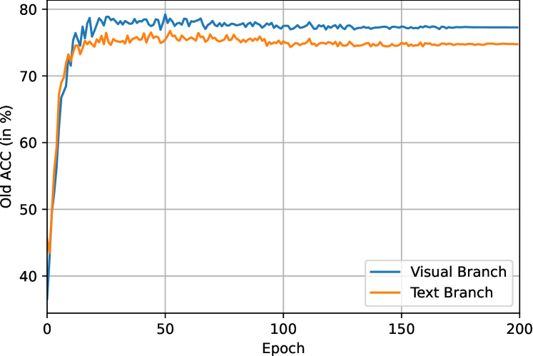
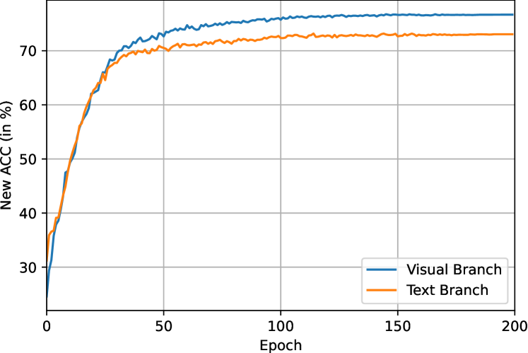
Figure 7: Performance evolution of two branches throughout the model learning process on the CUB dataset

0.B.4 Estimation of class number in unlabelled data.

Vaze et al. [36] provides an off-the-shelf method to estimate the class number in unlabelled data. We introduce text embeddings generated by our TES into the off-the-shelf method by simply concatenating text and image features before class number Estimation. As shown in Tab. 10, multi-modal features can estimate a more accurate class number than single visual features, demonstrating our multi-modal method is effective in category number estimation.

Table 10: Estimation of class number in unlabelled data. We use an off-the-shelf method provided by Vaze et al. [36] to estimate the class number in unlabelled data. The table shows the estimated number and the error.

Method	CIFAR-10	CIFAR-100	ImageNet-100	CUB-200	SCars
Ground truth	10	100	100	200	196
GCD-CLIP	5 (50%)	94 (6%)	116 (16%)	212 (12%)	234 (19%)
$+$TES	8 (20%)	97 (3%)	109 (9%)	212 (12%)	220 (12%)

0.B.5 Results of different ViT fine-tuning strategies

We reported the detailed results of different fine-tuning strategies based on SimGCD-CLIP in Tab. 11. Only fine-tuning an additional adapter proved insufficient to fully leverage the performance of the pre-trained model, hence yielding the poorest results. While fine-tuning the projection layer can achieve good results with relatively low computational resources on the CUB and Stanford Cars datasets, its performance on other datasets is significantly inferior to fine-tuning the last block of the model, thus we choose the last-block fine-tuning strategy for baseline methods on most datasets.

Table 11: Results of different ViT fine-tuning strategies.

	CUB			Stanford Cars			FGVC-Aircraft			CIFAR10			CIFAR100			ImageNet-100
Methods	All	Old	New	All	Old	New	All	Old	New	All	Old	New	All	Old	New	All	Old	New
last-block	71.7	76.5	69.4	70.0	83.4	63.5	54.3	58.4	52.2	97.0	94.2	98.4	81.1	85.0	73.3	90.8	95.5	88.5
projector	72.2	76.3	70.1	71.5	83.0	65.9	44.6	52.6	40.5	95.6	96.3	95.2	77.1	82.3	66.7	88.7	93.9	86.0
adapter	63.9	72.5	59.5	62.1	72.9	56.9	37.1	40.7	35.3	95.6	96.4	95.2	74.2	80.6	61.6	84.3	93.2	79.8
GET (Ours)	77.0	78.1	76.4	78.5	86.8	74.5	58.9	59.6	58.5	97.2	94.6	98.5	82.1	85.5	75.5	91.7	95.7	89.7

0.B.6 Computation complexity analysis.

Tab. 12 shows the computation complexity. Our TES uses a frozen visual encoder and stage 2 finetunes the last block in another visual encoder, thus the 2 stages share the same visual encoder for the first 11 blocks but a different last block, resulting in a low computational complexity increase.

Table 12: Computation complexity analysis

	Inference Time	Learnable Params	FLOPs
Methods	(s/per img)	(M)	(G)
SimGCD-CLIP	$\text{5.2}\times\text{10}^{-\text{3}}$	13.4	35.2
GET(ours)	$\text{5.2}\times\text{10}^{-\text{3}}$	15.6	38.6

0.B.7 Analysis of loss components in TES

The objective of our TES module contains an align loss on all samples and a distill loss on labeled samples. The align loss $\mathcal{L}_{align}$ leverages the modality alignment property of CLIP’s encoders, aligning the generated pseudo-text embeddings with their corresponding visual feature. The distill loss $\mathcal{L}_{distill}$ is used to guide pseudo text embeddings of the network’s output towards the real semantic corresponding space and adapt the model to the distribution of the dataset. As shown in Tab. 13, utilizing either distillation loss or alignment loss independently in TES followed by a dual-branch training does not yield performance as strong as the combination of both losses.

Table 13: Ablation study of loss components in TES.

	$\mathcal{L}_{align}$	$\mathcal{L}_{distill}$	CUB
			All	Old	New
(1)	✗	✓	74.7	76.9	73.5
(2)	✓	✗	75.3	77.5	74.2
(3)	✓	✓	77.0	78.1	76.4

0.B.8 Experiments on pseudo-text token quantities in TES

We set the number of pseudo-text tokens in TES to 7 across all datasets. Experiment results on token quantities for the CUB dataset are presented in Fig. 8.

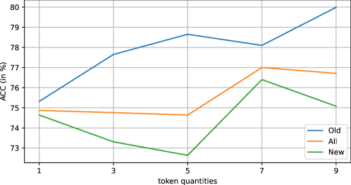
Figure 8: Experiment results on token quantities for the CUB dataset.

0.B.9 Experiments on the Clevr-4 dataset

Recently, [38] presented a synthetic dataset Clevr-4 to examine whether the GCD method can extrapolate the taxonomy specified by the labeled set. Most attributes of Clevr-4, such as shape, color, and count, are easily clustered (achieving close to 99% accuracy with CLIP). However, texture attributes pose a certain level of challenge. Therefore, we evaluate our method on the texture attributes of Clevr-4. As shown in Tab. 14, our method achieves higher accuracy and lower standard deviation compared to SimGCD-CLIP, proving that the GCD method can cluster data at specified levels based on the constraint of labeled text information, which is worthy of attention and exploration.

Table 14: The results on Clevr-4 (Texture) in 5 runs.

Methods	All	Old	New
SimGCD-CLIP	83.1$\pm$7.4	99.2$\pm$0.3	75.1$\pm$10.9
GET(ours)	90.0$\pm$1.9	99.2$\pm$0.2	85.5$\pm$2.8

Appendix 0.C Discussion about CLIP in GCD and our TES

A key purpose of GCD is to discover novel classes, which highly rely on the initial representation discrimination provided by the backbone model. CLIP, as a large model, is trained on a huge amount of image-text pairs covering broad a set of visual concepts. Due to the strong generalization ability of CLIP, it can encode more discriminative features, making it a natural idea to introduce CLIP into the GCD task. One concern is that CLIP may have seen unknown classes/claseenames in GCD. We contend that, as a general-purpose large model, careful consideration of how to effectively unleash its potential in specific tasks is a more worthy pursuit. While CLIP may have seen unknown classes (names), the issue of being unable to use the text encoder impedes its formidable performance. Our TES provides a way to leverage the CLIP text encoder without text input, thus unlocking the multi-modal potential of CLIP.

Furthermore, we try to prove our TES can deal with a scenario where CLIP lacks information on a specific category class. Since CLIP saw most of the visual concepts and corresponding texts before 2022, we constructed a small dataset of new energy vehicles (NEV) that appeared in 2023. The NEV dataset contains 12 categories, each with 50 images from the Internet, and the classnames (Tab. 15) of the dataset consist of the brand and model of the car. We split them in the same way as standard benchmarks.

Table 15: The classnames for the NEV dataset.

Old classes	New classes
BMW_xDrive_M60	Geely_Jiyue_01
BYD_Seagull	Geely_Zeeker_X
BYD_Song_L	Mercedes-Benz_EQE_SUV
BYD_Yangwang_U8	SAIC-Motor_MG_Cyberster
GAC-Motor_Trumpchi_ES9	SAIC-Motor_Rising_F7
Geely_Galaxy_E8	XPeng_X9

As shown in Tab. 16, due to the lack of information on the NEV dataset in CLIP, achieving only 10% zero-shot accuracy across all classes and CLIP can only recognize 5 out of the 12 categories. Due to the dataset’s fine-grained nature and few samples, SimGCD with the DINO backbone performs poorly on ‘New’ categories. Although fine-tuning with CLIP’s visual encoder as the backbone can yield great results, our GET with multi-modal features demonstrates a 9.7% improvement on ‘New’ categories. This proves the effectiveness of our TES in scenarios where CLIP lacks information or the CLIP text encoder has not encountered corresponding class names.

Table 16: The results on the NEV dataset.

CLIP zero-shot performance       10.7
GCD performance
Methods	All	Old	New
SimGCD	54.7	88.0	38.0
SimGCD-CLIP	79.1	96.7	70.3
GET(ours)	85.3	96.0	80.0

The intuition behind our TES can be explained from two perspectives, as illustrated in Fig. 9. The first perspective is that our trained TES can be considered as a special fine-tuned text encoder. This text encoder takes visual images as input and produces corresponding textual features as output. Our align loss ensures modal alignment, while the distill loss facilitates the model’s adaptation to the dataset’s distribution. The second perspective is that TES can be regarded as a caption model [28]. For each input image, TES assigns a corresponding caption, expressing each caption in the form of text features. The text embeddings or captions corresponding to images can serve as valuable supplementary information, assisting the GCD task in a multimodal manner.

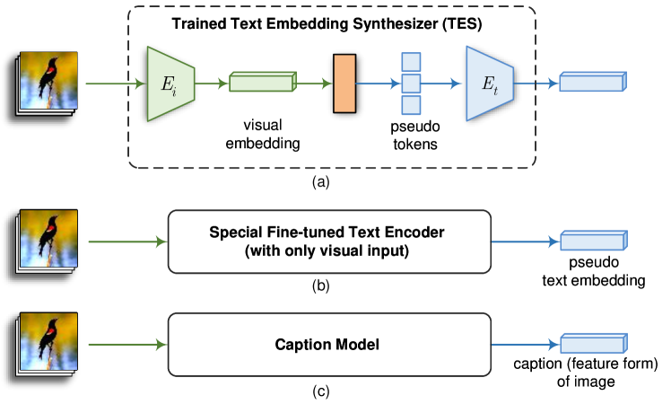
Figure 9: The intuition behind our TES. (a) Well-trained TES module; (b) TES can be considered as a special fine-tuned text encoder; (c) TES can be regarded as a caption model.

Appendix 0.D Pseudo-code

We provide a pseudo-code of our method in Algorithm 1. Since information from different modalities is exchanged and learned through CICO and injected into the trainable visual backbone, we utilize the last-epoch visual branch for inference. Specifically, passing unlabeled data through the trained visual encoder $f_{v}(\cdot|\theta_{\text{v}})$ and classifier $\eta(\cdot|\theta_{\text{c}})$ followed by the Hungarian algorithm can obtain the clustering results.

1

Input: Training dataset $\mathcal{D}$ contains labeled dataset $\mathcal{D}_{l}$ and unlabelled dataset $\mathcal{D}_{u}$, a FC layer $l(\cdot|\theta_{\text{t}})$ and a MLP layer $g(\cdot|\theta_{\text{m}})$, CLIP’s image encoder $f_{v}(\cdot|\theta_{\text{v}})$ and text encoder $f_{t}(\cdot)$, a classifier $\eta(\cdot|\theta_{\text{c}})$ and a linear projection $p(\cdot|\theta_{\text{p}})$.

2

Output: Trained backbone $f_{v}(\cdot|\theta_{\text{v}})$ and classifier $\eta(\cdot|\theta_{\text{c}})$.

3

/* Stage 1: TES Training */

4 for each epoch $e$=1…$E_{1}$  do

5       for  $(\boldsymbol{x}_{i},\boldsymbol{y}_{i})\in\text{each batch}$ do

6            

            $\boldsymbol{z}_{i}^{v}=f_{v}(\boldsymbol{x}_{i})$ // visual embedding

7            

            $\boldsymbol{t}_{i}=l(\boldsymbol{z}_{i}^{v}))$ // pseudo text tokens

8            

            $\boldsymbol{\hat{z}}_{i}^{t}=f_{t}(\boldsymbol{t}_{i})$ // pseudo text embedding

9            

10            Compute $\mathcal{L}_{align}$ by Eqs. (5,6) on $\boldsymbol{z}_{i}^{v},\ \boldsymbol{\hat{z}}_{i}^{t}$

11            Compute $\mathcal{L}_{distill}$ by Eq. (7) for labeled data

12            Compute overall TES loss $\mathcal{L}_{TES}$ by Eq. (8)

13            Back-propagation and optimize $\theta_{\text{t}}$.

14      

15

/* Stage 2: Dual-branch training */

16 Trained $TES(\cdot)$

17for each epoch $e$=1…$E_{2}$ do

18       for  $(\boldsymbol{x}_{i},\boldsymbol{y}_{i})\in\text{each batch}$ do

             /* Visual-branch */

19             $\boldsymbol{z}_{i}^{v}=f_{v}(\boldsymbol{x}_{i}),\ \boldsymbol{h}_{i}^{v}=g(\boldsymbol{z}_{i}^{v}),\ \boldsymbol{p}_{i}^{v}=\eta(\boldsymbol{z}_{i}^{v})$

20            Replace $\boldsymbol{h}$ in Eqs. (1,2) with $\boldsymbol{h}^{v}$ for $\mathcal{L}_{ucon}^{v}$ and $\mathcal{L}_{scon}^{v}$

21            Compute $\mathcal{L}_{\text{rep}}^{v}$ by Eq. (9)

22            Replace $\boldsymbol{p}$ in Eqs. (3,4) with $\boldsymbol{p}^{v}$ and compute $\mathcal{L}_{\text{cls}}^{v}$

23            Compute $\mathcal{L}_{\text{dual}}^{v}$ by Eqs. (10)

            /* text-branch */

             $\boldsymbol{\hat{z}}_{i}^{t}=TES(\boldsymbol{x}_{i})$ // pseudo text embedding

24            

25            $\boldsymbol{\hat{z}}_{i}^{tl}=p(\boldsymbol{\hat{z}}_{i}^{t}),\ \boldsymbol{h}_{i}^{t}=g(\boldsymbol{\hat{z}}_{i}^{tl}),\ \boldsymbol{p}_{i}^{t}=\eta(\boldsymbol{\hat{z}}_{i}^{tl})$

26            Compute $\mathcal{L}_{\text{dual}}^{t}$ by Eq. (11)

27            Compute the multi-modal mean entropy regularization $H_{mm}$

            /* CICO */

28             Calculate the visual and text anchors $\mathcal{P}_{v},\mathcal{P}ICO_{t}$

29            Compute the instance relationships by Eqs. (12,13)

30            Compute $\mathcal{L}_{\text{CICO}}$ by Eq. (14) and the overall loss $\mathcal{L}_{\text{Dual}}$ by Eq. (15)

31            Back-propagation and optimize $\theta_{\text{v}},\ \theta_{\text{m}},\ \theta_{\text{c}},\ \theta_{\text{p}}$.

32      

33return $f_{v}(\cdot|\theta_{\text{v}})$, $\eta(\cdot|\theta_{\text{c}})$

Algorithm 1 Pseudocode for  GET.

Appendix 0.E Visualization of Different Pre-trained Models

In this paper, we perform an extensive empirical investigation to explore the impact of different types of pre-trained models on GCD clustering performance, which clearly demonstrates that different types of backbones exhibit varying biases across different datasets, classes, and even paradigms. We visualize and compare the attention map of class tokens of different backbones in  Fig. 10. For the CUB dataset, the DINO, iBOT, and MoCO backbones tend to focus more on the feathers of the birds, while CLIP additionally emphasizes the more discriminative head area. For the StanfordCars dataset, the DINO backbone focuses on the car light and wheel; the MoCo backbone focuses on the front fenders of the car, which is less discriminative; the iBOT backbone focuses on the car light and the car window, which is more discriminative than DINO thus leading to better results; the CLIP backbone focus on both the front of the car and global information, showcasing stronger discriminative capabilities.

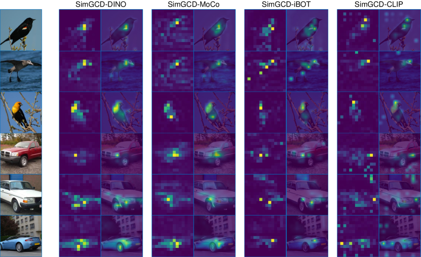
Figure 10: Attention map of class tokens on CUB (first three rows) and StanfordCars (last three rows) datasets. Each row displays the attention areas and attention maps for each image of SimGCD [40] with different backbone models.

It can be seen that different backbone models focus on different areas and they lack attention to more detailed and discriminative regions, making it challenging to distinguish visually similar categories. We argue that this is due to the model being trained solely on visual information from the dataset, making it challenging to generalize well to visually similar classes. Though visually similar, their text information tends to be different, promoting us to introduce text information into the task. In the meanwhile, the potential of current GCD methods heavily relies on the generalization ability of pre-trained models, prompting us to select a more robust and realistic pre-training model. As a large-scale model, CLIP shows strong generalization ability on downstream tasks and strong multi-modal potential due to its image-text contrastive training. Thus introducing CLIP into the GCD task not only enhances the basic class generalization ability but also builds a bridge to use use text information.

Appendix 0.F Qualitative Results

0.F.1 Cluster results of GET

As shown in Fig. 11, we present the comparative cluster accuracy between our multi-modal approach and previous single-modal methods on some visually similar classes in CUB datasets. It is worth noting that relying solely on visual information, even with a powerful CLIP backbone, the previous method (SimGCD-CLIP) still struggles to differentiate some categories, resulting in empty clusters. However, leveraging the rich and discriminative text information of categories, our GET achieves more accurate classification results on CUB without any empty clusters across all categories, demonstrating the importance of multi-modal information in the GCD task. Furthermore, we showcase the clustering results of SimGCD-CLIP (see in Fig. 14) and our GET  (see in Fig. 15) for the 170th class, “Mourning Warbler”, in the CUB dataset. SimGCD-CLIP relies solely on visual information to categorize birds based on shape and posture, the model categorizes many visually similar samples as “Mourning Warbler”. Our approach, by incorporating text information, enhances the model’s discriminative ability and correctly identifies all instances of the “Mourning Warbler” class, achieving 100% classification accuracy for this visually challenging category.

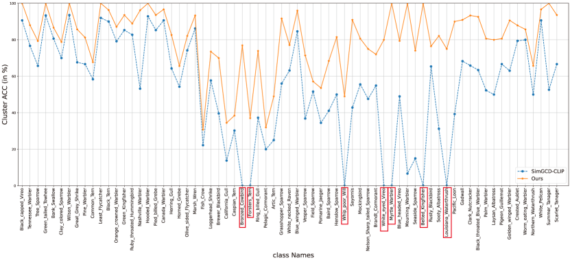
Figure 11: Cluster accuracy of SimGCD-CLIP and our GET on some visually similar classes in CUB datasets. GCD methods relying solely on a single visual modality result in empty clusters(highlighted by red boxes); Our multi-modal approach GET avoids empty clusters and achieves higher classification accuracy.

0.F.2 Attention map visualization of GET

We visualize the attention map of class tokens in Fig. 12. Compared to SimGCD-CLIP, our approach additionally focuses on the feather texture of birds, which is crucial for distinguishing visually similar fine-grained bird species. With the assistance of text information, the attention maps of our visual branch become more refined, focusing on more discriminative regions.

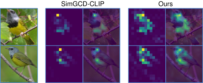
Figure 12: Attention map visualization of class tokens.

0.F.3 The t-SNE visualization

We randomly sample 20 classes from the 200 classes in the CUB dataset and perform the t-SNE projections of visual and text features. As shown in Fig. 13, both visual and text features of our method exhibit clear and compacter clusters.

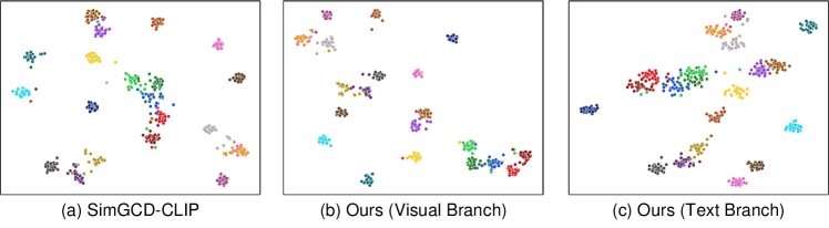
Figure 13: The t-SNE visualization of SimGCD-CLIP and our GET on CUB dataset.

Appendix 0.G Broader Impact and Limitations

Our approach introduces text information into the GCD task through the text embedding synthesizer module, extending the GCD to a multi-modal paradigm. Our method achieves state-of-the-art performance on all benchmark datasets and demonstrates the generalizability of TES in both parameterized and non-parameterized GCD methods. Our dual-branch multi-modal joint training framework with a cross-modal instance consistency objective provides an effective approach for leveraging multimodal information. A limitation of our approach is that we treat visual and text information as equally important. In fact, some samples may have richer and more discriminative visual information than textual information, and vice versa. A more appropriate approach might involve enabling the model to adaptively leverage multimodal information, autonomously assessing which modality’s information is more crucial. We will delve deeper into this aspect in our future work.

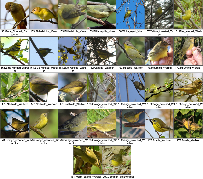
Figure 14: SimGCD-CLIP cluster results visualization for class “Mourning Warbler” in CUB dataset. SimGCD-CLIP categorizes birds based on shape and posture and incorrectly identifies many visually similar categories, resulting in a clustering accuracy of 6.7% for class “Mourning Warbler”.

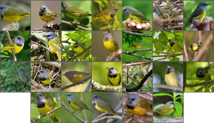
Figure 15: Cluster results visualization for class “Mourning Warbler” in CUB dataset of our GET. Our method uses multi-model information, achieving 100% classification accuracy for this visually challenging category.

References

- [1] Assran, M., Caron, M., Misra, I., Bojanowski, P., Bordes, F., Vincent, P., Joulin, A., Rabbat, M., Ballas, N.: Masked siamese networks for label-efficient learning. In: European Conference on Computer Vision. pp. 456–473. Springer (2022)
- [2] Cao, K., Brbic, M., Leskovec, J.: Open-world semi-supervised learning. In: International Conference on Learning Representations (2022), https://openreview.net/forum?id=O-r8LOR-CCA
- [3] Caron, M., Misra, I., Mairal, J., Goyal, P., Bojanowski, P., Joulin, A.: Unsupervised learning of visual features by contrasting cluster assignments. Advances in neural information processing systems 33, 9912–9924 (2020)
- [4] Caron, M., Touvron, H., Misra, I., Jégou, H., Mairal, J., Bojanowski, P., Joulin, A.: Emerging properties in self-supervised vision transformers. In: Proceedings of the IEEE/CVF international conference on computer vision. pp. 9650–9660 (2021)
- [5] Chen, F.L., Zhang, D.Z., Han, M.L., Chen, X.Y., Shi, J., Xu, S., Xu, B.: Vlp: A survey on vision-language pre-training. Machine Intelligence Research 20(1), 38–56 (2023)
- [6] Chen, X., Xie, S., He, K.: An empirical study of training self-supervised vision transformers (2021)
- [7] Chen, Y.C., Li, L., Yu, L., El Kholy, A., Ahmed, F., Gan, Z., Cheng, Y., Liu, J.: Uniter: Universal image-text representation learning. In: European conference on computer vision. pp. 104–120. Springer (2020)
- [8] Deng, J., Dong, W., Socher, R., Li, L.J., Li, K., Fei-Fei, L.: Imagenet: A large-scale hierarchical image database. In: CVPR (2009)
- [9] Dosovitskiy, A., Beyer, L., Kolesnikov, A., Weissenborn, D., Zhai, X., Unterthiner, T., Dehghani, M., Minderer, M., Heigold, G., Gelly, S., Uszkoreit, J., Houlsby, N.: An image is worth 16x16 words: Transformers for image recognition at scale. In: International Conference on Learning Representations (2021), https://openreview.net/forum?id=YicbFdNTTy
- [10] Du, Y., Liu, Z., Li, J., Zhao, W.X.: A survey of vision-language pre-trained models. arXiv preprint arXiv:2202.10936 (2022)
- [11] Fini, E., Sangineto, E., Lathuiliere, S., Zhong, Z., Nabi, M., Ricci, E.: A unified objective for novel class discovery. In: Proceedings of the IEEE/CVF International Conference on Computer Vision. pp. 9284–9292 (2021)
- [12] Gao, P., Geng, S., Zhang, R., Ma, T., Fang, R., Zhang, Y., Li, H., Qiao, Y.: Clip-adapter: Better vision-language models with feature adapters. arXiv preprint arXiv:2110.04544 (2021)
- [13] Han, K., Rebuffi, S.A., Ehrhardt, S., Vedaldi, A., Zisserman, A.: Automatically discovering and learning new visual categories with ranking statistics. In: International Conference on Learning Representations (ICLR) (2020)
- [14] Han, K., Vedaldi, A., Zisserman, A.: Learning to discover novel visual categories via deep transfer clustering. In: Proceedings of the IEEE/CVF International Conference on Computer Vision. pp. 8401–8409 (2019)
- [15] Hendrycks, D., Basart, S., Mu, N., Kadavath, S., Wang, F., Dorundo, E., Desai, R., Zhu, T., Parajuli, S., Guo, M., et al.: The many faces of robustness: A critical analysis of out-of-distribution generalization. In: Proceedings of the IEEE/CVF International Conference on Computer Vision. pp. 8340–8349 (2021)
- [16] Hsu, Y.C., Lv, Z., Kira, Z.: Learning to cluster in order to transfer across domains and tasks. In: International Conference on Learning Representations (2018)
- [17] Jia, C., Yang, Y., Xia, Y., Chen, Y.T., Parekh, Z., Pham, H., Le, Q., Sung, Y.H., Li, Z., Duerig, T.: Scaling up visual and vision-language representation learning with noisy text supervision. In: International conference on machine learning. pp. 4904–4916. PMLR (2021)
- [18] Khosla, P., Teterwak, P., Wang, C., Sarna, A., Tian, Y., Isola, P., Maschinot, A., Liu, C., Krishnan, D.: Supervised contrastive learning. Advances in neural information processing systems 33, 18661–18673 (2020)
- [19] Krause, J., Stark, M., Deng, J., Fei-Fei, L.: 3d object representations for fine-grained categorization. In: 4th International IEEE Workshop on 3D Representation and Recognition (3dRR-13) (2013)
- [20] Krizhevsky, A., Hinton, G.: Learning multiple layers of features from tiny images. Technical report (2009)
- [21] Krizhevsky, A., Sutskever, I., Hinton, G.E.: Imagenet classification with deep convolutional neural networks. Communications of the ACM 60(6), 84–90 (2017)
- [22] Kuhn, H.W.: The hungarian method for the assignment problem. Naval research logistics quarterly (1955)
- [23] Li, J., Selvaraju, R., Gotmare, A., Joty, S., Xiong, C., Hoi, S.C.H.: Align before fuse: Vision and language representation learning with momentum distillation. Advances in neural information processing systems 34, 9694–9705 (2021)
- [24] Li, L.H., Yatskar, M., Yin, D., Hsieh, C.J., Chang, K.W.: Visualbert: A simple and performant baseline for vision and language. arXiv preprint arXiv:1908.03557 (2019)
- [25] Lu, J., Batra, D., Parikh, D., Lee, S.: Vilbert: Pretraining task-agnostic visiolinguistic representations for vision-and-language tasks. Advances in neural information processing systems 32 (2019)
- [26] MacQueen, J., et al.: Some methods for classification and analysis of multivariate observations. In: Proceedings of the fifth Berkeley symposium on mathematical statistics and probability. vol. 1, pp. 281–297. Oakland, CA, USA (1967)
- [27] Maji, S., Rahtu, E., Kannala, J., Blaschko, M., Vedaldi, A.: Fine-grained visual classification of aircraft. arXiv preprint arXiv:1306.5151 (2013)
- [28] Merullo, J., Castricato, L., Eickhoff, C., Pavlick, E.: Linearly mapping from image to text space. arXiv preprint arXiv:2209.15162 (2022)
- [29] Ouldnoughi, R., Kuo, C.W., Kira, Z.: Clip-gcd: Simple language guided generalized category discovery. arXiv preprint arXiv:2305.10420 (2023)
- [30] Pu, N., Zhong, Z., Sebe, N.: Dynamic conceptional contrastive learning for generalized category discovery. In: Proceedings of the IEEE/CVF Conference on Computer Vision and Pattern Recognition. pp. 7579–7588 (2023)
- [31] Pu, N., Zhong, Z., Sebe, N.: Dynamic conceptional contrastive learning for generalized category discovery. In: Proceedings of the IEEE/CVF Conference on Computer Vision and Pattern Recognition (CVPR). pp. 7579–7588 (June 2023)
- [32] Radford, A., Kim, J.W., Hallacy, C., Ramesh, A., Goh, G., Agarwal, S., Sastry, G., Askell, A., Mishkin, P., Clark, J., et al.: Learning transferable visual models from natural language supervision. In: International conference on machine learning. pp. 8748–8763. PMLR (2021)
- [33] Shannon, C.E.: A mathematical theory of communication. The Bell system technical journal 27(3), 379–423 (1948)
- [34] Tan, H., Bansal, M.: Lxmert: Learning cross-modality encoder representations from transformers. arXiv preprint arXiv:1908.07490 (2019)
- [35] Tan, K.C., Liu, Y., Ambrose, B., Tulig, M., Belongie, S.: The herbarium challenge 2019 dataset. In: Workshop on Fine-Grained Visual Categorization (2019)
- [36] Vaze, S., Han, K., Vedaldi, A., Zisserman, A.: Generalized category discovery. In: Proceedings of the IEEE/CVF Conference on Computer Vision and Pattern Recognition. pp. 7492–7501 (2022)
- [37] Vaze, S., Han, K., Vedaldi, A., Zisserman, A.: Open-set recognition: a good closed-set classifier is all you need? In: International Conference on Learning Representations (2022)
- [38] Vaze, S., Vedaldi, A., Zisserman, A.: No representation rules them all in category discovery. Advances in Neural Information Processing Systems 37 (2023)
- [39] Wah, C., Branson, S., Welinder, P., Perona, P., Belongie, S.: The Caltech-UCSD Birds-200-2011 Dataset. Tech. Rep. CNS-TR-2011-001, California Institute of Technology (2011)
- [40] Wen, X., Zhao, B., Qi, X.: Parametric classification for generalized category discovery: A baseline study. In: Proceedings of the IEEE/CVF International Conference on Computer Vision. pp. 16590–16600 (2023)
- [41] Wu, S., Zhang, W., Jin, S., Liu, W., Loy, C.C.: Aligning bag of regions for open-vocabulary object detection. In: CVPR (2023)
- [42] Wu, Z., Xiong, Y., Yu, S.X., Lin, D.: Unsupervised feature learning via non-parametric instance discrimination. In: Proceedings of the IEEE conference on computer vision and pattern recognition. pp. 3733–3742 (2018)
- [43] Zhang, S., Khan, S., Shen, Z., Naseer, M., Chen, G., Khan, F.S.: Promptcal: Contrastive affinity learning via auxiliary prompts for generalized novel category discovery. In: Proceedings of the IEEE/CVF Conference on Computer Vision and Pattern Recognition. pp. 3479–3488 (2023)
- [44] Zhao, B., Han, K.: Novel visual category discovery with dual ranking statistics and mutual knowledge distillation. In: Conference on Neural Information Processing Systems (NeurIPS) (2021)
- [45] Zhao, B., Wen, X., Han, K.: Learning semi-supervised gaussian mixture models for generalized category discovery. arXiv preprint arXiv:2305.06144 (2023)
- [46] Zhao, B., Wen, X., Han, K.: Learning semi-supervised gaussian mixture models for generalized category discovery. In: Proceedings of the IEEE/CVF International Conference on Computer Vision (ICCV). pp. 16623–16633 (October 2023)
- [47] Zhou, J., Wei, C., Wang, H., Shen, W., Xie, C., Yuille, A., Kong, T.: ibot: Image bert pre-training with online tokenizer. arXiv preprint arXiv:2111.07832 (2021)