Inference for non-probability samples using the calibration approach for quantiles

Abstract

Non-probability survey samples are examples of data sources that have become increasingly popular in recent years, also in official statistics. However, statistical inference based on non-probability samples is much more difficult because they are biased and are not representative of the target population [75]. In this paper we consider a method of joint calibration for totals [55] and quantiles [59] and use the proposed approach to extend existing inference methods for non-probability samples, such as inverse probability weighting, mass imputation and doubly robust estimators. By including quantile information in the estimation process non-linear relationships between the target and auxiliary variables can be approximated the way it is done in step-wise (constant) regression. Our simulation study has demonstrated that the estimators in question are more robust against model mis-specification and, as a result, help to reduce bias and improve estimation efficiency. Variance estimation for our proposed approach is also discussed. We show that existing inference methods can be used and that the resulting confidence intervals are at nominal levels. Finally, we applied the proposed methods to estimate the share of vacancies aimed at Ukrainian workers in Poland using an integrated set of administrative and survey data about job vacancies. The proposed approaches have been implemented in two R packages (nonprobsvy and jointCalib), which were used to conduct the simulation and empirical study.

Key Words: inverse probability weighting, doubly robust, quantiles, mass imputation, job vacancy survey.

1 Introduction

In official statistics, information about the target population and its characteristics is mainly collected through probability surveys or is obtained from administrative registers, which cover all (or nearly all) units of the population. However, owing to increasing non-response rates, particularly unit non-response and non-contact (resulting from the growing respondent burden), as well as rising costs of surveys conducted by National Statistical Institutes (NSIs), non-statistical data sources are becoming more popular [42, 41]. Non-probability surveys, such as opt-in web panels, social media, scanner data, mobile phone data or voluntary register data, are currently being explored for use in the production of official statistics [53, 52]. Since the selection mechanism in these sources is unknown, standard design-based inference methods cannot be directly applied.

To address this problem, several approaches based on inverse probability weighting (IPW), mass imputation (MI) and doubly robust (DR) estimators have been proposed for two main scenarios: 1) population-level data are available, either in the form of unit-level data (e.g. from a register covering the whole population) or known population totals/means, and 2) only survey data are available as a source of information about the target population [57, 75, cf. ]. Most approaches assume that population data are used to reduce the bias of non-probability sampling by reweighting to reproduce known population totals/means, by modelling $E(Y|\boldsymbol{X})$ using various techniques or combining both approaches (cf. doubly robust estimators, cf. [49]; multilevel regression and post-stratification - MRP also called Mister-P, cf. [58]). Most of these methods rely on a limited number of moments of continuous or count data, with some exceptions. For example, non-parametric approaches based on nearest neighbours (NN), such as those discussed by Yang, Kim and Hwang (yang2021integration) or kernel density estimation (KDE) described by Chen, Yang and Kim (chen_nonparametric_2022) have also been proposed. In general, the standard approach, such as IPW, seems to be limited, although surveys and register data contain continuous or count data which can be used to account for distribution mismatches.

In this paper, we extend existing methods to account for distribution differences through the use of calibration for quantiles. We use the idea of survey calibration for quantiles described by [59] and propose a joint calibration approach to quantiles and totals using the paradigm proposed by [55]. Finally, we adapt this concept to MI, IPW and DR estimators. Our contribution can be summarised as follows:

• we extend the calibration paradigm to jointly account for totals/means and quantiles in non-probability samples. This method can be further extended to model-assisted and model-based calibration approaches proposed by [47, 74, 46];

• we extend IPW, MI and DR estimators for non-probability samples to account not only for totals/means but also for the distribution of auxiliary variables in the form of a set of quantiles;

• we show that existing inference methods hold for the proposed techniques;

• adding information on quantiles is equivalent to using step-wise (constant) regression, which can be used to approximate a non-linear relationship through a linear model, making MI, IPW and DR more robust to model mis-specification, and consequently, decreasing the bias and improving efficiency of estimation.

In this paper we generally follow the notation used by [75]. The paper has the following structure. In Section 2 we introduce the basic setup: the notation and a short description of calibration for totals and quantiles separately. In Section 3 we describe the procedure of joint calibration of totals and quantiles. Section 4 describes an extension for the prediction approach, in particular mass imputation. Section 5 deals with an extension to the inverse probability weighting estimator and in Section 6 we propose an extension to doubly robust estimators. Finally, Section 7 contains results of a simulation study and Section 8 summarises results from a study in which the proposed approach was applied to combined data from a job vacancy survey and online vacancies. The paper ends with conclusions and identifies research problems that require further investigation.

2 Basic setup

2.1 Notation

Let $U=\{1,...,N\}$ denote the target population consisting of $N$ labelled units. Each unit $k$ has an associated vector of auxiliary variables $\boldsymbol{x}$ and the target variable $y$, with their corresponding values $\boldsymbol{x}_{k}$ and $y_{k}$, respectively. Let $\{(y_{k},\boldsymbol{x}_{k}),k\in S_{A}\}$ be a dataset of a non-probability sample of size $n_{A}$ and $\{(\boldsymbol{x}_{k},d_{k}^{B}),k\in S_{B}\}$ – a dataset of a probability sample of size $n_{B}$. Only information about auxiliary variables $\boldsymbol{x}$ is found in both datasets and $d_{k}^{B}=1/\pi_{k}^{B}$ are design-based weights assigned to each unit in the sample. Table 2.1 summarises the setup, which contains no overlap.

Table 2.1: A setup with two data sources

Sample	ID	Sample weight $d=\pi^{-1}$	Covariates $\boldsymbol{x}$	Study variable $y$
Non-probability sample ($S_{A})$	1	?	$\checkmark$	$\checkmark$
	$\vdots$	?	$\vdots$	$\vdots$
	$n_{A}$	?	$\checkmark$	$\checkmark$
Probability sample ($S_{B}$)	1	$\checkmark$	$\checkmark$	?
	$\vdots$	$\vdots$	$\vdots$	?
	$n_{B}$	$\checkmark$	$\checkmark$	?

Let $R_{k}=I(k\in S_{A})$ be the indicator variable showing that unit $k$ is included in the non-probability sample $S_{A}$, which is defined for all units in the population $U$. Let $\pi_{k}^{A}=P(R_{k}=1|\boldsymbol{x}_{k})$ for $k=1,...,N$ be their propensity scores. For $\pi_{k}^{A}$ we can assume a parametric model $\pi(\boldsymbol{x}_{k},\boldsymbol{\gamma})$ (e.g. logistic regression) with unknown model parameters $\boldsymbol{\gamma}$.

The goal is to estimate a finite population total $\tau_{y}=\sum_{k\in U}y_{k}$ or the mean $\bar{\tau}_{y}=\tau_{y}/N$ of the variable of interest $y$. In probability surveys (assuming that $y_{k}$ are known), the Horvitz-Thompson is the well-known estimator of a finite population total, which is expressed as $\hat{\tau}_{y\pi}=\sum_{k\in s}{d_{k}y_{k}}$, where $s$ denotes a probability sample of size $n$, $d_{k}=1/\pi_{k}$ is a design weight and $\pi_{k}$ is the first-order inclusion probability of the $i$-th element of the population $U$. This estimator is unbiased for $\tau_{y}$ i.e. $E\left(\hat{\tau}_{y\pi}\right)=\tau_{y}$. However, a different approach should be applied for non-probability surveys, as $\pi_{k}^{A}$ are unknown and have to be estimated.

Throughout the paper we follow standard assumptions for inference based on non-probability samples, i.e: (A1) conditional independence of $R_{k}$ and $y_{k}$ given $\boldsymbol{x}_{k}$; (A2) all units in the target population have non-zero propensity scores $\pi_{k}^{A}>0$; and (A3) $R_{1},...,R_{N}$ are independent given auxiliary variables $(\boldsymbol{x}_{1},...,\boldsymbol{x}_{N})$.

In order to present our approach, we briefly introduce the notation used for calibration of totals/means, quantiles and joint calibration in the context of non-probability surveys.

2.2 Calibration estimator for a total and a mean

Let $\boldsymbol{x}_{k}^{\circ}$ be a $J_{1}$-dimensional vector of auxiliary variables (benchmark variables) for which $\tau_{\boldsymbol{x}}=\sum_{k\in U}\boldsymbol{x}_{k}^{\circ}=\left(\sum_{k\in U}x_{k1},\ldots,\sum_{k\in U}x_{kJ_{1}}\right)^{T}$ is assumed to be known. The main idea of calibration for non-probability samples is to look for new calibration weights $w_{k}^{A}$ that are as close as possible to original weights $d_{k}^{A}$ (in most cases it is assumed that $d_{k}^{A}=1$ or $d_{k}^{A}=N/n_{A}$) and reproduce known population totals $\tau_{\boldsymbol{x}}$ exactly. In other words, in order to find new calibration weights $w_{k}^{A}$ we have to minimise a distance function $D\left(\boldsymbol{d},\boldsymbol{v}\right)=\sum_{k\in S_{A}}d_{k}^{A}\hskip 2.0ptG\left(\frac{v_{k}^{A}}{d_{k}^{A}}\right)\to\textrm{min}$ to fulfil calibration equations $\sum_{k\in S_{A}}v_{k}^{A}\boldsymbol{x}_{k}^{\circ}=\sum_{k\in U}\boldsymbol{x}_{k}^{\circ}$, where $\boldsymbol{d}=\left(d_{1}^{A},\ldots,d_{n_{A}}^{A}\right)^{T}$, $\boldsymbol{v}=\left(v_{1}^{A},\ldots,v_{n_{A}}^{A}\right)^{T}$ and $G\left(\cdot\right)$ is a function that must satisfy some regularity conditions: $G\left(\cdot\right)$ is strictly convex and twice continuously differentiable, $G\left(\cdot\right)\geq 0$, $G\left(1\right)=0$, $G^{\prime}\left(1\right)=0$ and $G^{\prime\prime}\left(1\right)=1$. Examples of $G\left(\cdot\right)$ functions are given by [55]. For instance, if $G\left(x\right)=\frac{\left(x-1\right)^{2}}{2}$, then using the method of Lagrange multipliers the final calibration weights $w_{k}^{A}$ can be expressed as $w_{k}^{A}=d_{k}^{A}+d_{k}^{A}\left(\tau_{\boldsymbol{x}}-\hat{\tau}_{\boldsymbol{x}\pi}\right)^{T}\left(\sum_{j\in S_{A}}d_{j}^{A}\boldsymbol{x}_{j}^{\circ}\boldsymbol{x}_{j}^{\circ T}\right)^{-1}\boldsymbol{x}_{k}^{\circ}$. It is worth adding that in order to avoid negative or large $w_{k}^{A}$ weights in the process of minimising the $D\left(\cdot\right)$ function, one can consider some boundary constraints $L\leq\frac{w_{k}^{A}}{d_{k}^{A}}\leq U$, where $\ 0\leq L\leq 1\leq U,\ k=1,\ldots,n_{A}$. The final calibration estimator of a population total $\tau_{y}$ based on a non-probability sample can be expressed as $\hat{\tau}_{y\boldsymbol{x}^{\circ}}=\sum_{k\in S_{A}}w_{k}^{A}y_{k}$, where $w_{k}^{A}$ are calibration weights obtained using a specific $G\left(\cdot\right)$ function.

2.3 Calibration estimator for a quantile

[59] considered the estimation of quantiles using the calibration approach in a way very similar to what [55] proposed for a finite population total $\tau_{y}$. By analogy, in their approach it is not necessary to know values of all auxiliary variables for all units in the population. It is enough to know the corresponding quantiles for the benchmark variables. Below we briefly discuss the problem of finding calibration weights under this setup by adjusting this approach to a non-probability sample $S_{A}$.

We want to estimate a quantile $Q_{y,\alpha}$ of order $\alpha\in\left(0,1\right)$ of the variable of interest $y$, which can be expressed as $Q_{y,\alpha}=\mathrm{inf}\left\{t\left|F_{y}\left(t\right)\geq\alpha\right.\right\}$, where $F_{y}\left(t\right)=N^{-1}\sum_{k\in U}H\left(t-y_{k}\right)$ and the Heavyside function is given by

$$H\left(t-y_{k}\right)=\left\{\begin{array}[]{ll}1,&\ t\geq y_{k},\\ 0,&\ t<y_{k}.\\ \end{array}\right.$$ (1)

We assume that $\boldsymbol{Q}_{\boldsymbol{x},\alpha}=\left(Q_{x_{1},\alpha},\ldots,Q_{x_{J_{2}},\alpha}\right)^{T}$ is a vector of known population quantiles of order $\alpha$ for a vector of auxiliary variables $\boldsymbol{x}_{k}^{*}$, where $\alpha\in\left(0,1\right)$ and $\boldsymbol{x}_{k}^{*}$ is a $J_{2}$-dimensional vector of auxiliary variables. It is worth noting that, in general, the numbers $J_{1}$ and $J_{2}$ of auxiliary variables may be different. It may happen that for a specific auxiliary variable its population total and the corresponding quantile of order $\alpha$ will be known. However, in most cases quantiles will be known for continuous auxiliary variables, unlike totals, which will generally be known for categorical variables. In order to find new calibration weights $w_{k}^{A}$ that reproduce known population quantiles in a vector $Q_{\boldsymbol{x},\alpha}$, an interpolated distribution function estimator of $F_{y}\left(t\right)$ is defined as $\hat{F}_{y,cal}(t)=\frac{\sum_{k\in S_{A}}w_{k}^{A}H_{y,S_{A}}\left(t,y_{k}\right)}{\sum_{k\in S_{A}}w_{k}^{A}}$, where the Heavyside function in formula (1) is replaced by the modified function $H_{y,S_{A}}\left(t,y_{k}\right)$ given by

$$H_{y,S_{A}}\left(t,y_{k}\right)=\left\{\begin{array}[]{ll}1,&y_{k}\leqslant L_{y,S_{A}}(t),\\ \beta_{y,S_{A}}\left(t\right),&y_{k}=U_{y,S_{A}}\left(t\right),\\ 0,&y_{k}>U_{y,S_{A}}\left(t\right),\end{array}\right.$$ (2)

where appropriate parameters are defined as $L_{y,S_{A}}\left(t\right)=\max\left\{\left\{y_{k},k\in S_{A}\mid y_{k}\leqslant t\right\}\cup\{-\infty\}\right\}$, $U_{y,S_{A}}\left(t\right)=\min\left\{\left\{y_{k},k\in S_{A}\mid y_{k}>t\right\}\cup\{\infty\}\right\}$ and $\beta_{y,S_{A}}\left(t\right)=\frac{t-L_{y,S_{A}}\left(t\right)}{U_{y,S_{A}}\left(t\right)-L_{y,S_{A}}\left(t\right)}$ for $k=1,\ldots,n_{A}$, $t\in\mathbb{R}$. From a practical point of view a smooth approximation to the step function, based on the logistic function can be used i.e. $H\left(x\right)\approx\frac{1}{2}+\frac{1}{2}\tanh{kx}=(1+e^{-2kx})^{-1}$, where a larger value of $k$ corresponds to a sharper transition at $x=0$.

A calibration estimator of quantile $Q_{y,\alpha}$ of order $\alpha$ for variable $y$ is defined as $\hat{Q}_{y,cal,\alpha}=\hat{F}_{y,cal}^{-1}(\alpha)$, where a vector $\boldsymbol{w}=\left(w_{1}^{A},\ldots,w_{n_{A}}^{A}\right)^{T}$ is a solution of an optimization problem $D\left(\boldsymbol{d},\boldsymbol{v}\right)=\sum_{k\in S_{A}}d_{k}^{A}\hskip 2.0ptG\left(\frac{v_{k}^{A}}{d_{k}^{A}}\right)\to\textrm{min}$ subject to the calibration constraints $\sum_{k\in S_{A}}v_{k}^{A}=N$ and $\hat{\boldsymbol{Q}}_{\boldsymbol{x},cal,\alpha}=\left(\hat{Q}_{x_{1},cal,\alpha},\ldots,\hat{Q}_{x_{J_{2}},cal,\alpha}\right)^{T}=\boldsymbol{Q}_{\boldsymbol{x},\alpha}$ or equivalently $\hat{F}_{x_{j},cal}\left(Q_{x_{j},\alpha}\right)=\alpha$, where $j=1,\ldots,J_{2}$.

As in the previous case, if $G\left(x\right)=\frac{\left(x-1\right)^{2}}{2}$, then, using the method of Lagrange multipliers, the final weights $w_{k}^{A}$ can be expressed as $w_{k}^{A}=d_{k}^{A}+d_{k}^{A}\left(\mathbf{T_{a}}-\sum_{k\in S_{A}}{d_{k}^{A}\boldsymbol{a}_{k}}\right)^{T}\left(\sum_{j\in S_{A}}{d_{j}^{A}}\boldsymbol{a}_{j}\boldsymbol{a}_{j}^{T}\right)^{-1}\boldsymbol{a}_{k}$, where $\mathbf{T_{a}}=\left(N,\alpha,\ldots,\alpha\right)^{T}$ and the elements of $\boldsymbol{a}_{k}=\left(1,a_{k1},\ldots,a_{kJ_{2}}\right)^{T}$ are given by

$$a_{kj}=\left\{\begin{array}[]{lll}N^{-1},&\quad x_{kj}\leq L_{x_{j},S_{A}}\left(Q_{x_{j},\alpha}\right),\\ N^{-1}\beta_{x_{j},S_{A}}\left(Q_{x_{j},\alpha}\right),&\quad x_{kj}=U_{x_{j},S_{A}}\left(Q_{x_{j},\alpha}\right),\\ 0,&\quad x_{kj}>U_{x_{j},S_{A}}\left(Q_{x_{j},\alpha}\right),\\ \end{array}\right.$$ (3)

with $j=1,\ldots,J_{2}$.

Assuming that $y_{1}\leq y_{2}\ldots\leq y_{n_{A}}$, it can be shown that if there exists $l\!\in\!\!{\left\{1,\ldots,n_{A}-1\right\}}$ such that $\hat{F}_{y,cal}\left(y_{p}\right)\leq\alpha$, $\hat{F}_{y,cal}\left(y_{p+1}\right)>\alpha$ and $\hat{F}_{y,cal}$ is invertible at point $\hat{Q}_{y,cal,\alpha}$, then the calibration estimator $\hat{Q}_{y,cal,\alpha}$ of quantile $Q_{y,\alpha}$ of order $\alpha\in\left(0,1\right)$ can be expressed as $\hat{Q}_{y,cal,\alpha}=y_{l}+\frac{N\alpha-\sum_{k=1}^{l}{w_{k}^{A}}}{w_{l+1}^{A}}\left(y_{l+1}-y_{l}\right)$.

In the method described above it is assumed that a known population quantile is reproduced for a set of auxiliary variables, i.e. that the process of calibration is based on a particular quantile (of order $\alpha$). For instance, it could be the median $\alpha=0.5$. Nothing stands in the way of searching for calibration weights which reproduce population quantiles (for example quartiles) for a chosen set of auxiliary variables.

3 Joint calibration for totals and quantiles

First, we propose what we call joint calibration, which relies on auxiliary information about totals of $\boldsymbol{x}_{k}^{\circ}$ and quantiles of $\boldsymbol{x}_{k}^{*}$. After applying joint calibration, the resulting calibrated weights $w_{k}^{A}$ should make it possible to obtain known population totals and quantiles of auxiliary variables simultaneously.

Let us assume that we are interested in estimating a population total $\tau_{y}$ and/or quantile $Q_{y,\alpha}$ of order $\alpha$, where $\alpha\in\left(0,1\right)$ for the variable of interest $y$. Let $\boldsymbol{x}_{k}=\left(\begin{smallmatrix}\boldsymbol{x}_{k}^{\circ}\\ 1\\ \boldsymbol{x}_{k}^{*}\end{smallmatrix}\right)$ be a $J+1$-dimensional vector of auxiliary variables, where $J=J_{1}+J_{2}$. We assume that for $J_{1}$ variables a vector of population totals $\tau_{\boldsymbol{x}}$ and for $J_{2}$ variables a vector $\boldsymbol{Q}_{\boldsymbol{x},\alpha}$ of population quantiles is known respectively. In practice, it may happen that for the same auxiliary variable we know its population total and its quantile. It is not necessary that the complete auxiliary information described by the vector $\boldsymbol{x}_{k}$ should be known for all $k\in U$; however, for some auxiliary variables unit-population data would be necessary, because accurate quantiles are not likely to be known from other sources [71].

In our joint approach we are looking for a vector $\boldsymbol{w}=\left(w_{1}^{A},\ldots,w_{n}^{A}\right)^{T}$ which is a solution to the optimization problem $D\left(\boldsymbol{d},\boldsymbol{v}\right)=\sum_{k\in S_{A}}d_{k}^{A}\hskip 2.0ptG\left(\frac{v_{k}^{A}}{d_{k}^{A}}\right)\to\textrm{min}$ subject to the calibration constraints $\sum_{k\in S{{}_{A}}}v_{k}^{A}=N$, $\sum_{k\in S_{A}}v_{k}^{A}\boldsymbol{x}_{k}^{\circ}=\tau_{\boldsymbol{x}}$ and $\hat{\boldsymbol{Q}}_{\boldsymbol{x},cal,\alpha}=\boldsymbol{Q}_{\boldsymbol{x},\alpha}$. In general, $J+1$ calibration equations have to be fulfilled. Alternatively, calibration equations can be expressed as $\sum_{k\in S_{A}}v_{k}^{A}\boldsymbol{x}_{k}^{\circ}=\tau_{\boldsymbol{x}}$ and $\sum_{k\in S_{A}}v_{k}^{A}\boldsymbol{a}_{k}=\mathbf{T_{a}}$ with possible boundary constraints on calibration weights.

Assuming a quadratic metric $D\left(\cdot\right)$, which is based on $G\left(x\right)=\frac{\left(x-1\right)^{2}}{2}$ function, an explicit solution to the above optimisation problem can be derived. This solution is similar to the calibration weights for totals and quantiles. Let $\boldsymbol{h}_{\boldsymbol{x}}=\binom{\tau_{\boldsymbol{x}}}{\mathbf{T_{a}}}$ and $\hat{\boldsymbol{h}}_{\boldsymbol{x}}=\binom{\sum_{k\in S_{A}}d_{k}^{A}\boldsymbol{x}_{k}^{\circ}}{\sum_{k\in S_{A}}d_{k}^{A}\boldsymbol{a}_{k}}$. Then the vector of calibration weights $\boldsymbol{w}=\left(w_{1}^{A},\ldots,w_{n_{A}}^{A}\right)^{T}$ which solves the above optimisation problem satisfies the relation:

$$w_{k}^{A}=d_{k}^{A}+d_{k}^{A}\left(\boldsymbol{h}_{\boldsymbol{x}}-\hat{\boldsymbol{h}}_{\boldsymbol{x}}\right)^{T}\left(\sum_{j\in S_{A}}{d_{j}^{A}}\boldsymbol{x}_{j}\boldsymbol{x}_{j}^{T}\right)^{-1}\boldsymbol{x}_{k}.$$ (4)

Under this function, the calibration estimator using (4) is equivalent to a generalised linear regression estimator (GREG) given by

$$\hat{\tau}_{y\boldsymbol{x}}^{GREG}=\sum_{k\in S_{A}}d_{k}^{A}y_{k}+\left(\boldsymbol{h}_{x}-\hat{\boldsymbol{h}}_{x}\right)^{T}\hat{\boldsymbol{\beta}},$$

where

$$\hat{\boldsymbol{\beta}}=\begin{pmatrix}\hat{\boldsymbol{\beta}}^{\circ}\\ \hat{\boldsymbol{\beta}}^{*}\end{pmatrix}=\left(\sum_{k\in S_{A}}d_{k}^{A}\boldsymbol{x}_{k}\boldsymbol{x}_{k}^{T}\right)^{-1}\sum_{k\in S_{A}}d_{k}^{A}\boldsymbol{x}_{k}y_{k}=\begin{pmatrix}\sum_{k\in S_{A}}d_{k}^{A}\boldsymbol{x}_{k}^{\circ}\left(\boldsymbol{x}_{k}^{\circ}\right)^{T}\\ \sum_{k\in S_{A}}d_{k}^{A}\boldsymbol{a}_{k}\boldsymbol{a}_{k}^{T}\end{pmatrix}^{-1}\begin{pmatrix}\sum_{k\in S_{A}}d_{k}^{A}\boldsymbol{x}_{k}^{\circ}\\ \sum_{k\in S_{A}}d_{k}^{A}\boldsymbol{a}_{k}\end{pmatrix}y_{k}.$$

The vector of coefficients $\hat{\boldsymbol{\beta}}$ is decomposed into two vectors: $\hat{\boldsymbol{\beta}}^{\circ}$ refers to auxiliary variables $\boldsymbol{x}_{k}^{\circ}$ and $\hat{\boldsymbol{\beta}}^{*}$ refers to $\boldsymbol{x}_{k}^{*}$ through vector $\boldsymbol{a}_{k}$. Note that $\hat{\boldsymbol{\beta}}^{*}$ contains an intercept as vector $\boldsymbol{a}_{k}$ contains 1. Therefore, we assume that the relationship between auxiliary variables $\boldsymbol{x}_{k}^{\circ}$ and $\boldsymbol{x}_{k}^{*}$ through $\boldsymbol{a}_{k}$ is linear as in

$$\hat{y}_{k}=\left(\boldsymbol{x}_{k}^{\circ}\right)^{T}\hat{\boldsymbol{\beta}}^{\circ}+\boldsymbol{a}_{k}^{T}\hat{\boldsymbol{\beta}}^{*}.$$ (5)

This means that the proposed estimator is asymptotically design-unbiased if the relationship between $y$ and $\boldsymbol{x}$ is linear. In the next section we discuss how model (5) approximates non-linear relationships and thus can provide some robustness against such situations.

In our proposed method we assume that known population totals and known population quantiles are reproduced for a set of benchmark variables simultaneously. This approach can be easily extended by assuming that estimated totals or quantiles are reproduced for some auxiliary variables. Furthermore, this approach can be further extended to model-assisted calibration as proposed in [44, 45].

4 Extension to the prediction approach

4.1 Basic prediction approach

[57, 75] reviewed existing prediction approaches for non-probability samples, which can be summarised as follows. We assume the following semi-parametric model for a finite population, denoted as $\xi$:

$$E_{\xi}\left(y_{k}\mid\boldsymbol{x}_{k}^{\circ}\right)=m\left(\boldsymbol{x}^{\circ}_{k},\boldsymbol{\beta}^{\circ}\right)\text{, and }\quad V_{\xi}\left(y_{k}\mid\boldsymbol{x}^{\circ}_{k}\right)=v\left(\boldsymbol{x}^{\circ}_{k}\right)\sigma^{2},\quad k=1,2,\ldots,N\text{, }$$

where the mean function $m(\cdot,\cdot)$ and $v(\cdot)$ have known forms. Under assumption (A1) we have $E_{\xi}\left(y_{k}\mid\boldsymbol{x}^{\circ}_{k},R_{k}=1\right)=E_{\xi}\left(y_{k}\mid\boldsymbol{x}^{\circ}_{k}\right)$ and $V_{\xi}\left(y_{k}\mid\boldsymbol{x}^{\circ}_{k},R_{k}=1\right)=V_{\xi}\left(y_{k}\mid\boldsymbol{x}^{\circ}_{k}\right)$, which means that the population model holds for a non-probability sample $S_{A}$. For example, we can use generalized linear models (GLM) for $m(\cdot,\cdot)$.

[75] discussed two general forms of prediction estimators when either population data or a probability sample $S_{B}$ is available and mass imputation when non-probability $S_{A}$ and probability $S_{B}$ samples are used. Let $m_{k}=m(\boldsymbol{x}^{\circ}_{k},\boldsymbol{\beta}^{\circ})$ and $\hat{m}_{k}=m(\boldsymbol{x}^{\circ}_{k},\hat{\boldsymbol{\beta}}^{\circ})$ then two general estimators of the population mean $\hat{\bar{\tau}}$ are given by

$$\hat{\bar{\tau}}_{y1}=\frac{1}{N}\sum_{k\in U}\hat{m}_{k}\quad\text{ and }\quad\hat{\bar{\tau}}_{y2}=\frac{1}{N}\left\{\sum_{k\in S_{A}}y_{k}-\sum_{k\in S_{A}}\hat{m}_{k}+\sum_{k\in U}\hat{m}_{k}\right\}.$$ (6)

Under a linear model where $m(\boldsymbol{x}^{\circ}_{k},\boldsymbol{\beta}^{\circ})=(\boldsymbol{x}_{k}^{\circ})^{T}\boldsymbol{\beta}^{\circ}$, the two estimators given in (6) reduce to

$$\hat{\bar{\tau}}_{y_{1}}=\bar{\tau}_{\boldsymbol{x}^{\circ}}^{T}\hat{\boldsymbol{\beta}}^{\circ}\quad\text{ and }\quad\hat{\bar{\tau}}_{y_{2}}=\frac{n_{A}}{N}\left(\bar{y}_{A}-\bar{\tau}_{\boldsymbol{x}^{\circ}}^{T}\hat{\boldsymbol{\beta}^{\circ}}\right)+\bar{\tau}_{\boldsymbol{x}^{\circ}}^{T}\hat{\boldsymbol{\beta}^{\circ}},$$ (7)

where $\bar{\tau}_{\boldsymbol{x}^{\circ}}$ is the vector of the population means of the $\boldsymbol{x}^{\circ}$ variables and $\bar{y}_{A}$ is a non-probability sample mean. If information about auxiliary variables is available through probability sample $S_{B}$, we replace $\sum_{k\in U}\hat{m}_{k}$ with $\sum_{k\in S_{B}}d_{k}^{B}\hat{m}_{k}$ in (6) and $\bar{\tau}_{\boldsymbol{x}^{\circ}}$ with $\hat{\bar{\tau}}_{\boldsymbol{x}^{\circ}}=\hat{N}_{B}^{-1}\sum_{k\in S_{B}}d_{k}^{B}\boldsymbol{x}_{k}^{\circ}$ in (7) where $\hat{N}_{B}=\sum_{k\in S_{B}}d_{k}^{B}$.

When a mass imputation estimator is considered, inference is based on the following formula

$$\hat{\bar{\tau}}_{yMI}=\frac{1}{\hat{N}_{B}}\sum_{k\in S_{B}}d_{k}^{B}y_{k}^{*},$$ (8)

where $y_{k}^{*}$ is an imputed value of $y_{k}$. There are two main approaches to imputing $y_{k}$ in $S_{B}$: 1) deterministic regression imputation $y_{k}^{*}=(\boldsymbol{x}_{k}^{\circ})^{T}\hat{\boldsymbol{\beta}^{\circ}}$, and 2) sample matching, where each unit in $S_{B}$ is matched to units from $S_{A}$ based on $\boldsymbol{x}^{\circ}$.

Remark 1. [63] showed that asymptotic bias of estimator (8) is given by

$$E(\hat{\bar{\tau}}_{yMI}-\bar{\tau}_{y})\approx E\left(Cov_{N}\left(R\frac{N}{n_{B}},e^{*}\right)\right),$$

where $e^{*}=y_{k}-m_{k}$. The proposed approach will be asymptotically unbiased if the model $m(\boldsymbol{x},\boldsymbol{\beta})$ is correctly specified or could have lower bias if adding $\boldsymbol{x}_{k}^{*}$ through $\boldsymbol{a}_{k}$ improves the fit in comparison to a model which only uses $\boldsymbol{x}_{k}^{\circ}$. This is because the variance of $e^{*}$ can be smaller for a model that includes $\boldsymbol{a}_{k}$.

4.2 The proposed extension to the prediction approach

In our proposal we consider the same approach as in (5), i.e. we assume a generalised linear model for $m(\cdot,\cdot)$ given $\boldsymbol{x}_{k}^{\star}$ or $\boldsymbol{x}_{k}$, which contains both types of auxiliary variables. Thus, we can consider the following population models when linear regression is assumed:

• only $\boldsymbol{x}_{k}^{*}$ is used through $\boldsymbol{a}_{k}$ variables: $m(\boldsymbol{x}_{k}^{*},\boldsymbol{\beta}^{*})=m(\boldsymbol{a}_{k},\boldsymbol{\beta}^{*})=\boldsymbol{a}_{k}^{T}\boldsymbol{\beta}^{*}$,

• both $\boldsymbol{x}_{k}^{*}$ and $\boldsymbol{x}_{k}^{\circ}$ are used: $m(\boldsymbol{x}_{k},\boldsymbol{\beta})=(\boldsymbol{x}_{k}^{\circ})^{T}\boldsymbol{\beta}^{\circ}+\boldsymbol{a}_{k}^{T}\boldsymbol{\beta}^{*}$,

under the same assumptions (A1)–(A3) and requirements for the estimation of $\boldsymbol{\beta}$. Then, it is straightforward to estimate population mean $\hat{\bar{\tau}}$ based in (6) or (8). A small modification is required for (7) when linear regression is assumed:

$$\hat{\bar{\tau}}_{y_{1}} =\bar{\tau}^{T}_{\boldsymbol{x}}\hat{\boldsymbol{\beta}}=\bar{\tau}_{\boldsymbol{x}^{\circ}}^{T}\hat{\boldsymbol{\beta}}^{\circ}+\bar{\tau}_{\boldsymbol{a}}^{T}\hat{\boldsymbol{\beta}}^{*},$$ (9)

$$\hat{\bar{\tau}}_{y_{2}} =\frac{n_{A}}{N}\left(\bar{y}_{A}-\bar{\tau}^{T}_{\boldsymbol{x}}\hat{\boldsymbol{\beta}}\right)+\bar{\tau}^{T}_{\boldsymbol{x}}\hat{\boldsymbol{\beta}}=\frac{n_{A}}{N}\left(\bar{y}_{A}-\bar{\tau}_{\boldsymbol{x}^{\circ}}^{T}\hat{\boldsymbol{\beta}}^{\circ}-\bar{\tau}_{\boldsymbol{a}}^{T}\hat{\boldsymbol{\beta}}^{*}\right)+\bar{\tau}_{\boldsymbol{x}^{\circ}}^{T}\hat{\boldsymbol{\beta}}^{\circ}+\bar{\tau}_{\boldsymbol{a}}^{T}\hat{\boldsymbol{\beta}}^{*}.$$

The use of $\boldsymbol{x}_{k}^{*}$ in the regression model can be also interpreted as a regression adjustment for discrepancies between the distribution of $y$ and $\boldsymbol{x}^{*}$ auxiliary variables in the non-probability and probability sample.

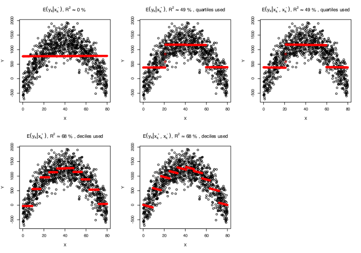
Remark 2. The use of $\boldsymbol{a}_{k}$ in the prediction approach is related to the use of piece-wise (constant) regression, where variables $\boldsymbol{x}_{k}^{*}$ are split into breaks (e.g. by quartiles or deciles) and then $\boldsymbol{a}_{k}$ are included in linear regression. Thus, we use the piece-wise method to approximate the non-linear relationship between $y$ and $\boldsymbol{x}$. Consider the following example: generate $n=1000$ observations of $X\sim\operatorname{Uniform}(0,80)$ and $Y\sim N(1300-(X-40)^{2},300)$ so we get $(y_{k},x_{k})$ pairs for $k=1,...,n$. Then, let $x_{k}$ be an auxiliary variable in the following settings: 1) $x_{k}$ is used as $x_{k}^{\circ}$ and 2) $x_{k}$ is used as $x_{k}^{*}$ where quartiles or deciles are specified, and 3) $x_{k}$ is used as $x_{k}^{*}$ and $x_{k}^{\circ}$. Figure 1 presents how the prediction changes when $x_{k}^{*}$ or $x_{k}^{\circ}$ or $x_{k}^{*}$ and $x_{k}^{\circ}$ together are included.

Figure 1: Prediction based on $x_{k}^{*}$ or $x_{k}^{\circ}$ or $x_{k}^{*}$ and $x_{k}^{\circ}$ together from the example in Remark 2. Black circles denote observed $y_{k}$, red circles denote predictions $\hat{m}_{k}$ based on the linear model

Remark 3. Mass imputation based on $\boldsymbol{x}^{*}$ or jointly on $\boldsymbol{x}^{*}$ and $\boldsymbol{x}^{\circ}$ using nearest neighbours imputation (NN) may have a larger asymptotic bias than in the case when only $\boldsymbol{x}^{\circ}$ is used since asymptomatic bias of NN estimator is of order $O_{p}(n_{B}^{-1/p})$, where $p$ is the dimension of $\boldsymbol{x}^{\circ}$, $\boldsymbol{x}^{*}$ or $\boldsymbol{x}$. Note however that $n_{B}^{-1/p}$ is only a "upper bound in probability" on bias and any random variable that is $O_{p}(n_{B}^{-1/p})$ is also $O_{p}(n_{B}^{-1/p^{\prime}})$ where $p^{\prime}>p$ and therefore this argument is only a heuristic. But nevertheless it can be treated as forming a somewhat informed hypothesis.

Remark 4. In their recent paper [78] proposed generalised additive models (GAM) for non-probability samples, where a non-linear relationship between $y$ and $\boldsymbol{x}$ is modelled through smooth functions. This, however, requires that the degree of smoothness should be specified using, for instance, cross-validation, which can be challenging [66, cf.]. In our approach one needs to decide what $\alpha$-quantiles should be specified and estimated based on probability sample $S_{B}$, which is likely to be appealing to survey practitioners.

Remark 5. A natural question that can be asked at this point is how many $\alpha$-quantiles one should consider. The question whether unique quantiles can be estimated can be answered based on probability sample $S_{B}$. For instance, it may happen that for highly skewed count variables estimated quantiles for the beginning of the distribution can be the same (e.g. $\hat{Q}_{x,0.1}=\hat{Q}_{x,0.2}$). Furthermore, if the distribution of $\boldsymbol{x}^{*}$ in a non-probability sample is significantly different from the population or probability sample it is possible that optimal $\boldsymbol{a}=\boldsymbol{0}$.

To summarise, our approach based on the inclusion of $\boldsymbol{x}_{k}^{*}$ through $\boldsymbol{a}_{k}$ in linear regression could improve predictions and provide some robustness if the imputation model is mis-specified.

4.3 Variance estimation

Variance estimation for the model-based prediction estimator $\hat{\bar{\tau}}_{y}$ involves deriving the asymptotic variance formula for $Var(\hat{\bar{\tau}}_{y}-\bar{\tau}_{y})$ under the assumed outcome regression model or the imputation model $\xi$ and the probability sampling design [75]. In our approach we do not change the assumptions regarding the outcome or the imputation model, so we can follow existing approaches to estimate variance for the prediction estimators.

For instance, consider variance of mass imputation (8) under a linear regression model proposed by [63]. It consists of two components: one refers to the probability sample given by

$$\widehat{V}_{B}=\frac{1}{N^{2}}\sum_{k\in S_{B}}\sum_{j\in S_{B}}\frac{\pi_{kj}^{B}-\pi_{k}^{B}\pi_{j}^{B}}{\pi_{kj}^{B}}d_{k}^{B}\hat{m}_{k}d_{j}^{B}\hat{m}_{j},$$ (10)

where $\pi_{kj}^{B}$ are joint inclusion probabilities, while the second one refers to the non-probability sample given by

$$\widehat{V}_{A}=\frac{1}{n_{A}^{2}}\sum_{k\in S_{A}}\hat{e}_{k}^{2}\left\{\boldsymbol{x}_{k}^{T}\left({n_{A}^{-1}\sum_{k\in S_{A}}\boldsymbol{x}_{k}\boldsymbol{x}_{k}^{T}}\right)^{-1}N^{-1}\sum_{k\in S_{B}}d_{k}^{B}\boldsymbol{x}_{k}\right\}^{2},$$ (11)

where $\hat{e}_{k}=y_{k}-\hat{m}_{k}$. If the model with $\boldsymbol{x}_{k}^{\circ}$ and $\boldsymbol{x}_{k}^{*}$ improves the model only with $\boldsymbol{x}_{k}^{\circ}$, then variance (10) will be higher since predictions $\hat{m}_{k}$ will have higher variance. On the other hand. variance (11) depends on residuals $\hat{e}_{k}^{2}$ and the sum of variables $\boldsymbol{x}_{k}$. Certainly, $\hat{e}_{k}^{2}$ will be lower as more variables are included but the second part may be larger because the sum will include $\boldsymbol{x}_{k}^{\circ}$ and $\boldsymbol{a}_{k}$. Thus, the proposed estimator may be less efficient than mass imputation proposed by [63].

5 Extension of the inverse probability weighting approach

5.1 Standard IPW estimator

[75] discussed inverse probability weighting (IPW) and its variance. Let us assume that propensity scores can be modelled parametrically as $\pi_{k}^{A}=P(R_{k}=1|\boldsymbol{x}_{k}^{\circ})=\pi(\boldsymbol{x}_{k}^{\circ},\boldsymbol{\gamma}_{0})$, where $\boldsymbol{\gamma}_{0}$ is the true value of unknown model parameters. The maximum likelihood estimator of $\pi_{k}^{A}$ is computed as $\hat{\pi}_{k}^{A}=\pi(\boldsymbol{x}_{k}^{\circ},\hat{\boldsymbol{\gamma}})$, where $\hat{\boldsymbol{\gamma}}$ maximises the log-likelihood function under full information:

$$\ell(\boldsymbol{\gamma})=\log\left\{\prod_{k=1}^{N}\left(\pi_{k}^{A}\right)^{R_{k}}\left(1-\pi_{k}^{A}\right)^{1-R_{k}}\right\}=\sum_{k\in S_{A}}\log\left(\frac{\pi_{k}^{A}}{1-\pi_{k}^{A}}\right)+\sum_{k\in U}\log\left(1-\pi_{k}^{A}\right).$$

However, in practice, reference auxiliary variables $\boldsymbol{x}$ can be supplied by the probability sample $S_{B}$, so $\ell(\boldsymbol{\gamma})$ is replaced with pseudo-likelihood (PL) function

$$\ell^{*}(\boldsymbol{\gamma})=\sum_{k\in S_{A}}\log\left(\frac{\pi_{k}^{A}}{1-\pi_{k}^{A}}\right)+\sum_{k\in S_{B}}d_{k}^{B}\log\left(1-\pi_{k}^{A}\right).$$

The maximum PL estimator $\hat{\boldsymbol{\gamma}}$ can be obtained by solving pseudo score equations by $\boldsymbol{U}(\boldsymbol{\gamma})=\partial\ell^{*}(\boldsymbol{\gamma})/\partial\boldsymbol{\gamma}=\boldsymbol{0}$. If logistic regression is assumed for $\pi_{k}^{A}$, then $\boldsymbol{U}(\boldsymbol{\gamma})$ is given by

$$\boldsymbol{U}(\boldsymbol{\gamma})=\sum_{k\in S_{A}}\boldsymbol{x}_{k}^{\circ}-\sum_{k\in S_{B}}d_{k}^{B}\pi\left(\boldsymbol{x}_{k}^{\circ},\boldsymbol{\gamma}\right)\boldsymbol{x}_{k}^{\circ}.$$ (12)

Alternatively, $\boldsymbol{U}(\boldsymbol{\gamma})=\boldsymbol{0}$ can be replaced by a system of general estimating equations [64, 75]. Let $\boldsymbol{z}(\boldsymbol{x}_{k}^{\circ},\boldsymbol{\gamma})$ be a user-specified vector of functions with the same dimensions as $\boldsymbol{\gamma}$. The general estimating equations are given by

$$\boldsymbol{G}(\boldsymbol{\gamma})=\sum_{k\in S_{A}}\boldsymbol{z}\left(\boldsymbol{x}_{k}^{\circ},\boldsymbol{\gamma}\right)-\sum_{k\in S_{B}}d_{k}^{B}\pi\left(\boldsymbol{x}_{k}^{\circ},\boldsymbol{\gamma}\right)\boldsymbol{z}\left(\boldsymbol{x}_{k}^{\circ},\boldsymbol{\gamma}\right),$$ (13)

and when we let $\boldsymbol{z}(\boldsymbol{x}_{k}^{\circ},\boldsymbol{\gamma})=\boldsymbol{x}_{k}^{\circ}/\pi(\boldsymbol{x}_{k}^{\circ},\boldsymbol{\gamma})$, then (13) reduces to calibration equations

$$\boldsymbol{G}(\boldsymbol{\gamma})=\sum_{k\in S_{A}}\frac{\boldsymbol{x}_{k}^{\circ}}{\pi\left(\boldsymbol{x}_{k}^{\circ},\boldsymbol{\gamma}\right)}-\sum_{k\in S_{B}}d_{k}^{B}\boldsymbol{x}_{k}^{\circ}.$$ (14)

In this setting unit-level data are not required to get $\sum_{k\in S_{B}}d_{k}^{B}\boldsymbol{x}_{k}^{\circ}$. Moreover, this sum can be replaced with known population totals. [64] showed that estimator (14) leads to optimal estimation when a linear regression model holds for $y$ and $\boldsymbol{x}^{\circ}$.

After estimating $\boldsymbol{\gamma}$ we obtain propensity score $\hat{\pi}_{k}^{A}$ and two versions of the IPW estimator

$$\hat{\bar{\tau}}_{\mathrm{IPW}1}=\frac{1}{N}\sum_{k\in S_{A}}\frac{y_{k}}{\hat{\pi}_{k}^{A}}\quad\text{ and }\quad\hat{\bar{\tau}}_{\mathrm{IPW}2}=\frac{1}{\hat{N}_{A}}\sum_{k\in S_{A}}\frac{y_{k}}{\hat{\pi}_{k}^{A}},$$

where $\hat{N}_{A}=\sum_{k\in S_{A}}\hat{\pi}_{k}^{A}$.

5.2 The proposed extension to the IPW estimator

The proposed modification of the IPW estimator is similar to the proposed idea of joint calibration for totals and quantiles. We modify the propensity score function $\pi_{k}^{A}$ to take into account either $\boldsymbol{x}_{k}^{*}$ through $\boldsymbol{a}_{k}$ ($\pi_{k}^{A}=\pi(\boldsymbol{x}_{k}^{*},\boldsymbol{\gamma})=\pi(\boldsymbol{a}_{k},\boldsymbol{\gamma})$) or both $\boldsymbol{x}_{k}^{\circ}$ and $\boldsymbol{x}_{k}^{*}$ ($\pi_{k}^{A}=\pi(\boldsymbol{x}_{k}^{\circ},\boldsymbol{x}_{k}^{*},\boldsymbol{\gamma})=\pi(\boldsymbol{x}_{k},\boldsymbol{\gamma})$). The proposed approach is similar to those used in the literature on survey sampling or causal inference, which offers arguments for the inclusion of higher moments for $\boldsymbol{x}^{\circ}$ auxiliary variables [62, 40, cf.]. On the other hand, it is a simpler version of the propensity score that balances distributions in comparison to methods using kernel density [61] or numerical integration [70].

In our approach we use the full or pseudo-likelihood function with the proposed modification and then solve it using (12), which takes the the following form when only $\boldsymbol{x}^{*}$ is used

$$\boldsymbol{U}(\boldsymbol{\gamma})=\sum_{k\in S_{A}}\boldsymbol{a}_{k}-\sum_{k\in S_{B}}d_{k}^{B}\pi\left(\boldsymbol{a}_{k},\boldsymbol{\gamma}\right)\boldsymbol{a}_{k},$$

or is calculated as follows if both $\boldsymbol{x}_{k}^{\circ}$ and $\boldsymbol{a}_{k}$ are used

$$\boldsymbol{U}(\boldsymbol{\gamma})=\begin{pmatrix}\sum_{k\in S_{A}}\boldsymbol{x}_{k}^{\circ}-\sum_{k\in S_{B}}d_{k}^{B}\pi\left(\boldsymbol{x}_{k}^{\circ},\boldsymbol{a}_{k},\boldsymbol{\gamma}\right)\boldsymbol{x}_{k}^{\circ}\\ \sum_{k\in S_{A}}\boldsymbol{a}_{k}-\sum_{k\in S_{B}}d_{k}^{B}\pi\left(\boldsymbol{x}_{k}^{\circ},\boldsymbol{a}_{k},\boldsymbol{\gamma}\right)\boldsymbol{a}_{k}\end{pmatrix}.$$

We can also use the generalised estimating equations in (13). In this situation $\boldsymbol{G}(\boldsymbol{\gamma})$ changes either to

$$\boldsymbol{G}(\boldsymbol{\gamma})=\sum_{k\in S_{A}}\boldsymbol{z}\left(\boldsymbol{a}_{k},\boldsymbol{\gamma}\right)-\sum_{k\in S_{B}}d_{k}^{B}\pi\left(\boldsymbol{a}_{k},\boldsymbol{\gamma}\right)\boldsymbol{z}\left(\boldsymbol{a}_{k},\boldsymbol{\gamma}\right),$$

or to

$$\boldsymbol{G}(\boldsymbol{\gamma})= \sum_{k\in S_{A}}\boldsymbol{z}\left(\boldsymbol{x}_{k}^{\circ},\boldsymbol{a}_{k},\boldsymbol{\gamma}\right)-\sum_{k\in S_{B}}d_{k}^{B}\pi\left(\boldsymbol{x}_{k}^{\circ},\boldsymbol{a}_{k},\boldsymbol{\gamma}\right)\boldsymbol{z}\left(\boldsymbol{x}_{k}^{\circ},\boldsymbol{a}_{k},\boldsymbol{\gamma}\right)$$

$$= \sum_{k\in S_{A}}\boldsymbol{z}\left(\boldsymbol{x}_{k},\boldsymbol{\gamma}\right)-\sum_{k\in S_{B}}d_{k}^{B}\pi\left(\boldsymbol{x}_{k},\boldsymbol{\gamma}\right)\boldsymbol{z}\left(\boldsymbol{x}_{k},\boldsymbol{\gamma}\right).$$

If we assume linear regression for $y$ with respect to either $\boldsymbol{a}_{k}$ or both $(\boldsymbol{x}_{k},\boldsymbol{a}_{k})$, then $\boldsymbol{G}(\boldsymbol{\gamma})$ reduces to

$$\boldsymbol{G}(\boldsymbol{\gamma})=\begin{pmatrix}\sum_{k\in S_{A}}\frac{\boldsymbol{x}_{k}^{\circ}}{\pi\left(\boldsymbol{x}_{k}^{\circ},\boldsymbol{a}_{k},\boldsymbol{\gamma}\right)}-\sum_{k\in S_{B}}d_{k}^{B}\boldsymbol{x}_{k}^{\circ}\\ \sum_{k\in S_{A}}\frac{\boldsymbol{a}_{k}}{\pi\left(\boldsymbol{x}_{k}^{\circ},\boldsymbol{a}_{k},\boldsymbol{\gamma}\right)}-\sum_{k\in S_{B}}d_{k}^{B}\boldsymbol{a}_{k}\end{pmatrix}=\sum_{k\in S_{A}}\frac{\boldsymbol{x}_{k}}{\pi\left(\boldsymbol{x}_{k},\boldsymbol{\gamma}\right)}-\sum_{k\in S_{B}}d_{k}^{B}\boldsymbol{x}_{k}.$$ (15)

This simple modification has important implications for inference based on the IPW estimator:

• estimated propensity scores will reproduce either known or estimated moments as well as specified $\alpha$-quantiles (e.g. median, quartiles or deciles). We use more information regarding count or continuous variables if they are available in both datasets;

• inclusion of $\alpha$-quantiles in the $\pi_{k}^{A}$ approximate relationship between inclusion $R$ and $\boldsymbol{x}^{*}$, as discussed in section 4. Thus, the inclusion of $\alpha$-quantiles makes estimates more robust to model mis-specification for the propensity and outcome model when calibrated IPW is used.

Inference based on the IPW estimator does not change as we add new variables to the propensity score model. We do not assume that quantiles are based on, say, instrumental variables or are collected through paradata [67] but treat them as if we were adding higher moments.

5.3 Variance estimation

As in the case of the MI estimator, we can use the already developed approach to estimating variance for the IPW estimator. Following the same regularity conditions as in [49], we just modify the equation $\boldsymbol{\Phi}_{n}(\boldsymbol{\eta})=\boldsymbol{0}$ [75] by imposing constraints on quantiles, and in the case of $\boldsymbol{z}(\boldsymbol{x}_{k},\boldsymbol{\gamma})=\frac{\boldsymbol{x}_{k}}{\pi_{k}(\boldsymbol{x}_{k},\boldsymbol{\gamma})}$, the equation will be given as

$$\boldsymbol{\Phi}_{n}(\boldsymbol{\eta})=N^{-1}\begin{pmatrix}\sum_{k\in U}R_{k}\frac{y_{i}-\mu}{\pi(\boldsymbol{x}_{k}^{\circ},\boldsymbol{a}_{k},\boldsymbol{\gamma})}\\ \sum_{k\in U}R_{k}\frac{\boldsymbol{x}^{\circ}_{k}}{\pi(\boldsymbol{x}_{k}^{\circ},\boldsymbol{a}_{k},\boldsymbol{\gamma})}-\sum_{k\in S_{B}}d_{k}^{B}\boldsymbol{x}_{k}^{\circ}\\ \sum_{k\in U}R_{k}\frac{\boldsymbol{a}_{k}}{\pi(\boldsymbol{x}_{k}^{\circ},\boldsymbol{a}_{k},\boldsymbol{\gamma})}-\sum_{k\in S_{B}}d_{k}^{B}\boldsymbol{a}_{k}\end{pmatrix}.$$ (16)

[49] provided the analytical form of the variance estimator when logistic regression is used for $\pi_{k}$. Our approach, based on $\boldsymbol{a}_{k}$ or $\boldsymbol{x}_{k}$, will lead to higher variance as the number of variables can be significantly larger than $\boldsymbol{x}_{k}^{\circ}$.

6 Extension to doubly robust estimators

6.1 Doubly robust estimators

Finally, we can combine the prediction and inverse probability weighting approach using a doubly robust (DR) estimator of the population $\bar{\tau}_{y}$. The DR estimator with propensity scores $\pi_{k}^{A}$ and mean responses $m_{k}=E_{\xi}(y_{k}|\boldsymbol{x}_{k}^{\circ})$ has the following general form

$$\tilde{\bar{\tau}}_{DR}=\frac{1}{N}\sum_{k\in S_{A}}\frac{y_{k}-m_{k}}{\pi_{k}^{A}}+\frac{1}{N}\sum_{k\in U}m_{k}.$$ (17)

If the $\hat{\pi}_{k}^{A}$ and $\hat{m}_{k}$ are estimated on the basis on two samples ($S_{A}$ and $S_{B}$), then the DR estimator is given by

$$\hat{\bar{\tau}}_{DR1}=\frac{1}{N}\sum_{k\in S_{A}}\frac{y_{k}-\hat{m}_{k}}{\hat{\pi}_{k}^{A}}+\frac{1}{N}\sum_{k\in S_{B}}d_{k}^{B}\hat{m}_{k},$$ (18)

or

$$\hat{\bar{\tau}}_{DR2}=\frac{1}{\hat{N}_{A}}\sum_{k\in S_{A}}\frac{y_{k}-\hat{m}_{k}}{\hat{\pi}_{k}^{A}}+\frac{1}{\hat{N}_{B}}\sum_{k\in S_{B}}d_{k}^{B}\hat{m}_{k},$$ (19)

where $\hat{N}_{A}=\sum_{k\in S_{A}}(\pi_{k}^{A})^{-1}$ and $\hat{N}_{B}=\sum_{k\in S_{B}}d_{k}^{B}$.

6.2 The proposed extension to the doubly robust estimator

Again, in our approach we modify estimators (17)-(19) to take into account $\boldsymbol{x}_{k}^{*}$ through $\boldsymbol{a}_{k}$. For example, estimator (19) with only $\boldsymbol{x}_{k}^{*}$ is given by

$$\hat{\bar{\tau}}_{DR2}=\frac{1}{\hat{N}_{A}}\sum_{k\in S_{A}}d_{k}^{A}\left\{y_{k}-m\left(\boldsymbol{a}_{k},\hat{\boldsymbol{\gamma}}\right)\right\}+\frac{1}{\hat{N}_{B}}\sum_{k\in S_{B}}d_{k}^{B}m\left(\boldsymbol{a}_{k},\hat{\boldsymbol{\beta}}\right),$$ (20)

where $d_{k}^{A}=\pi\left(\boldsymbol{a}_{k},\hat{\boldsymbol{\gamma}}\right)^{-1}$, $\hat{N}_{A}=\sum_{k\in S_{A}}d_{k}^{A}$ and $\hat{N}_{B}=\sum_{k\in S_{B}}d_{k}^{B}$ and if both $\boldsymbol{x}_{k}^{\circ}$ and $\boldsymbol{a}_{k}$ are used

$$\hat{\bar{\tau}}_{DR2}=\frac{1}{\hat{N}_{A}}\sum_{k\in S_{A}}d_{k}^{A}\left\{y_{k}-m\left(\boldsymbol{x}_{k}^{\circ},\boldsymbol{a}_{k},\hat{\boldsymbol{\gamma}}\right)\right\}+\frac{1}{\hat{N}_{B}}\sum_{k\in S_{B}}d_{k}^{B}m\left(\boldsymbol{x}_{k}^{\circ},\boldsymbol{a}_{k},\hat{\boldsymbol{\beta}}\right),$$ (21)

where $d_{k}^{A}=\pi\left(\boldsymbol{x}_{k}^{\circ},\boldsymbol{a}_{k},\hat{\boldsymbol{\gamma}}\right)^{-1}$.

If we include $\boldsymbol{a}_{k}$ in both models, then the resulting DR estimator can become more robust to model mis-specifications because the non-linear relationship in the selection and outcome model is approximated with linear models and quantiles.

[75] offers a discussion on how to estimate parameters $(\boldsymbol{\beta},\boldsymbol{\gamma})$. One can consider the way of estimating $(\boldsymbol{\beta},\boldsymbol{\gamma})$ proposed by [77], which includes a specific way of selecting variables.

6.3 Variance estimation

As in the previous cases, we can use the approach already proposed in the literature. In particular, if we are interested in estimating the variance of (21), one can consider the bootstrap approach, as suggested by [76]. In the simulation study we used the variance estimator of (18), as proposed by [49] for (20) assuming that the population size is known.

7 Simulation study

Our simulation study to compare the proposed estimators follows the procedure described in [65] and [78]. We generate a finite population $\mathcal{F}_{N}=\{\boldsymbol{X}_{k}=(X_{k1},X_{k2}),\boldsymbol{Y}_{k}=(Y_{k1},Y_{k2}):k=1,\ldots,N\}$ with size $N=20,000$, where $Y_{k1}$ is the continuous outcome, $Y_{k2}$ is the binary outcome, $X_{k1}\sim N(1,1)$ and $X_{k2}\sim\operatorname{Exp}(1)$. From this population, we select a big sample $S_{A}$ of size approximately $14,000$ (for PM1) and $10,000$ (for PM2), depending on the selection mechanism, assuming the inclusion indicator $\delta_{Bk}\sim\text{Bernoulli}(p_{k})$ with $p_{k}$ denoting the inclusion probability for unit $k$. Then we select a simple random sample $S_{B}$ of size $n=1,000$ from $\mathcal{F}_{N}$. The goal is to estimate the population mean $N^{-1}\sum_{k=1}^{N}Y_{kj}$, $j=1,2$.

The finite population $\mathcal{F}_{N}$ and the big sample $S_{A}$ were generated using the outcome variables (denoted as outcome model; OM) and the inclusion probability (denoted as probability model; PM) presented in Table 7.1, where $\alpha_{k}\sim N(0,1)$ and $\epsilon_{k}\sim N(0,1)$ and $X_{k1},X_{k2},\alpha_{k}$ and $\epsilon_{k}$ are mutually independent. The variable $\alpha_{k}$ induces dependence of $Y_{k1}$ and $Y_{k2}$ even after adjusting for $X_{k1}$ and $X_{k2}$.

Table 7.1: Outcome models and the probability of inclusion in sample $SA$ used in the simulation study

Type	Form	Formulae
Continuous	linear (OM1)	$Y_{k1}=1+X_{k1}+X_{k2}+\alpha_{k}+\epsilon_{k}$
	non-linear (OM2)	$Y_{k2}=0.5(X_{k1}-1.5)^{2}+X_{k2}^{2}+\alpha_{k}+\epsilon_{k}$
Binary	linear (OM3)	$P(Y_{k1}=1|X_{k1},X_{k2};\alpha_{k})=\operatorname{logit}(1+X_{k1}+X_{k2}+\alpha_{k})$
	non-linear (OM4)	$P(Y_{k2}=1|X_{k1},X_{k2};\alpha_{k})=\operatorname{logit}\left\{0.5(X_{k1}-1.5)^{2}+X_{k2}^{2}+\alpha_{k}\right\}$
Selection ($S_{A}$)	linear (PM1)	$\operatorname{logit}(p_{k})=X_{k2}$
	non-linear (PM2)	$\operatorname{logit}(p_{k})=-3+(X_{k1}-1.5)^{2}+(X_{k2}-2)^{2}$

In the results, we report Monte Carlo bias (B), standard error (SE) and relative mean square error (RMSE) based on $R=500$ simulations for each $Y$ variables: $\text{B}=\bar{\hat{\tau}}-\hat{\tau}$, $\text{SE}=\sqrt{\frac{\sum_{r=1}^{R}\left(\hat{\tau}^{(r)}-\bar{\hat{\tau}}\right)^{2}}{R-1}}$ and $\text{RMSE}=\sqrt{\text{B}^{2}+\text{SE}^{2}}$, where $\bar{\hat{\tau}}=\sum_{r=1}^{R}\hat{\tau}^{(r)}/R$ and $\hat{\tau}^{\left(r\right)}$ is an estimate of the mean in the $r$-th replication. The simulation was conducted in R [68] using the nonprobsvy [51] and the jointCalib [43] packages. To solve calibration constraints in the IPW estimator we used Newton’s method with a trust region [54, cf.] implemented in the nleqslv [60] package.

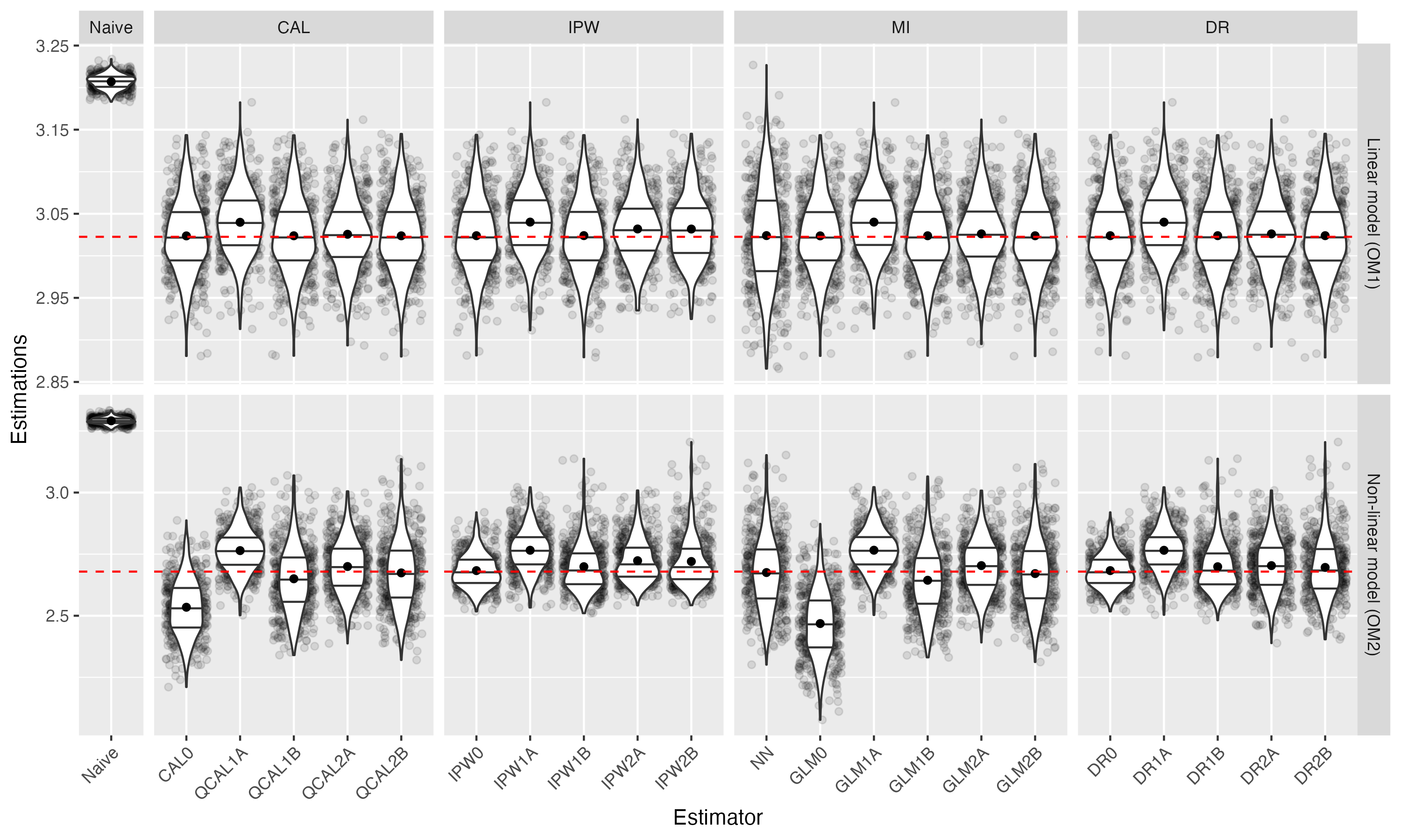
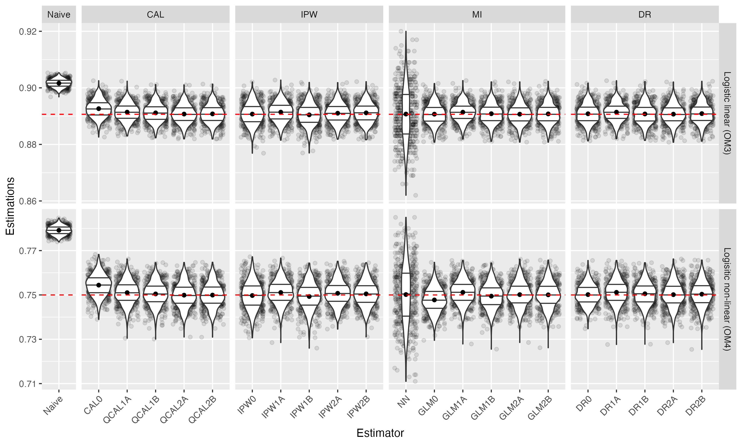
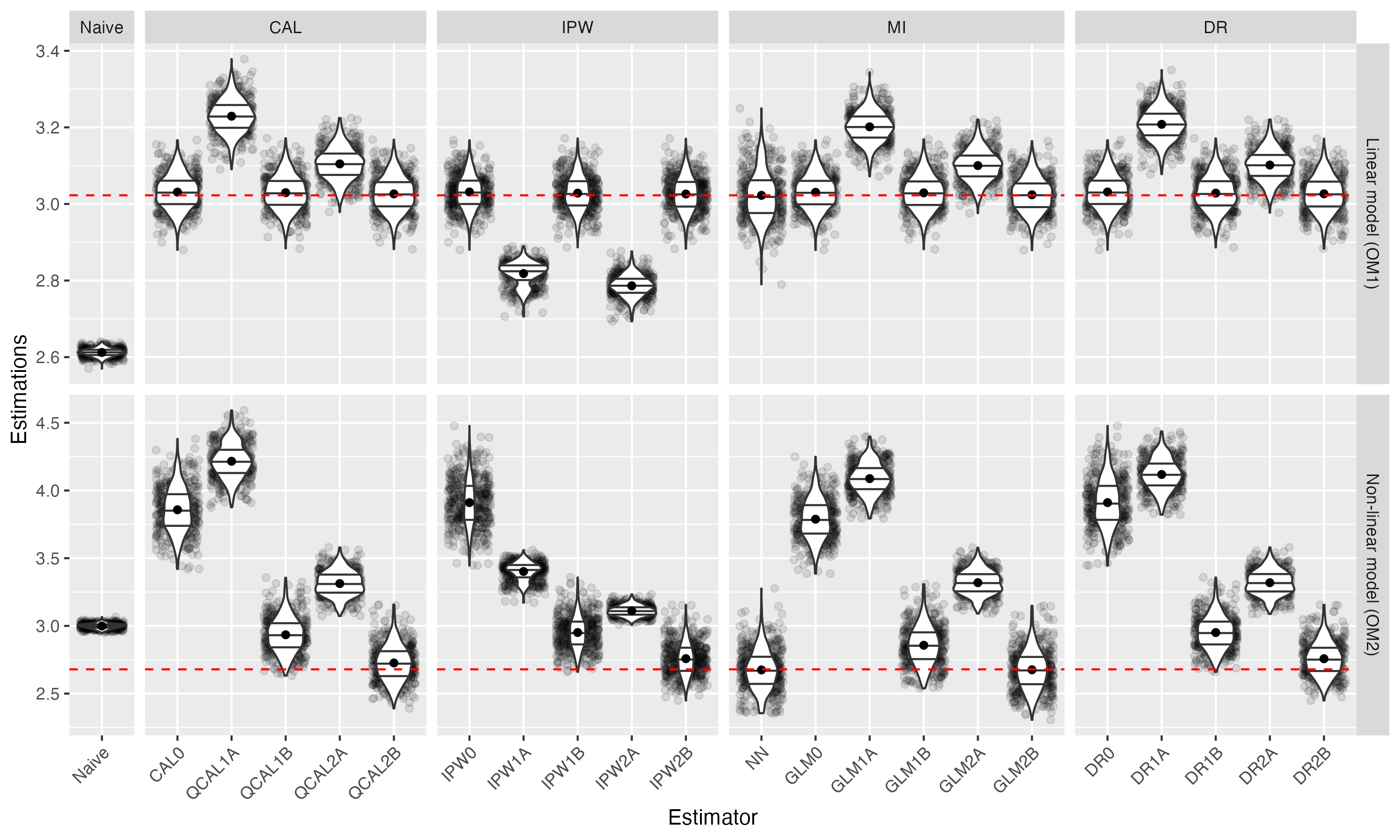
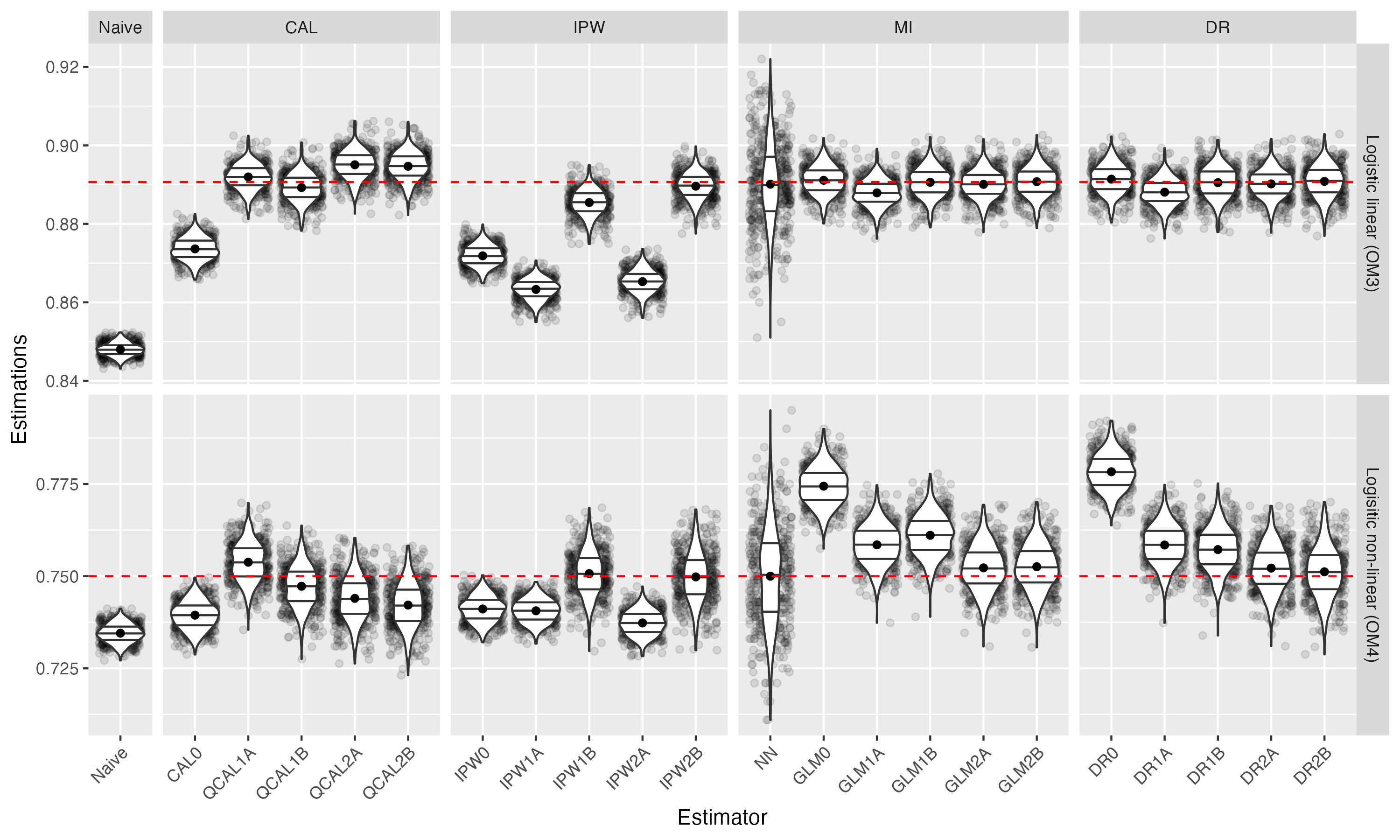
Simulation results are presented in Tables 7.2 and 7.3, while their graphical representations are included in the Appendix in Figures 4–7. Table A.1 in the Appendix shows the empirical coverage (CR) of confidence intervals based on analytic variance estimators for MI, IPW and DR estimators.

The following estimators were considered with a set of calibration equations including totals or quantiles for auxiliary variables estimated from sample $S_{B}$:

• Naïve calculated from sample $S_{A}$ only,

• CAL using estimated totals for auxiliary variables $x_{1},x_{2}$ only (CAL0), estimated quartiles for auxiliary variables $x_{1},x_{2}$ only (CAL1A), CAL0 with estimated quartiles (CAL1B), estimated deciles for auxiliary variables $x_{1},x_{2}$ only (CAL2A), CAL0 with estimated deciles (CAL2B) – calibration was conducted using raking to avoid negative weights,

• MI NN with 5 neighbours using $x_{1},x_{2}$ only (NN),

• MI GLM using $x_{1},x_{2}$ as $\boldsymbol{x}^{\circ}$ only (GLM0), GLM1A: $x_{1},x_{2}$ as $\boldsymbol{x}^{*}$ with quartiles estimated from $S_{B}$, GLM1B combines GLM0 with GLM1A, GLM2A: $x_{1},x_{2}$ as $\boldsymbol{x}^{*}$ with estimated deciles for $x_{1},x_{2}$, GLM2B combines GLM0 with GLM2A – for OM1 we use linear and for OM2 logistic regression,

• calibrated IPW (given by (15)) using : estimated totals for $x_{1},x_{2}$ only (IPW0), estimated quartiles for $x_{1},x_{2}$ (IPW1A), IPW1B combines IPW0 with IPW1A, estimated deciles for $x_{1},x_{2}$ only (IPW2A), IPW2B combines IPW0 with IPW2A,

• DR: DR0 combines IPW0 with GLM0, DR1A combines IPW1A with GLM1A, DR1B combines IPW1B with GLM1B, DR2A combines IPW2A with GLM2B and DR2B combines IPW2B with GLM2B – linear regression was applied for OM1, while logistic regression – for OM2.

Table 7.2 contains results for continuous outcome variables i.e. OM1 and OM2 with propensity score model PM1 and PM2. In Scenario I, the proposed approach to MI is similar to standard regression using $x_{1}$ and $x_{2}$ only. Even if the model contains only quantiles (quartiles or deciles), its RMSE is comparable to that of the standard model (GLM0). MI GLM estimators are more efficient than MI NN and the empirical coverage rate (CR) is around 95% with the expection for GLM1A that contains only quartiles. In the case of IPW in Scenario I estimators yield similar values of RMSE, which increase as the number of variables used for calibration increases. DR estimators are unbiased and have similar RMSE and CR close to 95%.

In Scenario II, with non-linear selection, estimators with only quartiles (1A) or deciles (2B) are characterised by large bias. The empirical CR is significantly lower and close to 0. However, the inclusion of both $\boldsymbol{x}^{\circ}$ and $\boldsymbol{x}^{*}$ makes these estimators asymptotically unbiased. As expected, estimators IPW1B and IPW2B have a higher variance due to a larger number of variables in the calibration equations.

In Scenario III the PM model is non-linear and thus the inclusion of quantiles for the MI GLM approximates this relation. Bias of the GLM0 estimator is significantly larger and the resulting empirical CR for the proposed approach is close to 95%. The empirical CRs for all proposed mass imputation and doubly robust estimators are close to the nominal level, while they vary for IPW estimators, particularly for those with quartiles and deciles only.

Table 7.2: Results for continuous Y (OM1 and OM2; B, SE and RMSE are multiplied by 100)

	Scenario I			Scenario II			Scenario III			Scenario IV
OM	linear (1)			linear (1)			non-linear (2)			non-linear (2)
PM	linear (1)			non-linear (2)			linear (1)			non-linear (2)
	B	SE	RMSE	B	SE	RMSE	B	SE	RMSE	B	SE	RMSE
Naïve	18.44	0.80	18.50	-41.04	1.00	41.10	61.21	1.40	61.20	31.96	1.80	32.00
Calibration estimators
CAL0	0.11	4.40	4.40	0.84	4.40	4.50	-14.47	11.30	18.40	117.82	16.40	119.00
QCAL1A	1.73	3.90	4.30	20.65	4.30	21.10	8.53	8.40	12.00	153.64	12.50	154.20
QCAL1B	0.12	4.40	4.40	0.69	4.50	4.60	-2.91	13.20	13.50	25.52	12.90	28.60
QCAL2A	0.30	4.10	4.20	8.20	4.10	9.20	2.06	10.70	10.90	63.35	9.20	64.00
QCAL2B	0.12	4.40	4.40	0.37	4.50	4.50	-0.53	13.80	13.80	4.70	13.30	14.10
Mass imputation
NN	0.15	6.00	6.00	-0.01	6.40	6.40	-0.38	14.50	14.50	-0.46	14.80	14.80
GLM0	0.11	4.40	4.40	0.79	4.40	4.50	-21.09	13.40	25.00	110.86	14.80	111.80
GLM1A	1.75	3.90	4.30	17.88	4.00	18.30	8.68	8.50	12.10	140.84	11.30	141.30
GLM1B	0.13	4.40	4.40	0.64	4.50	4.50	-3.51	13.50	14.00	17.79	14.30	22.80
GLM2A	0.35	4.10	4.20	7.76	4.00	8.70	2.43	10.70	11.00	64.00	8.80	64.60
GLM2B	0.13	4.40	4.40	0.13	4.50	4.50	-0.80	13.90	13.90	-0.32	14.60	14.60
Inverse probability weighting
IPW0	0.13	4.40	4.40	0.86	4.40	4.50	0.40	6.80	6.90	123.12	17.60	124.40
IPW1A	1.75	3.90	4.30	-20.44	3.10	20.70	8.67	8.40	12.10	72.22	6.70	72.50
IPW1B	0.14	4.40	4.40	0.57	4.50	4.60	1.99	9.80	10.00	27.19	12.20	29.80
IPW2A	0.93	3.80	3.90	-23.64	2.80	23.80	4.42	8.50	9.60	43.22	3.80	43.40
IPW2B	0.92	3.90	4.00	0.33	4.60	4.60	4.11	10.20	11.00	7.89	12.30	14.60
Doubly robust
DR0	0.13	4.40	4.40	0.86	4.40	4.50	0.40	6.80	6.90	123.12	17.60	124.40
DR1A	1.74	3.90	4.30	18.54	4.10	19.00	8.65	8.50	12.10	143.88	11.60	144.40
DR1B	0.14	4.40	4.40	0.57	4.50	4.60	1.98	9.80	10.00	27.19	12.20	29.80
DR2A	0.35	4.20	4.20	7.90	4.00	8.90	2.43	10.70	11.00	64.00	8.90	64.60
DR2B	0.14	4.40	4.40	0.39	4.60	4.60	1.69	12.40	12.60	7.82	12.30	14.60

Finally, Scenario IV includes two non-linear models. In this situation none of the standard estimators is correct as both PM and OM are mis-specified. The proposed approach, which includes either $\boldsymbol{x}^{*}$ or $\boldsymbol{x}$, leads to a significant decrease in bias, particularly for estimators with 2B combination of variables. RMSE values for MI GLM2B, IPW2B and DR2B are comparable with those obtained for the MI NN estimator and their empirical coverage rate is close to 95%.

Table 7.3 contains results for binary outcome variables, i.e. OM1 and OM2, with propensity score model PM1 and PM2. For all scenarios the proposed approaches produce nearly unbiased estimators, which suggests that for the binary case it makes no significant difference whether $\boldsymbol{x}^{*}$ only or $\boldsymbol{x}^{\circ}$ and $\boldsymbol{x}^{*}$ are included. The empirical CR is close to 95% with some exceptions for Scenario IV. RMSE values for the proposed estimators are comparable or smaller than those for MI NN, with the biggest difference for DR estimators.

Table 7.3: Results for binary Y (OM3 and OM4; Bias, SE and RMSE are multiplied by 100)

	Scenario I			Scenario II			Scenario III			Scenario IV
OM	linear (3)			linear (3)			non-linear (4)			non-linear (4)
PM	linear (1)			non-linear (2)			linear (1)			non-linear (2)
	B	SE	RMSE	B	SE	RMSE	B	SE	RMSE	B	SE	RMSE
Naïve	1.10	0.14	1.11	-4.27	0.17	4.27	2.92	0.20	2.92	-1.55	0.25	1.57
Calibration estimators
CAL0	0.20	0.31	0.37	-1.70	0.29	1.73	0.44	0.49	0.66	-1.06	0.38	1.12
QCAL1A	0.08	0.31	0.32	0.13	0.32	0.35	0.10	0.52	0.53	0.38	0.53	0.65
QCAL1B	0.05	0.32	0.32	-0.14	0.36	0.39	0.05	0.53	0.53	-0.27	0.56	0.63
QCAL2A	0.01	0.32	0.32	0.44	0.36	0.57	-0.01	0.54	0.54	-0.60	0.60	0.85
QCAL2B	0.01	0.33	0.33	0.40	0.36	0.54	-0.01	0.54	0.54	-0.78	0.61	1.00
Mass imputation
NN	0.01	0.97	0.97	-0.05	1.07	1.07	0.02	1.35	1.35	-0.00	1.32	1.32
GLM0	0.00	0.35	0.35	0.04	0.36	0.37	-0.23	0.55	0.59	2.44	0.51	2.49
GLM1A	0.07	0.33	0.34	-0.28	0.34	0.43	0.12	0.54	0.55	0.85	0.54	1.01
GLM1B	0.02	0.35	0.35	-0.01	0.37	0.37	-0.05	0.56	0.56	1.11	0.56	1.24
GLM2A	0.00	0.34	0.34	-0.06	0.35	0.36	0.01	0.56	0.56	0.23	0.61	0.65
GLM2B	0.01	0.35	0.35	0.01	0.37	0.37	0.00	0.57	0.57	0.26	0.62	0.67
Inverse probability weighting
IPW0	0.01	0.39	0.39	-1.88	0.27	1.90	-0.03	0.62	0.62	-0.89	0.35	0.96
IPW1A	0.08	0.34	0.35	-2.74	0.27	2.75	0.11	0.54	0.55	-0.94	0.31	0.99
IPW1B	-0.02	0.39	0.39	-0.52	0.34	0.62	-0.07	0.61	0.61	0.07	0.61	0.61
IPW2A	0.04	0.34	0.35	-2.54	0.30	2.55	0.07	0.53	0.54	-1.27	0.33	1.31
IPW2B	0.05	0.35	0.35	-0.10	0.34	0.36	0.05	0.55	0.55	-0.02	0.69	0.69
Doubly robust
DR0	0.02	0.35	0.35	0.07	0.37	0.37	0.02	0.47	0.47	2.83	0.49	2.87
DR1A	0.08	0.33	0.34	-0.26	0.34	0.42	0.12	0.54	0.55	0.85	0.54	1.00
DR1B	0.01	0.35	0.35	-0.01	0.40	0.40	0.05	0.52	0.52	0.72	0.58	0.93
DR2A	0.00	0.34	0.34	-0.05	0.36	0.36	0.01	0.56	0.56	0.22	0.62	0.66
DR2B	0.02	0.35	0.35	0.02	0.41	0.41	0.03	0.57	0.58	0.12	0.69	0.70

The simulation study suggests that the inclusion of quantiles in the MI, IPW and DR estimators leads to better estimates, particularly when both models are mis-specified. Assuming that continuous or count variables are available in both sources, one should therefore consider using quantiles to make results more robust.

8 Real data application

8.1 Data description

In this section we present an attempt to integrate administrative and survey data about job vacancies for the end of 2022Q2 in Poland. The aim was to estimate the share of vacancies aimed at Ukrainian workers. After the Russian invasion of Ukraine on 24 February 2022, around 3.5 million persons (mainly women and children) arrived in Poland between 24 February and mid-May 2022 [56]. Some of them went to other European countries, but about 1 million stayed in Poland (as of 2023, cf. [73]).

The first source we used is the Job Vacancy Survey (JVS, known in Poland as the Labour Demand Survey), which is a stratified sample of 100,000 units, with a response rate of about 60% ($S_{B}$). The survey population consists of companies and their local units with 1 or more employees. The sampling frame includes information about NACE (19 levels), region (16 levels), sector (2 levels), size (3 levels) and the number of employees according to administrative data integrated by Statistics Poland (RE). The JVS sample contains 304 strata created separately for enterprises with up to 9 employees and those with more than 10 employees [72, cf.]

The survey measures whether an enterprise has a job vacancy at the end of the quarter (on June 31, 2022) according to the following definition: vacancies are positions or jobs that are unoccupied as a result of employee turnover or newly created positions or jobs that simultaneously meet the following three conditions: (1) the jobs were actually vacant on the day of the survey, (2) the employer made efforts to find people willing to take on the job, (3) if suitable candidates were found to fill the vacancies, the employer would be willing to hire them. In addition, the JVS restricts the definition of vacancies by excluding traineeships, mandate contracts, contracts for specific work and B2B contracts. Of the 60,000 responding units, around 7,000 reported at least one vacancy. Our target population included units with at least one vacancy, which according to the survey was between 38,000 and 43,000 at the end of 2022Q2.

The second source is the Central Job Offers Database (CBOP), which is a register of all vacancies submitted to Public Employment Offices (PEOs – $S_{A}$). CBOP is available online and can be accessed via API. CBOP includes all types of contracts and jobs outside Poland, so data cleaning was carried out to align the definition of a vacancy with that used in the JVS. CBOP data collected via API include information about whether a vacancy is outdated (e.g. 17% of vacancies were outdated when downloaded at the end of 2022Q2). CBOP also contains information about unit identifiers (REGON and NIP), so we were able to link units to the sampling frame to obtain auxiliary variables with the same definitions as in the survey (24% of records did not contain an identifier because the employer can withhold this information). The final CBOP dataset contained about 8,500 units included in the sampling frame.

The overlap between JVS and CBOP was around 2,600 entities (around 4% of the JVS sample and 30% of CBOP), but only 30% of these reported at least one vacancy in the JVS survey. This suggests significant under-reporting in the JVS, which, however, is a problem beyond the scope of this paper. For the empirical study we treated both sources as separate and their correct treatment with the proposed methods will be investigated in the future.

8.2 Analysis and results

We defined our target variable as follows: $Y$ is the share of vacancies that have been translated into Ukrainian (denoted as UKR), calculated separately for each unit. After the Russian aggression, many online job advertising services introduced information on whether the employer is particularly interested in employing Ukrainians (e.g. the Ukrainian version of the website was available, and job ads featured the following annotation: "We invite people from Ukraine").

Table 8.1: Quantiles of registered employment (RE) for JVS, CBOP and the target variable UKR at the end of 2022Q2

Decile of the RE	JVS	CBOP	CBOP-UKR
10%	3	4	4
20%	4	6	5
30%	5	8	8
40%	6	13	11
50%	8	20	18
60%	10	32	28
70%	17	51	48
80%	37	90	91
90%	100	211	215

Table 8.1 shows the distribution of registered employment according to the JVS survey, companies observed in the CBOP and companies willing to employ Ukrainians (with at least one vacancy translated into Ukrainian; denoted as CBOP-UKR). Companies observed in the CBOP are on average larger than those responding to the JVS. The median employment for JVS was 6, while for CBOP and CBOP-UKR – 20 and 18 employees, respectively. This suggests that companies are selected into the CBOP depending on their size.

Figure 2: The distribution of 4 auxiliary variables in the sources at the end of 2022Q2. JVS: the total sample, JVS (vacancies): companies with at least one vacancy, CBOP: register data set, CBOP-UKR: units with at least one vacancy translated into Ukrainian

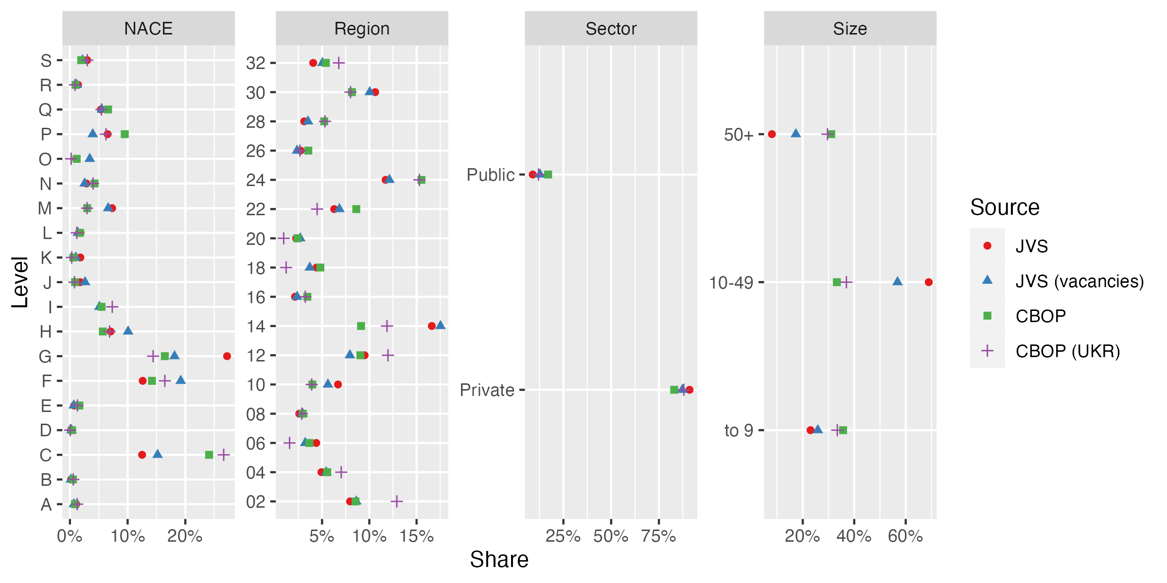
The distributions of four categorical variables in the two sources are shown in Figure 2. The largest discrepancies between the sources can be seen in the case of company size, where the shares in CBOP are almost equal. There are some differences for selected regions (e.g. 14 Mazowieckie with Warsaw, the capital of Poland; 02 Dolnośląskie with Wrocław and 12 Małopolskie with Kraków). Regions from the eastern part of Poland (06 Lubelskie, 18 Podkarpackie, 20 Podlaskie), but also Pomorskie (22) with Tricity are characterised by the lowest share of vacancies for Ukrainians. The largest differences in terms of NACE are found for manufacturing (C), wholesale and retail trade (G) and hotels and restaurants (I).

Figure 3: The target variable (the share of ads directed at Ukrainians) depending on 5 auxiliary variables at the end of 2022Q2

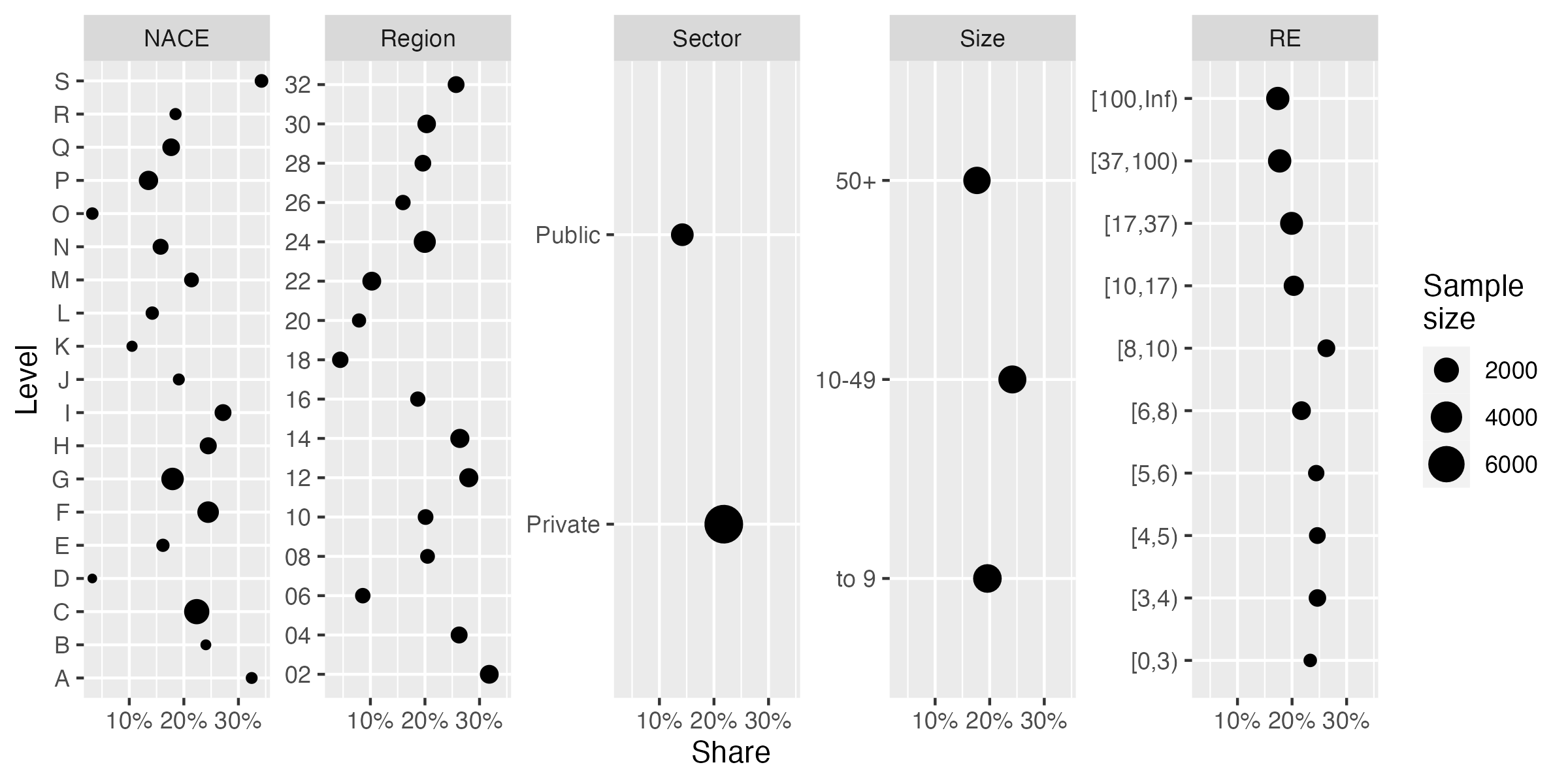
Figure 3 shows the share of vacancies targeted at Ukrainians according to four categorical variables and deciles of registered employment (RE) based on deciles estimated from the JVS survey. In general, the shares range between about 10% and 30%, especially across regions. The shares for the RE deciles range between 17% for the largest units and 26% for the median RE (8 employees).

The following combinations of variables were considered:

• Set 0: Region (16 levels), NACE (19 levels), Sector (2 levels), Size (3 levels), $\log$(RE), $\log$(# vacancies) (the number of vacancies), $I$(# vacancies = 1) (whether employer seeks only one person),

• Set 1A: Set 0 (without $\log$(RE)) + Quartiles of the RE (estimated from the JVS),

• Set 2A: Set 0 + Quartiles of the RE,

• Set 1B: Set 0 (without $\log$(RE)) + Deciles of the RE (without 10%),

• Set 2B: Set 0 + Deciles of RE (without 10%).

We decided not to include the number of vacancies as the $\boldsymbol{x}^{*}$ variable, as almost 45% of vacancies were equal to 1 for CBOP and almost 30% for JVS. We consider the following estimators, assuming linear regression (for the NN estimator we used $\log$(RE) and $\log$(# vacancies) only):

• Calibration estimators: CAL, QCAL1A, QCAL1B, QCAL2A, QCAL2B,

• MI: GLM0, GLM1A, GLM1A, GLM2A, GLM2B, NN,

• IPW: IPW0, IPW1A, IPW1B, IPW2A, IPW2B,

• DR: DR0, DR1A, DR1B, DR2A, DR2B.

Variance was estimated using the following bootstrap approach: 1) JVS sample was resampled using a stratified bootstrap approach, 2) CBOP was resampled using simple random sampling with replacement. This procedure was repeated $B=500$ times. Table 8.2 shows point estimates (denoted as Point), bootstrap standard errors (denoted as SE), the coefficients of variation (CV) and 95% confidence intervals.

Table 8.2: Estimates of the share of job vacancies aimed at Ukrainians at the end of 2022Q2 in Poland

Estimator	Point	SE	CV	2.5%	97.5%
Naïve
Naïve	20.51	–	–	–	–
Calibration
CAL	21.98	0.62	2.83	20.76	23.20
QCAL1A	21.80	0.63	2.88	20.57	23.03
QCAL1B	21.99	0.64	2.89	20.74	23.23
QCAL2A	22.04	0.74	3.37	20.59	23.50
QCAL2B	22.20	0.76	3.44	20.70	23.69
Mass imputation
GLM0	22.68	0.60	2.66	21.50	23.87
GLM1A	22.35	0.59	2.66	21.18	23.51
GLM1B	22.56	0.60	2.68	21.38	23.74
GLM2A	22.61	0.61	2.71	21.41	23.81
GLM2B	22.72	0.62	2.71	21.51	23.93
NN	25.88	6.28	24.26	13.58	38.19
Inverse probability weighting
IPW0	21.75	0.64	2.92	20.50	23.00
IPW1A	21.53	0.63	2.92	20.30	22.76
IPW1B	21.69	0.63	2.92	20.45	22.93
IPW2A	21.69	0.65	2.99	20.42	22.96
IPW2B	21.74	0.65	2.98	20.47	23.00
Doubly robust
DR0	21.75	0.64	2.92	20.50	23.00
DR1A	21.53	0.63	2.92	20.30	22.76
DR1B	21.69	0.63	2.92	20.45	22.93
DR2A	21.69	0.65	2.99	20.42	22.96
DR2B	21.74	0.65	2.98	20.47	23.00

When analysing the results presented in Table 8.2, one see that the point estimates produced by all the estimators in the study are at a similar level and fluctuate around 22%, with the exception of the Naïve estimators, for which the estimated share of job vacancies aimed at Ukrainians is lower and amounts to 20.51%, and the NN estimator for which the percentage was close to 26%. Taking into account the precision of the estimates (CV), it is relatively low only for the NN estimator. This may be due to the fact that the variables used in the NN method to find neighbours were, in many cases, extremely right-skewed. CV values for the other estimators are similar, with the exception of the GLM estimators, for which the measure of precision is the lowest of all estimators considered in the study.

9 Summary

Recent years have seen a revolution in survey research with regard to the use and integration of new data sources for statistical inference. Efforts in this area have focused on the integration of survey data and inference based on non-probability samples, with applications in official statistics [69]. This is mainly because probability samples tend to be very costly and are associated with respondent burden. On the other hand, statistical inference based on non-probabilities samples is a real challenge, mainly owing to bias inherent in the estimation process. Consequently, it is necessary to develop new methods of statistical inference based on non-probability samples, which could be be useful in real applications [75].

In this paper we have described a joint approach to calibration for non-probability surveys which is based on the idea of calibration proposed by [55] for totals and by [59] for quantiles. We use the joint approach to extend existing inference methods for non-probability samples, including inverse probability weighting, mass imputation and doubly robust estimators. Thanks to our approach, for some of the methods considered in the article (IPW and DR) it is possible to reproduce not only totals for a set of auxiliary variables but also for a set of quantiles (or estimated quantiles). Such a solution improves robustness against model mis-specification, helps to decrease bias and improves the efficiency of estimation. These gains have been confirmed by our simulation study, in which we have shown that the inclusion of quantiles for mass imputation, inverse probability weighting and doubly robust estimators improves the quality of estimates.

The estimators proposed in this paper, based on the classical idea of calibration for totals and quantiles, can have real-life applications, provided continuous variables of sufficient quality are available to be used as auxiliary variables. The example of our empirical study, in which we estimated the share of vacancies aimed at Ukrainian workers, shows that the proposed methods produce estimates of high precision.

As regards aspects not addressed in this paper, one issue worth investigating further is the problem of under-coverage in non-probability samples, which is related to the violation of the positivity assumption (A2). The approach proposed in the paper equates the distributions of variables between the probability (or the population) and the non-probability sample and can serve as an alternative to other approaches proposed in the literature, which consist in, for example, using an additional sample of individuals from the population not covered by the non-probability sample [50, cf.].

Appendix A Appendix

A.1 Empirical coverage rates for simulation studies

Table A.1: Empirical coverage rate and average length of confidence interval based on analytical variance estimator

	Scenario I		Scenario II		Scenario III		Scenario IV
OM	linear (1)		linear (1)		non-linear (2)		non-linear (2)
PM	linear (1)		non-linear (2)		linear (1)		non-linear (2)
	CR	Length	CR	Length	CR	Length	CR	Length
Continuous
Mass imputation
NN	95.76	24.70	94.95	24.70	95.35	60.02	94.34	60.01
GLM0	96.16	18.16	95.15	18.49	65.66	55.38	0.00	62.77
GLM1A	94.14	16.64	3.03	20.64	90.91	39.12	0.00	67.60
GLM1B	96.36	18.17	95.56	18.84	93.54	56.52	83.03	59.51
GLM2A	96.36	17.67	72.93	20.01	97.17	46.80	0.00	64.16
GLM2B	95.96	18.18	96.16	18.96	95.35	57.13	94.14	57.83
Inverse probability weighting
IPW0	96.57	18.33	98.99	23.05	95.56	29.10	0.00	101.57
IPW1A	38.79	3.96	0.00	6.94	21.21	7.68	0.00	24.53
IPW1B	96.77	18.38	97.78	21.36	91.92	33.15	52.53	55.50
IPW2A	42.83	4.03	0.00	6.47	37.78	7.38	0.00	19.98
IPW2B	97.17	18.46	97.78	21.67	96.97	37.61	94.55	48.86
Doubly Robust
DR0	95.56	17.74	95.15	18.11	94.95	28.15	0.00	73.56
DR1A	92.12	16.08	1.82	19.76	89.09	37.43	0.00	62.39
DR1B	95.56	17.76	95.96	18.64	99.60	56.16	50.10	54.78
DR2A	95.76	17.20	68.08	19.23	95.76	45.89	0.00	62.11
DR2B	95.96	17.77	95.35	18.81	98.59	59.26	97.17	58.26
Binary
Mass Imputation
NN	95.35	3.86	92.53	3.87	94.95	5.37	95.15	5.37
GLM0	97.78	1.67	97.78	1.68	96.97	2.50	0.81	2.39
GLM1A	98.38	1.59	96.16	1.68	97.37	2.47	80.81	2.67
GLM1B	97.58	1.66	97.17	1.71	97.78	2.53	64.44	2.66
GLM2A	97.98	1.65	97.78	1.72	98.18	2.57	96.16	2.82
GLM2B	98.18	1.67	97.78	1.72	97.98	2.58	95.96	2.82
Inverse Probability Weighting
IPW0	95.96	1.65	0.00	1.30	95.76	2.66	51.92	1.78
IPW1A	65.86	0.69	0.00	0.91	62.42	0.96	16.97	1.25
IPW1B	96.57	1.64	72.12	1.38	95.56	2.55	96.36	2.65
IPW2A	68.08	0.70	0.00	0.92	65.45	0.98	2.63	1.29
IPW2B	97.37	1.63	95.76	1.45	97.17	2.55	97.37	3.06
Doubly Robust
DR0	95.56	1.44	95.35	1.51	96.57	1.91	0.00	2.08
DR1A	95.35	1.36	93.33	1.52	96.36	2.20	70.91	2.37
DR1B	95.96	1.45	95.76	1.62	96.57	2.18	83.64	2.58
DR2A	95.76	1.44	96.16	1.55	96.16	2.32	94.14	2.46
DR2B	96.16	1.46	95.96	1.65	95.76	2.32	94.14	2.73

A.2 Visualisation for simulation study

Figure 4: Expected values for linear (OM1) and non-linear (OM2) continuous model under logistic linear selection (PM1)

Figure 5: Expected values for linear (OM3) and non-linear (OM4) binary model under logistic linear selection (PM1)

Figure 6: Expected values for linear (OM1) and non-linear (OM2) continuous model under logistic non-linear selection (PM2)

Figure 7: Expected values for linear (OM3) and non-linear (OM4) binary model under logistic linear selection (PM2)

References

- [1] Chunrong Ai, Oliver Linton and Zheng Zhang “A Simple and Efficient Estimation Method for Models with Nonignorable Missing Data” In Statistica Sinica 30, 2020, pp. 1949–1970 DOI: 10.5705/ss.202018.0107
- [2] Jean-Francois Beaumont “Are probability surveys bound to disappear for the production of official statistics” In Survey Methodology 46.1 Statistics Canada, 2020, pp. 1–28
- [3] Maciej Beręsewicz “A two-step procedure to measure representativeness of internet data sources” In International Statistical Review 85.3 Wiley Online Library, 2017, pp. 473–493
- [4] Maciej Beręsewicz “jointCalib: A Joint Calibration of Totals and Quantiles” R package version 0.1.0, 2023 URL: https://CRAN.R-project.org/package=jointCalib
- [5] Jack Chen, Richard Valliant and Michael Elliott “Model-assisted calibration of non-probability sample survey data using adaptive LASSO” In Survey Methodology 44.1, 2018, pp. 117–144
- [6] Jack Chen, Richard Valliant and Michael Elliott “Calibrating non-probability surveys to estimated control totals using LASSO, with an application to political polling” In Journal of the Royal Statistical Society: Series C (Applied Statistics) 68.3, 2019, pp. 657–681 DOI: 10.1111/rssc.12327
- [7] Jack Kuang Tsung Chen, Richard L Valliant and Michael R Elliott “Calibrating non-probability surveys to estimated control totals using LASSO, with an application to political polling” In Journal of the Royal Statistical Society Series C: Applied Statistics 68.3 Oxford University Press, 2019, pp. 657–681
- [8] Qixuan Chen et al. “Approaches to Improving Survey-Weighted Estimates” In Statistical Science 32.2 Institute of Mathematical Statistics, 2017, pp. 227–248 URL: http://www.jstor.org/stable/26408227
- [9] Sixia Chen, Shu Yang and Jae Kwang Kim “Nonparametric Mass Imputation for Data Integration” In Journal of Survey Statistics and Methodology 10.1, 2022, pp. 1–24 DOI: 10.1093/jssam/smaa036
- [10] Yilin Chen, Pengfei Li and Changbao Wu “Doubly robust inference with nonprobability survey samples” In Journal of the American Statistical Association 115.532 Taylor & Francis, 2020, pp. 2011–2021
- [11] Yilin Chen, Pengfei Li and Changbao Wu “Dealing with undercoverage for non-probability survey samples” In Survey Methodology 49.2, 2023, pp. 497–515
- [12] Łukasz Chrostowski and Maciej Beręsewicz “nonprobsvy: Package for Inference Based on Non-Probability Samples” R package version 0.1.0, https://ncn-foreigners.github.io/nonprobsvy/, 2024 URL: https://github.com/ncn-foreigners/nonprobsvy
- [13] Constance F Citro “From multiple modes for surveys to multiple data sources for estimates” In Survey Methodology 40.2 Statistics Canada, 2014, pp. 137–162
- [14] Piet JH Daas, Marco J Puts, Bart Buelens and Paul AM van den Hurk “Big data as a source for official statistics” In Journal of Official Statistics 31.2 SAGE Publications Sage UK: London, England, 2015, pp. 249–262
- [15] John E Dennis Jr and Robert B Schnabel “Numerical methods for unconstrained optimization and nonlinear equations” SIAM, 1996
- [16] Jean-Claude Deville and Carl-Erik Särndal “Calibration estimators in survey sampling” In Journal of the American Statistical Association 87.418 Taylor & Francis, 1992, pp. 376–382
- [17] Maciej Duszczyk and Paweł Kaczmarczyk “The war in Ukraine and migration to Poland: Outlook and challenges” In Intereconomics 57.3 Springer, 2022, pp. 164–170
- [18] Michael R. Elliott and Richard Valliant “Inference for Nonprobability Samples” In Statistical Science 32.2, 2017 DOI: 10.1214/16-STS598
- [19] Andrew Gelman “Poststratification into many categories using hierarchical logistic regression” In Survey Methodology 23, 1997, pp. 127
- [20] Torsten Harms and Pierre Duchesne “On calibration estimation for quantiles” In Survey Methodology 32.1, 2006, pp. 37–52
- [21] Berend Hasselman “nleqslv: Solve Systems of Nonlinear Equations” R package version 3.3.5, 2023 URL: https://CRAN.R-project.org/package=nleqslv
- [22] Chad Hazlett “Kernel Balancing: A Flexible Non-Parametric Weighting Procedure for Estimating Causal Effects” In SSRN Electronic Journal 30.3, 2020 DOI: 10.2139/ssrn.2746753
- [23] Kosuke Imai and Marc Ratkovic “Covariate Balancing Propensity Score” In Journal of the Royal Statistical Society Series B: Statistical Methodology 76.1, 2014, pp. 243–263 DOI: 10.1111/rssb.12027
- [24] Jae Kwang Kim, Seho Park, Yilin Chen and Changbao Wu “Combining Non-Probability and Probability Survey Samples Through Mass Imputation” In Journal of the Royal Statistical Society Series A: Statistics in Society 184.3, 2021, pp. 941–963 DOI: 10.1111/rssa.12696
- [25] Jae Kwang Kim and Minsun Kim Riddles “Some theory for propensity-score-adjustment estimators in survey sampling” In Survey Methodology 38.2, 2012, pp. 157–165
- [26] Jae-Kwang Kim and Zhonglei Wang “Sampling techniques for big data analysis” In International Statistical Review 87 Wiley Online Library, 2019, pp. S177–S191
- [27] Giampiero Marra and Simon N Wood “Practical variable selection for generalized additive models” In Computational Statistics & Data Analysis 55.7 Elsevier, 2011, pp. 2372–2387
- [28] Seho Park, Jae Kwang Kim and Kimin Kim “A note on propensity score weighting method using paradata in survey sampling” In Survey Methodology 45.3, 2019, pp. 451–463
- [29] R Core Team “R: A Language and Environment for Statistical Computing”, 2023 R Foundation for Statistical Computing URL: https://www.R-project.org/
- [30] Camilla Salvatore “Inference with non-probability samples and survey data integration: a science mapping study” In Metron Springer, 2023, pp. 1–25
- [31] Pedro H C Sant’Anna, Xiaojun Song and Qi Xu “Covariate Distribution Balance via Propensity Scores” In Journal of Applied Econometrics 37.6, 2022, pp. 1093–1120
- [32] Carl-Erik Särndal “The calibration approach in survey theory and practice” In Survey methodology 33.2, 2007, pp. 99–119
- [33] Statistics Poland “Methodological report The demand for labour”, 2021 URL: https://stat.gov.pl/obszary-tematyczne/rynek-pracy/popyt-na-prace/zeszyt-metodologiczny-popyt-na-prace,3,1.html
- [34] Statistics Poland “Residents of Ukraine under temporary protection”, 2023 URL: https://stat.gov.pl/en/topics/population/internationa-migration/residents-of-ukraine-under-temporary-protection,9,1.html
- [35] Chen Tsung, Jack Kuang, Richard L Valliant and Michael R Elliott “Model-assisted calibration of non-probability sample survey data using adaptive LASSO.” In Survey Methodology 44.1 Statistics Canada, 2018, pp. 117–145
- [36] Changbao Wu “Statistical inference with non-probability survey samples” In Survey Methodology 48, 2022, pp. 283–311
- [37] Changbao Wu and Mary E Thompson “Sampling theory and practice” Springer, 2020
- [38] Shu Yang, Jae Kwang Kim and Rui Song “Doubly Robust Inference when Combining Probability and Non-Probability Samples with High Dimensional Data” In Journal of the Royal Statistical Society Series B: Statistical Methodology 82.2, 2020, pp. 445–465 DOI: 10.1111/rssb.12354
- [39] Shu Yang, Jae-Kwang Kim and Youngdeok Hwang “Integration of data from probability surveys and big found data for finite population inference using mass imputation” In Survey Methodology 47, 2021, pp. 29–58
- [40] Chunrong Ai, Oliver Linton and Zheng Zhang “A Simple and Efficient Estimation Method for Models with Nonignorable Missing Data” In Statistica Sinica 30, 2020, pp. 1949–1970 DOI: 10.5705/ss.202018.0107
- [41] Jean-Francois Beaumont “Are probability surveys bound to disappear for the production of official statistics” In Survey Methodology 46.1 Statistics Canada, 2020, pp. 1–28
- [42] Maciej Beręsewicz “A two-step procedure to measure representativeness of internet data sources” In International Statistical Review 85.3 Wiley Online Library, 2017, pp. 473–493
- [43] Maciej Beręsewicz “jointCalib: A Joint Calibration of Totals and Quantiles” R package version 0.1.0, 2023 URL: https://CRAN.R-project.org/package=jointCalib
- [44] Jack Chen, Richard Valliant and Michael Elliott “Model-assisted calibration of non-probability sample survey data using adaptive LASSO” In Survey Methodology 44.1, 2018, pp. 117–144
- [45] Jack Chen, Richard Valliant and Michael Elliott “Calibrating non-probability surveys to estimated control totals using LASSO, with an application to political polling” In Journal of the Royal Statistical Society: Series C (Applied Statistics) 68.3, 2019, pp. 657–681 DOI: 10.1111/rssc.12327
- [46] Jack Kuang Tsung Chen, Richard L Valliant and Michael R Elliott “Calibrating non-probability surveys to estimated control totals using LASSO, with an application to political polling” In Journal of the Royal Statistical Society Series C: Applied Statistics 68.3 Oxford University Press, 2019, pp. 657–681
- [47] Qixuan Chen et al. “Approaches to Improving Survey-Weighted Estimates” In Statistical Science 32.2 Institute of Mathematical Statistics, 2017, pp. 227–248 URL: http://www.jstor.org/stable/26408227
- [48] Sixia Chen, Shu Yang and Jae Kwang Kim “Nonparametric Mass Imputation for Data Integration” In Journal of Survey Statistics and Methodology 10.1, 2022, pp. 1–24 DOI: 10.1093/jssam/smaa036
- [49] Yilin Chen, Pengfei Li and Changbao Wu “Doubly robust inference with nonprobability survey samples” In Journal of the American Statistical Association 115.532 Taylor & Francis, 2020, pp. 2011–2021
- [50] Yilin Chen, Pengfei Li and Changbao Wu “Dealing with undercoverage for non-probability survey samples” In Survey Methodology 49.2, 2023, pp. 497–515
- [51] Łukasz Chrostowski and Maciej Beręsewicz “nonprobsvy: Package for Inference Based on Non-Probability Samples” R package version 0.1.0, https://ncn-foreigners.github.io/nonprobsvy/, 2024 URL: https://github.com/ncn-foreigners/nonprobsvy
- [52] Constance F Citro “From multiple modes for surveys to multiple data sources for estimates” In Survey Methodology 40.2 Statistics Canada, 2014, pp. 137–162
- [53] Piet JH Daas, Marco J Puts, Bart Buelens and Paul AM van den Hurk “Big data as a source for official statistics” In Journal of Official Statistics 31.2 SAGE Publications Sage UK: London, England, 2015, pp. 249–262
- [54] John E Dennis Jr and Robert B Schnabel “Numerical methods for unconstrained optimization and nonlinear equations” SIAM, 1996
- [55] Jean-Claude Deville and Carl-Erik Särndal “Calibration estimators in survey sampling” In Journal of the American Statistical Association 87.418 Taylor & Francis, 1992, pp. 376–382
- [56] Maciej Duszczyk and Paweł Kaczmarczyk “The war in Ukraine and migration to Poland: Outlook and challenges” In Intereconomics 57.3 Springer, 2022, pp. 164–170
- [57] Michael R. Elliott and Richard Valliant “Inference for Nonprobability Samples” In Statistical Science 32.2, 2017 DOI: 10.1214/16-STS598
- [58] Andrew Gelman “Poststratification into many categories using hierarchical logistic regression” In Survey Methodology 23, 1997, pp. 127
- [59] Torsten Harms and Pierre Duchesne “On calibration estimation for quantiles” In Survey Methodology 32.1, 2006, pp. 37–52
- [60] Berend Hasselman “nleqslv: Solve Systems of Nonlinear Equations” R package version 3.3.5, 2023 URL: https://CRAN.R-project.org/package=nleqslv
- [61] Chad Hazlett “Kernel Balancing: A Flexible Non-Parametric Weighting Procedure for Estimating Causal Effects” In SSRN Electronic Journal 30.3, 2020 DOI: 10.2139/ssrn.2746753
- [62] Kosuke Imai and Marc Ratkovic “Covariate Balancing Propensity Score” In Journal of the Royal Statistical Society Series B: Statistical Methodology 76.1, 2014, pp. 243–263 DOI: 10.1111/rssb.12027
- [63] Jae Kwang Kim, Seho Park, Yilin Chen and Changbao Wu “Combining Non-Probability and Probability Survey Samples Through Mass Imputation” In Journal of the Royal Statistical Society Series A: Statistics in Society 184.3, 2021, pp. 941–963 DOI: 10.1111/rssa.12696
- [64] Jae Kwang Kim and Minsun Kim Riddles “Some theory for propensity-score-adjustment estimators in survey sampling” In Survey Methodology 38.2, 2012, pp. 157–165
- [65] Jae-Kwang Kim and Zhonglei Wang “Sampling techniques for big data analysis” In International Statistical Review 87 Wiley Online Library, 2019, pp. S177–S191
- [66] Giampiero Marra and Simon N Wood “Practical variable selection for generalized additive models” In Computational Statistics & Data Analysis 55.7 Elsevier, 2011, pp. 2372–2387
- [67] Seho Park, Jae Kwang Kim and Kimin Kim “A note on propensity score weighting method using paradata in survey sampling” In Survey Methodology 45.3, 2019, pp. 451–463
- [68] R Core Team “R: A Language and Environment for Statistical Computing”, 2023 R Foundation for Statistical Computing URL: https://www.R-project.org/
- [69] Camilla Salvatore “Inference with non-probability samples and survey data integration: a science mapping study” In Metron Springer, 2023, pp. 1–25
- [70] Pedro H C Sant’Anna, Xiaojun Song and Qi Xu “Covariate Distribution Balance via Propensity Scores” In Journal of Applied Econometrics 37.6, 2022, pp. 1093–1120
- [71] Carl-Erik Särndal “The calibration approach in survey theory and practice” In Survey methodology 33.2, 2007, pp. 99–119
- [72] Statistics Poland “Methodological report The demand for labour”, 2021 URL: https://stat.gov.pl/obszary-tematyczne/rynek-pracy/popyt-na-prace/zeszyt-metodologiczny-popyt-na-prace,3,1.html
- [73] Statistics Poland “Residents of Ukraine under temporary protection”, 2023 URL: https://stat.gov.pl/en/topics/population/internationa-migration/residents-of-ukraine-under-temporary-protection,9,1.html
- [74] Chen Tsung, Jack Kuang, Richard L Valliant and Michael R Elliott “Model-assisted calibration of non-probability sample survey data using adaptive LASSO.” In Survey Methodology 44.1 Statistics Canada, 2018, pp. 117–145
- [75] Changbao Wu “Statistical inference with non-probability survey samples” In Survey Methodology 48, 2022, pp. 283–311
- [76] Changbao Wu and Mary E Thompson “Sampling theory and practice” Springer, 2020
- [77] Shu Yang, Jae Kwang Kim and Rui Song “Doubly Robust Inference when Combining Probability and Non-Probability Samples with High Dimensional Data” In Journal of the Royal Statistical Society Series B: Statistical Methodology 82.2, 2020, pp. 445–465 DOI: 10.1111/rssb.12354
- [78] Shu Yang, Jae-Kwang Kim and Youngdeok Hwang “Integration of data from probability surveys and big found data for finite population inference using mass imputation” In Survey Methodology 47, 2021, pp. 29–58