Texture Recognition Using a Biologically Plausible Spiking Phase-Locked Loop Model for Spike Train Frequency Decomposition

Abstract

In this paper, we present a novel spiking neural network model designed to perform frequency decomposition of spike trains. Our model emulates neural microcircuits theorized in the somatosensory cortex, rendering it a biologically plausible candidate for decoding the spike trains observed in tactile peripheral nerves. We demonstrate the capacity of simple neurons and synapses to replicate the phase-locked loop (PLL) and explore the emergent properties when considering multiple spiking phase-locked loops (sPLLs) with diverse oscillations.

We illustrate how these sPLLs can decode textures using the spectral features elicited in peripheral nerves. Leveraging our model’s frequency decomposition abilities, we improve state-of-the-art performances on a Multifrequency Spike Train (MST) dataset.

This work offers valuable insights into neural processing and presents a practical framework for enhancing artificial neural network capabilities in complex pattern recognition tasks.

Keywords Spiking Neural Network  $\cdot$ Texture Recognition  $\cdot$ Somatosensory  $\cdot$ Touch  $\cdot$ Neuromorphic

1 Introduction

Touch is a fundamental sense for most animals. In humans, tactile stimuli are transduced from pressure into electrical signals by four different receptors, known as mechanoreceptors. Existing literature establishes a consensus identifying Merkel cells as responsible for encoding constant pressure, Meissner corpuscles as sensitive to pressure variation, Pacini corpuscles as responsive to skin vibrations, and Ruffini corpuscles as related to sustained skin stretching [1].

Merkel cells are typically located on the top layer of the skin, in close proximity to nerve endings. The afferents connected to Merkel cells are typically defined as Slow Adapting Afferents (SA). Models of Merkel cells suggest that they are responsible for converting analog pressure signals into sustained spiking activity, akin to tonic spiking, with the frequency related to the pressure intensity [1].

Meissner cells, predominantly found in glabrous skin, have afferents typically labeled as Fast Adapting Afferents (FAs). Their ability to detect variations in pressure stimuli, coupled with the highest density of innervation in the fingertip [2] (up to 3,000-5,000 Meissner cells per $1\ \mathrm{cm^{2}}$), makes them well-suited for motion detection and grip control [3]. The activity of their afferents can be linked to the first derivative of the pressure signal.

Pacini corpuscles are located deep within the skin, closer to the bone, and are sensitive to skin vibration, particularly at high frequencies, with the optimum being around $250\text{\,}\mathrm{Hz}$ [3]. Their response resembles a second derivative of the pressure signal. They can convey information about vibration through a specific afferent usually called Pacini Afferents (PCs) or FA-II [1].

On the other hand, Ruffini corpuscles exhibit an encoding similar to Merkel cells, but instead of pressure, they mainly respond to stretch over the skin. Their corresponding afferent is typically called SA-II. They reside deep in the skin and transfer information about joint movement, likely informing about propioception [1].

The highest density of sustained-responding mechanoreceptors can be found in the fingertip, with approximately $10.000$ Merkel cells/□, resulting in a average distance greater than $100\text{\,}\mathrm{\SIUnitSymbolMicro m}$. In [4], natural textures are analyzed using a Laser Microscope, highlighting variations on the order of $10100$ for textures like Nylon or Chiffon. Detection of such fine variations cannot be achieved through simple palpation of textures.

A growing body of evidence in literature is proposing sliding as the primary modality to analyze fine textures [4]. In this scenario, fine textures would elicit complex vibration patterns in the skin. These vibrations would then be detected by PC afferents, which could subsequently project to the somatosensory pathway, informing about the texture. This hypothesis was first tested in [4], where a Macaque had its finger slide on different textures while peripheral nerves connected to either SA or PC were probed. The spiking activity of these nerves was then analyzed using both spike counts and a Fourier transform (FT). In the same work, a mean correlation study highlighted that for fine textures, PCs analyzed with FT were more informative in comparison to SAs analyzed with spike count. This would suggest that fine textures are identified by the brain using spectral information carried in single spike trains from the peripheral afferents.

Figure 1: In scheme A the sPLL model explained in Sec. 4.3. In panel B the spiking activity of the input, the CCO and the TDE are depicted for a specific input at $36\text{\,}\mathrm{Hz}$. Panel C plots the three synaptic traces in the sPLL. Scatter plot D shows the potential well model explained in Sec. 5.8 applied to this specific case, where the simulation was ran for $1\text{\,}\mathrm{s}$. In dark red is the case where the feedback is present. In black is the case where the feedback has been removed. The background indicates the TDE rate intensity. In Figure E1, E2, E3 are plotted the response of 13 different sPLL to a spike train with three different frequencies. In the panel F, the normalized spike count for 50 different CCOs is compared with respect to 27 different input frequencies ($30\text{\,}\mathrm{Hz}$ to $54\text{\,}\mathrm{Hz}$). On the x-axis, it’s annotated the frequency at which the different CCOs spike when no stimulus is presented (called CCO Intrinsic Frequencies). The normalization of the spike count is done over those intrinsic frequencies.

Numerous investigations regarding how the brain decodes textures have been conducted over the years. Accumulating evidence from in-vivo studies on Macaques indicates that to some extent, the brain preserves the precise temporal structure of the spike trains generated in the peripheral afferents [4, 5, 6]. This preserved information is then utilized to decode complex textures.

Currently, the mechanism for decoding such stimuli is not fully understood [5]. One model, proposed in [7], utilizes precise spike times and their associated frequencies to decode textures. In this model, a closed-loop micro-circuit between the cortex and the thalamus is theorized. This micro-circuit implements a phase-locked loop, where the cortex houses controlled oscillators, and the thalamus acts as a phase detector. Neurons in the cortex represent a specific expected frequency (dictated by the anticipated texture), while the thalamus calculates the phase difference between the actual stimulus and the expectation. This algorithm leverages the precise information from the spike train to decode the presented texture.

In the neuromorphic engineering field, several researchers created algorithms for enabling the decoding of textures by artificial agents. Researchers in John Hopkins University use a dataset created by sliding a robotic finger on several coarse textures [8]. The dataset, composed of analog signals recorded from 9 different sensors, is converted to spikes using the Izhikevich neuron model [9]. A variety of algorithms was applied to the dataset: extreme learning machines [10], sparse representation classification [8], unsupervised clustering [11] and support vector machines  [12]. The textures chosen in these works are coarse and therefore more suited for the approach related to the spatial distribution of the sensors on the artificial skin.

[13, 14] study instead the decoding of fine textures in artificial agents with a custom dataset (BioTac dataset [13]). While the first work [13] uses a supervised autoencoder approach, the second [14] converts the analog data recorded by the sensors into spikes using a k-threshold Simple Response Model (SRM) neuron. The spikes are fed to a Deep Spiking Neural Network (D-SNN) composed of Leaky Integrate and Fire (LIF) neurons and trained with backpropagation to decode the textures.

Inspired by the work in [7], we created a novel model based on the phase-locked loop, which exhibits the ability to perform a frequency decomposition of a spike train. This model is a biologically plausible candidate for interpreting the spike trains typically observed in PC afferents.

We first demonstrate how a Spiking Phase-Locked Loop (sPLL)can be designed using simple neurons and synapses, and subsequently discuss the properties that emerge when considering multiple spiking phase-locked loops with heterogeneous oscillations.

We then illustrate how these phase-locked loops can be used to decode the spectral footprint of a given texture, while also showing that the model’s response resembles recordings from a Macaque’s cortex.

Furthermore, we show how the frequency decomposition performed by the model is leveraged to outperform current D-SNNs in a classification task.

2 Results

2.1 sPLL Analysis

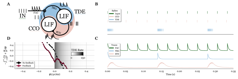
We propose here a Spiking Neural Network (SNN) model, the Spiking Phase-Locked Loop (sPLL), that interacts with the spectral footprint of sequences of input spikes, instead of using the average interspike interval. The model comprises two building blocks, the Time Difference Encoder (TDE)and the Current Controlled Oscillator (CCO), interacting in a closed loop. A detailed analysis of the model blocks is presented in Sec. 4.3. The model is depicted in Figure 1(A).

In this section we present the sPLL response to an input spike train with a fixed rate (i.e., single input frequency), and we demonstrate that our model successfully locks to the input frequency. The spiking activity of the two sPLL building blocks is illustrated in Figure 1(B). The frequency sensitivity of the sPLL is determined by the current $I_{\mathrm{bias}}$.

The three spiking neurons represent the INPUT, the TDE response and the CCO response. The frequency of the TDE is proportional to the phase difference between the spikes of the INPUT and the spikes of the CCO. The latter’s frequency is determined by a stable input current $I_{\mathrm{bias}}$ as well as by the synapse connected to the TDE. The spikes of the INPUT and CCO exhibit a tonic spike regime (i.e., the spikes are evenly distributed across time), while the TDE spikes in bursts (i.e., the spikes are concentrated in a small period of time).

In Figure 1(C), the traces of the synapses connecting the INPUT, the CCO, and the TDE are depicted. As mentioned in Sec. 4.3, the Facilitatory Trace (FAC) and Trigger Trace (TRG) do not integrate multiple stimuli ($f_{CCO}\ll 1/\tau_{\mathrm{TRG}}$, $f_{IN}\ll 1/\tau_{\mathrm{FAC}}$), while the Synaptic Trace (SYN) is integrating multiple spikes ($f_{TDE}\approx 1/\tau_{\mathrm{SYN}}$). This allows the two components of the sPLL to work in two different regimes. The TDE responds to one combination of input spikes per time (one from the FAC, one from the TRG) using multiple spikes, coding for the time difference between them. The CCO integrates multiple spikes coming from the TDE but outputs a single spike.

Figure 1(D) shows the potential well visualization, which illustrates how the sPLL locking mechanism works. In the example at hand the sPLL responds to an input frequency of $36\text{\,}\mathrm{Hz}$ and an input current with magnitude $40$ (normalized current). The red and black lines indicate the case where the feedback is present or absent respectively (i.e., the TDE does or does not communicate with the CCO).

In the figure we can see that, when the feedback is off, the phase is integrated periodically. This causes the TDE to respond with alternating high and low firing rate, which does not effectively encode information about the input firing rate. This is illustrated by the black line passing between different level of shaded background, indicating different TDE spiking activity. By contrast, when the feedback is on, the TDE response is fed back to the CCO. As a result, a local minimum (i.e., a stable state) emerges in the potential landscape, which allows the system to effectively lock to the input frequency.

Intuitively, when $\phi<0$, the inherent frequency difference forces $\phi$ to increase towards $0$, whereas if $\phi>0$, the spikes from the TDE cause the CCO frequency to increase, decreasing $\phi$ towards $0$. It is evident that regardless of the starting point, the system will eventually reach this state.

Note that, however, since the TDE behaves complementary to the phase difference (its activity is maximal when $\phi=0$), the observed behavior is not that of a pure stable state at $\phi=0$ (as would happen in a typical PLL). The sPLL alternates between being slightly above and slightly below $\phi=0$, as depicted by the system transitioning between high TDE spike counts and no TDE spikes in Figure 1(B).

Figure 2: sPLL layer processing data from PC afferents. Panels A and B reproduce the plots depicted in Figure 2 of [4]. The plots consists of real recordings of PC afferents, obtained from a Macaque sliding its finger on different textures and kindly provided by the authors. Panel A is a raster plot while panel B is a normalized FT. The different lines indicate different trials. Panel C illustrate the response of a layer of sPLL to the recorded spikes, coded in overall spike counts of the TDEs. Panel D depicts the FFT curves for the CCO in the sPLL layer with the lowest TDE spiking rate in panel C. The sPLL with the lowest activity has a spiking frequency consistent across trials. In panel E a normalized FFT of a selected input spike train for the texture ‘Hucktowel’ has been plotted. It is easy to observe that the spectral footprint of the ‘Hucktowel’ texture (depicted as a black line at the top of the figure) has a peak around $160\text{\,}\mathrm{Hz}$. The lower part of this panel shows the FFT of all the CCOs in response to the input spikes for ‘Hucktowel’. The color is derived from panel C, where each CCO is linked to its TDE. Panel F summarizes the test accuracy for a classifier trained on the spike count of the input spikes, the frequency footprint of the input spikes and the output activity of the TDEs. As we can see, while the spike count does not help in decoding the texture, the sPLL spike count and the FFT exhibit similar performance.

2.2 A Layer of sPLLs

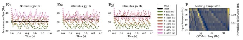
Given the sPLL’s ability to lock onto specific frequencies, we can leverage this paradigm to detect the main frequency of a spike train. To illustrate this, we constructed a layer of 50 sPLLs where each element has a distinct $I_{\mathrm{bias}}$ (ranging from $1260$, normalized current). When we feed an input spike train at a specific intrinsic frequency, the various sPLLs respond differently. This is evident in Figure 1(E1-E3), where the dots represent the instantaneous rate for every individual spike. The black dots represents the input spike train, while different colors represent different sPLLs.

The three input stimuli ($30\text{\,}\mathrm{Hz}$, $33\text{\,}\mathrm{Hz}$, $36\text{\,}\mathrm{Hz}$) interact differently with various CCOs based on the CCO’s intrinsic frequency (as defined by its input current $I_{\mathrm{bias}}$). CCOs that do not lock periodically change their frequency, following the phase accumulation between their intrinsic frequency and the input frequency (similar to what occurs in the potential well example in Figure 1(D) when no feedback is present). This behavior is visible in Figure 1(E1), where higher frequencies display a periodic behavior dictated by phase accumulation.

The sPLLs that manage to lock to the input do not accumulate phase. This results in a stable phase difference and consequently a more regular TDE spike activity. It’s noteworthy that several CCOs can lock to an input frequency due to the feedback loop that adjusts the internal frequency. This can be understood by examining the spread of the potential well in Figure 1(D) for the case with active feedback.

The distinct activity of the TDE can be utilized to easily identify the sPLLs that managed to lock more effectively. This is apparent in Figure 1(F), where the overall spike count of the TDE is plotted versus input frequency and versus CCO intrinsic frequency. The spike count of the TDE when receiving an input spike train was normalized over the input stimulus and over the intrinsic frequency of the CCO for clarity. The normalization can be justified by considering that a Winner-Takes-All (WTA) layer could be placed at the output of the sPLL network. The plot demonstrates that for any given input frequency, compatible with the investigated range of CCO intrinsic frequencies, there is an sPLL that is able to lock, leading to a low TDE spike count. The intrinsic frequencies of the CCO (the ticks of the x-axis in Figure 1(F)) were estimated by allowing the sPLL to run without an input stimulus (so the CCO was not excited by the synapse but only by the $I_{\mathrm{bias}}$).

Another observation in Figure 1(F) is that, close to each locking sPLL, there is another sPLL that spikes intensively. This is because when two spike trains have a low frequency difference, but not low enough to lock, or only lock poorly, the TDE spends a lot of time residing in the region where the firing rate is high, as visible in Figure 1(D).

Additionally, Figure 1(F) highlights the harmonics of the input signals. The sPLL doesn’t only lock with the input frequency but also with its multiples. This is mainly due to different harmonics of spike rate not being discernible because lower frequencies could be interpreted as higher frequency spike trains with missing spikes.

2.3 Modeling the somatosensory pathway

As explained in the introduction, the hypothesis of the existence of a phase-locked loop in the somatosensory pathway was proposed by Ahissar in the late ’90s [7]. The model presented there identified the cortex as the location of an oscillator, coupled with a phase detector in the thalamus.

Figure 3: In scheme A, B, C the four networks under test: 1 layer of 50 sPLL, 1 and 2 layers of 50 R-LIF, and a LSTM composed of 2 layers with output dimensionality of 50. All the networks are then passed through a linear classifier. In panel D the test accuracy over training of the four networks. The networks were tested against a linear classifier applied to the input spike count. The plot is composed of 15 different instances per network, with the mean plotted over it. In table E is shown the comparison among the different networks in terms of accuracy and in terms of resources (number of synapses and total spikes). The LSTM figure has been adapted from [15] under license CC BY-SA 4.0.

The sPLL described in Sec. 4.3 provides novel hypotheses about the biological somatosensory pathway. To quantitatively assess the similarity between the response of our model and biological data, we compare the sPLL response to in-vivo recordings of peripheral [4] and cortex [5] data from rhesus macaques.

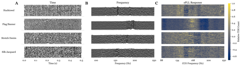
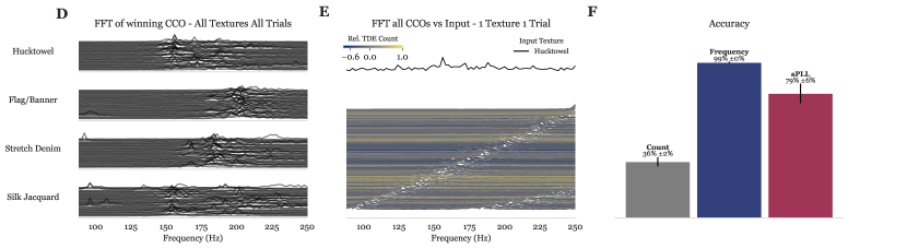
In Figure 2 (A and B) we recreated the peripheral recording depicted in Figure 2 from [4], using the PC response data kindly provided by the authors.

The figure shows data for 4 textures, with 63 trials each. The first part of the Figure illustrates the raster plots of the PCs response (Figure 2 (A)). Despite the nontrivial task to discriminate textures based on the raster plots (e.g. stretch Denim vs silk Jacquard) by visual inspection, it has been demonstrated that macaques are able to discriminate different textures of this kind when sliding their finger on them [6].

To characterize the frequency components of the PC response, we performed an FT analysis to extract the power spectrum from the neural recording data (see Fig. 2 (B)). One can qualitatively observe that, in contrast to the raster plots, the power spectrum of the spikes clearly provides footprints for different textures, with very low trial-to-trial variability.

To numerically assess this qualitative observation, the authors in [4] studied the correlation of both the mean firing rate and power spectra data with the input textures, demonstrating the superiority of frequency-based methods in decoding fine textures.

The similarity between our model and the afferent pathway projecting from the peripheral nerves was then studied by looking at the response of the sPLL to PC spiking activity. The experiment employed 200 sPLLs in parallel, all fed with different currents, driving the different CCOs in a range between $50\text{\,}\mathrm{Hz}$ and $125\text{\,}\mathrm{Hz}$. The biological data from [4] were presented as input for 2 seconds. The response of the TDE was then recorded over the experiment for all the different sPLLs.

In Figure 2(C), we report the results of the experiment. The x-axis depicts the frequencies at which the different CCOs are spiking, while the y-axis reports different trials. The color indicates the total spike count of the TDEs during the experiment. A normalization has been applied to acount for the intrinsic frequency difference between sPLLs. This normalization model fit a line to the intrinsic dependence between the $I_{\mathrm{bias}}$ and the TDE spike count, removing it for a fair comparison between sPLLs.

The sPLL response demonstrates a clear texture selectivity and low trial-to-trial variability. The locking behavior of the sPLL, as explained in Section 4.3, is expressed by regions of reduced response (shown in orange in Figure 2(C)) surrounded by enhanced response (in purple). These regions are closely related to the power spectrum peaks present in the PC activity (Figure 2(B)).

In order to quantify the performance of the sPLL model at detecting frequencies, we trained a linear classifier to predict the input texture on the basis of the data illustrated in Figure 2(A-C).

The classifier was trained on three different datasets. The first was the spike count in Figure 2(A), where the network first randomly projected to 200 neurons and then a linear classifier decoded it. The second was instead tested on the FFT of the spikes with a window of $200\text{\,}\mathrm{Hz}$. The third was trained using the outputs of the 200 sPLLs.

Figure 2(F) shows that the accuracy of the classifier is low when using the PC spike count ($36\text{\,}\mathrm{\char 37\relax}$), while it is high when using the power spectrum ($99\text{\,}\mathrm{\char 37\relax}$). The sPLL response produces an accuracy closer to that of the FFT, demonstrating that it can extract the spectral footprint ($81\text{\,}\mathrm{\char 37\relax}$). This result suggests that the sPLL model is a suitable candidate for the identification of the neural substrate of texture perception.

In Figure 2(D-E) we show the behaviour of the CCOs in response to different inputs, in order to compare it to what biological literature reports [5].

Starting from Figure 2(E), the FFT of a single trial of the Hucktower texture is presented, along with the FFTs of 200 different CCOs. In the top part the Hucktower texture FFT is shown as a single black line, while the rest of the plot is occupied by the FFT of the CCOs responding to the texture spikes. Every FFT is normalized with respect to its maximum and shifted according to the index of the CCO to have an informative view of the different trials. The color codes the overall spike count for the corresponding TDE, extracted from Figure 2(C), where blue indicates low activity, and yellow indicates high activity. Low activity in the TDE, usually associated with the locking behaviour, can be found in the frequency range comparable to the input frequency peak (around $80\text{\,}\mathrm{Hz}$) and in the harmonics associated with the peak (around $160\text{\,}\mathrm{Hz}$). This plot suggests that the TDE activity reflects the position of the CCO with the behaviour closest to the input frequency. This can be used to identify the frequencies at which the PC afferents spike, thanks to the locking of the CCO.

Figure 2(D) shows the FFT of the CCO associated with the TDE with the lowest spiking activity for multiple inputs and trials, following the method as used for Figure 2(E). One can see that, for a given texture, the behaviour of the CCOs is associated with the spectral footprint of the input. This result is in accordance with the experimental observation published in [5]. In said paper, cortex neurons projecting from PC afferents exhibit very consistent spectral footprints in response to input stimuli across trials, as visible in the reference’s Figure 3(E) in the supplementary material.

The results presented here suggest that the developed model of the sPLL has several points in common with the biological recordings performed in [4] and [5]. First we demonstrated that our model is able to decode the frequency footprint present in the spikes more efficiently than a simple spike count and with results comparable to an FFT. After this, we showed, in Figure 2(D), that the behaviours exhibited by components of our models can be similar to those demonstrated in the biological counterparts.

2.4 Multiple frequency decoding

After having shown that the sPLL can decode complex spectral footprints from biological spike trains, we explore the possibility of using this ability to perform computation in artificial agents, where complex spike patterns could be used to carry more variables in the same spike train. This possibility is discussed in Section Fourier Transform and Interspike Interval in the Supplementary Material, where Multifrequency Spike Train (MST) are decoded through the Interspike Intervals (ISIs) and FFTs.

Regarding the implementation of architectures for decoding MST,  [16] proposed an algorithm that processes spike trains using a Spike-based Low Pass Filter (S-LPF) bank emulating the cochlea’s frequency decomposition. The S-LPF is composed of a closed loop architecture made of a Hold & Fire (H&F), a Integrate & Generate (I&G) and a Spike Frequency Divider (SFD). The output of each S-LPF is a spike train where the spikes of a specific frequency have been removed. This algorithm therefore returns a bank of spike trains, in which each bank represents the spiking activity of the input, decomposed in a specific frequency range. The model used here, despite using spikes, heavily bases its functionality on clocked signals, due to the way it handles the individual events. This is a drawback when handling sparse time series as spike trains because it makes difficult to harness the low power computation of event-driven design.

To test the ability of the sPLL to detect multiple frequencies in a spike train, we performed a classification task where the inputs were composed of complex spike trains with two nested frequencies in it. The first frequency ($F_{1}$) was swept between $30\text{\,}\mathrm{Hz}$ and $54\text{\,}\mathrm{Hz}$, while the second frequency was swept between $30\text{\,}\mathrm{Hz}$ and $57\text{\,}\mathrm{Hz}$ as depicted in Figure S1(A) (explained in the Methods). Using this dataset, we compared our architecture with other notable architectures.

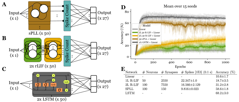
We first built a network composed of 50 sPLLs with progressive $I_{\mathrm{bias}}$ and shared input. The input was connected to the FAC terminal of each sPLL, as visible in Figure 3(A). The output of the sPLL network was then recorded over time and the total spikes during the simulation of each TDE were counted. This spike count was then used to train and test a linear classifier.

We then created two D-SNN networks of r-LIFs as explained in Sec. 4.4. One network was only composed of 50 neurons, connected in a one-to-all fashion to the input. They were then recurrently connected to the other neurons of their layer. Their spikes were counted and the resulting vector used for training a linear classifier. The training was acting both on the weights of the linear classifier as well as on the weights of the r-LIFs network. In the case of two layers of neurons, a second layer of 50 r-LIFs was introduced, as visible in Figure 3(B). In this case the training modified also the weights of the second layer.

To define the low and high boundaries of the accuracy we introduced two other networks: a simple linear classifier and a LSTM. The LSTM was composed of 2 layers with an output dimensionality of 50. The hidden state of the LSTM $h$ was used as input to a linear classifier. We found that the simple linear classifier applied to the spike count of the input was not enough to discern different frequencies whereas the LSTM (Figure 3(C)) showed a very good accuracy.

The results of the simulation are presented in Figure 3 (plot D and table E). The former depicts the test accuracy over epochs, while the latter summarizes the figures of merits. As we can see, the sPLLs layer performs closely to the LSTM, while the two networks made of R-LIF struggle to detect the different frequencies.

This is especially striking when comparing the resources. The sPLL is composed of two neurons and three synapses per element. This means that for the overall network there were 100 neurons and 150 synapses. The single layer R-LIF is composed of 50 neurons, where each neuron is connected to the input and to the other neurons in the layer for a total of 2550 plastic synapses. For the same reason, The 2 layer R-LIF has 100 neurons and 7550 plastic synapses.

Furthermore, the number of spikes generated by the sPLL is lower than the two D-SNNs, as can be seen in Figure 3(table E). This is due to the fact that the sPLL needs few spikes to abstract the overall spectral footprint of the stimulus, while the D-SNN requires more spikes to capture the temporal dynamics, and thus to be able to effectively decode the proposed input. The number of spikes has been chosen as a metric here because in artificial agents it often dictates the power consumption. This is due to the fact that the event generated by the spike is responsible for triggering a change, increasing the power consumption over time. Typical energy measures for such events are in the order of - in neuromorphic processors [17, 18, 19], giving us a reasonable estimate of the power consumption of one inference. Besides the lower overall spike count, the standard deviation for the total spike count is lower in case of the sPLL as well, which can be attributed to the fact that for the D-SNN the full network was trained with backpropagation, whereas in the sPLL only the linear classifier at the end was part of the training.

This result is striking because it shows that our model can accurately detect the frequencies in a multi-frequency signal better than complex SNNs composed of recurrent connections and trained using backpropagation, while maintaining a low and fixed connectivity pattern and sparse firing activity.

Importantly, it highlights how recurrent D-SNN are more suited for simple spiking patterns and are not fit for the case where a spike train is composed of multiple elements.

3 Conclusion

In this paper, we presented a novel model for a spiking neural network, the Spiking Phase-Locked Loop (sPLL), inspired by a previous work on phase-locked loops in the somatosensory cortex. We illustrated how the model works in simulation, highlighting how the sPLL manages to lock to an input frequency and how to use this behaviour to decode input frequencies.

We then presented the similarity between our model and biological data, hypothesizing that we proposed a good candidate for modeling the brain’s micro-circuitry: the sPLL is able to decode the texture represented by spike trains recorded from peripheral nerves in-vivo (Macaque data [5]), and the activity of the oscillator inside the model (the CCO) resembles recordings from cortical neurons projecting from PC afferents.

Moreover, we illustrated our model’s capability to decode multiple frequencies contained within a complex spike train. This feature positions the model as a promising candidate for advancing artificial touch and endowing artificial agents with unprecedented capabilities.

For future works, the possible paths to take are several, both towards improved SNNs, biological resemblance, and real-life applications.

We showed that our model functions as an essential component within a SNN, decoding frequency components in spike trains. In this regard, our model can be seamlessly integrated as a layer within the SNN architecture. A PyTorch module of the model is available for this purpose in the public repository at github.com/bics-rug/sPLL

Also, the sPLL paradigm could be harnessed for a novel method of information transmission across layers: a single spike train can convey multiple variables on multiple channels, distinguished by differing frequency bands, reminiscent of frequency-modulation encoding. Sets of sPLLs could exhibit sensitivity to specific frequency ranges and be able to capture information within these ranges, thereby facilitating a more streamlined communication channel.

Regarding biological resemblance, our model could have a deeper level of similarity to biology than what was explored here. A key feature of texture perception in biology is the independence from sliding speed. Our model can naturally be extended to exhibit this property. In fact, the $I_{\mathrm{bias}}$ current that defines the intrinsic frequency of every CCO can be adjusted, moving the selectivity of frequencies of a given sPLL to a different range. In a closed loop system with proprioception, this current can be dynamically modulated by the sliding speed. This approach would be coherent with the scheme proposed in [20], where the motor cortex (responsible for the sliding velocity) is projecting to the somatosensory cortex, informing it about the current strength applied to the muscles.

Another important extension of this work is to make our model compatible with applications relevant for artificial agents. In particular, an artificial agent used to assess the quality of fabrics may be given the task of decoding the perceived texture. In this scenario, data would be converted from analog pressure signals into spikes using transducers equivalent to the PC corpuscles, and the motor information would then be fed to the sPLLs.

For this purpose, a Complementary Metal Oxide Semiconductor (CMOS) circuit could be developed to decode tactile stimuli. Implementing this would be straightforward, given the documented existence of CMOS equivalents for all the constituent building blocks [21, 22, 23, 24]. In this scenario, the integrated circuits could be embodied into robots or prosthetics, enhancing the ability of artificial agents to discern textures, alongside other sensory stimuli such as vision and audio [25], while maintaining extremely low power consumption and minimal latency [26]. Currently, a realized CMOS circuit implementing these functions has been built and tested but is yet to be made publicly available.

4 Models

In this section we introduce the computational models used in this work. We first talk about the novel network proposed here, the Spiking Phase-Locked Loop (sPLL), along with the parts of which it is composed: the Current Controlled Oscillator (CCO)and the Time Difference Encoder (TDE). After that, we talk about the Deep Spiking Neural Network (D-SNN)and the Long Short-Term Memory (LSTM), used to compare the novel network with State-Of-The-Art (SOTA).

4.1 Current Controlled Oscillator

The Current Controlled Oscillator (CCO)is an oscillator that changes its frequency in relation to an input current. In this work, this is realized with a Current Based Leaky Integrate and Fire (CUBA-LIF), comprised of an integrating synapse and an integrating neuron.

The synapse can be represented by the following differential equation:

$$\frac{dI_{\mathrm{syn}}}{dt}=\frac{-I_{\mathrm{syn}}+\sum_{j}\mathrm{gain}_{\mathrm{syn}}\cdot\mathrm{spk}_{\mathrm{in}}^{j}}{\tau_{\mathrm{syn}}}$$ (1)

where:

• $I_{\mathrm{syn}}$ is the internal state of the synapse;

• $\mathrm{gain}_{\mathrm{syn}}$ is the voltage-to-current conversion factor;

• $\mathrm{spk}_{\mathrm{in}}$ represents the input spike (voltage);

• $\tau_{\mathrm{syn}}$ is the synapse time constant

Upon receiving a spike from a neuron, the synapse’s internal variable (representing a current) increases by $\mathrm{gain}_{\mathrm{syn}}/{C_{\mathrm{syn}}}$, and slowly decreases with a time constant of $\tau_{\mathrm{syn}}$.

The relationship between the input spike rate and the reached maximum current in this first-order differential equation can be obtained by considering the case in which a spike arrives either before or after the internal variable of the synapse is completely discharged. The formula for this would be:

$$I_{\mathrm{syn}}^{\mathrm{max}}\approx\begin{cases}\frac{\mathrm{gain}_{\mathrm{syn}}}{C_{\mathrm{syn}}}&\mathrm{if}\ f_{in}\ll\frac{1}{\tau_{\mathrm{syn}}}\\ \frac{\mathrm{gain}_{\mathrm{syn}}}{C_{\mathrm{syn}}}Ne^{-\frac{1}{f_{in}\tau_{\mathrm{syn}}}}&\mathrm{else}\end{cases}$$ (2)

where $f_{\mathrm{in}}$ is the frequency of the input and $N$ is the number of spikes that have occurred ($T_{\mathrm{sim}}$/$f_{\mathrm{in}}$). This means that if the internal variable of the synapse was not fully discharged before the arrival of the next spike the internal variable sums the contribution of multiple spikes.

The neuron, specifically a LIF model, follows a similar equation to that of the synapse, with the difference being that when the variable $V$ exceeds a threshold, it resets to $0$ for a refractory time $T_{\mathrm{refr}}$:

$$\begin{cases}\frac{dV_{\mathrm{mem}}}{dt}=-\frac{V_{\mathrm{mem}}}{\tau_{\mathrm{neu}}}+\frac{I_{\mathrm{in}}}{C_{\mathrm{mem}}}\\ \mathrm{if}\ V>V_{\mathrm{thr}}\ \&\ \mathrm{count_{refr}}=0\rightarrow\mathrm{spk}\\ \mathrm{if}\ \mathrm{spk}\rightarrow\mathrm{count_{refr}}=T_{\mathrm{refr}},\ V=0\\ \mathrm{if}\ !\mathrm{spk}\rightarrow\mathrm{count_{refr}}=\mathrm{count_{refr}}-1\end{cases}$$ (3)

where $I_{\mathrm{in}}$ is the input current fed to the neuron, which can originate from a synapse or a stable current input:

$$I_{\mathrm{in}}=I_{\mathrm{syn}}+I_{\mathrm{bias}}$$ (4)

Assuming a constant current at the input, and solving the first-order differential equation, we can estimate the time when the neuron reaches the threshold as:

$$\begin{cases}t_{\mathrm{thr}}=\tau_{\mathrm{neu}}\ln\left(\frac{I_{\mathrm{in}}}{I_{\mathrm{in}}-\frac{C_{\mathrm{mem}}}{\tau_{\mathrm{neu}}}V_{thr}}\right)\\ t_{\mathrm{thr}}=T_{\mathrm{refr}}&\mathrm{if\ t_{\mathrm{thr}}>T_{\mathrm{refr}}}\end{cases}$$ (5)

Given that the frequency of a neuron is defined as the average ISI, we can say that $f_{\mathrm{neu}}=1/t_{\mathrm{thr}}$. Note that the frequency of the neuron is capped by the refractory period. By imposing that the neuron is controlled by a constant current, we have thus created a CCO using a simple neuron.

4.2 Time Difference Encoder

The Time Difference Encoder (TDE)is a model used in neuromorphic computing to translate the time difference between two input spike trains into a spike rate [24, 27, 28, 29], which consists of a gated synapse and a neuron. The gated synapse is composed of two traces, FAC and TRG, as illustrated in Figure 1, where the gating is graphically represented with a ring around the TRG. Both FAC and TRG are similar to the trace presented in Eq. 1, except for the modulation of TRG’s $\mathrm{gain}_{\mathrm{syn}}$ by FAC.

$$\begin{cases}\frac{dI_{\mathrm{FAC}}}{dt}=-\frac{I_{\mathrm{FAC}}}{\tau_{\mathrm{FAC}}}+\frac{{\mathrm{gain}_{\mathrm{FAC}}\mathrm{spk}_{\mathrm{FAC}}}}{C_{\mathrm{FAC}}}\\[10.0pt] \frac{dI_{\mathrm{TRG}}}{dt}=-\frac{I_{\mathrm{TRG}}}{\tau_{\mathrm{TRG}}}+\frac{{\mathrm{gain}_{\mathrm{TRG}}I_{\mathrm{\mathrm{FAC}}}\mathrm{spk}_{\mathrm{TRG}}}}{C_{\mathrm{TRG}}}\end{cases}$$ (6)

As demonstrated in [30], we can estimate that the current of the TRG depends on the time difference between the spikes’ arrival time from the two channels (defined here as $t_{TRG}$ and $t_{FAC}$) and on the gain of both the FAC and the TRG.

$$I_{\mathrm{{TRG}}}(t)=\begin{cases}I_{\mathrm{gain}}e^{-\frac{\Delta t}{\tau_{\mathrm{FAC}}}}e^{-\frac{t-t_{\mathrm{TRG}}}{\tau_{\mathrm{TRG}}}}&\mbox{if $\Delta t>0$}\\[6.0pt] 0&\mbox{else}\end{cases}$$ (7)

where $\Delta t=t_{\mathrm{TRG}}-t_{\mathrm{FAC}}$ and $I_{\mathrm{gain}}=I_{\mathrm{gainFAC}}I_{\mathrm{gainTRG}}$.

The TRG current is then fed into a LIF neuron, which responds with spikes related to the time difference between the FAC and the TRG channels. In the end, assuming a logarithmic dependence between the spiking activity and the current, and an exponential dependence between the current and the time difference, the frequency of the TDE is given by:

$$f_{\mathrm{tde}}\propto\frac{1}{t_{\mathrm{TRG}}-t_{\mathrm{FAC}}}$$ (8)

Note that this last approximation assumes that the TDE’s traces are at their minimum every time an input spike arrives at both the TRG and FAC. This is possible if the input frequencies are lower than the reciprocal of the model’s $\tau$s ($f_{in}\ll 1/\tau_{FAC},1/\tau_{TRG}$), as visible in Eq. 2.

4.3 Spiking Phase-Locked Loop

This model, known as the Spiking Phase-Locked Loop (sPLL), was initially introduced in [31], inspired by previous works in [7]. It comprises a CCO and a TDE arranged in a feedback loop, as depicted in Figure 1(A).

The model functions as follows: the CCO receives a stable current from an external terminal ($I_{\mathrm{bias}}$), inducing spiking at a specific frequency. The TDE receives spikes from the input via the FAC terminal and from the CCO through the TRG terminal. Subsequently, the output of the TDE is channeled to a synapse that stimulates the CCO. This stimulation results in the adjustment of the operating frequency of the CCO. The variation in frequency is subsequently employed to minimize the phase differential between the input and the phase of the CCO.

As illustrated in Figure 1(A), the spikes are integrated into currents using synapses (due to the Current Based (CUBA) property), which then feed into the subsequent neuron. This method is used convert voltage signals (the spikes) into current signals (the traces) and to give temporal kernels to the spikes.

The equation governing the sPLL is an interacting version of the two models: the CCO and the TDE. As explained in the TDE section, if we consider that the frequency of the INPUT and the frequency of the CCO are both lower than the reciprocal of the TDE’s $\tau$s, we can utilize Eq. 8. Conversely, if we assume that the input frequency of the CCO is higher than the reciprocal of its $\tau$ but still lower than the reciprocal of the threshold period $\frac{1}{T_{\mathrm{refr}}}$, we can state that:

$$f_{\mathrm{cco}}\propto\ln\left(\frac{I_{in}}{I_{in}+\frac{C_{\mathrm{mem}}}{\tau_{\mathrm{neu}}}V_{\text{thr}}}\right)\approx\ln\left(\frac{I_{in}}{\frac{C_{\mathrm{mem}}}{\tau_{\mathrm{neu}}}V_{\text{thr}}}\right)$$ (9)

Considering now that the TDE has a spiking rate comparable to $\tau_{\mathrm{SYN}}$ we can say that:

$$I_{\mathrm{SYN}}=\frac{\mathrm{gain}_{\mathrm{syn}}}{C_{\mathrm{syn}}}Ne^{-\frac{1}{f_{in}\tau_{\mathrm{syn}}}}$$ (10)

where N is the number of spikes emitted by the TDE. So we have that:

$$f_{\mathrm{cco}}\propto\frac{ln\left(N\right)}{\tau}\approx\frac{N}{\tau}\approx f_{\mathrm{tde}}$$ (11)

Now, assuming that the spike trains are periodic ($t_{\text{spike}}=\phi_{\text{spike}}$), we can further deduce:

$$\begin{cases}f_{\text{tde}}\propto\phi_{\text{cco}}-\phi_{\text{in}}\\ f_{\text{cco}}\propto f_{\text{tde}}\\ \phi_{\text{cco}}=\int f_{\text{tde}}\end{cases}$$ (12)

Here, $\phi_{\text{cco}}$ and $\phi_{\text{in}}$ represent the phases of a given spike in the CCO and INPUT, respectively.

4.4 Deep Spiking Neural Network

To compare the performance of the sPLL, we opted for the most common neuromorphic algorithm for classification: a Deep Spiking Neural Network (D-SNN). This network consists of several layers (either 1 or 2 hidden layers in this work) of LIF neurons interconnected using integrating synapses (CUBA-LIF).

In this architecture, each neuron communicates with the subsequent layer and within its own layer through an all-to-all connection, thus forming a Recurrent Neural Network (RNN) of R-LIF. We utilized Backpropagation Through Time (BPTT) and surrogate gradients to train the input synapses of every layer, as well as the recurrent ones.

4.5 Long Short-Term Memory

We also employed an algorithm suited for temporal datasets to benchmark the sPLL against the traditional SOTA: Long Short-Term Memory (LSTM). This model, first introduced by [32], represents an improvement over traditional RNNs, effectively addressing the vanishing gradient problem.

The LSTM model, depicted in Figure 3(C), consists of a complex unit named a memory cell, that stores the time sequence used for computation. It comprises three gates: the input gate, the output gate, and the forget gate. These gates play a crucial role in regulating the information stored in the memory cell. The forget gate decides which existing information in the memory cell should be discarded, the input gate determines which parts from the input should be retained, and the output gate defines which portions of the stored values should be propagated to the output.

In this work, we utilized a two-layer LSTM with an input dimensionality of 1 and an output dimensionality of 50. The internal state $h$ was used as a vector for training a classifier. The parameters of the LSTM were trained using backpropagation.

5 Methods

5.1 Multifrequency Spike Trains

Neurons in neuromorphic systems communicate using digital voltage pulses with fixed height and width, known as spikes. The information transmitted between neurons can be encoded in the time difference between these spikes.

In the simplest case in which the time between spikes is constant over time, the spike train can be described by a Dirac comb:

$$R(t)=\frac{1}{T}\sum_{k}{\delta(t-kT)}$$ (13)

To account for noise and variability, we consider the formula:

$$R(t)=\frac{1}{T}\sum_{k}{\delta\left(t-\left(kT+\mu+\sigma[k]\right)\right)}$$ (14)

where $\mu$ is a random time shift that affects all the $\delta$s equally and $\sigma$ represents jitter noise which modifies the time of each spike independently.

More generally, spike trains differ from Dirac combs in that they do not have to be periodic, and each spike can have an arbitrary distance from the previous one. Thus, we define:

$$R(t)=\sum_{k}{\frac{1}{\mathrm{ISI}_{k}}\delta(t-t_{s}[k])}$$ (15)

where $t_{s}[k]$ is the time of the $k-th$ spike. The ISIs are defined as the time differences between consecutive spikes: $\mathrm{ISI}_{k}=t_{s}[k]-t_{s}[k-1]$. In case the spike train is generated from a Dirac comb with the addition of jitter noise the time of the $k-th$ spike is given by $t_{s}[k]=kT+\mu+\sigma[k]$.

Extending from the definition of a spike train, we consider spike trains with multiple frequencies, referred to as MSTs. They are created by merging spike trains with different frequencies:

$$R(t)=\mathrm{merge}(R_{0}(t),R_{1}(t))=\\ \frac{1}{T_{1}}\sum_{k}{\delta(t-t^{1}_{s}[k])}\ |\ \frac{1}{T_{2}}\sum_{k}{\delta(t-t^{2}_{s}[k])}$$ (16)

where each train $R_{i}(t)$ has its period $T_{i}$ and the temporal jitter is sampled from a Gaussian random distribution, e.g. $t^{i}_{s}[k]=kT_{i}+\mu_{i}+\sigma_{i}[k]$. The operation performed here, akin to an OR gate ($|$), merges the two spike trains into a single time series. Note that this means that when two spikes coincide, we consider them as a single spike, with the usual fixed height and width. Note that the merge operation creates a new spike train where the distance between spikes cannot be described using Eq. 13, but instead requires the use of Eq. 15.

5.2 Fourier Transform

In the software developed for this work, spikes are represented by ones in a tensor of zeros with the length of the tensor being as large as the simulation time multiplied by the sampling frequency (or simulation clock).

These spike tensors can be interpreted as continuous time-varying signals, in which case each individual spike cannot be described by a Dirac $\delta$ but needs to be associated to a specific width and a unitary height. This results in a sequence of rectangles ($\mathrm{rect}$) in time.

From this, the frequency composition of the spike train can be obtained by examining the spectral footprint generated by the FT, which would be impossible when using the Dirac $\delta$ representation.

5.3 Synthetic Dataset

To evaluate the performance of various algorithms at identifying different frequencies, we created a dataset of spike trains composed of two frequencies, each lasting $100\text{\,}\mathrm{ms}$, as depicted in Figure S1(A). The first frequency $F_{1}$ was varied between $30\text{\,}\mathrm{Hz}$ and $54\text{\,}\mathrm{Hz}$ with a step of $3\text{\,}\mathrm{Hz}$, while $F_{2}$ had the same range but a step of $9\text{\,}\mathrm{Hz}$, resulting in a total of 27 unique combinations. Each combination was created 100 times. Each spike train was affected by a temporal shift (randomly selected but fixed for each train, e.g. affecting all spikes equally) and jitter noise. The noise was sampled for every spike from a normal distribution:

$$\sigma(f,k)=\mathcal{N}(0,1)\frac{\mathrm{mag_{\sigma}}f_{N}}{f}$$ (17)

whereas the shift was computed as:

$$\mu(f)=\mathcal{N}(0,1)\frac{\mathrm{mag_{\mu}}f_{N}}{f}$$ (18)

with $\mathrm{mag_{\sigma}}$ = $100\text{\,}\mathrm{ms}$ and $\mathrm{mag_{\mu}}$ = $1\text{\,}\mathrm{ms}$. In these equations, $f_{N}$ is the Nyquist sampling frequency, $f$ represents the frequency of the spike train, and k is the index of the single spike.

The dataset was divided in training (2187 samples, 81%), evaluation (243 samples, 9%) and testing (270 samples, 10%). The distinction between training and evaluation was only present during hyperparameter optimization (Sec. 5.7).

5.4 Classifier

To assess the performances of the different algorithms against the syntethic dataset described above, a classifier was introduced. A linear layer of 27 output units was benchmarked with one-hot encoding (i.e, the label of the data is compared with the index of the most active neuron). The weights of the linear classifier were updated using traditional backpropagation, instructed by a cross-entropy loss [33].

Due to the one-hot encoding requiring a single output label, a strategy consisting of creating one class per frequency combination was selected, since compared to the usage of multi-label classifiers, this method offers the advantage of reducing the hyperparameters to be optimized (specifically the output activity threshold).

5.5 Backpropagation Through Time

In this work, specifically for the model’s multifrequency experiment, we trained the weights of the spiking neural networks. To do so we used Backpropagation Through Time (BPTT) [34], an algorithm for applying backpropagation to functions that have a temporal dynamics.

The BPTT algorithm first computes the activity of the neuron with a normal iterative process (in this work forward Euler), allowing for the simulation of the network of neurons. It then activates the backward pass, which consists of computing the error of the network through the loss function, after which the error is propagated back to the network’s elements. The algorithm saves all the time steps computed in the forward pass and propagates the gradient in the temporal domain, unfolding the network as if it was a multi-layer network (unroll).

In this work, the BPTT is automatically setup by the autograd function of Pytorch [35].

5.6 Surrogate Gradient

To train spiking neural networks we need to backpropagate the error computed with the loss function through the activity of the neurons. However, the spikes that neurons use to communicate cannot be differentiated. In this work we use the surrogate gradient proposed in [36] to overcome the problem. In this method, the spike is convoluted with a kernel composed of the normalized negative part of a fast sigmoid such that the gradient is

$$\nabla_{\mathrm{surrogate}}=\frac{\nabla_{\mathrm{in}}}{\left(a\cdot|\mathrm{spk}|+b\right)^{2}}$$ (19)

where $a=20$ and $b=1$, as used in [37]. Thanks to this operation, the algorithm can compute a continuous gradient in the backward pass, while simulating a normal spiking neuron in the forward pass.

5.7 Hyperparameter Optimization

The models used in this work (explained in Section 4) have several parameters that influence the performance of the network. For example, the D-SNN model presented in Sec. 4.4 has $\tau$s and gains that affect the frequency or the excitability of the neurons. To guarantee a fair comparison across models, we optimized the R-LIF networks using a hyperparameter optimization framework called Neural Network Intelligence (NNI) [38]. This program runs the desired script several times, while pursuing the maximum accuracy. In the NNI framework, the evaluation part of the dataset was used as testing.

For the D-SNN the NNI optimized $\tau_{\mathrm{syn}}$, $\tau_{\mathrm{neu}}$, $\mathrm{gain}_{\mathrm{syn}}$, $\mathrm{gain}_{\mathrm{neu}}$, $lr_{\mathrm{R-LIF}}$ and $lr_{\mathrm{dec}}$. The last two elements are the learning rate of the spiking neurons and the learning rate of the decoder, respectively. The algorithm was run 100 times using annealing. For the sPLL, no automatic optimization has been performed due to the manual optimization already performed in the past. For the LSTM, no optimization algorithm was used.

5.8 Potential Well Analysis

To gain insights on the sPLL behavior, we devised a model based on the concept of a potential landscape in phase space [39]. The potential $V(\phi)$ is defined with respect to the phase difference of the system (Sec. 4.3):

$$\phi=\phi_{\mathrm{IN}}-\phi_{\mathrm{CCO}}\pmod{2\pi}$$ (20)

such that $\phi$ is positive if the CCO spikes after the input IN. One can imagine to place a “phase particle” on this potential landscape and observe the evolution of the system. The “phase particle” would move in the energy landscape, seeking the minimum of the potential energy within the cyclic phase space.

An illustrative example of such a potential landscape is presented in Figure 1(D). To comprehend how this landscape was created, we first need to define several fictitious forces. The first force, $F_{\mathrm{freq}}$, is a constant term related to the intrinsic frequency difference between the CCO and the input IN:

$$F_{\mathrm{freq}}\propto f_{\mathrm{IN}}-f_{\mathrm{cco}}$$ (21)

However, this force alone would cause $\frac{d\phi}{dt}$ to tend to infinity, necessitating the introduction of a friction term, $C_{f}\frac{d\phi}{dt}$, where $C_{f}$ is an arbitrary constant. Finally, we introduce $F_{\mathrm{TDE}}$, a force modeling the behavior of the TDE, the spikes of which accelerate the CCO. This gives us the complete equation of motion:

$$m\frac{d^{2}\phi}{dt^{2}}=F_{\mathrm{freq}}-C_{f}\frac{d\phi}{dt}+F_{\mathrm{TDE}}$$ (22)

where $m$ is the “mass” of our phase particle, related to the dynamics of the CCO synapse. To find the potential, we integrate the conservative forces with respect to the phase $\phi$:

$$V(\phi)=-\int\left(F_{\mathrm{freq}}+F_{\mathrm{TDE}}\right)\ d\phi$$ (23)

As we cannot measure these forces directly however, we substitute Equation 22 to obtain:

$$V(\phi)=-\int\left(m\frac{d^{2}\phi}{dt^{2}}+C_{f}\frac{d\phi}{dt}\right)\ d\phi$$ (24)

Finally, Figure 1(D) was generated by simulating the model multiple times with varying initial conditions, and determining $\frac{d\phi}{dt}$ and $\frac{d^{2}\phi}{dt^{2}}$ for each run. Subsequently, all the data points were numerically integrated together.

Supplementary Materials

Instantaneous Rate Histogram

When analyzing the information contained in spike trains, a typical approach used in literature is the Instantaneous Rate Histogram (IRH). This algorithm computes the distribution of the time between each consecutive spike in the spike train.

Using Eq. 15, we can express it as follows:

$$R(t)=\frac{1}{\sum_{k}t_{s}[k]}\sum_{k}{\delta(t-t_{s}[k]+\sigma[k]+\mu)}\xrightarrow{ISI}t_{s}+\sigma[k]+\mu\xrightarrow{HIST}\mathrm{dist}(t_{s}+\sigma[k]+\mu)$$ (25)

Given a spike train with a specific frequency, the histogram of the reciprocal of the ISI, here defined as Instantaneous Rate Histogram (IRH), is likely to produce a Gaussian function around the spike train’s frequency (for example in Eq. 15 it is gonna reveal $mean(t_{s})$).

In the case of multiple frequencies, the resulting ISI creates a new $t_{s}$. Using a probability analysis, we can infer what the distribution of ISI looks like. Assuming two spike trains $R_{1}$ and $R_{2}$ with periods $T_{2}>T_{1}$, the likelihood of having a spike generated by $R_{1}$ is given by:

$$P(T_{1})=\frac{\alpha}{T_{1}}\left[\left(1-\frac{T_{1}}{T_{2}}\right)\delta(t-T_{1})+\frac{T_{1}}{T_{2}}\mathcal{U}(0,T_{1})\right]$$

The probability of having a spike generated by $R_{2}$ is given by:

$$P(T_{2})=\frac{\alpha}{T_{2}}\mathcal{U}(0,T_{1})$$

where $\alpha$ is such that $\alpha/T1+\alpha/T2=1$.

The resulting distribution comes out as:

$$P=P(T1)+P(T2)=\frac{2T_{1}}{T_{1}+T_{2}}\mathcal{U}(0,T_{1})+\delta(t-T_{1})$$ (26)

The histogram in this case gives a blurry picture about which frequencies were initially encoded in the spike trains. The histogram has been computed using the Numpy module’s histogram function.

Fourier Transform and Interspike Interval

Information about the internal state of the neuron is typically propagated using the reciprocal of the time difference between spikes, denoted as Instantaneous Rate (IR) ($\text{IR}=1/\text{ISI}$), as explained in Sec. 5.1. In this context, the neuron’s internal state at time $t$ is characterized by the reciprocal of the time difference between $\delta_{t}$ and $\delta_{t-1}$. The mean of IR provides the average neuron firing rate, thus informing about its the input signal.

However, when a spike train contains multiple variables to transmit, analyzing the single instantaneous rate might be insufficient. The time difference between every consecutive spike could be misleading, particularly when introducing the concept of $t_{s}$ in a merged spike train (as discussed in 5.1).

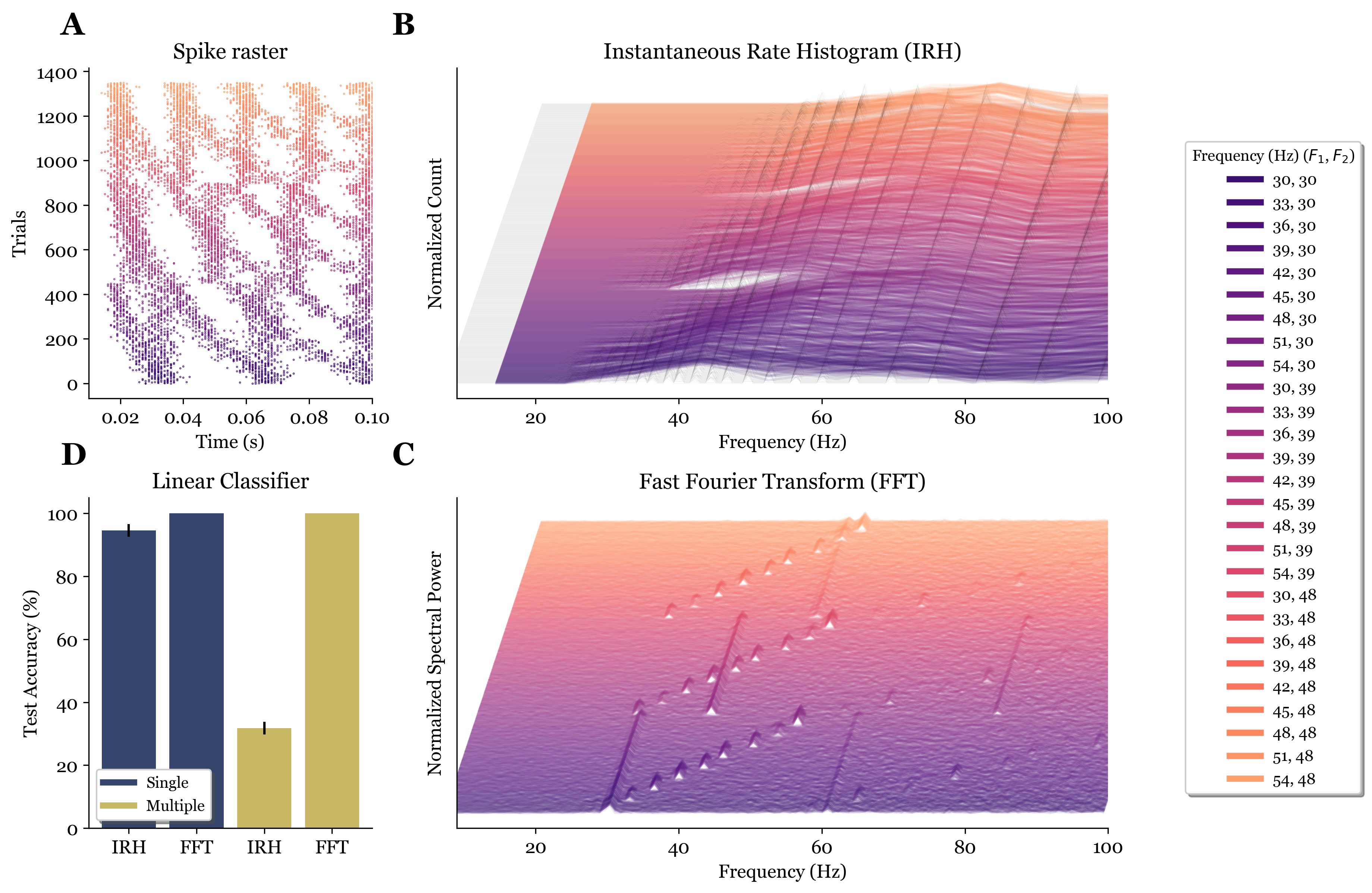
To investigate this, we conducted a benchmark comparing two different spike analysis methods: utilizing the IRH of the spike train and employing the FFT of the spike train (as explained in Sec. 5.2). The dataset used for this analysis comprises two frequencies with added jitter noise, representing two internal variables ($F_{1}$ and $F_{2}$), elaborated further in Sec. 5.3 and depicted in Figure S1(A).

For the IRH, we computed the time difference between each consecutive spike and then applied a histogram function. The results, depicted in Figure S1(B), exhibit an interplay between the two frequencies. The plot reflects the behavior outlined in Sec. 5.1, where for each frequency combination, the lowest frequency determines the minimum x-value of the histogram. Meanwhile, the upper part of the histogram is evenly filled with events due to the random shift between the two frequencies. It’s worth noting that introducing random jitter to both frequencies results in a Gaussian spread around the peak predicted by the equations. This outcome underscores the challenge of identifying the frequencies composing a given histogram, especially in the presence of random noise. Note that the black lines depict the histogram if 200 bins are used, while the colored lines depict the case for 10 bins. The 10 bins case has been used to improve readibility while the 200 bins case has been used to test against the FFT (explained further).

In contrast, Figure S1(C) portrays the same dataset analyzed using the FFT. Here, the spikes are considered as ones and the absence of spikes as zeros. The Fourier transform is able to consistently identify the original frequencies and distinguish the different contributions of the two internal variables. Harmonics of the frequencies are also visible.

To quantitatively test this hypothesis, we fed the outputs of IRH and FFT to a linear classifier for both the described dataset and a dataset with only one frequency (27 instances from $30\text{\,}\mathrm{Hz}$ to $54\text{\,}\mathrm{Hz}$). This was repeated by varying the random seed 15 times. Both the IRH and FFT had a dimensionality of 200. The classifier was trained with these data for 100 epochs as explained in Sec. 5.4. As illustrated in Figure S1D, for the single frequency example, both the FFT and IRH are able to discern the frequency in a comparable manner. This is because the interspike interval reflects the input frequency. However, when adding the second frequency to the input, the FFT algorithm can more reliably discern the different frequencies present in the dataset, while the IRH struggles. This can be attributed to the fact that merging several spike trains makes the interspike interval unreliable in determining the contained frequencies.

The primary contribution of this experiment is demonstrating that multiple variables can be encoded in a single spike train, with each variable’s value represented by a spiking frequency. We have demonstrated that standard procedures like IRH may not adequately extract or visualize this information, necessitating more complex analyses.

Figure S1: In panel A the raster plot of the dataset introduced in Sec. 5.3 is illustrated. In panel B the IRH for the dataset in A is shown with a bin number of 10. In panel C an FFT of the spike trains is computed for every trail with a sampling rate of $1\text{\,}\mathrm{k}\mathrm{H}\mathrm{z}$. Finally in panel D, the results of a linear classifier predicting the frequency composition in a single frequency and a double frequency case for 15 different seeds. Both the IRH and FFT have a dimensionality of 200.

References

- [1] Michael A. Muniak et al. “The Neural Coding of Stimulus Intensity: Linking the Population Response of Mechanoreceptive Afferents with Psychophysical Behavior” In Journal of Neuroscience 27.43 Society for Neuroscience, 2007, pp. 11687–11699 DOI: 10.1523/JNEUROSCI.1486-07.2007
- [2] Giulia Corniani and Hannes P. Saal “Tactile Innervation Densities across the Whole Body” In Journal of Neurophysiology 124.4 American Physiological Society, 2020, pp. 1229–1240 DOI: 10.1152/jn.00313.2020
- [3] Hannes P. Saal and Sliman J. Bensmaia “Touch Is a Team Effort: Interplay of Submodalities in Cutaneous Sensibility” In Trends in Neurosciences 37.12 Elsevier, 2014, pp. 689–697 DOI: 10.1016/j.tins.2014.08.012
- [4] Alison I. Weber et al. “Spatial and Temporal Codes Mediate the Tactile Perception of Natural Textures” In Proceedings of the National Academy of Sciences 110.42 National Academy of Sciences, 2013, pp. 17107–17112 DOI: 10.1073/pnas.1305509110
- [5] Justin D. Lieber and Sliman J. Bensmaia “High-Dimensional Representation of Texture in Somatosensory Cortex of Primates” In Proceedings of the National Academy of Sciences 116.8 Proceedings of the National Academy of Sciences, 2019, pp. 3268–3277 DOI: 10.1073/pnas.1818501116
- [6] Katie H. Long et al. “Texture Coding in Higher Order Somatosensory Cortices of Primates” bioRxiv, 2022, pp. 2022.08.19.504511 DOI: 10.1101/2022.08.19.504511
- [7] Ehud Ahissar “Temporal-Code to Rate-Code Conversion by Neuronal Phase-Locked Loops” In Neural Computation 10.3, 1998, pp. 597–650 DOI: 10.1162/089976698300017683
- [8] Harrison Nguyen et al. “Dynamic Texture Decoding Using a Neuromorphic Multilayer Tactile Sensor” In 2018 IEEE Biomedical Circuits and Systems Conference (BioCAS), 2018, pp. 1–4 DOI: 10.1109/BIOCAS.2018.8584826
- [9] E.M. Izhikevich “Simple Model of Spiking Neurons” In IEEE Transactions on Neural Networks 14.6, 2003, pp. 1569–1572 DOI: 10.1109/TNN.2003.820440
- [10] Mahdi Rasouli et al. “An Extreme Learning Machine-Based Neuromorphic Tactile Sensing System for Texture Recognition” In IEEE Transactions on Biomedical Circuits and Systems 12.2, 2018, pp. 313–325 DOI: 10.1109/TBCAS.2018.2805721
- [11] Mark M. Iskarous et al. “Unsupervised Learning and Adaptive Classification of Neuromorphic Tactile Encoding of Textures” In 2018 IEEE Biomedical Circuits and Systems Conference (BioCAS) Cleveland, OH: IEEE, 2018, pp. 1–4 DOI: 10.1109/BIOCAS.2018.8584702
- [12] Sriramana Sankar et al. “Texture Discrimination with a Soft Biomimetic Finger Using a Flexible Neuromorphic Tactile Sensor Array That Provides Sensory Feedback” In Soft Robotics 8.5 Mary Ann Liebert, Inc., publishers, 2021, pp. 577–587 DOI: 10.1089/soro.2020.0016
- [13] Ruihan Gao, Tasbolat Taunyazov, Zhiping Lin and Yan Wu “Supervised Autoencoder Joint Learning on Heterogeneous Tactile Sensory Data: Improving Material Classification Performance” In 2020 IEEE/RSJ International Conference on Intelligent Robots and Systems (IROS), 2020, pp. 10907–10913 DOI: 10.1109/IROS45743.2020.9341111
- [14] Tasbolat Taunyazov et al. “Fast Texture Classification Using Tactile Neural Coding and Spiking Neural Network” In 2020 IEEE/RSJ International Conference on Intelligent Robots and Systems (IROS), 2020, pp. 9890–9895 DOI: 10.1109/IROS45743.2020.9340693
- [15] Guillaume Chevalier “Long Short-Term Memory” In Wikipedia, 2023
- [16] Angel Jimenez-Fernandez et al. “A Binaural Neuromorphic Auditory Sensor for FPGA: A Spike Signal Processing Approach” In IEEE transactions on neural networks and learning systems 28.4, 2017, pp. 804–818 DOI: 10.1109/TNNLS.2016.2583223
- [17] Mike Davies et al. “Loihi: A Neuromorphic Manycore Processor with On-Chip Learning” In IEEE Micro 38.1, 2018, pp. 82–99 DOI: 10.1109/MM.2018.112130359
- [18] Charlotte Frenkel, Jean-Didier Legat and David Bol “MorphIC: A 65-Nm 738k-Synapse/Mm2̂ Quad-Core Binary-Weight Digital Neuromorphic Processor With Stochastic Spike-Driven Online Learning” In IEEE Transactions on Biomedical Circuits and Systems 13.5, 2019, pp. 999–1010 DOI: 10.1109/TBCAS.2019.2928793
- [19] M. Mastella et al. “Tunneling-Based CMOS Floating Gate Synapse for Low Power Spike Timing Dependent Plasticity” In 2020 2nd IEEE International Conference on Artificial Intelligence Circuits and Systems (AICAS), 2020, pp. 213–217 DOI: 10.1109/AICAS48895.2020.9073965
- [20] E. Ahissar and T. Oram “Thalamic Relay or Cortico-Thalamic Processing? Old Question, New Answers” In Cerebral Cortex 25.4, 2015, pp. 845–848 DOI: 10.1093/cercor/bht296
- [21] Chiara Bartolozzi and Giacomo Indiveri “Synaptic Dynamics in Analog VLSI” In Neural Computation 19.10, 2007, pp. 2581–2603 DOI: 10.1162/neco.2007.19.10.2581
- [22] Paolo Livi and Giacomo Indiveri “A Current-Mode Conductance-Based Silicon Neuron for Address-Event Neuromorphic Systems” In 2009 IEEE International Symposium on Circuits and Systems Taipei, Taiwan: IEEE, 2009, pp. 2898–2901 DOI: 10.1109/ISCAS.2009.5118408
- [23] Elisabetta Chicca, Fabio Stefanini, Chiara Bartolozzi and Giacomo Indiveri “Neuromorphic Electronic Circuits for Building Autonomous Cognitive Systems” In Proceedings of the IEEE 102.9, 2014, pp. 1367–1388 DOI: 10.1109/JPROC.2014.2313954
- [24] M.. Milde et al. “Spiking Elementary Motion Detector in Neuromorphic Systems” In Neural Computation 30.9, 2018, pp. 2384–2417 DOI: 10.1162/neco_a_01112
- [25] Ehud Ahissar et al. “Thalamocortical Loops as Temporal Demodulators across Senses” In Communications Biology 6.1 Nature Publishing Group, 2023, pp. 1–11 DOI: 10.1038/s42003-023-04881-4
- [26] Chiara Bartolozzi, Lorenzo Natale, Francesco Nori and Giorgio Metta “Robots with a Sense of Touch” In Nature Materials 15.9, 2016, pp. 921–925 DOI: 10.1038/nmat4731
- [27] Giulia Veronica D’Angelo et al. “Event-Based Eccentric Motion Detection Exploiting Time Difference Encoding” In Frontiers in Neuroscience 14, 2020
- [28] Thorben Schoepe et al. “Finding the Gap: Neuromorphic Motion Vision in Cluttered Environments” arXiv, 2021 arXiv:2102.08417 [cs]
- [29] Daniel Gutierrez-Galan et al. “An Event-Based Digital Time Difference Encoder Model Implementation for Neuromorphic Systems” In IEEE Transactions on Neural Networks and Learning Systems 33.5 IEEE, 2021, pp. 1959–1973
- [30] Hugh Greatorex et al. “On-Chip Event-Based Egomotion Estimation with a Neuromorphic Time Difference Encoder Circuit”, 2024
- [31] Michele Mastella and Elisabetta Chicca “A Hardware-Friendly Neuromorphic Spiking Neural Network for Frequency Detection and Fine Texture Decoding” In 2021 IEEE International Symposium on Circuits and Systems (ISCAS), 2021, pp. 1–5 DOI: 10.1109/ISCAS51556.2021.9401377
- [32] Sepp Hochreiter and Jürgen Schmidhuber “Long Short-Term Memory” In Neural Computation 9.8, 1997, pp. 1735–1780 DOI: 10.1162/neco.1997.9.8.1735
- [33] Anqi Mao, Mehryar Mohri and Yutao Zhong “Cross-Entropy Loss Functions: Theoretical Analysis and Applications” In Proceedings of the 40th International Conference on Machine Learning PMLR, 2023, pp. 23803–23828
- [34] Paul J. Werbos “Generalization of Backpropagation with Application to a Recurrent Gas Market Model” In Neural Networks 1.4, 1988, pp. 339–356 DOI: 10.1016/0893-6080(88)90007-X
- [35] Adam Paszke et al. “PyTorch: An Imperative Style, High-Performance Deep Learning Library” In Advances in Neural Information Processing Systems 32 Curran Associates, Inc., 2019
- [36] Friedemann Zenke and Surya Ganguli “SuperSpike: Supervised Learning in Multilayer Spiking Neural Networks” In Neural Computation 30.6 MIT Press, 2018, pp. 1514–1541 DOI: 10.1162/neco_a_01086
- [37] Simon F. Müller-Cleve et al. “Braille Letter Reading: A Benchmark for Spatio-Temporal Pattern Recognition on Neuromorphic Hardware” In Frontiers in Neuroscience 16, 2022
- [38] Microsoft “Neural Network Intelligence”, 2021
- [39] Tesse Tiemens “Neuronal Phase Locked Loops: Models and Circuits”, 2023