Dynamically accelerating the power iteration with momentum

Abstract

In this paper, we propose, analyze and demonstrate a dynamic momentum method to accelerate power and inverse power iterations with minimal computational overhead. The method is appropriate for real, diagonalizable matrices, and does not require a priori spectral knowledge. We review and extend background results on previously developed static momentum accelerations for the power iteration through the connection between the momentum accelerated iteration and the standard power iteration applied to an augmented matrix. We show that the augmented matrix is defective for the optimal parameter choice. We then present our dynamic method which updates the momentum parameter at each iteration based on the Rayleigh quotient and two previous residuals. We present convergence and stability theory for the method by considering a power-like method consisting of multiplying an initial vector by a sequence of augmented matrices. We demonstrate the developed method on a number of benchmark problems, and see that it outperforms both the power iteration and often the static momentum acceleration with optimal parameter choice. Finally, we present and demonstrate an explicit extension of the algorithm to inverse power iterations.

1 Introduction

In recent years, there is a resurgence of interest in the power method, given its simplicity and ease of implementation. This method to find the dominant eigenmode of a matrix can be applied in a variety of machine learning algorithms, such as PCA, clustering, and low-rank matrix approximations (see [21] and the references cited therein), PageRank [4, 8, 11, 15, 24], and stability analysis of partial differential equations [1].

There are a number of generalizations of the power method for large and often sparse systems that can be used to compute extreme eigenvectors or blocks of eigenvectors, relying on matrix-vector multiplications rather than manipulating matrix entries. Among these are the Arnoldi iteration and its variants [8, 9, 13]; and for symmetric problems, the popular Locally Optimal Block Preconditioned Conjugate Gradient (LOBPCG) [7, 16], and the related but more general inverse-free preconditioned Krylov subspace methods [10, 20]. These methods all use the idea of iteratively projecting the problem onto a Krylov subspace of relatively small dimension where dense methods are used to solve a small eigenvalue problem. Additional methods close to this class include the Davidson [5] and Jacobi-Davidson [12] methods from computational chemistry which use a similar idea, but introduce a preconditioner by which the vectors of the projection subspace are no longer equivalent to a Krylov basis.

An alternate and complementary approach to accelerating eigenvector convergence in the power method is based on extrapolation. The idea is to recombine the latest update with previous information to form the next iterate in an approximation sequence. One of the best known methods in this class is Aitken’s acceleration [26, chapter 9], with extensions to vector and $\epsilon$ extrapolation methods including [3, 4, 24, 25], to name a few. Recently, several new methods for accelerating the power method with extrapolation have been developed, including [2], in which the power method is recast as a non-stationary Richardson method; and [17] which damps the largest subdominant eigenmodes to accelerate convergence, and which introduces the idea of computing a dynamic extrapolation parameter based on a ratio of residuals. A similar technique was used in [18] to accelerate the Arnoldi iteration.

In [22], a power method with an added momentum-type extrapolation term was introduced, based on the well known heavy ball method of [19]. It was shown that this momentum term accelerates the convergence of the power iteration, and the optimal momentum parameter for the acceleration is given by $\beta=\lambda_{2}^{2}/4$ where $\lambda_{2}$ is the second largest magnitude eigenvalue of the matrix. A method to add a beneficial momentum term without explicit knowledge of $\lambda_{2}$ was proposed in [22] as the Best Heavy Ball method, which relies on multiple matrix-vector multiplications per iteration throughout the algorithm.

To improve upon this method, a delayed momentum power method (DMPower) was proposed in a more recent paper [21]. The method involves a two-phase approach. The first is a pre-momentum phase consisting of standard power iterations with inexact deflation, at a cost of three matrix-vector multiplies per iteration, to estimate both $\lambda_{1}$ and $\lambda_{2}$. The second phase runs the method of [22] with fixed momentum parameter $\beta$ computed with the approximation to $\lambda_{2}$ from the first phase. An analysis is included of how many preliminary iterations are required to obtain a reliable approximation to $\lambda_{2}$, based on a priori spectral knowledge.

In this paper, we introduce a dynamic momentum method designed to accelerate the power iteration with minimal additional cost per iteration. In the method proposed herein, the momentum parameter is updated at each iteration based on the Rayleigh quotient and two previous residuals. Like the standard power iteration, this method requires only a single matrix-vector multiplication per iteration. As we will see in section 4, the introduced dynamic method outperforms not only the power iteration, but also the static momentum method. We additionally show in section 5 that the method is beneficial when applied to a shifted inverse iteration.

We will consider matrix $A\in\mathbb{R}^{n\times n}$ with eigenvalues $\lambda_{1},\ldots,\lambda_{n}$ with $|\lambda_{1}|>|\lambda_{2}|\geq\ldots\geq|\lambda_{n}|$. The results trivially generalize to the case where $\lambda_{1}=\lambda_{2}=\cdots=\lambda_{r}$ and $|\lambda_{r}|>|\lambda_{r+1}|\geq\ldots\geq|\lambda_{n}|$. As in [17], our proposed method dynamically updates parameters based on the detected convergence rate computed by the ratio of the last two residuals.

To fix notation, we can write the power iteration as

$$u_{k+1}=Ax_{k},\quad x_{k+1}=h_{k+1}^{-1}u_{k+1},\quad h_{k+1}=\left\|{u_{k+1}}\right\|.$$ (1.1)

The momentum method for the power iteration introduced in [22], takes the form

$$u_{k+1}=Ax_{k}-\beta h_{k}^{-1}x_{k-1},\quad x_{k+1}=h_{k+1}^{-1}u_{k+1},\quad h_{k+1}=\left\|{u_{k+1}}\right\|,$$ (1.2)

where $\beta>0$ is the momentum parameter. As shown in [22] and summarized in section 2, an optimal choice of $\beta$ is $\lambda_{2}^{2}/4$, where it is assumed that $|\lambda_{2}|<|\lambda_{1}|$. Our proposed dynamic method based on iteration (1.2) takes the form

$$u_{k+1}=Ax_{k}-\beta_{k}h_{k}^{-1}x_{k-1},\quad x_{k+1}=h_{k+1}^{-1}u_{k+1},\quad h_{k+1}=\left\|{u_{k+1}}\right\|.$$ (1.3)

This method, described in section 3, assigns the parameter $\beta_{k}$ with minimal additional computation (and no additional matrix-vector multiplies), producing a dynamically updated version of (1.2).

The remainder of this paper is structured as follows. Subsections 1.1-1.2 state the basic assumptions and reference algorithms. In section 2 we summarize convergence results for the “static” momentum method of [22] through the lens of the power iteration applied to an augmented matrix. While this approach was outlined in [22], our analysis goes a step further, showing that the augmented matrix is defective under the optimal parameter choice. In section 3 we present the main contributions of this paper: our dynamic momentum algorithm 3.3, and an analysis of its convergence and stability. Numerical results for the method are presented in section 4. In section 5, we present and discuss algorithm 5.5 to accelerate the shifted inverse iteration with momentum.

1.1 Preliminaries

Our standard assumption throughout the paper is the following.

Assumption 1.1.

Suppose $A\in\mathbb{R}^{n\times n}$ is diagonalizable and the $n$ eigenvalues of $A$ satisfy $|\lambda_{1}|>|\lambda_{2}|\geq\ldots\geq|\lambda_{n}|.$

Under assumption 1.1, let $\{\phi_{l}\}_{l=1}^{n}$ be a set of eigenvectors of $A$ so that each $(\lambda_{l},\phi_{l})$ is an eigenpair of $A$.

In order to analyze the momentum method for $A$, which we will see is equivalent to a power iteration on an augmented matrix, we will need to make a more general assumption on the augmented matrix.

Assumption 1.2.

Suppose $A\in\mathbb{R}^{n\times n}$ and the $n$ eigenvalues of $A$ satisfy $|\lambda_{1}|>|\lambda_{2}|\geq\ldots\geq|\lambda_{n}|.$

The key difference in assumption 1.2 is the matrix is not necessarily diagonalizable. In this case we will still refer to the eigenvectors as $\phi_{1},\ldots,\phi_{n}$, but will specify which if any are in fact generalized eigenvectors corresponding to a defective eigenspace.

Throughout the paper, $\left\|\,\cdot\,\right\|$ is the Euclidean or $l_{2}$ norm, induced by the $l_{2}$ inner-product denoted by $(\cdot\,,\cdot)$.

1.2 Reference algorithms

Next we state the power iteration (1.1) and the momentum iteration (1.2) in algorithmic form. The algorithm for the momentum iteration will require a single preliminary power iteration, and the algorithm for the dynamic momentum method to be introduced in section 3 will require two preliminary power iterations.

Algorithm 1.1.

Power iteration

Choose $v_{0}$, set $h_{0}=\left\|{v_{0}}\right\|$ and $x_{0}=h_{0}^{-1}v_{0}$

Set $v_{1}=Av_{0}$

for $k\geq 0$ do

     Set $h_{k+1}=\left\|{v_{k+1}}\right\|$ and $x_{k+1}=h_{k+1}^{-1}v_{k+1}$

     Set $v_{k+2}=Ax_{k+1}$

     Set $\nu_{k+1}=(v_{k+2},x_{k+1})$ and $d_{k+1}=\|v_{k+2}-\nu_{k+1}x_{k+1}\|$

     STOP if $\left\|{d_{k+1}}\right\|<$ tol

end for

The algorithm for the power iteration with momentum assumes knowledge of $\lambda_{2}$ to assign the parameter $\beta=\lambda_{2}^{2}/4$ and implements the iteration (1.2).

Algorithm 1.2.

Power iteration with momentum

Set $\beta=\lambda_{2}^{2}/4$

Do a single iteration of algorithm 1.1 $\triangleright$ $k=0$

for $k\geq 1$ do $\triangleright$ $k\geq 1$

     Set $u_{k+1}=v_{k+1}-(\beta/h_{k})x_{k-1}$

     Set $h_{k+1}=\left\|{u_{k+1}}\right\|$ and $x_{k+1}=h_{k+1}^{-1}u_{k+1}$

     Set $v_{k+2}=Ax_{k+1}$, $\nu_{k+1}=(v_{k+2},x_{k+1})$ and $d_{k+1}=\left\|{v_{k+2}-\nu_{k+1}x_{k+1}}\right\|$

     STOP if $\left\|{d_{k+1}}\right\|<$ tol

end for

2 Background: the static momentum method

In this section we will review some results on algorithm 1.2, the power iteration with momentum. To this end, we will also review some standard supporting results on the power iteration, algorithm 1.1, in both diagonalizable and defective scenarios. These results will be useful to understand each step of the dynamic momentum method.

2.1 Iteration (1.2) as a power iteration with an augmented matrix

As shown in [22], the iteration (1.2) is equivalent to the first $n$ rows of the standard power iteration (1.1) applied to the augmented matrix

$$A_{\beta}=\begin{pmatrix}A&-\beta I\\ I&0\end{pmatrix}.$$ (2.1)

To see this, consider the power iteration on $A_{\beta}$ starting with $x_{0}$ in the first component (meaning the first $n$ rows) and $y_{0}$ in the second, then writing

$$\begin{pmatrix}u_{k}\\ z_{k}\end{pmatrix}=A_{\beta}\begin{pmatrix}x_{k-1}\\ y_{k-1}\end{pmatrix}=\begin{pmatrix}Ax_{k-1}-\beta y_{k-1}\\ x_{k-1}\end{pmatrix}.$$ (2.2)

Normalizing each component by a scalar $h_{k}$ (to be discussed below) with $x_{k}=h_{k}^{-1}u_{k}$ and $y_{k}=h_{k}^{-1}z_{k}=h_{k}^{-1}x_{k-1}$ yields the iteration

$$\begin{pmatrix}u_{k+1}\\ z_{k+1}\end{pmatrix}=A_{\beta}\begin{pmatrix}x_{k}\\ y_{k}\end{pmatrix}=\begin{pmatrix}Ax_{k}-\beta y_{k}\\ x_{k}\end{pmatrix}=\begin{pmatrix}Ax_{k}-\beta h_{k}^{-1}x_{k-1}\\ x_{k}\end{pmatrix}.$$ (2.3)

The first component in (2.3) agrees with (1.2) if we choose $h_{k}=\left\|u_{k}\right\|$. Although this is actually a semi-norm over the tuple $(u_{k},z_{k})$, it is the most convenient choice for the sake of computing the Rayleigh quotient corresponding to the first component at each iteration. Algorithm 1.2 explicitly performs this iteration starting with $y_{0}=0$ and $\beta=\lambda_{2}^{2}/4$, which we discuss further below.

The convergence of iteration 1.2 for general $\beta\in[0,\lambda_{1}^{2}/4)$, $\beta\neq\lambda_{i}^{2}/4$, $i=2,\ldots,n$, can be quantified in terms of the convergence of the standard power iteration algorithm 1.1. Under assumption 1.1, this can be summarized as in [9, Chapter 7] by

$$\operatorname{dist}\left(\operatorname{span}\{x_{k}\},\operatorname{span}\{\phi_{1}\}\right)={\mathcal{O}}\left(\left|\frac{\lambda_{2}}{\lambda_{1}}\right|^{k}\right),~{}\text{ and }~{}|\lambda_{1}-\nu_{k}|={\mathcal{O}}\left(\left|\frac{\lambda_{2}}{\lambda_{1}}\right|^{k}\right),$$ (2.4)

which follows by standard arguments from the expansion of initial iterate $u_{0}$ as a linear combination of the $n$ eigenvectors of $A$, namely $u_{0}=\sum_{l=1}^{n}a_{l}\phi_{l},$ by which

$$A^{k}u_{0}=a_{1}\lambda_{1}^{k}\left(\phi_{1}+\sum_{l=2}^{n}\frac{a_{l}}{a_{1}}\left(\frac{\lambda_{l}}{\lambda_{1}}\right)^{k}\phi_{l}\right).$$ (2.5)

In the case that assumption 1.2 holds and $A$ is not diagonalizable, i.e., defective, the power iteration still converges to the dominant eigenpair. This is the case for $A_{\beta}$ when $\beta=\lambda^{2}/4$ for any subdominant eigenvalue $\lambda$ of $A$, as we will see in proposition 2.1. For a general defective matrix $A$, if the eigenspace of $\lambda_{1}$ does not have a full set of eigenvectors then the convergence is slow (like $1/k$, where $k$ is the iteration count), as shown for instance in [26, Chapter 9]. If, on the other hand, assumption 1.2 holds, $A$ is defective, and the eigenspace for $\lambda_{J}$ with $J\geq 2$ lacks a full set of eigenvectors, then the convergence of algorithm 1.1 still agrees with (2.4), but only asymptotically. In particular, from [26, Chapter 9], if for $|\lambda_{J}|<|\lambda_{1}|$ we have $\lambda_{J}=\lambda_{J+1}$ and the corresponding eigenspace has geometric multiplicity 1, then letting $\phi_{J+1}$ be a generalized eigenvector with $A\phi_{J+1}=\lambda_{J}\phi_{J+1}+\phi_{J}$, in place of (2.5) we have

$$A^{k}u_{0}=a_{1}\lambda_{1}^{k}\left(\phi_{1}+\frac{a_{J+1}}{a_{1}}\left(\frac{k\lambda_{J}^{k-1}}{\lambda_{1}^{k}}\right)\phi_{J}+\sum_{l=2}^{n}\frac{a_{l}}{a_{1}}\left(\frac{\lambda_{l}}{\lambda_{1}}\right)^{k}\phi_{l}\right).$$ (2.6)

Noting that $(k\lambda_{J}^{k-1}/\lambda_{1}^{k})/((k-1)\lambda_{J}^{k-2}/\lambda_{1}^{k-1})\rightarrow\lambda_{J}/\lambda_{1}$ as $k\rightarrow\infty$, we have the same asymptotic convergence rate as in the non-defective case. This is important for the analysis of algorithm 1.2 since as shown in the next proposition, the augmented matrix $A_{\beta}$ is defective whenever $\beta=\lambda^{2}/4$ for any eigenvalue $\lambda$ of $A$.

2.2 Spectrum of the augmented matrix

By the equivalence between the first component of the power iteration on $A_{\beta}$ and algorithm 1.2 as shown in (2.2)-(2.3), the convergence rate of the momentum accelerated method of iteration (1.2) depends on ratio of the two largest magnitude eigenvalues of $A_{\beta}$. In order to understand the convergence properties of algorithm 1.2 and later our dynamic version of this method, the following proposition describes the spectral decomposition of $A_{\beta}$ in terms of the eigenvalues and eigenvectors of $A$.

Proposition 2.1.

Suppose $A$ satisfies assumption 1.1. Then the $2n$ (counting multiplicity) eigenvalues of $A_{\beta}$ are given by

$$\mu_{\lambda_{\pm}}=\frac{1}{2}\left(\lambda\pm\sqrt{\lambda^{2}-4\beta}\right),\quad\lambda\in\{\lambda_{1},\ldots,\lambda_{n}\}.$$ (2.7)

In the case that $\lambda^{2}-4\beta\neq 0$, the eigenvectors of $A_{\beta}$ corresponding to each eigenvalue $\mu=\mu_{\lambda_{\pm}}$ are given by

$$\psi_{\lambda_{\pm}}=\begin{pmatrix}(\mu_{\lambda_{\pm}})\phi\\ \phi\end{pmatrix},$$ (2.8)

where $\phi$ is the eigenvector of $A$ corresponding to eigenvalue $\lambda$.

In the case that $\beta=\lambda^{2}/4>0$, the matrix $A_{\beta}$ is not diagonalizable. Moreover, if $\lambda$ is an eigenvalue of multiplicity $m$ of $A$, then the eigenvalue $\mu_{\lambda}=\lambda/2$ of $A_{\beta}$ has algebraic multiplicity $2m$ and geometric multiplicity $m$.

We restrict our attention to $\beta>0$ as iteration (1.2) reduces to (1.1) if $\beta=0$. Before the proof of proposition 2.1, we include a corollary that follows immediately from its conclusions.

Corollary 2.2.

If $A$ satisfies assumption 1.1 and $\beta\in(0,\lambda_{1}^{2}/4)$, then $A_{\beta}$ as given by (2.1) satisfies assumption 1.2.

Together, proposition 2.1 and corollary 2.2 show that as the power iteration applied to the augmented matrix $A_{\beta}$ converges, the first component of the eigenvector converges to the dominant eigenvector of $A$ for any $\beta\in(0,\lambda_{1}^{2}/4)$. If $\beta=\lambda^{2}/4$ for any nonzero $\lambda=\lambda_{2},\ldots,\lambda_{n}$, then the matrix $A_{\beta}$ is defective, but courtesy of (2.6), the power iteration will converge asymptotically at the same rate as in the diagonalizable case as given by (2.5), applied to the eigenvalues of $A_{\beta}$.

Proof.

The eigenvectors of $A_{\beta}$ are related to the eigenvectors of $A$ by noting that if $\phi$ is an eigenvector of $A$ with eigenvalue $\lambda$ then solving

$$A_{\beta}\begin{pmatrix}\mu\phi\\ \phi\end{pmatrix}=\mu\begin{pmatrix}\mu\phi\\ \phi\end{pmatrix},\quad~{}\text{ which reduces to }~{}\begin{pmatrix}(\mu\lambda-\beta)\phi\\ \mu\phi\end{pmatrix}=\mu\begin{pmatrix}\mu\phi\\ \phi\end{pmatrix},$$

for $\mu\in\mathbb{C}$, yields the quadratic equation $\mu^{2}-\lambda\mu+\beta=0$. If $\beta\neq\lambda^{2}/4$, the $2n$ eigenvalues of $A_{\beta}$ are given by (2.7), and the corresponding eigenvectors are given by (2.8).

On the other hand, if $\beta=\lambda^{2}/4$ where $\lambda$ is an eigenvalue of $A$ with algebraic multiplicity 1, then the quadratic equation $\mu^{2}-\lambda\mu+\beta=0$ has a repeated root $\mu=\lambda/2$. To find the eigenvector(s) associated with $\mu$, we can express the equation for null-vectors of $A_{\beta}-\mu I$ as

$$\begin{pmatrix}A-\frac{\lambda}{2}I&-\frac{\lambda^{2}}{4}I\\ I&-\frac{\lambda}{2}I\end{pmatrix}\begin{pmatrix}u\\ v\end{pmatrix}=\begin{pmatrix}0\\ 0\end{pmatrix}.$$

From the second component of the equation, $u=\frac{\lambda}{2}v$. Applying this to the first component yields $(A-\frac{\lambda}{2}I)\frac{\lambda}{2}v-\frac{\lambda^{2}}{4}v=0$, or $Av=\lambda v$. This implies that $v$ must be an eigenvector of $A$ corresponding to eigenvalue $\lambda$. Therefore, the eigenspace for $A_{\beta}$ corresponding to the repeated eigenvalue $\mu=\lambda/2$ has dimension $1$.

More generally, if $\lambda$ is an eigenvalue of algebraic and geometric multiplicity $m>1$, then the argument above can be applied to each eigenpair $(\lambda,\hat{\phi}_{i})$, $i=1,\ldots,m$, where $\{\hat{\phi}\}_{i=1}^{m}$ is some basis for the eigenspace corresponding to $\lambda$. Then for $\beta=\lambda^{2}/4$, $A_{\beta}$ has an eigenvalue $\mu=\lambda/2$ with algebraic multiplicity $2m$ but with geometric multiplicity $m$. ∎

From (2.7) of proposition 2.1 we have three distinct cases for each pair of the $2n$ eigenvalues of $A_{\beta}$ corresponding to the sign of the discriminant in (2.7). Define $\mu_{\lambda}$ as the larger magnitude eigenvalue of $A_{\beta}$ corresponding to eigenvalue $\lambda$ of $A$, and $\widehat{\mu}_{\lambda}$ as the smaller magnitude corresponding eigenvalue, in the case that $\mu_{\lambda_{\pm}}$ are real. If $\mu_{\lambda_{\pm}}$ are complex, define $\mu_{\lambda}$ as having the positive imaginary component. Then

$$(\lambda/2)^{2} \geq\beta: \mu_{\lambda}=\frac{1}{2}\left(\lambda+\operatorname{sign}(\lambda)\sqrt{\lambda^{2}-4\beta}\right)$$ (2.9)

$$(\lambda/2)^{2} =\beta: \mu_{\lambda}=\frac{1}{2}\lambda$$ (2.10)

$$(\lambda/2)^{2} \leq\beta: \mu_{\lambda}={\sqrt{\beta}}e^{\imath\theta},~{}\text{ with }~{}\theta=\arctan\left(\sqrt{\frac{4\beta}{\lambda^{2}}-1}\right),$$ (2.11)

where (2.10) agrees with both (2.9) and (2.11) at $\beta=(\lambda/2)^{2}$, and is separately enumerated only for emphasis. In (2.11), it is understood that $\theta=\pi/2$ when $\lambda=0$. Based on (2.11), we see $\beta\geq\lambda_{1}^{2}/4$ causes all eigenvalues of $A_{\beta}$ to have equal magnitude $\sqrt{\beta}$.

We can now summarize the convergence properties of the standard power iteration (1.1) applied to the augmented matrix $A_{\beta}$ given by (2.1) hence iteration (1.2) as follows. An alternate approach based on Chebyshev polynomials can be found in [22].

Corollary 2.3.

For $0<\beta<\lambda_{1}^{2}/4$, the power iteration (1.1) implemented in algorithm 1.1 applied to the augmented matrix $A_{\beta}$ of (2.1) converges at the rate

$$\frac{|\mu_{\lambda_{2}}|}{|\mu_{\lambda_{1}}|}=\left\{\begin{array}[]{ll}\frac{2\sqrt{\beta}}{|\lambda_{1}|+\sqrt{\lambda_{1}^{2}-4\beta}},&\lambda_{2}^{2}/4<\beta<\lambda_{1}^{2}/4\\ \\ \frac{|\lambda_{2}|+\sqrt{\lambda_{2}^{2}-4\beta}}{|\lambda_{1}|+\sqrt{\lambda_{1}^{2}-4\beta}},&0\leq\beta<\lambda_{2}^{2}/4,\end{array}\right.$$ (2.15)

and asymptotically at the rate

$$\frac{|\mu_{\lambda_{2}}|}{|\mu_{\lambda_{1}}|}\rightarrow\frac{|\lambda_{2}|}{|\lambda_{1}|+\sqrt{\lambda_{1}^{2}-4\beta}}=\frac{r}{1+\sqrt{1-r^{2}}},~{}\text{ with }~{}r=|\lambda_{2}/\lambda_{1}|,~{}\text{ for }~{}\beta=\lambda_{2}^{2}/4.$$ (2.16)

The choice of $\beta$ that optimizes the asymptotic convergence rate is $\beta=\lambda_{2}^{2}/4$, for which the power iteration applied to $A_{\beta}$ and the power iteration with momentum algorithm 1.2 applied to $A$ converge asymptotically at the rate given by (2.16).

The rate given by (2.16) is less than $r$ for $r\in(0,1)$, less than $r^{3}$ for $r\in(0.786,1)$, less than $r^{4}$ for $r\in(0.878,1)$, and less than $r^{6}$ for $r\in(0.945,1)$, etc. Hence the smaller the spectral gap in $A$, namely the closer $r=|\lambda_{2}/\lambda_{1}|$ is to 1, the more beneficial it is to apply the acceleration.

Proof.

The main technicality in the proof of (2.15) is verifying that $|\widehat{\mu}_{\lambda_{1}}|<|\mu_{\lambda_{2}}|$. Then from standard theory, e.g., [9], the (asymptotic) rate of convergence to the eigenvector $\psi_{1}$ corresponding to $\mu_{\lambda_{1}}$ is given by $|\mu_{\lambda_{2}}/\mu_{\lambda_{1}}|$.

Without loss of generality, suppose $\lambda_{1}>0$. Then for any $\beta\in(0,\lambda_{1}^{2}/4)$, we have

$$\widehat{\mu}_{\lambda_{1}}=\frac{1}{2}\left(\lambda_{1}-\sqrt{\lambda_{1}^{2}-4\beta}\right).$$

By (2.9)-(2.11), we have $|\mu_{\lambda_{2}}|\geq\sqrt{\beta}$. Hence to see that $|\widehat{\mu}_{\lambda_{1}}|<|\mu_{\lambda_{2}}|$, it suffices to show that $|\widehat{\mu}_{\lambda_{1}}|\leq\sqrt{\beta}$. This is true since

$$\sqrt{\beta}-\widehat{\mu}_{\lambda_{1}}=\sqrt{\beta}-\frac{\lambda_{1}}{2}+\sqrt{\frac{\lambda_{1}^{2}}{4}-\beta}=\sqrt{\frac{\lambda_{1}}{2}-\sqrt{\beta}}\left(\sqrt{\frac{\lambda_{1}}{2}+\sqrt{\beta}}-\sqrt{\frac{\lambda_{1}}{2}-\sqrt{\beta}}\right)\geq 0.$$

The result (2.15) then follows directly from (2.9)-(2.11).

Next we show the asymptotic optimality of $\beta=\lambda_{2}^{2}/4$. For this purpose, we consider the convergence rate  (2.15) as a function of $\beta$ (for $\beta\neq\lambda_{2}^{2}/4$) defined as:

$$h(\beta)=\left\{\begin{array}[]{ll}\frac{2\sqrt{\beta}}{|\lambda_{1}|+\sqrt{\lambda_{1}^{2}-4\beta}},&\lambda_{2}^{2}/4<\beta<\lambda_{1}^{2}/4\\ \\ \frac{|\lambda_{2}|+\sqrt{\lambda_{2}^{2}-4\beta}}{|\lambda_{1}|+\sqrt{\lambda_{1}^{2}-4\beta}},&0<\beta\leq\lambda_{2}^{2}/4.\end{array}\right.$$

By direct calculation, we get $h^{\prime}(\beta)>0$ for $\beta\in(\lambda_{2}^{2}/4,\lambda_{1}^{2}/4)$, that is, the convergence rate is increasing with respect to $\beta$. For $\beta\in(0,\lambda_{2}^{2}/4)$, we have $h^{\prime}(\beta)<0$, so the convergence rate is decreasing on $\beta$. Hence by continuity, $h(\beta)$ achieves a minimum at $\beta=\lambda_{2}^{2}/4$. We note that $h(\beta)$ agrees with the convergence rate $|\mu_{\lambda_{2}}/\mu_{\lambda_{1}}|$ except when $\beta=\lambda_{2}^{2}/4$. When $\beta=\lambda_{2}^{2}/4$, the agreement is only asymptotic, that is $|\mu_{\lambda_{2}}/\mu_{\lambda_{1}}|\rightarrow h(\beta)$. ∎

Figure 1: Left: The ratio of eigenvalues $\mu_{\lambda_{+}}/\mu_{\lambda_{1}}$ and $\mu_{\lambda_{-}}/\mu_{\lambda_{1}}$ of the augmented matrix $A_{\beta}$ for $A=\operatorname{diag}(10:-1:-9)$ with $\beta=9^{2}/4$ (inner circle) and $\beta=9.9^{2}/4$ (outer circle). Right: convergence of the eigenmodes $\psi_{1},\psi_{2},\psi_{8}$ and $\psi_{64}$ of the augmented matrix $A_{\beta}$ for $A=\operatorname{diag}(100:-1:1)$ and $\beta=99^{2}/4$. All the subdominant modes converge at the same rate, but with increasing oscillation.

Two interesting observations follow from this analysis. First, as shown in section 4, as well as in the numerical results of [22], iteration (1.3) with a well chosen dynamically assigned sequence of parameters $\beta_{k}$, for which in general $\beta_{k}\neq\lambda_{2}^{2}/4$, can converge faster than the iteration (1.2) with the optimal parameter $\beta=\lambda_{2}^{2}/4$. This can be explained by the above analysis which shows the optimal parameter is only asymptotically optimal. Our results of sections 4 and 5 show that a close but inexact approximation to this parameter can give a better rate of convergence, at least in the preasymptotic regime.

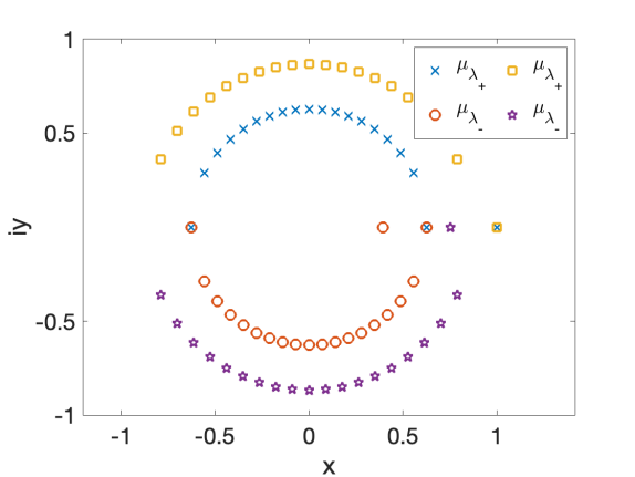
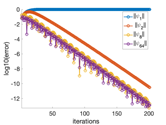
Second, for $\beta\in[\lambda_{2}^{2}/4,\lambda_{1}^{2}/4)$, except for $\mu_{\lambda_{1}}$ and $\widehat{\mu}_{\lambda_{1}}$ all the remaining $2n-2$ (complex) eigenvalues of $A_{\beta}$ (corresponding to the eigenvalues $\lambda_{2},\ldots,\lambda_{n}$ of $A$) have the same magnitude $\sqrt{\beta}$ according to (2.11). However, as the corresponding eigenvalues $\lambda_{j}$ of $A$ with $|\lambda_{j}|<|\lambda_{2}|$ decrease in magnitude, the argument $\theta$ in (2.11) increases. This causes oscillatory convergence at an increasing rate of oscillation for the subdominant modes. This is illustrated in figure 1: the left plot shows the ratio of eigenvalues $\mu_{\lambda_{\pm}}/\mu_{\lambda_{1}}$ of $A_{\beta}$ plotted on the complex plane for $\beta=9^{2}/4$ (inner circle) and $\beta=9.9^{2}/4$ (outer circle), where $A=\operatorname{diag}(10:-1:-9)$. The right plot shows the magnitude of the first, second, eighth and 64th eigenmodes of the power iteration algorithm 1.1 applied to the augmented matrix $A_{\beta}$ for $A=\operatorname{diag}(100:-1:1)$ with $\beta=99^{2}/4$. The plots agree with the above analysis: the modes all decay at the same rate, but the modes of $A_{\beta}$ corresponding to the eigenmodes of $A$ with smaller magnitude eigenvalues have larger imaginary parts, and their convergence is more oscillatory. The above analysis also shows that if $\beta\geq\lambda_{1}^{2}/4$, then all eigenvalues of $A_{\beta}$ have the same magnitude. Therefore, if $\beta\geq\lambda_{1}^{2}/4$, the augmented matrix $A_{\beta}$ does not satisfy assumption 1.2, and neither the power iteration applied to $A_{\beta}$, nor iteration 1.2 applied to $A$, will converge.

3 Dynamic momentum method

We would like to use the acceleration of the momentum algorithm 1.2, but without the a priori knowledge of $\lambda_{2}$. A method for determining an effective sequence of momentum parameters is presented in [22, algorithm 3], called the Best Heavy Ball method. This method however requires five matrix-vector multiplications per iteration, as compared to the single matrix-vector multiplication per iteration required by the standard power iteration algorithm 1.1 or the momentum accelerated power iteration [22] presented here as algorithm 1.2. This is improved upon in the DMPower algorithm of [21] which uses inexact deflation [23, chapter 4] in a preliminary iteration to approximate $\lambda_{2}$. However, the method is sensitive to the approximation of $\lambda_{2}$, and ensuring the approximation is good enough again requires a priori knowledge of the spectrum. Additionally, the preliminary iteration is more computationally expensive, requiring 3 matrix-vector multiplications per iteration.

Our approach for approximating the momentum parameter $\beta=\lambda_{2}^{2}/4$ does not require any additional matrix-vector multiplication per iteration. We obtain an expression for $r_{k+1}$, as an approximation of $r=|\lambda_{2}/\lambda_{1}|$ from the detected residual convergence rate $\rho_{k}=d_{k+1}/d_{k}$ by inverting the optimal convergence rate (2.16) for $r$ in terms of $\rho$. This is justified in lemma 3.4. We then approximate $\lambda_{2}$ by $r_{k+1}$ multiplied by the (computed) Rayleigh quotient approximation to $\lambda_{1}$, which yields the approximated momentum parameter $\beta_{k}$. The resulting Dynamic Momentum algorithm is presented below.

Algorithm 3.3.

Dynamic momentum

Do two iterations of algorithm 1.1 $\triangleright$ $k=0,1$

Set $r_{2}=\min\{d_{2}/d_{1},1\}$

for $k\geq 2$ do $\triangleright$ $k\geq 2$

     Set $\beta_{k}=\nu_{k}^{2}r_{k}^{2}/4$

     Set $u_{k+1}=v_{k+1}-(\beta_{k}/h_{k})x_{k-1}$

     Set $h_{k+1}=\left\|{u_{k+1}}\right\|$ and $x_{k+1}=h_{k+1}^{-1}u_{k+1}$

     Set $v_{k+2}=Ax_{k+1}$, $\nu_{k+1}=(v_{k+2},x_{k+1})$ and $d_{k+1}=\left\|{v_{k+2}-\nu_{k+1}x_{k+1}}\right\|$

     Update $\rho_{k}=\min\{d_{k+1}/d_{k},1\}$ and $r_{k+1}=2\rho_{k}/(1+\rho_{k}^{2})$

     STOP if $\left\|{d_{k+1}}\right\|<$ tol

end for

Lemma 3.4 and remark 3.5 in the next section show that assigning $r_{k+1}$ by $r_{k+1}={2\rho_{k}}/(1+\rho_{k}^{2})$, obtained by inverting the asymptotic convergence rate (2.16) of the optimal parameter $\beta$, gives a stable approximation to $r$ and hence to $\beta$. In fact, the approximation becomes increasingly stable as $r$ gets closer to unity.

The next remark describes the role of the subdominant eigenmodes in the residual.

Remark 3.1.

The residual $d_{k}$ as given in algorithms 1.1, 1.2 and 3.3 is given by $d_{k}=\left\|{Ax_{k}-\nu_{k}x_{k}}\right\|$ where the Rayleigh quotient $\nu_{k}$ is given by $(Ax_{k},x_{k})$. Let $x_{k}=\sum_{l=1}^{n}\alpha_{l}^{(k)}\phi_{l}$ where $\{\phi_{l}\}_{l=1}^{n}$ is the eigenbasis of $A$. Then

$$d_{k}=\left\|{\sum_{l=1}^{n}(\lambda_{l}\alpha_{l}^{(k)}\phi_{l})-\sum_{l=1}^{n}(\nu_{k}\alpha_{l}^{(k)}\phi_{l})}\right\|=\left\|{\sum_{l=1}^{n}(\lambda_{l}-\nu_{k})\alpha_{l}^{(k)}\phi_{l}}\right\|.$$ (3.1)

The detected convergence rate $\rho_{k}$ is given by

$$\rho_{k}=\frac{d_{k+1}}{d_{k}}=\frac{\left\|{\sum_{l=1}^{n}(\lambda_{l}-\nu_{k+1})\alpha_{l}^{(k+1)}\phi_{l}}\right\|}{\left\|{\sum_{l=1}^{n}(\lambda_{l}-\nu_{k})\alpha_{l}^{(k)}\phi_{l}}\right\|}.$$ (3.2)

We will consider the preasymptotic regime to be that in which $\lambda_{1}-\nu_{k}$ is not negligible in comparison to the coefficients $\alpha_{l}^{(k)},~{}l>1$, which will be seen to deteriorate. In the asymptotic regime, we have $\nu_{k}\approx\lambda_{1}$ hence (3.2) reduces for practical purposes to

$$\rho_{k}\approx\frac{\left\|{\sum_{l=2}^{n}(\lambda_{l}-\nu_{k+1})\alpha_{l}^{(k+1)}\phi_{l}}\right\|}{\left\|{\sum_{l=2}^{n}(\lambda_{l}-\nu_{k})\alpha_{l}^{(k)}\phi_{l}}\right\|}.$$ (3.3)

In the usual analysis of the power iteration, coefficients $\alpha_{l}^{(k+1)}$ deteriorate like $\lambda_{l}/\lambda_{1}$ at each iteration as in (2.5), hence eventually (3.3) is dominated by the maximal such ratio $\lambda_{2}/\lambda_{1}$. In contrast, in the case of the augmented matrix $A_{\beta_{k}}$, for each of the eigenmodes with $\lambda^{2}/4<\beta_{k}$, each of the corresponding eigenvalues has the same magnitude; and, as shown in (2.11) increasing imaginary parts as corresponding eigenvalues of $A$ decrease. Hence it is not necessarily the case that the second eigenmode will dominate (3.3) through most of the iteration. The oscillation of the subdominant modes is the main reason we will see the sequence of convergence rates $\rho_{k}$ fluctuate in the dynamic algorithm.

However, the stability of $r_{k}$ with respect to $\rho_{k}$ shown in lemma 3.4 controls the oscillations in $r_{k}$ with respect to $\rho_{k}$, and substantially damps them in the case that $r=|\lambda_{2}/\lambda_{1}|$ is close to unity. In this case there is a more substantial relative gap between the convergence rate for the second eigenmode and the higher frequency modes, so long as some of the $\beta_{k}$ satisfy $\beta_{k}<\lambda_{2}^{2}/4$, which is generally the case. Then the second eigenmode does (eventually) tend to dominate the residual. A further discussion of the coefficients $\alpha_{l}^{(k)}$ will be given in remark 3.6, where it will be shown that $\alpha_{l}^{(k)}$ is controlled by the product of eigenvalues of the sequence of augmented matrices $A_{\beta_{k}}$ corresponding to $\lambda_{l}$ of $A$. The differences in convergence behavior between smaller and larger values of $r$ are highlighted in section 5.

The following subsection takes into account the nontrivial detail that the dynamic algorithm 3.3 differs from a standard power method in that a different augmented matrix $A_{\beta_{k}}$ is applied at each iteration.

3.1 Convergence theory

In Section 2.1, we interpret the convergence of the momentum method with constant $\beta$ as a power method applied to the augmented matrix $A_{\beta}$. However, this perspective no longer precisely holds for algorithm 3.3 as the parameter $\beta_{k}$ is subject to change at each step. Consequently, the corresponding augmented matrix $A_{\beta_{k}}$ changes at each step as well. This presents a significant challenge in the analysis of the dynamic momentum algorithm.

For ease of presentation, we next define some notation to be used throughout the remainder of this section. Let

$$A^{(0)}=\begin{pmatrix}A&0\\ I&0\end{pmatrix},\quad\text{ and }\quad A^{(j)}=A_{\beta_{j}}=\begin{pmatrix}A&-\beta_{j}I\\ I&0\end{pmatrix},~{}j\geq 1,$$

where $A^{(0)}$ is the augmented matrix with $\beta=0$. As in subsection 1.1, let $\{\phi_{l}\}_{l=1}^{n}$ be an eigenbasis of $A$, with corresponding eigenvalues $\{\lambda_{l}\}_{l=1}^{n}$. For each eigenpair $(\lambda_{l},\phi_{l})$ of $A$, denote $(\mu^{(j)}_{l},\psi^{(j)}_{l})$ the corresponding eigenpair of $A^{(j)}$ where $\mu_{l}^{(j)}$ is the eigenvalue with larger magnitude defined in (2.9)-(2.11). Then by (2.8)

$$\psi^{(j)}_{l}=\begin{pmatrix}\mu^{(j)}\phi_{l}\\ \phi_{l}\end{pmatrix},$$

for $j\geq 0$ with $\mu_{l}^{(0)}=\lambda_{l}$.

In the first technical lemma of this section we show the effect of applying a sequence of augmented matrices with changing parameter $\beta_{j}$ to each eigenmode of $A$.

Lemma 3.2.

Let $A$ satisfy assumption 1.1, let $(\lambda,\phi)$ be an eigenpair of $A$, and let $\mu^{(j)}$ be the corresponding eigenvalue of $A^{(j)}$, as in proposition 2.1. Let $\delta_{ik}=\mu^{(i)}-\mu^{(k)}$. Define ${\mathcal{P}}^{i}(\mu)$ to be a product of $i$ terms $\mu^{(k)}$, where $1\leq k\leq j$, and ${\mathcal{P}}^{i}(\delta)$ to be a product of $i$ terms $\delta_{kp}$, where $0\leq k,p\leq j$. Then

$$A^{(j)}\cdots A^{(0)}\begin{pmatrix}\phi\\ 0\end{pmatrix}=\left(\prod_{i=1}^{j}\mu^{(i)}+\sum_{k=1}^{j-1}\delta_{k-1,k}\prod_{i=1,i\neq k}^{j}\mu^{(i)}+\sum_{i=2}^{j-1}{\mathcal{P}}^{i}(\delta){\mathcal{P}}^{j-i}(\mu)\right)\begin{pmatrix}\mu^{(j)}\phi\\ \phi\end{pmatrix}$$

$$+\left(\delta_{j-1,j}\prod_{i=1}^{j-1}\mu^{(i)}+\sum_{i=2}^{j}{\mathcal{P}}^{i}(\delta){\mathcal{P}}^{j-i}(\mu)\right)\begin{pmatrix}\mu^{(0)}\phi\\ \phi\end{pmatrix}.$$ (3.4)

This lemma shows that applying the sequence of augmented matrices $A^{(j)}\cdots A^{(0)}$ to each eigenmode of $A$ yields a perturbation to multiplying the eigenmode of $A^{(j)}$ associated with eigenmode $\phi$ of $A$ by $\mu^{(1)}\mu^{(2)}\cdots\mu^{(j)}$. The higher-order in $\delta$ terms of (3.2) are given in a form that will be used in the next technical lemma. The ${\mathcal{P}}^{i}()$ notation is introduced to state the relevant result without keeping track of the specific factors in each product.

Proof.

The proof relies on two repeated calculations. First, for any $\alpha,\beta$

$$A_{\beta}\begin{pmatrix}\alpha\phi\\ 0\end{pmatrix}=\begin{pmatrix}A&-\beta I\\ I&0\end{pmatrix}\begin{pmatrix}\alpha\phi\\ 0\end{pmatrix}=\alpha\begin{pmatrix}\lambda\phi\\ \phi\end{pmatrix}=\alpha\begin{pmatrix}\mu^{(0)}\phi\\ \phi\end{pmatrix},$$ (3.5)

where $\mu^{(0)}:=\lambda$. Second,

$$A^{(k)}\begin{pmatrix}\mu^{(j)}\phi\\ \phi\end{pmatrix} =A^{(k)}\begin{pmatrix}\mu^{(k)}\phi\\ \phi\end{pmatrix}+A^{(k)}\begin{pmatrix}\delta_{jk}\phi\\ 0\end{pmatrix}=\mu^{(k)}\begin{pmatrix}\mu^{(k)}\phi\\ \phi\end{pmatrix}+A^{(k)}\begin{pmatrix}\delta_{jk}\phi\\ 0\end{pmatrix}$$

$$=\mu^{(k)}\begin{pmatrix}\mu^{(k)}\phi\\ \phi\end{pmatrix}+\delta_{jk}\begin{pmatrix}\mu^{(0)}\phi\\ \phi\end{pmatrix},$$ (3.6)

where the last term in (3.1) is the result of (3.5).

Starting with (3.5), and proceeding to apply (3.1) we have

$$A^{(0)} \begin{pmatrix}\phi\\ 0\end{pmatrix}=\begin{pmatrix}\mu^{(0)}\phi\\ \phi\end{pmatrix},$$ (3.7)

$$A^{(1)}A^{(0)} \begin{pmatrix}\phi\\ 0\end{pmatrix}=\mu^{(1)}\begin{pmatrix}\mu^{(1)}\phi\\ \phi\end{pmatrix}+\delta_{01}\begin{pmatrix}\mu^{(0)}\phi\\ \phi\end{pmatrix},$$ (3.8)

$$A^{(2)}A^{(1)}A^{(0)} \begin{pmatrix}\phi\\ 0\end{pmatrix}=\mu^{(2)}\mu^{(1)}\begin{pmatrix}\mu^{(2)}\phi\\ \phi\end{pmatrix}+\delta_{12}\mu^{(1)}\begin{pmatrix}\mu^{(0)}\phi\\ \phi\end{pmatrix}+\delta_{01}\mu^{(2)}\begin{pmatrix}\mu^{(2)}\phi\\ \phi\end{pmatrix}+\delta_{02}\delta_{01}\begin{pmatrix}\mu^{(0)}\phi\\ \phi\end{pmatrix}$$

$$=\left(\mu^{(2)}\mu^{(1)}+\delta_{01}\mu^{(2)}\right)\begin{pmatrix}\mu^{(2)}\phi\\ \phi\end{pmatrix}+\left(\delta_{12}\mu^{(1)}+{\mathcal{P}}^{2}(\delta)\right)\begin{pmatrix}\mu^{(0)}\phi\\ \phi\end{pmatrix}.$$ (3.9)

One more iteration reveals the form of the higher order terms.

$$A^{(3)}A^{(2)}A^{(1)}A^{(0)}\begin{pmatrix}\phi\\ 0\end{pmatrix} =\left(\mu^{(2)}\mu^{(1)}+\delta_{01}\mu^{(2)}\right)\left(\mu^{(3)}\begin{pmatrix}\mu^{(3)}\phi\\ \phi\end{pmatrix}+\delta_{23}\begin{pmatrix}\mu^{(0)}\phi\\ \phi\end{pmatrix}\right)$$

$$+\left(\delta_{12}\mu^{(1)}+{\mathcal{P}}^{2}(\delta)\right)\left(\mu^{(3)}\begin{pmatrix}\mu^{(3)}\phi\\ \phi\end{pmatrix}+\delta_{03}\begin{pmatrix}\mu^{(0)}\phi\\ \phi\end{pmatrix}\right)$$

$$=\left(\mu^{(3)}\mu^{(2)}\mu^{(1)}+\delta_{01}\mu^{(3)}\mu^{(2)}+\delta_{12}\mu^{(3)}\mu^{(1)}+{\mathcal{P}}^{2}(\delta){\mathcal{P}}(\mu)\right)\begin{pmatrix}\mu^{(3)}\phi\\ \phi\end{pmatrix}$$

$$+\left(\delta_{23}\mu^{(2)}\mu^{(1)}+{\mathcal{P}}^{2}(\delta){\mathcal{P}}(\mu)+{\mathcal{P}}^{3}(\delta)\right)\begin{pmatrix}\mu^{(0)}\phi\\ \phi\end{pmatrix}.$$ (3.10)

Now we may proceed inductively. Suppose

$$\Phi^{(j)}:=A^{(j)}\cdots A^{(0)}\begin{pmatrix}\phi\\ 0\end{pmatrix}=\left(\prod_{i=1}^{j}\mu^{(i)}+\sum_{k=1}^{j-1}\delta_{k-1,k}\prod_{i=1,i\neq k}^{j}\mu^{(i)}+\sum_{i=2}^{j-1}{\mathcal{P}}^{i}(\delta){\mathcal{P}}^{j-i}(\mu)\right)\begin{pmatrix}\mu^{(j)}\phi\\ \phi\end{pmatrix}$$

$$+\left(\delta_{j-1,j}\prod_{i=1}^{j-1}\mu^{(i)}+\sum_{i=2}^{j}{\mathcal{P}}^{i}(\delta){\mathcal{P}}^{j-i}(\mu)\right)\begin{pmatrix}\mu^{(0)}\phi\\ \phi\end{pmatrix}.$$ (3.11)

We will show

$$\Phi^{(j+1)} =\left(\prod_{i=1}^{j+1}\mu^{(i)}+\sum_{k=1}^{j}\delta_{k-1,k}\prod_{i=1,i\neq k}^{j+1}\mu^{(i)}+\sum_{i=2}^{j}{\mathcal{P}}^{i}(\delta){\mathcal{P}}^{j+1-i}(\mu)\right)\begin{pmatrix}\mu^{(j+1)}\phi\\ \phi\end{pmatrix}$$

$$+\left(\delta_{j,j+1}\prod_{i=1}^{j}\mu^{(i)}+\sum_{i=2}^{j+1}{\mathcal{P}}^{i}(\delta){\mathcal{P}}^{j+1-i}\mu)\right)\begin{pmatrix}\mu^{(0)}\phi\\ \phi\end{pmatrix}.$$ (3.12)

The base step of the induction is satisfied by (3.1). For the inductive step, applying (3.1) to $A^{(j+1)}\Phi^{(j)}$ yields

$$A^{(j+1)}\Phi^{(j)} =\mu^{(j+1)}\left\{\left(\prod_{i=1}^{j}\mu^{(i)}+\sum_{k=1}^{j-1}\delta_{k-1,k}\prod_{i=1,i\neq k}^{j}\mu^{(i)}+\sum_{i=2}^{j-1}{\mathcal{P}}^{i}(\delta){\mathcal{P}}^{j-i}(\mu)\right)\right.$$

$$+\left.\left(\delta_{j-1,j}\prod_{i=1}^{j-1}\mu^{(i)}+\sum_{i=2}^{j}{\mathcal{P}}^{i}(\delta){\mathcal{P}}^{j-i}(\mu)\right)\right\}\begin{pmatrix}\mu^{(j+1)}\phi\\ \phi\end{pmatrix}$$

$$+\left\{\delta_{j,j+1}\left(\prod_{i=1}^{j}\mu^{(i)}+\sum_{k=1}^{j-1}\delta_{k-1,k}\prod_{i=1,i\neq k}^{j}\mu^{(i)}+\sum_{i=2}^{j-1}{\mathcal{P}}^{i}(\delta){\mathcal{P}}^{j-i}(\mu)\right)\right.$$

$$\left.+\delta_{0,j+1}\left(\delta_{j-1,j}\prod_{i=1}^{j-1}\mu^{(i)}+\sum_{i=2}^{j}{\mathcal{P}}^{i}(\delta){\mathcal{P}}^{j-i}(\mu)\right)\right\}\begin{pmatrix}\mu^{(0)}\phi\\ \phi\end{pmatrix},$$

which after multiplying though and combining the ${\mathcal{P}}(\cdot)$ terms of like order agrees with (3.1). ∎

This establishes the result (3.2). The next step in the proof is to generalize the first component of the initial vector used in lemma 3.2 from a single eigenmode of $A$ to a linear combination of eigenmodes of $A$, to arrive an an estimate analogous to (2.5).

Lemma 3.3.

Let $A$ satisfy assumption 1.1. Let $\delta_{l,i,k}=\mu_{l}^{(i)}-\mu_{l}^{(k)}$. As in lemma 3.2, define ${\mathcal{P}}^{i}(\mu_{l})$ to be a product of $i$ terms $\mu_{l}^{(k)}$, where $1\leq k\leq j$, and ${\mathcal{P}}^{i}(\delta_{l})$ to be a product of $i$ terms $\delta_{l,k,p}$, where $0\leq k,p\leq j$. Let $u_{0}=\sum_{l=1}^{n}a_{l}\phi_{l}$, a linear combination of the eigenvectors of $A$. Then it holds that the product $A^{(j)}A^{(j-1)}\cdots A^{(0)}\begin{pmatrix}u_{0}\\ 0\end{pmatrix}$ satisfies

$$A^{(j)}A^{(j-1)}\cdots A^{(0)}\begin{pmatrix}u_{0}\\ 0\end{pmatrix} =a_{1}\left(\prod_{i=1}^{j}\mu_{1}^{(i)}\right)\left\{\psi_{1}^{(j)}+\sum_{l=2}^{n}\frac{a_{l}}{a_{1}}\left(\prod_{i=1}^{j}\frac{\mu_{l}^{(i)}}{\mu_{1}^{(i)}}\right)\psi_{l}^{(j)}\right\}$$

$$+\sum_{i=1}^{j-1}a_{1}{\mathcal{P}}^{j-i}(\mu_{1})\left\{\psi_{1}^{(j)}{\mathcal{P}}^{i}(\delta_{1})+\sum_{l=2}^{n}\frac{a_{l}}{a_{1}}{\mathcal{P}}^{i}(\delta_{l}){\mathcal{P}}^{j-i}\left(\frac{\mu_{l}}{\mu_{1}}\right)\psi_{l}^{(j)}\right\}$$

$$+\sum_{i=1}^{j}a_{1}{\mathcal{P}}^{j-i}(\mu_{1})\left\{\psi_{1}^{(0)}{\mathcal{P}}^{i}(\delta_{1})+\sum_{l=2}^{n}\frac{a_{l}}{a_{1}}{\mathcal{P}}^{i}(\delta_{l}){\mathcal{P}}^{j-i}\left(\frac{\mu_{l}}{\mu_{1}}\right)\psi_{l}^{(0)}\right\}.$$ (3.13)

Supposing additionally that $\mu_{1}^{(i)}>\delta_{l,k,p}$ for any $i,k,p=1,\ldots,j$, and $l\geq 2$, then as $j$ increases, the product $A^{(j)}A^{(j-1)}\cdots A^{(0)}u_{0}$ aligns to a linear combination of $\psi_{1}^{(j)}$ and $\psi_{1}^{(0)}.$

The proof shows additional detail on the ${\mathcal{O}}(\delta)$ terms, as revealed in lemma 3.2. This lemma shows that the product of the sequence of matrices $A^{(j)}\ldots A^{(0)}$ applied to a vector with a general first component, $u_{0}\in\mathbb{R}^{n}$ and null second component $0\in\mathbb{R}^{n}$ aligns with a vector whose first component is the dominant eigenvector $\phi_{1}$ of $A$. It will be shown in theorem 3.1 that the convergence is similar to the power method with $(\lambda_{l}/\lambda_{1})^{j}$ as in (2.5) replaced by the product $(\mu_{l}^{(1)}\cdots\mu_{l}^{(j)})/(\mu_{1}^{(1)}\cdots\mu_{1}^{(j)})$. The appreciable difference in the convergence is from the contribution of the $\delta$-scaled terms which are in the directions of the eigenvectors $\psi_{l}^{(j)}$ and $\psi_{l}^{(0)}$, with $l=1,\ldots,n$. As we will see in theorem 3.1 and remark 3.6, these terms will not interfere with convergence or the asymptotically expected rate, due to the stability of the parameters $\beta_{i}$, as shown in lemma 3.4.

Proof.

First by applying linearity and (3.2) we have

$$A^{(j)}\cdots A^{(0)}\begin{pmatrix}u_{0}\\ 0\end{pmatrix} =\sum_{l=1}^{n}a_{l}A^{(j)}\cdots A^{(0)}\begin{pmatrix}\phi_{l}\\ 0\end{pmatrix}$$

$$=\sum_{l=1}^{n}a_{l}\left(\prod_{i=1}^{j}\mu_{l}^{(i)}+\sum_{k=1}^{j-1}\delta_{l,k-1,k}\prod_{i=1,i\neq k}^{j}\mu_{l}^{(i)}+\sum_{i=2}^{j-1}{\mathcal{P}}^{i}(\delta_{l}){\mathcal{P}}^{j-i}(\mu_{l})\right)\begin{pmatrix}\mu_{l}^{(j)}\phi_{l}\\ \phi_{l}\end{pmatrix}$$

$$+\sum_{l=1}^{n}a_{l}\left(\delta_{l,j-1,j}\prod_{i=1}^{j-1}\mu_{l}^{(i)}+\sum_{i=2}^{j}{\mathcal{P}}^{i}(\delta_{l}){\mathcal{P}}^{j-i}(\mu_{l})\right)\begin{pmatrix}\mu_{l}^{(0)}\phi_{l}\\ \phi_{l}\end{pmatrix}.$$ (3.14)

Now we will examine each term of (3.1).

We rewrite the first term in the right hand side of (3.1) as

$$\sum_{l=1}^{n}a_{l}\left(\prod_{i=1}^{j}\mu_{l}^{(i)}\right)\psi_{l}^{(j)}=a_{1}\left(\prod_{i=1}^{j}\mu_{1}^{(i)}\right)\left\{\psi_{1}^{(j)}+\sum_{l=2}^{n}\frac{a_{l}}{a_{1}}\left(\prod_{i=1}^{j}\frac{\mu_{l}^{(i)}}{\mu_{1}^{(i)}}\right)\psi_{l}^{(j)}\right\}.$$ (3.15)

This is similar to (2.5) and displays convergence to $\psi_{1}$ so long as the other terms do not interfere. The second term in the right hand side of (3.1) can be written as

$$\sum_{l=1}^{n}a_{l}\sum_{k=1}^{j-1}\delta_{l,k-1,k}\left(\prod_{i=1,i\neq k}^{j}\mu_{l}^{(i)}\right)\psi_{l}^{(j)}$$

$$= \sum_{k=1}^{j-1}a_{1}\left(\prod_{i=1,i\neq k}^{j}\mu_{1}^{i}\right)\left\{\delta_{1,k-1,k}\psi_{1}^{(j)}+\sum_{l=2}^{n}\frac{a_{l}}{a_{1}}\delta_{l,k-1,k}\left(\prod_{i=1,i\neq k}^{j}\frac{\mu_{l}^{(i)}}{\mu_{1}^{(i)}}\right)\psi_{l}^{(j)}\right\},$$ (3.16)

which is an ${\mathcal{O}}(\delta)$ term where the factors of $\mu^{(i)}_{l}/\mu^{(i)}_{1}$ multiplying the subdominant eigenmodes are one power lower than in the dominant term (3.15). The higher order terms multiplying the eigenvectors of $A^{(j)}$ are

$$\sum_{l=1}^{n}a_{l}\sum_{i=2}^{j-1}{\mathcal{P}}^{i}(\delta_{l}){\mathcal{P}}^{j-i}(\mu_{l})\psi_{l}^{(j)}=\sum_{i=2}^{j-1}a_{1}{\mathcal{P}}^{j-i}(\mu_{1})\left\{\psi_{1}^{(j)}{\mathcal{P}}^{i}(\delta_{1})+\sum_{l=2}^{n}\frac{a_{l}}{a_{1}}{\mathcal{P}}^{i}(\delta_{l}){\mathcal{P}}^{j-i}\left(\frac{\mu_{l}}{\mu_{1}}\right)\psi_{l}^{(j)}\right\}.$$ (3.17)

Next, we look at the terms of (3.1) multiplying the eigenvectors $\psi_{0}^{(0)}$ of $A^{(0)}$. The lowest order term is ${\mathcal{O}}(\delta)$ and is given by

$$\sum_{l=1}^{n}a_{l}\delta_{l,j-1,j}\left(\prod_{i=1}^{j-1}\mu_{l}^{(i)}\right)=a_{1}\left(\prod_{i=1}^{j-1}\mu_{1}^{(i)}\right)\left\{\delta_{1,j-1,j}\psi_{1}^{(0)}+\frac{a_{l}}{a_{1}}\delta_{l,j-1,j}\left(\prod_{i=1}^{j-1}\frac{\mu_{l}^{(i)}}{\mu_{1}^{(i)}}\right)\psi_{l}^{(0)}\right\}.$$ (3.18)

Last we have the higher order terms

$$\sum_{l=1}^{n}a_{l}\left(\sum_{i=2}^{j}{\mathcal{P}}^{i}(\delta_{l}){\mathcal{P}}^{j-i}(\mu_{l})\right)\psi_{l}^{(0)}=\sum_{i=2}^{j}a_{1}{\mathcal{P}}^{j-i}(\mu_{1})\left\{\psi_{1}^{(0)}{\mathcal{P}}^{i}(\delta_{1})+\sum_{l=1}^{n}\frac{a_{l}}{a_{1}}{\mathcal{P}}^{i}(\delta_{l}){\mathcal{P}}^{j-i}\left(\frac{\mu_{l}}{\mu_{1}}\right)\psi_{l}^{(0)}\right\}.$$ (3.19)

Sweeping the results of the more detailed (3.1) into (3.17), and likewise (3.18) into (3.19) yields the result (3.3). Finally, the alignment of the product (3.3) to a combination of $\psi_{1}^{(j)}$ and $\psi_{1}^{(0)}$ follows from noting each ratio $(\mu^{(i)}_{l}/\mu^{(i)}_{1})<1$ and applying the hypothesis $\mu_{1}^{(i)}>\delta_{l,k,p}$ for any $i,k,p=1,\ldots,j$, and $l\geq 2$. ∎

The next lemma shows that if $\rho_{k}$ is an $\varepsilon$ perturbation of $\rho=|\mu_{2}/\mu_{1}|$, then $r_{k+1}$ is an $\widehat{\varepsilon}$ perturbation of $r$, where $\widehat{\varepsilon}<2\varepsilon$ for $\rho\in(0,1)$, and $\widehat{\varepsilon}\rightarrow 0$ as $\rho\rightarrow 1$. This means the smaller the spectral gap in $A$, the more stable the dynamic momentum method becomes.

Lemma 3.4.

Let $\rho\in(0,1)$ and consider $\varepsilon$ small enough so that $(2\rho\varepsilon+\varepsilon^{2})/(1+\rho^{2})<1$. Let $\rho_{k}=\rho+\varepsilon$ and define $r_{k+1}=2\rho_{k}/(1+\rho_{k}^{2})$, as in algorithm 3.3. Then

$$r_{k+1}=r+\widehat{\varepsilon}+{\mathcal{O}}(\varepsilon^{2})~{}\text{ with }~{}\widehat{\varepsilon}=\varepsilon\frac{2(1-\rho^{2})}{(1+\rho^{2})^{2}}.$$ (3.20)

The condition $(2\rho\varepsilon+\varepsilon^{2})/(1+\rho^{2})<1$ is satisfied for $\rho\in(0,1)$ by $\varepsilon<0.71$.

Proof.

For $r=|\lambda_{2}/\lambda_{1}|$ the asymptotic convergence rate of iteration (1.2) is $\rho=r(1+\sqrt{1-r^{2}})^{-1}$, as given by (2.16), when $\beta=\lambda_{2}^{2}/4$. Inverting this expression for $r$ in terms of $\rho$ yields

$$r=\frac{2\rho}{1+\rho^{2}}.$$ (3.21)

Suppose the detected convergence rate $\rho_{k}=d_{k+1}/d_{k}$ is an $\epsilon$ perturbation of $\rho$, meaning $\rho_{k}=\rho+\varepsilon$. Expanding $r_{k+1}=2\rho_{k}/(1+\rho_{k}^{2})$ in $\varepsilon$ yields

$$r_{k+1} =\frac{2\rho}{1+(\rho+\varepsilon)^{2}}+\frac{2\varepsilon}{1+(\rho+\varepsilon)^{2}}$$

$$=\frac{2\rho}{1+\rho^{2}}\left(\frac{1}{1+\frac{2\rho\varepsilon+\varepsilon^{2}}{1+\rho^{2}}}\right)+\frac{2\varepsilon}{1+\rho^{2}}\left(\frac{1}{1+\frac{2\rho\varepsilon+\varepsilon^{2}}{1+\rho^{2}}}\right)$$

$$=\frac{2\rho}{1+\rho^{2}}\left(1-\frac{2\rho\varepsilon+\varepsilon^{2}}{1+\rho^{2}}+{\mathcal{O}}(\varepsilon^{2})\right)+\frac{2\varepsilon}{1+\rho^{2}}+{\mathcal{O}}(\varepsilon^{2}).$$ (3.22)

Applying (3.21) to (3.1) yields

$$r_{k+1}=r\left(1+\varepsilon\left(\frac{1}{\rho}-r\right)\right)+{\mathcal{O}}(\varepsilon^{2})=r+\widehat{\varepsilon}+{\mathcal{O}}(\varepsilon^{2}),~{}\text{ where }~{}\widehat{\varepsilon}=r\varepsilon\left(\frac{1}{\rho}-r\right).$$ (3.23)

Applying (3.21) to (3.23) yields the result (3.20), by which $\widehat{\varepsilon}<2\varepsilon$ for $\rho\in(0,1)$, and $\widehat{\varepsilon}<\varepsilon$ for $\rho\in(0.486,1)$, or $r\in(0.786,1)$. Moreover as $r$ getting closer to unity, the approximation becomes more stable, with $\widehat{\varepsilon}<0.161\cdot\varepsilon$ for $r\in(0.99,1)$ and $\widehat{\varepsilon}<0.0468\cdot\varepsilon$ for $r\in(0.999,1)$. ∎

The stability of $\beta_{k}=(r_{k}\nu_{k})^{2}/4$ in algorithm 3.3 is inherited directly from the stability of $r_{k}$, once $\nu_{k}$ sufficiently converges to $\lambda_{1}$.

Remark 3.5.

Another way to view how close $\beta_{k}$ is to $\beta=\beta_{opt}=\lambda_{2}^{2}/4$ with respect to $r_{k}$ and $\rho_{k}$ viewed as perturbations of $r$ and $\rho$ is to consider $\rho_{k}$ written as

$$\rho_{k}=\frac{r\sqrt{1+\varepsilon/r^{2}}}{1+\sqrt{1-r^{2}(1+\varepsilon/r^{2})}},$$

for some $\varepsilon$ with $-r^{2}<\varepsilon<1-r^{2}$. Applying $r_{k+1}=2\rho_{k}/(1+\rho_{k}^{2})$ we then have $r_{k+1}=r\sqrt{1+\varepsilon/r^{2}},$ by which $\beta_{k+1}=r^{2}(1+\varepsilon/r^{2})\nu_{k+1}^{2}/4$. For $\nu_{k+1}\approx\lambda_{1}$ this yields

$$\beta_{k+1}\approx\frac{\lambda_{2}^{2}}{4}+\varepsilon\frac{\lambda_{1}^{2}}{4},$$

which shows how perturbations $r_{k}$ with respect to $r$ result in perturbations to $\beta_{k}$ with respect to $\beta$.

Now we can summarize the results of this section in a convergence theorem.

Theorem 3.1.

Let $A$ satisfy assumption 1.1. Let $\delta_{l,i,k}=\mu_{l}^{(i)}-\mu_{l}^{(k)}$, and let $u_{0}=\sum_{l=1}^{n}a_{j}\phi_{j}$, a linear combination of the eigenvectors of $A$. Assume $\beta_{k}<\lambda_{1}^{2}/4$ for all $k$. Then (3.3) holds and algorithm 3.3 converges to the dominant eigenpair.

Here we proceed by assuming generically that none of the $\beta_{k}$ take a value of exactly equal to $\lambda^{2}/4$ for any eigenvalue $\lambda$ of $A$. This is a reasonable assumption due both to floating point arithmetic, and that as shown in lemma 3.4, the $\beta_{k}$ only converge to $\lambda_{2}^{2}/4$ as $r\rightarrow 1$, and we are always in the circumstance that $r<1$.

Proof.

We will start by developing bounds on the $\mu_{l}^{(i)}$ and the $\delta_{l,i,k}$, and in the process will verify the final hypothesis of lemma 3.3 by verifying $|\delta_{l,i,k}|\leq\max\{|\mu_{l}^{(i)}|,|\mu_{l}^{(k)}|\}$. We will also see that $\delta_{l,i,k}\rightarrow 0$ as $\beta_{i}-\beta_{k}\rightarrow 0$ for each $\lambda_{l}$. Consider $\lambda=\lambda_{l}\neq 0$. There are three cases we need to consider. Without loss of generality, suppose $\beta_{i}\geq\beta_{k}$.

1. If $\lambda^{2}/4\geq\beta_{i}$ then $\mu_{l}^{(i)}$ and $\mu_{l}^{(k)}$ are given by (2.9), and $|\mu_{l}^{(i)}|\in[|\lambda|/2,|\lambda|]$ for $l=2,\ldots,n$. Since we have $\beta<\lambda_{1}^{2}/4$ we have $|\mu_{1}^{(i)}|\in(|\lambda_{1}|/2,|\lambda_{1}|]$. To bound $\delta_{l,i,k}$ we have

   $$|\mu_{l}^{(i)}-\mu_{l}^{(k)}|=\frac{|\lambda|}{2}\left|\sqrt{1-4\beta_{i}/\lambda^{2}}-\sqrt{1-4\beta_{k}/\lambda^{2}}\right|<\frac{|\lambda|}{2}\leq|\mu_{l}^{(i)}|<|\mu_{l}^{(k)}|.$$ (3.24)

   It is clear from continuity and (3.24) that $\delta_{l,i,k}\rightarrow 0$ as $\beta_{i}-\beta_{k}\rightarrow 0$. We can also expand to first order to see how, yielding $|\delta_{l,i,k}|=|(\beta_{i}-\beta_{k})+\ldots|$.

2. If $\lambda^{2}/4\leq\beta_{i},\beta_{k}<\lambda_{1}^{2}/4$ then $\mu_{l}^{(i)}$ and $\mu_{l}^{(k)}$ are given by (2.11), and we have $|\mu_{l}^{(i)}|=\sqrt{\beta_{i}}$. In this case $\delta_{l,i,k}$ satisfies

   $$|\mu_{l}^{(i)}-\mu_{l}^{(k)}|=\left|\sqrt{\beta_{i}}\sqrt{1-\lambda^{2}/(4\beta_{i})}-\sqrt{\beta_{k}}\sqrt{1-\lambda^{2}/(4\beta_{k})}\right|\leq\sqrt{\beta_{i}}=|\mu_{l}^{(i)}|.$$ (3.25)

   From continuity and (3.25) it is clear that $\delta_{l,i,k}\rightarrow 0$ as $\beta_{k}-\beta_{i}\rightarrow 0$. Expanding (3.25) to first order to see how, yields $|\mu_{l}^{(i)}-\mu_{l}^{(k)}|=|(\sqrt{\beta_{i}}-\sqrt{\beta_{k}})(1-\lambda^{2}/8)+\ldots|$.

3. If $\beta_{k}\leq\lambda^{2}/4\leq\beta_{i}$, then we have

   $$\mu_{l}^{(i)}-\mu_{l}^{(k)}=\frac{\lambda}{2}+\frac{1}{2}\sqrt{\lambda^{2}-4\beta_{i}}-\left(\frac{\lambda}{2}+\frac{1}{2}\sqrt{\lambda^{2}-4\beta_{k}}\right)=\frac{i}{2}\sqrt{4\beta_{i}-\lambda^{2}}-\frac{1}{2}\sqrt{\lambda^{2}-4\beta_{k}},$$

   by which $|\mu_{l}^{(i)}-\mu_{l}^{(k)}|=\sqrt{\beta_{i}-\beta_{k}}\leq\sqrt{\beta_{i}}=|\mu_{l}^{(i)}|$.

Combining with the above results, we have $|\delta_{l,k,p}|\leq\max\{|\mu_{l}^{(k)}|,|\mu_{l}^{(p)}|\}$, for any $l,k,p=1,\ldots,j$.

We now have by lemma 3.3 that as $j$ increases, the product $A^{(j)}A^{(j-1)}\cdots A^{(0)}\begin{pmatrix}u_{0}\\ 0\end{pmatrix}$ aligns with a linear combination of $\psi_{1}^{(j)}$ and $\psi_{1}^{(0)}$. As in subsection 2.1, we now analyze the convergence of algorithm  3.3 by the convergence of

$$\begin{pmatrix}x_{j+1}\\ y_{j+1}\end{pmatrix}=\frac{1}{h_{j+1}}\begin{pmatrix}u_{j+1}\\ z_{j+1}\end{pmatrix}=\frac{1}{h_{j+1}}\left(\prod_{i=0}^{j}h_{i}^{-1}\right)A^{(j)}A^{(j-1)}\cdots A^{(0)}\begin{pmatrix}u_{0}\\ 0\end{pmatrix},$$ (3.26)

where $h_{j}=\left\|{u_{j}}\right\|$. Applying (3.3) to (3.26), we have

$$\begin{pmatrix}u_{j+1}\\ z_{j+1}\end{pmatrix} =\frac{a_{1}}{h_{0}}\left(\prod_{i=1}^{j}\frac{\mu_{1}^{(i)}}{h_{i}}\right)\left\{\psi_{1}^{(j)}+\sum_{l=2}^{n}\frac{a_{l}}{a_{1}}\left(\prod_{i=1}^{j}\frac{\mu_{l}^{(i)}}{\mu_{1}^{(i)}}\right)\psi_{l}^{(j)}\right\}$$

$$+\left(\prod_{i=0}^{j}\frac{1}{h_{i}}\right)\sum_{i=1}^{j-1}a_{1}{\mathcal{P}}^{j-i}(\mu_{1})\left\{\psi_{1}^{(j)}{\mathcal{P}}^{i}(\delta_{1})+\sum_{l=2}^{n}\frac{a_{l}}{a_{1}}{\mathcal{P}}^{i}(\delta_{l}){\mathcal{P}}^{j-i}\left(\frac{\mu_{l}}{\mu_{1}}\right)\psi_{l}^{(j)}\right\}$$

$$+\left(\prod_{i=0}^{j}\frac{1}{h_{i}}\right)\sum_{i=1}^{j}a_{1}{\mathcal{P}}^{j-i}(\mu_{1})\left\{\psi_{1}^{(0)}{\mathcal{P}}^{i}(\delta_{1})+\sum_{l=2}^{n}\frac{a_{l}}{a_{1}}{\mathcal{P}}^{i}(\delta_{l}){\mathcal{P}}^{j-i}\left(\frac{\mu_{l}}{\mu_{1}}\right)\psi_{l}^{(0)}\right\}.$$ (3.27)

Distributing through the normalization factors in (3.1) yields

$$\begin{pmatrix}u_{j+1}\\ z_{j+1}\end{pmatrix} =\frac{a_{1}}{h_{0}}\left(\prod_{i=1}^{j}\frac{\mu_{1}^{(i)}}{h_{i}}\right)\left\{\psi_{1}^{(j)}+\sum_{l=2}^{n}\frac{a_{l}}{a_{1}}\left(\prod_{i=1}^{j}\frac{\mu_{l}^{(i)}}{\mu_{1}^{(i)}}\right)\psi_{l}^{(j)}\right\}$$

$$+\sum_{i=1}^{j-1}\frac{a_{1}}{h_{0}}\left(\frac{{\mathcal{P}}^{j-i}(\mu_{1})}{\prod_{k=1}^{j-i}h_{k}}\right)\left\{\psi_{1}^{(j)}{\mathcal{P}}^{i}(\delta_{1})+\sum_{l=2}^{n}\frac{a_{l}}{a_{1}}\left(\frac{{\mathcal{P}}^{i}(\delta_{l})}{\prod_{k=j-i+1}^{j}h_{k}}\right){\mathcal{P}}^{j-i}\left(\frac{\mu_{l}}{\mu_{1}}\right)\psi_{l}^{(j)}\right\}$$

$$+\sum_{i=1}^{j}\frac{a_{1}}{h_{0}}\left(\frac{{\mathcal{P}}^{j-i}(\mu_{1})}{\prod_{k=1}^{j-i}h_{k}}\right)\left\{\psi_{1}^{(0)}{\mathcal{P}}^{i}(\delta_{1})+\sum_{l=2}^{n}\frac{a_{l}}{a_{1}}\left(\frac{{\mathcal{P}}^{i}(\delta_{l})}{\prod_{k=j-i+1}^{j}h_{k}}\right){\mathcal{P}}^{j-i}\left(\frac{\mu_{l}}{\mu_{1}}\right)\psi_{l}^{(0)}\right\}.$$ (3.28)

By the arguments above, $\begin{pmatrix}u_{j+1}\\ z_{j+1}\end{pmatrix}$ aligns with a linear combination of $\psi_{1}^{(j)}$ and $\psi_{1}^{(0)}$, both of which have first components in the direction of $\phi_{1}$. This further shows that the Rayleigh quotient $\nu_{k}=(Ax_{k},x_{k})\rightarrow\lambda_{1}$, by which the residual (3.1) converges to zero. ∎

We conclude this section with a heuristic discussion of the coefficients of each eigenmode that appear in the residual, as per remark 3.1.

Remark 3.6.

By theorem 3.1, the Rayleigh quotient $\nu_{k}$ converges to $\lambda_{1}$. As in remark 3.1, we consider the asymptotic regime where $\nu_{k}\approx\lambda_{1}$, so that the ratio between consecutive residuals $\rho_{k}$ is well approximated by

$$\rho_{j}\approx\frac{\left\|{\sum_{l=2}^{n}(\lambda_{l}-\nu_{j+1})\alpha_{l}^{(j+1)}\phi_{l}}\right\|}{\left\|{\sum_{l=2}^{n}(\lambda_{l}-\nu_{j})\alpha_{l}^{(j)}\phi_{l}}\right\|}.$$ (3.29)

From (3.29), and the definition of the eigenvectors of the augmented matrix in (2.8), the coefficients $\alpha_{l}^{(j+1)}$, $l\geq 2$ are given by

$$\alpha_{l}^{(j+1)}=\frac{a_{l}}{\prod_{i=0}^{j+1}h_{i}}\left\{\mu_{l}^{(j)}\left(\prod_{i=1}^{j}\mu_{l}^{(i)}\right)+\sum_{i=1}^{j-1}(\mu_{l}^{(j)}+1){\mathcal{P}}^{j-i}(\mu_{l}){\mathcal{P}}^{i}(\delta_{l})+{\mathcal{P}}^{j}(\delta_{l})\right\}.$$ (3.30)

We next make the argument that the first term inside the brackets in (3.30) dominates the others.

From theorem 3.1, each $\delta_{l,i,k}$ satisfies $|\delta_{l,i,k}|\leq\max\{\mu_{l}^{(i)},\mu_{l}^{(k)}\}$. Referring to the proof of lemma 3.2, each of the factors of $\delta_{l,i,k}$ have either the form $\delta_{l,p-1,p}$ or $\delta_{l,0,p}$, where $p$ ranges from $1$ to $j+1$. As per the discussion in theorem 3.1, the terms of the form $\delta_{l,p-1,p}$ go to zero as the $\beta_{k}\rightarrow\beta=\lambda_{2}^{2}/4$. By lemma 3.4, considering the detected convergence rate $\rho_{k}$ as a perturbation of the theoretically optimal rate $\rho$, the computed approximation $r_{k+1}$ to $r=|\lambda_{2}/\lambda_{1}|$ is restricted to a tighter interval about $r$ when $r$ is closer to one. By this argument, and remark 3.5, $\beta_{k+1}$ is restricted to a small interval around $\beta$ (smaller as $r$ getting closer to 1). So as $j$ increases, terms with of the form $\delta_{l,j-1,j}$ become negligible. By these arguments, each of the terms under the sum of (3.30) should be of equal order or less than the first term, and as $j$ increases, additional terms under the sum should be essentially negligible.

By inspecting the proof of lemma 3.2, the final term in (3.30) can be seen to be $\delta_{l,0,1}\delta_{l,0,2}\cdots\delta_{l,0,j}$. By the same arguments above, this term should also be of equal order or less than the first, although $\delta_{l,0,j}$ is not in general expected to become negligible as $j$ increases. In conclusion, the coefficients $\alpha_{l}^{(j)}$ are dominated by the products of the eigenvalues $\mu_{l}^{(i)},\ i=1,\dots,j$.

4 Numerical results

In this section we include four suites of tests comparing the introduced dynamic momentum method algorithm 3.3 with the power method algorithm 1.1, and the static momentum method with optimal $\beta=\lambda_{2}^{2}/4$ as in algorithm 1.2. We include additional comparisons in the first three test suites with the delayed momentum power method (DMPOW), [21, algorithm 1]. In the last test suite we include comparisons with algorithm 1.2 with the parameter $\beta$ replaced by small perturbations above and below the optimal value.

In our implementation of DMPOW we do not assume any spectral knowledge, and we consider 20, 100 and 500 preliminary power iterations with deflation in the preliminary stage to determine an approximation of $\lambda_{2}$. As each of the preliminary iterations contains 3 matrix-vector multiplications, that number where it is reported exceeds the number of total iterations for DMPOW as it includes both stages of the algorithm. The other methods tested each require one matrix-vector multiply per iteration. We found we were able to improve the performance of DMPOW by choosing $w_{0}$, which is the the initial approximation to the second eigenvector, to be orthogonal to $u_{0}$ (denoted $q_{0}$ in [21]). We used this technique in DMPOW for all reported results.

All tests were performed in Matlab R2023b running on an Apple MacBook Air with 24GB of memory, 8 core CPU with 8 core GPU. Throughout this section, each iteration was run to a maximum of 2000 iterations or a residual tolerance of $10^{-12}$. We include tests started from the fixed initial iterate $u_{0}=\begin{pmatrix}1&1&\cdots&1\end{pmatrix}^{T}$ so that the results can be reproduced; as well as tests starting from random initial guesses via u0 = (rand(n,1)-0.5);. To run algorithm 1.2 which requires knowledge of $\lambda_{2}$, we recovered the first two eigenvalues using eigs(A,2). We emphasize that we did this for comparison purposes only, and that our interest is in developing effective methods that do not require any a priori information of the spectrum.

4.1 Test suite 1

Our first test suite consists of three symmetric positive definite (SPD) benchmark problems. All three matrices have similar values of $r\approx 0.999$. This first is a diagonal matrix included for its transparency. The second matrix Kuu is used as a benchmark in [18]. The third, Muu features $\lambda_{2}=\lambda_{1}$, so we demonstrate replacing $\lambda_{2}$ with $\lambda_{3}$ in algorithm (1.2). Our dynamic algorithm 3.3 works as expected without modification.

Matrix 1:

$A=\operatorname{diag}(1000:-1:1)$. This matrix is a standard benchmark with $r=0.999$.

Matrix 2:

$A=$Kuu from [6], with $n=7102$. This matrix has leading eigenvalues $\lambda_{1}=54.0821$ and $\lambda_{2}=53.9817$, with $r=0.9981$.

Matrix 3:

$A=$Muu from [6], with $n=7102$. This matrix has leading eigenvalues $\lambda_{1}=10^{-3}\times 0.8399$, $\lambda_{2}=10^{-3}\times 0.8398$ and $\lambda_{3}=10^{-3}\times 0.8391$. Using eigs, $\lambda_{1}$ and $\lambda_{2}$ agreed to $10^{-18}$, and algorithm 1.2 did not converge using $\beta=\lambda_{2}^{2}/4$. The results shown use $\beta=\lambda_{3}^{2}/4$, as $\lambda_{3}$ is the second largest eigenvalue for this matrix. Taking in this case $r=\lambda_{3}/\lambda_{1}$ yields $r=0.9992$.

Figure 2: Convergence of the residual by iteration count for the three matrices in test suite 1, using algorithm 1.1, DMPOW with 20, 100 and 500 preliminary iterations, algorithm 1.2, and algorithm 3.3. Left: Matrix 1, $\operatorname{diag}(1000:-1:1)$; center: Matrix 2, Kuu; right: Matrix 3, Muu.

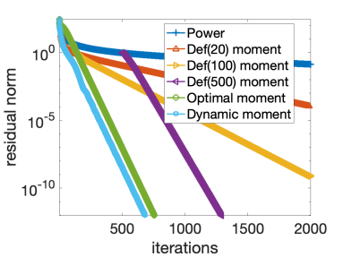
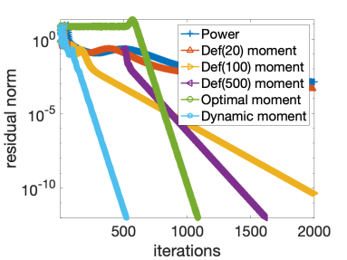
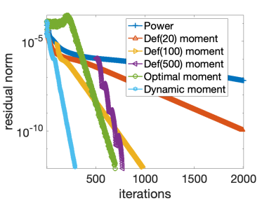
Figure 2 shows iteration count vs. the residual norm using algorithm 1.1, DMPOW with 20, 100 and 500 preliminary iterations, algorithm 1.2, and algorithm 3.3. Each iteration was started with the initial $u_{0}=\begin{pmatrix}1&1&\cdots&1\end{pmatrix}^{T}$. The preliminary iterations of DMPOW were started with $w_{0}=\begin{pmatrix}-1&1&-1&1\cdots\end{pmatrix}^{T}$, so that $w_{0}$ is orthogonal to $u_{0}$. In the first two cases, we see the dynamic method algorithm 3.3 converges at approximately the same asymptotic rate as algorithm 1.2, though in the second case the latter has an extended preasymptotic regime. The three DMPOW instances work essentially as they should for Matrix 1 and Matrix 2, where the approximation of $\lambda_{2}$ from the deflation method, hence the approximation of $\beta_{opt}=\lambda_{2}^{2}/4$ improves as the preliminary iterations are increased. For Matrix 1 DMPOW with 500 preliminary iterations does appear to achieve the optimal convergence rate. In Matrix 3 on the right, only the dynamic method algorithm 3.3 achieves a steady optimal convergence rate. Algorithm 1.2 initially stalls then achieves a good but sub-optimal rate. DMPOW with 500 preliminary iterations achieves an apparently optimal but oscillatory convergence rate, with sub-optimal rates with 100 and 20 preliminary iterations. The oscillatory behavior of DMPOW suggests that the approximation to $\lambda_{2}$ is greater than $\lambda_{2}$, hence all subdominant modes are oscillatory, via (2.9).

4.2 Test suite 2

The second test suite consists of four matrices. The first three are symmetric indefinite and the fourth is SPD with increasing gaps between the smaller eigenvalues.

Matrix 4:

$A=$ash292 from [6], with $n=292$. This matrix has leading eigenvalues $\lambda_{1}=9.1522$ and $\lambda_{2}=8.3769$, with $r=0.9153$. It is symmetric indefinite.

Matrix 5:

$A=$bcspwr06 from [6], with $n=1454$. This matrix has leading eigenvalues $\lambda_{1}=5.6195$ and $\lambda_{2}=5.5147$, with $r=0.9814$. It is symmetric indefinite.

Matrix 6:

$A=\operatorname{diag}($linspace$(-99,100,200))$. This matrix has $n=200$, $\lambda_{1}=100$, $\lambda_{2,3}=\pm 99$, and $r=0.99$. It is included to test the sensitivity to positive and negative leading subdominant eigenvalues.

Matrix 7:

$A=\operatorname{diag}(10-$logspace$(0,1,200))$. This matrix has $n=200$, $\lambda_{1}=9$, $\lambda_{2}=8.9884$, and $r=0.999$. It is included to test the sensitivity to increasing gaps between smaller eigenvalues.

	Matrix 4		Matrix 5		Matrix 6		Matrix 7
method	min	max	min	max	min	max	min	max
Power	247	359	1088	1583	2000	2000	2000	2000
DMPOW(20)	125	746	197	655	2040	2040	2040	2040
DMPOW(100)	340	376	415	1735	1281	2200	1318	2200
DMPOW(500)	1503	1503	1575	1626	1767	3000	1970	3000
$\beta=\lambda_{2}^{2}/4$	71	86	152	179	241	288	550	640
dynamic $\beta$	66	96	133	175	255	652	470	612

Table 1: Minimum and maximum number of matrix-vector multiplies to residual convergence for 100 runs of the power method (algorithm 1.1), DMPOW run with 20, 100 and 500 preliminary iterations, the power iteration with optimal momentum (algorithm 1.2) and the power iteration with dynamic momentum (algorithm 3.3), applied to Matrix 4 - Matrix 7. Each run used a randomly generated initial vector.

Results of the experiments with the second set of matrices is shown in table 1. We see that the dynamic algorithm 3.3 shows more sensitivity to initial vector than does the static algorithm with optimal parameter 1.2 in the indefinite cases, and particularly for the highly indefinite Matrix 6. From the results for Matrix 7, we see that increasing the spacing between the smaller eigenvalues does not cause increased sensitivity to $u_{0}$. We can also see that algorithms 1.2 and 3.3 significantly outperform the others on all tests in this suite.

4.3 Test suite 3

For the third test suite, we generated 100 symmetric matrices with unit diagonal, and quasi-randomly generated normally distributed off-diagonals with mean zero and standard deviation one, via v = ones(n,1); v1 = randn(n-1,1); A = diag(v,0) + diag(v1,1) + diag(v1,-1);. For each matrix, we checked the ratio $r=|\lambda_{2}/\lambda_{1}|$. Over the 100 matrices, the values of $r$ ranged from $0.7944$ to $0.9996$, with mean value $0.9491$ and standard deviation $0.0455$. Each run was started with the initial iterate $u_{0}=\begin{pmatrix}1&1&\cdots&1\end{pmatrix}^{T}$.

Table 2 shows the results. While algorithm 1.2 with optimal fixed $\beta$ has the lowest minimal number of iterations over 100 runs, dynamic algorithm 3.3 has the lowest mean and maximum iteration count. For these two methods the iteration count is the same as the reported number of matrix-vector multiplies. On the other hand, DMPOW with 20, 100 and 500 preliminary iterations each had at least one run that did not terminate after 2000 total iterations (preliminary included), and all three of the DMPOW methods had a substantially higher minimum number of matrix-vector multiplies than either the optimal or dynamic methods.

	Matrix-vector multiplies				Terminal residual
method	mean	std. dev.	min	max	min	max
Power	905.42	658.728	96	2000	8.74e-13	4.89e-04
DMPOW(20)	439.15	528.614	101	2040	6.31e-13	4.43e-04
DMPOW(100)	498.3	295.655	302	2200	2.15e-13	7.95e-12
DMPOW(500)	1600.55	196.335	1502	3000	1.78e-13	4.96e-06
$\beta=\lambda_{2}^{2}/4$	162.22	160.065	40	1183	6.02e-13	9.99e-13
dynamic $\beta$	150.15	133.842	63	949	5.66e-13	1.00e-12

Table 2: The number of matrix-vector multiplies and terminal residual for 100 runs of the power method (algorithm 1.1), DMPOW run with 20, 100 and 500 preliminary iterations, the power iteration with optimal momentum (algorithm 1.2) and the power iteration with dynamic momentum (algorithm 3.3). Each run used pseudo-randomly generated tridiagonal matrix v = ones(n,1); v1 = randn(n-1,1); A = diag(v,0) + diag(v1,1) + diag(v1,-1);, and the same initial vector $u_{0}=\begin{pmatrix}1&1&\cdots&1\end{pmatrix}^{T}$.

4.4 Test suite 4

In this fourth suite of tests, we consider three problems of varying structure and scale, and which have eigenvalues of varying magnitudes. The dynamic momentum algorithm 3.3 is tested against the power method 1.1, the static momentum algorithm 1.2 with optimal parameter $\beta=\lambda_{2}^{2}/4$, and perturbations thereof, $\beta_{-}=0.99\times\beta_{opt}$, and $\beta_{+}=\min\{1.01\times\beta_{opt},(3\lambda_{1}^{2}+\lambda_{2}^{2})/16\}$. The parameters $\beta_{+}$ and $\beta_{-}$ are within 1% of $\beta_{opt}$, but do not exceed $\lambda_{1}^{2}/4$, which as per section 2 would prevent convergence.

Matrix 8:

$A=$Si5H12 from [6], with $n=$ 19,896. This matrix has leading eigenvalues $\lambda_{1}=$58.5609 and $\lambda_{2}=$58.4205, with $r=0.998$. It is symmetric indefinite.

Matrix 9:

$A=$ss1 from [6], with $n$= 205,282. This matrix has leading eigenvalues $\lambda_{1}=1.3735$ and $\lambda_{2}=1.3733$, with $r=0.9998$. It is nonsymmetric.

Matrix 10:

$A=$thermomech_TC, with $n=$ 102,158. This matrix has This matrix has leading eigenvalues $\lambda_{1}=0.03055$ and $\lambda_{2}=0.03047$, with $r=0.9975$. It is SPD.

Figure 3: Convergence of the residual by iteration count for the three matrices in test suite 4, using algorithm 1.1, algorithm 1.2 with $\beta=\beta_{opt}=\lambda_{2}^{2}/4$, with $\beta=\min\{1.01\times\beta_{opt},(3\lambda_{1}^{2}+\lambda_{2}^{2})/16\}$, $\beta=0.99\times\beta_{opt}$, and and algorithm 3.3. Left: Matrix 8, Si5H12; center: Matrix 9, ss1; right: Matrix 10, thermomech_TC.

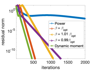
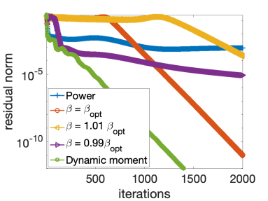
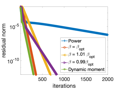
Convergence of the residual in each case is shown in figure 3. Each of the tests was started from the initial vector $u_{0}=\begin{pmatrix}1&1&\cdots&1\end{pmatrix}^{T}$. The results show the dynamic method 3.3 is not sensitive to the scaling of the eigenvalues which vary in each of the examples. The results also show a better rate of convergence with $\beta_{+}$ than with $\beta_{-}$, but at the cost of a potentially extended preasymptotic regime. For ss1 (Matrix 9) shown in the center plot, the dynamic method shows some initial oscillations but does not suffer for the extended asymptotic regime that $\beta_{opt}$ and $\beta_{+}$ experience.

5 Dynamic Momentum Method for Inverse Iteration

As an immediate extension of algorithm 3.3, this section explores the application of the dynamic momentum method to accelerate the shifted inverse power iteration. The shifted inverse iteration is a well-known and powerful technique in the numerical solution of eigenvalue problems. A review of the method including its history, theory and implementation can be found in [14]. By appropriately choosing shifting parameters, the inverse iteration with shift can be used to identify any targeted eigenpair. When a good approximation of the targeted eigenvalue is available, the method is remarkably efficient. As the inverse iteration with shift $\sigma$ is equivalent to applying the power iteration on the matrix $(A-\sigma I)^{-1}$ (with the same eigenvectors as those of $A$), the analysis carried out in section 3.1 is directly applicable to the algorithm 5.5 below.

Each step of the inverse iteration involves solving a linear system. For a fixed shift, one can perform a factorization of the shifted matrix before the iterative loop to save some computational cost. Unlike updating the shift to attain faster convergence, applying a momentum acceleration does not require a re-factorization of the matrix. As shown below, the momentum accelerated algorithm substantially reduces the number of iterations to convergence, particularly for sub-optimal shifts. Presumably, the use of a sub-optimal shift indicates the user does not have a good approximation of the target eigenvalue, by which the user is unlikely to have a good approximation of the second eigenvalue of the shifted system. Hence the automatic assignment of the extrapolation parameter $\beta_{k}$ is essential for this method to be practical. Fortunately, as seen below, the proposed method with dynamic $\beta_{k}$ at least slightly outperforms the optimal parameter in each case tested. Numerical experiments below illustrate the improved efficiency, particularly with the dynamic strategy.

Just as algorithm 3.3 requires two preliminary power iterations, the dynamic momentum strategy for the inverse iteration requires two preliminary inverse iterations. For tests in this section, we ran iterations to a residual tolerance of $10^{-15}$ or a maximum of 2000 iteration. In this section we also numerically verify the stability of the extrapolation parameter $\beta_{k}$ as shown in lemma 3.4 and remark 3.5.

Algorithm 5.4.

Inverse power iteration

Choose $v_{0}$ and shift $\sigma$, set $h_{0}=\left\|{v_{0}}\right\|$ and $x_{0}=h_{0}^{-1}v_{0}$

Compute $(A-\sigma I)=LU$ $\triangleright$ Compute LU factors of $A-\sigma I$

Solve $Ly=x_{0}$ and $Uv_{1}=y$

for $k\geq 0$ do

     Set $h_{k+1}=\left\|{v_{k+1}}\right\|$ and $x_{k+1}=h_{k+1}^{-1}v_{k+1}$

     Solve $Ly=x_{k+1}$ and $Uv_{k+2}=y$

     Set $\nu_{k+1}=(v_{k+2},x_{k+1})$ and $d_{k+1}=\|v_{k+2}-\nu_{k+1}x_{k+1}\|$

     STOP if $\left\|{d_{k+1}}\right\|<$ tol

end for

The dynamically accelerated version of algorithm 5.4 follows.

Algorithm 5.5.

Dynamic momentum for inverse iteration

Do two iterations of algorithm 5.4 $\triangleright$ $k=0,1$

Set $r_{2}=\min\{d_{2}/d_{1},1\}$

for $k\geq 2$ do $\triangleright$ $k\geq 2$

     Set $\beta_{k}=\nu_{k}^{2}r_{k}^{2}/4$

     Set $u_{k+1}=v_{k+1}-(\beta_{k}/h_{k})x_{k-1}$

     Set $h_{k+1}=\left\|{u_{k+1}}\right\|$ and $x_{k+1}=h_{k+1}^{-1}u_{k+1}$

     Solve $Ly=x_{k+1}$ and $Uv_{k+2}=y$

     Set $\nu_{k+1}=(v_{k+2},x_{k+1})$ and $d_{k+1}=\left\|{v_{k+2}-\nu_{k+1}x_{k+1}}\right\|$

     Update $\rho_{k}=\min\{d_{k+1}/d_{k},1\}$ and $r_{k+1}=2\rho_{k}/(1+\rho_{k}^{2})$

     STOP if $\left\|{d_{k+1}}\right\|<$ tol

end for

In table 3 we show results for accelerating the inverse iteration used to recover the largest eigenvalue of the matrix $A=\operatorname{diag}(1000:-1:1)$. We test shifts $\sigma=\{999.75,\ldots,1004\}$, chosen with increasing distance from the target eigenvalue $\lambda_{1}=1000$ to see how much a suboptimal shift can be made up for with the extrapolation. We see the dynamic momentum method gives the best performance in each case, and the “optimal” fixed parameter gives a good performance, but it is outperformed in some cases by a nearby static shift as well as the dynamic shift. Compared with the base algorithm 5.4, algorithm 5.5 with dynamically chosen $\beta_{k}$ not only reduces the number of iterations for each given shift, it also achieves a better iteration count with shifts more than twice as far away from the target eigenvalue. This shows algorithm 5.5 reduces the sensitivity to the shift in the standard inverse iteration.

	$0$	dyn $\beta_{k}$	$\beta_{opt}$	$0.01$	$0.02$	$0.04$	$0.08$	$0.16$	$0.32$	$0.64$
999.75	32	21	23 (0.44)	32	32	31	31	30	27	23
1000.25	22	16	18 (0.16)	22	22	21	20	18	19	22
1000.5	32	21	23 (0.11)	31	31	30	27	23	29	42
1001	50	29	34  (0.063)	48	46	41	30	43	92	–
1002	86	42	52  (0.032)	75	64	44	95	–	–	–
1004	155	69	88  (0.012)	88	97	–	–	–	–	–
1009	328	146	175  (0.0025)	–	–	–	–	–	–	–

Table 3: Shifted inverse iteration to find the largest eigenvalue with fixed and dynamic momentum for the matrix $A=\operatorname{diag}(n:-1:1)$, with $n=1000$. The optimal fixed extrapolation parameters $\beta_{opt}=1/(4(\lambda_{2}-\sigma)^{2})$ is shown after the iteration count in the $\beta_{opt}$ column, and the dynamically chosen parameter $\beta_{k}$ is set as in algorithm 5.5. No convergence is obtained for $\beta>1/(4(\lambda_{1}-\sigma)^{2})$, as explained by (2.11). Each iteration is started from $v_{0}=\begin{pmatrix}1&1&\cdots&1\end{pmatrix}^{T}$, and run to a residual tolerance of $10^{-15}$.

Figure 4: Behavior of $\beta_{k}$ with respect to $\beta_{opt}$ for representative examples from table 3, illustrating that $\beta_{k}$ stabilizes closer to $\beta_{opt}$ in agreement with lemma 3.4 as $r\rightarrow 1$. Left: $\sigma=1001$, for which $r=0.5$. Center: $\sigma=1004$, for which $r=0.8$. Right: $\sigma=1009$ for which $r=0.9$.

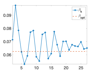
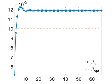
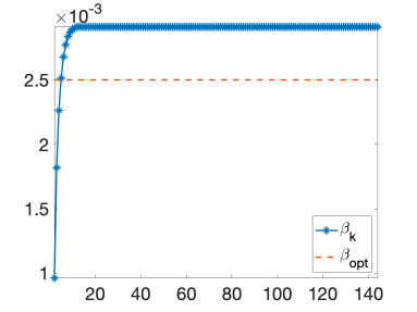
Figure 4 shows the extrapolation parameters $\beta_{k}$ for three different shifts $\sigma$ as shown in table 3. The left plot shows $\{\beta_{k}\}$ for $\sigma=1001$. Denoting the eigenvalues of $(A-\sigma I)^{-1}$ as $\{\tilde{\lambda}_{i}\},i=1,\ldots,n$, we have $\tilde{\lambda}_{1}=-1$, and $\tilde{\lambda}_{2}=-1/2$ so that $r=0.5$. In this case $\beta_{k}$ oscillates above and below $\beta_{opt}$. For $\beta_{k}<\beta_{opt}$, $\tilde{\lambda}_{2}$ is non-oscillatory by (2.9), but each of the eigenvalues with $\tilde{\lambda}^{2}/4$ is oscillatory, and each decays at a slightly faster rate than $\tilde{\lambda}_{2}$ by (2.11). As per lemma 3.4, the approximation of $r$ by the detected convergence rate $\rho_{k}$ is stable, but the oscillations in $r_{k+1}$ are not necessarily damped with respect to the detected $\rho_{k}$. For $\beta_{k}>\beta_{opt}$, all subdominant modes are oscillatory and decay at the same rate by (2.11), and the stability of $r_{k+1}$ with respect to $\rho_{k}$ still holds. For the center plot in figure 4, $\sigma=1004$ so that $r=0.8$; and in the right plot $\sigma=1009$ so that $r=0.9$. In both of these cases, lemma 3.4 shows that $r_{k+1}$ is stable with respect to $\rho_{k}$, and the difference between $r_{k}$ and $r$ is damped in comparison to the difference between the detected $\rho_{k}$ and $\rho$; and moreso in the plot on the right with $r=0.9$. For $r$ closer to unity, the difference in the convergence rates between $\tilde{\lambda}$ with $\tilde{\lambda}^{2}/4>\beta_{k}$ and $\tilde{\lambda}^{2}/4<\beta_{k}$ become more substantial so the eigenmode associated with $\tilde{\lambda}_{2}$ dominates the residual, which causes $\beta_{k}$ to settle above $\beta_{opt}$. Notably for the center figure with $r=0.8$, $\beta_{k}$ settles approximately $2\times 10^{-3}$ above $\beta_{opt}$. For the right plot with $r=0.9$, $\beta_{k}$ settles approximately $0.5\times 10^{-3}$ above $\beta_{opt}$, which demonstrates how $r_{k}$ relaxes towards $r$ as $r$ approaches one, as described in lemma 3.4.

	$0$	dyn $\beta_{k}$	$\beta_{opt}$	1e-4	1e-3	1e-2	1e-1	2e-1	4e-1	8e-1
1.25	32	21	23 (4.4e-1)	32	32	32	31	29	25	24
0.75	22	16	17 (1.6e-1)	22	22	22	20	17	19	24
0.5	32	21	23 (1.1e-1)	32	32	31	25	25	32	50
0	50	29	33 (6.3e-2)	50	50	48	33	51	170	–
-1.0	86	42	52 (2.8e-2)	86	85	75	175	–	–	–
-3.0	155	69	87 (1.0e-2)	155	149	87	–	–	–	–
-7.0	294	130	157 (1.3e-3)	290	251	–	–	–	–	–
-15.0	570	265	296 (8.7e-4)	539	249	–	–	–	–	–

Table 4: Shifted inverse iteration to find the smallest eigenvalue with fixed and dynamic momentum for the matrix $A=\operatorname{diag}(n:-1:1)$, with $n=1000$. The optimal fixed extrapolation parameters $\beta_{opt}=1/(4(\lambda_{n-1}-\sigma)^{2})$ is shown after the iteration count in the $\beta_{opt}$ column, and the dynamically chosen parameter $\beta_{k}$ is set as in algorithm 5.5. No convergence is obtained for $\beta>1/(4(\lambda_{n}-\sigma)^{2})$, as explained by (2.11). Each iteration is started from $v_{0}=\begin{pmatrix}1&1&\cdots&1\end{pmatrix}^{T}$, and run to a residual tolerance of $10^{-15}$.

Figure 5: Residual convergence for representative examples from table 4, illustrating the improvement in convergence for the optimal and dynamic momentum acceleration for a variety of shifts. Left: $\sigma=1.25$, for which $r=1/3$. Center: $\sigma=0$, for which $r=0.5$. Right: $\sigma=-3$ for which $r=0.8$.

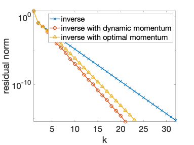
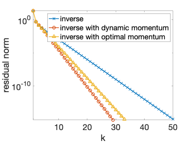
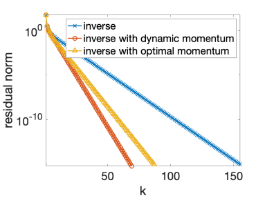
In table 4 we show the results of a similar experiment to recover the smallest eigenvalue of the matrix $A=\operatorname{diag}(1000:-1:1)$. We test shifts $\sigma=\{1.25,0.75,0.5,0,-1,-3,-7,-15\}$, a range of shifts with increasing distance from the target eigenvalue $\lambda_{n}=1$. Our results are similar to the largest eigenvalue case of table 3. As the distance between the target eigenvalue and the shift increases, the dynamic methods takes less than half the iterations of the standard inverse iteration, and in another view, it converges in fewer iterations than the standard inverse iteration does with a shift twice as close to the target eigenvalue. In each case, the dynamic method outperforms all of the static shifts. Figure 5 shows convergence plots for $\sigma=1.25,\sigma=0$ and $\sigma=-3$, providing a visualization of the improved convergence rates from the dynamic algorithm 5.5. These examples illustrate the gain in convergence from this practical and low-cost acceleration method.

6 Conclusion

In this paper we introduced and analyzed a one step extrapolation method to accelerate convergence of the power iteration for real, diagonalizable matrices. The method is based on the momentum method for the power iteration introduced in [22], and requires a single matrix-vector multiply per iteration. Unlike the method of [22] and other recent variants such as [21], the presently introduced technique gives a dynamic update of the key extrapolation parameter at each iteration, and does not require any a priori knowledge of the spectrum.

We first reviewed some results on the analysis of a static method of the form introduced in [22], by considering the power iteration applied to an augmented matrix. Our analysis goes beyond that shown in the original paper, revealing that the augmented matrix is defective for the optimal parameter choice, which explains why slower convergence is expected in the preasymptotic regime. We then analyzed our dynamic method showing both stability of the dynamic extrapolation parameter and convergence of the method.

In the last two sections we numerically demonstrated the efficiency of the introduced dynamic algorithm 3.3 as applied to power and inverse iterations. We demonstrated that algorithm 3.3 often outperforms the original static method with the optimal parameter choice as given in algorithm 1.2. We further showed algorithm 3.3 performs favorably in comparison to the method of [21], which generally accelerates the power iteration but does not exceed the performance of algorithm 1.2. Finally, we showed that the introduced dynamic method is a useful tool to accelerate inverse power iterations, and can be used to converge in as few iterations as having a shift twice as close to the target eigenvalue, and without significant additional computational complexity. Future work will include the development of an analogous method applied to (preconditioned) Krylov subspace projection methods as in [10, 16, 18, 20] to efficiently recover multiple eigenpairs.

7 Acknowledgements

CA and SP are supported in part by NSF DMS-2045059 (CAREER). This material is based upon work supported by the NSF under DMS-1929284 while SP was in residence at the Institute for Computational and Experimental Research in Mathematics in Providence, RI, during the Numerical PDEs: Analysis, Algorithms and Data Challenges Program. SP would also like to thank Prof. Nilima Nigam for many interesting discussions that led to the formulation of this work.

References

- [1] I. Babuška and J. Osborn. Eigenvalue problems. In P. G. Ciarlet and J. L. Lions, editors, Handbook of Numerical Analysis. II: Finite Element Methods (Part 1), pages 641–787. North-Holland, Amsterdam, 1991.
- [2] Z.-Z. Bai, W.-T. Wu, and G. V. Muratova. The power method and beyond. Applied Numerical Mathematics, 2020.
- [3] C. Brezinski. Computation of the eigenelements of a matrix by the -algorithm. Linear Algebra and its Applications, 11(1):7–20, 1975.
- [4] C. Brezinski and M. Redivo-Zaglia. The PageRank vector: properties, computation, approximation, and acceleration. SIAM J. Matrix Anal. Appl., 28:551–575, 2006.
- [5] E. R. Davidson. The iterative calculation of a few of the lowest eigenvalues and corresponding eigenvectors of large real-symmetric matrices. Journal of Computational Physics, 17(1):87–94, 1975.
- [6] T. A. Davis and Y. Hu. The University of Florida sparse matrix collection. ACM Transactions on Mathematical Software, 38(1):1–25, 2011.
- [7] J. A. Duersch, M. Shao, C. Yang, and M. Gu. A robust and efficient implementation of LOBPCG. SIAM Journal on Scientific Computing, 40(5):C655–C676, 2018.
- [8] G. H. Golub and C. Greif. An Arnoldi-type algorithm for computing page rank. BIT Numerical Mathematics, 46:759–771, 2006.
- [9] G. H. Golub and C. F. Van Loan. Matrix Computations (3rd Ed.). Johns Hopkins University Press, Baltimore, MD, USA, 1996.
- [10] G. H. Golub and Q. Ye. An inverse free preconditioned Krylov subspace method for symmetric generalized eigenvalue problems. SIAM Journal on Scientific Computing, 24(1):312–334, 2002.
- [11] T. H. Haveliwala, S. D. Kamvar, D. Klein, C. D. Manning, and G. H. Golub. Computing PageRank using power extrapolation, 2003. Technical report SCCM03-02, Stanford University, Stanford, CA.
- [12] M. Hochstenbach and Y. Notay. The jacobi–davidson method. GAMM-Mitteilungen, 29(2):368–382, 2006.
- [13] Q.-Y. Hu, C. Wen, T.-Z. Huang, Z.-L. Shen, and X.-M. Gu. A variant of the Power-Arnoldi algorithm for computing PageRank. Journal of Computational and Applied Mathematics, 381:113034, 2021.
- [14] I. C. F. Ipsen. Computing an eigenvector with inverse iteration. SIAM Review, 39(2):254–291, 1997.
- [15] S. Kamvar. Numerical Algorithms for Personalized Search in Self-organizing Information Networks. Princeton University Press, Princeton, 2010.
- [16] A. V. Knyazev. Toward the optimal preconditioned eigensolver: Locally optimal block preconditioned conjugate gradient method. SIAM Journal on Scientific Computing, 23(2):517–541, 2001.
- [17] N. Nigam and S. Pollock. A simple extrapolation method for clustered eigenvalues. Numerical Algorithms, 89:115–143, 2022.
- [18] S. Pollock and L. R. Scott. Extrapolating the Arnoldi algorithm to improve eigenvector convergence. International Journal of Numerical Analysis and Modeling, 18(5):712–721, 2021.
- [19] B. T. Polyak. Some methods of speeding up the convergence of iteration methods. USSR Computational Mathematics and Mathematical Physics, 45:1–17, 1964.
- [20] P. Quillen and Q. Ye. A block inverse-free preconditioned Krylov subspace method for symmetric generalized eigenvalue problems. Journal of Computational and Applied Mathematics, 233(5):1298–1313, 2010. Special Issue Dedicated to William B. Gragg on the Occasion of His 70th Birthday.
- [21] T. Rabbani, A. Jain, A. Rajkumar, and F. Huang. Practical and fast momentum-based power methods. In J. Bruna, J. Hesthaven, and L. Zdeborova, editors, Proceedings of the 2nd Mathematical and Scientific Machine Learning Conference, volume 145 of Proceedings of Machine Learning Research, pages 721–756. PMLR, 2022.
- [22] C. D. Sa, B. He, I. Mitliagkas, C. Ré, and P. Xu. Accelerated stochastic power iteration. Proc. Mach. Learn. Res., 84:58–67, 2019.
- [23] Y. Saad. Numerical methods for large eigenvalue problems: revised edition, volume 66. Society for Industrial and Applied Mathematics, Philadelphia, PS, USA, 2011.
- [24] A. Sidi. Approximation of largest eigenpairs of matrices and applications to Pagerank computation.
- [25] A. Sidi. Vector extrapolation methods with applications to solution of large systems of equations and to PageRank computations. Computers & Mathematics with Applications, 56:1–24, 2008.
- [26] J. H. Wilkinson. The Algebraic Eigenvalue Problem. Clarendon Press, Oxford, 1965.