Reawakening knowledge: Anticipatory recovery from catastrophic interference via structured training

Abstract

We explore the training dynamics of neural networks in a structured non-IID setting where documents are presented cyclically in a fixed, repeated sequence. Typically, networks suffer from catastrophic interference when training on a sequence of documents; however, we discover a curious and remarkable property of LLMs finetuned sequentially in this setting: they exhibit anticipatory behavior, recovering from the forgetting on documents before encountering them again. The behavior emerges and becomes more robust as the architecture scales up its number of parameters. Through comprehensive experiments and visualizations, we uncover new insights into training over-parameterized networks in structured environments. Code is available at https://github.com/Agentic-Learning-AI-Lab/anticipatory-recovery-public.

1 Introduction

(a) Loss on Document 1

(b) Shift-averaged loss

Figure 1: Loss curves for cyclic fine-tuning on the pre-trained Pythia-1b model, with 25 documents. The small black circles indicate points just prior to training on the focal task. These bell-shaped loss curves within each epoch demonstrate the anticipatory recovery phenomenon.

Large language models (LLMs) (Devlin et al., 2019; Brown et al., 2020; Touvron et al., 2023; OpenAI, 2023) have demonstrated remarkable general capabilities in a wide range of natural language tasks. During the training of LLMs, documents are typically uniformly sampled at random. Due to the large scale of the training set—in contrast to many other domains—LLM training typically occurs in an online fashion: each document is used only once for just one update step without further repetition (Hoffmann et al., 2022; Chowdhery et al., 2023; Xue et al., 2024).

Such a training style is in stark contrast with how real world agents like humans acquire new knowledge. In naturalistic settings, the material we’re exposed to is structured in time and often repeats. And given the cost of acquiring information in the real world, people aim to maximize their information gain from each episode. Obtaining new data is often associated with a cost, whether a mental switching cost—as when we go from one lecture to another—or a time cost of waiting for the information. In such scenarios, we hypothesize that real-world agents will spend more compute to best leverage each document than to switch among many.

Toward the goal of investigating more naturalistic training setups, we study a simplistic setting involving structured training of LLMs: documents are presented cyclically in a fixed sequence and are repeated multiple times, just as we humans go through our daily routines. Moreover, to account for the cost of switching among documents, we allow the network take multiple gradient steps for each document.

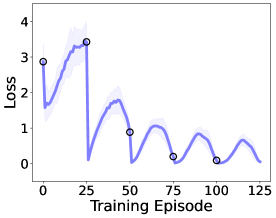
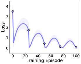
Typically, networks exhibit catastrophic interference (also known as catastrophic forgetting) (McCloskey and Cohen, 1989) when training on a sequence of tasks: the loss on a given document increases as the training advances to other documents. Surprisingly, we show that in a structured training environment, LLMs exhibit a curious anticipatory recovery behavior: they recover from the forgetting of one document before seeing it again, multiple steps in the sequence prior to the recurrence of the document (see Figure 1). It is analogous to a person anticipating to eat breakfast while taking a morning shower, but leaving the thought aside for the rest of the day. It is remarkable as there is no explicit memory in LLMs that stores sequential knowledge across documents, and there is no systematic overlap of content across documents—the behavior emerges from a random document sequence after repeated exposure to that sequence. Furthermore, only large scale networks reawaken their old knowledge during cyclic training, while smaller ones exhibit no such behavior.

Through extensive experiments, we study how different factors in model architecture and training contribute to the anticipatory recovery phenomenon. We offer insights on the training dynamics in sequentially and cyclically structured input data, and we propose hypotheses for the causes of the behavior. We also show that this phenomenon is not unique to LLMs; some vision models with sufficient width and depth also demonstrate a similar behavior, but LLMs on language modeling tasks exhibit the strongest recovery.

2 Data and Experiment Setup

In this section we describe the models, datasets, and training setups that we use in the subsequent LLM experiments. Additional details are presented in Appendix A.

Models.

We use Pythia (Biderman et al., 2023), a suite of decoder-only autoregressive language models pre-trained on the Pile dataset (Gao et al., 2020; Biderman et al., 2022). The Pythia suite has 8 models of different sizes. For our purposes, we use the five medium-sized models from 160M to 2.8B parameters. We use the fully pre-trained model (at 143K training steps) as well as the untrained initializations to study the effect of pre-training.

Datasets.

We use the CNN/Daily Mail news dataset (Nallapati et al., 2016). The dataset is originally designed for text summarization; we re-purpose it for causal language modeling by discarding the summaries and only using the articles as training data. Importantly, the CNN/Daily Mail dataset is not part of the Pile dataset and hence it is a new domain for the Pythia pre-trained models.

We use the same documents for both training and evaluation. Our goal here is not to determine whether a trained model generalizes to new documents, but rather to study the memory for a particular document as a function of position within the training history.

Training Setup.

We randomly sample $T$ documents from the CNN/Daily Mail news dataset. In pre-processing, we truncate each document and take only the first $C$ tokens (we refer to $C$ as “context length” in subsequent text). We then fine-tune our language model on each pre-processed sample for $M$ gradient steps (i.e., using a batch size of 1). We refer to the multiple gradient updates of each document as an “episode”. After each episode we evaluate the loss on all $T$ documents. We repeat the training process for $E$ epochs, where an epoch consists of one episode of each document in a fixed sequence. We use a vanilla gradient descent optimizer with learning rate $0.001$. Unless otherwise stated, the default hyper-parameters in the subsequent experiments are $T=25$, $C=256$, $M=10$, $E=5$. We use the average cross entropy loss (average negative log-likelihood for each token) as our training and evaluation metric. For all experiments we run 3 to 5 trials with different random seeds. The shaded area in the figures denotes standard deviation among trials.

3 Emergent Anticipatory Recovery

(a) Pre-trained Models

(b) Random Initializations

Figure 2: Effect of model size for (a) pre-trained models and (b) random initializations. In each subfigure, the left shows shift-averaged loss curves for five model sizes and the right shows the recovery score as a function of model size.

In this section, we present our experimental results that reveal the anticipatory recovery phenomenon in the cyclic fine-tuning of large language models. We then demonstrate that anticipatory recovery is an emergent behavior that appears only for models with sufficient capacity.

3.1 The Anticipatory Recovery Phenomenon

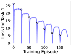
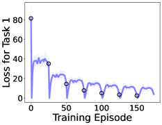
In this first experiment (Figure 1), we have $T=25$ documents, and we do cyclic fine-tuning on the documents for $E=5$ epochs in the same ordering. Both the documents and the ordering are sampled at random beforehand, but kept fixed during the sequential fine-tuning process. We refer to these $T$ documents as $\bm{x}_{1},\cdots,\bm{x}_{T}$. At the start, we fine-tune on document 1 for 10 gradient steps, leading to a significant decrease in the model’s loss on $\bm{x}_{1}$. As we move away from $\bm{x}_{1}$ and fine-tune on other documents, we naturally observe forgetting: the model’s loss on $\bm{x}_{1}$ gradually increases, due to catastrophic interference, until we finish fine-tuning on all other documents and return to $\bm{x}_{1}$. As we iterate through the same document sequence for a second time, we would normally expect the loss on $\bm{x}_{1}$ to still keep increasing after the initial decrease. However, Figure 1(a) shows that the loss on $\bm{x}_{1}$ peaks around $\bm{x}_{15}$ (episode 40) and then starts to decrease. Before we return to $\bm{x}_{1}$, it has recovered more than half of the model’s initial forgetting during the second epoch. We refer to this counter-intuitive decrease in loss as the anticipatory recovery phenomenon. In Figure 1(b), we plot the losses for all the documents and re-align them so that $0$ on the x-axis refers to the loss on each document $t$ immediately before training on it for the first time. The figure confirms that the anticipatory recovery phenomenon exists for not only $\bm{x}_{1}$ but all documents.

To quantify the strength of the anticipatory recovery phenomenon, we define the recovery score as the proportion of the initial forgetting during the current epoch that the model recovers before returning to the same document. Mathematically, let the mean (over $t$) of the maximum loss on each document $\bm{x}_{t}$ between the $n^{\text{th}}$ and $(n+1)^{\text{th}}$ time we train on that document be $l_{\text{max}}(n)$, right before the $(n+1)^{\text{th}}$ time we train on it be $l_{\text{before}}(n)$, and right after the $(n+1)^{\text{th}}$ time we train on it be $l_{\text{after}}(n)$. Then we define the recovery score (RS) for epoch $n$ to be

$$RS(n)=\frac{l_{\text{max}}(n)-l_{\text{before}}(n)}{l_{\text{max}}(n)-l_{\text{after}}(n-1)}.$$ (1)

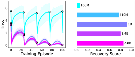
In the following subsections we compute the recovery scores for different model sizes and training hyper-parameters (Figures 2 and 5) to investigate their effects on the anticipatory recovery phenomenon.

3.2 Anticipatory Recovery is an Emergent Behavior

To study how the model size affects the amount of anticipatory recovery, we repeat this experiment with pre-trained Pythia models (Biderman et al., 2023) of different sizes, specifically 160M, 410M, 1B, and 2.8B. We plot the average loss curves as well as the recovery score for epoch 4 in Figure 2(a). We observe that larger models clearly demonstrate stronger anticipatory recovery. The sharp increase of average recovery score from the 160M model to the 410M model indicates that anticipatory recovery is an emergent behavior.

Anticipatory Recovery in Randomly Initialized Models.

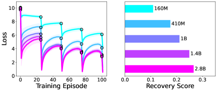
All our previous experiments are conducted with pre-trained language models. To study whether anticipatory recovery is a result of pre-training, we repeat the experiments on randomly initialized models of different sizes, and plot the loss curves and average recovery scores in Figure 2(b). We follow the model initialization recipe of Biderman et al. (2023). From the loss curves for the 410M and 1B model, especially in the last epoch, we see that the anticipation phenomenon also exists in randomly initialized LLMs. We observe that the anticipation effect is not as strong as in the pre-trained models. The effect of model size still holds: larger models clearly demonstrate stronger recovery.

Effects of Model Width and Depth.

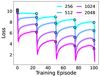
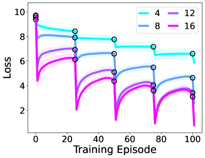
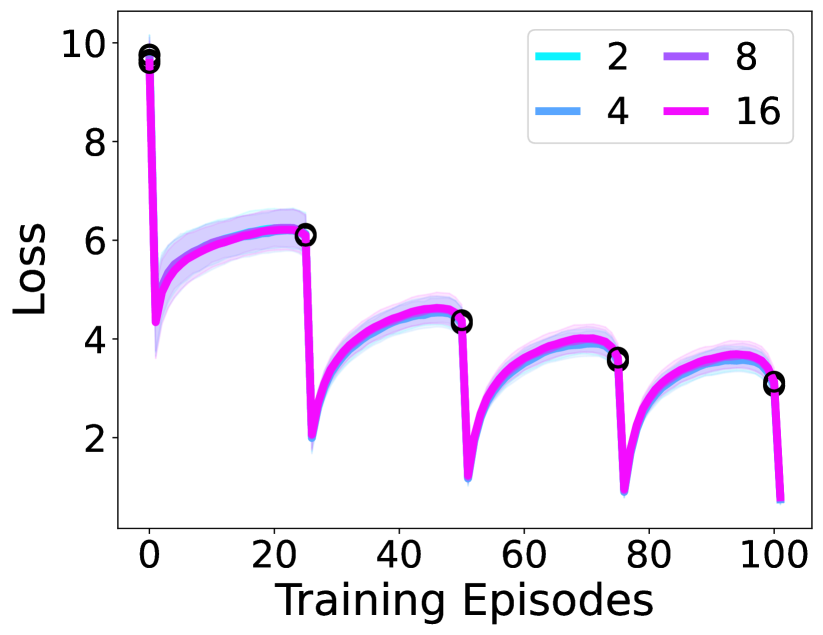
To further study the effect of model width and depth on the anticipatory recovery phenomenon beyond the model hyperparameters in the Pythia suite, we take a Pythia-1B model and vary the width (size of token embedding) and depth (number of transformer blocks) of the model and plot their average loss curves for cyclic training from random initializations in Figure 4. The original Pythia-1B model has token embedding of size 2048 and 16 transformer blocks. From the plots we observe that the model needs sufficient width (at least 512) and depth (at least 8 transformer blocks) to exhibit noticeable recovery, confirming that it is an emergent behavior contingent on model size.

(a) Size of Token Embedding

(b) Number of Model Blocks

Figure 3: Models trained from scratch with (a) different width (token embedding size) and (b) different depth (number of transformer blocks).

(c) Random Masking

(d) Random Window Shift

Figure 4: Effect of different levels of data randomization, with (a) random masking with probability up to $0.3$; (b) random shift of the context window up to $128$ tokens.

3.3 Other Influential Factors

In this section we discuss the effect of other training hyperparameters on the anticipatory recovery phenomenon. In each of the following paragraphs we vary one factor in the training setup and plot the different average loss curves for cyclic fine-tuning of a pre-trained Pythia-1B model. We also include some additional results in Appendix B.

(a) Number of Documents

(b) Number of Gradient Steps

(c) Context Length

(d) Number of Frozen Blocks

Figure 5: Effects of (a) number of documents (b) number of gradient steps (c) context length and (d) number of frozen blocks.

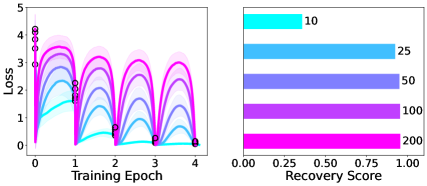
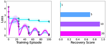
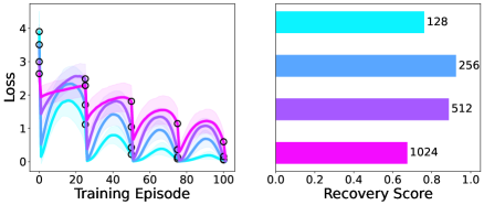
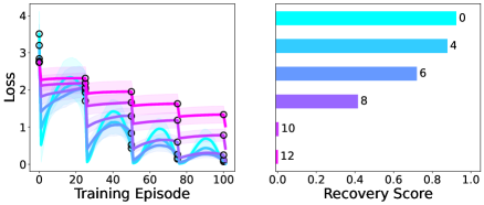
Number of Tasks.

We first try to increase the number of documents/tasks ($T$) the model is fine-tuned on in each epoch, with $T\in\{10,25,50,100,200\}$, and plot all the loss curves in Figure 5(a). From the figure we can observe clear recovery for all the curves, suggesting that the model can “memorize” a certain task transition even after training on 200 other tasks.

Number of Gradient Steps.

Figure 5(b) plots training curves with different numbers of gradient steps ($M$) taken on each task ($M\in\{1,5,10,20\}$). More gradient steps in general leads to higher recovery score, although in Appendix B.2 we show that slight anticipation is still observed for $1$ gradient step if we use a larger learning rate. We also demonstrate in the appendix that the anticipation effect is stronger when the same total update is divided among more gradient steps by scaling the learning rate inversely with $M$.

Context Length.

We experiment with different context lengths ($C\in\{128,256,512,1024\}$). Documents are padded to the same length with padding tokens. The loss curves are plotted in Figure 5(c). With the same number of gradient steps, larger context length is correlated with lower recovery score. This suggests that sufficient training on each task is necessary, and for longer input context it takes more gradient descent steps to memorize the task. For example, we show in Section B.6 that we can achieve the recovery score of context length 256 with $M=10$ for context length 1024 with $M=40$.

Number of Frozen Blocks.

We experiment with keeping only a subset of transformer blocks in the pre-trained model tunable and freezing the other layers during fine-tuning. Specifically, we freeze the first $B\in\{4,6,8,10,12\}$ transformer blocks (out of 16 total blocks in the Pythia-1B model) and tune only the last $16-B$ blocks. Loss curves are plotted in Figure 5(d). Results show that we need at least 8 tunable transformer blocks to observe a strong anticipation phenomenon in the last epoch. The results are consistent with our observations in section 3.2 and confirm that the model needs sufficient depth to exhibit anticipatory recovery even with a frozen pre-trained deep representation.

Optimizer.

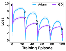
In addition to the gradient descent optimizer, we also experiment with the Adam optimizer (Kingma and Ba, 2015). For each document, we reset the optimizer state. Loss curves are plotted in Figure 6. Results show that Adam, which is a stronger optimizer than standard gradient descent, further facilitates anticipatory recovery, at least in part by producing greater initial forgetting. The average recovery score for Adam is $0.689$ while for vanilla gradient descent is $0.211$.

Data Randomness.

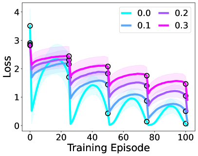
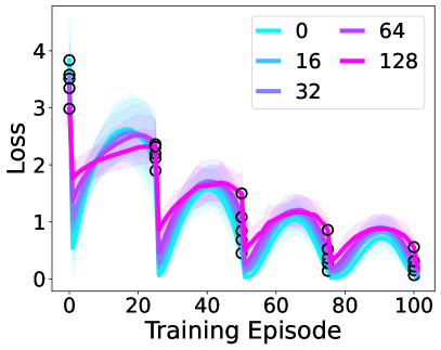
So far we have experimented with the exact same training documents across different epochs. However, in a more realistic sequential learning setting the data points might be slightly different for each repetition (e.g. different descriptions of the same concept, different perspectives of the same object), leading to stochasticity in the optimization process. To explore sequential cyclic training with data randomness, we design the following two training settings: for each gradient step on a document, we experimented with (1) randomly masking a subset (up to 30%) of the tokens in the input, and (2) randomly shifting the “window” of $C$ tokens used for training by up to $C/2$ tokens. The resulting loss curves are plotted in Figure 4. We observe that, while the anticipatory recovery phenomenon is generally weaker when there is more variation in each data point, the recovery still clearly exists.

Summary.

The experiment results in this subsection suggest that the model’s ability to fit on each task is crucial for the appearance of the anticipatory recovery phenomenon. With a larger number of gradient steps, shorter context length, more learnable layers, and a better optimizer, the model is more capable of fitting to the focal task, and those factors also correlate with larger recovery score. We also confirmed that anticipatory recovery exists for long task sequences and slightly augmented data points within each episode, and again these factors that make learning harder also reduce the anticipatory recovery.

Figure 6: Comparison between Adam and vanilla gradient descent optimizer for randomly initialized Pythia-1B models on cyclic training.

(a) Causal Image Modeling

(b) Image Classification

Figure 7: Results for cyclic training on vision tasks: (a) Causal image modeling with Image GPT. (b) image classification with vision transformers and VGG convolutional networks.

3.4 Anticipatory Recovery in Vision Models

To examine the generality of the anticipatory recovery phenomenon, in this subsection we explore the sequential cyclic training setting on two tasks in computer vision: causal image modeling and image classification. More detailed experiment setup is available in Appendix A.

Causal Image Modeling.

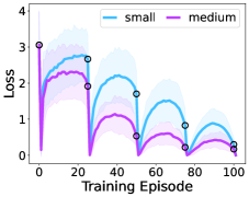
For the causal image modeling task, we use pre-trained Image GPT models and the corresponding pixel tokenizers from Chen et al. (2020), and we use CIFAR-10 (Krizhevsky et al., 2009) as the fine-tuning dataset. Similar to the LLM experiments, we fine-tune our model on each sampled image for $M$ gradient steps, and repeat $E$ epochs with a fixed order of the images. The resulting loss curves are shown in Figure 7(a). The results show that the anticipatory recovery phenomenon also exists for sequential cyclic training of image modeling in addition to language modeling.

Image Classification.

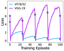
For the image classification task, we use pre-trained vision transformer (ViT) (Dosovitskiy et al., 2020) and VGG-19 (Simonyan and Zisserman, 2015) models, and we use ImageNet (Deng et al., 2009) as the training dataset. For each experiment, we randomly sample 800 images from Imagenet and divide them into 25 batches of 32 images each. We train our model on each batch for $M$ gradient steps and repeat $E$ epochs with a fixed order of the batches. The resulting loss curves are plotted in Figure 7(b). Results show that both the transformer ViT and the convolutional VGG exhibit anticipatory recovery in cyclic training.

By these experiments we confirm that anticipatory recovery occurs not only for LLMs but also for at least some of the widespread image classification models and non-transformer architectures.

4 Understanding Cyclic Training Dynamics

(a) Gradients

(b) Amount of Recovery

(c) Weights

(d) Activations

Figure 8: Heat map visualizations for (a) cosine similarities between the gradient vectors of the attention layer in transformer block 12 of the model for each task; (b) loss recoveries for training on task $\bm{x}_{i}$ (y-axis) and evaluating on task $\bm{x}_{j}$ (x-axis); (c) cosine similarities between the flattened model weight vectors at each point in training; (d) cosine similarities between the last layer activations for document $\bm{x}_{1}$ at each point in training.

An important general question about the anticipatory recovery phenomenon is whether it is due to some causal mechanism relating the dynamics of model parameters to the training sequence, or whether it is more correlational in that adjacent tasks come to be represented more similarly by the model. We found initial evidence for the latter hypothesis in experiments locally reversing the task sequence (e.g., showing that $x_{t+1}$ primes $x_{t}$ nearly as much as vice versa). To further test this learned similarity hypothesis, we explore the relationships between tasks and across training history of the model’s loss gradients, weights, and activations. The results enable us to better understand the dynamics of cyclic training. Unless otherwise stated, all visualizations in this section use the 410M model and default hyperparameters.

4.1 Temporal Structure of Gradients

We first explore the similarities of gradient information between documents during the training process. Our goal is to test the hypothesis that anticipatory recovery is mediated by increased similarity between gradients of proximal documents in our training sequence.

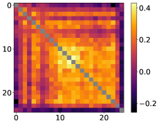
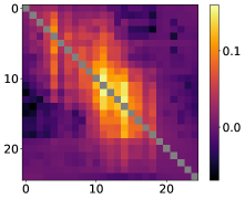
We do cyclic training for 4 epochs and compute the gradient of each document at the attention layer of transformer block 12 at the conclusion of training. In Figure 8(a), we plot the cosine similarities between these gradient vectors of each document. Results show that the gradients have mostly positive cosine similarities (except for the last document, on which the model has just been trained). We predicted the gradient similarities to depend only on $|i-j|$, peaking along the diagonal. Instead, to our surprise, the gradient similarities are highest near the center of the heat map. That is, the gradient similarity between documents $\bm{x}_{t-1}$ and $\bm{x}_{t}$ depends on where we are in the cycle. This result suggests an additional layer to the anticipatory recovery phenomenon: Recovery for document $\bm{x}_{t}$ is greatest from training on document $\bm{x}_{t-1}$, but the strength of the potential facilitation between $\bm{x}_{t-1}$ and $\bm{x}_{t}$ is actually greatest after we train for another $b$ documents (for some small number $b$, which ranges from roughly 10 to 15 in this particular case). We verify this by computing the pairwise recovery: we take the model checkpoint after 4 epochs of cyclic training, do $M$ gradient updates on document $\bm{x}_{i}$ and compute the difference in the loss of document $\bm{x}_{j}$ before and after these gradient updates, for each pair of documents $(\bm{x}_{i},\bm{x}_{j})$. We plot these pairwise loss recoveries in Figure 8(b). Results confirm that the amount of recovery on document $\bm{x}_{j}$ is highest when the model checkpoint is taken from roughly 10 to 15 documents before or after document $\bm{x}_{j}$ in cyclic training and then fine-tuned on a proximal document $\bm{x}_{i}$ in the sequence. The fact that this pairwise loss recovery matrix is roughly symmetric also suggests that the anticipatory recovery phenomenon approximately exhibits task symmetry: gradient updates on document $\bm{x}_{t}$ decrease the loss for document $\bm{x}_{t+k}$ for small integers $k$, and vice versa. We provide additional visualizations for $T=50,100,200$ in Appendix C and a more detailed description for this phenomenon.

Figure 9: Top three PCA components of last layer weights in the first three epochs.

(a) $f_{i}(\bm{w})=\bm{w}$

(b) $f_{i}(\bm{w})=\bm{y}_{i}-\bm{w}$

Figure 10: Loss curve for task 1 in computational toy model, with different $f_{i}$. More experiment details in Appendix A.3.

Figure 11: Visualization of PCA embeddings of the projected data points ($f_{i}^{-1}(\bm{P}\bm{x}_{i})$, where $f_{i}(\bm{w})=\bm{y}_{i}-\bm{w}$) in the toy model throughout training. Epoch 0 refers to the model before any training.

4.2 Temporal Structure of Model Weights

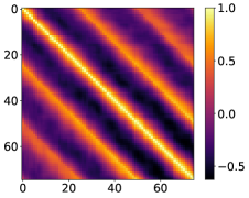
We explore the similarities of model weights along the optimization trajectory of cyclic training. We flatten and concatenate the weight vectors of the model checkpoint after we fine-tune on each document. However, the cosine similarities between these raw model weight vectors are all very close to 1 without obvious structure. This is mainly because of the proximity of model weights along the same optimization trajectory. Another reason is that the size of the weight vector is huge and dominated by a few entries, leading to numerical instability. To resolve these issues, we instead explore the structure of “weight residuals.” We compute the weight residuals by subtracting the average of weights in a window of length $T$ centered at the current document from the current weight, i.e.

$$w_{\text{res}}(t)=w(t)-\frac{1}{T}\sum_{n=t-T/2}^{t+T/2}w(n).$$ (2)

This removes the shared components along the optimization trajectory and allows us to focus on the model weight updates for each document. Figure 8(c) visualizes a heat map of the cosine similarity between each pair of weight residuals from the second epoch to the fourth epoch. The visualization shows a cyclic structure in the weight residuals, as equidistant bright stripes that align with the training epochs. Furthermore, each stripe spans several documents, suggesting the similarity of weight residuals for proximal documents.

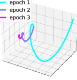
In addition to computing the cosine similarities between model weights, we explore using Principle Component Analysis (PCA) to reduce the dimensionality of the weights. We compute the top three PCs of the flattened last-layer weight vector (the output word embedding layer) for the Pythia-1B model, and plot its trajectory in Figure 9. The plot exhibits a clear helical structure that gradually converges. We believe this is highly relevant to anticipatory recovery: right before revisiting a task, the projected model weights in the helix move closer to the point corresponding to the previous appearance of that task, leading to anticipatory recovery on the loss of that task. As we go on with cyclic training, the model also exhibits less forgetting and gradually converges to a solution that achieves low loss on all tasks.

It is important to note that the helical structure of the weight trajectory is not an obviously necessary consequence of the cyclical training. Cyclical training could be expected to yield a repeating pattern, but the facts that the tasks come to be organized in a circle that respects their ordering and that the trajectory goes through one full revolution per epoch (rather than some other arc length) are nontrivial and seem to be essential for anticipatory recovery.

4.3 Temporal Structure of Activations

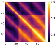
In addition to gradients and weights, we visualize the trajectory of activations on a single document during the course of cyclic training. We do cyclic training for three epochs and save model checkpoints after fine-tuning on each document. We then compute the model activations before the output word embedding layer for document $\bm{x}_{1}$ on each model checkpoint, and plot the cosine similarities between the flattened activation vectors in Figure 8(d). From the plot we can clearly observe the blocked pattern wherein the similarity between the activations become progressively higher across each epoch of cyclic training. This pattern suggests that every time we train on document $\bm{x}_{i}$, the internal representation of $\bm{x}_{i}$ in the model is more resistant to gradient updates on other documents $\bm{x}_{j}$.

4.4 Computational Toy Model

To further understand the essential mechanism that yields anticipatory recovery, we design a minimalist “toy” simulation experiment. In this toy simulation, each task (formerly, document) $i\in\{1,\cdots,T\}$ is described by a single data point, $\bm{x}_{1},\cdots,\bm{x}_{T}\in\mathbb{R}^{N}$. We assume a learnable linear embedding $\bm{P}\in\mathbb{R}^{M\times N}$ that projects each $\bm{x}_{i}$ into an $M$-dimensional embedding space. We also assume a learnable vector $w$ and task specific mappings $f_{i}$, where $f_{i}(w)$ is the target for task $i$ in the same embedding space. We require each $f_{i}$ to be invertible as a simplifying assumption.

We define the loss for task $i$ as

$$\ell_{i}(\bm{P},\bm{w})=\frac{1}{2}\lVert\bm{P}\bm{x}_{i}-f_{i}(\bm{w})\rVert^{2}_{2}.$$ (3)

Just as when training a deep net, we assume here that representation learning occurs slowly, and that one training step for task $i$ involves a single gradient update of $\bm{P}$ with step size $\alpha$:

$$\bm{P}\leftarrow\bm{P}-\alpha(\bm{P}\bm{x}_{i}-f_{i}(\bm{w}))\bm{x}_{i}^{\top}.$$ (4)

In contrast, at each training step, $\bm{w}$, analogous to the fast-adapting weights in a neural network, can be rapidly tuned to solve for task $i$, yielding the loss minimizer conditional on $\bm{P}$:

$$\bm{w}\leftarrow f_{i}^{-1}(\bm{P}\bm{x}_{i}).$$ (5)

As in our main experiments, we sequentially optimize each $\ell_{i}$ as we iterate through the sequence of tasks. In each training step, we first update $\bm{P}$ and then solve for $\bm{w}$ given the update to $\bm{P}$. In essence, updating $\bm{P}$ approximately reduces the distance between $\bm{P}\bm{x}_{i+1}$ and $f_{i+1}(f_{i}^{-1}(\bm{P}\bm{x}_{i}))$. Assume each $f_{i}$ is Lipschitz, then this will entail bringing $f_{i+1}^{-1}(\bm{P}\bm{x}_{i+1})$ toward $f_{i}^{-1}(\bm{P}\bm{x}_{i})$. As a result of this optimization objective, the model will evolve along the optimization trajectory such that the $f_{i}^{-1}(\bm{P}\bm{x}_{i})$ for all tasks $i$ gradually form a circular pattern. This gives an intuitive explanation on the anticipatory recovery phenomenon, since updaing $\bm{w}$ according to equation 5 will also bring it closer to $f_{i+1}^{-1}(\bm{P}\bm{x}_{i+1})$, thus reducing the loss on task $i+1$ and exhibits anticipatory recovery.

We experimented with two very simple choices of $f_{i}$: $f_{i}(\bm{w})=\bm{w}$ and $f_{i}(\bm{w})=\bm{y}_{i}-\bm{w}$ for some task-dependent targets $\bm{y}_{i}$. We follow the same order over tasks—$1,\cdots,T$—for multiple epochs of training. The resulting loss curves are shown in Figure 10, which exhibits very similar anticipatory recovery trajectory as the full-blown LLM experiment. Visualizations of the 2-dimensional PCA embeddings for $f_{i}^{-1}(\bm{P}\bm{x}_{i})$ in the second experiment are shown in Figure 11, which confirms our analysis that they gradually self-organize into a cyclic structure.

There are two potential reasons large overparameterized networks might produce the anticipatory recovery in a way analogous to the toy simulation. First, as the scale of the network grows, it is likely that the network can develop task-specific parameters that quickly adapt to and memorize the new input data, corresponding to Equation 5. And when the fast memorization is achieved, the gradient descent dynamics of the slow weights push the representations of the two adjacent tasks ($P\bm{x}_{i}$ and $P\bm{x}_{i+1}$) closer when $f$ is an identity function, according to Equation 4. In earlier LLM experiments, this effect can be seen in Figure 2, where larger models achieve significantly lower losses within a few gradient update steps during sequential learning. Second, larger networks have more learning capacity to map the features of two adjacent tasks closer. In our linear projection model, anticipatory recovery keeps growing over many epochs, whereas in LLM experiments, the anticipatory effect is already at the strongest within two or three epochs. Moreover, in the toy model all data points are randomly generated, which makes it easier to separate and map their representations according to a temporal structure than real-world data. In contrast, real-world data could require even more representation capacity since data points are noisy and correlated.

4.5 Summary

In this section, we visualized model weight dynamics with heatmaps and we showed model activations and gradients during cyclic training. We discussed the special temporal structure that is exhibited in these heat maps. We also plotted the pairwise degree of recovery for fine-tuning on document $i$ and evaluating on document $j$, as well as the change of distance between fine-tuned model weights on different tasks. The results suggest that after we train on a document, the model’s representation of that document becomes less sensitive to gradient updates on other documents. Finally, we showed a simple toy experiment that demonstrates a similar anticipatory recovery phenomenon in its loss curve, and discuss its connections to neural network training dynamics through the lens of task-specific and task-general parameters. Overall, these results shed some light on the dynamics of cyclic training.

5 Related Work

Cyclic and Structured Training.

Prior theoretical works have studied convergence rates, under various assumptions, for the training setup where the data points are shuffled only once and that order is reused for all epochs (Ahn et al., 2020; Gurbuzbalaban et al., 2019; Mishchenko et al., 2020; Safran and Shamir, 2020). On the empirical side, Xu et al. (2022) found that shuffling the data only once in the beginning can achieve a convergence rate comparable to shuffling every epoch. The training setup is equivalent to our cyclic training setup, but our research examines the loss on each task throughout the training cycle and discovers the anticipatory recovery effect. We also extend it to multiple gradient update steps on each data point.

Our research also relates to the more general topic of learning in structured environments. Jones et al. (2023) studied regression and classification tasks with multi-scale temporal structure in the environment characterized by $1/f$ dynamics. While the cyclic training setting that we study is a more simplified setup than that of Jones et al. (2023), we aim at unveiling more insights on applying standard SGD on over-parameterized networks. A potential direction for future work would be to study anticipatory recovery in regimes with richer, hierarchical sequence structure.

Online Learning.

Online learning deals with the setting where the tasks come from an online sequential stream. One of the simplest algorithms in online learning is follow-the-leader (Hannan, 1957), which stores all previous data from the stream and minimizes the total loss. It has strong performance guarantees but is computationally very expensive, and it also might not be feasible to store all the past data. Many subsequent works have developed cheaper algorithms under different assumptions (Zinkevich, 2003; Cesa-Bianchi and Lugosi, 2006; Shalev-Shwartz et al., 2012). Many recent works also explore the connection between online learning and meta-learning or continual learning (Denevi et al., 2019a; Finn et al., 2019; Denevi et al., 2019b; Javed and White, 2019; Fini et al., 2020; Ren et al., 2021; Wang et al., 2021).

The cyclic training setting that we explore in this research can be considered as a special case of the online learning setting where the data stream has a cyclic repetition structure. We employ multiple steps of online gradient descent (Biehl and Schwarze, 1995) on each document from the stream and study the training dynamics of over-parameterized neural networks.

LLM Emergent Capabilities.

Recent advancements in large-scale Transformer networks (Vaswani et al., 2017; Devlin et al., 2019) have demonstrated exceptional ability to model long sequence language data. Beyond basic language modeling and downstream task performance, these models have shown emergent behaviors (Wei et al., 2022a) that appear to manifest only beyond a certain model scale (Brown et al., 2020; Wei et al., 2022b; Ganguli et al., 2022; Srivastava et al., 2022).

Related to our research, recent studies reveal that LLMs possess remarkable memorization skills, enabling them to recall news sentences after just a few exposures (Biderman et al., 2023; Carlini et al., 2023; Orhan, 2023). However, the sequential learning dynamics behind such memorization have not been thoroughly examined. Our work comprehensively explore the sequential learning setting with cyclic task repetition and demonstrates task anticipation, a new emergent capability of large models.

Catastrophic Interference.

Traditionally, neural networks are trained for a single objective or task. However, when transitioning between tasks sequentially, they often experience “catastrophic interference” (McCloskey and Cohen, 1989), marked by a significant drop in performance on previously learned tasks. Continual learning (Van de Ven et al., 2020), a subset of machine learning, addresses a simplified setup where a model sequentially learns a set of tasks without revision. Numerous algorithms have been proposed to mitigate catastrophic forgetting, focusing on methods like parameter regularization (Kirkpatrick et al., 2017; Zenke et al., 2017; Aljundi et al., 2018), data replay (Rebuffi et al., 2017; Rolnick et al., 2019; Chaudhry et al., 2019), knowledge distillation (Hinton et al., 2015; Li and Hoiem, 2017; Buzzega et al., 2020; Madaan et al., 2023), and architectural isolation and expansion (Yoon et al., 2018; Serra et al., 2018; Gurbuz and Dovrolis, 2022; Kang et al., 2022).

More recently, there have been debates over the practicality of continual learning setups. Studies like Davidson and Mozer (2020) have shown that as networks learn more tasks, they improve in learning speed and reduce forgetting. In large models, studies suggest that pre-trained vision classifiers can undertake continual learning with ease, by either freezing or fine-tuning representations (Janson et al., 2022; Lee et al., 2023; Fini et al., 2022). In the language domain, research also suggests that LLMs exhibit emerging continual learning capabilities (Scialom et al., 2022; Ke et al., 2022).

Unlike prior literature on continual learning, our research uniquely focuses on sequential learning environments with cyclic repetition. Our work extends interleaved training (Mayo et al., 2023) to a larger number of tasks, specifically investigating the emergent anticipatory recovery phenomenon in cyclic training. This finding adds to the above literature by demonstrating a new mechanism by which large networks can avoid or recover from catastrophic interference.

6 Discussion

In this work, we explored the training dynamics of overparametrized neural networks, especially LLMs, in sequential cyclic fine-tuning, where a finite set of documents are presented in the same order within each epoch. We demonstrated the remarkable phenomenon of anticipatory recovery—networks recover from the initial forgetting before seeing the same document again. The effect holds across many different network instances and training hyper-parameters. This phenomenon is a sharp contrast with the well known phenomenon of catastrophic interference, where forgetting increases monotonically as a network is trained on a sequence of different documents.

We showed that anticipatory recovery occurs only when the network has sufficient width and depth and when it is well fitted to each document before moving to the next. We also discussed the effect of other important factors that influence the degree of recovery, such as the optimizer. Visualizations of model weights, model activations, and gradients exhibit clear temporal structure, which provide insights on the underlying mechanisms of anticipatory recovery. Our computational toy model decouples the shared representations from task-specific parameters and reproduces the phenomenon; however, the mathematical foundation of anticipatory recovery requires further investigation. Additionally, the toy model does not explain why the effect is stronger in LLMs in autoregressive tasks than in other types of architecture or learning objectives.

The cyclic training setup investigated in this work is distinct from the IID training setting assumed in the vast majority of the machine learning literature. It accounts for task repetition and task switching costs, which are critical components of the learning experience of humans and other real world agents. However, our current setup is still highly simplified from real world experience. We have yet to perform experiments on more naturalistic environments with sequential structures. Future research could investigate the emerging training dynamics of neural networks in different types of structured environments, such as multiscale temporal dynamics (Jones et al., 2023), from both theoretical and empirical perspectives.

Designing good learning curricula that achieve both learning efficiency and a low task-switching cost is a promising future direction that can be applied to more naturalistic training setups. On the modeling side, it will be worthwhile to rethink classic continual learning algorithms through the lens of LLMs and exploit and improve their emergent sequential memorization capability.

Appendix A Additional Experiment Setups

A.1 Causal Image Modeling Experiments

Models

Image GPT (Chen et al., 2020) is a GPT-2-like model trained to predict the next pixel value in an image. It is pre-trained on the Imagenet dataset (Deng et al., 2009) resized to 32x32. The Image GPT authors provide three pre-trained models of different sizes. In our experiments, we use the Image GPT-small and Image GPT-medium models.

Datasets

We use the CIFAR-10 (Krizhevsky et al., 2009) dataset for fine-tuning. For tokenization, the pixel RGB values are categorized into 512 pre-determined clusters with the nearest-neighbor classifier, as in Chen et al. (2020). After pre-processing, each image is transformed to a sequence of length 1024, with code book of size 512.

Training Setup

We did not manage to sequentially fine-tune the model stably with the dropout layers, so the dropout layers are turned off during the Image GPT fine-tuning experiments. We use the Adam optimizer (Kingma and Ba, 2015) with learning rate $0.001$. The default hyper-parameters in the experiments are $T=25$ images, $M=10$ gradient update steps, $E=5$ epochs. Same as the LLM experiments, we use the average cross-entropy loss as our evaluation metric.

A.2 Image Classification Experiments

The images are resized to 256x256 followed by a center crop of 224x224. We use the Adam optimizer with learning rate $0.0001$ for $M=10$ gradient steps on each batch of images.

A.3 Computational Toy Model

For Figure 10(a), we pick $f_{i}(\bm{w})=\bm{w}$, and each data point $\bm{x}_{i}$ and $\bm{w}$ is a vector of length $N=M=1000$. We have $T=25$ data points and use the vanilla gradient descent optimizer with learning rate 0.01. The projection matrix is initialized with every entry sampled independently from $\mathcal{N}(0,1/N^{2})$. Each entry of the data points $\bm{x}_{i}$ and $\bm{w}$ is sampled independently from ${\rm Unif}(-1,1)$. For Figure 10(b), we pick $f_{i}(\bm{w})=\bm{y}_{i}-\bm{w}$, $N=M=100$, $T=25$, and learning rate 0.01. Each entry of $\bm{y}_{i}$ is also sampled independently from ${\rm Unif}(-1,1)$.

Appendix B Additional Experiment Results

Figure 12: Effect of partial document shuffling.

Figure 13: Effect of learning rate in 1-step GD.

Figure 14: Effect of number of attention heads.

Figure 15: Effect of model initialization.

B.1 Partial Random Shuffling

Throughout the paper we have been focusing on the setting where the document ordering is sampled once and stay fixed for all epochs. What if we only fix the first and the last document, and shuffle the documents in between? We experimented with shuffling the documents from document $\bm{x}_{2}$ through $\bm{x}_{N}$ for $N\in\{8,16,24\}$ every epoch. In Figure 12 we plot the loss curves for document $\bm{x}_{1}$. From the loss curves we can observe that even when $N=24$ we can still observe some anticipatory recovery, suggesting that the order of the tasks between two consecutive repetitions of the $\bm{x}_{25}$ and $\bm{x}_{1}$ can be arbitrary for us to observe recovery on $\bm{x}_{1}$.

B.2 One-step Gradient Descent with Larger Learning Rate

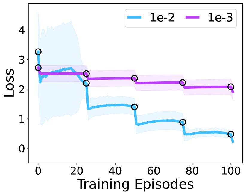
In Figure 5(b) we observe that there is no anticipation when we take only one gradient descent step on each document with learning rate 0.001. Here we experiment with one-step gradient descent using a higher learning rate, 0.01. We plot the resulting average loss curves under the same training setup in Figure 13. We observe that, with a larger learning rate, slight anticipation is still observed for $1$ gradient step.

B.3 Effect of Number of Attention Heads

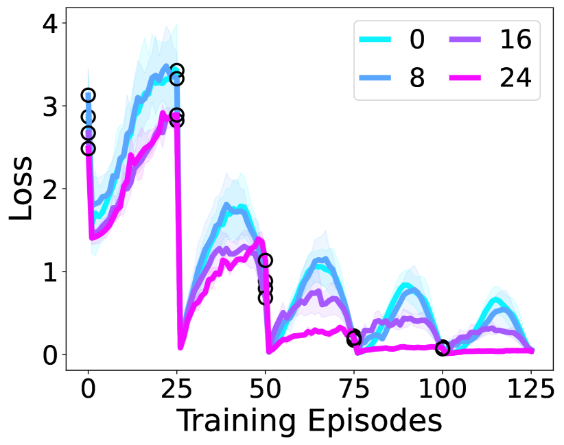
In addition to varying the model width and model depth in Figure 4, we also experimented with varying the number of attention heads $h\in\{2,4,8,16\}$ while keeping model width to be 2048 and model depth to be 16. Loss curves on document $\bm{x}_{1}$ are shown in figure 14. The results suggest that the number of attention heads does not have a big effect on cyclic training in our setting.

B.4 Effect of LLM Model Initialization

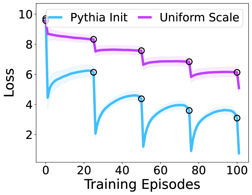
Here we compare the performance of the initialization scheme used by Biderman et al. (2023) (also used for all randomly initialized models in the main text) and a simple initialization scheme that samples the weight matrices from an isotropic Gaussian distribution with $\sigma=0.02$. The loss curves for document 1 under these two initializations of the Pythia-1B model are plotted in Figure 15. We observe that Pythia’s initialization scheme achieves much better average loss and also exhibits stronger anticipatory recovery. This demonstrates the importance of LLM initializations. The result is consistent with our observations in section 3.3 that the model’s ability to fit on each task is correlated with the amount of anticipatory recovery.

(a) Number of Gradient Steps with Inverse LR Scaling

(b) Number of Gradient Steps for Context Length 1024

Figure 16: Effect of number of gradient steps (a) with inverse learning rate scaling and (b) for context length 1024.

B.5 Effect of Number of Gradient Steps with Inverse Learning Rate Scaling

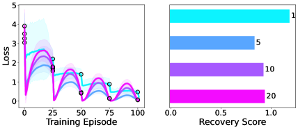
In Figure 16(a) we experiment with inversely scaling the learning rate with the number of gradient steps. We use a learning rate of $0.01$ for $M=1$, learning rate $0.002$ for $M=5$, learning rate $0.001$ for $M=10$, and learning rate $0.0005$ for $M=20$. The results suggest that the anticipation effect is stronger when the same total update is divided among more gradient steps.

B.6 Effect of Number of Gradient Steps for Long Context Length

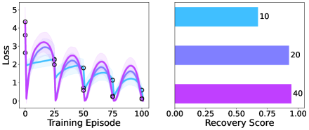
In Figure 16(b) we experiment with different number of gradient steps $M\in\{10,20,40\}$ for context length 1024. The results confirm that longer context length is not a fundamental limitation to anticipatory recovery, and we can achieve the same recovery score as a smaller context length with more gradient steps.

Appendix C Additional Visualizations

(a) Model Activations

(b) Model Weights

Figure 17: Magnitude of (a) model activation updates and (b) model weight updates through four epochs of cyclic training.

(a) 50 Documents

(b) 100 Documents

(c) 200 Documents

Figure 18: Loss recoveries for training on task $\bm{x}_{i}$ (y-axis) and evaluating on task $\bm{x}_{j}$ (x-axis) for longer document sequences of different lengths.

C.1 Magnitude of Changes in Model Weights and Model Activations

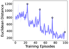
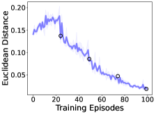
We plot the magnitude of the difference between the $\bm{x}_{1}$ activations of model checkpoints saved at consecutive episodes throughout four epochs of cyclic training of a Pythia-410M model in Figure 17(a), and observe a clear stepwise pattern. In contrast, the magnitude of model weight updates (Figure 17(b)) decreases monotonically over the training episodes and do not exhibit this stepwise pattern. This result is consistent with the pattern we observe in section 4.3.

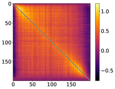
C.2 Pairwise Recovery Matrices for Longer Document Sequences

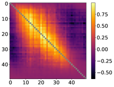
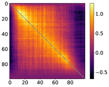
Similar to Figure 8(b), we plot the pairwise loss recoveries for each pair of documents $(\bm{x}_{i},\bm{x}_{j})$ in longer document sequences, where $T=50,100,200$ respectively, in Figure 18. We use the 1B model and default hyperparameters. We observe that, as we increase the length of the document sequence, the highlight area near the center of the matrix is separated into two blobs, one in the top-left corner and the other in the bottom-right corner. We also observe a ”boundary” on the sides of the matrix where there is little or no recovery. The width of this ”boundary” stays relatively constant across different lengths of document sequences and is around 10 to 15 documents. This confirms our observation in the main text that the recovery on document $\bm{x}_{j}$ when fine-tuning on a proximal document $\bm{x}_{i}$ is highest when the model checkpoint is taken from document $\bm{x}_{j\pm b}$ where $b$ is a small number relative to the length of the document sequence.

References

- Devlin et al. (2019) Jacob Devlin, Ming-Wei Chang, Kenton Lee, and Kristina Toutanova. BERT: Pre-training of deep bidirectional transformers for language understanding. In Conference of the North American Chapter of the Association for Computational Linguistics: Human Language Technologies, 2019.
- Brown et al. (2020) Tom Brown, Benjamin Mann, Nick Ryder, Melanie Subbiah, Jared D Kaplan, Prafulla Dhariwal, Arvind Neelakantan, Pranav Shyam, Girish Sastry, Amanda Askell, et al. Language models are few-shot learners. Advances in Neural Information Processing Systems, 33:1877–1901, 2020.
- Touvron et al. (2023) Hugo Touvron, Thibaut Lavril, Gautier Izacard, Xavier Martinet, Marie-Anne Lachaux, Timothée Lacroix, Baptiste Rozière, Naman Goyal, Eric Hambro, Faisal Azhar, et al. LLaMA: Open and efficient foundation language models. arXiv preprint arXiv:2302.13971, 2023.
- OpenAI (2023) OpenAI. Gpt-4 technical report, 2023.
- Hoffmann et al. (2022) Jordan Hoffmann, Sebastian Borgeaud, Arthur Mensch, Elena Buchatskaya, Trevor Cai, Eliza Rutherford, Diego de Las Casas, Lisa Anne Hendricks, Johannes Welbl, Aidan Clark, et al. Training compute-optimal large language models. arXiv preprint arXiv:2203.15556, 2022.
- Chowdhery et al. (2023) Aakanksha Chowdhery, Sharan Narang, Jacob Devlin, Maarten Bosma, Gaurav Mishra, Adam Roberts, Paul Barham, Hyung Won Chung, Charles Sutton, Sebastian Gehrmann, et al. PaLM: Scaling language modeling with pathways. Journal of Machine Learning Research, 24(240):1–113, 2023.
- Xue et al. (2024) Fuzhao Xue, Yao Fu, Wangchunshu Zhou, Zangwei Zheng, and Yang You. To repeat or not to repeat: Insights from scaling llm under token-crisis. Advances in Neural Information Processing Systems, 36, 2024.
- McCloskey and Cohen (1989) Michael McCloskey and Neal J Cohen. Catastrophic interference in connectionist networks: The sequential learning problem. In Psychology of Learning and Motivation, volume 24, pages 109–165. Elsevier, 1989.
- Biderman et al. (2023) Stella Biderman, Hailey Schoelkopf, Quentin Gregory Anthony, Herbie Bradley, Kyle O’Brien, Eric Hallahan, Mohammad Aflah Khan, Shivanshu Purohit, USVSN Sai Prashanth, Edward Raff, et al. Pythia: A suite for analyzing large language models across training and scaling. In International Conference on Machine Learning, pages 2397–2430. PMLR, 2023.
- Gao et al. (2020) Leo Gao, Stella Biderman, Sid Black, Laurence Golding, Travis Hoppe, Charles Foster, Jason Phang, Horace He, Anish Thite, Noa Nabeshima, et al. The Pile: An 800gb dataset of diverse text for language modeling. arXiv preprint arXiv:2101.00027, 2020.
- Biderman et al. (2022) Stella Biderman, Kieran Bicheno, and Leo Gao. Datasheet for the Pile. arXiv preprint arXiv:2201.07311, 2022.
- Nallapati et al. (2016) Ramesh Nallapati, Bowen Zhou, Cicero dos Santos, Çağlar Gulçehre, and Bing Xiang. Abstractive text summarization using sequence-to-sequence rnns and beyond. In Proceedings of the 20th SIGNLL Conference on Computational Natural Language Learning, pages 280–290, 2016.
- Kingma and Ba (2015) Diederik P. Kingma and Jimmy Ba. Adam: A method for stochastic optimization. In International Conference on Learning Representations, 2015.
- Chen et al. (2020) Mark Chen, Alec Radford, Rewon Child, Jeffrey Wu, Heewoo Jun, David Luan, and Ilya Sutskever. Generative pretraining from pixels. In International Conference on Machine Learning, pages 1691–1703. PMLR, 2020.
- Krizhevsky et al. (2009) Alex Krizhevsky, Geoffrey Hinton, et al. Learning multiple layers of features from tiny images. 2009.
- Dosovitskiy et al. (2020) Alexey Dosovitskiy, Lucas Beyer, Alexander Kolesnikov, Dirk Weissenborn, Xiaohua Zhai, Thomas Unterthiner, Mostafa Dehghani, Matthias Minderer, Georg Heigold, Sylvain Gelly, et al. An image is worth 16x16 words: Transformers for image recognition at scale. In International Conference on Learning Representations, 2020.
- Simonyan and Zisserman (2015) Karen Simonyan and Andrew Zisserman. Very deep convolutional networks for large-scale image recognition. In International Conference on Learning Representations, 2015.
- Deng et al. (2009) Jia Deng, Wei Dong, Richard Socher, Li-Jia Li, Kai Li, and Li Fei-Fei. Imagenet: A large-scale hierarchical image database. In 2009 IEEE conference on Computer Vision and Pattern Recognition, pages 248–255. IEEE, 2009.
- Ahn et al. (2020) Kwangjun Ahn, Chulhee Yun, and Suvrit Sra. SGD with shuffling: Optimal rates without component convexity and large epoch requirements. Advances in Neural Information Processing Systems, 33:17526–17535, 2020.
- Gurbuzbalaban et al. (2019) M Gurbuzbalaban, Asu Ozdaglar, and Pablo A Parrilo. Convergence rate of incremental gradient and incremental newton methods. SIAM Journal on Optimization, 29(4):2542–2565, 2019.
- Mishchenko et al. (2020) Konstantin Mishchenko, Ahmed Khaled, and Peter Richtárik. Random reshuffling: Simple analysis with vast improvements. Advances in Neural Information Processing Systems, 33:17309–17320, 2020.
- Safran and Shamir (2020) Itay Safran and Ohad Shamir. How good is SGD with random shuffling? In Conference on Learning Theory, pages 3250–3284. PMLR, 2020.
- Xu et al. (2022) Lijie Xu, Shuang Qiu, Binhang Yuan, Jiawei Jiang, Cedric Renggli, Shaoduo Gan, Kaan Kara, Guoliang Li, Ji Liu, Wentao Wu, et al. Stochastic gradient descent without full data shuffle. arXiv preprint arXiv:2206.05830, 2022.
- Jones et al. (2023) Matt Jones, Tyler R Scott, Mengye Ren, Gamaleldin ElSayed, Katherine Hermann, David Mayo, and Michael Mozer. Learning in temporally structured environments. 2023.
- Hannan (1957) James Hannan. Approximation to Bayes risk in repeated play. Contributions to the Theory of Games, 3:97–139, 1957.
- Zinkevich (2003) Martin Zinkevich. Online convex programming and generalized infinitesimal gradient ascent. In International Conference on Machine Learning, pages 928–936, 2003.
- Cesa-Bianchi and Lugosi (2006) Nicolo Cesa-Bianchi and Gábor Lugosi. Prediction, learning, and games. Cambridge University Press, 2006.
- Shalev-Shwartz et al. (2012) Shai Shalev-Shwartz et al. Online learning and online convex optimization. Foundations and Trends® in Machine Learning, 4(2):107–194, 2012.
- Denevi et al. (2019a) Giulia Denevi, Carlo Ciliberto, Riccardo Grazzi, and Massimiliano Pontil. Learning-to-learn stochastic gradient descent with biased regularization. In International Conference on Machine Learning, pages 1566–1575. PMLR, 2019a.
- Finn et al. (2019) Chelsea Finn, Aravind Rajeswaran, Sham Kakade, and Sergey Levine. Online meta-learning. In International Conference on Machine Learning, pages 1920–1930. PMLR, 2019.
- Denevi et al. (2019b) Giulia Denevi, Dimitris Stamos, Carlo Ciliberto, and Massimiliano Pontil. Online-within-online meta-learning. Advances in Neural Information Processing Systems, 32, 2019b.
- Javed and White (2019) Khurram Javed and Martha White. Meta-learning representations for continual learning. Advances in Neural Information Processing Systems, 32, 2019.
- Fini et al. (2020) Enrico Fini, Stéphane Lathuiliere, Enver Sangineto, Moin Nabi, and Elisa Ricci. Online continual learning under extreme memory constraints. In Proceedings of the European Conference on Computer Vision, pages 720–735. Springer, 2020.
- Ren et al. (2021) Mengye Ren, Michael Louis Iuzzolino, Michael Curtis Mozer, and Richard S. Zemel. Wandering within a world: Online contextualized few-shot learning. In International Conference on Learning Representations, 2021.
- Wang et al. (2021) Jianren Wang, Xin Wang, Yue Shang-Guan, and Abhinav Gupta. Wanderlust: Online continual object detection in the real world. In Proceedings of the IEEE/CVF International Conference on Computer Vision, pages 10829–10838, 2021.
- Biehl and Schwarze (1995) Michael Biehl and Holm Schwarze. Learning by on-line gradient descent. Journal of Physics A: Mathematical and general, 28(3):643, 1995.
- Vaswani et al. (2017) Ashish Vaswani, Noam Shazeer, Niki Parmar, Jakob Uszkoreit, Llion Jones, Aidan N Gomez, Łukasz Kaiser, and Illia Polosukhin. Attention is all you need. Advances in Neural Information Processing Systems, 30, 2017.
- Wei et al. (2022a) Jason Wei, Yi Tay, Rishi Bommasani, Colin Raffel, Barret Zoph, Sebastian Borgeaud, Dani Yogatama, Maarten Bosma, Denny Zhou, Donald Metzler, et al. Emergent abilities of large language models. Transactions on Machine Learning Research, 2022a.
- Wei et al. (2022b) Jason Wei, Xuezhi Wang, Dale Schuurmans, Maarten Bosma, Fei Xia, Ed Chi, Quoc V Le, Denny Zhou, et al. Chain-of-thought prompting elicits reasoning in large language models. Advances in Neural Information Processing Systems, 35:24824–24837, 2022b.
- Ganguli et al. (2022) Deep Ganguli, Danny Hernandez, Liane Lovitt, Amanda Askell, Yuntao Bai, Anna Chen, Tom Conerly, Nova Dassarma, Dawn Drain, Nelson Elhage, et al. Predictability and surprise in large generative models. In Proceedings of the 2022 ACM Conference on Fairness, Accountability, and Transparency, pages 1747–1764, 2022.
- Srivastava et al. (2022) Aarohi Srivastava, Abhinav Rastogi, Abhishek Rao, Abu Awal Md Shoeb, Abubakar Abid, Adam Fisch, Adam R Brown, Adam Santoro, Aditya Gupta, Adrià Garriga-Alonso, et al. Beyond the imitation game: Quantifying and extrapolating the capabilities of language models. arXiv preprint arXiv:2206.04615, 2022.
- Carlini et al. (2023) Nicholas Carlini, Daphne Ippolito, Matthew Jagielski, Katherine Lee, Florian Tramèr, and Chiyuan Zhang. Quantifying memorization across neural language models. In International Conference on Learning Representations, 2023.
- Orhan (2023) A Emin Orhan. Recognition, recall, and retention of few-shot memories in large language models. arXiv preprint arXiv:2303.17557, 2023.
- Van de Ven et al. (2020) Gido M Van de Ven, Hava T Siegelmann, and Andreas S Tolias. Brain-inspired replay for continual learning with artificial neural networks. Nature Communications, 11(1):4069, 2020.
- Kirkpatrick et al. (2017) James Kirkpatrick, Razvan Pascanu, Neil Rabinowitz, Joel Veness, Guillaume Desjardins, Andrei A Rusu, Kieran Milan, John Quan, Tiago Ramalho, Agnieszka Grabska-Barwinska, et al. Overcoming catastrophic forgetting in neural networks. Proceedings of the National Academy of Sciences, 114(13):3521–3526, 2017.
- Zenke et al. (2017) Friedemann Zenke, Ben Poole, and Surya Ganguli. Continual learning through synaptic intelligence. In International Conference on Machine Learning, pages 3987–3995. PMLR, 2017.
- Aljundi et al. (2018) Rahaf Aljundi, Francesca Babiloni, Mohamed Elhoseiny, Marcus Rohrbach, and Tinne Tuytelaars. Memory aware synapses: Learning what (not) to forget. In Proceedings of the European Conference on Computer Vision, pages 139–154, 2018.
- Rebuffi et al. (2017) Sylvestre-Alvise Rebuffi, Alexander Kolesnikov, Georg Sperl, and Christoph H Lampert. iCaRL: Incremental classifier and representation learning. In Proceedings of the IEEE conference on Computer Vision and Pattern Recognition, pages 2001–2010, 2017.
- Rolnick et al. (2019) David Rolnick, Arun Ahuja, Jonathan Schwarz, Timothy Lillicrap, and Gregory Wayne. Experience replay for continual learning. Advances in Neural Information Processing Systems, 32, 2019.
- Chaudhry et al. (2019) Arslan Chaudhry, Marcus Rohrbach, Mohamed Elhoseiny, Thalaiyasingam Ajanthan, Puneet K Dokania, Philip HS Torr, and Marc’Aurelio Ranzato. On tiny episodic memories in continual learning. arXiv preprint arXiv:1902.10486, 2019.
- Hinton et al. (2015) Geoffrey Hinton, Oriol Vinyals, and Jeff Dean. Distilling the knowledge in a neural network. arXiv preprint arXiv:1503.02531, 2015.
- Li and Hoiem (2017) Zhizhong Li and Derek Hoiem. Learning without forgetting. IEEE Transactions on Pattern Analysis and Machine Intelligence, 40(12):2935–2947, 2017.
- Buzzega et al. (2020) Pietro Buzzega, Matteo Boschini, Angelo Porrello, Davide Abati, and Simone Calderara. Dark experience for general continual learning: a strong, simple baseline. Advances in Neural Information Processing Systems, 33:15920–15930, 2020.
- Madaan et al. (2023) Divyam Madaan, Hongxu Yin, Wonmin Byeon, Jan Kautz, and Pavlo Molchanov. Heterogeneous continual learning. In Proceedings of the IEEE/CVF Conference on Computer Vision and Pattern Recognition, pages 15985–15995, 2023.
- Yoon et al. (2018) Jaehong Yoon, Eunho Yang, Jeongtae Lee, and Sung Ju Hwang. Lifelong learning with dynamically expandable networks. In International Conference on Learning Representations, 2018.
- Serra et al. (2018) Joan Serra, Didac Suris, Marius Miron, and Alexandros Karatzoglou. Overcoming catastrophic forgetting with hard attention to the task. In International Conference on Machine Learning, pages 4548–4557. PMLR, 2018.
- Gurbuz and Dovrolis (2022) Mustafa B Gurbuz and Constantine Dovrolis. NISPA: Neuro-inspired stability-plasticity adaptation for continual learning in sparse networks. In International Conference on Machine Learning, pages 8157–8174. PMLR, 2022.
- Kang et al. (2022) Haeyong Kang, Rusty John Lloyd Mina, Sultan Rizky Hikmawan Madjid, Jaehong Yoon, Mark Hasegawa-Johnson, Sung Ju Hwang, and Chang D Yoo. Forget-free continual learning with winning subnetworks. In International Conference on Machine Learning, pages 10734–10750. PMLR, 2022.
- Davidson and Mozer (2020) Guy Davidson and Michael C Mozer. Sequential mastery of multiple visual tasks: Networks naturally learn to learn and forget to forget. In Proceedings of the IEEE/CVF conference on Computer Vision and Pattern Recognition, pages 9282–9293, 2020.
- Janson et al. (2022) Paul Janson, Wenxuan Zhang, Rahaf Aljundi, and Mohamed Elhoseiny. A simple baseline that questions the use of pretrained-models in continual learning. In NeurIPS 2022 Workshop on Distribution Shifts: Connecting Methods and Applications, 2022.
- Lee et al. (2023) Kuan-Ying Lee, Yuanyi Zhong, and Yu-Xiong Wang. Do pre-trained models benefit equally in continual learning? In Proceedings of the IEEE/CVF Winter Conference on Applications of Computer Vision, pages 6485–6493, 2023.
- Fini et al. (2022) Enrico Fini, Victor G Turrisi Da Costa, Xavier Alameda-Pineda, Elisa Ricci, Karteek Alahari, and Julien Mairal. Self-supervised models are continual learners. In Proceedings of the IEEE/CVF Conference on Computer Vision and Pattern Recognition, pages 9621–9630, 2022.
- Scialom et al. (2022) Thomas Scialom, Tuhin Chakrabarty, and Smaranda Muresan. Fine-tuned language models are continual learners. In Proceedings of the 2022 Conference on Empirical Methods in Natural Language Processing, pages 6107–6122, 2022.
- Ke et al. (2022) Zixuan Ke, Yijia Shao, Haowei Lin, Tatsuya Konishi, Gyuhak Kim, and Bing Liu. Continual pre-training of language models. In International Conference on Learning Representations, 2022.
- Mayo et al. (2023) David Mayo, Tyler Scott, Mengye Ren, Gamaleldin Elsayed, Katherine Hermann, Matt Jones, and Michael Mozer. Multitask learning via interleaving: A neural network investigation. In M. Goldwater, F. K. Anggoro, B. K. Hayes, and D. C. Ong, editors, Proceedings of the 45th Annual Conference of the Cognitive Science Society, volume 45, 2023.