Self-Consistency Training for Hamiltonian Prediction
Abstract
Hamiltonian prediction is a versatile formulation to leverage machine learning for solving molecular science problems. Yet, its applicability is limited by insufficient labeled data for training. In this work, we highlight that Hamiltonian prediction possesses a self-consistency principle, based on which we propose an exact training method that does not require labeled data. This merit addresses the data scarcity difficulty, and distinguishes the task from other property prediction formulations with unique benefits: (1) self-consistency training enables the model to be trained on a large amount of unlabeled data, hence substantially enhances generalization; (2) self-consistency training is more efficient than labeling data with DFT for supervised training, since it is an amortization of DFT calculation over a set of molecular structures. We empirically demonstrate the better generalization in data-scarce and out-of-distribution scenarios, and the better efficiency from the amortization. These benefits push forward the applicability of Hamiltonian prediction to an ever larger scale.
1 Introduction
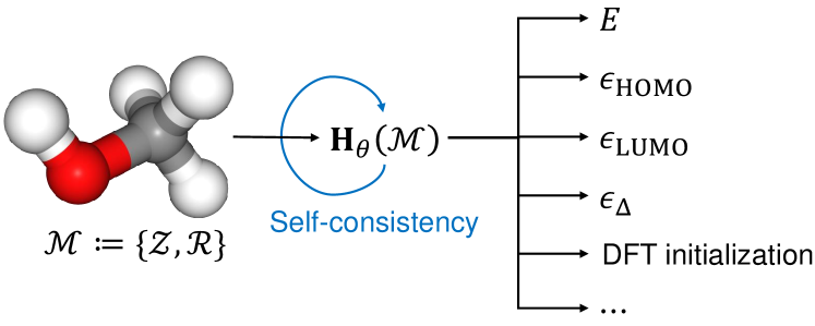
Calculating properties of molecules is the foundation for a wide range of industry needs including drug design, protein engineering, and material discovery. The key to these properties is the quantum mechanics effect of electrons in the molecule, for which various quantum chemistry methods are proposed. Density functional theory (DFT) (Hohenberg & Kohn, 1964; Kohn & Sham, 1965; Perdew et al., 1996; Teale et al., 2022) is perhaps the most prevailing choice due to its balanced accuracy and efficiency, but still hard to meet the demand in industry. Encouraged by the impressive advancement in machine learning, researchers have trained machine learning models on datasets with property labels to directly predict properties of queried molecules (Ramakrishnan et al., 2014; Chmiela et al., 2019; Chanussot et al., 2021). For each property, a separate model (at least a separate output module) needs to be trained. A more fundamental formulation is to predict the Hamiltonian matrix (Schütt et al., 2019) (more precisely, the Fock matrix in a DFT calculation when the self-consistent field (SCF) iteration converges). The Hamiltonian matrix can directly provide all the properties that a DFT calculation can (Fig. 1), waiving the need to specify the target property or train multiple models. Moreover, Hamiltonian prediction can also accelerate running DFT by providing an accurate initialization.
Noticeable progress has been made for Hamiltonian prediction. Hegde & Bowen (2017) pioneered the direction using kernel ridge regression to predict semi-empirical Hamiltonian for one-dimensional systems. Schütt et al. (2019) then proposed a neural network model called SchNorb to predict Hamiltonian for small molecules, which is further enhanced for prediction efficiency by Gastegger et al. (2020). Shmilovich et al. (2022) proposed to employ atomic orbital features for Hamiltonian prediction. Noting that the Hamiltonian matrix is composed of tensors in various orders which are equivariant to coordinate rotation in respective ways, subsequent works proposed neural network model architectures that guarantee the equivariance. Some works (Unke et al., 2021; Yu et al., 2023b; Gong et al., 2023; Yin et al., 2024) include high-order tensorial features into model input, which are processed in an equivariant way typically with tensor products. Li et al. (2022) used local frames to anchor coordinate systems with the molecule so that the prediction target is invariant. Zhang et al. (2022); Nigam et al. (2022) implemented the prediction by constructing equivariant kernels. There are works that exploited data other than the Hamiltonian directly, e.g., using orbital energies (Wang et al., 2021b; Gu et al., 2022; Zhong et al., 2023) to supervise the prediction of Hamiltonian. While these prior efforts have introduced powerful architectures showing encouraging outcomes, they all rely on datasets providing Hamiltonian or orbital energy labels. Since such datasets are scarce, the applicability of Hamiltonian prediction is restricted to molecules with no more than 31 atoms (Yu et al., 2023a).111 There are a few works (Li et al., 2022; Gong et al., 2023) that have demonstrated applicability to large-scale material systems. We note that this is achieved by leveraging the periodicity and locality in material systems, which do not hold perfectly in molecular systems.
In this work, we highlight a uniqueness of Hamiltonian prediction: it has a self-consistency principle (indicated by the blue loop arrow in Fig. 1), by leveraging which we design a training method that guides the model without labeled data. The self-consistency originates from the basic equation of DFT (Eq. (2)) that the Hamiltonian needs to satisfy. Conventional DFT solves the equation using a fixed-point iteration process called self-consistent field (SCF) iteration. In contrast, the proposed self-consistency training solves the equation by directly minimizing the residue of the equation incurred by the model-predicted Hamiltonian (Fig. 2). As the equation fully determines the prediction target, no Hamiltonian label is required, and the loss function is minimized only if the equation is satisfied and the prediction is exact. Self-consistency training compensates data scarcity with physical laws, and differentiates Hamiltonian prediction from other machine learning formulations (e.g., energy prediction), in that it enables continued self-improvement without additional labeled data.
We exploit the merit of self-consistency training in two specific points. (1) Self-consistency training leverages unlabeled data, which allows substantial improvement of the generalizability of the Hamiltonian prediction model. We demonstrate that the predicted Hamiltonian as well as derived molecular properties are indeed improved by a significant margin, when labeled data is limited (data-scarce scenario) and when the model is evaluated on molecules larger than those used in training (out-of-distribution scenario).
(2) Self-consistency training on unlabeled data is more efficient than generating labels using DFT on those data for supervised learning, as we find that self-consistency training can be seen as an amortization of DFT calculation over a set of molecules. DFT requires multiple SCF iterations on each molecule before providing supervision, while self-consistency training only costs equivalently one SCF iteration to return a training signal, hence provides information on more molecules given the same amount of computation. The better efficiency for Hamiltonian prediction training is empirically verified in both data-scarce and out-of-distribution scenarios. More attractively, even given sufficient computational budget, supervised learning with all additional labels still exhibits larger error in derived molecular properties, indicating that self-consistency training is more relevant to physical quantities. We also verified the better efficiency to solve a bunch of molecules using self-consistency training than using DFT.
Finally, we demonstrate that with the above two unique benefits of self-consistency training, the applicability of Hamiltonian prediction can overcome the data limit and is extended to molecules much larger (56 atoms) than previously supported, showing increased practical relevance. It also derives orders better molecular property results on these large molecules than end-to-end property prediction models, which are limited by available labeled data.
2 Self-Consistency Training
2.1 Preliminaries
We first provide a schematic description of the calculation mechanism of DFT and conventional supervised learning for Hamiltonian prediction before delving into self-consistency training. Appendix A provides more details.
For a given molecular structure , where and specifies the atomic numbers (types) and coordinates of the nuclei in the molecule, DFT solves the ground state of the electrons in the molecule by minimizing electronic energy under a reduced representation of electronic state, which is one-electron wavefunctions, called orbitals. Here, represents the Cartesian coordinates of an electron. For practical calculation, a basis set of functions on is used to expand the orbitals. To roughly align with the electronic structure, the basis functions depend on the molecular structure, hence are denoted as . Expansion coefficients of the orbitals are collected into a matrix in the following way: .
DFT typically solves the electronic energy minimization problem w.r.t by directly solving the optimality equation:
| (2) |
which is called the Kohn-Sham equation. Here, is a matrix-valued function with an explicit expression (Appendix A.5). This matrix is called the Hamiltonian matrix (also noted as the Fock matrix) due to the resemblance of the equation to the Schrödinger equation. The matrix is the overlap matrix of the basis, which can be computed analytically for common basis choices. Eq. (2) can be seen as a generalized eigenvalue problem defined by the matrices and . Under this view, the coefficients of orbitals in the equation can be understood as eigenvectors, and the diagonal matrix comprises eigenvalues which are referred to as orbital energies.
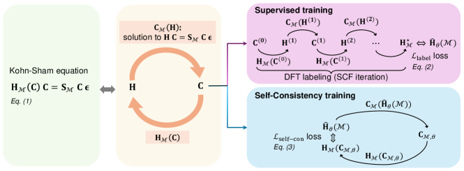
However, the difficulty to solve Eq. (2) is that, the matrix that defines the problem and the eigenvector solution are intertwined: the eigenvectors need to recover the Hamiltonian matrix that defined the eigenvalue problem through the explicit function (Fig. 2, middle). Conventional DFT calculation solves it using a fixed-point iteration process called self-consistent field (SCF) iteration. In each step, orbital coefficients are used to construct the Hamiltonian matrix , which defines a generalized eigenvalue problem , whose eigenvectors, denoted as , are taken as the updated orbital coefficients (Fig. 2, top right). The converged Hamiltonian and its eigenvectors hence solve Eq. (2), which then derive various molecular structures.
Hamiltonian prediction aims to bypass the SCF iteration by directly predicting from molecular structure using a machine-learning model ,222The “hat” or “circumflex” accent in the notation here is meant to represent “a neural-network estimator” (but not an operator as the convention in quantum mechanics). where denotes the model parameters to be learned. The conventional way to learn such a model is by supervised learning, which requires running DFT on a set of molecular structures to construct a labeled dataset , on which the supervised training loss function is applied:
| (3) |
where denotes the number of samples in the set . The squared Frobenius norm amounts to the mean squared error (MSE) over the matrix entries. Some works (Unke et al., 2021; Yu et al., 2023b) also include a mean absolute error (MAE) loss for more efficient learning.
2.2 Self-Consistency Training
We now describe the proposed self-consistency training for Hamiltonian prediction. It can be seen as another way to solve the Kohn-Sham equation (2), which the prediction needs to satisfy. Recall that the equation is equivalent to the condition that , i.e., the eigenvectors of the generalized eigenvalue problem defined by the Hamiltonian matrix , construct the same Hamiltonian matrix, i.e., (Fig. 2, middle). The self-consistency training loss is hence designed to enforce this condition: the difference between the predicted Hamiltonian and the reconstructed Hamiltonian from itself should be minimized, where the reconstruction is done by first solving for the eigenvectors of the generalized eigenvalue problem defined by then constructing the Hamiltonian using (Fig. 2, bottom right). Explicitly, the self-consistency loss is:
| (4) |
Following the practice of prior work (Unke et al., 2021; Yu et al., 2023b), we also include its MAE counterpart in place of the squared Frobenius norm into the loss. The implementation process is summarized in Alg. 1. Note that the loss only requires a set of molecular structures unnecessarily with Hamiltonian labels. It thus enables leveraging numerous molecular structures for learning Hamiltonian prediction, which could substantially enhance generalizability of the prediction model to a wide range of molecules, allowing applicability beyond the limitation of labeled datasets.
We remark that the self-consistency loss is distinct from regularization or self-supervised training, in the sense that the loss by itself can already drive the model towards the exact target, since the loss enforces the equation that determines the target. We also emphasize that the loss should not be interpreted as updating the prediction towards the reconstructed Hamiltonian as a fixed target (which is the case when the stop_grad operation is applied), and the back-propagation (i.e., computation of the gradient of the loss w.r.t ) through the Hamiltonian reconstruction process is indispensable. This is because the reconstructed Hamiltonian unnecessarily comes closer to the target solution (Cances & Le Bris, 2000; Pulay, 1982), so taking the reconstructed Hamiltonian as a constant when optimizing may even make the model worse. Instead, the loss aims to minimize the change from the reconstruction process. To minimize this change, both the predicted matrix and the reconstructed matrix are driven towards the solution.
2.3 Implementation Considerations
For stable and efficient optimization of the self-consistency loss, we mention a few technical treatments.
Back-Propagation through Eigensolver.
As mentioned, back-propagation through the reconstruction process is indispensable. This requires differentiation calculation through the eigensolver . We leverage the eigensolver implemented in an automatic differentiation package PyTorch (Paszke et al., 2019) which automatically provides the differentiation calculation. Nevertheless, the calculation often appears numerically unstable (Ionescu et al., 2015; Wang et al., 2019), as it relies on a matrix (see Appendix B.2 for detailed derivation),
| (5) |
where is -th eigenvalue. When there are two close eigenvalues, the values in can be exceedingly large, causing unstable training. To mitigate this instability, we introduce two treatments. The first is simply truncating the values in if they are larger than a chosen threshold. The second treatment is to skip the model parameter update when the scale of the gradient w.r.t parameters exceeds a certain threshold. Appendix B.2 presents more details.
Efficient Hamiltonian Reconstruction.
Evaluating the function is also a costly procedure, mainly due to two computational components. The first is the evaluation of basis functions on a quadrature grid for evaluating the exchange-correlation component of the Hamiltonian matrix (Appendix A.5). To accelerate this part, we implemented a GPU-based evaluation process of basis functions on grid points. The other costly procedure is the evaluation of the Hartree component of the Hamiltonian matrix, which requires cost in its vanilla form. For efficient evaluation of this term, we adopt the density fitting approach (Appendix A.5), a widely used technique in DFT to reduce the complexity to with acceptable loss of accuracy.
| Molecule | Setting | SCF Accel. | ||||||
|---|---|---|---|---|---|---|---|---|
| Ethanol | label | 160.36 | 712.54 | 99.44 | 911.64 | 6800.84 | 6643.11 | 68.3 |
| label + self-con | 75.65 | 285.49 | 99.94 | 336.97 | 1203.60 | 1224.86 | 61.5 | |
| Malondi- | label | 101.19 | 456.75 | 99.09 | 471.92 | 1093.22 | 1115.94 | 69.1 |
| aldehyde | label + self-con | 86.60 | 280.39 | 99.67 | 274.45 | 279.14 | 324.37 | 62.1 |
| Uracil | label | 88.26 | 1079.51 | 95.83 | 1217.17 | 12496.1 | 11850.56 | 65.8 |
| label + self-con | 63.82 | 315.40 | 99.58 | 359.98 | 369.67 | 388.30 | 54.5 |
2.4 Amortization of DFT Calculation
As mentioned in Sec. 2.2, self-consistency training can be applied to almost unlimited unlabeled molecular structures, hence could substantially improve the generalizability of a Hamiltonian prediction model. Here, we point out that self-consistency training is also more efficient to improve generalizability than generating additional labels using DFT on those data and then supervising the model. This is based on the interpretation that self-consistency training is an amortization of DFT calculation: for a given molecular structure , DFT requires multiple SCF iterations for convergence before it can provide a supervision on (Fig. 2, top right), while self-consistency training only requires one SCF iteration to evaluate the loss and guide the training on (Fig. 2, bottom right). This indicates that given the same amount of computational resources measured in the number of SCF iterations, self-consistency training can spread the resource on more molecular structures, hence providing information on a larger range of the input space. This is more valuable than Hamiltonian labels on fewer molecular structures for the model to generalize to a broad range of molecular structures.
As an alternative way to carry out DFT calculation, self-consistency training of a Hamiltonian prediction model can be more efficient to solve a large amount of molecular structures collectively than directly using conventional DFT calculation on them. Apart from the amortization effect of self-consistency training, the efficiency is also benefited from the generalization of a Hamiltonian prediction model to similar molecular structures, on which the model can already provide close results. The demand to solve a set of molecular structures is not uncommon; e.g., high-throughput drug screening requires investigating a large amount of ligand-receptor compounds using DFT (Jordaan et al., 2020). Therefore, the applicability scope of Hamiltonian prediction with self-consistency training is enlarged.
3 Experimental Results
| Setting | SCF Accel. | ||||||
|---|---|---|---|---|---|---|---|
| zero-shot | 69.67 | 403.52 | 95.72 | 778.86 | 12230.49 | 12203.12 | 66.3 |
| self-con (all-param) | 65.74 | 375.31 | 97.31 | 565.50 | 1130.55 | 1316.96 | 64.5 |
| self-con (adapter) | 64.48 | 268.83 | 97.12 | 449.80 | 1220.54 | 1394.29 | 65.0 |
| FT mode | Setting | SCF Accel. | ||||||
|---|---|---|---|---|---|---|---|---|
| All | extended-label | 62.13 | 365.66 | 96.89 | 577.46 | 5962.16 | 6137.66 | 65.0 |
| self-con | 65.74 | 375.31 | 97.31 | 565.50 | 1130.55 | 1316.96 | 64.5 | |
| Adapter | extended-label | 59.67 | 330.05 | 96.63 | 541.92 | 6372.12 | 6445.33 | 65.2 |
| self-con | 64.48 | 268.83 | 97.12 | 449.80 | 1220.54 | 1394.29 | 65.0 |
We now empirically validate the benefits of self-consistency training. We adopt QHNet (Yu et al., 2023b) as the Hamiltonian prediction model, which is an -equivariant graph neural network that balances efficiency and accuracy. We employ the following metrics to measure prediction accuracy. A direct metric is the mean absolute error (MAE) over matrix entries between the predicted and DFT-solved Hamiltonian matrices, as introduced by Schütt et al. (2019). Directly derived quantities from Hamiltonian, including orbital energies and coefficients solved from the generalized eigenvalue problem, are also used to assess accuracy, measured by MAE for and cosine similarity for . We also report the MAE for three molecular properties relevant to molecular research, including the HOMO and LUMO energies , and their gap , which can be computed from Hamiltonian. We also assess the utility for accelerating DFT by the ratio of the number of SCF steps until convergence when using the prediction as initialization over the number of SCF steps using standard initialization (denoted as SCF Accel.).
3.1 Self-Consistency Training Improves Generalization
As discussed in Sec. 2.2, self-consistency training can leverage unlabeled data to improve generalizability. We validate this benefit on two challenging generalization scenarios.
Data-Scarce Scenario.
For some scientific tasks with limited labels available (denoted as ), it is difficult for the machine learning model to achieve an admirable performance even for in-distribution (ID) generalization. To demonstrate the advantage of self-consistency training in this scenario, we conduct experiments on three conformational spaces from MD17 (Chmiela et al., 2019; Schütt et al., 2019), specifically focusing on ethanol, malondialdehyde and uracil molecules. The train/validation/test split setting used in (Schütt et al., 2019) is adopted. To simulate a data-scarce setting, only 100 training Hamiltonian labels for each conformational space are available for supervised training using the label loss (Eq. (3)). On the large amount of unlabeled structures in the training set (dubbed , about 24,900 structures), we apply the self-consistency loss (Eq. (4)) and jointly train it with the label loss. The resulting total loss function is expressed as:
| (6) |
where is a weighting factor. See more training details in Appendix C.4.
Prediction results on test structures are summarized in Table 1. Compared to the results of supervised (label-based) training, applying self-consistency loss on unlabeled structures leads to a substantial improvement across all evaluation metrics and molecules. Notably, it achieves a significant reduction in the Hamiltonian MAE, with decreases from 14.4% to 52.8%. Furthermore, the MAE for , and is lowered by several folds. These findings underscore the attractive capability of self-consistency training in boosting ID generalizability in the data-scarce scenario.
Out-of-Distribution (OOD) Scenario.
Yu et al. (2023a) introduced the QH9 dataset to benchmark Hamiltonian prediction over the chemical space. Their findings highlight a challenging out-of-distribution (OOD) generalization scenario: models trained on smaller molecules often struggle to generalize to larger molecules. To demonstrate the significance of generalizability of self-consistency training, we evaluate its performance on a similar OOD scenario. Following Yu et al. (2023a), we divide the molecular structures in QH9 into two subsets: QH9-small which comprises molecules with no more than 20 atoms, and QH9-large which includes those with more than 20 atoms. The two subsets are then correspondingly divided at random into distinct training/validation and training/validation/test splits (see more dataset details in Appendix C.1). To evaluate OOD generalization, we first train the model on the QH9-small subset using supervised loss , then fine-tune the model only using the self-consistency loss on unlabeled molecules from the QH9-large training split, and finally evaluate the model on QH9-large test molecules. The model only trained on the QH9-small subset is taken as baseline (dubbed zero-shot). For the fine-tuning phase, we consider two variants: fine-tuning all parameters of the model (all-param), or introducing an adapter module atop the model which is the only optimized component (adapter). We ensure all models are sufficiently trained. Appendix C.4 shows more training details.
As shown in Table 2, compared to the zero-shot generalization results, employing self-consistency training on unlabeled QH9-large molecules can substantially improve performance on test large molecules across two fine-tuning settings. Remarkably, self-consistency training reduces the MAE of and by an order of magnitude. These results verify the effectiveness of self-consistency training in improving OOD generalization.
3.2 Self-Consistency Training Amortizes DFT Calculation
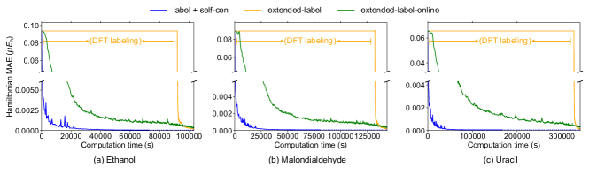
As discussed in Sec. 2.4, self-consistency training can improve model generalization more efficiently than DFT labeling since it acts as an amortization of DFT calculation. We validate this amortization effect by showing the accuracy-cost curves on the same two scenarios studied in Sec. 3.1. Specifically, the accuracy is measured using the validation Hamiltonian MAE during training, whereas the cost is measured by the cumulative computational time spent on training neural networks using GPU and generating DFT labels on CPU. All methods are implemented on a workstation equipped with an NVIDIA A100 GPU with 80 GiB memory and a 24-core AMD EPYC CPU.
Data-Scarce Scenario.
On unlabeled molecular structure data, self-consistency training dedicates all computation to optimizing the model, while supervised training allocates the computational budget firstly to generate extended labels on these structures using DFT and then optimize the model (dubbed extended-label). Accuracy-cost curves are presented in Fig. 3. We see that self-consistency training rapidly converges to a low prediction error at a relatively modest cost, while the extended-label setting incurs a significantly higher cost to reach a comparable accuracy level, due to the extensive resources required for DFT labeling. To enhance the performance of the extended-label setting in the low-cost region, we hence also consider an online training strategy (dubbed extended-label-online): each iteration involves generating labels for first-encountered structures, followed by supervising the model using the label loss. This setting provides supervision signals in every iteration, rather than labeling the entire training set upfront. Nevertheless, self-consistency training still outperforms the extended-label-online setting across a range of computational budget.
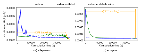
Out-of-Distribution (OOD) Scenario.
For the challenging OOD scenario, we still evaluate the model on QH9-large test molecules. All three training settings are implemented by fine-tuning the model that is initially pretrained on QH9-small molecules. The curves on QH9-large validation molecules are presented in Fig. 4. Self-consistency training can achieve a commendable generalization accuracy at a relatively low cost, across both fine-tuning settings. In contrast, the extended-label and extended-label-online settings require a significantly higher computational cost to reach comparable levels of accuracy. These results indicate the effective amortization effect of self-consistency training.
Notably, given adequate computational budget, supervised learning can extend sufficient labeled data to capture the whole data distribution. In such cases, it serves as an upper bound of Hamiltonian prediction performance for self-consistency training, as DFT labels can provide a more direct supervision signal to machine learning models than the self-consistency principle. Empirically, we also observe that, with adequate computation time(e.g., at the end of curves in Fig. 4), supervised training can outperform self-consistency training. Nevertheless, this superior performance in terms of Hamiltonian MAE does not consistently extend to molecular properties. As indicated in Table 3, while supervised training (extended-label) may achieve a marginally lower Hamiltonian MAE than self-consistency training on QH9-large test molecules, self-consistency training significantly outperforms both supervised training settings in predicting , and properties. A plausible explanation is that the self-consistency principle enforces the model to infer a solution more relevant to physical quantities. We also identify a similar trend in conformational spaces and detail the analysis in Appendix D.1.
Direct Evaluation of Amortization Effect.
To directly assess the amortization effect, we compare the computational cost of self-consistency training against DFT for solving a bunch of molecules, e.g., the unlabeled training structures in the data-scarce scenario. Specifically, we train the Hamiltonian prediction model using the combined loss (Eq. (6)) until convergence, and record the computational time as . Then we evaluate the MAE of electronic energy of the model prediction, and take the value as the convergence criterion (second column of Table 4) for running DFT on the same set of unlabeled structures, whose computational time is recorded as . As shown in Table 4, self-consistency training requires lower computational cost than DFT to reach the same level of accuracy, demonstrating the effective benefit of amortization. Appendix D.2 shows more implementation details.
| Molecule | criterion | ||
|---|---|---|---|
| Ethanol | 3.10 | 4.50 | 6.40 |
| Malondialdehyde | 8.89 | 4.81 | 1.05 |
| Uracil | 1.77 | 1.23 | 2.15 |
| Molecule | Setting | SCF Accel. | ||||||
|---|---|---|---|---|---|---|---|---|
| ALA3 | zero-shot | 237.71 | 6.54 | 52.24 | 6.90 | 9.51 | 9.79 | 84.6 |
| self-con | 52.49 | 1.22 | 94.46 | 2.07 | 3.76 | 2.69 | 64.7 | |
| e2e (ET) | N/A | N/A | N/A | 1.74 | 7.72 | 2.38 | N/A | |
| e2e (Equiformer) | N/A | N/A | N/A | 2.38 | 1.16 | 2.27 | N/A | |
| DHA | zero-shot | 397.87 | 1.84 | 20.15 | 1.11 | 1.90 | 1.85 | 170.8 |
| self-con | 56.12 | 1.81 | 83.51 | 1.99 | 4.01 | 2.34 | 67.0 | |
| e2e (ET) | N/A | N/A | N/A | 2.92 | 2.58 | 3.39 | N/A | |
| e2e (Equiformer) | N/A | N/A | N/A | 3.76 | 2.31 | 4.17 | N/A |
3.3 Self-Consistency Training Enables Applicability to Large-Scale Molecular Systems
To wield the advantage of self-consistency training for a larger impact, we study its generalization performance on molecules that are larger than all previously reported.
Large-Scale Generalization.
In practice, we consider two molecules in the MD22 dataset (Chmiela et al., 2023), Ac-Ala3-NHMe (ALA3, 42 atoms) and DHA (56 atoms). Both molecules exceed the size of the largest molecule in the QH9 dataset (31 atoms) with a significant gap. Due to the extensive DFT cost, we select a random subset of 500 structures from each molecule as the evaluation benchmark. For running on large molecules, we pretrain the model on nearly all QH9 molecules (the QH9-Full setting in Table C.2), then fine-tune the model using the self-consistency loss on the selected MD22 structures, and finally benchmark the model on the same MD22 structures. For ease of training, we employ the MINAO initialization (Sun et al., 2018) as a base Hamiltonian and let the model learn the residual correction, and adopt the all-param fine-tuning approach.
The results presented in Table 5 reveal a stark contrast between the zero-shot generalization performance on MD22 of the model (with Hamiltonian MAE of 237.71 for ALA3 and 397.87 for DHA) and its validation performance on QH9 (29.06). The significant performance drop is mainly attributable to the substantial scale gap between QH9 and MD22. Remarkably, applying the self-consistency loss on unlabeled structures achieves an impressive performance improvement, notably reducing the MAE of and by an order of magnitude. More importantly, when considering the acceleration benefit for SCF, zero-shot prediction only brings a limited acceleration gain (84.6% on ALA3) and even results in a deceleration (170.8% on DHA). In contrast, self-consistency training achieves impressive SCF acceleration ratios of 65.1% for ALA3 and 66.3% for DHA. These findings imply the potential of self-consistency training for practical usage.
Comparison with End-to-End Property Predictor.
For molecular property prediction, a conventional paradigm is to predict some specified property in an end-to-end (e2e) manner (Schütt et al., 2018; Gasteiger et al., 2020; Thölke & De Fabritiis, 2021; Liao & Smidt, 2022). Yet, Hamiltonian prediction methods offer a distinct advantage by providing all DFT-related properties using a single model. Furthermore, self-consistency training differentiates Hamiltonian prediction from other machine-learning prediction formulations, since it enables continued improvement of Hamiltonian prediction without labeled data, henceforth improving various molecular properties. To showcase this unique merit, we compare the properties derived from predicted Hamiltonian after self-consistency training, with e2e prediction of these properties, which cannot be further improved without additional labeled data. Specifically, we choose two advanced e2e architectures, ET (Thölke & De Fabritiis, 2021) and Equiformer (Liao & Smidt, 2022), as our baselines. The evaluation focuses on three important properties: , and . To ensure a fair comparison, we retrain the ET and Equiformer models on the QH9 dataset and study their generalization performance on MD22.
The results in Table 5 indicate that the Hamiltonian prediction model, when used in a zero-shot fashion, exhibits superior generalization on and , yet fall short on compared to the zero-short generalization of e2e baselines. Notably, when the self-consistency loss is incorporated, the Hamiltonian model significantly surpasses the two e2e baselines, reducing the prediction error by one or two orders of magnitude. These results indicate that self-consistency training offers a promising avenue for improving OOD property prediction in a data-free manner.
4 Conclusion
We have presented self-consistency training for Hamiltonian prediction, a novel training method that does not require labeled data. This is a unique advantage of Hamiltonian prediction. As the self-consistency loss is designed to enforce the basic equation of DFT, it provides complete and exact information of the prediction target. Self-consistency training opens the access to gain supervision from vastly available unlabeled data, which substantially solves the data-scarce problem and allows generalization to challenging domains. We have also pointed out and empirically verified that self-consistency training is more efficient than running DFT to generate data for supervised learning, benefited from its amortization effect. Using self-consistency training, we have pushed Hamiltonian prediction to solve molecules larger than ever reported.
More broadly, since Hamiltonian matrix can derive rich molecular properties (e.g., energy, HOMO-LUMO gap), the self-consistency training can also improve the prediction of these properties without labeled data, and can even supervise end-to-end prediction models. Since labeled data in the science domain in general is much less than in conventional AI domains, and generalization is more challenging due to the flexibility in the input, this way to leverage fundamental physical laws to train the model would be especially helpful.
Acknowledgements
We thank Lin Huang, Han Yang for insightful discussions; Erpai Luo for valuable discussions on model design and help with preparing datasets; Tao Qin, Jia Zhang and Huanhuan Xia for their constructive feedback. Additionally, we acknowledge Lin Huang, Han Yang, and Jia Zhang for providing their CuDA implementation for Hamiltonian construction.
References
- Becke (1992) Becke, A. D. Density-functional thermochemistry. I. the effect of the exchange-only gradient correction. The Journal of chemical physics, 96(3):2155–2160, 1992.
- Becke (1993) Becke, A. D. Density-functional thermochemistry. III. The role of exact exchange. The Journal of Chemical Physics, 98, 1993. ISSN 00219606. doi: 10.1063/1.464913.
- Cances & Le Bris (2000) Cances, E. and Le Bris, C. On the convergence of SCF algorithms for the Hartree-Fock equations. ESAIM: Mathematical Modelling and Numerical Analysis, 34(4):749–774, 2000.
- Chanussot et al. (2021) Chanussot, L., Das, A., Goyal, S., Lavril, T., Shuaibi, M., Riviere, M., Tran, K., Heras-Domingo, J., Ho, C., Hu, W., et al. Open catalyst 2020 (OC20) dataset and community challenges. Acs Catalysis, 11(10):6059–6072, 2021.
- Chen et al. (2021) Chen, Y., Zhang, L., Wang, H., and E, W. DeePKS: A comprehensive data-driven approach toward chemically accurate density functional theory. Journal of Chemical Theory and Computation, 17(1):170–181, 2021.
- Chmiela et al. (2019) Chmiela, S., Sauceda, H. E., Poltavsky, I., Müller, K.-R., and Tkatchenko, A. sGDML: Constructing accurate and data efficient molecular force fields using machine learning. Computer Physics Communications, 240:38–45, 2019.
- Chmiela et al. (2023) Chmiela, S., Vassilev-Galindo, V., Unke, O. T., Kabylda, A., Sauceda, H. E., Tkatchenko, A., and Müller, K.-R. Accurate global machine learning force fields for molecules with hundreds of atoms. Science Advances, 9(2):eadf0873, 2023.
- del Mazo-Sevillano & Hermann (2023) del Mazo-Sevillano, P. and Hermann, J. Variational principle to regularize machine-learned density functionals: the non-interacting kinetic-energy functional. arXiv preprint arXiv:2306.17587, 2023.
- Dick & Fernandez-Serra (2020) Dick, S. and Fernandez-Serra, M. Machine learning accurate exchange and correlation functionals of the electronic density. Nature communications, 11(1):3509, 2020.
- Ditchfield et al. (1971) Ditchfield, R., Hehre, W. J., and Pople, J. A. Self-consistent molecular-orbital methods. ix. an extended gaussian-type basis for molecular-orbital studies of organic molecules. The Journal of Chemical Physics, 54(2):724–728, 1971.
- Dunlap (2000) Dunlap, B. I. Robust and variational fitting. Phys. Chem. Chem. Phys., 2:2113–2116, 2000. doi: 10.1039/B000027M. URL http://dx.doi.org/10.1039/B000027M.
- Dunning Jr (1989) Dunning Jr, T. H. Gaussian basis sets for use in correlated molecular calculations. i. the atoms boron through neon and hydrogen. The Journal of chemical physics, 90(2):1007–1023, 1989.
- Fey & Lenssen (2019) Fey, M. and Lenssen, J. E. Fast graph representation learning with PyTorch Geometric. arXiv preprint arXiv:1903.02428, 2019.
- Gastegger et al. (2020) Gastegger, M., McSloy, A., Luya, M., Schütt, K. T., and Maurer, R. J. A deep neural network for molecular wave functions in quasi-atomic minimal basis representation. The Journal of Chemical Physics, 153(4), 2020.
- Gasteiger et al. (2020) Gasteiger, J., Groß, J., and Günnemann, S. Directional message passing for molecular graphs. arXiv preprint arXiv:2003.03123, 2020.
- Gong et al. (2023) Gong, X., Li, H., Zou, N., Xu, R., Duan, W., and Xu, Y. General framework for E(3)-equivariant neural network representation of density functional theory Hamiltonian. Nature Communications, 14(1):2848, 2023.
- Gu et al. (2022) Gu, Q., Zhang, L., and Feng, J. Neural network representation of electronic structure from ab initio molecular dynamics. Science Bulletin, 67(1):29–37, 2022.
- Hegde & Bowen (2017) Hegde, G. and Bowen, R. C. Machine-learned approximations to density functional theory hamiltonians. Scientific reports, 7(1):42669, 2017.
- Hellweg & Rappoport (2015) Hellweg, A. and Rappoport, D. Development of new auxiliary basis functions of the karlsruhe segmented contracted basis sets including diffuse basis functions (def2-svpd, def2-tzvppd, and def2-qvppd) for ri-mp2 and ri-cc calculations. Physical Chemistry Chemical Physics, 17(2):1010–1017, 2015.
- Hohenberg & Kohn (1964) Hohenberg, P. and Kohn, W. Inhomogeneous electron gas. Physical review, 136(3B):B864, 1964.
- Imoto et al. (2021) Imoto, F., Imada, M., and Oshiyama, A. Order-N orbital-free density-functional calculations with machine learning of functional derivatives for semiconductors and metals. Physical Review Research, 3(3):033198, 2021.
- Ionescu et al. (2015) Ionescu, C., Vantzos, O., and Sminchisescu, C. Matrix backpropagation for deep networks with structured layers. In Proceedings of the IEEE international conference on computer vision, pp. 2965–2973, 2015.
- Jain et al. (2013) Jain, A., Ong, S. P., Hautier, G., Chen, W., Richards, W. D., Dacek, S., Cholia, S., Gunter, D., Skinner, D., Ceder, G., and Persson, K. A. Commentary: The Materials Project: A materials genome approach to accelerating materials innovation. APL Materials, 1(1):011002, 07 2013. ISSN 2166-532X. doi: 10.1063/1.4812323. URL https://doi.org/10.1063/1.4812323.
- Jensen (2001) Jensen, F. Polarization consistent basis sets: Principles. The Journal of Chemical Physics, 115(20):9113–9125, 2001.
- Jordaan et al. (2020) Jordaan, M. A., Ebenezer, O., Damoyi, N., and Shapi, M. Virtual screening, molecular docking studies and dft calculations of fda approved compounds similar to the non-nucleoside reverse transcriptase inhibitor (nnrti) efavirenz. Heliyon, 6(8), 2020.
- Kirkpatrick et al. (2021) Kirkpatrick, J., McMorrow, B., Turban, D. H., Gaunt, A. L., Spencer, J. S., Matthews, A. G., Obika, A., Thiry, L., Fortunato, M., Pfau, D., et al. Pushing the frontiers of density functionals by solving the fractional electron problem. Science, 374(6573):1385–1389, 2021.
- Kohn & Sham (1965) Kohn, W. and Sham, L. J. Self-consistent equations including exchange and correlation effects. Physical review, 140(4A):A1133, 1965.
- Kudin et al. (2002) Kudin, K. N., Scuseria, G. E., and Cancès, E. A black-box self-consistent field convergence algorithm: One step closer. The Journal of Chemical Physics, 116(19):8255–8261, 04 2002. ISSN 0021-9606. doi: 10.1063/1.1470195. URL https://doi.org/10.1063/1.1470195.
- Levy (1979) Levy, M. Universal variational functionals of electron densities, first-order density matrices, and natural spin-orbitals and solution of the v-representability problem. Proceedings of the National Academy of Sciences, 76(12):6062–6065, 1979.
- Li et al. (2022) Li, H., Wang, Z., Zou, N., Ye, M., Xu, R., Gong, X., Duan, W., and Xu, Y. Deep-learning density functional theory Hamiltonian for efficient ab initio electronic-structure calculation. Nature Computational Science, 2(6):367–377, 2022.
- Liao & Smidt (2022) Liao, Y.-L. and Smidt, T. Equiformer: Equivariant graph attention transformer for 3d atomistic graphs. arXiv preprint arXiv:2206.11990, 2022.
- Lieb (1983) Lieb, E. H. Density functionals for Coulomb systems. International Journal of Quantum Chemistry, 24(3):243–277, 1983.
- Nigam et al. (2022) Nigam, J., Willatt, M. J., and Ceriotti, M. Equivariant representations for molecular Hamiltonians and N-center atomic-scale properties. The Journal of Chemical Physics, 156(1), 2022.
- Paszke et al. (2019) Paszke, A., Gross, S., Massa, F., Lerer, A., Bradbury, J., Chanan, G., Killeen, T., Lin, Z., Gimelshein, N., Antiga, L., et al. Pytorch: An imperative style, high-performance deep learning library. Advances in neural information processing systems, 32, 2019.
- Perdew et al. (1996) Perdew, J. P., Burke, K., and Ernzerhof, M. Generalized gradient approximation made simple. Physical review letters, 77(18):3865, 1996.
- Perdew et al. (2008) Perdew, J. P., Ruzsinszky, A., Csonka, G. I., Vydrov, O. A., Scuseria, G. E., Constantin, L. A., Zhou, X., and Burke, K. Restoring the density-gradient expansion for exchange in solids and surfaces. Physical review letters, 100(13):136406, 2008.
- Pulay (1982) Pulay, P. Improved SCF convergence acceleration. Journal of Computational Chemistry, 3(4):556–560, 1982. doi: https://doi.org/10.1002/jcc.540030413. URL https://onlinelibrary.wiley.com/doi/abs/10.1002/jcc.540030413.
- Ramakrishnan et al. (2014) Ramakrishnan, R., Dral, P. O., Rupp, M., and Von Lilienfeld, O. A. Quantum chemistry structures and properties of 134 kilo molecules. Scientific data, 1(1):1–7, 2014.
- Remme et al. (2023) Remme, R., Kaczun, T., Scheurer, M., Dreuw, A., and Hamprecht, F. A. KineticNet: Deep learning a transferable kinetic energy functional for orbital-free density functional theory. arXiv preprint arXiv:2305.13316, 2023.
- Schütt et al. (2018) Schütt, K. T., Sauceda, H. E., Kindermans, P.-J., Tkatchenko, A., and Müller, K.-R. Schnet–a deep learning architecture for molecules and materials. The Journal of Chemical Physics, 148(24), 2018.
- Schütt et al. (2019) Schütt, K. T., Gastegger, M., Tkatchenko, A., Müller, K.-R., and Maurer, R. J. Unifying machine learning and quantum chemistry with a deep neural network for molecular wavefunctions. Nature communications, 10(1):5024, 2019.
- Seminario (1996) Seminario, J. M. Recent developments and applications of modern density functional theory. 1996.
- Shmilovich et al. (2022) Shmilovich, K., Willmott, D., Batalov, I., Kornbluth, M., Mailoa, J., and Kolter, J. Z. Orbital Mixer: Using atomic orbital features for basis-dependent prediction of molecular wavefunctions. Journal of Chemical Theory and Computation, 18(10):6021–6030, 2022.
- Slater (1951) Slater, J. C. A simplification of the Hartree-Fock method. Physical review, 81(3):385, 1951.
- Snyder et al. (2012) Snyder, J. C., Rupp, M., Hansen, K., Müller, K.-R., and Burke, K. Finding density functionals with machine learning. Physical review letters, 108(25):253002, 2012.
- Song et al. (2021) Song, Y., Sebe, N., and Wang, W. Why approximate matrix square root outperforms accurate SVD in global covariance pooling? In Proceedings of the IEEE/CVF International Conference on Computer Vision, pp. 1115–1123, 2021.
- Stephens et al. (1994) Stephens, P. J., Devlin, F. J., Chabalowski, C. F., and Frisch, M. J. Ab initio calculation of vibrational absorption and circular dichroism spectra using density functional force fields. The Journal of physical chemistry, 98(45):11623–11627, 1994.
- Sun et al. (2018) Sun, Q., Berkelbach, T. C., Blunt, N. S., Booth, G. H., Guo, S., Li, Z., Liu, J., McClain, J. D., Sayfutyarova, E. R., Sharma, S., et al. PySCF: the python-based simulations of chemistry framework. Wiley Interdisciplinary Reviews: Computational Molecular Science, 8(1):e1340, 2018.
- Teale et al. (2022) Teale, A. M., Helgaker, T., Savin, A., Adamo, C., Aradi, B., Arbuznikov, A. V., Ayers, P. W., Baerends, E. J., Barone, V., Calaminici, P., et al. DFT exchange: sharing perspectives on the workhorse of quantum chemistry and materials science. Physical chemistry chemical physics, 24(47):28700–28781, 2022.
- Thölke & De Fabritiis (2021) Thölke, P. and De Fabritiis, G. Equivariant transformers for neural network based molecular potentials. In International Conference on Learning Representations, 2021.
- Unke et al. (2021) Unke, O., Bogojeski, M., Gastegger, M., Geiger, M., Smidt, T., and Müller, K.-R. SE(3)-equivariant prediction of molecular wavefunctions and electronic densities. Advances in Neural Information Processing Systems, 34:14434–14447, 2021.
- Wang et al. (2019) Wang, W., Dang, Z., Hu, Y., Fua, P., and Salzmann, M. Backpropagation-friendly eigendecomposition. Advances in Neural Information Processing Systems, 32, 2019.
- Wang et al. (2021a) Wang, W., Dang, Z., Hu, Y., Fua, P., and Salzmann, M. Robust differentiable svd. IEEE Transactions on Pattern Analysis and Machine Intelligence, 44(9):5472–5487, 2021a.
- Wang et al. (1999) Wang, Y. A., Govind, N., and Carter, E. A. Orbital-free kinetic-energy density functionals with a density-dependent kernel. Physical Review B, 60(24):16350, 1999.
- Wang et al. (2021b) Wang, Z., Ye, S., Wang, H., He, J., Huang, Q., and Chang, S. Machine learning method for tight-binding hamiltonian parameterization from ab-initio band structure. npj Computational Materials, 7(1):11, 2021b.
- Witt et al. (2018) Witt, W. C., Beatriz, G., Dieterich, J. M., and Carter, E. A. Orbital-free density functional theory for materials research. Journal of Materials Research, 33(7):777–795, 2018.
- Yin et al. (2024) Yin, S., Zhu, X., Gao, T., Zhang, H., Wu, F., and He, L. Harmonizing covariance and expressiveness for deep Hamiltonian regression in crystalline material research: a hybrid cascaded regression framework. arXiv preprint arXiv:2401.00744, 2024.
- Yu et al. (2023a) Yu, H., Liu, M., Luo, Y., Strasser, A., Qian, X., Qian, X., and Ji, S. QH9: A quantum hamiltonian prediction benchmark for QM9 molecules. arXiv preprint arXiv:2306.09549, 2023a.
- Yu et al. (2023b) Yu, H., Xu, Z., Qian, X., Qian, X., and Ji, S. Efficient and equivariant graph networks for predicting quantum Hamiltonian. arXiv preprint arXiv:2306.04922, 2023b.
- Zhang et al. (2023) Zhang, H., Liu, S., You, J., Liu, C., Zheng, S., Lu, Z., Wang, T., Zheng, N., and Shao, B. M-OFDFT: Overcoming the barrier of orbital-free density functional theory for molecular systems using deep learning. arXiv preprint arXiv:2309.16578, 2023.
- Zhang et al. (2022) Zhang, L., Onat, B., Dusson, G., McSloy, A., Anand, G., Maurer, R. J., Ortner, C., and Kermode, J. R. Equivariant analytical mapping of first principles Hamiltonians to accurate and transferable materials models. Npj Computational Materials, 8(1):158, 2022.
- Zhong et al. (2023) Zhong, Y., Yu, H., Su, M., Gong, X., and Xiang, H. Transferable equivariant graph neural networks for the hamiltonians of molecules and solids. npj Computational Materials, 9(1):182, 2023.
Appendix A Brief Introduction to Density Functional Theory
A.1 Quantum Chemistry Background
All properties of a molecule is determined by the result of interaction among the electrons and nuclei in the molecule. As nuclei are much heavier than electrons, their quantum effect is ignorable in most cases so they are typically treated as classical particles, while the electrons are described by quantum mechanics. Therefore, the state of the nuclei is specified by the molecular structure , where and specifies the atomic numbers (species) and coordinates of the nuclei, while the state of the electrons is specified by the wavefunction . The squared modulus of the wavefunction represents the joint distribution of the electrons. Since quantum particles are indistinguishable, the density function is permutation symmetric, hence the wavefunction is permutation symmetric or antisymmetric, i.e., it keeps or changes sign (i.e., phase change of 0 or ) when the coordinates of two particles are exchanged. For electrons, their statistical behavior indicates that their wavefunction is antisymmetric (electrons are fermions).
Commonly, only the stationary states of electrons in a given molecular structure are concerned, since the evolution of electrons is much faster than the motion of nuclei so their state instantly becomes stationary for any given molecular structure. The stationary states are determined by the stationary Schrödinger equation: , i.e., they are eigenstates of the Hamiltonian operator . The Hamiltonian operator is composed of the kinetic energy operator (atomic units are used throughout), the internal potential energy operator among electrons , and the external potential energy operator where is the external potential generated by the nuclei. Note that the latter two operators are multiplicative, i.e., their action on a wavefunction is the multiplication with the corresponding potential function. The Hamiltonian operator is Hermitian, hence its eigenvalues are always real. Moreover, since this Hamiltonian operator is also real (in physics term, it is time-reversible) (particularly, it does not involve magnetic fields or spin-orbital coupling), every eigenstate of it has a real-valued eigenfunction. Hence from now on, it suffices to only consider real-valued wavefunctions.
Solving an eigenvalue problem is challenging especially when is large. On the other hand, most of the concerned properties of a molecule only involve the ground state, i.e., the eigenstate with the lowest eigenvalue (energy). Hence an alternative form to solve the electronic ground state can be composed as an optimization problem, known as the variational formulation:
| (A.1) |
where denotes the integral of w.r.t all their arguments, and (which is also since is Hermitian). Various ways to parameterize the wavefunction and estimate and optimize the energy are proposed. Regardless, this formulation optimizes a function on , whose complexity may increase exponentially w.r.t system size , limiting the scale of practically applicable systems.
A.2 Basic Idea of DFT
Density functional theory (DFT) is motivated to address the exponentially complex optimization space. It aims to optimize the (one-electron reduced) density , a function on a fixed-dimensional space . It is a reduced quantity to describe the electronic state. The electron density corresponding to the electronic state specified by wavefunction is the marginal distribution (up to a factor of the number of electrons) of the joint distribution:
| (A.2) |
which is independent of the variable for which the marginalization is conducted due to the indistinguishability. It is how one straightforwardly perceives electron density, which is a valid concept also under the classical view.
Now the question is, whether optimizing the density is sufficient to determine the electronic ground state, considering that the density is only a reduced quantity. This is first answered affirmatively in the seminal work by Hohenberg & Kohn (1964), but it would be more explicit to deduce the answer following Levy’s constrained search formulation (Levy, 1979) of Eq. (A.1):
| (A.3) |
where denotes the constant 1-valued function. Note that when viewing as a functional of density , the optimization problem in Eq. (A.3) indicates that the ground-state energy and density can indeed be solved by optimizing the density. Among the three components of , the term already makes a density functional, since is independent of once is fixed. So Eq. (A.3) can be formulated as:
| (A.4) |
where is called the universal functional comprising the kinetic and internal potential energy minimally attainable for the given density . Its name follows the fact that it does not depend on molecular structure and applies to any system.
As the universal functional is still quite implicit to carry out practical calculation, approximations are considered to cover the major part of the kinetic energy and of the internal potential energy. For the latter, the classical internal potential energy can be used, which ignores electron correlation and adopts an explicit expression in terms of :
| (A.5) |
It is also called the Hartree energy, hence the notation. For the kinetic part, the kinetic energy density functional (KEDF) is introduced following a similar formulation as the definition of the universal functional:
| (A.6) |
The rest part of the kinetic and internal potential energy is called the exchange-correlation (XC) energy:
| (A.7) |
and the variational problem to solve the electronic ground state of molecule in structure becomes:
| (A.8) |
Although the exact expression of in terms of is still unknown, it makes only a minor part of the total electronic energy and is more flexible to approximate. Over the past decades, researchers have developed many successful approximations (Becke, 1993; Stephens et al., 1994; Perdew et al., 1996, 2008). Deep learning has also been leveraged for developing an approximation (Dick & Fernandez-Serra, 2020; Chen et al., 2021; Kirkpatrick et al., 2021). As for the KEDF, there are methods that also directly approximate the density functional (Slater, 1951; Wang et al., 1999; Witt et al., 2018), which are now called orbital-free density functional theory. Nevertheless, approximating KEDF is harder and requires higher accuracy, since it accounts for a major part of energy. It is also an active research direction to leverage machine learning models to approximate the functional more accurately (Snyder et al., 2012; Imoto et al., 2021; Remme et al., 2023; del Mazo-Sevillano & Hermann, 2023; Zhang et al., 2023).
A.3 Kohn-Sham DFT
Considering the difficulty of directly approximating the KEDF, Kohn & Sham (1965) exploited properties of the KEDF and developed a method that evaluates the kinetic energy directly. Note that in the optimization of the definition of KEDF in Eq. (A.6), there is no interaction among electrons ( operates one-body-wise). It is known that the ground-state wavefunction solution of non-interacting systems is in the form of a determinant (at least in absense of degeneracy (Lieb, 1983, Thm. 4.6)), which, instead of a general function on , is composed of functions on called orbitals:
| (A.9) |
The optimization problem in the definition of KEDF in Eq. (A.6) can be equivalently formulated as:333 Assume the queried density comes from the set of densities of the ground state of all non-interacting systems. Although this set still has that violates the equivalence to Eq. (A.6) (Lieb, 1983, Thm. 4.8), the determinantal definition Eq. (A.12) still recovers the ground-state energy if optimized on this set (Lieb, 1983, Thm. 4.9).
| (A.12) |
where the second expression to optimize orthonormal orbitals, , is valid since any set of functions can be orthonormalized by e.g., the Gram-Schmidt process without changing the corresponding density and kinetic energy. This is desired to simplify calculation, for which the kinetic energy calculation is simplified in Eq. (A.12), and the density (Eq. (A.2)) substituted by Eq. (A.9) can also be simplified as:
| (A.13) |
Using this simplified formulation Eq. (A.12), the original optimization problem Eq. (A.8) for solving the electronic structure given molecular structure becomes:
| (A.16) | ||||
| (A.19) |
In this way, the query for directly evaluating is avoided by an exact estimation using the orbitals. This formulation optimizes functions on instead of one function on , hence the complexity is increased by at least an order of . This formulation is called the Kohn-Sham DFT, and has become the default DFT formulation due to its success to solve molecular system problems computationally (Seminario, 1996; Jain et al., 2013).
To solve Eq. (A.19), standard DFT solves the equation of optimality, which is derived by taking the variation of w.r.t each orbital under the orthonormality constraint. The variation of is:
| (A.20) | ||||
| (A.21) |
By introducing the (one-electron effective) Hamiltonian operator, or more commonly called the Fock operator in DFT,
| (A.22) |
(the latter three operators act on a function by multiplying the function with the respective potential energy function) the variation can be written as:
| (A.23) |
For the orthonormality constraint, first consider the normalization constraint and introduce Lagrange multipliers for them. The corresponding variation is:
| (A.24) |
which leads to the optimality equation:
| (A.25) |
This is known as the Kohn-Sham equation (in function form). From this equation, the optimal solution of orbitals are eigenstates of the operator , which can be verified to be Hermitian. Hence, in the general case where there is no degeneracy, different orbitals in the solution are naturally orthogonal, so there is no need to further enforce this constraint explicitly.
A.4 Practical Calculation under a Basis
Vectorizing a function as the expansion coefficient vector on a basis function set is an effective and controllable way to represent a function numerically. For molecules, as the electrons distribute around atoms in the molecule, commonly adopted basis functions are atom-centered functions. To allow analytical calculation of integrals, the functions typically take a Gaussian form for the radial variable (i.e., the distance from the center nucleus of this basis function) multiplied with a spherical harmonic function for the angular variables (or equivalently a monomial of the three coordinates) (Ditchfield et al., 1971; Hellweg & Rappoport, 2015; Dunning Jr, 1989; Jensen, 2001). Different chemical elements usually have different sets of basis functions. To expand the orbitals in a molecule, the basis set is the union of basis functions centered at each of the atoms in the molecule. We collectively label them with one index , and denote them as . The number of basis functions for a molecular system typically increases linearly with the number of electrons in the system.
The orbitals can then be represented as expansion coefficients :
| (A.26) |
Next we show the derivation for the optimality equation for . Given that orthonormality constraint is satisfied, the density corresponding to the orbital state specified by is:
| (A.27) |
The Kohn-Sham equation presented in Eq. (A.25) is turned into . Integrating both sides with basis function gives:
| (A.28) |
where:
| (A.29) |
is the Hamiltonian matrix,
| (A.30) |
is the overlap matrix of the atomic basis, and
| (A.31) |
is a diagonal matrix comprising the eigenvalues. This is the matrix form of the Kohn-Sham equation Eq. (A.25), as presented in Eq. (2) in the main paper.
To solve Eq. (A.28), conventional DFT calculation uses a fixed-point iteration process known as the self-consistent field (SCF) iteration. At each iteration step , the last orbital solution is used to construct the Hamiltonian matrix , and the updated orbital solution for this step is derived by solving . There are variants that accelerate the iteration, e.g., the direct inversion in the iterative subspace (DIIS) method (Pulay, 1982; Kudin et al., 2002), which constructs not only using but also using Hamiltonian matrices from previous steps.
A.5 Details to Construct the Hamiltonian Matrix
Following the definitions in Eq. (A.22) and Eq. (A.21), the Hamiltonian matrix can be computed from the following equations:
| (A.32) |
where:
| (A.33) | |||
| (A.34) | |||
| (A.35) | |||
| (A.36) | |||
| (A.37) |
Under the mentioned type of basis functions , integrals , , , and can be evaluated analytically. To evaluate , the integral can be evaluated on a quadrature grid, for which common XC functional approximations provide a way to evaluate on each grid point.
Note that directly calculating following Eq. (A.34) requires complexity, which soon dominates the cost and restricts the applicability to large systems. There is a widely adopted approach in DFT to reduce the complexity for this term, called density fitting (Dunlap, 2000). It is motivated by noting as defined in Eq. (A.21) involves an integral with density function , which, by Eq. (A.27), involves a double summation that incurs cost. Eq. (A.27) can be seen as expanding the density function onto the paired basis set of size . It is hence possible to reduce the complexity by projecting the density function onto an auxiliary basis set of size . The projected density can be represented by the corresponding coefficients in the way that:
| (A.38) |
The projection is done by finding the coefficients that minimizes the difference from to . Note that the purpose of density fitting here is to reduce cost complexity for calculating , the operator matrix corresponding to the Hartree energy defined in Eq. (A.5). Therefore, the difference is preferred to be measured in Hartree energy:
| (A.39) | ||||
| (A.40) |
where denotes the vector of the flattened density matrix , and the pre-computed constant integral matrices are defined by: , , and , which can be computed analytically using common basis sets. As a quadratic form, the solution is:
| (A.41) |
Note that since the auxiliary basis is usually not complete to expand the paired basis, the projected density is an approximation to the original density .
Using density fitting, the Hartree operator matrix defined by Eq. (A.34) can be approximately estimated by substituting the projected density , given by Eq. (A.38) and Eq. (A.41), into the Hartree potential defined by Eq. (A.21):
| (A.42) |
Since the calculation of following Eq. (A.41) has complexity , and the complexity of Eq. (A.42) itself has complexity , the overall complexity for estimating using density fitting is , which reduces the original quartic complexity.
Appendix B Additional Technical Details
In this section, we present additional details regarding the implementation of the Hamiltonian prediction model and the self-consistency loss.
B.1 Model Implementation Details
QHNet.
We build our model upon the official QHNet codebase444https://github.com/divelab/AIRS/tree/main/OpenDFT/QHNet, the code is available under the terms of the GPL-3.0 license, which is an -equiavariant graph neural network for Hamiltonian prediction (Yu et al., 2023b). With careful architecture design, QHNet achieves a good balance between inference efficiency and accuracy. Its architecture is composed of four key modules: node-wise interaction, diagonal pair, non-diagonal pair and expansion. Given the atom types and positions as inputs, the QHNet model employs five layers of node-wise interaction to extract -equivariant atomic features. Subsequently, the features of diagonal/non-diagonal atom pairs are fed into diagonal/non-diagonal pair modules respectively to build pairwise representations (diagonal) and (non-diagonal), where and denote the atom index. The expansion module then transforms these pairwise representations into blocks of the Hamiltonian matrix. Further information can be found in the original paper (Yu et al., 2023b). For our experimental studies, all models are configured with the default parameters specified for QHNet. The neural network codebase is developed using PyTorch(Paszke et al., 2019) and PyTorch-Geometric (Fey & Lenssen, 2019).
Adapter Module.
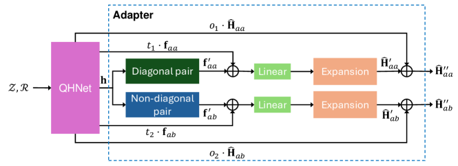
As outlined in Sec. 3.1, to facilitate the generalization of the Hamiltonian model in the OOD scenario, we apply self-consistency loss for fine-tuning the QHNet model with two fine-tuning approaches: all-param and adapter. Specifically, we construct the adapter using three modules: diagonal pair module, non-diagonal pair module and expansion module. and then insert it atop the original QHNet model. A schematic illustration of the adapter module is provided in Fig. C.1. Given the input molecule, the pretrained QHNet model is initially used to produce the initial Hamiltonian matrix blocks 555The model-predicted Hamiltonian should be formally denoted as , and we omit and for brevity, along with the final atomic representations and the final pairwise representations . Subsequently, the atomic representations are fed into corresponding diagonal or non-diagonal pair modules respectively to build pairwise representations . Afterward, the pairwise representations of the QHNet model and the adapter module are combined (e.g., , with as a learnable combination coefficient). The combined pairwise representations are first fed into a linear layer and then employed by the expansion module to produce the refinement Hamiltonian (). Finally, we take the combination of the initial Hamiltonian and the refinement Hamiltonian (e.g., , with as a learnable combination coefficient) as the final output . It is important to note that the combination of pairwise representations and Hamiltonian blocks, whether diagonal or non-diagonal, is conducted independently, and the combination coefficients are distinct for each pair (i.e., and ).
| Model | Ethanol | Malondialdehyde | Uracil |
|---|---|---|---|
| QHNet wo. self-con | 0.283 | 0.289 | 0.355 |
| QHNet w. self-con | 0.375 | 0.401 | 0.613 |
B.2 Self-Consistency Loss
Back-Propagation through Eigensolver.
As described in Sec. 2.3, the evaluation of self-consistency loss (Eq. (4)) requires the eigenvectors of the generalized eigenvalue problem (Line 3 in Alg. 1), necessitating the back-propagation through an eigensolver. Thus we need to compute the gradient of the loss function w.r.t the matrix . In our practical implementation, we solve the generalized eigenvalue problem for each molecule with two steps: (1) Solve the eigenvalue problem for matrix , and then define . This leads to the transformation of the Hamiltonian matrix to ; (2) Solve the eigenvalue problem for the transformed Hamiltonian matrix , , from which the eigenvectors of the original problem are recovered as . Following these steps, the self-consistency loss is calculated using the eigenvectors that have been derived.
The partial derivatives of self-consistency loss w.r.t the transformed matrix can be expressed as: , where
| (B.1) |
with representing the -th eigenvalues. The gradient is calculated using the chain rule , where and denote the vectorization operator and its inverse operator, denotes the Kronecker product operator, and denotes the -dimensional identity matrix. Then we can derive the partial derivative w.r.t the original Hamiltonian matrix as: . Consequently, the partial derivatives w.r.t rely on the matrix , which can lead to a large gradient when two eigenvalues are close.
To mitigate this instability and promote stable training, we introduce two treatments. The first is to limit the magnitude of gradient by applying truncation on matrix in the backward function of PyTorch:
| (B.2) |
where is a threshold determined by taking the 60-th percentile of absolute values of all entries. The technique is chosen for its simplicity and effectiveness, and there exist other methods for addressing this issue (Song et al., 2021; Wang et al., 2021a). The second treatment is to skip model parameter update when the scale of the gradient w.r.t parameters exceeds a certain threshold , which is determined through cross-validation.
Efficient Hamiltonian Reconstruction
To reconstruct the Hamiltonian , we first generate requisite integrals and quadrature grid using PySCF and then compute the Hamiltonian using PyTorch according to standard SCF procedure. Yet, this involves two costly steps. (1) Evaluating atomic basis functions on generated quadrature grid points is computationally expensive. To accelerate this computation, we re-implement the evaluation of basis functions on GPU. Moreover, the grid level determines the number of grid points and in turn influences the construction accuracy of the exchange-correlation potential . Empirically, we find that a grid level of 2 strikes an optimal balance between construction accuracy and computational efficiency. (2) The computation of the Hartree component entails a complexity (Line 6 in Alg. 1, is the number of electrons). As the molecular size increases, this computation becomes highly costly. To enable an efficient evaluation of the Hartree matrix, we apply the density fitting technique widely used in DFT programs to reduce the computational complexity from to . Leveraging the two techniques leads to a significant acceleration for the Hamiltonian reconstruction, enabling faster self-consistency training. Moreover, integral matrices that are solely dependent on the molecular conformation (i.e., , ) are pre-computed and stored in the database. These pre-computed matrices are then loaded as needed during the training process.
Computational Complexity.
As the self-consistency loss is constructed following the standard SCF procedure, it possesses the same computational complexity as one SCF iteration under the Kohn-Sham DFT formulation. After the application of the density fitting technique, the computational complexity becomes ( denotes the number of electrons in a molecule). Note that self-consistency training only brings extra computational cost during training, while keeps the same cost for Hamiltonian prediction. The empirical time cost of the Hamiltonian prediction model, both with and without the incorporation of self-consistency loss, are detailed in Table B.1.
Appendix C Experimental Study Settings
In this section, we provide further data preparation and training details for the empirical study presented in Sec. 3.
C.1 Dataset Preparation
To demonstrate the benefits of self-consistent training, we first conduct experiments on two generalization scenarios, corresponding to two molecular datasets, MD17 and QH9, respectively. Afterward, we evaluate the applicability of the Hamiltonian prediction model on large-scale molecules, for which we adopt the MD22 dataset.
| Molecule | Train (labeled) | Train (unlabeled) | Validation | Test | Molecular size |
|---|---|---|---|---|---|
| Ethanol | 100 | 24,900 | 500 | 4,500 | 9 |
| Malondialdehyde | 100 | 24,900 | 500 | 1,478 | 19 |
| Uracil | 100 | 24,900 | 500 | 4,500 | 26 |
MD17.
To evaluate the benefit of self-consistency training in improving generalization for the data-scare scenario, we adopt the MD17 dataset (Schütt et al., 2019), and focus on three conformational spaces of ethanol, malondialdehyde and uracil. The Hamiltonian matrices in this dataset are calculated with thePBE (Perdew et al., 1996) exchange-correlation functional and the Def2SVP Gaussian-type orbital (GTO) basis set. We follow the split setting used in Schütt et al. (2019) to divide the structures of each molecule into training/validation/test sets. Moreover, we randomly select 100 labels from the training set for supervised training, while the remaining training structures are utilized as unlabeled data for self-consistency training. The detailed statistics of three conformational spaces are summarized in Table C.1.
| Data setting | Training | Validation | Test |
|---|---|---|---|
| QH9-small | 94,001 | 10,000 | N/A |
| QH9-large | 18,000 | 2,000 | 6,830 |
| QH9-full | 124,289 | 6,542 | N/A |
QH9.
To evaluate the benefit of self-consistency training in improving generaliation for the out-of-distribution (OOD) scenario, we adopt the QH9 dataset666The dataset is licensed under a Creative Commons Attribution-NonCommercial-ShareAlike 4.0 International License. (Yu et al., 2023a). This dataset is proposed to benchmark Hamiltonian prediction methods in chemical space, consisting of two subsets: QH-stable and QH-dynamic. Here we adopt the QH-stable subset (dubbed as QH9 hereafter), which consists of 130,831 stable small organic molecules with no more than 9 heavy atoms, as well as their corresponding Hamiltonian matrices. The Hamiltonian matrices are calculated with the B3LYP (Becke, 1992) exchange-correlation functional and the Def2SVP GTO basis set. To simulate an OOD benchmark, we divide the QH9 dataset into two subsets by molecular size (QH9-small and QH9-large) and further partition them into training/validation/test sets. Additionally, we establish a separate split setting for the generalization study on large-scale molecules(referred to as QH9-full). Comprehensive statistics related to these division settings are detailed in Table C.2.
MD22.
To evaluate the applicability of the Hamiltonian prediction model on large-scale molecules, we adopt the MD22 dataset (Chmiela et al., 2023) and focus on the Ac-Ala3-NHMe (ALA3) and DHA molecules. Since the MD22 does not contain Hamiltonian labels, we randomly sample 500 structures for each molecule as our benchmark and use PySCF (Sun et al., 2018) to generate Hamiltonian matrices for these structures with the B3LYP exchange-correlation functional and the Def2SVP GTO basis set.
C.2 DFT Implementation Details
C.3 Hardware Configurations
All neural network models are trained and evaluated on a workstation equipped with a Nvidia A100 GPU with 80 GiB memory and a 24-core AMD EPYC CPU, which is also used for DFT calculations. Note that all the computation times reported in the empirical study are benchmarked on this specific hardware configuration to ensure consistency in comparison. However, it is also recognized that both neural network models and DFT computations have the potential to be parallelized and accelerated using multiple GPUs or CPU cores. Given this capability for parallel processing, establishing a perfectly equitable hardware benchmarking environment for both approaches is challenging.
C.4 Training Details
Data-Scarce Scenario.
We first describe the training details utilized in the empirical study of Sec. 3.1. For the self-consistency training setting, we set the total training iterations to 200k for three conformational spaces following (Yu et al., 2023b). Considering that the efficacy of the supervised learning setting might be limited by scarce labeled data, we allocate a higher number of training iterations (i.e., 500k) to this paradigm to ensure the model reaches its optimal performance within the constraints of the available labels. For all experimental conditions and datasets, we maintain a consistent batch size of 5. We utilize a polynomial decay learning rate scheduler to modulate the learning rate (LR) during training, where the polynomial power is set to 5 for self-consistency training and 14 for supervised learning based on empirical trials. Notably, the scheduler increases the learning rate gradually during the first 10k warm-up iterations. The learning rate starts at 0 and peaks at a maximum of 1 across all training scenarios. When addressing the supervised training settings with extended labeled data as mentioned in Sec. 3.2, we adopt the same training hyperparameters as those used in the supervised learning setting of Sec. 3.1, with the singular adjustment of setting the polynomial power to 5.
Out-of-Distribution Scenario.
As outlined in Sec. 3.1, to benchmark the OOD generalization performance, we initially train the QHNet model on the QH9-small subset, and then fine-tune the model on unlabeled large molecules. We continue to use the polynomial learning rate schedule, which includes a warm-up phase. Additional training hyperparameters are detailed in Table C.3.
| Training Phase | Batch size | Maximum LR | Polynomial Power | Iterations | Warm-up Iterations |
|---|---|---|---|---|---|
| Pretraining | 32 | 5 | 1 | 300k | 1k |
| Fine-tuning | 5 | 2 | 8 | 200k | 3k |
Large-Scale Molecular Systems.
As discussed in Sec. 3.3, we adopt a two-stage training strategy to generalize the Hamiltonian model to large-scale MD22 structures. We still employ the polynomial learning rate schedule with the warm-up stage, and detail other training hyper-parameters in Table C.4.
| Training Phase | Batch size | Maximum LR | Polynomial Power | Iterations | Warm-up Iterations |
|---|---|---|---|---|---|
| Pretraining | 32 | 5 | 1 | 400k | 5k |
| Fine-tuning (ALA3) | 2 | 2 | 8 | 100k | 10k |
| Fine-tuning (DHA) | 1 | 2 | 8 | 200k | 10k |
| Molecule | Setting | SCF Accel. | ||||||
|---|---|---|---|---|---|---|---|---|
| Ethanol | extended-label | 58.28 | 986.84 | 99.94 | 230.20 | 2902.14 | 2723.64 | 63.5 |
| label + self-con | 95.90 | 340.56 | 99.94 | 403.60 | 1426.20 | 1370.35 | 61.5 | |
| Malondi- | extended-label | 71.45 | 1014.12 | 99.63 | 199.48 | 414.58 | 415.91 | 66.6 |
| aldehyde | label + self-con | 86.60 | 280.39 | 99.67 | 274.45 | 279.14 | 324.37 | 62.1 |
| Uracil | extended-label | 52.53 | 288.29 | 99.38 | 306.05 | 294.54 | 398.08 | 58.1 |
| label + self-con | 63.82 | 315.40 | 99.58 | 359.98 | 369.67 | 388.30 | 54.5 |
| Model | |||||||||
|---|---|---|---|---|---|---|---|---|---|
| QH9 (valid) | ALA3 | DHA | QH9 (valid) | ALA3 | DHA | QH9 (valid) | ALA3 | DHA | |
| e2e (ET) | 818.77 | 1.74 | 2.92 | 540.22 | 7.72 | 2.58 | 1.38 | 2.38 | 3.39 |
| e2e (Equiformer) | 646.42 | 2.38 | 3.76 | 488.40 | 1.16 | 2.31 | 1.15 | 2.27 | 4.17 |
Appendix D Additional Experimental Results
D.1 Generalization Results
As noted in Sec. 3.1, while supervised training can outperform self-consistency training with adequate computational resources, the advantage in terms of Hamiltonian MAE does not consistently extend to molecular properties. This discrepancy has been observed in the OOD generalization scenario in Table 3 of Sec. 3.1. Correspondingly, the results presented in Table C.5 show that there exists a comparable trend in the data-scarce scenario.
D.2 Amortization Effect of Self-Consistency Training
As mentioned in Sec. 3.2, we directly access the amortization effect by comparing the computational cost of self-consistency training with that of DFT for solving a bunch of structures. It should be noted that measuring the computational cost of DFT on all unlabeled training structures is impractical, thus we run DFT on 50 randomly picked structures for each molecule. The mean computation time derived from these 50 structures serves as a benchmark to approximate the overall computational time required for the complete set of structures.
D.3 Large-Scale Generalization Results
As discussed in Sec. 3.3, we assess the generalization of self-consistency training to large-scale MD22 structures by comparing it with two state-of-the-art end-to-end (e2e) property prediction models. For this purpose, we choose two advanced e2e architectures, ET777https://github.com/torchmd/torchmd-net, the code is freely available under the terms of the MIT license. (Thölke & De Fabritiis, 2021) and Equiformer888https://github.com/atomicarchitects/equiformer, the code is freely available under the terms of the MIT license. (Liao & Smidt, 2022), as our baselines. They are representatives for equivariant architectures that utilize vector features and high-order tensor features, respectively. Despite the availability of pretrained models for these methods, they are not directly applicable for our analysis because they were originally trained on the QM9 dataset, which differs from the QH9 dataset used in our study. The two datasets use distinct orbital basis sets for DFT calculations, resulting in slightly different label distributions. To ensure a fair comparison, we retrain the ET and Equiformer models on the QH9 dataset, with the default hyper-parameter settings specified in their codebases. The performance of the two e2e models on the QH9 validation set, as shown in Table C.6, aligns with the outcomes reported in their respective original publications, validating the effectiveness of our model replication. The substantial performance disparity between the QH9 validation set and two MD22 molecules implies a significant generalization challenge for e2e models. Fortunately, this challenge can be potentially alleviated by applying self-consistency training to Hamiltonian prediction.
Appendix E Limitations and Future work
Even though self-consistency training has shown improved efficiency than conventional DFT calculation for training a Hamiltonian prediction model or for solving a bunch of molecular structures (Sec. 3.2) by amortizing the cost of SCF iterations over queried molecular structures, the computational complexity remains the same as that of DFT. This complexity may still limit the applicability (but to a higher level) of Hamiltonian prediction to large molecular systems such as biomacromolecules. It would be a promising future work to reduce the complexity of evaluating the self-consistency loss by leveraging techniques from linear-scaling DFT algorithms. The Hamiltonian prediction model we used in this study, although is already more efficient than a few alternatives, still requires considerable cost to evaluate, due to e.g. the use of computationally expensive tensor product operations. This calls for designing more efficient neural network architectures for Hamiltonian prediction. Moreover, current Hamiltonian prediction models only support prediction under a specific basis set, which has a restricted flexibility to trade-off efficiency and accuracy, and is hard to leverage data under different choices of basis. A possible solution to this restriction is including the overlap matrix into the model input, which conveys information about the basis set in a form relevant to the given molecular structure.