Memoryless concretization relation

Abstract

We introduce the concept of memoryless concretization relation ($\operatorname{MCR}$) to describe abstraction within the context of controller synthesis. This relation is a specific instance of alternating simulation relation ($\operatorname{ASR}$), where it is possible to simplify the controller architecture. In the case of $\operatorname{ASR}$, the concretized controller needs to simulate the concurrent evolution of two systems, the original and abstract systems, while for $\operatorname{MCR}$, the designed controllers only need knowledge of the current concrete state. We demonstrate that the distinction between $\operatorname{ASR}$ and $\operatorname{MCR}$ becomes significant only when a non-deterministic quantizer is involved, such as in cases where the state space discretization consists of overlapping cells. We also show that any abstraction of a system that alternatingly simulates a system can be completed to satisfy $\operatorname{MCR}$ at the expense of increasing the non-determinism in the abstraction. We clarify the difference between the $\operatorname{MCR}$ and the feedback refinement relation ($\operatorname{FRR}$), showing in particular that the former allows for non-constant controllers within cells. This provides greater flexibility in constructing a practical abstraction, for instance, by reducing non-determinism in the abstraction. Finally, we prove that this relation is not only sufficient, but also necessary, for ensuring the above properties.

I Introduction

Abstraction-based control techniques involve synthesizing a correct-by-construction controller through a systematic three-step procedure illustrated on Figure 1. First, both the original system and the specifications are transposed into an abstract domain, resulting in an abstract system and corresponding abstract specifications. In this paper, we refer to the original system as the concrete system as opposed to the abstract system. Next, an abstract controller is synthesized to solve this abstract control problem. Finally, in the third step, called concretization as opposed to abstraction, a controller for the original control problem is derived from the abstract controller. The value of this approach lies in the substitution of the concrete system (often a system with an infinite number of states) with a finite state system, which makes it possible to leverage powerful control tools (see [2, 3]), for example from graph theory, such as Dijkstra, the $A^{*}$ algorithm or dynamic programming, allowing to design correct-by-construction controllers, often with rigorous (safety, or performance) guarantees. Abstraction-based controller design crucially relies on the existence of a simulation relation between the concrete and abstract states, allowing to infer the control actions in the concrete system from the ones actuated in the corresponding states of the abstract system. Most approaches are based on the alternating simulation relation ($\operatorname{ASR}$) [4], which provides a framework for guaranteeing a concretization step that provably ensures the specifications for the concrete system.

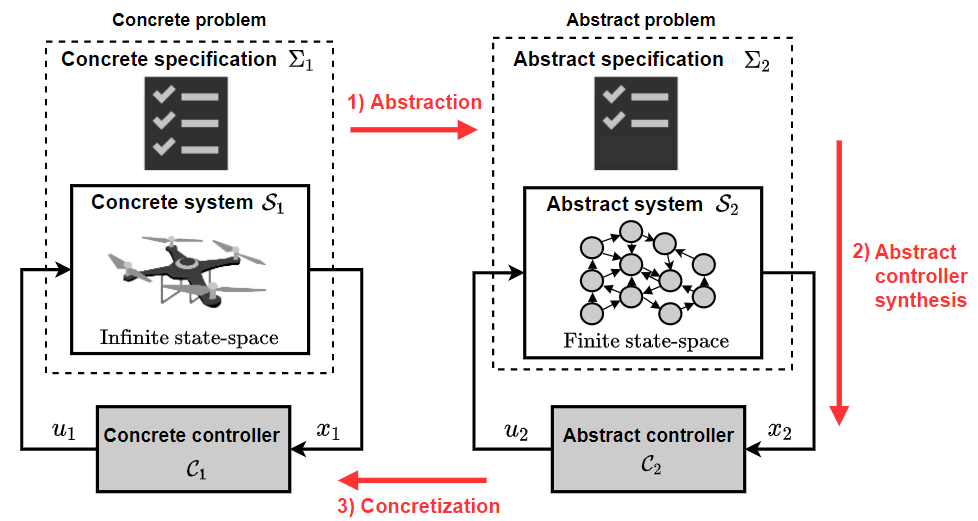
Figure 1: The three steps of abstraction-based control. Our work focuses on the algorithmic burden necessary for the third step, and characterizes the relation between the systems allowing for a memoryless algorithm at step three.

Although the alternating simulation relation offers a safety critical framework, it has several practical drawbacks. The first issue is that this relation provides no complexity guarantee on the concretization procedure, i.e., the concrete controller could contain the entire abstraction (which is typically made up of millions of states and transitions) as a building block, we refer to this problem as the concretization complexity issue. See [5, Proposition 8.7] for a description of the algorithmic concretization procedure. The second limitation is that, although $\operatorname{ASR}$ guarantees the existence of a controller for the concrete system such that the closed-loop systems share the same behavior, it does not guarantee that some of these properties will be transferred to the concrete controller during the concretization step.

For this reason, various relations have been introduced in the literature, e.g. [6, 7, 8, 9], to tackle specific shortcomings of the alternating simulation relation. Some works propose abstraction-based techniques that do not suffer from this concretization complexity issue, but they are either limited to subsets of specification such as safety or reachability [10, 11, 12, 13], or for a specific class of dynamical systems, e.g. incrementally stable  [10], piecewise affine (PWA) dynamics [14]. Other abstraction-based controller synthesis methods circumvent the concretization complexity issue by constructing abstractions without overlapping cells [15, 14, 12, 16, 17, 18]. In particular, in [6], the authors present the feedback refinement relation ($\operatorname{FRR}$) which provides a framework for an extremely simple controller architecture, which is not restricted to certain types of specifications or systems, and, as we shall see, forms the basis of our reflection.

In this paper, we study the properties that a simulation relation might require, and establish their implications on controller design characteristics. Specifically, we analyze how the relation established between the concrete and abstract systems during the abstraction phase affects the concretization process, while the methods used to compute abstractions or solve the resulting abstract control problems are beyond the scope of this work. We introduce the memoryless concretization relation ($\operatorname{MCR}$) which guarantees a simple control architecture for the concrete system that is not problem-specific. Unlike the general case of alternating simulation relation, the controller only needs information about the current concrete state and does not need to simulate the concurrent evolution of the concrete and abstract systems. We show that in the specific case of a deterministic quantizer (that is, a single-valued map), alternating simulation relation and memoryless concretization relation coincide. As a consequence, the memoryless concretization relation turns out to be essential in the context of an abstraction composed of overlapping cells, a framework we consider crucial for building a non-trivial smart abstraction, see [8]. We prove that $\operatorname{MCR}$ is not only sufficient to guarantee the functionality of this memoryless controller architecture, but also necessary for it to work with all abstract controllers, i.e., regardless of the specifications. Finally, we propose an in-depth discussion of feedback refinement relation which turns out to be a special case of memoryless concretization relation, with the additional requirement to use only symbolic state information. As a result, feedback refinement relation is limited to the design of piecewise constant controllers, whereas memoryless concretization relation allows the design of piecewise state-dependent controllers. We illustrate on a simple example the advantage of memoryless concretization relation over feedback refinement relation when concrete state information is available.

Notation: The sets $\mathbb{R},\mathbb{Z},\mathbb{Z}_{+}$ denote respectively the sets of real numbers, integers and non-negative integer numbers. For example, we use $[a,b]\subseteq\mathbb{R}$ to denote a closed continuous interval and $[a;b]=[a,b]\cap\mathbb{Z}$ for discrete intervals. The symbol $\varnothing$ denotes the empty set. Given two sets $A,B$, we define a single-valued map as $f:A\rightarrow B$, while a set-valued map is defined as $f:A\rightarrow 2^{B}$, where $2^{B}$ is the power set of $B$, i.e., the set of all subsets of $B$. The image of a subset $\Omega\subseteq A$ under $f:A\rightarrow 2^{B}$ is denoted $f(\Omega)$. We identify a binary relation $R\subseteq A\times B$ with set-valued maps, i.e., $R(a)=\{b\mid(a,b)\in R\}$ and $R^{-1}(b)=\{a\mid(a,b)\in R\}$. Given a set $A$, we denote the binary identity relation $Id_{A}\subseteq A\times A$ such that $(x,y)\in Id_{A}\Leftrightarrow x=y$. A relation $R\subseteq A\times B$ is strict and single-valued if for every $a\in A$ the set $R(a)\neq\varnothing$ and $R(a)$ is a singleton, respectively. Given two set-valued maps $f,g$, we denote by $f\circ g$ their composition $(f\circ g)(x)=f(g(x))$. If $R\subseteq A\times B$ and $Q\subseteq B\times C$, then their composition $R\circ Q=\{(a,c)\in A\times C\ \mid\exists b\in B\text{ such that }(a,b)\in R\text{ and }(b,c)\in Q\}$.

II Preliminaries

In this section, we start by defining the considered control framework, i.e., the systems, the controllers and the specifications.

We consider dynamical systems of the following form.

Definition 1.

A transition control system is a tuple $\mathcal{S}\coloneqq(\mathcal{X},\mathcal{U},F)$ where $\mathcal{X}$ and $\mathcal{U}$ are respectively the set of states and inputs and the set-valued map $F:\mathcal{X}\times\mathcal{U}\rightarrow 2^{\mathcal{X}}$ where $F(x,u)$ give the set of states that can be reached from a given state $x$ under a given input $u$. $\bigtriangledown$

We introduce the set-valued operator of available inputs, defined as $\mathcal{U}_{F}(x)=\{u\in\mathcal{U}\mid F(x,u)\neq\varnothing\}$, which give the set of inputs $u$ available at a given state $x$. When it is clear from the context which system it refers to, we simply write the available inputs operator $\mathcal{U}(x)$. In this paper, we consider non-blocking systems, i.e., $\forall x\in\mathcal{X}:\mathcal{U}(x)\neq\varnothing$.

The use of a set-valued map to describe the transition map of a system allows to model perturbations and any kind of non-determinism in a common formalism. We say that a transition control system is deterministic if for every state $x\in\mathcal{X}$ and control input $u\in\mathcal{U}$, $F(x,u)$ is either empty or a singleton. Otherwise, we say that it is non-deterministic. A finite-state system, in contrast to an infinite-state system, refers to a system characterized by finitely many states and inputs.

A tuple $(\bm{x},\bm{u})\in\mathcal{X}^{[0;T[}\times\mathcal{U}^{[0;T-1[}$ is a trajectory of length $T$ of the system $\mathcal{S}=(\mathcal{X},\mathcal{U},F)$ starting at $x(0)$ if $T\in\mathbb{N}\cup\{\infty\}$, $x(0)\in\mathcal{X}$, $\forall k\in[0;T-1[:u(k)\in\mathcal{U}(x(k))$ and $x(k+1)\in F(x(k),u(k))$. The set of trajectories of $\mathcal{S}$ is called the behavior of $\mathcal{S}$, denoted $\mathcal{B}(\mathcal{S})$.

Definition 2.

Let $\mathcal{S}=(\mathcal{X},\mathcal{U},F)$. The set $\mathcal{B}(\mathcal{S})=\{(\bm{x},\bm{u})\mid\exists T\in\mathbb{N}\cup\{\infty\}\text{ such that }(\bm{x},\bm{u})\text{ is a trajectory of }\mathcal{S}\text{ of length }T\},$ is called the behavior of $\mathcal{S}$. We define the state behavior $\mathcal{B}_{x}(\mathcal{S})$ as $\bm{x}\in\mathcal{B}_{x}(\mathcal{S})\Leftrightarrow\exists\bm{u}:(\bm{x},\bm{u})\in\mathcal{B}(\mathcal{S})$.

It is a common practice in the abstraction-based framework to represent systems with an extra set $\mathcal{Y}$ for outputs, and an output mapping function $H:\mathcal{X}\rightarrow\mathcal{Y}$. In that case, the states in $\mathcal{X}$ are seen as internal to the system, while the outputs are externally visible. However, as this is not essential to our current discussion, we exclude it here.

We consider systems without internal variables, see [1, Definition III.1] and the discussion that follows this definition. This extension is necessary to correctly define the composition of a system with a dynamic controller. For the sake of clarity and to avoid the use of internal variables, we only consider static controllers.

Definition 3.

We define a static controller for a system $\mathcal{S}=(\mathcal{X},\mathcal{U},F)$ as a set-valued map $\mathcal{C}:\mathcal{X}\rightarrow 2^{\mathcal{U}}$ such that $\forall x\in\mathcal{X}:\ \mathcal{C}(x)\subseteq\mathcal{U}(x)$, $\mathcal{C}(x)\neq\varnothing$. We define the controlled system, denoted as $\mathcal{C}\times\mathcal{S}$, as the transition system characterized by the tuple $(\mathcal{X},\mathcal{U},F_{\mathcal{C}})$ where $x^{\prime}\in F_{\mathcal{C}}(x,u)\Leftrightarrow(u\in\mathcal{C}(x)\land x^{\prime}\in F(x,u))$.

This controller is static since the set of control inputs enabled at a given state only depend on the state. A more general notion of controller (called a dynamic controller) would take the entire past trajectory and/or other variables as input. For the sake of clarity we limit ourselves to static controllers although most definitions and proofs extend easily to dynamical controllers.

We now define the control problem.

Definition 4.

Consider a system $\mathcal{S}=(\mathcal{X},\mathcal{U},F)$. A specification $\Sigma$ for $\mathcal{S}$ is defined as any subset $\Sigma\subseteq(\mathcal{X}\times\mathcal{U})^{\infty}$. It is said that system $\mathcal{S}$ satisfies the specification $\Sigma$ if $\mathcal{B}(\mathcal{S})\subseteq\Sigma$. A system $\mathcal{S}$ together with a specification $\Sigma$ constitute a control problem $(\mathcal{S},\Sigma)$. Additionally, a controller $\mathcal{C}$ is said to solve the control problem $(\mathcal{S},\Sigma)$ if $\mathcal{C}\times\mathcal{S}$ satisfies the specification $\Sigma$.

Given $\mathcal{X}_{I},\mathcal{X}_{T},\mathcal{X}_{O}\subseteq\mathcal{X}$, we define the specific reach-avoid specification that we will use to motivate new relations

$$\Sigma^{\text{Reach}}=\{ (\bm{x},\bm{u})\in(\mathcal{X}\times\mathcal{U})^{\infty}\mid x(0)\in\mathcal{X}_{I}\Rightarrow$$

$$\exists k\in\mathbb{Z}_{+}:\left(x(k)\in\mathcal{X}_{T}\land\forall k^{\prime}\in[0;k):x(k^{\prime})\notin\mathcal{X}_{O}\right)\},$$ (1)

which enforces that all states in the initial set $\mathcal{X}_{I}$ will reach the target $\mathcal{X}_{T}$ in finite time while avoiding obstacles in $\mathcal{X}_{O}$. We use the abbreviated notation $\Sigma^{\text{Reach}}=[\mathcal{X}_{I},\mathcal{X}_{T},\mathcal{X}_{O}]$ to denote the specification (1).

III Alternating simulation relation

In this paper, we will refer to $\mathcal{S}_{1}=(\mathcal{X}_{1},\mathcal{U}_{1},F_{1})$ as the concrete system and $\mathcal{S}_{2}=(\mathcal{X}_{2},\mathcal{U}_{2},F_{2})$ as its abstraction.

In practice, the abstract domain $\mathcal{X}_{2}$ of $\mathcal{S}_{2}$ is constructed by discretizing the concrete state space $\mathcal{X}_{1}$ of $\mathcal{S}_{1}$ into subsets (called cells). The discretization is induced by the relation $R\subseteq\mathcal{X}_{1}\times\mathcal{X}_{2}$, i.e., the cell associated with the abstract state $x_{2}\in\mathcal{X}_{2}$ is $R^{-1}(x_{2})\subseteq\mathcal{X}_{1}$. Note that in this context, we refer to the set-valued map $R(x_{1})=\{x_{2}\mid(x_{1},x_{2})\in R\}$ as the quantizer. When $R$ is a single-valued map, we refer to it as defining a partition of $\mathcal{X}_{1}$, in contrast to the case of set-valued maps where we say that it defines a cover of $\mathcal{X}_{1}$, see Figure 2 for clarity. Notably, the condition that $R$ is a strict relation is equivalent to ensuring that the discretization completely covers $\mathcal{X}_{1}$.

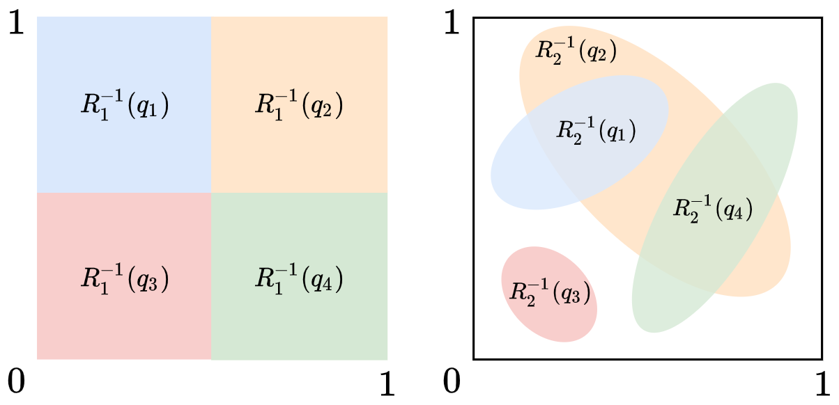
Figure 2: Types of discretization of the concrete state space. Let $\mathcal{S}_{1}=(\mathcal{X}_{1},\mathcal{U}_{1},F_{1})$ with $\mathcal{X}_{1}=[0,1]^{2}$, $\mathcal{S}_{2}=(\mathcal{X}_{2},\mathcal{U}_{2},F_{2})$ with $\mathcal{X}_{2}=\{q_{1},q_{2},q_{3},q_{4}\}$, $R_{1}\subseteq\mathcal{X}_{1}\times\mathcal{X}_{2}$ and $R_{2}\subseteq\mathcal{X}_{1}\times\mathcal{X}_{2}$ are explicit from the figure. Left: $R_{1}$ is a strict single-valued map, i.e., it induces a full partition of $\mathcal{X}_{1}$. Right: $R_{2}$ is a non-strict set-valued map, i.e., it induces a partial cover of $\mathcal{X}_{1}$.

As mentioned in the introduction, the concrete specification $\Sigma_{1}$ must also be translated into an abstract specification $\Sigma_{2}$. For example, given $\Sigma_{1}^{\text{Reach}}=[\mathcal{X}_{I},\mathcal{X}_{T},\mathcal{X}_{O}]$ with $\mathcal{X}_{I},\mathcal{X}_{T},\mathcal{X}_{O}\subseteq\mathcal{X}_{1}$, the abstract specification $\Sigma_{2}^{\text{Reach}}=[\mathcal{Q}_{I},\mathcal{Q}_{T},\mathcal{Q}_{O}]$ with $\mathcal{Q}_{I},\mathcal{Q}_{T},\mathcal{Q}_{O}\subseteq\mathcal{X}_{2}$ must satisfy the following conditions $R(\mathcal{X}_{I})\subseteq\mathcal{Q}_{I}$, $\mathcal{Q}_{T}\subseteq R(\mathcal{X}_{T})$ and $R(\mathcal{X}_{O})\subseteq\mathcal{Q}_{O}$.

Given an abstract controller $\mathcal{C}_{2}$ that solves the control problem $(\mathcal{S}_{2},\Sigma_{2})$, to guarantee the existence of a controller $\mathcal{C}_{1}$ that solves the concrete problem $(\mathcal{S}_{1},\Sigma_{1})$, the tuple $(\mathcal{S}_{1},\mathcal{S}_{2},R)$ must satisfy the following controlled simulability property, which guarantees that the behavior of the concrete controlled system $\mathcal{C}_{1}\times\mathcal{S}_{1}$ is simulated by the abstract controlled system $\mathcal{C}_{2}\times\mathcal{S}_{2}$ via the relation $R$.

Property 1 (Controlled simulability property-[1, (5)]).

Given two systems $\mathcal{S}_{1}$ and $\mathcal{S}_{2}$, and a relation $R\subseteq\mathcal{X}_{1}\times\mathcal{X}_{2}$, we say that the tuple $(\mathcal{S}_{1},\mathcal{S}_{2},R)$ satisfies the controlled simulability property if for every controller $\mathcal{C}_{2}$ there exists a (possibly non-static) controller $\mathcal{C}_{1}$ such that for every trajectory $\bm{x}_{1}$ of length $T$ of the controlled system $\mathcal{C}_{1}\times\mathcal{S}_{1}$, there exists a trajectory $\bm{x}_{2}$ of length $T$ of the controlled system $\mathcal{C}_{2}\times\mathcal{S}_{2}$ satisfying

$$\forall k\in[0;T-1]:\ (x_{1}(k),x_{2}(k))\in R.$$ (2)

The condition (2) can be equivalently reformulated as follows

$$\mathcal{B}_{x}(\mathcal{C}_{1}\times\mathcal{S}_{1})\subseteq R^{-1}(\mathcal{B}_{x}(\mathcal{C}_{2}\times\mathcal{S}_{2})).$$ (3)

Controlled simulability can be used to guarantee that properties satisfied by the abstract controlled system $\mathcal{C}_{2}\times\mathcal{S}_{2}$ are also satisfied by the concrete controlled system $\mathcal{C}_{1}\times\mathcal{S}_{1}$. To design $\mathcal{C}_{1}$ from $\mathcal{C}_{2}$ in 1, the relation must impose conditions on the local dynamics of the systems in the associated states, accounting for the impact of different input choices on state transitions. The alternating simulation relation [5, Definition 4.19] is a comprehensive definition of such a relation. It guarantees that any control applied to $\mathcal{S}_{2}$ can be concretized into a controller for $\mathcal{S}_{1}$ that maintains the relation between the controlled trajectories.

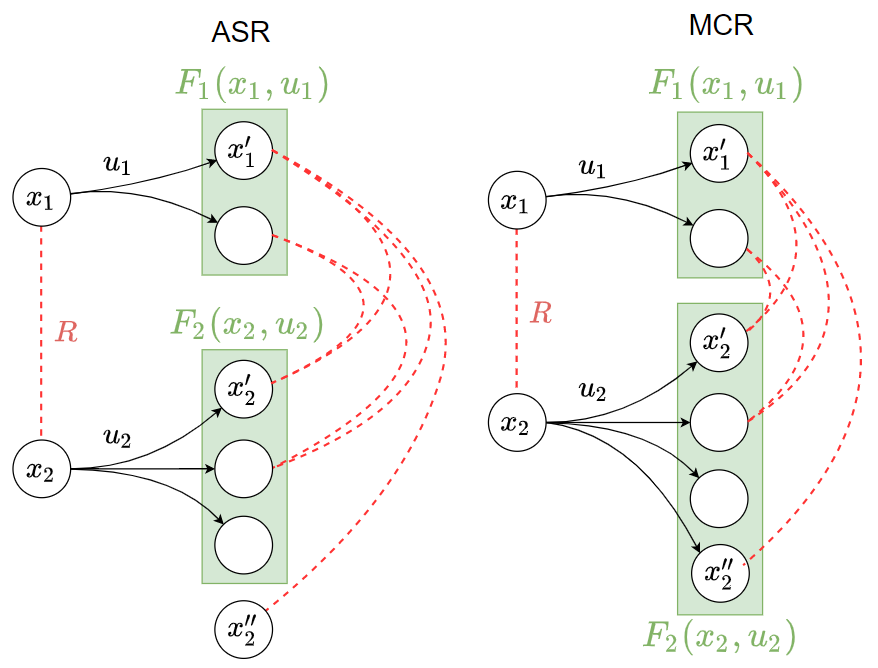
Figure 3: Local conditions between related states to satisfy the relation. Note that here, the relation is fixed (i.e., here a cover of the state space since $|R(x_{1}^{\prime})|>1$) as well as the transition map of the concrete system and that we are simply changing the transition map of the abstract system. Left: The relation $R$ is a $\operatorname{ASR}$ but not a $\operatorname{MCR}$. Right: The relation $R$ is a $\operatorname{MCR}$.

Definition 5 ($\operatorname{ASR}$).

A relation $R\subseteq\mathcal{X}_{1}\times\mathcal{X}_{2}$ is an alternating simulation relation from $\mathcal{S}_{1}$ to $\mathcal{S}_{2}$ if for every $(x_{1},x_{2})\in R$ and for every $u_{2}\in\mathcal{U}_{2}(x_{2})$ there exists $u_{1}\in\mathcal{U}_{1}(x_{1})$ such that for every $x_{1}^{\prime}\in F_{1}(x_{1},u_{1})$ there exists $x_{2}^{\prime}\in F_{2}(x_{2},u_{2})$ such that $(x_{1}^{\prime},x_{2}^{\prime})\in R$.

Note that sometimes one prefers to speak of the extended relation $R_{e}\subseteq\mathcal{X}_{1}\times\mathcal{X}_{2}\times\mathcal{U}_{1}\times\mathcal{U}_{2}$, which is defined by the set of $(x_{1},x_{2},u_{1},u_{2})$ satisfying the condition given in the definition of $R$. When it refers to a $\operatorname{ASR}$, we denote it $R_{e}^{\operatorname{ASR}}$.

The local condition stated in Definition 5 is illustrated for some $(x_{1},x_{2},u_{1},u_{2})\in R_{e}^{\operatorname{ASR}}$ in Figure 3 (left). The fact that $R$ is an alternating simulation relation from $\mathcal{S}_{1}$ to $\mathcal{S}_{2}$ will be denoted $\mathcal{S}_{1}\preceq_{R}^{\operatorname{ASR}}\mathcal{S}_{2}$, and we write $\mathcal{S}_{1}\preceq^{\operatorname{ASR}}\mathcal{S}_{2}$ if $\mathcal{S}_{1}\preceq_{R}^{\operatorname{ASR}}\mathcal{S}_{2}$ holds for some $R$.

Note that this definition slightly differs from [5, Definition 4.19], where there is an additional requirement regarding the outputs of related states. This requirement is useful for the concept of approximate alternating simulation relation [5, Definition 9.6] which we do not discuss here.

One needs an interface to map abstract inputs to concrete ones.

Definition 6 (Interface).

Given two systems $\mathcal{S}_{1}$ and $\mathcal{S}_{2}$, a relation $R$ of type $\operatorname{T}$, i.e. $\mathcal{S}_{1}\preceq_{R}^{\operatorname{T}}\mathcal{S}_{2}$, and its associated extended relation $R_{e}^{\operatorname{T}}$, a map $I_{R}^{\operatorname{T}}:\mathcal{X}_{1}\times\mathcal{X}_{2}\times\mathcal{U}_{2}\rightarrow 2^{\mathcal{U}_{1}}$ is an interface from $\mathcal{S}_{2}$ to $\mathcal{S}_{1}$ if:
$\forall(x_{1},x_{2})\in R,\ \forall u_{2}\in\mathcal{U}_{2}(x_{2})$,

$$I_{R}^{\operatorname{T}}(x_{1},x_{2},u_{2}) \neq\varnothing$$ (4)

$$I_{R}^{\operatorname{T}}(x_{1},x_{2},u_{2}) \subseteq\{u_{1}\mid(x_{1},x_{2},u_{1},u_{2})\in R_{e}^{\operatorname{T}}\}.$$ (5)

The maximal interface associated to $R$ satisfies $I_{R}^{\operatorname{T}}(x_{1},x_{2},u_{2})=\{u_{1}\mid(x_{1},x_{2},u_{1},u_{2})\in R_{e}^{\operatorname{T}}\}$.

Theorem 1.

Let two systems $\mathcal{S}_{1}$ and $\mathcal{S}_{2}$, and a relation $R$ such that $\mathcal{S}_{1}\preceq_{R}^{\operatorname{ASR}}\mathcal{S}_{2}$, an interface $I_{R}^{\operatorname{ASR}}$, and any trajectories $(\bm{x}_{1},\bm{u}_{1})$ and $(\bm{x}_{2},\bm{u}_{2})$ of length $T$ where $T\in\mathbb{N}\cup\{\infty\}$ such that $(x_{1}(0),x_{2}(0))\in R$ and

$$u_{2}(k) \in\mathcal{U}_{2}(x_{2}(k)) k\in[0;T-1[;$$

$$u_{1}(k) \in I_{R}^{\operatorname{ASR}}(x_{1}(k),x_{2}(k),u_{2}(k)) k\in[0;T-1[;$$

$$x_{1}(k+1) \in F_{1}(x_{1}(k),u_{1}(k)) k\in[0;T-1[;$$

$$x_{2}(k+1) \in F_{2}(x_{2}(k),u_{2}(k))\cap R(x_{1}(k+1)) k\in[0;T-1[.$$

Then, the following holds

$$(\bm{x}_{1},\bm{u}_{1}) \in\mathcal{B}(\mathcal{S}_{1}),$$

$$(\bm{x}_{2},\bm{u}_{2}) \in\mathcal{B}(\mathcal{S}_{2}),$$

$$\forall k\in[0;T-1]: \ (x_{1}(k),x_{2}(k))\in R.$$

Proof.

We proceed by induction on $k$. Given that $(x_{1}(k),x_{2}(k))\in R$, which is true for $k=0$. Since $\mathcal{S}_{1}\preceq_{R}^{\operatorname{ASR}}\mathcal{S}_{2}$, and according to (4) and (5), for every $u_{2}(k)\in\mathcal{U}_{2}(k)$, there exists $u_{1}(k)\in I_{R}^{\operatorname{ASR}}(x_{1}(k),x_{2}(k),u_{2}(k))\subseteq\mathcal{U}_{1}(x_{1}(k))$. Furthermore, since $\mathcal{S}_{1}\preceq_{R}^{\operatorname{ASR}}\mathcal{S}_{2}$, we can conclude that $F_{2}(x_{2}(k),u_{2}(k))\cap R(x_{1}(k+1))\neq\varnothing$, ensuring that $(x_{1}(k+1),x_{2}(k+1))\in R$. ∎

Theorem 2.

Given two systems $\mathcal{S}_{1}$ and $\mathcal{S}_{2}$, if $\mathcal{S}_{1}\preceq_{R}^{\operatorname{ASR}}\mathcal{S}_{2}$, then $(\mathcal{S}_{1},\mathcal{S}_{2},R)$ satisfies the controlled simulability property (1).

Proof.

Given a controller $\mathcal{C}_{2}$, we can define a controller $\mathcal{C}_{1}$ implementing the algorithm given in Theorem 1 by taking $u_{2}(k)\in\mathcal{C}_{2}(x_{2}(k))\subseteq\mathcal{U}_{2}(x_{2}(k))$, which ensure that $(\mathcal{S}_{1},\mathcal{S}_{2},R)$ satisfies the controlled simulability property. ∎

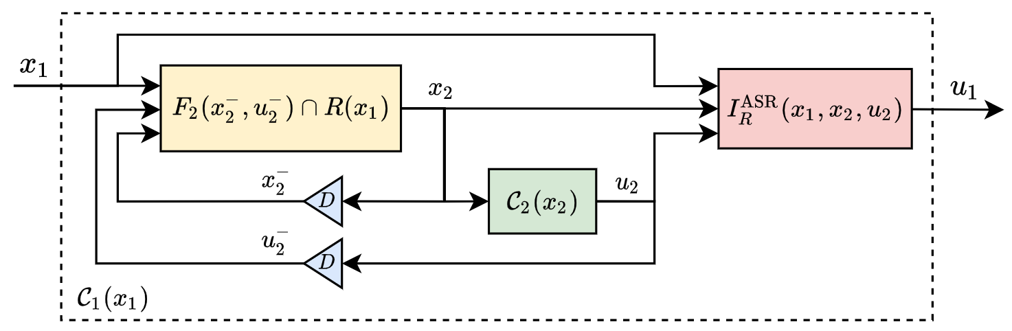
Figure 4: Dynamic controller architecture $\mathcal{C}_{1}$ such that $(\mathcal{S}_{1},\mathcal{S}_{2},\mathcal{C}_{1},\mathcal{C}_{2},R)$ satisfies the controlled simulability property if $\mathcal{S}_{1}\preceq_{R}^{\operatorname{ASR}}\mathcal{S}_{2}$. The red block is the interface $I_{R}^{\operatorname{ASR}}$. The yellow block contains the abstract system and the quantizer. The green block is the abstract controller. The blue blocks are delay blocks which represent memory elements that store and provide a past value of a signal, e.g., $D(x_{2}(k))=x_{2}(k-1)$.

From Theorem 1, we can construct a concrete controller $\mathcal{C}_{1}$, whose block diagram is given in Figure 4, guaranteeing the controlled simulability property. This concrete controller simulates the abstraction at every time step which can be computationally expensive if $F_{2}$ is hard to compute, e.g., if $F_{1}$ itself is hard to compute (or approximate). This is what we refer to as the concretization complexity issue. In addition, the proposed controller architecture $\mathcal{C}_{1}$ requires memory to account for last past abstract input and state, as illustrated on the block diagram in Figure 4.

Note that $\mathcal{S}_{1}\preceq^{\operatorname{ASR}}\mathcal{S}_{2}$ guarantees that $(\mathcal{S}_{1},\mathcal{S}_{2},R)$ satisfies controlled simulability property. Nevertheless, this does not guarantee that any arbitrary property of $\mathcal{C}_{2}$ will be translated in $\mathcal{C}_{1}$. In particular the property of a controller being static is certainly not preserved. This will be illustrated in the next section. Another downside is that the controller given here requires simulating the abstract system at every step to know which inputs to allow in the concrete case.

Theorem 1 does not appear formally in [5], but it is suggested in the discussion that follows  [5, Def 6.1-Feedback composition]. The content of Theorem 2 was mostly implied in the discussion around [5, Prop 8.7]. In this light, Section III gives the necessary background, in standardized form, for the introduction of the memoryless concretization relation.

IV Memoryless concretization relation

We start by defining the concrete controller resulting from a specific concretization scheme.

Definition 7 (Memoryless concretized controller).

Given two systems $\mathcal{S}_{1}$ and $\mathcal{S}_{2}$, a strict relation $R$ of type $\operatorname{T}$, an interface $I_{R}^{\operatorname{T}}$ and a controller $\mathcal{C}_{2}$, we define the memoryless concretized controller, denoted $\mathcal{C}_{1}=\mathcal{C}_{2}\circ_{I_{R}^{\operatorname{T}}}R$ as the mapping

$$\mathcal{C}_{1}(x_{1})=(\mathcal{C}_{2}\circ_{I_{R}^{\operatorname{T}}}R)(x_{1})=\bigcup_{x_{2}\in R(x_{1})}I_{R}^{\operatorname{T}}(x_{1},x_{2},\mathcal{C}_{2}(x_{2})).$$ (6)

The term memoryless assigned to $\mathcal{C}_{1}$ is justified by the observation that $\mathcal{C}_{1}$ exclusively makes decisions based on the current concrete state.

IV-A Motivation

The example below illustrates that the alternating simulation relation guarantees the ability to derive a controller $\mathcal{C}_{1}$ for $\mathcal{S}_{1}$ from any controller $\mathcal{C}_{2}$ of $\mathcal{S}_{2}$, i.e., $(\mathcal{S}_{1},\mathcal{S}_{2},R)$ satisfies the controlled simulability property. However, it also points out that the specific associated memoryless concretized controller $\mathcal{C}_{1}=\mathcal{C}_{2}\circ_{I_{R}^{\operatorname{ASR}}}R$ does not guarantee (3).

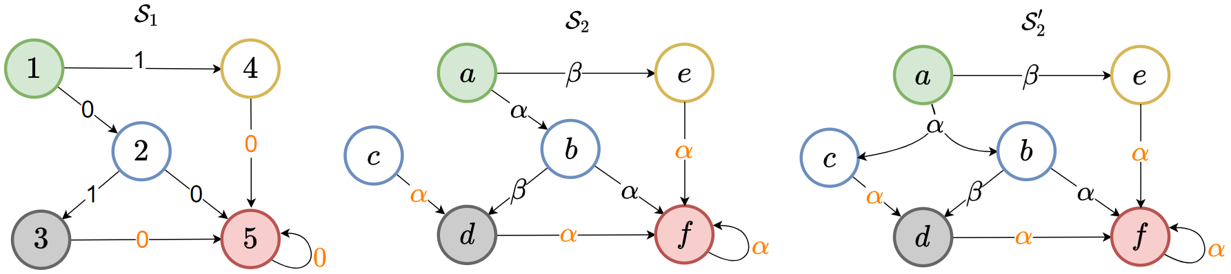
Figure 5: Three transition systems $\mathcal{S}_{1}=(\mathcal{X}_{1},\mathcal{U}_{1},F_{1})$, $\mathcal{S}_{2}=(\mathcal{X}_{2},\mathcal{U}_{2},F_{2})$ and $\mathcal{S}_{2}^{\prime}=(\mathcal{X}_{2},\mathcal{U}_{2},F_{2}^{\prime})$ and a relation $R\subseteq\mathcal{X}_{1}\times\mathcal{X}_{2}$. Specifically, $\mathcal{X}_{1}=(1,2,3,4,5)$, $\mathcal{U}_{1}=\{0,1\}$, $\mathcal{X}_{2}=(a,b,c,d,e,f)$, $\mathcal{U}_{2}=\{\alpha,\beta,\gamma\}$, the transition maps $F_{1}$, $F_{2}$ and $F_{2}^{\prime}$ and the available inputs maps $\mathcal{U}_{1}(.)$, $\mathcal{U}_{2}(.)$ and $\mathcal{U}_{2}^{\prime}(.)$ are clear from the illustration, and $R=\{(1,a),(2,b),(2,c),(3,d),(4,e),(5,f)\}$. The colors of the node indicate the related states. Inputs labeled orange simply indicate that their values are not relevant to the current discussion. We consider the concrete specification $\Sigma_{1}^{\text{Reach}}=[\{1\},\{5\},\{3\}]$ and the associated abstract specification $\Sigma_{2}^{\text{Reach}}=\Sigma_{2}^{\text{Reach}^{\prime}}=[\{a\},\{f\},\{d\}]$, where the initial, target and obstacle states are respectively in green, red and black.

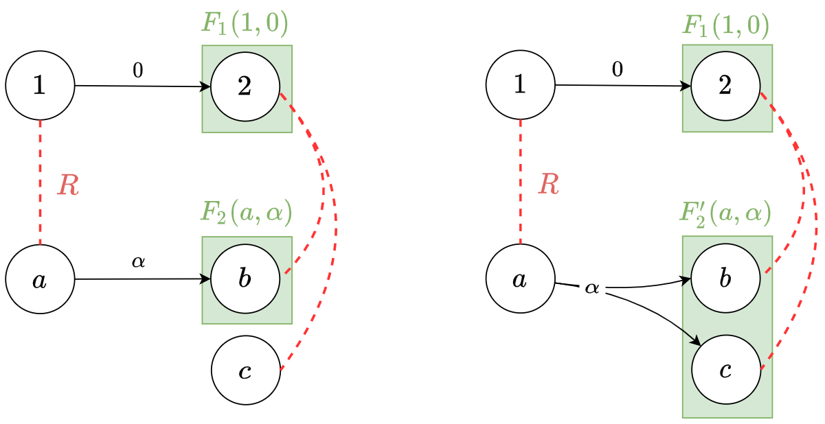
Figure 6: Local transition of two related states $(1,a)\in R$ and relation $R$ defined in Figure 5. Left: Transition for $\mathcal{S}_{2}$. Right: Transitions for $\mathcal{S}_{2}^{\prime}$.

We consider the two deterministic systems $\mathcal{S}_{1}$ and $\mathcal{S}_{2}$ given in Figure 5. One can verify from  Definition 5 that the relation $R$ is an alternating simulation relation, i.e., $\mathcal{S}_{1}\preceq_{R}^{\operatorname{ASR}}\mathcal{S}_{2}$. Note that this relation corresponds to a cover-based abstraction, since $R(2)=\{b,c\}$ is not a singleton. We consider the concrete specifications $\Sigma_{1}$ consisting in controlling $\mathcal{S}_{1}$ from the initial state $1$ to the target state $5$ while avoiding the obstacle state $3$. The associated abstract specifications $\Sigma_{2}$ consist in controlling $\mathcal{S}_{2}$ from the initial state $a$ to the target state $f$ while avoiding the obstacle state $d$. The controller $\mathcal{C}_{2}$ satisfying

$$\mathcal{C}_{2}(a)=\{\alpha\},\ \mathcal{C}_{2}(b)=\{\alpha\}$$ (7)

solves the abstract problem. The maximal interface associated to $R$ is given by

$$I_{R}^{\operatorname{ASR}}(1,a,\alpha)=\{0\},\ I_{R}^{\operatorname{ASR}}(2,b,\alpha)=\{0\},\ I_{R}^{\operatorname{ASR}}(2,c,\alpha)=\{1\}.$$

We consider the associated memoryless concretized controller, $\mathcal{C}_{1}=\mathcal{C}_{2}\circ_{I_{R}^{\operatorname{ASR}}}R$. We compute the relevant values:

$$\mathcal{C}_{1}(1)=\{0\},\ \mathcal{C}_{1}(2)=\{0,1\}.$$

We can construct the trajectory $(\bm{x}_{1},\bm{u}_{1})\in\mathcal{B}(\mathcal{C}_{1}\times\mathcal{S}_{1})$ with $\bm{x}_{1}=(1,2,3)$ and $\bm{u}_{1}=(0,1)$ which leads to a contradiction with the dynamics of $\mathcal{C}_{2}\times\mathcal{S}_{2}$ since the controlled simulability property requires the existence of an abstract trajectory $(\bm{x}_{2},\bm{u}_{2})$ such that $x_{2}(0)=a$ and $x_{2}(2)=d$. This shows that $\mathcal{C}_{1}$ does not satisfy (3). As a result, this specific controller does not offer the formal guarantee of avoiding the obstacle and reaching the target.

However, the controller $\mathcal{C}_{1}^{\prime}$ defined as

$$\mathcal{C}^{\prime}_{1}(1)=\{0\},\ \mathcal{C}^{\prime}_{1}(2)=\{0\}$$

satisfies (3) (note that its existence was guaranteed by Theorem 2, but that there was no guarantee that it was static). Indeed, the trajectory $(\bm{x}_{1}^{\prime},\bm{u}_{1}^{\prime})\in\mathcal{B}(\mathcal{C}^{\prime}_{1}\times\mathcal{S}_{1})$ with $\bm{x}_{1}^{\prime}=(1,2,5)$ and $\bm{u}_{1}^{\prime}=(0,0)$ aligns with a corresponding abstract trajectory $(\bm{x}_{2}^{\prime},\bm{u}_{2}^{\prime})\in\mathcal{B}(\mathcal{C}_{2}\times\mathcal{S}_{2})$ with $\bm{x}_{2}^{\prime}=(a,b,f)$ and $\bm{u}_{2}^{\prime}=(\alpha,\alpha)$, while the previously defined trajectory $(\bm{x}_{1},\bm{u}_{1})\notin\mathcal{B}(\mathcal{C}^{\prime}_{1}\times\mathcal{S}_{1})$.

On the other hand, if we adopt an abstract controller defined as follows

$$\tilde{\mathcal{C}}_{2}(a)=\{\beta\},\ \tilde{\mathcal{C}}_{2}(e)=\{\alpha\}$$ (8)

which also solves the abstract problem, then the controller $\tilde{\mathcal{C}}_{1}$, where $\tilde{\mathcal{C}}_{1}=\tilde{\mathcal{C}}_{2}\circ_{I_{R}^{\operatorname{ASR}}}R$ is the associated memoryless concretized controller, satisfies (3).

Nevertheless, we aim to establish conditions that guarantee that the memoryless concretized controller ensures the controlled simulability property whatever the abstract controller.

In the subsequent subsection, we will introduce a relation that is not only sufficient to ensure this specific concretization scheme but is also necessary to ensure its feasibility for every abstract controller.

IV-B Definition and properties

The crucial point in the failure of the previous example is that the $\operatorname{ASR}$ condition only imposes that for each transition from $x_{1}$ to $x_{1}^{\prime}$ in $\mathcal{S}_{1}$ there exists a state $x_{2}^{\prime}\in R(x_{1}^{\prime})$ that is a successor of $x_{2}$ in $\mathcal{S}_{2}$, but it is not required that every $x_{2}^{\prime\prime}\in R(x_{1}^{\prime})$ succeeds $x_{2}$ (note that it was the case in the previous example as illustrated in Figure 6). The relation presented below is introduced to circumvent the specific problem describe previously.

Definition 8 ($\operatorname{MCR}$).

A relation $R\subseteq\mathcal{X}_{1}\times\mathcal{X}_{2}$ is a memoryless concretization relation from $\mathcal{S}_{1}$ to $\mathcal{S}_{2}$ if for every $(x_{1},x_{2})\in R$ for every $u_{2}\in\mathcal{U}_{2}(x_{2})$ there exists $u_{1}\in\mathcal{U}_{1}(x_{1})$ such that for every $x_{1}^{\prime}\in F_{1}(x_{1},u_{1})$ for every $x_{2}^{\prime}$ such that $(x_{1}^{\prime},x_{2}^{\prime})\in R$: $x_{2}^{\prime}\in F_{2}(x_{2},u_{2})$.

The local condition stated in Definition 8 is illustrated for some $(x_{1},x_{2},u_{1},u_{2})\in R_{e}^{\operatorname{MCR}}$ in Figure 3 (right). The fact that $R$ is a memoryless concretization relation from $\mathcal{S}_{1}$ to $\mathcal{S}_{2}$ will be denoted $\mathcal{S}_{1}\preceq_{R}^{\operatorname{MCR}}\mathcal{S}_{2}$, and we write $\mathcal{S}_{1}\preceq^{\operatorname{MCR}}\mathcal{S}_{2}$ if $\mathcal{S}_{1}\preceq_{R}^{\operatorname{MCR}}\mathcal{S}_{2}$ holds for some $R$.

The memoryless concretization relation is a relaxed version of the feedback refinement relation introduced in [1, V.2 Definition]. Specifically, we relax the requirement that the concrete and abstract inputs must be identical.

Theorem 3.

Given two systems, $\mathcal{S}_{1}$ and $\mathcal{S}_{2}$, and a strict relation $R$, the following statements hold

1. If $\mathcal{S}_{1}\preceq_{R}^{\operatorname{MCR}}\mathcal{S}_{2}$, then $\mathcal{S}_{1}\preceq_{R}^{\operatorname{ASR}}\mathcal{S}_{2}$.

2. Additionally, if $R$ is single-valued (i.e., defines a partition), the converse is true.

Proof.

1. Rewriting the definition slightly, we have

   • $\operatorname{ASR}$: for every $(x_{1},x_{2})\in R$ and for every $u_{2}\in\mathcal{U}_{2}(x_{2})$ there exists $u_{1}\in\mathcal{U}_{1}(x_{1})$ such that for every $x_{1}^{\prime}\in F_{1}(x_{1},u_{1}):R(x_{1}^{\prime})\cap F_{2}(x_{2},u_{2})\neq\varnothing$.

   • $\operatorname{MCR}$: for every $(x_{1},x_{2})\in R$ and for every $u_{2}\in\mathcal{U}_{2}(x_{2})$ there exists $u_{1}\in\mathcal{U}_{1}(x_{1})$ such that for every $x_{1}^{\prime}\in F_{1}(x_{1},u_{1}):R(x_{1}^{\prime})\subseteq F_{2}(x_{2},u_{2})$.

   Since $R$ is strict, $R(x_{1}^{\prime})$ is nonempty and therefore $R(x_{1}^{\prime})\subseteq F_{2}(x_{2},u_{2})$ implies $R(x_{1}^{\prime})\cap F_{2}(x_{2},u_{2})\neq\varnothing$.

2. Given that $R$ is a strict relation and single-valued, it can be established that for any $x_{1}\in\mathcal{X}_{1}$: $|R(x_{1})|=1$. Therefore $R(x_{1}^{\prime})\cap F_{2}(x_{2},u_{2})\neq\varnothing$ if and only if $R(x_{1}^{\prime})\subseteq F_{2}(x_{2},u_{2})$.

∎

Note that the condition that the relation forms a partition is sufficient to guarantee that an $\operatorname{ASR}$ is a $\operatorname{MCR}$, but it is not a necessary condition.

We prove that $\preceq^{\operatorname{MCR}}$ is reflexive and transitive, which justifies the use of the pre-order symbol $\preceq$.

Proposition 1.

Let $\mathcal{S}_{1},\mathcal{S}_{2}$ and $\mathcal{S}_{3}$ be transition systems, and $R,Q$ be strict relations. Then

1. $\mathcal{S}_{1}\preceq_{Id_{\mathcal{X}_{1}}}^{\operatorname{MCR}}\mathcal{S}_{1}$;

2. If $\mathcal{S}_{1}\preceq_{R}^{\operatorname{MCR}}\mathcal{S}_{2}$ and $\mathcal{S}_{2}\preceq_{Q}^{\operatorname{MCR}}\mathcal{S}_{3}$, then $\mathcal{S}_{1}\preceq_{R\circ Q}^{\operatorname{MCR}}\mathcal{S}_{3}$.

Proof.

The identity relation $Id_{\mathcal{X}_{1}}$ satisfies the definition of $\operatorname{MCR}$ with $\mathcal{S}_{1}=\mathcal{S}_{2}$, $x_{1}=x_{2}$ and $u_{1}=u_{2}$, which proves (1). To prove (2), assume that $\mathcal{S}_{1}\preceq_{R}^{\operatorname{MCR}}\mathcal{S}_{2}\preceq_{Q}^{\operatorname{MCR}}\mathcal{S}_{3}$. Then $R\circ Q$ is strict since both $R$ and $Q$ are strict. Let $(x_{1},x_{3})\in R\circ Q$. Then there exists $x_{2}\in\mathcal{X}_{2}$ such that $(x_{1},x_{2})\in R$ and $(x_{2},x_{3})\in Q$. Since both $Q$ and $R$ are $\operatorname{MCR}$, then we have

$$\forall u_{3}\in\mathcal{U}_{3}(x_{3})\exists u_{2}\in\mathcal{U}_{2}(x_{2}):\ Q(F_{2}(x_{2},u_{2}))\subseteq F_{3}(x_{3},u_{3});$$

$$\forall u_{2}\in\mathcal{U}_{2}(x_{2})\exists u_{1}\in\mathcal{U}_{1}(x_{1}):\ R(F_{1}(x_{1},u_{1}))\subseteq F_{2}(x_{2},u_{2});$$

from which follows

$$\forall u_{3}\in\mathcal{U}_{3}(x_{3})\exists u_{1}\in\mathcal{U}_{1}(x_{1}):\ Q(R(F_{1}(x_{1},u_{1})))\subseteq F_{3}(x_{3},u_{3})$$

and so $\mathcal{S}_{1}\preceq_{R\circ Q}^{\operatorname{MCR}}\mathcal{S}_{3}$. ∎

Property 2 (Memoryless concretization property).

Given two systems $\mathcal{S}_{1}$ and $\mathcal{S}_{2}$, and a strict relation $R\subseteq\mathcal{X}_{1}\times\mathcal{X}_{2}$ of type $\operatorname{T}$, we say that the tuple $(\mathcal{S}_{1},\mathcal{S}_{2},R)$ satisfies the memoryless concretization property if if every controller $\mathcal{C}_{2}$

$$R(\mathcal{B}_{x}(\mathcal{C}_{1}\times\mathcal{S}_{1}))\subseteq\mathcal{B}_{x}(\mathcal{C}_{2}\times\mathcal{S}_{2})$$ (9)

with $\mathcal{C}_{1}=\mathcal{C}_{2}\circ_{I_{R}^{\operatorname{T}}}R$.

This property guarantees that the controller $\mathcal{C}_{1}=\mathcal{C}_{2}\circ_{I_{R}^{\operatorname{T}}}R$ can only generate abstract trajectories that belongs to the behavior of the system $\mathcal{C}_{2}\times\mathcal{S}_{2}$. To compare and contrast with 1, we require two different things. The first is that every quantization of a concrete trajectory is a valid abstract trajectory, as opposed to the existence of one related abstract trajectory. This is preferable if the quantizer is assumed adversarial, or alternatively, if you are free to choose the quantization that suits you best, e.g., the fastest to compute. The second thing that 2 requires is that (9) holds for a very specific controller, which gives us a straightforward implementation.

Theorem 4.

Given two transition systems $\mathcal{S}_{1}$ and $\mathcal{S}_{2}$, and a strict relation $R$, if $\mathcal{S}_{1}\preceq_{R}^{\operatorname{MCR}}\mathcal{S}_{2}$ then the tuple $(\mathcal{S}_{1},\mathcal{S}_{2},R)$ satisfies the memoryless concretization property (2).

Proof.

Consider a trajectory $(\bm{x}_{1},\bm{u}_{1})\in\mathcal{B}(\mathcal{C}_{1}\times\mathcal{S}_{1})$ of length $T$ with $\mathcal{C}_{1}=\mathcal{C}_{2}\circ_{I_{R}^{\operatorname{MCR}}}R$, i.e.,

1. $\forall k\in[0;T[:\ x_{1}(k+1)\in F_{1}(x_{1}(k),u_{1}(k))$;

2. $\forall k\in[0;T-1[:\ u_{1}(k)\in\mathcal{C}_{1}(x_{1})$.

Then by definition of $\mathcal{C}_{1}$, for any related sequence $\bm{x}_{2}$ of length $T$ such that $\forall k\in[0;T[:\ x_{2}(k)\in R(x_{1}(k))$, there exists a sequence $\bm{u}_{2}$ of length $T-1$ such that

1. $\forall k\in[0;T-1[:\ u_{2}(k)\in\mathcal{C}_{2}(x_{2}(k))$;

2. $\forall k\in[0;T-1[:\ u_{1}(k)\in I_{R}^{\operatorname{MCR}}(x_{1}(k),x_{2}(k),u_{2}(k))$.

because $\mathcal{C}_{2}$ and $I_{R}^{\operatorname{MCR}}$ are non-empty.

Our goal is to establish that $(\bm{x}_{2},\bm{u}_{2})\in\mathcal{B}(\mathcal{C}_{2}\times\mathcal{S}_{2})$, which translates to

1. $\forall k\in[0;T-1[:\ u_{2}(k)\in\mathcal{U}_{2}(x_{2}(k))$;

2. $\forall k\in[0;T-1[:\ x_{2}(k+1)\in F_{2}(x_{2}(k),u_{2}(k))$.

To prove (1”), we can directly use condition (1’). To prove (2”), taking into account condition (2’) and $\mathcal{S}_{1}\preceq_{R}^{\operatorname{MCR}}\mathcal{S}_{2}$, we can observe that

$$\forall x_{1}^{\prime}\in F_{1}(x_{1}(k),u_{1}(k)):\ (x_{1}^{\prime},x_{2}^{\prime})\in R\Rightarrow x_{2}^{\prime}\in F_{2}(x_{2}(k),u_{2}(k)).$$ (10)

Given the preceding conditions (1’), (2’), and the established implication (10), it follows that $x_{2}(k+1)\in F_{2}(x_{2}(k),u_{2}(k))$. ∎

Furthermore, the existence of a memoryless concretization relation between the concrete system and the abstraction is not only sufficient to guarantee memoryless concretization property, it is also necessary when we want it to be applicable whatever the particular specification we seek to impose on the concrete system, as established by the following theorem.

Theorem 5.

Given two systems $\mathcal{S}_{1}$ and $\mathcal{S}_{2}$, and a strict relation $R$ such that $\mathcal{S}_{1}\preceq_{R}^{\operatorname{ASR}}\mathcal{S}_{2}$, if $(\mathcal{S}_{1},\mathcal{S}_{2},R)$ satisfies the memoryless concretization property (2), then $\mathcal{S}_{1}\preceq_{R}^{\operatorname{MCR}}\mathcal{S}_{2}$.

Proof.

We proceed by contraposition. Let’s assume that $R$ does not satisfy the condition of Definition 8. This implies the existence of $(x_{1},x_{2})\in R$ and $u_{2}\in\mathcal{U}_{2}(x_{2})$ such that for every $u_{1}\in\mathcal{U}_{1}(x_{1})$, there exist $x_{1}^{\prime}\in F_{1}(x_{1},u_{1})$ and $x_{2}^{\prime}\in R(x_{1}^{\prime})$ such that $x_{2}^{\prime}\notin F_{2}(x_{2},u_{2})$. We consider an abstract controller $\mathcal{C}_{2}$ such that $\mathcal{C}_{2}(x_{2})=\{u_{2}\}$. Let $u_{1}\in I_{R}^{\operatorname{MCR}}(x_{1},x_{2},u_{2})\subseteq\mathcal{U}_{1}(x_{1})$. Let’s define the sequences $\bm{\tilde{x}}_{1}=(x_{1},x_{1}^{\prime})$, $\bm{\tilde{u}}_{1}=(u_{1})$, $\bm{\tilde{x}}_{2}=(x_{2},x_{2}^{\prime})$, and $\bm{\tilde{u}}_{2}=(u_{2})$. We observe that $(\bm{\tilde{x}}_{1},\bm{\tilde{u}}_{1})\in\mathcal{B}(\mathcal{C}_{1}\times\mathcal{S}_{1})$ with $\mathcal{C}_{1}=\mathcal{C}_{2}\circ_{I_{R}^{\operatorname{MCR}}}R$ while $(\bm{\tilde{x}}_{2},\bm{\tilde{u}}_{2})\notin\mathcal{B}(\mathcal{C}_{2}\times\mathcal{S}_{2})$ since $\tilde{x}_{2}(1)\notin F_{2}(x_{2},u_{2})$. This means that the tuple $(\mathcal{S}_{1},\mathcal{S}_{2},R)$ does not satisfy the memoryless concretization property. This concludes the proof. ∎

From any given $\operatorname{ASR}$ abstraction, it is possible to construct a $\operatorname{MCR}$ abstraction, albeit with an increase in non-determinism. This augmentation is achieved by introducing additional transitions, as formally established by the subsequent proposition.

Proposition 2.

Consider two systems $\mathcal{S}_{1}=(\mathcal{X}_{1},\mathcal{U}_{1},F_{1})$ and $\mathcal{S}_{2}=(\mathcal{X}_{2},\mathcal{U}_{2},F_{2})$ and a relation $R$ that satisfies $\mathcal{S}_{1}\preceq_{R}^{\operatorname{ASR}}\mathcal{S}_{2}$. Then the system $\mathcal{S}_{2}^{\prime}=(\mathcal{X}_{2},\mathcal{U}_{2},F_{2}^{\prime})$ such that $\forall x_{2}\in\mathcal{X}_{2}$ and $\forall u_{2}\in\mathcal{U}_{2}(x_{2})$:

1. $\mathcal{U}_{2}^{\prime}(x_{2})=\mathcal{U}_{2}(x_{2})$;

2. $F_{2}^{\prime}(x_{2},u_{2})=F_{2}(x_{2},u_{2})\cup\left(\bigcup_{(x_{1},x_{2},u_{1},u_{2})\in R_{e}^{\operatorname{ASR}}}\ R(F_{1}(x_{1},u_{1}))\right)$;

satisfies $\mathcal{S}_{2}\preceq_{Id_{\mathcal{X}_{2}}}^{\operatorname{MCR}}\mathcal{S}_{2}^{\prime}$ and $\mathcal{S}_{1}\preceq_{R}^{\operatorname{MCR}}\mathcal{S}_{2}^{\prime}$.
We call it the $\operatorname{MCR}$-extension of $\mathcal{S}_{2}$.

Proof.

The condition of Definition 8, i.e., $\forall(x_{2},x_{2})\in Id_{\mathcal{X}_{2}}$ and $\forall u_{2}^{\prime}\in\mathcal{U}_{2}^{\prime}(x_{2})$ there exists $u_{2}\in\mathcal{U}_{2}(x_{2})$ such that $F_{2}(x_{2},u_{2})\subseteq Id_{\mathcal{X}_{2}}(F_{2}^{\prime}(x_{2},u_{2}^{\prime}))$, holds by taking $u_{2}=u_{2}^{\prime}$ (by (i)), and the inclusion is ensured by (ii). This conclude the proof that $\mathcal{S}_{2}\preceq_{Id_{\mathcal{X}_{2}}}^{\operatorname{MCR}}\mathcal{S}_{2}^{\prime}$.

Since $\mathcal{S}_{1}\preceq_{R}^{\operatorname{ASR}}\mathcal{S}_{2}$ and $\mathcal{S}_{2}\preceq_{Id_{\mathcal{X}_{2}}}^{\operatorname{MCR}}\mathcal{S}_{2}^{\prime}$, by the transitivity of $\operatorname{ASR}{}$, we can easily conclude that $\mathcal{S}_{1}\preceq_{R\circ Id_{\mathcal{X}_{2}}}^{\operatorname{ASR}}\mathcal{S}_{2}^{\prime}$, which is equivalent to $\mathcal{S}_{1}\preceq_{R}^{\operatorname{ASR}{}}\mathcal{S}_{2}^{\prime}$. In addition, by (ii), the $\operatorname{MCR}$ condition, i.e., $\forall(x_{1},x_{2})\in R$ and $\forall u_{2}\in\mathcal{U}_{2}(x_{2})$, $\exists u_{1}\in\mathcal{U}_{1}(x_{1}):\ R(F_{1}(x_{1},u_{1}))\subseteq F_{2}^{\prime}(x_{2},u_{2})$, holds. This completes the proof that $\mathcal{S}_{1}\preceq_{R}^{\operatorname{MCR}}\mathcal{S}_{2}^{\prime}$. ∎

Note that condition (i) limits the addition of a transition to existing labeled transitions.

We stress that the system $\mathcal{S}_{2}^{\prime}=(\mathcal{X}_{2},\mathcal{U}_{2},F_{2}^{\prime})$ of Proposition 2 is not the only way to define a $\operatorname{MCR}$-extension of $\mathcal{S}_{2}$. We chose this definition to show existence of a $\operatorname{MCR}$-extension.

IV-C Concretization procedure

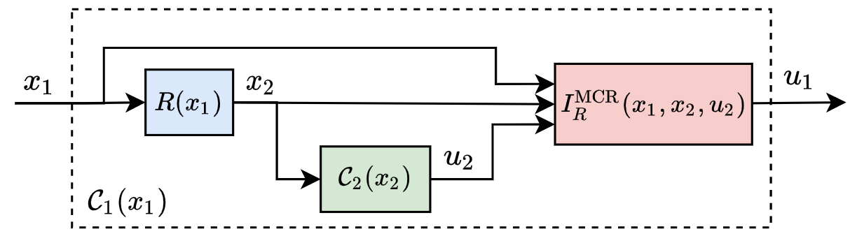
Figure 7: Memoryless concretized controller architecture $\mathcal{C}_{1}=\mathcal{C}_{2}\circ_{I_{R}^{\operatorname{MCR}}}R$ such that $(\mathcal{S}_{1},\mathcal{S}_{2},\mathcal{C}_{1},\mathcal{C}_{2},R)$ satisfies the controlled simulability property if $\mathcal{S}_{1}\preceq_{R}^{\operatorname{MCR}}\mathcal{S}_{2}$.

As already mention with the motivating example of this section, the memoryless concretization relation enables simpler concrete control architecture illustrated in Figure 7. The advantage of this control architecture is that the concrete controller only depends on the current concrete state and does not need to keep track of where the abstract system is supposed to be. In practice the abstraction is not needed once the abstract controller has been designed. Note, if the abstract controller $\mathcal{C}_{2}$ is static, then the concretized controller will be static as well.

Nevertheless, the interface $I_{R}^{\operatorname{MCR}}$ implicitly embeds the extended relation $R_{e}^{\operatorname{MCR}}$ into the concrete controller. A very convenient case is when the interface is a function for which we have an explicit characterization, as we can simply compute it as needed, removing the implementation cost of storing the extended relation. For example, consider the context of a piecewise affine controller for the concrete system, i.e., where given $x_{2}\in\mathcal{X}_{2}$ and $u_{2}\in\mathcal{C}_{2}(x_{2})$, we have $\forall x_{1}\in R^{-1}(x_{2}):\ I_{R}^{\operatorname{MCR}}(x_{1},x_{2},u_{2})=\kappa(x_{1})=\mathbf{K}x_{1}+l$. The abstract input $u_{2}\in\mathcal{C}_{2}(x_{2})$ can be interpreted as the local controller $\kappa$ for as long as we are in the cell $R^{-1}(x_{2})\subseteq\mathcal{X}_{1}$.

Let’s now return to the motivating example of this section given in Figure 5. First note that the relation $R$ is not a $\operatorname{MCR}$ for systems $\mathcal{S}_{1}$ and $\mathcal{S}_{2}$ ($\mathcal{S}_{1}\npreceq_{R}^{\operatorname{MCR}}\mathcal{S}_{2}$) due to the following observations: $(1,a)\in R$, $\alpha\in\mathcal{U}_{2}(a)$, $0\in\mathcal{U}_{1}(1)$, $2\in F_{1}(1,0)$, $c\in R(2)$ and $c\notin F_{2}(a,\alpha)$ as illustrated in Figure 6. We will now turn our attention to system $\mathcal{S}_{2}^{\prime}$ introduced in Figure 5. We can prove that $\mathcal{S}_{1}\preceq_{R}^{\operatorname{MCR}}\mathcal{S}_{2}^{\prime}$ and that, consequently, Theorem 4 guarantees that any memoryless concretized controller will satisfy the controlled simulability property. However, the gain in this property comes at the cost of an increase in non-determinism in the abstraction (note that $\mathcal{S}_{2}^{\prime}$ is the $\operatorname{MCR}$-extension of $\mathcal{S}_{2}$): whereas $\mathcal{S}_{2}$ was deterministic, $\mathcal{S}_{2}^{\prime}$ is now non-deterministic. As a result, the abstract problem is harder to solve since it is no longer a simple path-finding problem on a directed graph, but a reachability problem on a weighted directed forward hypergraph. That is, each transition corresponds to a forward hyperarc which is a hyperarc with one tail and multiple heads, see [19] for an introduction to hypergraphs. In addition, whereas the abstract problem $(\mathcal{S}_{2},\Sigma_{2})$ had two solutions, the controllers $\mathcal{C}_{2}$ given by (7) and $\mathcal{C}_{2}^{\prime}$ given by (8), the abstract problem $(\mathcal{S}_{2}^{\prime},\Sigma_{2}^{\prime})$ has only one solution, the controller $\mathcal{C}_{2}^{\prime}$. So, not only may the abstract problem $(\mathcal{S}_{2}^{\prime},\Sigma_{2}^{\prime})$ be more difficult to solve, it may also admit less or no solution at all.

IV-D Comparison between $\operatorname{MCR}$ and $\operatorname{FRR}$

As previously mentioned, the $\operatorname{MCR}$ extends to the feedback refinement relation [1, V.2 Definition], whose definition we recall.

Definition 9 ($\operatorname{FRR}$).

A relation $R\subseteq\mathcal{X}_{1}\times\mathcal{X}_{2}$ is a feedback refinement relation from $\mathcal{S}_{1}$ to $\mathcal{S}_{2}$ if for every $(x_{1},x_{2})\in~{}R$:

1. $\mathcal{U}_{2}(x_{2})\subseteq\mathcal{U}_{1}(x_{1})$;

2. for every $u\in\mathcal{U}_{2}(x_{2})$ and for every $x_{1}^{\prime}\in F_{1}(x_{1},u)$ for every $x_{2}^{\prime}$ such that $x_{2}^{\prime}\in R(x_{1}^{\prime})$: $x_{2}^{\prime}\in F_{2}(x_{2},u)$.

The fact that $R$ is a feedback refinement relation from $\mathcal{S}_{1}$ to $\mathcal{S}_{2}$ will be denoted $\mathcal{S}_{1}\preceq_{R}^{\operatorname{FRR}}\mathcal{S}_{2}$, and we write $\mathcal{S}_{1}\preceq^{\operatorname{FRR}}\mathcal{S}_{2}$ if $\mathcal{S}_{1}\preceq_{R}^{\operatorname{FRR}}\mathcal{S}_{2}$ holds for some $R$.

Proposition 3.

Given two systems $\mathcal{S}_{1}$ and $\mathcal{S}_{2}$, if $\mathcal{S}_{1}\preceq_{R}^{\operatorname{FRR}}\mathcal{S}_{2}$, then $\mathcal{S}_{1}\preceq_{R}^{\operatorname{MCR}}~{}\mathcal{S}_{2}$.

Proof.

It’s the same definition as $\operatorname{MCR}$, with the additional constraint that the abstract and concrete input in the extended relation are the same, that is to say $I_{R}^{\operatorname{MCR}}(x_{1},x_{2},u_{2})=\{u_{2}\}\subseteq\mathcal{U}_{1}(x_{1})$. ∎

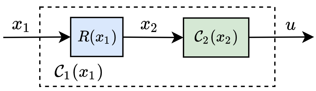
Figure 8: Memoryless concretized controller architecture $\mathcal{C}_{1}=\mathcal{C}_{2}\circ R$ for $\mathcal{S}_{1}\preceq_{R}^{\operatorname{FRR}}\mathcal{S}_{2}$.

In this case, the controller architecture in Figure 7 simplifies with $I_{R}^{\operatorname{MCR}}(x_{1},x_{2},u_{2})=\{u_{2}\}$ in the architecture given in Figure 8. The concrete controller can be rewritten as $\mathcal{C}_{1}=\mathcal{C}_{2}\circ_{I_{R}^{\operatorname{MCR}}}R=\mathcal{C}_{2}\circ R$, i.e., the functional composition of $\mathcal{C}_{2}$ and $R$ viewed as set-valued maps. This justifies the notation $\circ_{I_{R}^{\operatorname{MCR}}}$.

This concrete controller only requires the abstract (or symbolic) state, it does not need the concrete state $x_{1}$; we say that the concretization is carried out using only symbolic information. Consequently, $\operatorname{FRR}$ restricts its class of concrete controllers exclusively to piecewise constant controllers. Therefore, the feedback refinement relation is well suited to the context where the exact state is not known and only quantified (or symbolic) state information is available. On the other hand, when information on the concrete state is available, this is a major restriction, as the following example illustrates.

To motivate the use of a $\operatorname{MCR}$ versus a $\operatorname{FRR}$, we provide the following example where, for a given relation $R$ (i.e., a given discretization), we can solve the concrete problem following the three-step abstraction-based procedure described in Section I with a $\operatorname{MCR}$ whereas this is impossible with a $\operatorname{FRR}$, i.e., using only symbolic information for the concretization.

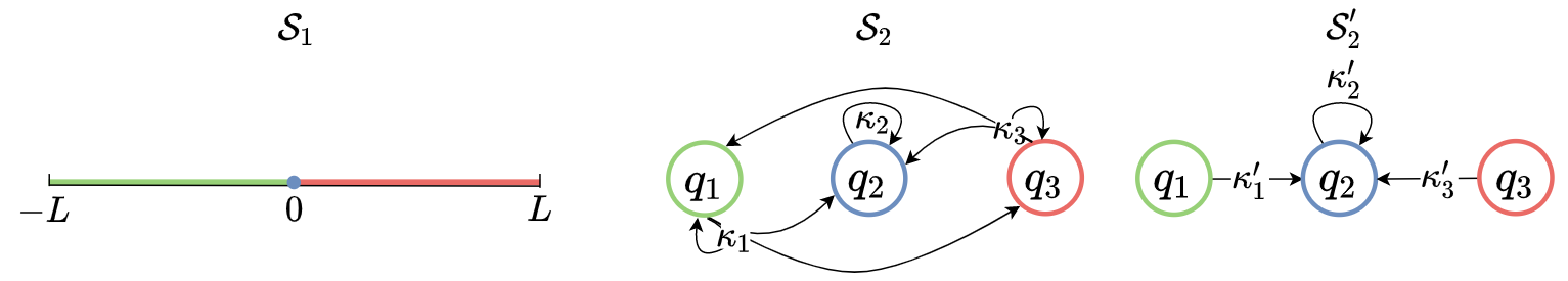
Figure 9: Three transition systems $\mathcal{S}_{1}=(\mathcal{X}_{1},\mathcal{U}_{1},F_{1})$, $\mathcal{S}_{2}=(\mathcal{X}_{2},\mathcal{U}_{2},F_{2})$, $\mathcal{S}_{2}^{\prime}=(\mathcal{X}_{2},\mathcal{U}_{2}^{\prime},F_{2}^{\prime})$ and a relation $R\subseteq\mathcal{X}_{1}\times\mathcal{X}_{2}$. Specifically, $\mathcal{X}_{1}=[-L,L]\subseteq\mathbb{R}$, $\mathcal{U}_{1}=\mathbb{R}$, $\mathcal{X}_{2}=\{q_{1},q_{2},q_{3}\}$, $\mathcal{U}_{2}=\{\kappa_{1},\kappa_{2},\kappa_{3}\}$, $\mathcal{U}_{2}^{\prime}=\{\kappa_{1}^{\prime},\kappa_{2}^{\prime},\kappa_{3}^{\prime}\}$. The transition maps $F_{2}$ and $F_{2}^{\prime}$ and the available inputs $\mathcal{U}_{2}(.)$ and $\mathcal{U}_{2}^{\prime}(.)$ are clear from the illustration. Given the function $f(x,u)=x+u$, the available inputs $\mathcal{U}_{1}(x_{1})=\{u\in\mathcal{U}_{1}\mid f(x_{1},u)\in\mathcal{X}_{1}\}$ and the transition map $F_{1}(x_{1},u)=f(x_{1},u)$. Given the sets $\mathcal{X}_{q_{1}}=[-L,0)$, $\mathcal{X}_{q_{2}}=\{0\}$ and $\mathcal{X}_{q_{3}}=(0,L]$, we define the relation $R\subseteq\mathcal{X}_{1}\times\mathcal{X}_{2}$ such that $(x_{1},q)\in R\Leftrightarrow x_{1}\in\mathcal{X}_{q}$. The colors indicate the related states. We consider the concrete specification $\Sigma_{1}^{\text{Reach}}=[\mathcal{X}_{1},\{0\},\varnothing]$ and the associated abstract specifications $\Sigma_{2}^{\text{Reach}}=\Sigma_{2}^{\text{Reach}^{\prime}}=[\mathcal{X}_{2},\{q_{2}\},\varnothing]$.

We consider the system $\mathcal{S}_{1}$ whose the dynamic consists in moving under translation on a segment of the real line, and with objective to reach $0$. The full definition of $\mathcal{S}_{1}$ is in Figure 9. Any abstraction $S_{2}$ such that $\mathcal{S}_{1}\preceq^{\operatorname{FRR}}_{R}\mathcal{S}_{2}$ is constrained to have non-determinism for the cells $q_{1}$ and $q_{3}$, as exemplified by the system $\mathcal{S}_{2}$ given in Figure 9. The problem here is that by using piecewise constant controllers for the concrete system, there will always be a portion around $0$ that overshoot its target. Indeed, we have $\kappa_{1}\in[0,L]$, $\kappa_{2}=0$ and $\kappa_{3}\in[-L,0]$, and therefore, for any admissible choice of $\kappa_{1},\kappa_{2},\kappa_{3}$, the resulting abstraction $\mathcal{S}_{2}$ is non-deterministic. As a result, the abstract problem $(\mathcal{S}_{2},\Sigma_{2})$ has no solution. However, we can build an abstraction $\mathcal{S}_{2}^{\prime}$ such that $\mathcal{S}_{1}\preceq_{R}^{\operatorname{MCR}}\mathcal{S}_{2}^{\prime}$ where $\kappa_{1}^{\prime}(x_{1})=\kappa_{3}^{\prime}(x_{1})=-x_{1}$ and $\kappa_{2}^{\prime}(x_{1})=0$ are affine controllers. Note that we have the same partition of state-space, but because we can have abstract inputs that are local state-dependent controllers instead of piecewise constant real inputs, we can solve the abstract problem $(\mathcal{S}_{2}^{\prime},\Sigma_{2}^{\prime})$. For the abstract system $\mathcal{S}_{2}^{\prime}$, the inputs $\kappa_{1}^{\prime},\kappa_{2}^{\prime}$ and $\kappa_{3}^{\prime}$ can be interpreted as move to the right cell, do not move and move to the left cell respectively.

By using all the inputs at our disposal and designing local state-dependent controllers, we can remove the non-determinism imposed by the discretization of the concrete system. This is crucial because abstraction-based control guarantees that the concrete controller successfully solves a control problem for the original system, provided that the abstract controller solves the associated abstract control problem, and it is worth noting that the level of non-determinism within the abstraction directly affects the feasibility of the abstract control problem. This example illustrates that the use of concrete state information can be beneficial to construct a practical abstraction satisfying the memoryless concretization property.

Finally, let us compare our work with another relation introduced in [7, Definition 6] as the strong alternating $\epsilon$-approximate simulation relation (denoted $S$-$\operatorname{ASR}$) which is characterized by symbolic concretization property, i.e., the existence of a concrete controller using only abstract state information. In fact, $S$-$\operatorname{ASR}$ can be derived from $\operatorname{FRR}$ by relaxing condition (2) in Definition 9 in that of $\operatorname{ASR}$, while $\operatorname{MCR}$ is obtained by relaxing condition (1) in Definition 9. Therefore, in the context of abstraction with overlapping cells, $S$-$\operatorname{ASR}$ has the same drawback as $\operatorname{ASR}$, in that it does not allow the use of the controller architecture described in Figure 8, but requires the controller architecture given in Figure 4.

V Conclusion

We have introduced memoryless concretization relation, which provides a framework that guarantees a simple control architecture, requiring only information about the current state. In addition, this concretization procedure is independent of the type of dynamical systems and specifications under consideration. In particular, if the abstract controller is static, the concrete controller will also be static. We have additionally provided a precise characterization of this relation with a necessary and sufficient condition on the concretization architecture.

We have demonstrated that any alternating simulation relation can be extended to a memoryless concretization relation at the price of introducing additional non-determinism. Furthermore, we prove that $\operatorname{ASR}$ and $\operatorname{MCR}$ coincide in the particular case of a deterministic quantizer, and thus that $\operatorname{ASR}$ benefits from the memoryless concretization property in this specific case.

In addition, we showed that this framework allows the use of overlapping cells (referred to as cover-based abstraction) and piecewise state-dependent controllers, enabling the design of low-level controllers within cells, in combination with high-level abstraction-based controllers. This opens up new possibilities when co-creating the abstraction and the controller, as is done in so-called lazy abstractions.

References

- [1] G. Reissig, A. Weber, and M. Rungger, “Feedback refinement relations for the synthesis of symbolic controllers,” IEEE Transactions on Automatic Control, vol. 62, no. 4, pp. 1781–1796, 2016.
- [2] C. Belta, B. Yordanov, and E. A. Gol, Formal methods for discrete-time dynamical systems. Springer, 2017, vol. 89.
- [3] O. Kupferman and M. Y. Vardi, “Model checking of safety properties,” Formal methods in system design, vol. 19, pp. 291–314, 2001.
- [4] R. Alur, T. A. Henzinger, O. Kupferman, and M. Y. Vardi, “Alternating refinement relations,” in CONCUR’98 Concurrency Theory: 9th International Conference Nice, France, September 8–11, 1998 Proceedings 9. Springer, 1998, pp. 163–178.
- [5] P. Tabuada, Verification and control of hybrid systems: a symbolic approach. Springer Science & Business Media, 2009.
- [6] M. Rungger and M. Zamani, “Scots: A tool for the synthesis of symbolic controllers,” in Proceedings of the 19th international conference on hybrid systems: Computation and control, 2016, pp. 99–104.
- [7] A. Borri, G. Pola, and M. D. Di Benedetto, “Design of symbolic controllers for networked control systems,” IEEE Transactions on Automatic Control, vol. 64, no. 3, pp. 1034–1046, 2018.
- [8] L. N. Egidio, T. A. Lima, and R. M. Jungers, “State-feedback abstractions for optimal control of piecewise-affine systems,” in 2022 IEEE 61st Conference on Decision and Control (CDC), 2022, pp. 7455–7460.
- [9] R. Majumdar, N. Ozay, and A.-K. Schmuck, “On abstraction-based controller design with output feedback,” in Proceedings of the 23rd International Conference on Hybrid Systems: Computation and Control, 2020, pp. 1–11.
- [10] A. Girard, “Controller synthesis for safety and reachability via approximate bisimulation,” Automatica, vol. 48, no. 5, pp. 947–953, 2012.
- [11] E. Dallal, A. Colombo, D. Del Vecchio, and S. Lafortune, “Supervisory control for collision avoidance in vehicular networks with imperfect measurements,” in 52nd IEEE Conference on Decision and Control. IEEE, 2013, pp. 6298–6303.
- [12] L. Grune and O. Junge, “Approximately optimal nonlinear stabilization with preservation of the lyapunov function property,” in 2007 46th IEEE Conference on Decision and Control. IEEE, 2007, pp. 702–707.
- [13] K. Hsu, R. Majumdar, K. Mallik, and A.-K. Schmuck, “Lazy abstraction-based control for safety specifications,” in 2018 IEEE Conference on Decision and Control (CDC). IEEE, 2018, pp. 4902–4907.
- [14] B. Yordanov, J. Tumova, I. Cerna, J. Barnat, and C. Belta, “Temporal logic control of discrete-time piecewise affine systems,” IEEE Transactions on Automatic Control, vol. 57, no. 6, pp. 1491–1504, 2011.
- [15] A. Girard, “Low-complexity quantized switching controllers using approximate bisimulation,” Nonlinear Analysis: Hybrid Systems, vol. 10, pp. 34–44, 2013.
- [16] K. Hsu, R. Majumdar, K. Mallik, and A.-K. Schmuck, “Lazy abstraction-based controller synthesis,” in International Symposium on Automated Technology for Verification and Analysis. Springer, 2019, pp. 23–47.
- [17] B. Legat, R. M. Jungers, and J. Bouchat, “Abstraction-based branch and bound approach to q-learning for hybrid optimal control,” in Learning for Dynamics and Control. PMLR, 2021, pp. 263–274.
- [18] J. Calbert, B. Legat, L. N. Egidio, and R. Jungers, “Alternating simulation on hierarchical abstractions,” in IEEE Conference on Decision and Control (CDC), 2021, pp. 593–598.
- [19] G. Gallo, G. Longo, S. Pallottino, and S. Nguyen, “Directed hypergraphs and applications,” Discrete applied mathematics, vol. 42, no. 2-3, pp. 177–201, 1993.