Efficient Tensor Networks for Control-Enhanced Quantum Metrology

Abstract

We propose efficient tensor network algorithms for optimizing control-enhanced sequential strategies in estimating a large number of quantum channels, with no ancilla or bounded ancilla. Our first approach allows for applying $N-1$ arbitrary interleaved control operations between the $N$ channels to estimate, and the second approach restricts all control operations to be identical, which could further facilitate simpler experimental demonstration. The numerical experiments show that our algorithm has a good performance in optimizing the metrological protocol for $N=100$ single-qubit and two-qubit channels. In particular, our algorithm identifies a strategy that can outperform the asymptotically optimal quantum error correction protocol when $N$ is finite but large.

I Introduction

Quantum metrology [1, 2, 3] can boost the estimation precision by exploiting quantum resources. Identification of optimal strategies for large-scale quantum metrology, however, is a daunting task suffering from the curse of dimensionality. Such challenges, for example, arise in estimating physical parameters encoded in many-body quantum systems [4, 5, 6] or many copies of an unknown quantum channel [7, 8, 9, 10, 11, 12, 13]. In this work we focus on the quantum channel estimation problem.

It is a long-standing problem that, given $N$ copies of a quantum channel $\mathcal{E}_{\theta}$ carrying the parameter of interest $\theta$, what is the ultimate precision limit for estimating $\theta$ and how one could identify the optimal strategy that achieves the highest precision. For single-parameter estimation, precision bounds attainable by quantum error correction (QEC) [14, 15, 12] are known in the asymptotic limit ($N\rightarrow\infty$) and numerical algorithms for optimal strategies [16, 17] have been designed for small $N$ (e.g., $N\leq 5$). These results, however, are under the assumption that unbounded ancilla is available. Meanwhile, little is known about the metrological performance for a large but finite $N$. On the other hand, in real-world experiments, quantum channel estimation for larger $N$ with no or limited ancilla (for example, $N=8$ in Ref. [18]) can be demonstrated with identical-control-enhanced sequential use of quantum channels [18, 19]. Obviously, a gap exists between the theoretical results and the experimental requirement. The reason is that we lack an efficient way to tackle such problems for large $N$.

A fruitful approach to the classical optimization of large-scale quantum problems, mainly in many-body physics, is the tensor network formalism [20, 21]. Tensor networks provide an efficient way to classically store and extract certain relevant information of quantum systems with limited many-body entanglement. In particular, this formalism has been used in quantum metrology for many-body systems to optimize the estimation precision and the corresponding input probe state [6].

It is natural to ask whether tensor networks can be used for optimizing a sequential strategy, where $N$ channels can be applied one after another, with interleaved control operations. This is possible by our intuition, as the power of tensor networks for addressing the spatial complexity is similarly applicable for handling the temporal complexity. For example, tensor networks have been used for quantum process tomography [22] and machine learning of non-Markovian processes [23].

In this work, we develop an efficient tensor network approach to optimizing control-enhanced sequential strategies for quantum channel estimation with bounded memory (see Fig. 1). We design two algorithms based on tensor networks, for applying arbitrary control operations and identical control operations, respectively. Formulating the problem fully within the matrix product operator (MPO) formalism, we apply the alternating optimization iteratively. The computational complexity for each round of the optimization is $O(N^{2})$, where the input state and the $N-1$ control operations are updated in each round. Empiricially, the algorithm converges well after dozens of rounds. Our approach can efficiently optimize the estimation of $100$ single-qubit and two-qubit channels, and outperform the state-of-the-art asymptotically optimal QEC approach [14, 15, 12] for a finite $N$.

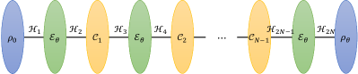
(a) Arbitrary control.

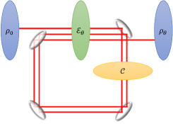
(b) Identical control ($N=3$).

Figure 1: Control-enhanced sequential strategy for estimating $\theta$ from $N$ channels $\mathcal{E}_{\theta}$, by interleaving $N-1$ control operations. Each control operation $\mathcal{C}_{i}$ for $i=1,\dots,N-1$ can be an arbitrary quantum channel (CPTP map). We can alternatively require all the control operations to be identical $\mathcal{C}_{i}=\mathcal{C}$, facilitating simpler experimental demonstration as in (b), taking $N=3$ with two identical control operations for an example. Note that this formalism also applies to the scenario with bounded ancilla, via replacing $\mathcal{E}_{\theta}$ by $\mathcal{E}_{\theta}\otimes\mathcal{I}_{A}$.

II Framework

We start with some notations. We denote by $\mathcal{L}(\mathcal{H})$ the set of linear operators on a finite-dimensional Hilbert space $\mathcal{H}$, and $\mathcal{L}[\mathcal{L}(\mathcal{H}_{1}),\mathcal{L}(\mathcal{H}_{2})]$ is the set of linear maps from $\mathcal{L}(\mathcal{H}_{1})$ to $\mathcal{L}(\mathcal{H}_{2})$. For a positive semidefinite operator $A$, we simply write $A\geq 0$.

II.1 Optimizing quantum Fisher information

A fundamental task in quantum metrology is to attain the ultimate precision limit of estimating some parameter $\theta$, given many copies of a parametrized quantum state $\rho_{\theta}\in\mathcal{L}(\mathcal{H})$. It is well known that the mean squared error (MSE) $\delta\theta^{2}$ for an unbiased estimator is bounded by the quantum Cramér-Rao bound (QCRB) [24, 25, 26]

$$\delta\theta^{2}\geq\frac{1}{\nu F^{Q}(\rho_{\theta})},$$ (1)

where $F^{Q}(\rho_{\theta})$ is the QFI and $\nu$ is the number of measurements that can be repeated. Importantly, the Cramér-Rao bound is achievable for single-parameter estimation in the limit of $\nu\rightarrow\infty$. Therefore, the QFI is a key figure of merit in quantum metrology, and it is desirable to identify an optimal strategy that is most sensitive to the parameter acquisition and thus yields an output state $\rho_{\theta}$ that maximizes the QFI.

The problem formulation in this work can be illustrated in Fig. 1. Given $N$ copies of a parametrized quantum channel $\mathcal{E}_{\theta}$, we would like to maximize the QFI of the output state $\rho_{\theta}$, by preparing an input state $\rho_{0}$ and inserting a sequence of control operations $\{\mathcal{C}_{i}\}_{i=1}^{N-1}$, where each $\mathcal{C}_{i}$ is a completely positive trace-preserving (CPTP) map. Each $\mathcal{E}_{\theta}\in\mathcal{L}[\mathcal{L}(\mathcal{H}_{2i-1}),\mathcal{L}(\mathcal{H}_{2i})]$ , for $i=1,\dots,N$, and each $\mathcal{C}_{i}\in\mathcal{L}[\mathcal{L}(\mathcal{H}_{2i}),\mathcal{L}(\mathcal{H}_{2i+1})]$, for $i=1,\dots,N-1$. For simplicity, we assume that the dimension of any $\mathcal{H}_{i}$ is the same $d=\mathsf{dim}(\mathcal{H}_{i})$. We then have the output state

$$\rho_{\theta}=\Lambda_{\theta}(\rho_{0})=\mathcal{E}_{\theta}\circ\mathcal{C}_{N-1}\circ\cdots\circ\mathcal{C}_{2}\circ\mathcal{E}_{\theta}\circ\mathcal{C}_{1}\circ\mathcal{E}_{\theta}(\rho_{0}).$$ (2)

An optimal strategy is therefore a choice of $\rho_{0}$ and $\{\mathcal{C}_{i}\}$ such that the QFI $F^{Q}(\rho_{\theta})$ is maximal. We assume that no ancilla is used in Fig. 1, but this formulation also applies to the case where an ancilla space of fixed dimension is available, as one can replace $\mathcal{E}_{\theta}$ by $\mathcal{E}_{\theta}\otimes\mathcal{I}_{A}$ in the formulation (where $A$ denotes the ancilla space).

By definition, the QFI of a state $\rho_{\theta}$ is given by $F^{Q}(\rho_{\theta})=\Tr(\rho_{\theta}L_{\theta}^{2})$, where the symmetric logarithmic derivative (SLD) $L_{\theta}$ is the solution to $2\dot{\rho}_{\theta}=\rho_{\theta}L_{\theta}+L_{\theta}\rho_{\theta}$, having denoted the derivative of $X$ with respect to $\theta$ by $\dot{X}$. Computing the QFI by this definition, however, is often challenging when the optimization of metrological strategies is concerned. Instead, we can express the QFI $F^{Q}(\rho_{\theta})$ as such a maximization problem [27, 28]:

$$F^{Q}(\rho_{\theta})=\sup_{X}\left[2\Tr(\dot{\rho_{\theta}}X)-\Tr(\rho_{\theta}X^{2})\right],$$ (3)

where $X$ is a Hermitian operator. One can check that the optimal solution for $X$ is exactly the SLD $L_{\theta}$. By combining Eq. (2), the maximal QFI obtained from $N$ channels $\mathcal{E}_{\theta}$ is given by a multivariate maximization:

$$F^{(N)}(\mathcal{E}_{\theta})=\sup_{\rho_{0},\{\mathcal{C}_{i}\}}F^{Q}(\rho_{\theta})=\sup_{\rho_{0},\{\mathcal{C}_{i}\},X}\left[2\Tr(\dot{\Lambda}_{\theta}(\rho_{0})X)-\Tr(\Lambda_{\theta}(\rho_{0})X^{2})\right].$$ (4)

Finding a global maximum for Eq. (4) can be a dauting task. However, considering that $-F^{(N)}(\mathcal{E}_{\theta})$ is a convex function of each variable in $\{\rho_{0},\{\mathcal{C}_{i}\},X\}$ while other variables are fixed, in practice we could use an alternating optimization method: we search for an optimal solution for each variable by convex optimization, while keeping the other variables fixed, and iteratively repeat the procedure for optimizing all variables in many rounds. We remark that similar ideas have also been used for optimizing metrological strategies in many-body systems [6] or with noisy measurements [29]. To implement the optimization in an efficient way for fairly large $N$, we will introduce the matrix product operator (MPO) formalism in Section II.3.

II.2 Choi operator formalism

To facilitate the mapping of the optimization problem Eq. (4) into a tensor network, we first work on the quantum comb formalism [30, 31, 32] and characterize the quantum states and multi-step quantum processes by Choi operators [33] in a unified fashion. The Choi operator of a quantum state $\rho$ is still $\rho$ itself, and the Choi operator of a quantum channel $\mathcal{E}\in\mathcal{L}[\mathcal{L}(\mathcal{H}_{\mathrm{in}}),\mathcal{L}(\mathcal{H}_{\mathrm{out}})]$ is a positive semidefinite operator in $\mathcal{L}(\mathcal{H}_{\mathrm{out}}\otimes\mathcal{H}_{\mathrm{in}})$

$$E=\mathsf{Choi}(\mathcal{E})=\mathcal{E}\otimes\mathcal{I}(\lvert I\rrangle\llangle I\rvert),$$ (5)

where $\lvert I\rrangle=\sum_{i}\ket{i}\ket{i}$ is an unnormalized maximally entangled state and $\{\ket{i}\}_{i}$ is a computational basis of $\mathcal{H}_{\mathrm{in}}$. One can easily check that $\Tr_{\mathrm{out}}E=I_{\mathrm{in}}$. $\mathcal{H}_{\mathrm{in}}$ and $\mathcal{H}_{\mathrm{out}}$ can take multiple input-output pairs of a certain causal order, corresponding to a multi-step quantum process. The composition of quantum processes $\mathcal{A}$ and $\mathcal{B}$ is then characterized by the link product [31, 32] of Choi operators $A\in\mathcal{L}\left(\otimes_{a\in\mathcal{A}}\mathcal{H}_{a}\right)$ and $B\in\mathcal{L}\left(\otimes_{b\in\mathcal{B}}\mathcal{H}_{b}\right)$, defined by

$$A*B:=\Tr_{\mathcal{A}\cap\mathcal{B}}\left[\left(I_{\mathcal{B}\backslash\mathcal{A}}\otimes A^{T_{\mathcal{A}\cap\mathcal{B}}}\right)\left(B\otimes I_{\mathcal{A}\backslash\mathcal{B}}\right)\right],$$ (6)

where $T_{i}$ denotes the partial transpose on $\mathcal{H}_{i}$, and $\mathcal{H}_{\mathcal{A}/\mathcal{B}}$ denotes $\otimes_{i\in\mathcal{A}/\mathcal{B}}\mathcal{H}_{i}$.

With the Choi-Jamiołkowski isomorphism, we denote the Choi operators of $\mathcal{E}_{\theta}\in\mathcal{L}[\mathcal{L}(\mathcal{H}_{2i-1}),\mathcal{L}(\mathcal{H}_{2i})]$ and $\mathcal{C}_{i}\in\mathcal{L}[\mathcal{L}(\mathcal{H}_{2i}),\mathcal{L}(\mathcal{H}_{2i+1})]$ by $E_{\theta}:=\mathsf{Choi}(\mathcal{E}_{\theta})$ and $C_{i}:=\mathsf{Choi}(\mathcal{C}_{i})$. Now we can reformulate Eq. (4) as

$$F^{(N)}(\mathcal{E}_{\theta})=\sup_{\rho_{0},\{C_{i}\},X}\left\{2\Tr\left[\left(\frac{dE_{\theta}^{\otimes N}}{d\theta}*\bigotimes_{i=1}^{N-1}C_{i}\otimes\rho_{0}\right)X\right]-\Tr\left[\left(E_{\theta}^{\otimes N}*\bigotimes_{i=1}^{N-1}C_{i}\otimes\rho_{0}\right)X^{2}\right]\right\},$$ (7)

where $\rho_{0}\geq 0$, $\Tr(\rho_{0})=1$, $C_{i}\geq 0$, and $\Tr_{2i+1}C_{i}=I_{2i}$ for any $i=1,\dots,N$. For ease of notation we define

$$f_{1}:=\Tr\left[\left(\frac{dE_{\theta}^{\otimes N}}{d\theta}*\bigotimes_{i=1}^{N-1}C_{i}\otimes\rho_{0}\right)X\right]$$ (8)

and

$$f_{2}:=\Tr\left[\left(E_{\theta}^{\otimes N}*\bigotimes_{i=1}^{N-1}C_{i}\otimes\rho_{0}\right)X^{2}\right].$$ (9)

A main advantage of working on Choi operators is that, it facilitates the optimization of each variable in $\{\rho_{0},\{C_{i}\},X\}$. While other variables are fixed in the alternating optimization, the optimal solution for each variable in a convex set can be identified either by simple diagonalization or by semidefinite programming (SDP), as we will see later. A naive implementation of the optimization, however, concerns a Hilbert space whose dimension exponentially grows with $N$. It is essential to compute and optimize $2f_{1}-f_{2}$ efficiently in a tensor network formalism, where all matrices we need to deal with are in the form of matrix product operators.

II.3 Matrix product operators for efficient optimization

MPO is an efficient way to store and manipulate a high-dimensional matrix/tensor. As a simple example, if we would like to store the information of $E_{\theta}^{\otimes N}$ (where each $E_{\theta}$ is a $d^{2}\times d^{2}$ matrix), we do not need to explicitly store a $d^{2N}\times d^{2N}$ matrix. Instead, it is only necessary to store the information of $E_{\theta}$, so that we can retrieve each component of $E_{\theta}^{\otimes N}$ efficiently. To be more specific, we write

$$E_{\theta}=\sum_{\alpha_{2i}\alpha_{2i-1}\beta_{2i}\beta_{2i-1}}(E_{\theta})^{\alpha_{2i}\alpha_{2i-1}}_{\beta_{2i}\beta_{2i-1}}\outerproduct{\alpha_{2i}\alpha_{2i-1}}{\beta_{2i}\beta_{2i-1}},$$ (10)

which is an operator in $\mathcal{L}(\mathcal{H}_{2i}\otimes\mathcal{H}_{2i-1})$. We can thus retrieve any component $(E_{\theta}^{\otimes N})^{\alpha_{2N}\dots\alpha_{2}\alpha_{1}}_{\beta_{2N}\dots\beta_{2}\beta_{1}}$ efficiently with $O(N)$ complexity, by calculating a product $(E_{\theta})^{\alpha_{2N}\alpha_{2N-1}}_{\beta_{2N}\beta_{2N-1}}\cdots(E_{\theta})^{\alpha_{2}\alpha_{1}}_{\beta_{2}\beta_{1}}$.

The power of MPO is definitely not limited to this simple case. In fact, we will see that we can evaluate and optimize $f_{1}$ and $f_{2}$ (and thus the QFI) in the MPO formalism. First, $f_{2}$ defined by Eq. (9) is expressed as

$$f_{2}=(X^{2})^{\beta_{2N}}_{\alpha_{2N}}(E_{\theta})^{\alpha_{2N}\alpha_{2N-1}}_{\beta_{2N}\beta_{2N-1}}\cdots(C_{1})^{\alpha_{3}\alpha_{2}}_{\beta_{3}\beta_{2}}(E_{\theta})^{\alpha_{2}\alpha_{1}}_{\beta_{2}\beta_{1}}(\rho_{0})^{\alpha_{1}}_{\beta_{1}}$$ (11)

This can be schematically illustrated in Fig. 2(a). Each leg represents an index, and a connected line represents a summation over the corresponding index. Computing $f_{1}$ requires $O(N)$ complexity.

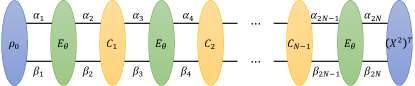
(a) Tensor network for $f_{2}$.

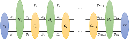
(b) Tensor network for $f_{1}$.

Figure 2: Tensor networks for computing $f_{2}$ in Eq. (9) and $f_{1}$ in Eq. (8) for evaluating the QFI. In (b), $M_{1},\dots,M_{N}$ are matrices containing the information about both $E_{\theta}$ and $\dot{E}_{\theta}$.

Computing $f_{1}$ given by Eq. (8) is a bit more involved, as the derivative $dE_{\theta}^{\otimes N}/d\theta$ needs to be evaluated. One may simply use $dE_{\theta}^{\otimes N}/d\theta=\sum_{i=1}^{N}E_{\theta}^{\otimes i-1}\otimes\dot{E}_{\theta}\otimes E_{\theta}^{\otimes N-i}$, but this introduces an $O(N^{2})$ computational overhead, which is unfavorable when $N$ is large. To circumvent this problem, we draw a technique for expressing a sum of local terms as an MPO [34, 35, 36] from many-body Hamiltonian representation. In Appendix A we show that $dE_{\theta}^{\otimes N}/d\theta$ can be written as an MPO with a bond dimension (corresponding to the $\gamma$ label) of $2$:

$$\frac{dE_{\theta}^{\otimes N}}{d\theta}=(M_{N})^{\alpha_{2N}\alpha_{2N-1}}_{\beta_{2N}\beta_{2N-1}\gamma_{N-1}}\cdots(M_{2})^{\alpha_{4}\alpha_{3}}_{\beta_{4}\beta_{3}\gamma_{2}\gamma_{1}}(M_{1})^{\alpha_{2}\alpha_{1}}_{\beta_{2}\beta_{1}\gamma_{1}},$$ (12)

where (for simplicity, we only explicitly focus on the $\gamma$ indices for the two-dimensional bond connecting $M_{1},\dots,M_{N}$)

$$(M_{N})_{1} =(M_{1})_{2}=E_{\theta},\ (M_{N})_{2}=(M_{1})_{1}=\dot{E}_{\theta},\ (M_{i}),$$ (13)

$$(M_{i})_{11} =E_{\theta},\ (M_{i})_{12}=\dot{E}_{\theta},\ (M_{i})_{21}=0,\ (M_{i})_{22}=E_{\theta},\ \forall i=2,\dots,N-1.$$

With the MPO representation of $E_{\theta}^{\otimes N}/d\theta$, we can easily see that $f_{1}$ can be computed as the contraction of a a tensor network with $O(N)$ complexity at a small cost of bond dimension of $2$, schematically illustrated in Fig. (2(b)).

The efficiency of a tensor network largely depends on the contraction order of indices. The key idea is to leave open legs as few as possible during the contraction. For our purpose this is simple: we can follow a quantum circuit time flow order (or the reverse order), and the number of open legs would not accumulate. A more detailed complexity analysis of tensor contractions during the optimization will be given in Section II.4.

II.4 Optimization procedure

With the tensor networks for $f_{1}$ and $f_{2}$, we can now efficiently optimize the QFI $F^{(N)}(\mathcal{E}_{\theta})=\sup_{\rho_{0},\{C_{i}\},X}(2f_{1}-f_{2})$ by alternating optimization.

We start with an initialization of the input state $\rho_{0}$ and the control operations $\{C_{i}\}$. The initialization can be random, or we can start from a previously known protocol which has a relatively good performance. We can use the tensor network for $f_{2}$ without the last tensor $(X^{2})^{T}$ [denoted by $f_{2}\backslash(X^{2})^{T}$] to compute the output state $\rho_{\theta}$, and use the tensor network for $f_{1}$ without the last tensor $X^{T}$ (denoted by $f_{1}\backslash X^{T}$) to compute the derivative $\dot{\rho}_{\theta}$. We then calculate the SLD of the output state [26]

$$L_{\theta}=\sum_{jk}\frac{2\matrixelement{j}{\dot{\rho}_{\theta}}{k}}{\matrixelement{j}{\rho_{\theta}}{j}+\matrixelement{k}{\rho_{\theta}}{k}}\outerproduct{j}{k},$$ (14)

where $\rho_{\theta}=\sum_{j}\matrixelement{j}{\rho_{\theta}}{j}\outerproduct{j}{j}$. Then $L_{\theta}$ is the solution for the optimal value of $X$ so far.

Now to update the input state $\rho_{0}$, we contract the tensor network $f_{2}$ without the first tensor $\rho_{0}$ (denoted by $f_{1}\backslash\rho_{0}$). Similarly, we compute $f_{2}\backslash\rho_{0}$. The updated $\rho_{0}^{\prime}$ can be identified as $\rho_{0}^{\prime}=\outerproduct{\psi_{0}^{\prime}}{\psi_{0}^{\prime}}$, where $\ket{\psi_{0}^{\prime}}$ is a normalized eigenvector of $(2f_{1}\backslash\rho_{0}-f_{2}\backslash\rho_{0})^{T}$ associated with the maximal eigenvalue. Due to the convexity of QFI, the optimal input state can always be chosen as a pure state.

For each control operation $C_{i}$, we contract $f_{1}\backslash C_{i}$ and $f_{2}\backslash C_{i}$ (with all the tensors updated so far), and compute $2f_{1}\backslash C_{i}-f_{2}\backslash C_{i}$. Without loss of generality, let us take $C_{1}$ for example. The optimization of $C_{1}$ can be formulated as an SDP:

$$\max_{C_{1}}\left[(C_{1})^{\alpha_{3}\alpha_{2}}_{\beta_{3}\beta_{2}}(2f_{1}\backslash C_{1}-f_{2}\backslash C_{1})^{\alpha_{3}\alpha_{2}}_{\beta_{3}\beta_{2}}\right],\quad\mathrm{s.t.}\ C_{1}\geq 0,\Tr_{3}C_{1}=I_{2}.$$ (15)

We can apply similar optimization for $C_{2},\dots,C_{N-1}$. It is important that each $C_{i}$ is updated by locally solving an optimization problem to circumvent the exponential overhead of a global optimization. Such an optimization procedure is motivated by the well-known algorithm for solving ground states of many-body Hamiltonians via the density matrix renormalization group (DMRG) [37, 38], wherein not an MPO representation of control operations but a matrix product state is locally updated.

We can repeat the procedure above iteratively in an outer loop of optimizing $X,\rho_{0},\{C_{i}\}$, until the required convergence is satisfied. Then we have both the optimized QFI $2f_{1}-f_{2}$ and a concrete strategy to attain it, including a probe state and a set of control operations.

We conclude this section with a complexity analysis of the tensor contraction in each round of the optimization. Assume that $\mathcal{E}_{\theta}$ acts on a $d$-dimensional system. To update $\{X,\rho_{0},\{C_{i}\}\}$, we need to contract the tensor network $O(N)$ times. Each contraction for updating a variable requires $O(Nd^{4})$ operations by sequentially following a quantum circuit order or the reverse order. Therefore, each round of the optimization requires $O(N^{2}d^{4})$ operations. In numerical experiments, we observe that the algorithm typically converges well in dozens of rounds. We remark that in practice, the computational complexity can be even lower, by storing some intermediate results of previous contractions in the memory and reusing them in a new contraction. This can be automatically implemented by the Python package opt_einsum [39] with sharing intermediates.

II.5 Alternative approach: using identical control operations

In many practical scenarios, for example, for quantum sensors with limited programmability, it is favorable to apply the same control operation at each step. To this end, we propose an alternative approach to optimizing the control operations which are required to be identical, inspired by the infinite MPO (iMPO) [35, 40, 41]. Similar techniques have been used in Ref. [6] for quantum metrology of many-body systems of infinite size. Note that in this work we employ this technique for finding identical control operations for a finite $N$.

To this end, we need to initialize all the control operations $C_{i}=C$ which are identical. With a little abuse of the notation, we denote by $2f_{1}(C)-f_{2}(C)$ the contraction result of $2f_{1}-f_{2}$ with identical control operations $C_{i}=C$. In each iteration step, we pick a control operation $C_{i}$ at random (for example, $C_{1}$) and still need to solve an SDP as in Eq. (15). The optimal solution is denoted by $\tilde{C}_{i}$. Instead of directly choosing $\tilde{C}_{i}$ to be the updated control, we take a convex combination

$$C_{i}^{\prime}(\lambda)=\sin^{2}(\lambda\pi)\tilde{C}_{i}+\cos^{2}(\lambda\pi)C_{i},$$ (16)

for some $\lambda\in[0,0.5]$ and perform the following scheme [41] to optimize $\lambda$:

1. Compute $2f_{1}(\tilde{C}_{i})-f_{2}(\tilde{C}_{i})$.

2. If $2f_{1}(\tilde{C}_{i})-f_{2}(\tilde{C}_{i})\geq 2f_{1}(C_{i})-f_{2}(C_{i})$, choose $\lambda=0.5$ and return $C_{i}^{\prime}(\lambda)=\tilde{C}_{i}$.

3. Define a larger initial step size $\delta_{0}$ (for example, $\delta_{0}=0.1$) and a smaller step size $h$ (for example, $h=10^{-4}$).

4. If $2f_{1}[C_{i}^{\prime}(h)]-f_{2}[C_{i}^{\prime}(h)]<2f_{1}(C_{i})-f_{2}(C_{i})$, choose $\lambda=0$ and return $C_{i}^{\prime}(\lambda)=C_{i}$.

5. For $i=1,\dots,T$, where $T$ is the maximal iteration,

   1. If $2f_{1}[C_{i}^{\prime}(\delta_{0})]-f_{2}[C_{i}^{\prime}(\delta_{0})]\geq 2f_{1}(C_{i})-f_{2}(C_{i})$, choose $\lambda=\delta_{0}$ and return $C_{i}^{\prime}(\lambda)$.

   2. Else, assign $\delta_{0}=\delta_{0}/2$.

This empirical method does not ensure that an optimal $C_{i}^{\prime}(\lambda)$ can be found in each iteration, and may be less robust compared to the first optimization approach without the constraint of identical control. However, in practice we note that this method performs very well in some scenarios, and this identical control algorithm often runs much faster for large $N$ (e.g., $N\approx 100$), since it does not require the optimization of all control operations separately.

III Applications

In this section, we apply the two algorithms introduced above (using arbitrary or identical control operations) to different noise models for $N=2$ to $N=100$ quantum channels, and show that our algorithm can outperform the state-of-the-art (asymptotically optimal) quantum error correction (QEC) approach [14, 15, 12] when $N$ is finite. Note that in this work we take the convention that signal comes after noise as in Ref. [13], which is more interesting in some scenarios, where the Heisenberg limit can be achieved in noisy channel estimation, but the coefficient of the scaling is smaller than the noiseless case.

We set the maximal iteration step as $50$ in the numerical experiments, when the algorithm already converges well. To achieve a faster convergence, we initialize the configuration in an adaptive way: we choose the input state and control operations based on the optimized protocol for $N$ channels, as a starting point for optimizing the protocol of estimating $N+1$ channels.

III.1 Two-qubit noisy channel estimation achieving the Heisenberg limit

We start with a two-qubit noise model introduced in our recent work [42], which was known to achieve the Heisenberg limit ($F^{(N)}(\mathcal{E}_{\theta})\propto N^{2}$) without ancilla in a control-enhanced scenario. The example here both serves as a numerical evidence of this Heisenberg limit, and also can be seen as a sanity check that our algorithm indeed recovers the correct metrological scaling. Note that the example presented in this work is slightly different as we assume the signal follows the noise, such that the effect of the noise cannot be fully eliminated.

Consider estimating the parameter $\theta$ from $N$ copies of a two-qubit quantum channel $\mathcal{E}_{\theta}$ characterized by the Kraus operators $\{K_{i}^{\theta}=U_{t}(\theta)K^{(\mathrm{noise})}_{i}\}_{i=1}^{4}$, where $U_{t}(\theta)=e^{-\mathrm{i}tH_{0}(\theta)}$ is a unitary evolution with time $t$ and $\theta$ is the coupling parameter in the Heisenberg model Hamiltonian

$$H_{0}(\theta)=\sigma_{z}\otimes I+I\otimes\sigma_{z}+\theta H_{J},$$ (17)

for $H_{J}=\sigma_{x}\otimes\sigma_{x}+\sigma_{y}\otimes\sigma_{y}+\sigma_{z}\otimes\sigma_{z}$. The noise is characterized by

$$K_{1}^{(\mathrm{noise})}=\sqrt{1-p_{1}-p_{2}-p_{3}}W_{1},\ K_{2}^{(\mathrm{noise})}=\sqrt{p_{1}}W_{2}(\sigma_{x}\otimes\sigma_{x}),\ K_{3}^{(\mathrm{noise})}=\sqrt{p_{2}}W_{3}(\sigma_{x}\otimes\sigma_{y}),\ K_{4}^{(\mathrm{noise})}=\sqrt{p_{3}}W_{4}(I\otimes\sigma_{z}),$$ (18)

where each

$$W_{i}=\left(\begin{array}[]{cccc}1&0&0&0\\ 0&e^{\mathrm{i}\phi_{i}}&0&0\\ 0&0&0&e^{\mathrm{i}\phi_{i}}\\ 0&0&1&0\end{array}\right)$$ (19)

is a unitary. Here $p_{1},p_{2},p_{3}\geq 0$, $p_{1}+p_{2}+p_{3}\leq 1$ and real numbers $\phi_{1},\phi_{2},\phi_{3},\phi_{4}$ are all constant values independent of the parameter of interest $\theta$.

We take $p_{1}=p_{2}=p_{3}=0.1$, $\phi_{1}=0$, $\phi_{2}=\phi_{3}=\phi_{4}=1.0$, $t=1.0$ and the ground truth $\theta=1.0$. For $N=2$ to $N=100$ two-qubit channels, we apply the second algorithm using identical control operations, and find that the QFI $F^{(N)}(\mathcal{E}_{\theta})$ indeed exhibits an $N^{2}$ scaling, as illustrated in Fig. 3. We observe no significant improvement when we apply the first algorithm which allows the control operations to be arbitrary and possibly different. In this case, the algorithm for identical control not only runs much faster but also yields a simpler metrological protocol.

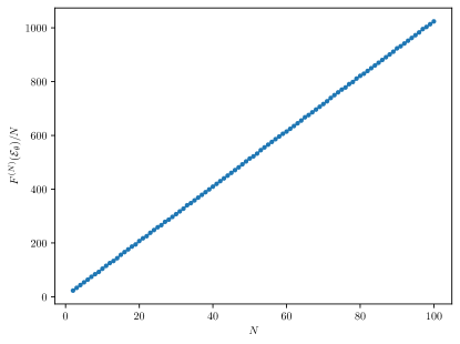
Figure 3: $F^{(N)}(\mathcal{E}_{\theta})/N$ versus the number of channels $N$ for the two-qubit noisy channel estimation, using identical control operations. Allowing different control operations has no significant improvement. The linear plot implies a Heisenberg scaling of the QFI $F^{(N)}(\mathcal{E}_{\theta})$.

III.2 Phase estimation with the bit flip noise

In this section we present a more extensively studied bit flip noise model, and compare our results with some existing works. In the ancilla-free scenario, our result matches a recent finding [43] for achieving the standard quantum limit ($F^{(N)}(\mathcal{E}_{\theta})\propto N$). Assisted by one ancilla, our result outperforms the asymptotically optimal QEC protocol [14, 15, 12].

We would like to estimate $\theta$ from $N$ copies of a quantum channel $\mathcal{E}_{\theta}$ described by the Kraus operators $\{K^{\theta}_{i}=U_{Z}(\theta)K^{(\mathrm{BF})}_{i}\}_{i=1}^{2}$, where $U_{Z}(\theta)=e^{-\mathrm{i}\theta\sigma_{z}/2}$ and

$$K^{(\mathrm{BF})}_{1}=\sqrt{1-p}I,\ K^{(\mathrm{BF})}_{2}=\sqrt{p}\sigma_{x},$$ (20)

for $0\leq p\leq 1$. In numerical experiments, we take $p=0.1$ and the ground truth $\theta=1.0$.

We first apply the optimization algorithm using identical control operations in the ancilla-free scenario, for $N=2$ to $100$ channels. As illustrated in Fig. 4, the growth of $F^{(N)}(\mathcal{E}_{\theta})/N$ slows down as $N$ increases, which implies a standard quantum scaling. We further find out that the control operation $U_{c}$ output by our algorithm is very close to the inverse of the unitary encoding the signal:

$$U_{c}\approx U_{Z}(\theta)^{\dagger}.$$ (21)

Remarkably, this result matches the theoretical finding in a recent work [43, Theorem 5], which states that for this noise model the standard quantum limit can be achieved by nearly reversing the signal encoding unitary in the asymptotic limit. It is worth noting that, however, exactly choosing $U_{c}=U_{Z}(\theta)^{\dagger}$ results in the discontinuity of the QFI, as the matrix rank of the output state $\rho_{\theta}$ changes at this point of $\theta$ [44, 45, 46, 47], and this can also cause the numerical instability of the algorithm. We also apply the first optimization algorithm without the constraint on identical control operations, which, however, does not provide a significant improvement for the metrological performance.

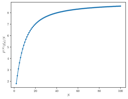
Figure 4: $F^{(N)}(\mathcal{E}_{\theta})/N$ versus the number of channels $N$ for the ancilla-free phase estimation with bit flip noise, using identical control operations. Allowing different control operations has no significant improvement. The plot implies that the QFI $F^{(N)}(\mathcal{E}_{\theta})$ approaches a standard quantum scaling as $N$ grows.

Next, we investigate the performance of the protocol assisted by one ancilla qubit for $N=2$ to $100$ channels. In this case, an asymptotically optimal QEC protocol requiring one ancilla is known [12] and yields a Heisenberg limit $\lim_{N\rightarrow\infty}F^{(\mathrm{N})}(\mathcal{E}_{\theta})/N^{2}=4(1-2p)^{2}$. However, the QEC is not optimal for a finite $N$ [16, 17, 13]. We apply our first algorithm which allows arbitrary control operations in this scenario, and compare the QFI yielded by our tensor network algorithm and that yielded by an optimal QEC protocol, as illustrated in Fig. 5. To make a fairer comparison, we apply $N-1$ QEC recovery operations between $\mathcal{E}_{\theta}$ and do not apply the final recovery operation (which maps the state back to the codespace) at the end. We also make sure that QEC approximately inverts the signal unitary (up to a unitary $e^{\mathrm{-i}\epsilon\sigma_{z}/2}$ with a small $\epsilon=0.01$), otherwise the QFI obtained from QEC significantly decreases due to the discontinuity. We illustrate the metrological performance gap between the QEC protocol and the tensor network algorithm for $N=2$ to $10$ in the inset of Fig. 5. When $N$ gets large (e.g., $N\approx 100$), the relative advantage becomes smaller but still exists. We expect that the relative gap would vanish in the asymptotic limit, as the QEC protocol is asymptotically optimal. Nevertheless, our algorithm provides a higher metrological sensitivity in real-world experiments with finite $N$.

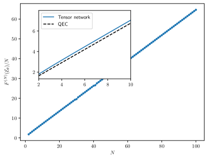
Figure 5: $F^{(N)}(\mathcal{E}_{\theta})/N$ versus the number of channels $N$ for the $1$-ancilla-assisted phase estimation with bit flip noise, using arbitrary control operations. In the inset figure, we show that $F^{(N)}(\mathcal{E}_{\theta})/N$ output by our tensor network algorithm (solid line) is apparently higher than that obtained by an optimal QEC protocol (dashed line) for $N=2$ to $10$. This advantage will become smaller when $N$ is larger (but it still exists for $N=100$), which is expected as the QEC protocol is asymptotically optimal.

IV Conclusions and discussions

We have provided an efficient approach to optimizing control-enhanced metrological strategies by leveraging tensor networks. With its high flexibility for applying arbitrary or identical control operations and assigning the ancilla dimension, we anticipate that this approach is well-suited for real-world experimental demonstration under certain restrictions. This may be particularly suitable for optical experiments, where typically the same control is applied each time with no or small ancilla in an optical loop [18, 19].

Our approach naturally extends its applicability beyond quantum channel estimation. An immediate application is in Hamiltonian parameter estimation with Markovian noise [14, 15, 48], where our framework can be used to identify how the frequency of fast quantum control affects the metrological performance. We can also relax the assumption of estimating $N$ independent channels, but investigate the case where the non-Markovian noise takes effect, induced by the environment which has memory effect [49, 50, 16]. In this case the non-Markovian process can still be expressed as an MPO, with the bond dimension corresponding to the memory [51], so our formalism can also be applicable. Besides, an exciting future work could be developing an efficient approach, possibly based on tensor networks, to optimizing quantum metrology for many-body systems with multi-step control, which handles both spatial complexity and temporal complexity in a unified fashion.

Note added.—After the completion of this work, we learned about an independent work using similar approaches [52]. Note that our approach has a lower computational complexity for computing the derivative of the output state, and is more flexible by allowing for the same quantum control.

Appendix A Proof of Eq. (12)

It is not difficult to verify that Eq. (12) is equivalent to $dE_{\theta}^{\otimes N}/d\theta=\sum_{i=1}^{N}E_{\theta}^{\otimes i-1}\otimes\dot{E}_{\theta}\otimes E_{\theta}^{\otimes N-i}$. Nevertheless, here we provide a diagrammatic method [34] to derive this result in an intuitive way, which has been widely used in compressing sum of local Hamiltonian terms into an MPO.

Without loss of generality, let us consider the case of $N=4$. Then $dE_{\theta}^{\otimes 4}/d\theta=\sum_{i=1}^{4}E_{\theta}^{\otimes i-1}\otimes\dot{E}_{\theta}\otimes E_{\theta}^{\otimes 4-i}$ can be schematically illustrated as a directed graph in Fig. 6. Each term in in the summation $\sum_{i=1}^{4}E_{\theta}^{\otimes i-1}\otimes\dot{E}_{\theta}\otimes E_{\theta}^{\otimes 4-i}$ is represented by a path from the top left vertex to the bottom right vertex.

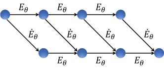
Figure 6: Matrix product diagram for expressing $dE_{\theta}^{\otimes 4}/d\theta$.

Now we see the diagram as a matrix product in this way: each vertex represents a possible value of an index, and $2$ vertices in the same column correspond to $2$ possible values of an index. A directed edge from vertex $i$ to $j$ represents a nonzero matrix element (weight) $M_{ij}$. The diagram can thus be interpreted as a product of $4$ matrices $M_{1},M_{2},M_{3},M_{4}$ (our convention takes a reverse order):

$$(M_{4})_{1\gamma_{3}}(M_{3})_{\gamma_{3}\gamma_{2}}(M_{2})_{\gamma_{2}\gamma_{1}}(M_{1})_{\gamma_{1}1},$$ (22)

where each index $\gamma_{i}$ can take two values $1$ and $2$. According to Fig. 6, we have

$$M_{4}=\begin{pmatrix}E_{\theta}&\dot{E}_{\theta}\end{pmatrix},\ M_{3}=M_{2}=\begin{pmatrix}E_{\theta}&\dot{E}_{\theta}\\ 0&E_{\theta}\end{pmatrix},\ M_{1}=\begin{pmatrix}\dot{E}_{\theta}\\ E_{\theta}\end{pmatrix}.$$ (23)

Noting that each $E_{\theta}$ or $\dot{E}_{\theta}$ is regarded as a tensor with $4$ indices (two $\alpha$ indices and two $\beta$ indices) in Eq. (12), we thus complete the proof for $N=4$. The same argument can be straightforwardly generalized to any $N$.