The study of weak decays of doubly charmed baryons within rescattering mechanism

Abstract

The doubly charmed baryon $\Xi_{cc}^{++}$ has been observed by LHCb through the non-leptonic decay modes of $\Xi_{cc}^{++}\to\Lambda_{c}^{+}K^{-}\pi^{+}\pi^{+}$ and $\Xi_{c}^{+}\pi^{+}$ in 2017. After that, the experimentalists turn their attention to finding other doubly charmed baryons $\Xi_{cc}^{+}$ and $\Omega_{cc}^{+}$. In this work, we investigate the nonleptonic weak decays of doubly charmed baryons ${\cal B}_{cc}\to{\cal B}_{c}P$, where ${\cal B}_{cc}$ denotes the doubly charmed baryons $(\Xi_{cc}^{++},\Xi_{cc}^{+},\Omega_{cc}^{+})$, ${\cal B}_{c}$ represents the singly charmed baryons $({\cal B}_{\bar{3}},{\cal B}_{6})$ and $P$ is the light pseudoscalar. For these non-leptonic decay modes, their short-distance contributions can be accurately estimated in theoretical calculations. However, dealing with the long-distance contributions for final-state-interaction effects is challenging. To address this, we use the rescattering mechanism to calculate the long-distance contributions and first derive the whole hadronic loop contributions for these two-body nonleptonic decays of doubly charmed baryons. Then the decay widths and branching ratios of the 45 nonleptonic decays of doubly charmed baryon are predicted. Among that, the ratio of the branching ratios ${\cal RB}=\frac{{\cal B}(\Xi_{cc}^{++}\to\Xi_{c}^{\prime+}\pi^{+})}{{\cal B}(\Xi_{cc}^{++}\to\Xi_{c}^{+}\pi^{+})}=1.15\pm 0.45$ is consistent with the experimental results within statistical errors.

I Introduction

Doubly heavy baryons, containing two heavy quarks and one light quark, provide a simplified system similar to heavy quarkonia for rigorous non-perturbative theoretical studies of internal structure and strong interaction. High-energy collider experiments are constantly on the lookout for doubly heavy baryons. In 2002, the SELEX collaboration reported the first observation of $\Xi_{cc}^{+}$. However, there has been no confirmation of this discovery by other experiments Ratti:2003ez ; Aubert:2006qw ; Chistov:2006zj ; Aaij:2013voa . It was not until 2017 that the doubly charmed baryon $\Xi_{cc}^{++}$ was discovered via $\Xi_{cc}^{++}\to\Lambda_{c}^{+}K^{-}\pi^{+}\pi^{+}$ and $\Lambda_{c}^{+}\to p\pi^{-}K^{+}$ by the LHCb collaboration Aaij:2017ueg . The existence of doubly charmed baryons $\Xi_{cc}^{++}$ was also verified by this experimental collaboration through the decay channel $\Xi_{cc}^{++}\to\Xi_{c}^{+}\pi^{+}$ Aaij:2018gfl . Before the experiment discovery of $\Xi_{cc}^{++}$, the theoretical study on the weak decays of doubly heavy baryons have been pointed out the most likely discovery of doubly charmed baryons $\Xi_{cc}^{++}$ via the two decay channels $\Xi_{cc}^{++}\to\Lambda_{c}^{+}K^{-}\pi^{+}\pi^{+}$ and $\Xi_{cc}^{++}\to\Xi_{c}^{+}\pi^{+}$ Yu:2017zst . For the experimental reseach of doubly heavy baryons, the pre-theoretical studies of their decays are important.

The heavy to light decay involves large non-perturbative effects. Therefore, theoretical studies cannot be carried out using perturbative QCD methods. Unlike the D meson, there is insufficient experimental data available to extract non-perturbative contributions for the charmed baryon. Theorists have attempted various non-perturbative approaches to study doubly heavy baryon decays, such as light cone sum rules, QCD sum rules, and the light front quark model. These methods have been successful in the study of D mesons and singly heavy baryons. Numerous theoretical studies have been conducted on the weak decay of the doubly heavy baryon. Most theoretical studies focus on semileptonic weak decays, few on two-body nonleptonic decays, the latter being crucial for guiding new particle discoveries, understanding strong interaction dynamics and accurately testing the standard model. The authors in Ref. Yu:2017zst have first studied the non-leptonic decay of doubly charmed baryons, and subsequently give a proposal for the discovery of $\Xi_{cc}^{++}$, using the rescattering mechanism for the final state interaction effects and factorization methods to treat the long and short-distance contributions, respectively. Immediately afterwards, they applied the framework to study the two-body non-leptonic weak decays of a doubly charmed baryon ${\cal B}_{cc}$ decaying into a singly charmed baryon ${\cal B}_{c}$ and a light meson $P(V)$ Han:2021azw ; Jiang:2018oak , and a doubly charmed baryon ${\cal B}_{cc}$ decaying into a light octet baryon ${\cal B}$ and a $D^{(*)}$ meson Li:2020qrh , and a bottom-charm baryon ${\cal B}_{bc}$ decaying into a singly charmed baryon ${\cal B}_{b}$ and a light pseudoscalar meson $P$ Han:2021gkl , theoretically calculated the decay branching ratios for these processes. In the above work, the long-distance contributions were calculated using the cutting rule for the imaginary part of the hadronic triangle diagram. In this work, we will modify the method used in the above works, calculate the total triangle-diagram contribution including the imaginary and real parts, and show the theoretically modified framework in the two-body nonleptonic of double-charmed baryons ${\cal B}_{cc}$ to a single-charmed baryon ${\cal B}_{c}$ and a light pseudoscalar meson $P$.

The factorizable method has been widely used to compute the contribution of the short-distance tree emitted diagram. Therefore, we will not describe the calculation of the factorization method in detail here. Instead, we will focus on illustrating the computation of non-factorizable long-distance contributions using the rescattering mechanism. The doubly charmed baryon decays into one baryon and one meson, which scatter with each other by exchanging one particle into the final states, forming a triangle diagram at the hadron level as shown in Fig. 2. To avoid the double-counting problem, the short-distance and long-distance contributions are separated into the tree emitted process ${\cal B}_{cc}\to P_{1}P_{2}$ and the final states interaction effects. There is an important modify of the framework used in works Yu:2017zst ; Han:2021azw ; Jiang:2018oak ; Li:2020qrh ; Han:2021gkl . In this work, the effective Lagrangian approach is used in the rescattering mechanism to calculate the final states interaction effects. While in the calculations of the final states interaction effects, the non-perturbative parameters such as the cut-off $\Lambda$ in the loop calculation will bring large theoretical uncertainties on the branching ratios. Unlike the case of B meson Ablikim:2002ep ; Cheng:2004ru , there are no enough data to determine the non-perturbative parameters of doubly charmed baryons. Therefore, the main problem in the calculations of long-distance contribution is how to control the theoretical uncertainties. Due to the ratios of the branching fractions are not sensitive to the non-perturbative parameters, we will calculate the ratios to control the uncertainties of the theoretical prediction.

The remainder of this paper is organized as follows. In the section II, we will introduce the theoretical framework of the rescattering mechanism and demonstrate the calculation details with $\Xi_{cc}^{++}\to\Xi_{c}^{+}\pi^{+}$ as an example. In the section III, the input parameters, numerical results of branching fractions and theoretical analysis are presented. In the section IV, we give a brief summary. In the Appendix A, the effective hadron-strong-interaction Lagrangians and corresponding strong coupling constants are collected.

II Theoretical framework

II.1 Effective Hamiltonian and topological diagrams

At the tree level, the non-leptonic weak decays of doubly charmed baryons are induced by the charm quark decays. The effective Hamiltonian can be given by

$$\mathcal{H}_{eff}=\frac{G_{F}}{\sqrt{2}}\sum_{q^{\prime}=d,s}V_{cq^{\prime}}^{\ast}V_{uq}[C_{1}(\mu)O_{1}(\mu)+C_{2}(\mu)O_{2}(\mu)]+h.c..$$ (1)

Here $V_{cq^{\prime}}$ and $V_{uq}$ are the Cabibbo-Kobayashi-Maskawa (CKM) matrix elements. $O_{1}$ and $O_{2}$ are the four-fermion operators,

$$O_{1}=(\bar{u}_{\alpha}q_{\beta})_{V-A}(\bar{q^{\prime}}_{\beta}c_{\alpha})_{V-A},\quad O_{2}=(\bar{u}_{\alpha}q_{\alpha})_{V-A}(\bar{q^{\prime}}_{\beta}c_{\beta})_{V-A},$$ (2)

where the notes $\alpha$ and $\beta$ represent the color indices. And $C_{1,2}(\mu)$ are the relevant Wilson coefficients. After inserting the above effective Hamiltonian, the amplitude of doubly charmed baryons decaying into a singly charmed baryon and a light meson $\mathcal{B}_{cc}\to\mathcal{B}_{c}P$ can be evaluated with the hadronic transition matrix element,

$$\langle\mathcal{B}_{c}P|\mathcal{H}_{eff}|\mathcal{B}_{cc}\rangle=\frac{G_{F}}{\sqrt{2}}V_{cq^{\prime}}^{\ast}V_{uq}\sum_{i=1,2}C_{i}\langle\mathcal{B}_{c}P|O_{i}|\mathcal{B}_{cc}\rangle.$$ (3)

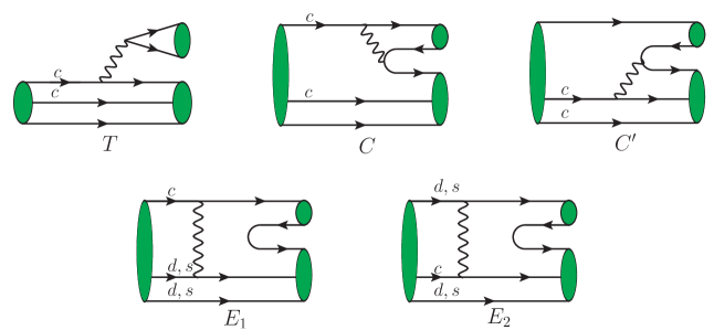
Figure 1: The five tree level topological diagrams for two body non leptonic decays ${\cal B}_{cc}\to{\cal B}_{c}P$ of the doubly charmed baryons ${\cal B}_{cc}=(\Xi_{cc}^{++},\Xi_{cc}^{+},\Omega_{cc}^{+})$.

The weak decays of doubly charmed baryons $\mathcal{B}_{cc}\to\mathcal{B}_{c}P$ involve complicated tree-level contributions. The contributions can be described using several topological diagrams, displayed in Figure 1. Each diagram includes both short-distance and long-distance contributions. Based on their different topologies, the five diagrams can be classified into three types, denoted by $T$, $C(C^{\prime})$ and $E_{1}(E_{2})$. $T$ represents the color-favored external $W$ emission diagram. $C$ and $C^{\prime}$ both designate the color-suppressed internal $W$-emission diagrams. The difference between $C$ and $C^{\prime}$ is whether the two quarks of the final light meson both come from the weak vertex. In the $C$ diagram, the two constituent quarks of the final light meson are all obtained from the weak vertex. Whereas in the $C^{\prime}$ diagram, one constituent quark of the final light meson is obtained from the initial state baryon, and only the antiquark of the final light meson comes from the weak vertex. The $W$-exchange contributions can be classified into two types. In the $E_{1}$ diagram, the light quark, which is produced by the charmed quark decay, is picked up by the final light meson, while in the $E_{2}$ diagram it is picked up by the final charmed baryon.

The calculation of these topological diagrams will be introduced in detail in the following sections. The calculation of $T$ is dominated by the factorizable short-distance contributions, as noted in Ref. Lu:2009cm . The factorization hypothesis can be used to perform this calculation. According to the research Yu:2017zst , the contribution of the $C(C^{\prime})$ diagram can be significantly suppressed at the charm scale due to the color factor $a_{2}(m_{c})=C_{1}(m_{c})+C_{2}(m_{c})/N_{c}$. However, the non-factorizable long-distance contributions may dominate the calculation of the $C(C^{\prime})$ diagram and can have a visible effect on the final amplitude result. At the scale of the charm quark mass, the long-distance contribution dominates over the short-distance contribution in the $E_{1}(E_{2})$ diagram, which is suppressed by at least one order Lu:2009cm .

II.2 Calculation of short-distance amplitudes under the factorization hypothesis

According to the factorization hypothesis, the matrix elements $\langle\mathcal{B}_{c}M|O_{i}|\mathcal{B}_{cc}\rangle$ in Eq. (3) can be factorized into two parts. The first part is parameterized with the decay constant of the emitted meson, while the second part can be evaluated using the heavy-light transition form factors. The short-distance contribution of the $T$ diagram can be expressed as:

$$\langle\mathcal{B}_{c}M|\mathcal{H}_{eff}|\mathcal{B}_{cc}\rangle_{SD}^{T}=\frac{G_{F}}{\sqrt{2}}V_{cq^{\prime}}^{\ast}V_{uq}a_{1}(\mu)\langle M|\bar{u}\gamma^{\mu}(1-\gamma_{5})q|0\rangle\langle\mathcal{B}_{c}|\bar{q}^{\prime}\gamma_{\mu}(1-\gamma_{5})c|\mathcal{B}_{cc}\rangle,$$ (4)

here $a_{1}(\mu)=C_{1}(\mu)+C_{2}(\mu)/3$ is the effective Wilson coefficients. For color suppressed $C$ diagram, its short-distance contribution can be given via its relation to the $T$ diagram after Fierz transformation. And under the charm scale $\mu=m_{c}$, the Wilson coefficients are taken as $C_{1}(\mu)=1.21$ and $C_{2}(\mu)=-0.42$ Li:2012cfa . $M$ represents both pseudoscalar meson($P$) and vector meson($V$). The vector meson also contributes to long-distance dynamics as an intermediate state in the next subsections.

By utilizing the heavy-light transition form factors $f_{1,2,3}$ and $g_{1,2,3}$, the transition matrix elements of ${\cal B}_{cc}\to{\cal B}_{c}$ can be effectively parameterized as,

$$\langle{\cal B}_{c}(p^{\prime},s_{z}^{\prime})|\bar{q}^{\prime}\gamma_{\mu}(1-\gamma_{5})c|{\cal B}_{cc}(p,s_{z})\rangle=\bar{u}(p^{\prime},s_{z}^{\prime})\Big{[}\gamma_{\mu}f_{1}(q^{2})+i\sigma_{\mu\nu}\frac{q^{\nu}}{M_{\mathcal{B}_{cc}}}f_{2}(q^{2})+\frac{q^{\mu}}{M_{\mathcal{B}_{cc}}}f_{3}(q^{2})\Big{]}u(p,s_{z})$$

$$\quad\quad\quad\quad\quad\quad\quad\quad\quad\quad\quad\quad-\bar{u}(p^{\prime},s_{z}^{\prime})\Big{[}\gamma_{\mu}g_{1}(q^{2})+i\sigma_{\mu\nu}\frac{q^{\nu}}{M_{\mathcal{B}_{cc}}}g_{2}(q^{2})+\frac{q^{\mu}}{M_{\mathcal{B}_{cc}}}g_{3}(q^{2})\Big{]}\gamma_{5}u(p,s_{z}).$$ (5)

Here $q=p-p^{\prime}$, $M_{\mathcal{B}_{cc}}$ is the mass of doubly charmed baryons.

The first matrix element in Eq. (4) are defined using the decay constants of the emitted mesons $P$ and $V$, denoted by $f_{P}$ and $f_{V}$, respectively.

$$\langle P(p)|\bar{u}\gamma^{\mu}(1-\gamma_{5})q|0\rangle =-if_{P}p^{\mu},$$ (6)

$$\langle V(p)|\bar{u}\gamma^{\mu}(1-\gamma_{5})q|0\rangle =m_{V}f_{V}\epsilon^{\ast\mu},$$ (7)

where $\epsilon^{\mu}$ represents the polarization vector of the vector meson.

Substituting Eqs. (5-7) into Eq. (4), the short-distance amplitudes of the weak decays ${\cal B}_{cc}\to{\cal B}_{c}P$ and $\mathcal{B}_{c}V$ can be written as,

$$\mathcal{A}({\cal B}_{cc}\to{\cal B}_{c}P) =i\bar{u}_{\mathcal{B}_{c}}(A+B\gamma_{5})u_{\mathcal{B}_{cc}},$$ (8)

$$\mathcal{A}({\cal B}_{cc}\to{\cal B}_{c}V) =\epsilon^{\ast\mu}\bar{u}_{\mathcal{B}_{c}}\left[A_{1}\gamma_{\mu}\gamma_{5}+A_{2}\frac{p_{\mu}(\mathcal{B}_{c})}{M_{\mathcal{B}_{cc}}}\gamma_{5}+B_{1}\gamma_{\mu}+B_{2}\frac{p_{\mu}(\mathcal{B}_{c})}{M_{\mathcal{B}_{cc}}}\right]u_{\mathcal{B}_{cc}}.$$ (9)

Here the parameters $A,B$ and $A_{1,2},B_{1,2}$, describing the information of strong interaction, are expressed as within the factorization approach.

$$A =\lambda f_{P}(M_{\mathcal{B}_{cc}}-M_{\mathcal{B}_{c}})f_{1}(m^{2}),\hskip 85.35826ptB=\lambda f_{P}(M_{\mathcal{B}_{cc}}+M_{\mathcal{B}_{c}})g_{1}(m^{2}),$$ (10)

$$A_{1} =-\lambda f_{V}m\left(g_{1}(m^{2})+g_{2}(m^{2})\frac{M_{\mathcal{B}_{cc}}-M_{\mathcal{B}_{c}}}{M_{\mathcal{B}_{cc}}}\right),\ \ \ \ A_{2}=-2\lambda f_{V}mg_{2}(m^{2}),$$ (11)

$$B_{1} =\lambda f_{V}m\left(f_{1}(m^{2})-f_{2}(m^{2})\frac{M_{\mathcal{B}_{cc}}+M_{\mathcal{B}_{c}}}{M_{\mathcal{B}_{cc}}}\right),\ \ \ \ \ \ \ \ B_{2}=2\lambda f_{V}mf_{2}(m^{2}),$$ (12)

where the parameter $\lambda$ is $\frac{G_{F}}{\sqrt{2}}V_{CKM}a_{1,2}(\mu)$, and $m$ is the mass of pseudoscalar or vector meson. We exclude $f_{3}$ and $g_{3}$ terms in Eq. (5) due to $m^{2}/M_{\mathcal{B}_{cc}}^{2}$ suppression.

II.3 Calculation of long-distance contributions using the rescattering mechanism

The long-distance contributions are large and very difficult to evaluate. In this work, we employ the rescattering mechanism to perform the calculation of the long-distance contributions, as done in Ref. Yu:2017zst . Via rescattering of two intermediate particles, the rescattering mechanism can be constructed as shown in Fig. 2. This mechanism involves the final state interaction effects which can be calculated using the hadronic strong-interaction effective Lagrangian. In the following, we take the decay $\Xi_{cc}^{++}\to\Xi_{c}^{+}\pi^{+}$ as an example to explain the detail of our calculation. This decay can proceed as $\Xi_{cc}^{++}\to\Xi_{c}^{+}(\Xi_{c}^{\prime+})\pi^{+}(\rho^{+})\to\Xi_{c}^{+}\pi^{+}$, as shown in Fig. 3. At the quark level, the first weak vertex of the triangle diagram is induced by $c\to sud$, which indicates that it is a CKM-favored decay. At the hadron level, the intermediate particles, anti-triplet(sextet)singly charmed baryons $\Xi_{c}^{+}(\Xi_{c}^{\prime+})$ and light pseudoscalar(vector)mesons $\pi^{+}(\rho^{+})$ originates from $T$ diagram. Using the factorization hypothesis, the weak vertex only involving short-distance contributions can be evaluated. The upcoming scattering process can occur via either an $s$ channel or a $t/u$ channel. The diagram of $s$ channel would make a sizable contribution when the mass of the exchanged particle is the sequel to the ones of the mother particle $\Xi_{cc}^{++}$. While the heaviest discovered singly charmed baryon is approximately $500$MeV lighter than $m_{\Xi_{cc}^{+}}$. So the contribution of the $s$-channel diagram is supposed to be highly suppressed by the off-shell effect and can be safely neglected. As a result, we only consider the contribution of the $t/u$-channel triangle diagram, as depicted in Fig. 3. Then the other two strong interaction vertexes, as shown in Fig. 3, can be evaluated by the hadronic strong interaction Lagrangians, which have been listed in the Appendix A.

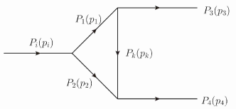
Figure 2: The diagram description of the rescattering mechanism at the hadron level.

In Figure 2, the particles labeled $P_{i,3,4}$ represent initial and final states, while the particles labeled $P_{1,2,k}$ represent intermediate states. Their momenta are $p_{i,3,4}$, and $p_{1,2,k}$, respectively. We use the symbol $\mathcal{M}(P_{1},P_{2},P_{k})$ to represent a triangle amplitude in this work. There are various ways to compute the triangle amplitude Li:2002pj ; Ablikim:2002ep ; Li:1996cj ; Dai:1999cs ; Locher:1993cc ; Cheng:2004ru ; Lu:2005mx . The main point of distinction between them is their approach towards the integration of hadronic loops. In the work Han:2021azw , the authors adopting the optical theorem and Cutkosky cutting rule as in Ref. Cheng:2004ru , only calculate the absorptive (imaginary) part of these diagrams. In this work, the whole amplitudes, not only the absorptive part of these diagrams but also the dispersive ones, will be calculated.

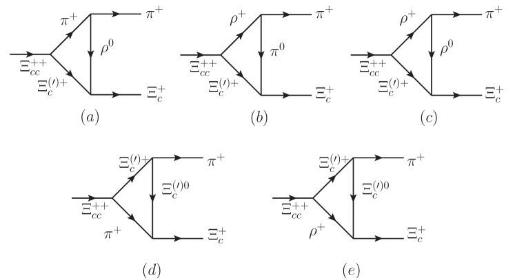
Figure 3: The long-distance rescattering contributions to $\Xi_{cc}^{++}\to\Xi_{c}^{+}\pi^{+}$ manifested at hadron level.

To clarify, we want to determine the amplitude of the decay mode for $\Xi_{cc}^{++}\to\Xi_{c}^{+}\pi^{+}$. The Fig. 3(a) shows a triangle diagram with intermediate states $\{\pi^{+},\Xi_{c}^{+}(\Xi_{c}^{\prime+}),\rho^{0}\}$, involving a weak vertex $\Xi_{cc}^{++}\to\Xi_{c}^{+}(\Xi_{c}^{\prime+})\pi^{+}$, as well as a rescattering amplitude of $\Xi_{c}^{+}(\Xi_{c}^{\prime+})\pi^{+}\to\Xi_{c}^{+}\pi^{+}$. The factorization approach in Eq. (8) can calculate the weak vertex, while the rescattering amplitude is computed using the hadronic strong Lagrangian. The entire amplitude shown in Figure 3(a) can be expressed as:

$${\cal{M}}[\pi^{+},\Xi_{c}^{(\prime)+},\rho^{0}] = \int\frac{d^{4}p_{1}}{(2\pi)^{4}}\bar{u}(p_{4},s_{4})(f_{1\Xi_{c}^{(\prime)+}\Xi_{c}^{+}\rho^{0}}\gamma_{\nu}-\frac{if_{2\Xi_{c}^{(\prime)+}\Xi_{c}^{+}\rho^{0}}}{m_{2}+m_{4}}\sigma_{\mu\nu}p_{k}^{\mu})(\not{p}_{2}+m_{2})$$ (13)

$$\times i(A+B\gamma_{5})u(p_{i},s_{i})(-ig_{\rho\pi\pi})(-g^{\alpha\nu}+\frac{p_{k}^{\alpha}p_{k}^{\nu}}{m_{k}^{2}})(p_{1}+p_{3})_{\alpha}{\cal{PF}},$$

where the note ${\cal{PF}}$ represents the multiply of the propagators and form factors,

$${\cal{PF}} = \frac{i}{p_{1}^{2}-m_{1}^{2}+i\epsilon}\frac{i}{p_{2}^{2}-m_{2}^{2}+i\epsilon}\frac{i}{p_{k}^{2}-m_{k}^{2}+i\epsilon}\frac{\Lambda_{k}^{2}-m_{k}^{2}}{\Lambda_{k}^{2}-p_{k}^{2}}.$$ (14)

In the given equation, strong coupling constants, $g_{\rho\pi\pi}$, $f_{1\Xi_{(\prime)c}^{+}\Xi_{c}^{+}\rho^{0}}$, and $f_{2\Xi_{c}^{(\prime)+}\Xi_{c}^{+}\rho^{0}}$ are calculated on-shell. The reliability of the strong coupling constants is compromised due to the exchange states $\rho^{0}$ being generally off-shell. The form factor of the exchange particle $F(p_{j},m_{j})$ are introduced to account for off-shell effects and self-consistency of the theoretical framework Cheng:2004ru ,

$$F(p_{k},m_{k})=\left(\frac{\Lambda_{k}^{2}-m_{k}^{2}}{\Lambda_{k}^{2}-p_{k}^{2}}\right)^{n}.$$ (15)

The cutoff $\Lambda_{j}$ can be given as

$$\Lambda_{k}=m_{k}+\eta\Lambda_{{\rm QCD}}.$$ (16)

with $\Lambda_{{\rm QCD}}=330\text{MeV}$ for the charm quark decays. The phenomenological parameter $\eta$ depends on particles at the strong vertex and is determined by experimental data. In this work, multiple strong vertices require extensive experimental data for individual parameter calculation. In the next section, we will examine how varying the parameter $\eta$ from 1 to 2 affects the results. Eq. (15) typically exhibits monopole or dipole behavior, with the exponential factor n taking on values of 1 or 2. The branching ratios for $B$ meson decays in Ref. Cheng:2004ru are similar for both choices, so we select $n=1$ for convenience.

Similarly, the amplitude of the remaining diagrams in Fig. 3 can be derived as follows,

$${\cal{M}}[\rho^{+},\Xi_{c}^{(\prime)+};\pi^{0}] = \int\frac{d^{4}p_{1}}{(2\pi)^{4}}ig_{\pi^{0}\Xi_{c}^{(\prime)+}\Xi_{c}^{+}}\bar{u}(p_{4},s_{4})i\gamma_{5}({\not{p}}_{2}+m_{2})$$ (17)

$$\times i(-g^{\rho\alpha}+\frac{p_{1}^{\rho}p_{1}^{\alpha}}{m_{1}^{2}})(A_{1}\gamma_{\rho}\gamma_{5}+A_{2}\frac{p_{2\rho}}{m_{i}}\gamma_{5}+B_{1}\gamma_{\rho}+B_{2}\frac{p_{2\rho}}{m_{i}})u(p_{i},s_{i})$$

$$\times ig_{\rho^{+}\pi^{0}\pi^{+}}(p_{3}-p_{k})_{\alpha}{\cal PF},$$

$${\cal{M}}[\rho^{+},\Xi_{c}^{(\prime)+};\rho^{0}] = \int\frac{d^{4}p_{1}}{(2\pi)^{4}}\bar{u}(p_{4},s_{4})(f_{1\Xi_{c}^{(\prime)+}\Xi_{c}^{+}\rho^{0}}\gamma^{\nu}-\frac{if_{2\Xi_{c}^{(\prime)+}\Xi_{c}^{+}\rho^{0}}}{m_{2}+m_{4}}\sigma^{\mu\nu}p_{k\mu})$$ (18)

$$\times(\not{p}_{2}+m_{2})i(A_{1}\gamma^{\rho}\gamma_{5}+A_{2}\frac{p_{2}^{\rho}}{m_{i}}\gamma_{5}+B_{1}\gamma^{\rho}+B_{2}\frac{p_{2}^{\rho}}{m_{i}})u(p_{i},s_{i})$$

$$\times(-i\frac{g_{\rho\rho\pi}}{f_{\pi}})\epsilon^{\alpha\beta\delta\sigma}p_{k\alpha}p_{1\delta}(-g_{\rho\sigma}+\frac{p_{1\rho}p_{1\sigma}}{m_{1}^{2}})(-g_{\nu\beta}+\frac{p_{k\nu}p_{k\beta}}{m_{k}^{2}}){\cal{PF}},$$

$${\cal{M}}[\Xi_{c}^{(\prime)+},\pi^{+};{\Xi}_{c}^{(\prime)0}] = \int\frac{d^{4}p_{1}}{(2\pi)^{4}}ig_{\pi^{+}{\Xi}_{c}^{(\prime)0}\Xi_{c}^{+}}\bar{u}(p_{4},s_{4})i\gamma_{5}(\not{p}_{k}+m_{k})ig_{\pi^{+}{\Xi}_{c}^{(\prime)0}\Xi_{c}^{(\prime)+}}i\gamma_{5}(\not{p}_{1}+m_{1})$$ (19)

$$\times i(A+B\gamma_{5})u(p_{i},s_{i}){\cal PF},$$

$${\cal{M}}[\Xi_{c}^{(\prime)+},\rho^{+};{\Xi}_{c}^{(\prime)0}] = \int\frac{d^{4}p_{1}}{(2\pi)^{4}}\bar{u}(p_{4},s_{4})(f_{1\rho^{+}{\Xi}_{c}^{(\prime)0}\Xi_{c}^{+}}\gamma_{\nu}-\frac{if_{2\rho^{+}{\Xi}_{c}^{(\prime)0}\Xi_{c}^{+}}}{m_{k}+m_{4}}\sigma_{\mu\nu}p_{2}^{\mu})$$ (20)

$$\times(\not{p}_{k}+m_{k})ig_{\pi^{+}{\Xi}_{c}^{(\prime)0}\Xi_{c}^{(\prime)+}}i\gamma_{5}(\not{p}_{1}+m_{1})(-g_{\nu\rho}+\frac{p_{2\nu}p_{2\rho}}{m_{2}^{2}})$$

$$\times i(A_{1}\gamma_{\rho}\gamma_{5}+A_{2}\frac{p_{1\rho}}{m_{i}}\gamma_{5}+B_{1}\gamma_{\rho}+B_{2}\frac{p_{1\rho}}{m_{i}})u(p_{i},s_{i}){\cal PF}.$$

After gathering all the fragments, the amplitude of decay $\Xi_{cc}^{++}\to\Xi_{c}^{+}\pi^{+}$ can be expressed as:

$$\mathcal{A}(\Xi_{cc}^{++}\to\Xi_{c}^{+}\pi^{+}) =T_{SD}(\Xi_{cc}^{++}\to\Xi_{c}^{+}\pi^{+})+\mathcal{M}[\pi^{+},\Xi_{c}^{(\prime)+};\rho^{0}]+\mathcal{M}[\rho^{+},\Xi_{c}^{(\prime)+};\pi^{0}]$$

$$+\mathcal{M}[\rho^{+},\Xi_{c}^{(\prime)+};\rho^{0}]+\mathcal{M}[\Xi_{c}^{(\prime)+},\pi^{+};\Xi_{c}^{(\prime)0}]+\mathcal{M}[\Xi_{c}^{(\prime)+},\rho^{+};\Xi_{c}^{(\prime)0}],$$ (21)

where $T_{SD}$ labels its short-distance contributions. The amplitudes for all the other channels can be derived in the same way, and can be found in Appendix.

At the rest frame of doubly charmed baryons $\mathcal{B}_{cc}$, the calculation of the decay width of $\mathcal{B}_{cc}\to\mathcal{B}_{c}P$ can be done.

$$\Gamma(\mathcal{B}_{cc}\to\mathcal{B}_{c}P)=\frac{\sqrt{[m_{\mathcal{B}_{cc}}^{2}-(m_{\mathcal{B}_{c}}+m_{P})^{2}][m_{\mathcal{B}_{cc}}^{2}-(m_{\mathcal{B}_{c}}-m_{P})^{2}]}}{16\pi m_{\mathcal{B}_{cc}}^{2}}\frac{1}{2}\sum_{s_{i},s_{4}}\Big{|}\mathcal{A}(\mathcal{B}_{cc}\to\mathcal{B}_{c}P)\Big{|}^{2}.$$ (22)

where $s_{i}$ and $s_{4}$ denote the spin of initial and final states.

III Numerical results and discussions

Table 1: Decay constants (in units of MeV) of the light pseudoscalar and vector mesons used in this work Workman:2022ynf ; Choi:2015ywa ; Feldmann:1998vh .

$f_{\pi}$	$f_{\eta_{1}}$	$f_{\rho}$	$f_{\omega}$	$f_{\eta_{8}}$	$f_{\phi}$	$f_{K}$	$f_{K^{*}}$
$130$	$152$	$216$	$195$	$163$	$233$	$156$	$217$

Calculation of decay widths requires inputs such as initial and final state masses, decay constants of pseudoscalar and vector mesons, strong couplings, and transition form factors, as shown in Eqs. (13-22). Besides, calculating the branching fractions requires knowing the lifetimes of the doubly charmed baryons, as $\mathcal{BR}_{i}=\Gamma_{i}\cdot\tau$. The LHCb collaboration has successfully measured the mass and lifetime of $\Xi_{cc}^{++}$: $m_{\Xi_{cc}^{++}}=3.621$ MeVAaij:2017ueg ; Aaij:2018gfl , $\tau_{\Xi_{cc}^{++}}=256$ fsAaij:2018wzf . After these measurements, many theoretical works have studied the masses and lifetimes of doubly charmed baryons Workman:2022ynf ; Chen:2016spr ; Yu:2018com ; Yu:2019lxw ; Cheng:2018mwu ; Berezhnoy:2018bde . The measurement of $\Xi_{cc}^{++}$ would benefit theoretical predictions on the other doubly charmed baryons. The results from Refs. Yu:2018com ; Berezhnoy:2018bde are adopted in this work, $m_{\Xi_{cc}^{+}}=3.621$ MeV, $m_{\Omega_{cc}^{+}}=3.738$ MeV,$\tau_{\Xi_{cc}^{+}}=44$ fs and $\tau_{\Omega_{cc}^{+}}=206$ fs. The masses of the final states including singly heavy baryons, light pseudoscalar and vector mesons, can be easily found in Particle Data Group Workman:2022ynf . The decay constants of pseudoscalar and vector mesons are obtained from the literature Workman:2022ynf ; Choi:2015ywa ; Feldmann:1998vh , and summarised in Tab. 1. The form factors of the transition $\mathcal{B}_{cc}\to\mathcal{B}_{c}$ have been calculated in many works Wang:2017mqp . In this work, we utilize the theoretical results of form factors within the light-front quark model, which have been successfully used to predict the discovery channel of $\Xi_{cc}^{++}$ in Ref. Yu:2017zst . Besides, the strong coupling constants of the various hadrons are also required, most of them are taken from theoretical works Aliev:2010yx ; Yan:1992gz ; Casalbuoni:1996pg ; Meissner:1987ge ; Li:2012bt ; Aliev:2010nh . Some strong couplings are not available in the literature, we calculate them under the flavor $SU(3)$ symmetry.

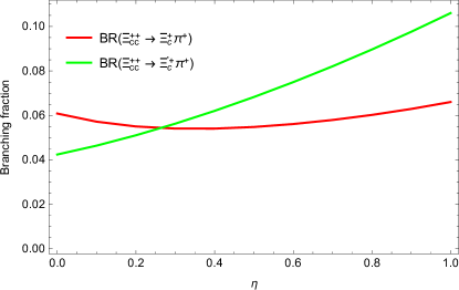
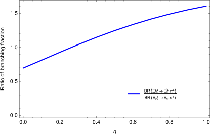
Figure 4: (a): The theoretical predictions for the branching fractions of $\Xi_{cc}^{++}\to\Xi_{c}^{+}\pi^{+}$ and $\Xi_{cc}^{++}\to\Xi_{c}^{\prime+}\pi^{+}$ in logarithmic coordinates; (b): Ratio of branching fractions with $\eta$ varying from $0$ to $1.0$

In order to describe the off-shell effect of the exchange particles, one form factor is introduced as given in Eq. (15). In this form factor, the parameter $\eta$ is usually calculated from the experimental data as in Cheng:2004ru . In the case of doubly charmed baryon decays, the lack of data for the calculation of $\eta$ will lead to large uncertainties in the theoretical predictions of the branching fractions. Fig. 4(a) shows branching fractions for $\Xi_{cc}^{++}\to\Xi_{c}^{+}\pi^{+}$ and $\Xi_{cc}^{++}\to\Xi_{c}^{\prime+}\pi^{+}$ as a function of $\eta$. The branching fractions are highly dependent on the value of the parameter $\eta$. With $\eta$ varying between $0$ and $1$, the branching fractions could change by almost an order of magnitude. This is a well-known issue with final state interaction effects, which have large theoretical uncertainties. While as depicted in Fig.4(b), the ratio of the two branching fractions is

$${\cal RB}=\frac{{\cal B}(\Xi_{cc}^{++}\to\Xi_{c}^{\prime+}\pi^{+})}{{\cal B}(\Xi_{cc}^{++}\to\Xi_{c}^{+}\pi^{+})}=1.15\pm 0.45,$$ (23)

which is consistence with the experiment data $1.41\pm 0.17\pm 0.10$ within statistical errors. As a result, the uncertainty of the ratio is $39\%$ from the parameter $\eta$. In this work, we present the numerical predictions of branching fractions with $\eta=0.1,0.5,1.0$, to show the absolute uncertainty of each mode. In order to get a more reliable result, we can take a ratio between any two processes.

Table 2: Branching ratios for the short-distance dynamics dominated modes. The “CF”, “SCS” and “DCS” represent CKM favored, singly CKM suppressed and doubly CKM suppressed processes, respectively.

channels	Topology	${\cal BR}_{T_{SD}}$	${\cal B}_{\eta=0.1}$	${\cal B}_{\eta=0.5}$	${\cal B}_{\eta=1}$	CKM
$\Xi_{cc}^{++}\to\Xi_{c}^{+}\pi^{+}$	$\lambda_{sd}(T+C^{\prime})$	$6.08\times 10^{-2}$	$5.72\times 10^{-2}$	$5.48\times 10^{-2}$	$6.60\times 10^{-2}$	CF
$\Xi_{cc}^{++}\to\Xi_{c}^{\prime+}\pi^{+}$	$\frac{1}{\sqrt{2}}\lambda_{sd}\big{(}\tilde{T}+\tilde{C}^{\prime}\big{)}$	$4.24\times 10^{-2}$	$4.64\times 10^{-2}$	$6.83\times 10^{-2}$	$1.06\times 10^{-1}$	CF
$\Xi_{cc}^{++}\to\Sigma_{c}^{+}\pi^{+}$	$\frac{1}{\sqrt{2}}\lambda_{d}\big{(}\tilde{T}+\tilde{C}^{\prime}\big{)}$	$2.26\times 10^{-3}$	$2.73\times 10^{-3}$	$4.77\times 10^{-3}$	$7.96\times 10^{-3}$	SCS
$\Xi_{cc}^{++}\to\Lambda_{c}^{+}\pi^{+}$	$\lambda_{d}(T+C^{\prime})$	$3.50\times 10^{-3}$	$3.60\times 10^{-3}$	$4.09\times 10^{-3}$	$4.71\times 10^{-3}$	SCS
$\Xi_{cc}^{++}\to\Xi_{c}^{\prime+}K^{+}$	$\frac{1}{\sqrt{2}}\lambda_{s}\big{(}\tilde{T}+\tilde{C}^{\prime}\big{)}$	$2.78\times 10^{-3}$	$3.54\times 10^{-3}$	$8.70\times 10^{-3}$	$1.92\times 10^{-2}$	SCS
$\Xi_{cc}^{++}\to\Xi_{c}^{+}K{+}$	$\lambda_{s}(T+C^{\prime})$	$4.90\times 10^{-3}$	$5.56\times 10^{-3}$	$1.21\times 10^{-2}$	$2.54\times 10^{-2}$	SCS
$\Xi_{cc}^{++}\to\Lambda_{c}^{+}K^{+}$	$\lambda_{ds}(T+C^{\prime})$	$2.96\times 10^{-4}$	$2.82\times 10^{-4}$	$2.51\times 10^{-4}$	$2.47\times 10^{-4}$	DCS
$\Xi_{cc}^{++}\to\Sigma_{c}^{+}K^{+}$	$\frac{1}{\sqrt{2}}\lambda_{ds}\big{(}\tilde{T}+\tilde{C}^{\prime}\big{)}$	$1.60\times 10^{-4}$	$1.78\times 10^{-4}$	$2.63\times 10^{-4}$	$3.87\times 10^{-4}$	DCS
$\Xi_{cc}^{+}\to\Xi_{c}^{0}\pi^{+}$	$\lambda_{sd}(T-E_{2})$	$1.04\times 10^{-2}$	$1.03\times 10^{-2}$	$1.09\times 10^{-2}$	$1.36\times 10^{-2}$	CF
$\Xi_{cc}^{+}\to\Xi_{c}^{\prime 0}\pi^{+}$	$\frac{1}{\sqrt{2}}\lambda_{sd}\big{(}\tilde{T}+\tilde{E}_{2}\big{)}$	$7.27\times 10^{-3}$	$6.95\times 10^{-3}$	$5.90\times 10^{-3}$	$4.96\times 10^{-3}$	CF
$\Xi_{cc}^{+}\to\Sigma_{c}^{0}\pi^{+}$	$\lambda_{d}(\tilde{T}+\tilde{E}_{2})$	$7.77\times 10^{-4}$	$7.93\times 10^{-4}$	$8.25\times 10^{-4}$	$8.08\times 10^{-4}$	SCS
$\Xi_{cc}^{+}\to\Xi_{c}^{\prime 0}K^{+}$	$\frac{1}{\sqrt{2}}\big{(}\lambda_{s}\tilde{T}+\lambda_{d}\tilde{E}_{2}\big{)}$	$4.77\times 10^{-4}$	$5.61\times 10^{-4}$	$1.10\times 10^{-3}$	$2.08\times 10^{-3}$	SCS
$\Xi_{cc}^{+}\to\Xi_{c}^{0}K{+}$	$\lambda_{s}T+\lambda_{d}E_{2}$	$8.37\times 10^{-4}$	$8.82\times 10^{-4}$	$1.16\times 10^{-3}$	$1.64\times 10^{-3}$	SCS
$\Xi_{cc}^{+}\to\Sigma_{c}^{0}K^{+}$	$\lambda_{ds}\tilde{T}$	$1.01\times 10^{-3}$	$1.01\times 10^{-3}$	$1.01\times 10^{-3}$	$1.01\times 10^{-3}$	DCS
$\Omega_{cc}^{+}\to\Omega_{c}^{0}\pi^{+}$	$\lambda_{sd}\tilde{T}$	$6.82\times 10^{-2}$	$6.82\times 10^{-2}$	$6.82\times 10^{-2}$	$6.82\times 10^{-2}$	CF
$\Omega_{cc}^{+}\to\Xi_{c}^{0}\pi^{+}$	$-\lambda_{d}T-\lambda_{s}E_{2}$	$2.49\times 10^{-3}$	$2.61\times 10^{-3}$	$3.19\times 10^{-3}$	$3.99\times 10^{-3}$	SCS
$\Omega_{cc}^{+}\to\Xi_{c}^{\prime 0}\pi^{+}$	$\frac{1}{\sqrt{2}}\big{(}\lambda_{d}\tilde{T}+\lambda_{s}\tilde{E}_{2}\big{)}$	$1.78\times 10^{-3}$	$2.14\times 10^{-3}$	$3.82\times 10^{-3}$	$6.16\times 10^{-3}$	SCS
$\Omega_{cc}^{+}\to\Omega_{c}^{0}K^{+}$	$\lambda_{s}\big{(}\tilde{T}+\tilde{E}_{2}\big{)}$	$4.51\times 10^{-3}$	$5.35\times 10^{-3}$	$1.05\times 10^{-2}$	$1.95\times 10^{-2}$	SCS
$\Omega_{cc}^{+}\to\Xi_{c}^{0}K^{+}$	$\lambda_{ds}(-T+E_{2})$	$2.10\times 10^{-4}$	$2.10\times 10^{-4}$	$2.06\times 10^{-4}$	$1.97\times 10^{-4}$	DCS
$\Omega_{cc}^{+}\to\Xi_{c}^{\prime 0}K^{+}$	$\frac{1}{\sqrt{2}}\lambda_{ds}\big{(}\tilde{T}+\tilde{E}_{2}\big{)}$	$1.26\times 10^{-4}$	$1.32\times 10^{-4}$	$1.60\times 10^{-4}$	$1.97\times 10^{-4}$	DCS

Table 3: Branching ratios for the long-distance dominated Cabibbo-favored ($\lambda_{sd}$) modes. For the channels involving internal W-emission contributions, the short-distance factorizable contributions are also listed in the fourth column for comparison

channels	Topology	${\cal BR}_{T_{SD}}$	${\cal B}_{\eta=0.1}$	${\cal B}_{\eta=0.5}$	${\cal B}_{\eta=1}$
$\Xi_{cc}^{++}\to\Sigma_{c}^{++}\bar{K}^{0}$	$\tilde{C}$	$1.54\times 10^{-5}$	$2.32\times 10^{-3}$	$4.38\times 10^{-2}$	$1.37\times 10^{-1}$
$\Xi_{cc}^{+}\to\Omega_{c}^{0}K^{+}$	$\tilde{E}_{2}$		$2.09\times 10^{-5}$	$4.95\times 10^{-4}$	$1.83\times 10^{-3}$
$\Xi_{cc}^{+}\to\Sigma_{c}^{+}\bar{K}^{0}$	$\frac{1}{\sqrt{2}}\big{(}\tilde{C}+\tilde{E}_{1}\big{)}$	$1.31\times 10^{-6}$	$1.69\times 10^{-4}$	$3.12\times 10^{-3}$	$9.59\times 10^{-3}$
$\Xi_{cc}^{+}\to\Lambda_{c}^{+}\bar{K}^{0}$	$-C+E_{1}$	$2.62\times 10^{-6}$	$6.52\times 10^{-4}$	$1.24\times 10^{-2}$	$3.82\times 10^{-2}$
$\Xi_{cc}^{+}\to\Sigma_{c}^{++}K^{-}$	$\tilde{E}_{1}$		$7.29\times 10^{-5}$	$1.53\times 10^{-3}$	$4.99\times 10^{-3}$
$\Xi_{cc}^{+}\to\Xi_{c}^{\prime+}\pi^{0}$	$\frac{1}{2}(-\tilde{C}^{\prime}+\tilde{E}_{2})$		$5.66\times 10^{-6}$	$1.41\times 10^{-4}$	$5.46\times 10^{-4}$
$\Xi_{cc}^{+}\to\Xi_{c}^{\prime+}\eta_{1}$	$\frac{1}{\sqrt{6}}(\tilde{C}^{\prime}+\tilde{E}_{1}+\tilde{E}_{2})$		$8.98\times 10^{-7}$	$1.77\times 10^{-5}$	$5.51\times 10^{-5}$
$\Xi_{cc}^{+}\to\Xi_{c}^{\prime+}\eta_{8}$	$\frac{1}{2\sqrt{3}}(\tilde{C}^{\prime}-2\tilde{E}_{1}+\tilde{E}_{2})$		$9.62\times 10^{-8}$	$2.04\times 10^{-6}$	$6.64\times 10^{-6}$
$\Xi_{cc}^{+}\to\Xi_{c}^{+}\pi^{0}$	$-\frac{1}{\sqrt{2}}(C^{\prime}+E_{2})$		$3.82\times 10^{-5}$	$6.46\times 10^{-4}$	$1.62\times 10^{-3}$
$\Xi_{cc}^{+}\to\Xi_{c}^{+}\eta_{1}$	$\frac{1}{\sqrt{3}}(C^{\prime}+E_{1}-E_{2})$		$7.81\times 10^{-7}$	$1.54\times 10^{-5}$	$4.72\times 10^{-5}$
$\Xi_{cc}^{+}\to\Xi_{c}^{+}\eta_{8}$	$\frac{1}{\sqrt{6}}(C^{\prime}-2E_{1}-E_{2})$		$6.73\times 10^{-6}$	$1.62\times 10^{-4}$	$6.86\times 10^{-4}$
$\Omega_{cc}^{+}\to\Xi_{c}^{\prime+}\bar{K}^{0}$	$\frac{1}{\sqrt{2}}(\tilde{C}+\tilde{C}^{\prime})$	$8.61\times 10^{-6}$	$1.39\times 10^{-3}$	$3.14\times 10^{-2}$	$1.08\times 10^{-1}$
$\Omega_{cc}^{+}\to\Xi_{c}^{+}\bar{K}^{0}$	$-C+C^{\prime}$	$1.72\times 10^{-5}$	$4.14\times 10^{-3}$	$9.59\times 10^{-2}$	$3.59\times 10^{-1}$

Table 4: Same as Table.3 but for the long-distance dominated singly Cabibbo-suppressed modes.

channels	Topology	${\cal BR}_{T_{SD}}$	${\cal B}_{\eta=0.1}$	${\cal B}_{\eta=0.5}$	${\cal B}_{\eta=1}$
$\Xi_{cc}^{++}\to\Sigma_{c}^{++}\pi^{0}$	$-\frac{1}{\sqrt{2}}\tilde{C}$	$4.41\times 10^{-7}$	$6.55\times 10^{-5}$	$1.65\times 10^{-3}$	$5.76\times 10^{-3}$
$\Xi_{cc}^{++}\to\Sigma_{c}^{++}\eta_{1}$	$\frac{1}{\sqrt{3}}(\lambda_{d}+\lambda_{s})\tilde{C}$	$4.12\times 10^{-7}$	$7.97\times 10^{-6}$	$1.22\times 10^{-4}$	$3.57\times 10^{-4}$
$\Xi_{cc}^{++}\to\Sigma_{c}^{++}\eta_{8}$	$\frac{1}{\sqrt{6}}(\lambda_{d}-2\lambda_{s})\tilde{C}$	$2.06\times 10^{-7}$	$1.04\times 10^{-5}$	$2.41\times 10^{-4}$	$7.72\times 10^{-4}$
$\Xi_{cc}^{+}\to\Sigma_{c}^{+}\pi^{0}$	$\frac{1}{2}\lambda_{d}\big{(}-\tilde{C}-\tilde{C}^{\prime}+\tilde{E}_{1}+\tilde{E}_{2}\big{)}$	$4.90\times 10^{-8}$	$1.02\times 10^{-5}$	$2.10\times 10^{-4}$	$6.56\times 10^{-4}$
$\Xi_{cc}^{+}\to\Sigma_{c}^{+}\eta_{1}$	$\frac{1}{\sqrt{6}}\big{[}\lambda_{d}\big{(}\tilde{C}+\tilde{C}^{\prime}+\tilde{E}_{1}+\tilde{E}_{2}\big{)}+\lambda_{s}\tilde{C}\big{]}$	$3.52\times 10^{-8}$	$6.58\times 10^{-7}$	$1.00\times 10^{-5}$	$2.97\times 10^{-5}$
$\Xi_{cc}^{+}\to\Sigma_{c}^{+}\eta_{8}$	$\frac{1}{2\sqrt{3}}\big{[}\lambda_{d}\big{(}\tilde{C}+\tilde{C}^{\prime}+\tilde{E}_{1}+\tilde{E}_{2}\big{)}-2\lambda_{s}\tilde{C}\big{]}$	$1.76\times 10^{-8}$	$4.88\times 10^{-7}$	$9.80\times 10^{-6}$	$3.15\times 10^{-5}$
$\Xi_{cc}^{+}\to\Lambda_{c}^{+}\pi^{0}$	$\frac{1}{\sqrt{2}}\lambda_{d}(C-C^{\prime}-E_{1}-E_{2})$	$9.80\times 10^{-8}$	$9.67\times 10^{-6}$	$2.01\times 10^{-4}$	$6.22\times 10^{-4}$
$\Xi_{cc}^{+}\to\Lambda_{c}^{+}\eta_{1}$	$\frac{1}{\sqrt{3}}\big{[}\lambda_{d}\big{(}C^{\prime}-C+E_{1}-E_{2}\big{)}-\lambda_{s}C\big{]}$	$7.04\times 10^{-8}$	$6.81\times 10^{-7}$	$9.01\times 10^{-6}$	$2.65\times 10^{-5}$
$\Xi_{cc}^{+}\to\Lambda_{c}^{+}\eta_{8}$	$\frac{1}{\sqrt{6}}\big{[}\lambda_{d}\big{(}C^{\prime}-C+E_{1}-E_{2}\big{)}+2\lambda_{s}C\big{]}$	$3.52\times 10^{-8}$	$1.21\times 10^{-6}$	$2.20\times 10^{-5}$	$6.15\times 10^{-5}$
$\Xi_{cc}^{+}\to\Sigma_{c}^{++}\pi^{-}$	$\lambda_{d}\tilde{E}_{1}$		$9.07\times 10^{-7}$	$1.98\times 10^{-5}$	$7.60\times 10^{-5}$
$\Xi_{cc}^{+}\to\Xi_{c}^{\prime+}K^{0}$	$\frac{1}{\sqrt{2}}\big{(}\lambda_{s}\tilde{C}^{\prime}+\lambda_{d}\tilde{E}_{1}\big{)}$		$7.18\times 10^{-6}$	$1.49\times 10^{-4}$	$5.09\times 10^{-4}$
$\Xi_{cc}^{+}\to\Xi_{c}^{+}K^{0}$	$\lambda_{s}C^{\prime}+\lambda_{d}E_{1}$		$2.56\times 10^{-5}$	$5.76\times 10^{-4}$	$2.08\times 10^{-3}$
$\Omega_{cc}^{+}\to\Sigma_{c}^{+}\bar{K}^{0}$	$\frac{1}{\sqrt{2}}\big{(}\lambda_{d}\tilde{C}^{\prime}+\lambda_{s}\tilde{E}_{1}\big{)}$		$1.50\times 10^{-5}$	$2.78\times 10^{-4}$	$8.01\times 10^{-4}$
$\Omega_{cc}^{+}\to\Lambda_{c}^{+}\bar{K}^{0}$	$\lambda_{d}C^{\prime}+\lambda_{s}E_{1}$		$2.57\times 10^{-5}$	$5.41\times 10^{-4}$	$1.77\times 10^{-3}$
$\Omega_{cc}^{+}\to\Sigma_{c}^{++}K^{-}$	$\lambda_{s}\tilde{E}_{1}$		$1.72\times 10^{-5}$	$3.06\times 10^{-4}$	$8.47\times 10^{-4}$
$\Omega_{cc}^{+}\to\Xi_{c}^{\prime+}\pi^{0}$	$\frac{1}{2}\big{(}-\lambda_{d}\tilde{C}+\lambda_{s}\tilde{E}_{2}\big{)}$		$2.48\times 10^{-5}$	$5.46\times 10^{-4}$	$1.86\times 10^{-3}$
$\Omega_{cc}^{+}\to\Xi_{c}^{\prime+}\eta_{1}$	$\frac{1}{\sqrt{6}}\big{[}\lambda_{s}\big{(}\tilde{C}+\tilde{C}^{\prime}+\tilde{E}_{1}+\tilde{E}_{2}\big{)}+\lambda_{d}\tilde{C}\big{]}$		$3.12\times 10^{-5}$	$6.09\times 10^{-4}$	$1.88\times 10^{-3}$
$\Omega_{cc}^{+}\to\Xi_{c}^{\prime+}\eta_{8}$	$\frac{1}{2\sqrt{3}}\big{[}\lambda_{s}\big{(}\tilde{E}_{2}-2\tilde{C}-2\tilde{C}^{\prime}-2\tilde{E}_{1}\big{)}+\lambda_{d}\tilde{C}\big{]}$		$8.09\times 10^{-6}$	$1.38\times 10^{-4}$	$3.41\times 10^{-4}$
$\Omega_{cc}^{+}\to\Xi_{c}^{+}\pi^{0}$	$\frac{1}{\sqrt{2}}(\lambda_{d}C-\lambda_{s}E_{2})$		$7.19\times 10^{-5}$	$1.58\times 10^{-3}$	$5.50\times 10^{-3}$
$\Omega_{cc}^{+}\to\Xi_{c}^{+}\eta_{1}$	$\frac{1}{\sqrt{3}}\big{[}\lambda_{s}\big{(}C^{\prime}-C+E_{1}-E_{2}\big{)}-\lambda_{d}C\big{]}$		$1.98\times 10^{-5}$	$3.85\times 10^{-4}$	$1.15\times 10^{-3}$
$\Omega_{cc}^{+}\to\Xi_{c}^{+}\eta_{8}$	$\frac{1}{\sqrt{6}}\big{[}\lambda_{s}\big{(}2C-2C^{\prime}+2E_{1}-E_{2}\big{)}-\lambda_{d}C\big{]}$		$8.57\times 10^{-6}$	$1.80\times 10^{-4}$	$5.84\times 10^{-4}$

Table 5: Same as Table. 3 but for the long-distance dominated doubly Cabibbo-suppressed modes.

channels	Topology	${\cal BR}_{T_{SD}}$	${\cal B}_{\eta=0.1}$	${\cal B}_{\eta=0.5}$	${\cal B}_{\eta=1}$
$\Xi_{cc}^{++}\to\Sigma_{c}^{++}K^{0}$	$\tilde{C}$	$7.47\times 10^{-8}$	$7.96\times 10^{-6}$	$1.65\times 10^{-4}$	$5.34\times 10^{-4}$
$\Xi_{cc}^{+}\to\Sigma_{c}^{+}K^{0}$	$\frac{1}{\sqrt{2}}\big{(}\tilde{C}+\tilde{C}^{\prime}\big{)}$	$6.93\times 10^{-9}$	$7.88\times 10^{-7}$	$1.77\times 10^{-5}$	$5.87\times 10^{-5}$
$\Xi_{cc}^{+}\to\Lambda_{c}^{+}K^{0}$	$-C+C^{\prime}$	$1.39\times 10^{-8}$	$7.08\times 10^{-8}$	$2.68\times 10^{-6}$	$1.00\times 10^{-5}$
$\Omega_{cc}^{+}\to\Sigma_{c}^{+}\pi^{0}$	$\frac{1}{2}(-\tilde{E}_{1}+\tilde{E}_{2})$		$5.59\times 10^{-8}$	$1.10\times 10^{-6}$	$3.35\times 10^{-6}$
$\Omega_{cc}^{+}\to\Sigma_{c}^{+}\eta_{1}$	$\frac{1}{\sqrt{6}}\big{(}\tilde{C}^{\prime}+\tilde{E}_{1}+\tilde{E}_{2}\big{)}$		$1.32\times 10^{-8}$	$2.55\times 10^{-7}$	$7.46\times 10^{-7}$
$\Omega_{cc}^{+}\to\Sigma_{c}^{+}\eta_{8}$	$\frac{1}{2\sqrt{3}}\big{(}-2\tilde{C}^{\prime}+\tilde{E}_{1}+\tilde{E}_{2}\big{)}$		$9.11\times 10^{-8}$	$1.86\times 10^{-6}$	$5.86\times 10^{-6}$
$\Omega_{cc}^{+}\to\Lambda_{c}^{+}\pi^{0}$	$-\frac{1}{\sqrt{2}}(E_{1}+E_{2})$		$9.89\times 10^{-8}$	$2.47\times 10^{-6}$	$1.04\times 10^{-5}$
$\Omega_{cc}^{+}\to\Lambda_{c}^{+}\eta_{1}$	$\frac{1}{\sqrt{3}}(C^{\prime}+E_{1}-E_{2})$		$1.13\times 10^{-8}$	$2.21\times 10^{-7}$	$6.47\times 10^{-7}$
$\Omega_{cc}^{+}\to\Lambda_{c}^{+}\eta_{8}$	$-\frac{1}{\sqrt{6}}(2C^{\prime}-E_{1}+E_{2})$		$3.22\times 10^{-7}$	$8.03\times 10^{-6}$	$3.28\times 10^{-5}$
$\Omega_{cc}^{+}\to\Sigma_{c}^{0}\pi^{+}$	$\tilde{E}_{2}$		$4.61\times 10^{-7}$	$1.00\times 10^{-5}$	$3.37\times 10^{-5}$
$\Omega_{cc}^{+}\to\Sigma_{c}^{++}\pi^{-}$	$\tilde{E}_{1}$		$1.12\times 10^{-6}$	$2.30\times 10^{-5}$	$7.29\times 10^{-5}$
$\Omega_{cc}^{+}\to\Xi_{c}^{\prime+}K^{0}$	$\frac{1}{\sqrt{2}}\big{(}\tilde{C}+\tilde{E}_{1}\big{)}$	$2.48\times 10^{-8}$	$3.81\times 10^{-6}$	$8.67\times 10^{-5}$	$2.89\times 10^{-4}$
$\Omega_{cc}^{+}\to\Xi_{c}^{+}K^{0}$	$-C+E_{1}$	$5.31\times 10^{-8}$	$4.37\times 10^{-6}$	$1.04\times 10^{-4}$	$3.58\times 10^{-4}$

The branching ratios of the nonleptonic decays $\mathcal{B}_{cc}\to\mathcal{B}_{c}P$ have been given in Tables 2-5. The branching ratios of the short-distance contribution dominated channels (with $T$ topology) are listed into Tab. 2. For the long-distance contribution-dominated processes, the numerical results are divided into three groups based on the CKM matrix elements: (i) the Cabibbo-favored (CF) decays induced by $c\to su\bar{d}$ are given in Tab. 3; (ii) the singly Cabibbo-suppressed (SCS) ones induced by $c\to du\bar{d}$ or $c\to su\bar{s}$ are collected in Table 4; (iii) the doubly Cabibdbo-suppressed (DCS) ones induced by $c\to du\bar{s}$ are given in Tab. 5. The topological amplitudes for the channels with the sextet single charmed baryons are distinguished from anti-triplet baryons by adding a $tilde$, e.g. $\tilde{T}$.

It can be found that the factorizable contributions of diagram amplitude $T$ are dominant relative to the long-distance contributions of $C^{\prime}$ and $E_{2}$, as shown in Tab. 2. When the parameter $\eta$ tends to $1.0$, the long-distance contributions of $C^{\prime}$ and $E_{2}$ also have a visible or comparable effect. On the other hand, from Tabs. 3-5, the long-distance contributions are dominated, since the short-distance amplitude $C_{SD}$ is deeply suppressed by the effective Wilson coefficient $a_{2}(m_{c})=-0.017<a_{1}(m_{c})=1.07$ at the charm mass scale. In this work, $a_{1}(m_{c})=1.07$ has been used at the calculation of the weak decay vertex in the triangle diagram.

The topological diagrams have the relations of $\frac{|C|}{|T|}\sim\frac{|C^{\prime}|}{|C|}\sim\frac{|E_{1}|}{|C|}\sim\frac{|E_{2}|}{|C|}\sim O(\frac{\Lambda_{\text{QCD}}^{h}}{m_{Q}})$ in the heavy baryon decays, manifested by the soft-colliner effective theory Leibovich:2003tw ; Mantry:2003uz . These relations are important in the phenomenological studies on the searches for the double-heavy-flavor baryons, and give us more hints on the dynamics of heavy baryon decays. From the above relations, all the tree-level topological diagrams are at the same order in charmed baryon decays due to $\Lambda_{\text{QCD}}^{h}/m_{c}\sim 1$. It would be very useful to numerically test these relations in our framework.

From the amplitudes of $\Xi_{cc}^{++}\to\Sigma_{c}^{++}\overline{K}^{0}$ ($\tilde{C}$) and $\Xi_{cc}^{++}\to\Xi_{c}^{\prime+}\pi^{+}$ ($\frac{1}{\sqrt{2}}\big{(}\tilde{T}+\tilde{C}^{\prime}\big{)}$), we obtain the ratios $\tilde{C}_{LD}/\tilde{T}_{SD}$ and $\tilde{C}_{LD}^{\prime}/\tilde{C}_{LD}$ as,

$$\frac{|\tilde{C}_{LD}|}{|\tilde{T}_{SD}|} =\frac{|\mathcal{A}(\Xi_{cc}^{++}\to\Sigma_{c}^{++}\overline{K}^{0})|_{LD}}{\sqrt{2}|\mathcal{A}(\Xi_{cc}^{++}\to\Xi_{c}^{\prime+}\pi^{+})|_{SD}}=0.56\sim 0.80,$$ (24)

$$\frac{|\tilde{C}_{LD}^{\prime}|}{|\tilde{C}_{LD}|} =\frac{\sqrt{2}|\mathcal{A}(\Xi_{cc}^{++}\to\Xi_{c}^{\prime+}\pi^{+})|_{LD}}{|\mathcal{A}(\Xi_{cc}^{++}\to\Sigma_{c}^{++}\overline{K}^{0})|_{LD}}=1.24\sim 1.76.$$ (25)

The ratio $\tilde{C}_{LD}^{\prime}/\tilde{C}_{LD}$ can also be calculated by the decay channels $\Xi_{cc}^{++}\to\Sigma_{c}^{++}\pi^{0}$($-\frac{1}{\sqrt{2}}\tilde{C}$), $\Xi_{cc}^{++}\to\Sigma_{c}^{+}\pi^{+}$($\frac{1}{\sqrt{2}}\big{(}\tilde{T}+\tilde{C}^{\prime}\big{)}$), $\Xi_{cc}^{++}\to\Xi_{c}^{\prime+}K^{+}$($\frac{1}{\sqrt{2}}\big{(}\tilde{T}+\tilde{C}^{\prime}\big{)}$) and $\Xi_{cc}^{++}\to\Sigma_{c}^{++}K^{0}$($\tilde{C}$), $\Xi_{cc}^{++}\to\Sigma_{c}^{+}K^{+}$($\frac{1}{\sqrt{2}}\big{(}\tilde{T}+\tilde{C}^{\prime}\big{)}$) as

$$\frac{|\tilde{C}_{LD}^{\prime}|}{|\tilde{C}_{LD}|} =\frac{|\mathcal{A}(\Xi_{cc}^{++}\to\Sigma_{c}^{+}\pi^{+})|_{LD}}{|\mathcal{A}(\Xi_{cc}^{++}\to\Sigma_{c}^{++}\pi^{0})|_{LD}}=0.83\sim 1.20,$$ (26)

$$\frac{|\tilde{C}_{LD}^{\prime}|}{|\tilde{C}_{LD}|} =\frac{|\mathcal{A}(\Xi_{cc}^{++}\to\Xi_{c}^{\prime+}K^{+})|_{LD}}{|\mathcal{A}(\Xi_{cc}^{++}\to\Sigma_{c}^{++}\pi^{0})|_{LD}}=1.41\sim 1.81,$$ (27)

$$\frac{|\tilde{C}_{LD}^{\prime}|}{|\tilde{C}_{LD}|} =\frac{\sqrt{2}|\mathcal{A}(\Xi_{cc}^{++}\to\Sigma_{c}^{+}K^{+})|_{LD}}{|\mathcal{A}(\Xi_{cc}^{++}\to\Sigma_{c}^{++}K^{0})|_{LD}}=1.2\sim 1.78.$$ (28)

In the following to consider the relations between $C$, $E_{1}$ and $E_{2}$, it would be more convenient to study the processes with a pure topological diagram. The advantage of avoiding interference between diagrams is that they could be directly determined by the experimental data in the future.

In Table 3, by the three single amplitude channels $\Xi_{cc}^{+}\to\Sigma_{c}^{++}K^{-}$ ($\tilde{E}_{1}$), $\Xi_{cc}^{+}\to\Omega_{c}^{0}K^{+}$ ($\tilde{E}_{2}$) and $\Xi_{cc}^{++}\to\Sigma_{c}^{++}\overline{K}^{0}$ ($\tilde{C}$), the ratios among the amplitudes $\tilde{E}_{1LD}$, $\tilde{E}_{2LD}$ and $\tilde{C}_{LD}$ can be easily carried out, with the next results

$$\frac{|\tilde{E}_{1LD}|}{|\tilde{C}_{LD}|} =\frac{|\mathcal{A}(\Xi_{cc}^{+}\to\Sigma_{c}^{++}K^{-})|_{LD}}{|\mathcal{A}(\Xi_{cc}^{++}\to\Sigma_{c}^{++}\overline{K}^{0})|_{LD}}=0.42\sim 0.46,$$ (29)

$$\frac{|\tilde{E}_{2LD}|}{|\tilde{C}_{LD}|} =\frac{|\mathcal{A}(\Xi_{cc}^{+}\to\Omega_{c}^{0}K^{+})|_{LD}}{|\mathcal{A}(\Xi_{cc}^{++}\to\Sigma_{c}^{++}\overline{K}^{0})|_{LD}}=0.26\sim 0.31,$$ (30)

$$\frac{|\tilde{E}_{1LD}|}{|\tilde{E}_{2LD}|} =\frac{|\mathcal{A}(\Xi_{cc}^{+}\to\Sigma_{c}^{++}K^{-})|_{LD}}{|\mathcal{A}(\Xi_{cc}^{+}\to\Omega_{c}^{0}K^{+})|_{LD}}=1.12\sim 1.24.$$ (31)

From above, the ratio $\tilde{E}_{1LD}/\tilde{C}_{SD}$ and $\tilde{E}_{2LD}/\tilde{C}_{SD}$ have the similar values at the order one. The ratios between $\tilde{E}_{1LD}$ and $\tilde{C}_{SD}$ can also be calculated from Table.4, i.e. from the modes $\Xi_{cc}^{++}\to\Sigma_{c}^{++}\pi^{0}$($-\frac{1}{\sqrt{2}}\tilde{C}$), $\Xi_{cc}^{+}\to\Sigma_{c}^{++}\pi^{-}$($\tilde{E}_{1}$) and $\Omega_{cc}^{+}\to\Sigma_{c}^{++}K^{-}$($\tilde{E}_{1}$),

$$\frac{|\tilde{E}_{1LD}|}{|\tilde{C}_{LD}|} =\frac{|\mathcal{A}(\Xi_{cc}^{+}\to\Sigma_{c}^{++}\pi^{-})|_{LD}}{\sqrt{2}|\mathcal{A}(\Xi_{cc}^{++}\to\Sigma_{c}^{++}\pi^{0})|_{LD}}=0.18\sim 0.20,$$ (32)

$$\frac{|\tilde{E}_{1LD}|}{|\tilde{C}_{LD}|} =\frac{|\mathcal{A}(\Omega_{cc}^{+}\to\Sigma_{c}^{++}K^{-})|_{LD}}{\sqrt{2}|\mathcal{A}(\Xi_{cc}^{++}\to\Sigma_{c}^{++}\pi^{0})|_{LD}}=0.31\sim 0.42.$$ (33)

From Eqs. (24-33), considering the relatively large parameter uncertainty, all these results are consistent with the relations found in Leibovich:2003tw ; Mantry:2003uz ,

$$\frac{|C|}{|T|}\sim\frac{|C^{\prime}|}{|C|}\sim\frac{|E_{1}|}{|C|}\sim\frac{|E_{2}|}{|C|}\sim\mathcal{O}\left({\frac{\Lambda_{QCD}^{h}}{m_{c}}}\right)\sim\mathcal{O}(1).$$ (34)

The results shown with Eqs. (24-33) are different with each other. This can be understood by the flavor $SU(3)$ breaking effects. The flavor $SU(3)$ symmetry is of great significance in the weak decays of heavy hadrons. In terms of a few SU(3) irreducible amplitudes, several relations between the widths of doubly charmed baryon decays are obtained Wang:2017azm . It is important to numerically test the flavor $SU(3)$ symmetry and its breaking effects.

In the following, we show our numerical results on the ratios of decay widths. In the $SU(3)$ limit, they should be unity. Any deviation would indicate the $SU(3)$ breaking effects.

$$\Gamma\big{(}\Xi_{cc}^{++}\to\Lambda_{c}^{+}\pi^{+}\big{)}/\Gamma\big{(}\Xi_{cc}^{++}\to\Xi_{c}^{+}K^{+}\big{)}\quad =|\lambda_{d}(T+C^{\prime})|^{2}/|\lambda_{s}(T+C^{\prime})|^{2}$$

$$=0.18\sim 0.64,$$ (35)

$$\Gamma\big{(}\Xi_{cc}^{+}\to\Xi_{c}^{+}K^{0}\big{)}/\Gamma\big{(}\Omega_{cc}^{+}\to\Lambda_{c}^{+}\overline{K}^{0}\big{)}\ \ \quad =|\lambda_{s}C^{\prime}+\lambda_{d}E_{1}|^{2}/|\lambda_{d}C^{\prime}+\lambda_{s}E_{1}|^{2}$$

$$=4.67\sim 5.05,$$ (36)

$$\Gamma\big{(}\Omega_{cc}^{+}\to\Xi_{c}^{0}\pi^{+}\big{)}/\Gamma\big{(}\Xi_{cc}^{+}\to\Xi_{c}^{0}K^{+}\big{)}\ \ \quad =|-\lambda_{d}T-\lambda_{s}E_{2}|^{2}/|\lambda_{s}T+\lambda_{d}E_{2}|^{2}$$

$$=12\sim 20,$$ (37)

$$\Gamma\big{(}\Xi_{cc}^{++}\to\Sigma_{c}^{++}\pi^{0}\big{)}/\frac{1}{3}\Gamma\big{(}\Xi_{cc}^{++}\to\Sigma_{c}^{++}\eta_{8}\big{)} =|-\frac{1}{\sqrt{2}}\tilde{C}|^{2}/|-\frac{1}{\sqrt{6}}(\lambda_{d}-2\lambda_{s})\tilde{C}|^{2}$$

$$=6.32\sim 7.45,$$ (38)

$$\Gamma\big{(}\Xi_{cc}^{++}\to\Sigma_{c}^{+}\pi^{+}\big{)}/\Gamma\big{(}\Xi_{cc}^{++}\to\Xi_{c}^{\prime+}K^{+}\big{)}\ \ =|\frac{1}{\sqrt{2}}\lambda_{d}(\tilde{T}+\tilde{C}^{\prime})|^{2}/|\frac{1}{\sqrt{2}}\lambda_{s}(\tilde{T}+\tilde{C}^{\prime})|^{2}$$

$$=0.77\sim 0.41,$$ (39)

$$\Gamma\big{(}\Xi_{cc}^{+}\to\Sigma_{c}^{++}\pi^{-}\big{)}/\Gamma\big{(}\Omega_{cc}^{+}\to\Sigma_{c}^{++}K^{-}\big{)}\ \ =|\lambda_{d}\tilde{E}_{1}|^{2}/|\lambda_{s}\tilde{E}_{1}|^{2}$$

$$=0.24\sim 0.42,$$ (40)

$$\Gamma\big{(}\Xi_{cc}^{+}\to\Sigma_{c}^{0}\pi^{+}\big{)}/\Gamma\big{(}\Omega_{cc}^{+}\to\Omega_{c}^{0}K^{+}\big{)}\ \quad =|\lambda_{d}(\tilde{T}+\tilde{E}_{2})|^{2}/|\lambda_{s}(\tilde{T}+\tilde{E}_{2})|^{2}$$

$$=0.19\sim 0.69,$$ (41)

$$\Gamma\big{(}\Xi_{cc}^{+}\to\Xi_{c}^{\prime+}K^{0}\big{)}/\Gamma\big{(}\Omega_{cc}^{+}\to\Sigma_{c}^{+}\overline{K}^{0}\big{)}\ \quad =|\frac{1}{\sqrt{2}}(\lambda_{s}\tilde{C}^{\prime}+\lambda_{d}\tilde{E}_{1})|^{2}/|\frac{1}{\sqrt{2}}(\lambda_{d}\tilde{C}^{\prime}+\lambda_{s}\tilde{E}_{1})|^{2}$$

$$=2.23\sim 2.97,$$ (42)

$$\Gamma\big{(}\Omega_{cc}^{+}\to\Xi_{c}^{\prime 0}\pi^{+}\big{)}/\Gamma\big{(}\Xi_{cc}^{+}\to\Xi_{c}^{\prime 0}K^{+}\big{)}\ \quad =|\frac{1}{\sqrt{2}}(\lambda_{d}\tilde{T}^{\prime}+\lambda_{s}\tilde{E}_{2})|^{2}/|\frac{1}{\sqrt{2}}(\lambda_{s}\tilde{T}^{\prime}+\lambda_{d}\tilde{E}_{2})|^{2}$$

$$=16\sim 31.$$ (43)

From the above numerical results, it can be found that the long-distance final-state interactions can contribute to large $SU(3)$ breaking effect. It stems from the exchanged particles, the hadronic strong coupling constants, the transition form factors, the decay constants, and the interference between different diagrams.

IV Summary

In this work, we introduced the whole theoretical framework of the rescattering mechanism by investigating the forty-nine two-body baryon decays $\mathcal{B}_{cc}\to\mathcal{B}_{c}P$ , where $\mathcal{B}_{cc}=(\Xi_{cc}^{++},\Xi_{cc}^{+},\Omega_{cc}^{+})$ are the doubly charmed baryons, $\mathcal{B}_{c}=(\mathcal{B}_{\bar{3}},\mathcal{B}_{6})$ are the singly charmed baryons and $P=(\pi,K,\eta_{1,8})$ are the light pseudoscalar mesons. It was interpreted in detail for the physical foundation of the rescattering mechanism at the hadron level. On the other hand, as a self-consistent test to the rescattering mechanism, the relations of topological diagrams and flavor $SU(3)$ symmetry have been discussed. The main points are the following:

1. As the standard programme, we provided the theoretical predictions for the branching ratios of all considered $\mathcal{B}_{cc}\to\mathcal{B}_{c}P$ and some discussions on the dependence of the parameter $\eta$.

2. The numerical results of the branching ratios exhibited the same conclusion with the charm meson decays: the non-factorizable long-distance contributions play an important role in doubly charmed baryon decays.

3. We obtained the same counting rules as the analysis in SCET for the topological amplitudes in charm decays, that is $\frac{|C|}{|T|}\sim\frac{|C^{\prime}|}{|C|}\sim\frac{|E_{1}|}{|C|}\sim\frac{|E_{2}|}{|C|}\sim O(\frac{\Lambda_{\text{QCD}}^{h}}{m_{c}})\sim O(1)$, which will be significant guidance for the following studies to charmed baryon decays.

4. Large $SU(3)$ symmetry breaking effects are obtained in our method. It requires more studies on the $SU(3)$ breaking effects of the doubly charmed baryon decays in the future.

Appendix A Appendix: Effective Lagrangians

The effective Lagrangians used in the rescattering mechanism are those as given in Refs. Aliev:2010yx ; Yan:1992gz ; Casalbuoni:1996pg ; Meissner:1987ge ; Li:2012bt ; Aliev:2010nh :

$$\mathcal{L}_{VPP} =\frac{ig_{VPP}}{\sqrt{2}}Tr[V^{\mu}[P,\partial_{\mu}P]],$$ (44)

$$\mathcal{L}_{VVV} =\frac{ig_{VVV}}{\sqrt{2}}Tr[(\partial_{\nu}V_{\mu}V^{\mu}-V^{\mu}\partial_{\nu}V_{\mu})V^{\nu}],$$ (45)

$$\mathcal{L}_{VVP} ={g_{VVP}}\epsilon^{\mu\nu\alpha\beta}Tr[\partial_{\mu}V_{\nu}\partial_{\alpha}V_{\beta}P],$$ (46)

$$\mathcal{L}_{PB_{6}B_{6}} =g_{PB_{6}B_{6}}Tr[\bar{B}_{6}i\gamma_{5}PB_{6}],$$ (47)

$$\mathcal{L}_{PB_{\bar{3}}B_{\bar{3}}} =g_{PB_{\bar{3}}B_{\bar{3}}}Tr[\bar{B}_{\bar{3}}i\gamma_{5}PB_{\bar{3}}],$$ (48)

$$\mathcal{L}_{PB_{6}B_{\bar{3}}} =g_{PB_{6}B_{\bar{3}}}Tr[\bar{B}_{6}i\gamma_{5}PB_{\bar{3}}]+h.c.,$$ (49)

$$\mathcal{L}_{VB_{6}B_{6}} =f_{1VB_{6}B_{6}}Tr[\bar{B}_{6}\gamma_{\mu}V^{\mu}B_{6}]+\frac{f_{2PB_{6}B_{6}}}{2m_{6}}Tr[\bar{B}_{6}\sigma_{\mu\nu}\partial^{\mu}V^{\nu}B_{6}],$$ (50)

$$\mathcal{L}_{VB_{\bar{3}}B_{\bar{3}}} =f_{1PB_{\bar{3}}B_{\bar{3}}}Tr[\bar{B}_{\bar{3}}\gamma_{\mu}V^{\mu}B_{\bar{3}}]+\frac{f_{2PB_{\bar{3}}B_{\bar{3}}}}{2m_{3}}Tr[\bar{B}_{\bar{3}}\sigma_{\mu\nu}\partial^{\mu}V^{\nu}B_{\bar{3}}],$$ (51)

$$\mathcal{L}_{VB_{6}B_{\bar{3}}} =\{f_{1VB_{6}B_{\bar{3}}}Tr[\bar{B}_{6}\gamma_{\mu}V^{\mu}B_{\bar{3}}]+\frac{f_{2VB_{6}B_{\bar{3}}}}{m_{6}+m_{3}}Tr[\bar{B}_{6}\sigma_{\mu\nu}\partial^{\mu}V^{\nu}B_{\bar{3}}]\}+h.c.,$$ (52)

$$P(J^{P}=0^{-})=\left(\begin{array}[]{ccc}\frac{\pi^{0}}{\sqrt{2}}+\frac{\eta_{8}}{\sqrt{6}}&\pi^{+}&K^{+}\\ \pi^{-}&-\frac{\pi^{0}}{\sqrt{2}}+\frac{\eta_{8}}{\sqrt{6}}&K^{0}\\ K^{-}&\overline{K}^{0}&-\sqrt{\frac{2}{3}}\eta_{8}\end{array}\right)+\frac{1}{\sqrt{3}}\left(\begin{array}[]{ccc}\eta_{1}&0&0\\ 0&\eta_{1}&0\\ 0&0&\eta_{1}\end{array}\right),$$ (59)

$$V(J^{P}=1^{-})=\left(\begin{array}[]{ccc}\frac{\rho^{0}}{\sqrt{2}}+\frac{\omega}{\sqrt{2}}&\rho^{+}&K^{\ast+}\\ \rho^{-}&-\frac{\rho^{0}}{\sqrt{2}}+\frac{\omega}{\sqrt{2}}&K^{\ast 0}\\ K^{\ast-}&\overline{K}^{\ast 0}&\phi\end{array}\right),$$ (63)

$$B_{6}(J^{P}=\frac{1}{2}^{+})=\left(\begin{array}[]{ccc}\Sigma_{c}^{++}&\frac{\Sigma_{c}^{+}}{\sqrt{2}}&\frac{\Xi_{c}^{\prime+}}{\sqrt{2}}\\ \frac{\Sigma_{c}^{+}}{\sqrt{2}}&\Sigma_{c}^{0}&\frac{\Xi_{c}^{\prime 0}}{\sqrt{2}}\\ \frac{\Xi_{c}^{\prime+}}{\sqrt{2}}&\frac{\Xi_{c}^{\prime 0}}{\sqrt{2}}&\Omega_{c}^{0}\end{array}\right),\quad B_{\bar{3}}(J^{P}=\frac{1}{2}^{+})=\left(\begin{array}[]{ccc}0&\Lambda_{c}^{+}&\Xi_{c}^{+}\\ -\Lambda_{c}^{+}&0&\Xi_{c}^{0}\\ -\Xi_{c}^{+}&-\Xi_{c}^{0}&0\end{array}\right).$$ (70)

Appendix B Expressions of amplitudes

The expressions of amplitudes for all the forty-seven $\mathcal{B}_{cc}\to\mathcal{B}_{c}P$ decays considered in this paper are collected in this Appendix.

Twenty amplitudes for the short-distance dominated modes are given as follows.

$$\mathcal{A}(\Xi_{cc}^{++}\to\Xi_{c}^{+}\pi^{+}) =\mathcal{T}(\Xi_{cc}^{++}\to\Xi_{c}^{+}\pi^{+})+\mathcal{M}(\pi^{+},\Xi_{c}^{(\prime)+};\rho^{0})+\mathcal{M}(\rho^{+},\Xi_{c}^{(\prime)+};\pi^{0})+\mathcal{M}(\rho^{+},\Xi_{c}^{(\prime)+};\rho^{0})$$

$$+\mathcal{M}(\Xi_{c}^{(\prime)+},\pi^{+};\Xi_{c}^{(\prime)0})+\mathcal{M}(\Xi_{c}^{(\prime)+},\rho^{+};\Xi_{c}^{(\prime)0}),$$ (71)

$$\mathcal{A}(\Xi_{cc}^{++}\to\Xi_{c}^{\prime+}\pi^{+}) =\mathcal{T}(\Xi_{cc}^{++}\to\Xi_{c}^{\prime+}\pi^{+})+\mathcal{M}(\pi^{+},\Xi_{c}^{(\prime)+};\rho^{0})+\mathcal{M}(\rho^{+},\Xi_{c}^{(\prime)+};\pi^{0})+\mathcal{M}(\rho^{+},\Xi_{c}^{(\prime)+};\rho^{0})$$

$$+\mathcal{M}(\Xi_{c}^{(\prime)+},\pi^{+};\Xi_{c}^{(\prime)0})+\mathcal{M}(\Xi_{c}^{(\prime)+},\rho^{+};\Xi_{c}^{(\prime)0}),$$ (72)

$$\mathcal{A}(\Xi_{cc}^{++}\to\Sigma_{c}^{+}\pi^{+}) =\mathcal{T}(\Xi_{cc}^{++}\to\Sigma_{c}^{+}\pi^{+})+\mathcal{M}(\pi^{+},\Lambda_{c}^{+};\rho^{0})+\mathcal{M}(\rho^{+},\Lambda_{c}^{+};\pi^{0})+\mathcal{M}(K^{+},\Xi_{c}^{(\prime)+};K^{\ast 0})$$

$$+\mathcal{M}(K^{\ast+},\Xi_{c}^{(\prime)+};K^{0})+\mathcal{M}(\rho^{+},\Xi_{c}^{(\prime)+};\rho^{0})+\mathcal{M}(K^{\ast+},\Xi_{c}^{(\prime)+};K^{\ast 0})$$

$$+\mathcal{M}(\pi^{+},\Lambda_{c}^{+};\Sigma_{c}^{0})+\mathcal{M}(\pi^{+},\Sigma_{c}^{+};\Sigma_{c}^{0})+\mathcal{M}(\rho^{+},\Lambda_{c}^{+};\Sigma_{c}^{0})+\mathcal{M}(\rho^{+},\Sigma_{c}^{+};\Sigma_{c}^{0})$$

$$+\mathcal{M}(K^{+},\Xi_{c}^{(\prime)+};\Xi_{c}^{(\prime)0})+\mathcal{M}(K^{\ast+},\Xi_{c}^{(\prime)+};\Xi_{c}^{(\prime)0}),$$ (73)

$$\mathcal{A}(\Xi_{cc}^{++}\to\Lambda_{c}^{+}\pi^{+}) =\mathcal{T}(\Xi_{cc}^{++}\to\Lambda_{c}^{+}\pi^{+})+\mathcal{M}(\pi^{+},\Sigma_{c}^{+};\rho^{0})+\mathcal{M}(\rho^{+},\Sigma_{c}^{+};\pi^{0})+\mathcal{M}(K^{+},\Xi_{c}^{(\prime)+};K^{\ast 0})$$

$$+\mathcal{M}(K^{\ast+},\Xi_{c}^{(\prime)+};K^{0})+\mathcal{M}(\rho^{+},\Xi_{c}^{(\prime)+};\rho^{0})+\mathcal{M}(K^{\ast+},\Xi_{c}^{(\prime)+};K^{\ast 0})$$

$$+\mathcal{M}(\pi^{+},\Lambda_{c}^{+};\Sigma_{c}^{0})+\mathcal{M}(\pi^{+},\Sigma_{c}^{+};\Sigma_{c}^{0})+\mathcal{M}(\rho^{+},\Lambda_{c}^{+};\Sigma_{c}^{0})+\mathcal{M}(\rho^{+},\Sigma_{c}^{+};\Sigma_{c}^{0})$$

$$+\mathcal{M}(K^{+},\Xi_{c}^{(\prime)+};\Xi_{c}^{(\prime)0})+\mathcal{M}(K^{\ast+},\Xi_{c}^{(\prime)+};\Xi_{c}^{(\prime)0}),$$ (74)

$$\mathcal{A}(\Xi_{cc}^{++}\to\Xi_{c}^{+}K^{+}) =\mathcal{T}(\Xi_{cc}^{++}\to\Xi_{c}^{+}K^{+})+\mathcal{M}(K^{+},\Xi_{c}^{(\prime)+};\rho^{0})+\mathcal{M}(K^{+},\Xi_{c}^{(\prime)+};\omega)+\mathcal{M}(K^{\ast+},\Xi_{c}^{(\prime)+};\pi^{0})$$

$$+\mathcal{M}(K^{\ast+},\Xi_{c}^{(\prime)+};\eta_{8})+\mathcal{M}(\pi^{+},\Lambda_{c}^{+};\overline{K}^{\ast 0})+\mathcal{M}(\pi^{+},\Sigma_{c}^{+};\overline{K}^{\ast 0})+\mathcal{M}(\rho^{+},\Lambda_{c}^{+};\overline{K}^{0})$$

$$+\mathcal{M}(\rho^{+},\Sigma_{c}^{+};\overline{K}^{0})+\mathcal{M}(K^{+},\Xi_{c}^{(\prime)+};\phi)+\mathcal{M}(K^{\ast+},\Xi_{c}^{(\prime)+};\rho^{0})+\mathcal{M}(K^{\ast+},\Xi_{c}^{(\prime)+};\omega)$$

$$+\mathcal{M}(\rho^{+},\Lambda_{c}^{+};\overline{K}^{\ast 0})+\mathcal{M}(\rho^{+},\Sigma_{c}^{+};\overline{K}^{\ast 0})+\mathcal{M}(K^{\ast+},\Xi_{c}^{(\prime)+};\phi)$$

$$+\mathcal{M}(K^{+},\Xi_{c}^{(\prime)+};\Omega_{c}^{0})+\mathcal{M}(K^{\ast+},\Xi_{c}^{(\prime)+};\Omega_{c}^{0})+\mathcal{M}(\pi^{+},\Lambda_{c}^{+};\Xi_{c}^{(\prime)0})+\mathcal{M}(\pi^{+},\Sigma_{c}^{+};\Xi_{c}^{(\prime)0})$$

$$+\mathcal{M}(\rho^{+},\Lambda_{c}^{+};\Xi_{c}^{(\prime)0})+\mathcal{M}(\rho^{+},\Sigma_{c}^{+};\Xi_{c}^{(\prime)0}),$$ (75)

$$\mathcal{A}(\Xi_{cc}^{++}\to\Xi_{c}^{\prime+}K^{+}) =\mathcal{T}(\Xi_{cc}^{++}\to\Xi_{c}^{\prime+}K^{+})+\mathcal{M}(K^{+},\Xi_{c}^{(\prime)+};\rho^{0})+\mathcal{M}(K^{+},\Xi_{c}^{(\prime)+};\omega)+\mathcal{M}(K^{\ast+},\Xi_{c}^{(\prime)+};\pi^{0})$$

$$+\mathcal{M}(K^{\ast+},\Xi_{c}^{(\prime)+};\eta_{8})+\mathcal{M}(\pi^{+},\Lambda_{c}^{+};\overline{K}^{\ast 0})+\mathcal{M}(\pi^{+},\Sigma_{c}^{+};\overline{K}^{\ast 0})+\mathcal{M}(\rho^{+},\Lambda_{c}^{+};\overline{K}^{0})$$

$$+\mathcal{M}(\rho^{+},\Sigma_{c}^{+};\overline{K}^{0})+\mathcal{M}(K^{+},\Xi_{c}^{(\prime)+};\phi)+\mathcal{M}(K^{\ast+},\Xi_{c}^{(\prime)+};\rho^{0})+\mathcal{M}(K^{\ast+},\Xi_{c}^{(\prime)+};\omega)$$

$$+\mathcal{M}(\rho^{+},\Lambda_{c}^{+};\overline{K}^{\ast 0})+\mathcal{M}(\rho^{+},\Sigma_{c}^{+};\overline{K}^{\ast 0})+\mathcal{M}(K^{\ast+},\Xi_{c}^{(\prime)+};\phi)$$

$$+\mathcal{M}(K^{+},\Xi_{c}^{(\prime)+};\Omega_{c}^{0})+\mathcal{M}(K^{\ast+},\Xi_{c}^{(\prime)+};\Omega_{c}^{0})+\mathcal{M}(\pi^{+},\Lambda_{c}^{+};\Xi_{c}^{(\prime)0})+\mathcal{M}(\pi^{+},\Sigma_{c}^{+};\Xi_{c}^{(\prime)0})$$

$$+\mathcal{M}(\rho^{+},\Lambda_{c}^{+};\Xi_{c}^{(\prime)0})+\mathcal{M}(\rho^{+},\Sigma_{c}^{+};\Xi_{c}^{(\prime)0}),$$ (76)

$$\mathcal{A}(\Xi_{cc}^{++}\to\Lambda_{c}^{+}K^{+}) =\mathcal{T}(\Xi_{cc}^{++}\to\Lambda_{c}^{+}K^{+})+\mathcal{M}(K^{+},\Lambda_{c}^{+};\omega)+\mathcal{M}(K^{+},\Sigma_{c}^{+};\rho^{0})+\mathcal{M}(K^{\ast+},\Lambda_{c}^{+};\eta_{8})$$

$$+\mathcal{M}(K^{\ast+},\Sigma_{c}^{+};\pi^{0})+\mathcal{M}(K^{\ast+},\Lambda_{c}^{+};\omega)+\mathcal{M}(K^{\ast+},\Sigma_{c}^{+};\rho^{0})$$

$$+\mathcal{M}(K^{+},\Lambda_{c}^{+};\Xi_{c}^{(\prime)0})+\mathcal{M}(K^{+},\Sigma_{c}^{+};\Xi_{c}^{(\prime)0})+\mathcal{M}(K^{\ast+},\Lambda_{c}^{+};\Xi_{c}^{(\prime)0})+\mathcal{M}(K^{\ast+},\Sigma_{c}^{+};\Xi_{c}^{(\prime)0}),$$ (77)

$$\mathcal{A}(\Xi_{cc}^{++}\to\Sigma_{c}^{+}K^{+}) =\mathcal{T}(\Xi_{cc}^{++}\to\Sigma_{c}^{+}K^{+})+\mathcal{M}(K^{+},\Lambda_{c}^{+};\rho^{0})+\mathcal{M}(K^{+},\Sigma_{c}^{+};\omega)+\mathcal{M}(K^{\ast+},\Lambda_{c}^{+};\pi^{0})$$

$$+\mathcal{M}(K^{\ast+},\Sigma_{c}^{+};\eta_{8})+\mathcal{M}(K^{\ast+},\Lambda_{c}^{+};\rho^{0})+\mathcal{M}(K^{\ast+},\Sigma_{c}^{+};\omega)$$

$$+\mathcal{M}(K^{+},\Lambda_{c}^{+};\Xi_{c}^{(\prime)0})+\mathcal{M}(K^{+},\Sigma_{c}^{+};\Xi_{c}^{(\prime)0})+\mathcal{M}(K^{\ast+},\Lambda_{c}^{+};\Xi_{c}^{(\prime)0})+\mathcal{M}(K^{\ast+},\Sigma_{c}^{+};\Xi_{c}^{(\prime)0}),$$ (78)

$$\mathcal{A}(\Xi_{cc}^{+}\to\Xi_{c}^{0}\pi^{+}) =\mathcal{T}(\Xi_{cc}^{+}\to\Xi_{c}^{0}\pi^{+})+\mathcal{M}(\pi^{+},\Xi_{c}^{(\prime)0};\rho^{0})+\mathcal{M}(\rho^{+},\Xi_{c}^{(\prime)0};\pi^{0})+\mathcal{M}(\rho^{+},\Xi_{c}^{(\prime)0};\rho^{0}),$$ (79)

$$\mathcal{A}(\Xi_{cc}^{+}\to\Xi_{c}^{\prime 0}\pi^{+}) =\mathcal{T}(\Xi_{cc}^{+}\to\Xi_{c}^{(\prime)0}\pi^{+})+\mathcal{M}(\pi^{+},\Xi_{c}^{(\prime)0};\rho^{0})+\mathcal{M}(\rho^{+},\Xi_{c}^{(\prime)0};\pi^{0})+\mathcal{M}(\rho^{+},\Xi_{c}^{(\prime)0};\rho^{0}),$$ (80)

$$\mathcal{A}(\Xi_{cc}^{+}\to\Xi_{c}^{0}K^{+}) =\mathcal{T}(\Xi_{cc}^{+}\to\Xi_{c}^{0}K^{+})+\mathcal{M}(\pi^{+},\Sigma_{c}^{0};\overline{K}^{\ast 0})+\mathcal{M}(\rho^{+},\Sigma_{c}^{0};\overline{K}^{0})+\mathcal{M}(K^{+},\Xi_{c}^{(\prime)0};\phi)$$

$$+\mathcal{M}(K^{\ast+},\Xi_{c}^{(\prime)0};\eta_{8})+\mathcal{M}(\rho^{+},\Sigma_{c}^{0};\overline{K}^{\ast 0})+\mathcal{M}(K^{\ast+},\Xi_{c}^{(\prime)0};\phi),$$ (81)

$$\mathcal{A}(\Xi_{cc}^{+}\to\Xi_{c}^{\prime 0}K^{+}) =\mathcal{T}(\Xi_{cc}^{+}\to\Xi_{c}^{\prime 0}K^{+})+\mathcal{M}(\pi^{+},\Sigma_{c}^{0};\overline{K}^{\ast 0})+\mathcal{M}(\rho^{+},\Sigma_{c}^{0};\overline{K}^{0})+\mathcal{M}(K^{+},\Xi_{c}^{(\prime)0};\phi),$$ (82)

$$+\mathcal{M}(K^{\ast+},\Xi_{c}^{(\prime)0};\eta_{8})+\mathcal{M}(\rho^{+},\Sigma_{c}^{0};\overline{K}^{\ast 0})+\mathcal{M}(K^{\ast+},\Xi_{c}^{(\prime)0};\phi),$$ (83)

$$\mathcal{A}(\Xi_{cc}^{+}\to\Sigma_{c}^{0}K^{+}) =\mathcal{T}(\Xi_{cc}^{+}\to\Sigma_{c}^{0}K^{+}),$$ (84)

$$\mathcal{A}(\Xi_{cc}^{+}\to\Sigma_{c}^{0}\pi^{+}) =\mathcal{T}(\Xi_{cc}^{+}\to\Sigma_{c}^{0}\pi^{+})+\mathcal{M}(\pi^{+},\Sigma_{c}^{0};\rho^{0})+\mathcal{M}(\rho^{+},\Sigma_{c}^{0};\pi^{0})+\mathcal{M}(K^{+},\Xi_{c}^{(\prime)0};K^{\ast 0})$$

$$+\mathcal{M}(K^{\ast+},\Xi_{c}^{(\prime)0};K^{0})+\mathcal{M}(\rho^{+},\Sigma_{c}^{0};\rho^{0})+\mathcal{M}(K^{\ast+},\Xi_{c}^{(\prime)0};K^{\ast 0}),$$ (85)

$$\mathcal{A}(\Omega_{cc}^{+}\to\Omega_{c}^{0}\pi^{+}) =\mathcal{T}(\Omega_{cc}^{+}\to\Omega_{c}^{0}\pi^{+}),$$ (86)

$$\mathcal{A}(\Omega_{cc}^{+}\to\Xi_{c}^{0}\pi^{+}) =\mathcal{T}(\Omega_{cc}^{+}\to\Xi_{c}^{0}\pi^{+})+\mathcal{M}(\pi^{+},\Xi_{c}^{(\prime)0};\rho^{0})+\mathcal{M}(\rho^{+},\Xi_{c}^{(\prime)0};\pi^{0})+\mathcal{M}(K^{+},\Omega_{c}^{0};K^{\ast 0})$$

$$+\mathcal{M}(K^{\ast+},\Omega_{c}^{0};K^{0})+\mathcal{M}(\rho^{+},\Xi_{c}^{(\prime)0};\rho^{0})+\mathcal{M}(K^{\ast+},\Omega_{c}^{0};K^{\ast 0}),$$ (87)

$$\mathcal{A}(\Omega_{cc}^{+}\to\Xi_{c}^{\prime 0}\pi^{+}) =\mathcal{T}(\Omega_{cc}^{+}\to\Xi_{c}^{\prime 0}\pi^{+})+\mathcal{M}(\pi^{+},\Xi_{c}^{(\prime)0};\rho^{0})+\mathcal{M}(\rho^{+},\Xi_{c}^{(\prime)0};\pi^{0})+\mathcal{M}(K^{+},\Omega_{c}^{0};K^{\ast 0})$$

$$+\mathcal{M}(K^{\ast+},\Omega_{c}^{0};K^{0})+\mathcal{M}(\rho^{+},\Xi_{c}^{(\prime)0};\rho^{0})+\mathcal{M}(K^{\ast+},\Omega_{c}^{0};K^{\ast 0}),$$ (88)

$$\mathcal{A}(\Omega_{cc}^{+}\to\Omega_{c}^{0}K^{+}) =\mathcal{T}(\Omega_{cc}^{+}\to\Omega_{c}^{0}K^{+})+\mathcal{M}(\pi^{+},\Xi_{c}^{(\prime)0};\overline{K}^{\ast 0})+\mathcal{M}(\rho^{+},\Xi_{c}^{(\prime)0};\overline{K}^{0})$$

$$+\mathcal{M}(K^{+},\Omega_{c}^{0};\phi)+\mathcal{M}(K^{\ast+},\Omega_{c}^{0};\eta_{8})+\mathcal{M}(\rho^{+},\Xi_{c}^{(\prime)0};\overline{K}^{\ast 0})+\mathcal{M}(K^{\ast+},\Omega_{c}^{0};\phi),$$ (89)

$$\mathcal{A}(\Omega_{cc}^{+}\to\Xi_{c}^{0}K^{+}) =\mathcal{T}(\Omega_{cc}^{+}\to\Xi_{c}^{0}K^{+})+\mathcal{M}(K^{+},\Xi_{c}^{(\prime)0};\phi)+\mathcal{M}(K^{\ast+},\Xi_{c}^{(\prime)0};\eta_{8})+\mathcal{M}(K^{\ast+},\Xi_{c}^{(\prime)0};\phi),$$

$$\mathcal{A}(\Omega_{cc}^{+}\to\Xi_{c}^{(\prime)0}K^{+}) =\mathcal{T}(\Omega_{cc}^{+}\to\Xi_{c}^{(\prime)0}K^{+})+\mathcal{M}(K^{+},\Xi_{c}^{(\prime)0};\phi)+\mathcal{M}(K^{\ast+},\Xi_{c}^{(\prime)0};\eta_{8})+\mathcal{M}(K^{\ast+},\Xi_{c}^{(\prime)0};\phi).$$ (90)

The amplitudes for long-distance dominated and Cabibbo flavored modes can be given as follows.

$$\mathcal{A}(\Xi_{cc}^{++}\to\Sigma_{c}^{++}\overline{K}^{0}) =\mathcal{C}_{SD}(\Xi_{cc}^{++}\to\Sigma_{c}^{++}\overline{K}^{0})+\mathcal{M}(\pi^{+},\Xi_{c}^{(\prime)+};K^{\ast+})+\mathcal{M}(\rho^{+},\Xi_{c}^{(\prime)+};K^{+})+\mathcal{M}(\rho^{+},\Xi_{c}^{(\prime)+};K^{\ast+})$$

$$+\mathcal{M}(\pi^{+},\Xi_{c}^{(\prime)+};\Sigma_{c}^{+})+\mathcal{M}(\pi^{+},\Xi_{c}^{(\prime)+};\Lambda_{c}^{+})+\mathcal{M}(\rho^{+},\Xi_{c}^{(\prime)+};\Sigma_{c}^{+})+\mathcal{M}(\rho^{+},\Xi_{c}^{(\prime)+};\Lambda_{c}^{+}),$$ (91)

$$\mathcal{A}(\Xi_{cc}^{+}\to\Omega_{c}^{0}K^{+}) =\mathcal{M}(\pi^{+},\Xi_{c}^{(\prime)0};\overline{K}^{\ast 0})+\mathcal{M}(\rho^{+},\Xi_{c}^{(\prime)0};\overline{K}^{0})+\mathcal{M}(\rho^{+},\Xi_{c}^{(\prime)0};\overline{K}^{\ast 0}),$$ (92)

$$\mathcal{A}(\Xi_{cc}^{+}\to\Sigma_{c}^{+}\overline{K}^{0}) =\mathcal{C}_{SD}(\Xi_{cc}^{+}\to\Sigma_{c}^{+}\overline{K}^{0})+\mathcal{M}(\pi^{+},\Xi_{c}^{(\prime)0};K^{\ast+})+\mathcal{M}(\rho^{+},\Xi_{c}^{(\prime)0};K^{+})+\mathcal{M}(\rho^{+},\Xi_{c}^{(\prime)0};K^{\ast+})$$

$$+\mathcal{M}(\pi^{+},\Xi_{c}^{(\prime)0};\Sigma_{c}^{0})+\mathcal{M}(\rho^{+},\Xi_{c}^{(\prime)0};\Sigma_{c}^{0}),$$

$$\mathcal{A}(\Xi_{cc}^{+}\to\Lambda_{c}^{+}\overline{K}^{0}) =\mathcal{C}_{SD}(\Xi_{cc}^{+}\to\Lambda_{c}^{+}\overline{K}^{0})+\mathcal{M}(\pi^{+},\Xi_{c}^{(\prime)0};K^{\ast+})+\mathcal{M}(\rho^{+},\Xi_{c}^{(\prime)0};K^{+})+\mathcal{M}(\rho^{+},\Xi_{c}^{(\prime)0};K^{\ast+})$$

$$+\mathcal{M}(\pi^{+},\Xi_{c}^{(\prime)0};\Sigma_{c}^{0})+\mathcal{M}(\rho^{+},\Xi_{c}^{(\prime)0};\Sigma_{c}^{0}),$$ (93)

$$\mathcal{A}(\Xi_{cc}^{+}\to\Sigma_{c}^{++}K^{-}) =+\mathcal{M}(\pi^{+},\Xi_{c}^{(\prime)0};\Sigma_{c}^{+})+\mathcal{M}(\pi^{+},\Xi_{c}^{(\prime)0};\Lambda_{c}^{+})+\mathcal{M}(\rho^{+},\Xi_{c}^{(\prime)0};\Sigma_{c}^{+})+\mathcal{M}(\rho^{+},\Xi_{c}^{(\prime)0};\Lambda_{c}^{+}),$$ (94)

$$\mathcal{A}(\Xi_{cc}^{+}\to\Xi_{c}^{+}\pi^{0}) =\mathcal{C}_{SD}(\Xi_{cc}^{+}\to\Xi_{c}^{+}\pi^{0})+\mathcal{M}(\pi^{+},\Xi_{c}^{(\prime)0};\rho^{+})+\mathcal{M}(\rho^{+},\Xi_{c}^{(\prime)0};\pi^{+})+\mathcal{M}(\rho^{+},\Xi_{c}^{(\prime)0};\rho^{+})$$

$$+\mathcal{M}(\pi^{+},\Xi_{c}^{(\prime)0};\Xi_{c}^{(\prime)0})+\mathcal{M}(\rho^{+},\Xi_{c}^{(\prime)0};\Xi_{c}^{(\prime)0}),$$ (95)

$$\mathcal{A}(\Xi_{cc}^{+}\to\Xi_{c}^{+}\eta_{1}) =\mathcal{M}(\pi^{+},\Xi_{c}^{0};\Xi_{c}^{0})+\mathcal{M}(\pi^{+},\Xi_{c}^{\prime 0};\Xi_{c}^{\prime 0})+\mathcal{M}(\rho^{+},\Xi_{c}^{0};\Xi_{c}^{0})+\mathcal{M}(\rho^{+},\Xi_{c}^{\prime 0};\Xi_{c}^{\prime 0}),$$ (96)

$$\mathcal{A}(\Xi_{cc}^{+}\to\Xi_{c}^{+}\eta_{8}) =\mathcal{M}(\pi^{+},\Xi_{c}^{(\prime)0};\Xi_{c}^{(\prime)0})+\mathcal{M}(\rho^{+},\Xi_{c}^{(\prime)0};\Xi_{c}^{(\prime)0}),$$ (97)

$$\mathcal{A}(\Xi_{cc}^{+}\to\Xi_{c}^{\prime+}\pi^{0}) =\mathcal{C}_{SD}(\Xi_{cc}^{+}\to\Xi_{c}^{(\prime)+}\pi^{0})+\mathcal{M}(\pi^{+},\Xi_{c}^{(\prime)0};\rho^{+})+\mathcal{M}(\rho^{+},\Xi_{c}^{(\prime)0};\pi^{+})+\mathcal{M}(\rho^{+},\Xi_{c}^{(\prime)0};\rho^{+})$$

$$+\mathcal{M}(\pi^{+},\Xi_{c}^{(\prime)0};\Xi_{c}^{(\prime)0})+\mathcal{M}(\rho^{+},\Xi_{c}^{(\prime)0};\Xi_{c}^{(\prime)0}),$$ (98)

$$\mathcal{A}(\Xi_{cc}^{+}\to\Xi_{c}^{\prime+}\eta_{1}) =\mathcal{M}(\pi^{+},\Xi_{c}^{0};\Xi_{c}^{0})+\mathcal{M}(\pi^{+},\Xi_{c}^{\prime 0};\Xi_{c}^{\prime 0})+\mathcal{M}(\rho^{+},\Xi_{c}^{0};\Xi_{c}^{0})+\mathcal{M}(\rho^{+},\Xi_{c}^{\prime 0};\Xi_{c}^{\prime 0}),$$ (99)

$$\mathcal{A}(\Xi_{cc}^{+}\to\Xi_{c}^{\prime+}\eta_{8}) =\mathcal{M}(\pi^{+},\Xi_{c}^{(\prime)0};\Xi_{c}^{(\prime)0})+\mathcal{M}(\rho^{+},\Xi_{c}^{(\prime)0};\Xi_{c}^{(\prime)0}),$$ (100)

$$\mathcal{A}(\Omega_{cc}^{+}\to\Xi_{c}^{+}\overline{K}^{0}) =\mathcal{C}_{SD}(\Omega_{cc}^{+}\to\Xi_{c}^{+}\overline{K}^{0})+\mathcal{M}(\pi^{+},\Omega_{c}^{0};K^{\ast+})+\mathcal{M}(\rho^{+},\Omega_{c}^{0};K^{+})+\mathcal{M}(\rho^{+},\Omega_{c}^{0};K^{\ast+})$$

$$+\mathcal{M}(\pi^{+},\Omega_{c}^{0};\Xi_{c}^{(\prime)0})+\mathcal{M}(\rho^{+},\Omega_{c}^{0};\Xi_{c}^{(\prime)0}),$$ (101)

$$\mathcal{A}(\Omega_{cc}^{+}\to\Xi_{c}^{\prime+}\overline{K}^{0}) =\mathcal{C}_{SD}(\Omega_{cc}^{+}\to\Xi_{c}^{(\prime)+}\overline{K}^{0})+\mathcal{M}(\pi^{+},\Omega_{c}^{0};K^{\ast+})+\mathcal{M}(\rho^{+},\Omega_{c}^{0};K^{+})+\mathcal{M}(\rho^{+},\Omega_{c}^{0};K^{\ast+})$$

$$+\mathcal{M}(\pi^{+},\Omega_{c}^{0};\Xi_{c}^{(\prime)0})+\mathcal{M}(\rho^{+},\Omega_{c}^{0};\Xi_{c}^{(\prime)0}).$$ (102)

The amplitudes for long-distance dominated singly Cabibbo suppressed modes can be given as follows.

$$\mathcal{A}(\Xi_{cc}^{++}\to\Sigma_{c}^{++}\pi^{0}) =\mathcal{C}_{SD}(\Xi_{cc}^{++}\to\Sigma_{c}^{++}\pi^{0})+\mathcal{M}(\pi^{+},\Lambda_{c}^{+};\rho^{+})+\mathcal{M}(\pi^{+},\Sigma_{c}^{+};\rho^{+})+\mathcal{M}(\rho^{+},\Lambda_{c}^{+};\pi^{+})$$

$$+\mathcal{M}(\rho^{+},\Sigma_{c}^{+};\pi^{+})++\mathcal{M}(\rho^{+},\Lambda_{c}^{+};\rho^{+})+\mathcal{M}(\rho^{+},\Sigma_{c}^{+};\rho^{+})$$

$$+\mathcal{M}(K^{+},\Xi_{c}^{(\prime)+};K^{\ast+})+\mathcal{M}(K^{\ast+},\Xi_{c}^{(\prime)+};K^{+})+\mathcal{M}(K^{+},\Xi_{c}^{(\prime)+};\Xi_{c}^{(\prime)+})+\mathcal{M}(K^{\ast+},\Xi_{c}^{(\prime)+};\Xi_{c}^{(\prime)+})$$

$$+\mathcal{M}(\pi^{+},\Lambda_{c}^{+};\Sigma^{+})+\mathcal{M}(\pi^{+},\Sigma_{c}^{+};\Lambda^{+})+\mathcal{M}(\rho^{+},\Lambda_{c}^{+};\Sigma^{+})+\mathcal{M}(\rho^{+},\Sigma_{c}^{+};\Lambda^{+}),$$ (103)

$$\mathcal{A}(\Xi_{cc}^{++}\to\Sigma_{c}^{++}\eta_{1}) =\mathcal{C}_{SD}(\Xi_{cc}^{++}\to\Sigma_{c}^{++}\eta_{1})$$

$$+\mathcal{M}(\pi^{+},\Sigma_{c}^{+};\Sigma_{c}^{+})+\mathcal{M}(\pi^{+},\Lambda_{c}^{+};\Lambda_{c}^{+})+\mathcal{M}(\rho^{+},\Sigma_{c}^{+};\Sigma_{c}^{+})+\mathcal{M}(\rho^{+},\Lambda_{c}^{+};\Lambda_{c}^{+})$$

$$+\mathcal{M}(K^{+},\Xi_{c}^{+};\Xi_{c}^{+})+\mathcal{M}(K^{+},\Xi_{c}^{\prime+};\Xi_{c}^{\prime+})+\mathcal{M}(K^{\ast+},\Xi_{c}^{+};\Xi_{c}^{+})+\mathcal{M}(K^{\ast+},\Xi_{c}^{\prime+};\Xi_{c}^{\prime+}),$$ (104)

$$\mathcal{A}(\Xi_{cc}^{++}\to\Sigma_{c}^{++}\eta_{8}) =\mathcal{C}_{SD}(\Xi_{cc}^{++}\to\Sigma_{c}^{++}\eta_{8})$$

$$+\mathcal{M}(\pi^{+},\Sigma_{c}^{+};\Sigma_{c}^{+})+\mathcal{M}(\pi^{+},\Lambda_{c}^{+};\Lambda_{c}^{+})+\mathcal{M}(\rho^{+},\Sigma_{c}^{+};\Sigma_{c}^{+})+\mathcal{M}(\rho^{+},\Lambda_{c}^{+};\Lambda_{c}^{+})$$

$$+\mathcal{M}(K^{+},\Xi_{c}^{(\prime)+};K^{\ast+})+\mathcal{M}(K^{\ast+},\Xi_{c}^{(\prime)+};K^{+})+\mathcal{M}(K^{\ast+},\Xi_{c}^{(\prime)+};K^{*+})$$

$$+\mathcal{M}(K^{+},\Xi_{c}^{(\prime)+};\Xi_{c}^{(\prime)+})+\mathcal{M}(K^{\ast+},\Xi_{c}^{(\prime)+};\Xi_{c}^{(\prime)+}),$$ (105)

$$\mathcal{A}(\Xi_{cc}^{+}\to\Sigma_{c}^{+}\pi^{0}) =\mathcal{C}_{SD}(\Xi_{cc}^{+}\to\Sigma_{c}^{+}\pi^{0})+\mathcal{M}(\pi^{+},\Sigma_{c}^{0};\rho^{+})+\mathcal{M}(\rho^{+},\Sigma_{c}^{0};\pi^{+})+\mathcal{M}(K^{+},\Xi_{c}^{(\prime)0};K^{\ast+})$$

$$+\mathcal{M}(K^{\ast+},\Xi_{c}^{(\prime)0};K^{+})+\mathcal{M}(\rho^{+},\Sigma_{c}^{0};\rho^{+})+\mathcal{M}(K^{\ast+},\Xi_{c}^{(\prime)0};K^{\ast+})$$

$$+\mathcal{M}(K^{\ast+},\Xi_{c}^{(\prime)0};\Xi_{c}^{(\prime)0})+\mathcal{M}(\pi^{+},\Sigma_{c}^{0};\Sigma_{c}^{0})+\mathcal{M}(\rho^{+},\Sigma_{c}^{0};\Sigma_{c}^{0})+\mathcal{M}(K^{+},\Xi_{c}^{(\prime)0};\Xi_{c}^{(\prime)0}),$$ (106)

$$\mathcal{A}(\Xi_{cc}^{+}\to\Sigma_{c}^{+}\eta_{1}) =\mathcal{C}_{SD}(\Xi_{cc}^{+}\to\Sigma_{c}^{+}\eta_{1})+\mathcal{M}(K^{+},\Xi_{c}^{0};\Xi_{c}^{0})+\mathcal{M}(K^{+},\Xi_{c}^{\prime 0};\Xi_{c}^{\prime 0})+\mathcal{M}(K^{\ast+},\Xi_{c}^{0};\Xi_{c}^{0})$$

$$+\mathcal{M}(K^{\ast+},\Xi_{c}^{\prime 0};\Xi_{c}^{(\prime)0})+\mathcal{M}(\pi^{+},\Sigma_{c}^{0};\Sigma_{c}^{0})+\mathcal{M}(\rho^{+},\Sigma_{c}^{0};\Sigma_{c}^{0}),$$ (107)

$$\mathcal{A}(\Xi_{cc}^{+}\to\Sigma_{c}^{+}\eta_{8}) =\mathcal{C}_{SD}(\Xi_{cc}^{+}\to\Sigma_{c}^{+}\eta_{8})+\mathcal{M}(K^{+},\Xi_{c}^{(\prime)0};K^{\ast+})+\mathcal{M}(K^{\ast+},\Xi_{c}^{(\prime)0};K^{+})+\mathcal{M}(K^{\ast+},\Xi_{c}^{(\prime)0};K^{\ast+})$$

$$+\mathcal{M}(K^{+},\Xi_{c}^{(\prime)0};\Xi_{c}^{(\prime)0})+\mathcal{M}(K^{\ast+},\Xi_{c}^{(\prime)0};\Xi_{c}^{(\prime)0})\mathcal{M}(\pi^{+},\Sigma_{c}^{0};\Sigma_{c}^{0})+\mathcal{M}(\rho^{+},\Sigma_{c}^{0};\Sigma_{c}^{0}),$$

$$\mathcal{A}(\Xi_{cc}^{+}\to\Lambda_{c}^{+}\pi^{0}) =\mathcal{C}_{SD}(\Xi_{cc}^{+}\to\Lambda_{c}^{+}\pi^{0})+\mathcal{M}(\pi^{+},\Sigma_{c}^{0};\rho^{+})+\mathcal{M}(\rho^{+},\Sigma_{c}^{0};\pi^{+})+\mathcal{M}(K^{+},\Xi_{c}^{(\prime)0};K^{\ast+})$$

$$+\mathcal{M}(K^{\ast+},\Xi_{c}^{(\prime)0};K^{+})+\mathcal{M}(\rho^{+},\Sigma_{c}^{0};\rho^{+})+\mathcal{M}(K^{\ast+},\Xi_{c}^{(\prime)0};K^{\ast+})$$

$$+\mathcal{M}(\pi^{+},\Sigma_{c}^{0};\Sigma_{c}^{0})+\mathcal{M}(\rho^{+},\Sigma_{c}^{0};\Sigma_{c}^{0})+\mathcal{M}(K^{+},\Xi_{c}^{(\prime)0};\Xi_{c}^{(\prime)0}),$$ (108)

$$\mathcal{A}(\Xi_{cc}^{+}\to\Lambda_{c}^{+}\eta_{1}) =\mathcal{C}_{SD}(\Xi_{cc}^{+}\to\Lambda_{c}^{+}\eta_{1})+\mathcal{M}(K^{+},\Xi_{c}^{0};\Xi_{c}^{0})+\mathcal{M}(K^{+},\Xi_{c}^{\prime 0};\Xi_{c}^{\prime 0})+\mathcal{M}(K^{\ast+},\Xi_{c}^{0};\Xi_{c}^{0})$$

$$+\mathcal{M}(K^{\ast+},\Xi_{c}^{\prime 0};\Xi_{c}^{\prime 0})+\mathcal{M}(\pi^{+},\Sigma_{c}^{0};\Sigma_{c}^{0})+\mathcal{M}(\rho^{+},\Sigma_{c}^{0};\Sigma_{c}^{0}),$$ (109)

$$\mathcal{A}(\Xi_{cc}^{+}\to\Lambda_{c}^{+}\eta_{8}) =\mathcal{C}_{SD}(\Xi_{cc}^{+}\to\Lambda_{c}^{+}\eta_{8})+\mathcal{M}(K^{+},\Xi_{c}^{(\prime)0};K^{\ast+})+\mathcal{M}(K^{\ast+},\Xi_{c}^{(\prime)0};K^{+})+\mathcal{M}(K^{\ast+},\Xi_{c}^{(\prime)0};K^{\ast+})$$

$$+\mathcal{M}(K^{+},\Xi_{c}^{(\prime)0};\Xi_{c}^{(\prime)0})+\mathcal{M}(K^{\ast+},\Xi_{c}^{(\prime)0};\Xi_{c}^{(\prime)0})+\mathcal{M}(\pi^{+},\Sigma_{c}^{0};\Sigma_{c}^{0})+\mathcal{M}(\rho^{+},\Sigma_{c}^{0};\Sigma_{c}^{0}),$$ (110)

$$\mathcal{A}(\Xi_{cc}^{+}\to\Sigma_{c}^{++}\pi^{-}) =\mathcal{M}(\pi^{+},\Sigma_{b}^{-};\Sigma_{c}^{+})+\mathcal{M}(\pi^{+},\Sigma_{b}^{-};\Lambda_{c}^{+})+\mathcal{M}(\rho^{+},\Sigma_{b}^{-};\Sigma_{c}^{+})+\mathcal{M}(\rho^{+},\Sigma_{b}^{-};\Lambda_{c}^{+})$$

$$+\mathcal{M}(K^{+},\Xi_{c}^{(\prime)0};\Xi_{c}^{(\prime)+})+\mathcal{M}(K^{\ast+},\Xi_{c}^{(\prime)0};\Xi_{c}^{(\prime)+}),$$ (111)

$$\mathcal{A}(\Xi_{cc}^{+}\to\Xi_{c}^{+}K^{0}) =\mathcal{C}_{SD}(\Xi_{cc}^{+}\to\Xi_{c}^{+}K^{0})+\mathcal{M}(K^{+},\Xi_{c}^{(\prime)0};\rho^{+})+\mathcal{M}(K^{\ast+},\Xi_{c}^{(\prime)0};\rho^{+})+\mathcal{M}(K^{\ast+},\Xi_{c}^{(\prime)0};\rho^{+})$$

$$+\mathcal{M}(K^{+},\Xi_{c}^{(\prime)0};\Omega_{c}^{0})+\mathcal{M}(K^{\ast+},\Xi_{c}^{(\prime)0};\Omega_{c}^{0})+\mathcal{M}(\pi^{+},\Sigma_{c}^{0};\Xi_{c}^{(\prime)0})+\mathcal{M}(\rho^{+},\Sigma_{c}^{0};\Xi_{c}^{(\prime)0}),$$ (112)

$$\mathcal{A}(\Xi_{cc}^{+}\to\Xi_{c}^{\prime+}K^{0}) =\mathcal{C}_{SD}(\Xi_{cc}^{+}\to\Xi_{c}^{(\prime)+}K^{0})+\mathcal{M}(K^{+},\Xi_{c}^{(\prime)0};\rho^{+})+\mathcal{M}(K^{\ast+},\Xi_{c}^{(\prime)0};\pi^{+})+\mathcal{M}(K^{\ast+},\Xi_{c}^{(\prime)0};\rho^{+})$$

$$+\mathcal{M}(K^{+},\Xi_{c}^{(\prime)0};\Omega_{c}^{0})+\mathcal{M}(K^{\ast+},\Xi_{c}^{(\prime)0};\Omega_{c}^{0})+\mathcal{M}(\pi^{+},\Sigma_{c}^{0};\Xi_{c}^{(\prime)0})+\mathcal{M}(\rho^{+},\Sigma_{c}^{0};\Xi_{c}^{(\prime)0}),$$ (113)

$$\mathcal{A}(\Omega_{cc}^{+}\to\Sigma_{c}^{+}\overline{K}^{0}) =\mathcal{C}_{SD}(\Omega_{cc}^{+}\to\Sigma_{c}^{+}\overline{K}^{0})+\mathcal{M}(\pi^{+},\Xi_{c}^{(\prime)0};K^{\ast+})+\mathcal{M}(\rho^{+},\Xi_{c}^{(\prime)0};K^{+})+\mathcal{M}(\rho^{+},\Xi_{c}^{(\prime)0};K^{\ast+})$$

$$+\mathcal{M}(\pi^{+},\Xi_{c}^{(\prime)0};\Sigma_{c}^{0})+\mathcal{M}(\rho^{+},\Xi_{c}^{(\prime)0};\Sigma_{c}^{0})+\mathcal{M}(K^{+},\Omega_{c}^{0};\Xi_{c}^{(\prime)0})+\mathcal{M}(K^{\ast+},\Omega_{c}^{0};\Xi_{c}^{(\prime)0}),$$ (114)

$$\mathcal{A}(\Omega_{cc}^{+}\to\Lambda_{c}^{+}\overline{K}^{0}) =\mathcal{C}_{SD}(\Omega_{cc}^{+}\to\Lambda_{c}^{+}\overline{K}^{0})+\mathcal{M}(\pi^{+},\Xi_{c}^{(\prime)0};K^{\ast+})+\mathcal{M}(\rho^{+},\Xi_{c}^{(\prime)0};K^{+})+\mathcal{M}(\rho^{+},\Xi_{c}^{(\prime)0};K^{\ast+})$$

$$+\mathcal{M}(\pi^{+},\Xi_{c}^{(\prime)0};\Sigma_{c}^{0})+\mathcal{M}(\rho^{+},\Xi_{c}^{(\prime)0};\Sigma_{c}^{0})+\mathcal{M}(K^{+},\Omega_{c}^{0};\Xi_{c}^{(\prime)0})+\mathcal{M}(K^{\ast+},\Omega_{c}^{0};\Xi_{c}^{(\prime)0}),$$ (115)

$$\mathcal{A}(\Omega_{cc}^{+}\to\Sigma_{c}^{++}K^{-}) =+\mathcal{M}(\pi^{+},\Xi_{c}^{(\prime)0};\Sigma_{c}^{+})+\mathcal{M}(\pi^{+},\Xi_{c}^{(\prime)0};\Lambda_{c}^{+})$$

$$+\mathcal{M}(\rho^{+},\Xi_{c}^{(\prime)0};\Sigma_{c}^{+})+\mathcal{M}(\rho^{+},\Xi_{c}^{(\prime)0};\Lambda_{c}^{+})+\mathcal{M}(K^{+},\Omega_{c}^{0};\Xi_{c}^{(\prime)+})+\mathcal{M}(K^{\ast+},\Omega_{c}^{0};\Xi_{c}^{(\prime)+}),$$ (116)

$$\mathcal{A}(\Omega_{cc}^{+}\to\Xi_{c}^{+}\pi^{0}) =\mathcal{C}_{SD}(\Omega_{cc}^{+}\to\Xi_{c}^{+}\pi^{0})+\mathcal{M}(\pi^{+},\Xi_{c}^{(\prime)0};\rho^{+})+\mathcal{M}(\rho^{+},\Xi_{c}^{(\prime)0};\pi^{+})$$

$$+\mathcal{M}(K^{+},\Omega_{c}^{0};K^{\ast+})+\mathcal{M}(K^{\ast+},\Omega_{c}^{0};K^{+})+\mathcal{M}(\rho^{+},\Xi_{c}^{(\prime)0};\rho^{+})+\mathcal{M}(K^{\ast+},\Omega_{c}^{0};K^{\ast+}),$$

$$+\mathcal{M}(\pi^{+},\Xi_{c}^{(\prime)0};\Xi_{c}^{(\prime)0})+\mathcal{M}(\rho^{+},\Xi_{c}^{(\prime)0};\Xi_{c}^{(\prime)0}),$$ (117)

$$\mathcal{A}(\Omega_{cc}^{+}\to\Xi_{c}^{+}\eta_{1}) =\mathcal{C}_{SD}(\Omega_{cc}^{+}\to\Xi_{c}^{+}\eta_{1})+\mathcal{M}(K^{+},\Omega_{c}^{0};\Omega_{c}^{0})+\mathcal{M}(K^{\ast+},\Omega_{c}^{0};\Omega_{c}^{0})+\mathcal{M}(\pi^{+},\Xi_{c}^{0};\Xi_{c}^{0})$$

$$+\mathcal{M}(\pi^{+},\Xi_{c}^{\prime 0};\Xi_{c}^{\prime 0})+\mathcal{M}(\rho^{+},\Xi_{c}^{0};\Xi_{c}^{0})+\mathcal{M}(\rho^{+},\Xi_{c}^{\prime 0};\Xi_{c}^{\prime 0}),$$ (118)

$$\mathcal{A}(\Omega_{cc}^{+}\to\Xi_{c}^{+}\eta_{8}) =\mathcal{C}_{SD}(\Omega_{cc}^{+}\to\Xi_{c}^{+}\eta_{8})+\mathcal{M}(K^{+},\Omega_{c}^{0};K^{\ast+})+\mathcal{M}(K^{\ast+},\Omega_{c}^{0};K^{+})+\mathcal{M}(K^{\ast+},\Omega_{c}^{0};K^{\ast+})$$

$$+\mathcal{M}(K^{+},\Omega_{c}^{0};\Omega_{c}^{0})+\mathcal{M}(K^{\ast+},\Omega_{c}^{0};\Omega_{c}^{0})+\mathcal{M}(\pi^{+},\Xi_{c}^{(\prime)0};\Xi_{c}^{(\prime)0})+\mathcal{M}(\rho^{+},\Xi_{c}^{(\prime)0};\Xi_{c}^{(\prime)0}),$$ (119)

$$\mathcal{A}(\Omega_{cc}^{+}\to\Xi_{c}^{\prime+}\pi^{0}) =\mathcal{C}_{SD}(\Omega_{cc}^{+}\to\Xi_{c}^{\prime+}\pi^{0})+\mathcal{M}(\pi^{+},\Xi_{c}^{(\prime)0};\rho^{+})+\mathcal{M}(\rho^{+},\Xi_{c}^{(\prime)0};\pi^{+})$$

$$+\mathcal{M}(K^{+},\Omega_{c}^{0};K^{\ast+})+\mathcal{M}(K^{\ast+},\Omega_{c}^{0};K^{+})+\mathcal{M}(\rho^{+},\Xi_{c}^{(\prime)0};\rho^{+})+\mathcal{M}(K^{\ast+},\Omega_{c}^{0};K^{\ast+}),$$

$$+\mathcal{M}(\pi^{+},\Xi_{c}^{(\prime)0};\Xi_{c}^{(\prime)0})+\mathcal{M}(\rho^{+},\Xi_{c}^{(\prime)0};\Xi_{c}^{(\prime)0}),$$ (120)

$$\mathcal{A}(\Omega_{cc}^{+}\to\Xi_{c}^{\prime+}\eta_{1}) =\mathcal{C}_{SD}(\Omega_{cc}^{+}\to\Xi_{c}^{\prime+}\eta_{1})+\mathcal{M}(K^{+},\Omega_{c}^{0};\Omega_{c}^{0})+\mathcal{M}(K^{\ast+},\Omega_{c}^{0};\Omega_{c}^{0})+\mathcal{M}(\pi^{+},\Xi_{c}^{0};\Xi_{c}^{0})$$

$$+\mathcal{M}(\pi^{+},\Xi_{c}^{\prime 0};\Xi_{c}^{\prime 0})+\mathcal{M}(\rho^{+},\Xi_{c}^{0};\Xi_{c}^{0})+\mathcal{M}(\rho^{+},\Xi_{c}^{\prime 0};\Xi_{c}^{\prime 0}),$$ (121)

$$\mathcal{A}(\Omega_{cc}^{+}\to\Xi_{c}^{\prime+}\eta_{8}) =\mathcal{C}_{SD}(\Omega_{cc}^{+}\to\Xi_{c}^{\prime+}\eta_{8})+\mathcal{M}(K^{+},\Omega_{c}^{0};K^{\ast+})+\mathcal{M}(K^{\ast+},\Omega_{c}^{0};K^{+})+\mathcal{M}(K^{\ast+},\Omega_{c}^{0};K^{\ast+})$$

$$+\mathcal{M}(K^{+},\Omega_{c}^{0};\Omega_{c}^{0})+\mathcal{M}(K^{\ast+},\Omega_{c}^{0};\Omega_{c}^{0})+\mathcal{M}(\pi^{+},\Xi_{c}^{(\prime)0};\Xi_{c}^{(\prime)0})+\mathcal{M}(\rho^{+},\Xi_{c}^{(\prime)0};\Xi_{c}^{(\prime)0}).$$ (122)

The amplitudes for long-distance dominated doubly Cabibbo suppressed can be given as follows.

$$\mathcal{A}(\Xi_{cc}^{++}\to\Sigma_{c}^{++}K^{0}) =\mathcal{C}_{SD}(\Xi_{cc}^{++}\to\Sigma_{c}^{++}K^{0})+\mathcal{M}(K^{\ast+},\Lambda_{c}^{+};\pi^{+})+\mathcal{M}(K^{\ast+},\Sigma_{c}^{+};\pi^{+})+\mathcal{M}(K^{+},\Lambda_{c}^{+};\rho^{+})$$

$$+\mathcal{M}(K^{+},\Sigma_{c}^{+};\rho^{+})+\mathcal{M}(K^{\ast+},\Lambda_{c}^{+};\rho^{+})+\mathcal{M}(K^{\ast+},\Sigma_{c}^{+};\rho^{+})$$

$$+\mathcal{M}(K^{+},\Lambda_{c}^{+};\Xi_{c}^{(\prime)+})+\mathcal{M}(K^{+},\Sigma_{c}^{+};\Xi_{c}^{(\prime)+})+\mathcal{M}(K^{\ast+},\Lambda_{c}^{+};\Xi_{c}^{(\prime)+})+\mathcal{M}(K^{\ast+},\Sigma_{c}^{+};\Xi_{c}^{(\prime)+}),$$ (123)

$$\mathcal{A}(\Xi_{cc}^{+}\to\Sigma_{c}^{+}K^{0}) =\mathcal{C}_{SD}(\Xi_{cc}^{+}\to\Sigma_{c}^{+}K^{0})+\mathcal{M}(K^{+},\Sigma_{c}^{0};\rho^{+})+\mathcal{M}(K^{\ast+},\Sigma_{c}^{0};\pi^{+})+\mathcal{M}(K^{\ast+},\Sigma_{c}^{0};\rho^{+})$$

$$+\mathcal{M}(K^{+},\Sigma_{c}^{0};\Xi_{c}^{(\prime)0})+\mathcal{M}(K^{\ast+},\Sigma_{c}^{0};\Xi_{c}^{(\prime)0}),$$ (124)

$$\mathcal{A}(\Xi_{cc}^{+}\to\Lambda_{c}^{+}K^{0}) =\mathcal{C}_{SD}(\Xi_{cc}^{+}\to\Lambda_{c}^{+}K^{0})+\mathcal{M}(K^{+},\Sigma_{c}^{0};\rho^{+})+\mathcal{M}(K^{\ast+},\Sigma_{c}^{0};\pi^{+})+\mathcal{M}(K^{\ast+},\Sigma_{c}^{0};\rho^{+})$$

$$+\mathcal{M}(K^{\ast+},\Sigma_{c}^{0};\Xi_{c}^{(\prime)0})+\mathcal{M}(K^{+},\Sigma_{c}^{0};\Xi_{c}^{(\prime)0}),$$ (125)

$$\mathcal{A}(\Omega_{cc}^{+}\to\Sigma_{c}^{+}\pi^{0}) =\mathcal{M}(K^{+},\Xi_{c}^{(\prime)0};K^{\ast+})+\mathcal{M}(K^{\ast+},\Xi_{c}^{(\prime)0};K^{+})+\mathcal{M}(K^{\ast+},\Xi_{c}^{(\prime)0};K^{\ast+})$$

$$+\mathcal{M}(K^{\ast+},\Xi_{c}^{(\prime)0};\Xi_{c}^{(\prime)0})+\mathcal{M}(K^{+},\Xi_{c}^{(\prime)0};\Xi_{c}^{(\prime)0}),$$ (126)

$$\mathcal{A}(\Omega_{cc}^{+}\to\Sigma_{c}^{+}\eta_{1}) =\mathcal{C}_{SD}(\Omega_{cc}^{+}\to\Sigma_{c}^{+}\eta_{1}),$$

$$+\mathcal{M}(K^{+},\Xi_{c}^{0};\Xi_{c}^{0})+\mathcal{M}(K^{+},\Xi_{c}^{\prime 0};\Xi_{c}^{\prime 0})+\mathcal{M}(K^{\ast+},\Xi_{c}^{0};\Xi_{c}^{0})+\mathcal{M}(K^{\ast+},\Xi_{c}^{\prime 0};\Xi_{c}^{\prime 0}),$$ (127)

$$\mathcal{A}(\Omega_{cc}^{+}\to\Sigma_{c}^{+}\eta_{8}) =\mathcal{C}_{SD}(\Omega_{cc}^{+}\to\Sigma_{c}^{+}\eta_{8})+\mathcal{M}(K^{+},\Xi_{c}^{(\prime)0};K^{\ast+})+\mathcal{M}(K^{\ast+},\Xi_{c}^{(\prime)0};K^{+})+\mathcal{M}(K^{\ast+},\Xi_{c}^{(\prime)0};K^{\ast+})$$

$$+\mathcal{M}(K^{\ast+},\Xi_{c}^{(\prime)0};\Xi_{c}^{(\prime)0})+\mathcal{M}(K^{+},\Xi_{c}^{(\prime)0};\Xi_{c}^{(\prime)0}),$$ (128)

$$\mathcal{A}(\Omega_{cc}^{+}\to\Lambda_{c}^{+}\pi^{0}) =+\mathcal{M}(K^{+},\Xi_{c}^{(\prime)0};K^{\ast+})+\mathcal{M}(K^{\ast+},\Xi_{c}^{(\prime)0};K^{+})+\mathcal{M}(K^{\ast+},\Xi_{c}^{(\prime)0};K^{\ast+})$$

$$+\mathcal{M}(K^{+},\Xi_{c}^{(\prime)0};\Xi_{c}^{(\prime)0})+\mathcal{M}(K^{\ast+},\Xi_{c}^{(\prime)0};\Xi_{c}^{(\prime)0}),$$ (129)

$$\mathcal{A}(\Omega_{cc}^{+}\to\Lambda_{c}^{+}\eta_{1}) =\mathcal{C}_{SD}(\Omega_{cc}^{+}\to\Lambda_{c}^{+}\eta_{1}),$$

$$+\mathcal{M}(K^{+},\Xi_{c}^{0};\Xi_{c}^{0})+\mathcal{M}(K^{+},\Xi_{c}^{\prime 0};\Xi_{c}^{\prime 0})+\mathcal{M}(K^{\ast+},\Xi_{c}^{0};\Xi_{c}^{0})+\mathcal{M}(K^{\ast+},\Xi_{c}^{\prime 0};\Xi_{c}^{\prime 0}),$$ (130)

$$\mathcal{A}(\Omega_{cc}^{+}\to\Lambda_{c}^{+}\eta_{8}) =\mathcal{C}_{SD}(\Omega_{cc}^{+}\to\Lambda_{c}^{+}\eta_{8})+\mathcal{M}(K^{+},\Xi_{c}^{(\prime)0};K^{\ast+})+\mathcal{M}(K^{\ast+},\Xi_{c}^{(\prime)0};K^{+})+\mathcal{M}(K^{\ast+},\Xi_{c}^{(\prime)0};K^{\ast+})$$

$$+\mathcal{M}(K^{+},\Xi_{c}^{(\prime)0};\Xi_{c}^{(\prime)0})+\mathcal{M}(K^{\ast+},\Xi_{c}^{(\prime)0};\Xi_{c}^{(\prime)0}),$$ (131)

$$\mathcal{A}(\Omega_{cc}^{+}\to\Sigma_{c}^{0}\pi^{+}) =\mathcal{M}(K^{+},\Xi_{c}^{(\prime)0};K^{\ast 0})+\mathcal{M}(K^{\ast+},\Xi_{c}^{(\prime)0};K^{0})+\mathcal{M}(K^{\ast+},\Xi_{c}^{(\prime)0};K^{\ast 0}),$$ (132)

$$\mathcal{A}(\Omega_{cc}^{+}\to\Sigma_{c}^{++}\pi^{-}) =M(K^{+},\Xi_{c}^{(\prime)0};\Xi_{c}^{(\prime)+})+\mathcal{M}(K^{\ast+},\Xi_{c}^{(\prime)0};\Xi_{c}^{(\prime)+}),$$ (133)

$$\mathcal{A}(\Omega_{cc}^{+}\to\Xi_{c}^{+}K^{0}) =\mathcal{C}_{SD}(\Omega_{cc}^{+}\to\Xi_{c}^{+}K^{0})+\mathcal{M}(K^{+},\Xi_{c}^{(\prime)0};\rho^{+})+\mathcal{M}(K^{\ast+},\Xi_{c}^{(\prime)0};\pi^{+})+\mathcal{M}(K^{\ast+},\Xi_{c}^{(\prime)0};\rho^{+})$$

$$+\mathcal{M}(K^{+},\Xi_{c}^{(\prime)0};\Omega_{c}^{0})+\mathcal{M}(K^{\ast+},\Xi_{c}^{(\prime)0};\Omega_{c}^{0}),$$ (134)

$$\mathcal{A}(\Omega_{cc}^{+}\to\Xi_{c}^{\prime+}K^{0}) =\mathcal{C}_{SD}(\Omega_{cc}^{+}\to\Xi_{c}^{(\prime)+}K^{0})+\mathcal{M}(K^{+},\Xi_{c}^{(\prime)0};\rho^{+})+\mathcal{M}(K^{\ast+},\Xi_{c}^{(\prime)0};\pi^{+})+\mathcal{M}(K^{\ast+},\Xi_{c}^{(\prime)0};\rho^{+})$$

$$+\mathcal{M}(K^{+},\Xi_{c}^{(\prime)0};\Omega_{c}^{0})+\mathcal{M}(K^{\ast+},\Xi_{c}^{(\prime)0};\Omega_{c}^{0}).$$ (135)

References

- (1) S. P. Ratti, Nucl. Phys. B Proc. Suppl. 115, 33-36 (2003) doi:10.1016/S0920-5632(02)01948-5
- (2) B. Aubert et al. [BaBar], Phys. Rev. D 74, 011103 (2006) doi:10.1103/PhysRevD.74.011103 [arXiv:hep-ex/0605075 [hep-ex]].
- (3) R. Chistov et al. [Belle], Phys. Rev. Lett. 97, 162001 (2006) doi:10.1103/PhysRevLett.97.162001 [arXiv:hep-ex/0606051 [hep-ex]].
- (4) R. Aaij et al. [LHCb], JHEP 12, 090 (2013) doi:10.1007/JHEP12(2013)090 [arXiv:1310.2538 [hep-ex]].
- (5) R. Aaij et al. [LHCb], Phys. Rev. Lett. 119, no.11, 112001 (2017) doi:10.1103/PhysRevLett.119.112001 [arXiv:1707.01621 [hep-ex]].
- (6) R. Aaij et al. [LHCb], Phys. Rev. Lett. 121, no.16, 162002 (2018) doi:10.1103/PhysRevLett.121.162002 [arXiv:1807.01919 [hep-ex]].
- (7) F. S. Yu, H. Y. Jiang, R. H. Li, C. D. Lü, W. Wang and Z. X. Zhao, Chin. Phys. C 42, no.5, 051001 (2018) doi:10.1088/1674-1137/42/5/051001 [arXiv:1703.09086 [hep-ph]].
- (8) J. J. Han, H. Y. Jiang, W. Liu, Z. J. Xiao and F. S. Yu, Chin. Phys. C 45, no.5, 053105 (2021) doi:10.1088/1674-1137/abec68 [arXiv:2101.12019 [hep-ph]].
- (9) L. J. Jiang, B. He and R. H. Li, Eur. Phys. J. C 78, no.11, 961 (2018) doi:10.1140/epjc/s10052-018-6445-1 [arXiv:1810.00541 [hep-ph]].
- (10) R. H. Li, J. J. Hou, B. He and Y. R. Wang, Chin. Phys. C 45, no.4, 043108 (2021) doi:10.1088/1674-1137/abe0bc [arXiv:2010.09362 [hep-ph]].
- (11) J. J. Han, R. X. Zhang, H. Y. Jiang, Z. J. Xiao and F. S. Yu, Eur. Phys. J. C 81, no.6, 539 (2021) doi:10.1140/epjc/s10052-021-09239-w [arXiv:2102.00961 [hep-ph]].
- (12) M. Ablikim, D. S. Du and M. Z. Yang, Phys. Lett. B 536, 34-42 (2002) doi:10.1016/S0370-2693(02)01812-9 [arXiv:hep-ph/0201168 [hep-ph]].
- (13) H. Y. Cheng, C. K. Chua and A. Soni, Phys. Rev. D 71, 014030 (2005) doi:10.1103/PhysRevD.71.014030 [arXiv:hep-ph/0409317 [hep-ph]].
- (14) C. D. Lu, Y. M. Wang, H. Zou, A. Ali and G. Kramer, Phys. Rev. D 80, 034011 (2009) doi:10.1103/PhysRevD.80.034011 [arXiv:0906.1479 [hep-ph]].
- (15) H. n. Li, C. D. Lu and F. S. Yu, Phys. Rev. D 86, 036012 (2012) doi:10.1103/PhysRevD.86.036012 [arXiv:1203.3120 [hep-ph]].
- (16) J. W. Li, M. Z. Yang and D. S. Du, HEPNP 27, 665-672 (2003) [arXiv:hep-ph/0206154 [hep-ph]].
- (17) X. Q. Li and B. S. Zou, Phys. Lett. B 399, 297-302 (1997) doi:10.1016/S0370-2693(97)00308-0 [arXiv:hep-ph/9611223 [hep-ph]].
- (18) Y. S. Dai, D. S. Du, X. Q. Li, Z. T. Wei and B. S. Zou, Phys. Rev. D 60, 014014 (1999) doi:10.1103/PhysRevD.60.014014 [arXiv:hep-ph/9903204 [hep-ph]].
- (19) M. P. Locher, Y. Lu and B. S. Zou, Z. Phys. A 347, 281-284 (1994) doi:10.1007/BF01289796 [arXiv:nucl-th/9311021 [nucl-th]].
- (20) C. D. Lu, Y. L. Shen and W. Wang, Phys. Rev. D 73, 034005 (2006) doi:10.1103/PhysRevD.73.034005 [arXiv:hep-ph/0511255 [hep-ph]].
- (21) R. L. Workman et al. [Particle Data Group], PTEP 2022, 083C01 (2022) doi:10.1093/ptep/ptac097
- (22) H. M. Choi, C. R. Ji, Z. Li and H. Y. Ryu, Phys. Rev. C 92, no.5, 055203 (2015) doi:10.1103/PhysRevC.92.055203 [arXiv:1502.03078 [hep-ph]].
- (23) T. Feldmann, P. Kroll and B. Stech, Phys. Rev. D 58, 114006 (1998) doi:10.1103/PhysRevD.58.114006 [arXiv:hep-ph/9802409 [hep-ph]].
- (24) R. Aaij et al. [LHCb], Phys. Rev. Lett. 121, no.5, 052002 (2018) doi:10.1103/PhysRevLett.121.052002 [arXiv:1806.02744 [hep-ex]].
- (25) H. X. Chen, W. Chen, X. Liu, Y. R. Liu and S. L. Zhu, Rept. Prog. Phys. 80, no.7, 076201 (2017) doi:10.1088/1361-6633/aa6420 [arXiv:1609.08928 [hep-ph]].
- (26) Q. X. Yu and X. H. Guo, Nucl. Phys. B 947, 114727 (2019) doi:10.1016/j.nuclphysb.2019.114727 [arXiv:1810.00437 [hep-ph]].
- (27) F. S. Yu, Sci. China Phys. Mech. Astron. 63, no.2, 221065 (2020) doi:10.1007/s11433-019-1483-0 [arXiv:1912.10253 [hep-ex]].
- (28) H. Y. Cheng and Y. L. Shi, Phys. Rev. D 98, no.11, 113005 (2018) doi:10.1103/PhysRevD.98.113005 [arXiv:1809.08102 [hep-ph]].
- (29) A. V. Berezhnoy, A. K. Likhoded and A. V. Luchinsky, Phys. Rev. D 98, no.11, 113004 (2018) doi:10.1103/PhysRevD.98.113004 [arXiv:1809.10058 [hep-ph]].
- (30) W. Wang, F. S. Yu and Z. X. Zhao, Eur. Phys. J. C 77, no.11, 781 (2017) doi:10.1140/epjc/s10052-017-5360-1 [arXiv:1707.02834 [hep-ph]].
- (31) T. M. Aliev, K. Azizi and M. Savci, Phys. Lett. B 696, 220-226 (2011) doi:10.1016/j.physletb.2010.12.027 [arXiv:1009.3658 [hep-ph]].
- (32) T. M. Yan, H. Y. Cheng, C. Y. Cheung, G. L. Lin, Y. C. Lin and H. L. Yu, Phys. Rev. D 46, 1148-1164 (1992) [erratum: Phys. Rev. D 55, 5851 (1997)] doi:10.1103/PhysRevD.46.1148
- (33) R. Casalbuoni, A. Deandrea, N. Di Bartolomeo, R. Gatto, F. Feruglio and G. Nardulli, Phys. Rept. 281, 145-238 (1997) doi:10.1016/S0370-1573(96)00027-0 [arXiv:hep-ph/9605342 [hep-ph]].
- (34) U. G. Meissner, Phys. Rept. 161, 213 (1988) doi:10.1016/0370-1573(88)90090-7
- (35) N. Li and S. L. Zhu, Phys. Rev. D 86, 014020 (2012) doi:10.1103/PhysRevD.86.014020 [arXiv:1204.3364 [hep-ph]].
- (36) T. M. Aliev, K. Azizi and M. Savci, Nucl. Phys. A 852, 141-154 (2011) doi:10.1016/j.nuclphysa.2011.01.011 [arXiv:1011.0086 [hep-ph]].
- (37) A. K. Leibovich, Z. Ligeti, I. W. Stewart and M. B. Wise, Phys. Lett. B 586, 337-344 (2004) doi:10.1016/j.physletb.2004.02.033 [arXiv:hep-ph/0312319 [hep-ph]].
- (38) S. Mantry, D. Pirjol and I. W. Stewart, Phys. Rev. D 68, 114009 (2003) doi:10.1103/PhysRevD.68.114009 [arXiv:hep-ph/0306254 [hep-ph]].
- (39) W. Wang, Z. P. Xing and J. Xu, Eur. Phys. J. C 77, no.11, 800 (2017) doi:10.1140/epjc/s10052-017-5363-y [arXiv:1707.06570 [hep-ph]].
- (40) R. Aaij et al. [LHCb], Phys. Rev. Lett. 119, no.11, 112001 (2017) doi:10.1103/PhysRevLett.119.112001 [arXiv:1707.01621 [hep-ex]].
- (41) Z. S. Brown, W. Detmold, S. Meinel and K. Orginos, Phys. Rev. D 90, no.9, 094507 (2014) doi:10.1103/PhysRevD.90.094507 [arXiv:1409.0497 [hep-lat]].
- (42) M. Karliner and J. L. Rosner, Phys. Rev. D 90, no.9, 094007 (2014) doi:10.1103/PhysRevD.90.094007 [arXiv:1408.5877 [hep-ph]].
- (43) V. V. Kiselev and A. K. Likhoded, Phys. Usp. 45, 455-506 (2002) doi:10.1070/PU2002v045n05ABEH000958 [arXiv:hep-ph/0103169 [hep-ph]].