SkateFormer: Skeletal-Temporal Transformer
for Human Action Recognition

Abstract

Skeleton-based action recognition, which classifies human actions based on the coordinates of joints and their connectivity within skeleton data, is widely utilized in various scenarios. While Graph Convolutional Networks (GCNs) have been proposed for skeleton data represented as graphs, they suffer from limited receptive fields constrained by joint connectivity. To address this limitation, recent advancements have introduced transformer-based methods. However, capturing correlations between all joints in all frames requires substantial memory resources. To alleviate this, we propose a novel approach called Skeletal-Temporal Transformer (SkateFormer) that partitions joints and frames based on different types of skeletal-temporal relation (Skate-Type) and performs skeletal-temporal self-attention (Skate-MSA) within each partition. We categorize the key skeletal-temporal relations for action recognition into a total of four distinct types. These types combine (i) two skeletal relation types based on physically neighboring and distant joints, and (ii) two temporal relation types based on neighboring and distant frames. Through this partition-specific attention strategy, our SkateFormer can selectively focus on key joints and frames crucial for action recognition in an action-adaptive manner with efficient computation. Extensive experiments on various benchmark datasets validate that our SkateFormer outperforms recent state-of-the-art methods.

1 Introduction

In recent years, human action recognition (HAR) [51, 39, 57] has gained widespread applications in real-life scenarios, involving the classification of actions based on human movements. A diverse range of data sources such as videos captured from RGB cameras, optical flow generated through post-processing, 2D/3D skeletons estimated from RGB videos [50, 2], and skeletons acquired from sensors [16], contain information about human movements that can be leveraged for action recognition. However, using RGB videos as input is challenging. They are sensitive to external factors such as lighting conditions, camera distance and angles, and background variations [12]. Moreover, RGB videos require large storage capacity due to their detailed background visuals. Conversely, 3D skeletons obtained through sensors can offer a compact representation with robustness to external environmental changes, and do not require additional post-processing modules such as pose and optical flow estimations [15, 49, 2, 50].

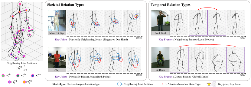
Figure 1: SkateFormer’s partition-specific attention strategy for skeleton-based action recognition, leveraging two skeletal relation types – physically neighboring and distant joints – and two temporal relation types for local and global motion.

The joints and their connections (or bones) in skeleton input correspond to the vertices and edges, respectively, in a graph structure. Consequently, many methods based on Graph Convolutional Networks (GCNs) [18] suitable for processing graph inputs have been extensively proposed for human action recognition. Most of the GCN-based methods [43, 24, 5, 67, 4, 36, 10, 6, 47, 19, 20, 46, 68, 75, 63, 22, 21, 61] exchange information between different joints within a single frame using graph convolutions, and capture the temporal dynamics for each joint using 1D temporal convolutions. However, they struggle to capture the relation of physically distant joints (e.g., between two hands with open arms) effectively due to the direct propagation of information between physically connected joints.

To mitigate this limitation, transformer-based methods utilizing self-attention to capture relations across all joint pairs have been proposed [40, 58, 60, 64]. Yet, considering every joint in every frame is inefficient as specific joints in certain frames are more critical for particular action recognition. Some transformer-based methods have tried to reduce computational complexity by squeezing features along the joint or frame dimension before self-attention [11], only using either skeletal or temporal relations [73, 44, 38, 13, 76], or by tokenizing physically similar skeletal information [34, 62]. Separating joints and frames during self-attention can obscure the critical skeletal-temporal relations for action recognition, and tokenization may dilute vital information, potentially degrading performance.

To overcome these issues, we propose an efficient transformer-based approach, called Skeletal-Temporal Transformer (SkateFormer) that introduces joint and frame partition strategies and partition-specific self-attention based on types of skeletal-temporal relations (Skate-Type). Fig. 1 illustrates the joint and frame partition strategies and partition-specific self-attention of our SkateFormer. For example, in the ‘make ok sign’ action class, relations between physically neighboring joints (e.g., joints on the same hand) are crucial, whereas in the ‘clap’ action class, relations between physically distant joints (e.g., between the palms of both hands) are more critical. Regarding temporal relations, for repetitive local motions like in the ‘brush teeth’ class, neighboring frame relations are essential, whereas for actions with global motion like ‘sit down’, distant frame relations become critical. Additionally, the speed at which actions are performed can vary significantly depending on the actor. To make our SkateFormer computationally efficient, we introduce a novel partition-specific attention (Skate-MSA). For this, we divide the skeletal-temporal relations into four partition types: (i) neighboring joints and local motion – Skate-Type-1, (ii) distant joints and local motion – Skate-Type-2, (iii) neighboring joints and global motion – Skate-Type-3 and (iv) distant joints and global motion – Skate-Type-4. Therefore, Skate-MSA is designed to efficiently capture skeletal-temporal relations at the joint-element-level, eliminating the need for tokenization, which typically involves joint-group-level attention [34, 62]. In summary, our contributions are as follows:

• We propose a Skeletal-Temporal Transformer (SkateFormer), a partition-specific attention strategy (Skate-MSA) for skeleton-based action recognition that captures skeletal-temporal relations and reduces computational complexity.

• We introduce a range of augmentation techniques and an effective positional embedding method, named Skate-Embedding, which combines skeletal and temporal features. This method significantly enhances action recognition performance by forming an outer product between learnable skeletal features and fixed temporal index features.

• Our SkateFormer sets a new state-of-the-art for action recognition performance across multiple modalities (4-ensemble condition) and single modalities (joint, bone, joint motion, bone motion), showing notable improvement over the most recent state-of-the-art methods. Additionally, it concurrently establishes a new state-of-the-art in interaction recognition, a sub-field of action recognition.

2 Related Works

2.1 RNN/CNN-based approaches

Recently, skeleton-based action recognition has made significant progress. Early research efforts focused on utilizing Recurrent Neural Networks (RNNs), including LSTM and GRU, to handle skeleton data due to its sequential and continuous nature [25, 37, 77, 28, 71, 45, 29]. Furthermore, some studies explored the conversion of skeleton data into pseudo-images to leverage Convolutional Neural Networks (CNNs) [59, 8, 66, 23, 17, 65]. Very recently, PoseC3D [12] employed a 2D pose estimation network [50] on RGB video to generate image-like skeleton heatmaps as input for CNNs, and Ske2Grid [1] proposed a method to transform 2D/3D skeleton data nodes into image-format grid patches.

2.2 GCN-based approaches

Skeleton data is composed of joints and bones, which correspond to vertices and edges in a graph. Consequently, research in this domain has predominantly gravitated towards Graph Neural Networks (GNNs) [42, 69] and Graph Convolutional Networks (GCNs) [43, 24, 5, 19, 20, 3, 4, 36, 10, 46, 6, 68, 47, 67, 21, 61]. InfoGCN [7] introduced additional loss terms to form a compact latent feature space, resulting in clear decision boundaries. Similarly, FR-Head [75] incorporated contrastive learning to separate feature representations of ambiguous classes. LST [63] introduced language supervision to train GCNs effectively, while HD-GCN [22] introduced rooted trees as a data structure to create diverse connections between joints. Despite their merits, GCNs have limitations in effectively capturing topology variations depending on the input data by using the fixed-sized kernels.

2.3 Transformer-based approaches

Recent research explores transformer-based approaches for skeleton-based action recognition, which excel in capturing data-adaptive joint connections [40, 58, 60, 64]. However, these methods often require high computational costs due to the usage of their large-sized attention maps. Early methods have tried to reduce attention map sizes by employing feature pooling [11] or reshaping [44] techniques. Some studies have attempted to mitigate computational load by utilizing separate skeletal and temporal attention modules in a parallel [73, 38] or serial [44, 76, 13] configurations. Nevertheless, they face challenges in simultaneously capturing skeletal-temporal relations, which are critical aspects of skeleton-based action recognition. IGFormer [34] and ISTA-Net [62] tackle the challenge by embedding joint sets within the same partition into a unified token before attention modules, relying solely on partition strategies for tokenization without introducing partition-specific attention mechanisms. Despite incorporating skeletal-temporal attention at the joint-group-level, they encounter limitations in local action recognition due to the tokenization process leading to the loss of physically similar skeletal information. In our work, the proposed SkateFormer employs partition-specific skeletal-temporal attention modules to effectively capture skeletal-temporal relations at the joint-element-level without tokenization.

Complexity of transformer-based vision tasks. Vision Transformers (ViT) [9] revolutionized the field of computer vision but face challenges due to high computational costs. To mitigate these challenges, various studies have been conducted to reduce the size of attention maps while efficiently propagating local and global information [30, 54]. In the context of vision tasks, 2D feature maps are organized along horizontal and vertical spatial axes. In contrast, our task involves skeletal and temporal axes, making the nature of our data fundamentally different. However, the elements within skeleton data tend to scale mostly with the factors such as the number of recognized joints, the number of individuals performing actions, and the number of frames, necessitating the reduction of computational complexity. Inspired by the works [53, 54], we propose a transformer structure that efficiently captures skeletal-temporal relations at the joint-element-level, reducing the computational cost.

3 Methodology

3.1 Overview of SkateFormer

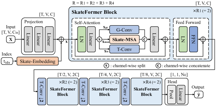
Figure 2: The overall framework of our proposed SkateFormer.

The overall architecture of our proposed SkateFormer is depicted in Fig. 2. A skeleton sequence, corresponding to a single action, is sampled to maintain a consistent frame count of $T$, resulting in $\mathbf{X}\in\mathbb{R}^{T\times V\times M\times C_{\mathsf{in}}}$, where $V$ represents the number of joints per frame, $M$ denotes the number of individuals involved in the action, and $C_{\mathsf{in}}$ is the dimensionality of data representing a single joint ($C_{\mathsf{in}}=3$ for 3D skeletons in our cases). Initially, we reshape $\mathbf{X}$ from $(T,V,M,C_{\mathsf{in}})$ to $(T,V{\cdot}M,C_{\mathsf{in}})$ to treat joints from different individuals separately. For simplicity, we redefine $V$ as $V{\cdot}M$ so that we have $\mathbf{X}\in\mathbb{R}^{T\times V\times C_{\mathsf{in}}}$ in subsequent text. Next, the three linear layers in the SkateFormer map the low-dimensional raw skeleton data into a higher-dimensional feature space. We then perform the skeletal-temporal positional embedding by adding learnable skeletal features and fixed temporal index features to this mapped feature. The embedded features pass through $R$ SkateFormer blocks, each comprising a self-attention layer that propagates features via skeletal-temporal relations, followed by a feed-forward layer that refines the features. The final features, after $R$ SkateFormer Blocks, undergo skeletal-temporal pooling to produce the outcome $\hat{\mathbf{y}}\in\mathbb{R}^{N_{c}}$, which is trained via backpropagation through a loss function by comparing $\hat{\mathbf{y}}$ with the true label $\mathbf{y}$, where $N_{c}$ represents the number of classes.

3.2 SkateFormer Block

Each of the SkateFormer Blocks in Fig. 2 is structured similarly as the traditional transformer blocks [30, 54], incorporating both a self-attention layer and a feed-forward network (FFN). The self-attention component of the SkateFormer Block can be expressed as follows:

$$\begin{split}&[\mathbf{x}_{\mathsf{gc}},\mathbf{x}_{\mathsf{tc}},\mathbf{x}_{\mathsf{msa}}]=\mathsf{Split}(\mathsf{Linear}(\mathsf{LN}(\mathbf{x})))\\ &\mathbf{x}_{\mathsf{gc}}\leftarrow\mathsf{G{\text{-}}Conv}(\mathbf{x}_{\mathsf{gc}})\\ &\mathbf{x}_{\mathsf{tc}}\leftarrow\mathsf{T{\text{-}}Conv}(\mathbf{x}_{\mathsf{tc}})\\ &\mathbf{x}_{\mathsf{msa}}\leftarrow\mathsf{Skate{\text{-}}MSA}(\mathbf{x}_{\mathsf{msa}})\\ &\mathbf{x}\leftarrow\mathbf{x}+\mathsf{Linear}(\mathsf{Concat}(\mathbf{x}_{\mathsf{gc}},\mathbf{x}_{\mathsf{tc}},\mathbf{x}_{\mathsf{msa}})),\end{split}$$ (1)

where the $\mathsf{LN}$ represents the Layer Normalization layer, the $\mathsf{Linear}$ denotes a fully-connected layer, and the $\mathsf{Split}$ indicates a channel splitting function. When input $\mathbf{x}$ to the self-attention component has $C$ channels, we split $\mathbf{x}$ into $\mathbf{x}_{\mathsf{gc}}$ of $C/4$ channels, $\mathbf{x}_{\mathsf{tc}}$ of $C/4$ channels, and $\mathbf{x}_{\mathsf{msa}}$ of $C/2$ channels. To obtain inductive biases for both skeletal and temporal aspects, we utilize a one-layer GCN ($\mathsf{G{\text{-}}Conv}$) and a single temporal convolution layer ($\mathsf{T{\text{-}}Conv}$), respectively. With a total of $H$ heads, we employ a learnable matrix of shape $(H/4,V,V)$ instead of a predefined adjacency matrix to perform $\mathsf{G{\text{-}}Conv}$ operations, enabling us to capture diverse connectivity patterns between joints. $\mathsf{T{\text{-}}Conv}$ is a 1D convolution layer with a kernel size of $k$, and performs 1D ($H/4$-group) convolutions for $\mathbf{x}_{\mathsf{tc}}$ to capture temporal dynamics. The FFN of the SkateFormer Block is expressed as follows: $\mathbf{x}\leftarrow\mathbf{x}+\mathsf{Linear}(\mathsf{Act}(\mathsf{Linear}(\mathsf{LN}(\mathbf{x}))))$, where $\mathsf{Act}$ represents the activation layer. When downsampling is needed for the input to a SkateFormer Block, a 1D convolution with a stride of 2 and Batch Normalization layer are applied.

3.3 Skate-MSA

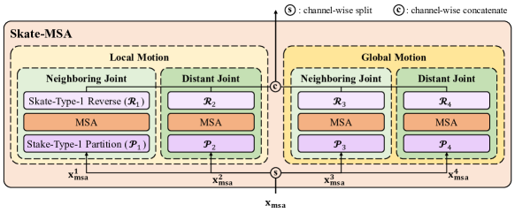
Figure 3: The Skate-MSA of our proposed SkateFormer.

As shown in Fig. 3, the feature map input $\mathbf{x}_{\mathsf{msa}}$ to the Skate-MSA is first split channel-wise into four equal-sized features $\mathbf{x}_{\mathsf{msa}}^{1},\mathbf{x}_{\mathsf{msa}}^{2},\mathbf{x}_{\mathsf{msa}}^{3},\mathbf{x}_{\mathsf{msa}}^{4}$, each of which has $C/8$ channels. For each $\mathbf{x}_{\mathsf{msa}}^{i}$, self-attention operation is applied to discern the correlations between joints corresponding to specific relation types as:

$$\begin{split}&\mathbf{x}_{\mathsf{msa}}^{i}\leftarrow\bm{\mathcal{R}}_{i}(\mathsf{MSA}(\bm{\mathcal{P}}_{i}(\mathbf{x}_{\mathsf{msa}}^{i})))\\ &\mathbf{x}_{\mathsf{msa}}\leftarrow\mathsf{Concat}(\mathbf{x}_{\mathsf{msa}}^{1},\mathbf{x}_{\mathsf{msa}}^{2},\mathbf{x}_{\mathsf{msa}}^{3},\mathbf{x}_{\mathsf{msa}}^{4}),\end{split}$$ (2)

where $\bm{\mathcal{P}}_{i}$ and $\bm{\mathcal{R}}_{i}$ represent the $i$-th Skate-Type partition and reverse operations, respectively. This approach enables the Skate-MSA to effectively analyze and model various joint relations in a specialized manner, contributing to its overall performance improvement.

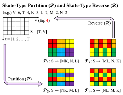
Figure 4: Skate-Type partition and reverse.

Partition and Reverse. Let a frame be $\mathbf{f}^{t}\in\mathbb{R}^{V\times C_{\mathsf{in}}}$ at time $t$. So, we have $\mathbf{X}=\{\mathbf{f}^{t}\}_{t=1}^{T}\in\mathbb{R}^{T\times V\times C_{\mathsf{in}}}$ where $\mathbf{f}^{t}$ consists of the 3D ($C_{\mathsf{in}}=3$) positions of $V$ joints at time $t$. The frames of $\mathbf{X}$ are often temporally highly correlated for most of the action types. However, the joint positions of skeletons tend to be less correlated among some joints, depending on different action types. Nevertheless, some other joints such as the joints of the head, neck, shoulders, abdomen and pelvises are relatively not highly variant among themselves for various action types. That is, they may move together in a group. So, it is efficient to partition the whole set of joints into smaller-sized joint partitions that can be useful to distinguish different actions. Furthermore, it is also worthwhile to consider categorizing the movements of various actions into two partitions, such as local and global motions: local motion, which only changes the positions of a small number of joints with partial movements such as teeth brushing and clapping, and global motion, which appears in the entire frames and includes actions like sitting down and standing up. Motivated from this, we partition the action into four skeletal-temporal relation types. For this, we first partition the entire set of joints into total non-overlapping $K$ subsets as neighboring joint partitions $\mathbf{v}_{k}^{\mathsf{njp}}$. For example, when $K=5$, we may have $\mathbf{v}_{1}^{\mathsf{njp}}$, $\mathbf{v}_{2}^{\mathsf{njp}}$, $\mathbf{v}_{3}^{\mathsf{njp}}$, $\mathbf{v}_{4}^{\mathsf{njp}}$ and $\mathbf{v}_{5}^{\mathsf{njp}}$ as the right arm, left arm, right leg, left leg and torso, respectively. The elements within each subset are ordered in a manner that extends outward from the body’s central region (e.g., for $k=3$, $v_{3,1}$, $v_{3,2}$ and $v_{3,3}$ are the 3D coordinates of the pelvis, right knee and right foot positions, respectively):

$$\mathbf{v}_{k}^{\mathsf{njp}}=[v_{k,1},v_{k,2},...,v_{k,L}],\\$$ (3)

where $k=1,2,...,K$, $L$ represents the total number of its elements, and $\mathbf{v}_{i}^{\mathsf{njp}}\cap\mathbf{v}_{j}^{\mathsf{njp}}=\varnothing$ for $i\neq j$. We stack $\mathbf{v}_{k}^{\mathsf{njp}}$’s, thus creating the skeletal axis as:

$$\mathbf{v}=\left[\mathbf{v}_{1}^{\mathsf{njp}}|\mathbf{v}_{2}^{\mathsf{njp}}|\cdots|\mathbf{v}_{K}^{\mathsf{njp}}\right],\\$$ (4)

where $|\mathbf{v}|=KL=V$. Also, to consider the relations between the joints that can be physically separated in a distance each other, we group the same-positioned elements of $\mathbf{v}_{k}^{\mathsf{njp}}$ to create possibly distant joint partitions $\mathbf{v}_{l}^{\mathsf{djp}}$ as:

$$\mathbf{v}_{l}^{\mathsf{djp}}=[v_{1,l},v_{2,l},...,v_{K,l}],$$ (5)

where $l=1,2,...,L$. Similarly, we define $\mathbf{t}=\left[1,2,...,T\right]$ as a time axis. We further define two semantic time axes as $\mathbf{t}_{m}^{\mathsf{local}}$ for local motion comprehension and $\mathbf{t}_{n}^{\mathsf{global}}$ for global motion understanding as:

$$\begin{split}&\mathbf{t}_{m}^{\mathsf{local}}=\left[(m-1)N+1,(m-1)N+2,...,mN\right]\\ &\mathbf{t}_{n}^{\mathsf{global}}=\left[n,n+N,...,n+(M-1)N\right],\\ \end{split}$$ (6)

where $m=1,2,...,M$ with the total $M$ number of $\mathbf{t}_{n}^{\mathsf{global}}$ elements, and $n=1,2,...,N$ with the total $N$ number of $\mathbf{t}_{m}^{\mathsf{local}}$ elements. Note that $\mathbf{t}_{m}^{\mathsf{local}}$ is a segment of consecutive time indices to represent a local motion within the time segment while $\mathbf{t}_{n}^{\mathsf{global}}$ is an $N$-strided sparse time axis to capture the global motion over $\mathbf{t}$. So, we have $\mathbf{t}=\{\mathbf{t}_{m}^{\mathsf{local}}\}_{m=1}^{M}=\{\mathbf{t}_{n}^{\mathsf{global}}\}_{n=1}^{N}$ and $|\mathbf{t}|=MN=T$. Based on these time axes, our skeletal-temporal partitions of joints and frames are explained in the followings.

We partition the joints and frames together into four types in the context of skeletal-temporal relation for the Skate-MSA – Skate-Type-1, -2, -3 and -4: (i) The Skate-Type-1 partition, denoted as $\bm{\mathcal{P}}_{1}$, pertains to a self-attention branch targeting neighboring joints and local motion, based on $\mathbf{v}_{k}^{\mathsf{njp}}$ and $\mathbf{t}_{m}^{\mathsf{local}}$; (ii) the Skate-Type-2 partition $(\bm{\mathcal{P}}_{2})$ represents a branch for distant joints and local motion, based on $\mathbf{v}_{l}^{\mathsf{djp}}$ and $\mathbf{t}_{m}^{\mathsf{local}}$; (iii) the Skate-Type-3 partition $(\bm{\mathcal{P}}_{3})$ signifies a branch for neighboring joints and global motion, based on $\mathbf{v}_{k}^{\mathsf{njp}}$ and $\mathbf{t}_{n}^{\mathsf{global}}$; (iv) Lastly, the Skate-Type-4 partition $(\bm{\mathcal{P}}_{4})$ corresponds to a branch targeting distant joints and global motion, based on $\mathbf{v}_{l}^{\mathsf{djp}}$ and $\mathbf{t}_{n}^{\mathsf{global}}$. The Skate-Type partition operations transform the shape $(S=(T,V,c))$ of $\mathbf{x}_{\mathsf{msa}}^{i}$ into:

$$\begin{split}\bm{\mathcal{P}}_{1}:S&\rightarrow(MK,N,L,c)\quad\bm{\mathcal{P}}_{2}:S\rightarrow(ML,N,K,c)\\ \bm{\mathcal{P}}_{3}:S&\rightarrow(NK,M,L,c)\quad\bm{\mathcal{P}}_{4}:S\rightarrow(NL,M,K,c),\end{split}$$ (7)

where $c=C/8$. The partitioned feature map $\mathbf{x}_{\mathsf{msa}}^{i,\bm{\mathcal{P}}}=\bm{\mathcal{P}}_{i}(\mathbf{x}_{\mathsf{msa}}^{i})$ undergoes multi-head self-attention ($\mathsf{MSA}$) and is then reshaped back to its original size of $(T,V,c)$ through a Skate-Type reverse operation $\bm{\mathcal{R}}_{i}$ according to Eq. 2.

Multi-head self-attention. In order to collectively consider the skeletal-temporal relation types, we can generalize feature maps $\mathbf{x}_{\mathsf{msa}}^{i,\bm{\mathcal{P}}}$ to have a shape of $(B,T^{\prime},V^{\prime},c)$. The feature maps are first reshaped into $(B,T^{\prime}{\cdot}V^{\prime},c)$. Through linear mappings of $\mathbf{x}_{\mathsf{msa}}^{i,\bm{\mathcal{P}}}$ of shape $(c,c)$ by $\mathbf{W}_{Q}$, $\mathbf{W}_{K}$, and $\mathbf{W}_{V}$, we obtain the query ($\mathbf{Q}$), key ($\mathbf{K}$), and value ($\mathbf{V}$) tensors as $[\mathbf{Q},\mathbf{K},\mathbf{V}]=\mathbf{x}_{\mathsf{msa}}^{i,\bm{\mathcal{P}}}\cdot[\mathbf{W}_{Q},\mathbf{W}_{K},\mathbf{W}_{V}]$.

Since we utilized half of the total $H$ heads for $\mathsf{G{\text{-}}Conv}$ and $\mathsf{T{\text{-}}Conv}$ operations, the remaining $H/2$ heads are divided into quarters with $H^{\prime}=H/8$. They are then assigned differently with the four Skate-Types, each of which has a $\mathsf{MSA}$. We reshaped $\mathbf{Q}$, $\mathbf{K}$, $\mathbf{V}$ to have a shape of $(B,H^{\prime},T^{\prime}{\cdot}V^{\prime},c/H^{\prime})$. This refers to the self-attention ($\mathsf{SA}$) for each individual head $h$, given as:

$$\begin{split}&\mathsf{SA}_{h}(\mathbf{x}_{\mathsf{msa}}^{i,\bm{\mathcal{P}}})=\mathsf{SoftMax}(\mathbf{Q}_{h}\mathbf{K}_{h}^{\mathsf{T}}/\sqrt{c/H^{\prime}}+\mathbf{B}_{h})\mathbf{V}_{h}\\ &\mathsf{MSA}(\mathbf{x}_{\mathsf{msa}}^{i,\bm{\mathcal{P}}})=\mathsf{Concat}(\mathsf{SA}_{1}(\mathbf{x}_{\mathsf{msa}}^{i,\bm{\mathcal{P}}}),...,\mathsf{SA}_{H^{\prime}}(\mathbf{x}_{\mathsf{msa}}^{i,\bm{\mathcal{P}}})),\end{split}$$ (8)

where $\mathbf{Q}_{h}\mathbf{K}_{h}^{\mathsf{T}}$ is a data-dependent term that varies based on the input, and $\mathbf{B}_{h}$ represents the skeletal-temporal positional bias. To account for the characteristics of the temporal axis $\mathbf{t}$, we applied 1D relative positional bias: $\mathbf{B}_{h}^{\mathbf{t}}\in\mathbb{R}^{T^{\prime}\times T^{\prime}}$ [30] for the temporal splits, $\mathbf{t}_{m}^{\mathsf{local}}$ and $\mathbf{t}_{n}^{\mathsf{global}}$ in Eq. 6. Regarding the skeletal axis $\mathbf{v}$, for the skeletal split $\mathbf{v}_{k}^{\mathsf{njp}}$ in Eq. 3, due to the inconsistency between joints at the same position across partitions, no additional positional bias was applied: $\mathbf{B}_{h}^{\mathbf{v}}=\mathbbm{1}^{V^{\prime}\times V^{\prime}}$. For the skeletal split $\mathbf{v}_{l}^{\mathsf{djp}}$ in Eq. 5, where elements at the same position always represent a consistent semantic part of the body, we utilized absolute positional bias: $\mathbf{B}_{h}^{\mathbf{v}}\in\mathbb{R}^{V^{\prime}\times V^{\prime}}$. The skeletal-temporal positional bias $\mathbf{B}_{h}$ is: $\mathbf{B}_{h}=\mathbf{B}_{h}^{\mathbf{t}}\otimes\mathbf{B}_{h}^{\mathbf{v}}\in\mathbb{R}^{T^{\prime}V^{\prime}\times T^{\prime}V^{\prime}}$, where $\otimes$ is a Kronecker product.

Complexity analysis. The computational complexity of a naive self-attention layer [55, 9] for feature map $\mathbf{x}_{\mathsf{msa}}$ with a shape of $(T,V,C/2)$ is $2(VT)^{2}(C/2)$. In contrast, the computation complexity of our Skate-MSA is:

$$2(VT)^{2}\frac{C}{2}\left[\frac{1}{4}\left(\frac{1}{MK}+\frac{1}{ML}+\frac{1}{NK}+\frac{1}{NL}\right)\right].$$ (9)

In our experimental settings, this results in approximately a 48$\times$ reduction in computational complexity compared to the naive self-attention layer.

3.4 Skeletal-Temporal Positional Embedding

Our novel skeletal-temporal positional embedding method, called Skate-Embedding, is tightly associated with temporal data augmentation. So, we first explain data augmentation with our contribution and then describe the Skate-Embedding.

Intra-instance augmentation. We define intra-instance augmentation as data augmentation within each frame sequence. To ensure stable training of transformer-based models that require a substantial amount of data, we employed various data augmentation techniques. Previous skeleton-based action recognition methods often used data augmentation by temporally sampling input frames with fixed strides or randomly for the whole input, which we refer to as temporal augmentation. Also, as skeletal augmentation, various transformations such as the actor order permutation, random shear, random rotation, random scaling, random coordinate drop, and random joint dropout etc. have been applied [26, 14].

We propose trimmed-uniform random sampling of frames with $p$ portion. This sampling cuts out the first and last parts of the total input sequence and performs uniform random sampling of frames. Fig. 5 illustrates our trimmed-uniform random sampling of frames with $p$ portion. From our trimmed-uniform random sampling of frames with a $p$ portion, the masking effect of skeleton sequences in their front and back portions, as well as a more dense sampling effect in the middle, are expected. This can lead to a concentration in the middle portion, resulting in better data augmentation.

Inter-instance augmentation. We define inter-instance augmentation as data augmentation by exchanging the bone lengths of different subjects across different frame sequences (not within each frame sequence). By doing so, the resulting data augmentation can provide the diversity of subjects with different body sizes, which can help generalization learning.

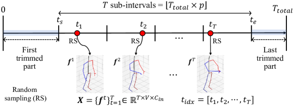
Figure 5: The proposed trimmed-uniform random sampling of frames with $p$ portion.

Skate-Embedding. We propose a novel skeletal-temporal positional embedding method, called Skate-Embedding, that utilizes fixed (not learnable) temporal index features and learnable (not fixed) skeletal features. The temporal index features are suitable for conveying to the first SkateFormer Block the temporal positional information of the sampled frames from sequences of various lengths. The sampled temporal indices are designated as $t_{\mathsf{idx}}=[t_{1},t_{2},...,t_{T}]$, as illustrated in Fig 5. These temporal indices are then normalized to the range $[-1,1]$, and are used for the fixed temporal index features as done in the temporal positional embedding. The fixed temporal index features, denoted as $\mathsf{TE}\in\mathbb{R}^{T\times C}$, are constructed for $t_{\mathsf{idx}}$ by using the sinusoidal positional embedding [55]. On the other hand, as skeletal joint positional (which are not the 3D coordinates of joints but their indices) embeddings, the learnable skeletal features, denoted as $\mathsf{SE}\in\mathbb{R}^{V\times C}$, are learned within the Skate-Embedding as shown in Fig. 2. Finally, the skeletal-temporal positional embedding $\mathsf{STE}\in\mathbb{R}^{T\times V\times C}$ is done by taking the outer product of $\mathsf{SE}$ and $\mathsf{TE}$ as $\mathsf{STE}[i,j,d]=\mathsf{SE}[j,d]\cdot\mathsf{TE}[i,d]$ at the $i$-th time, the $j$-th joint and the $d$-th channel.

4 Experimental Results

4.1 Datasets

NTU RGB+D. This dataset [41] offers 60 action classes and includes diverse activities like drinking water, eating, brushing teeth, dropping objects, and more. It comprises total 56,880 videos captured from 40 subjects across 155 camera viewpoints. The dataset utilizes Kinect v2, encompassing RGB, IR, depth, and 3D skeleton data, and supports cross-subject (X-Sub60) and cross-view (X-View60) evaluation. Out of the 60 action classes, only 11 are related to human interaction, specifically when two individuals are present. We denote this subset as NTU-Inter [34, 11].

NTU RGB+D 120. This dataset [27] extends the NTU RGB+D dataset [41] with 120 action classes, covering actions such as putting on headphones, basketball shooting, juggling table tennis balls, and more. It contains 114,480 videos from 106 subjects across 155 camera viewpoints. It enables cross-subject (X-Sub120) and cross-setup (X-Set120) evaluation based on different subject and camera setups. Out of the 120 action classes, only 26 are related to human interaction. We denote this subset as NTU-Inter 120 [34, 11, 62].

NW-UCLA. This dataset [56] includes 10 action classes, such as picking up objects, dropping trash, walking, sitting, standing, and more. It comprises total 1,475 videos from 10 subjects across three camera views, collected using Kinect v1 [74] and featuring RGB, IR, depth, and 3D skeleton data. Evaluation follows the cross-view approach, utilizing two training views and one test view.

4.2 Experiment Details

All experiments were performed using the PyTorch framework [35], running on a single NVIDIA DGX A100 GPU. Each model was trained with a total of 500 epochs. We employed a linear warm-up strategy for the learning rate, gradually increasing it from $10^{-7}$ to $10^{-3}$ during the first 25 epochs. Subsequently, a cosine-annealing scheduler [31] was used to update the learning rate at each iteration for the remaining epochs. We employed the AdamW optimizer [32] with a betas of (0.9, 0.999), a weight decay of $5\times 10^{-4}$. Additionally, gradient clipping [70] was applied for the loss values with gradients exceeding 1. The batch size was set to 128, the random seed was fixed at 1, and we adopted the label-smoothed cross-entropy loss [52, 33] as our loss function with parameter $\alpha=0.1$.

From various experiments, we found the empirical values as follows. For our experiments with the NTU RGB+D and NTU RGB+D 120 datasets, we used the following configuration: $V=48$ (excluding the center of the body, resulting in 24 joints for each of the two individuals), $T=64$, $L=4$, $K=12$, $M=8$, $N=8$, and $C=96$. For the experiments with the NW-UCLA dataset, $V=20$, $T=64$, $L=4$, $K=5$, $M=8$, $N=8$, and $C=96$. Furthermore, we employed a total of $R=8$ SkateFormer Blocks, applying temporal downsampling after every 2 blocks. The kernel size for the $\mathsf{T{\text{-}}Conv}$ layers was set to $k=7$. For the performance evaluation, we compare our SkateFormer with other methods in terms of the top-1 action recognition accuracy for the test data sets.

4.3 Performance Comparison

We present a comprehensive performance comparison for our SkateFormer against recent state-of-the-art skeleton-based action recognition methods. The performance comparison is made for three ensembles of different modalities ($\mathbb{E}_{1}$, $\mathbb{E}_{2}$, $\mathbb{E}_{4}$): (i) $\mathbb{E}_{1}$ - joint modality only; (ii) $\mathbb{E}_{2}$ - joint + bone modalities; and (iii) $\mathbb{E}_{4}$ - joint + bone + joint motion + bone motion modalities. As in [7, 75, 3, 76], we train separate networks for each modality and ensemble their outputs. Table 1 shows the overall performance comparisons of various methods for the NTU RGB+D, NTU RGB+D 120 and NW-UCLA datasets under the three ensembles. Notably, several works address human interaction recognition [34, 62, 11], a sub-part of skeleton-based action recognition, specifically focusing on scenarios where two or more individuals coexist within a single action. Accordingly, we additionally present the performance of human interaction recognition methods on the NTU Inter and NTU Inter 120 datasets in Table 2.

Table 1: Top-1 accuracy of different skeleton-based action recognition methods on the NTU RGB+D, NTU RGB+D 120 and NW-UCLA datasets. The methods of RNN, CNN, GCN, and Transformer types are evaluated based on the number of input frames and the use of ensemble strategies. The best performances are highlighted in bold.

Types	Methods	Frames	NTU RGB+D (%)						NTU RGB+D 120 (%)						NW-UCLA (%)
			X-Sub60			X-View60			X-Sub120			X-Set120
			$\mathbb{E}_{1}$	$\mathbb{E}_{2}$	$\mathbb{E}_{4}$	$\mathbb{E}_{1}$	$\mathbb{E}_{2}$	$\mathbb{E}_{4}$	$\mathbb{E}_{1}$	$\mathbb{E}_{2}$	$\mathbb{E}_{4}$	$\mathbb{E}_{1}$	$\mathbb{E}_{2}$	$\mathbb{E}_{4}$
RNN	AGC-LSTM [45]	100	87.5	89.2	-	93.5	95.0	-	-	-	-	-	-	-	93.3
CNN	TA-CNN [65]	64	88.8	-	90.4	93.6	-	94.8	82.4	-	85.4	84.0	-	86.8	96.1
	Ske2Grid [1]	100	88.3	-	-	95.7	-	-	82.7	-	-	85.1	-	-	-
GCN	SGN [72]	20	-	89.0	-	-	94.5	-	-	79.2	-	-	81.5	-	-
	CTR-GCN [3]	64	89.9	-	92.4	-	-	96.8	84.9	88.7	88.9	-	90.1	90.6	96.5
	ST-GCN++ [10]	100	89.3	91.4	92.1	95.6	96.7	97.0	83.2	87.0	87.5	85.6	87.5	89.8	-
	InfoGCN [7]	64	-	-	92.7	-	-	96.9	85.1	88.5	89.4	86.3	89.7	90.7	96.6
	FR-Head [75]	64	90.3	92.3	92.8	95.3	96.4	96.8	85.5	-	89.5	87.3	-	90.9	96.8
	Koopman [61]	64	90.2	-	92.9	95.2	-	96.8	85.7	-	90.0	87.4	-	91.3	97.0
	LST [63]	64	90.2	-	92.9	95.6	-	97.0	85.5	-	89.9	87.0	-	91.1	97.2
	HD-GCN [22]	64	90.6	92.4	93.0	95.7	96.6	97.0	85.7	89.1	89.8	87.3	90.6	91.2	96.9
	STC-Net [21]	64	-	92.5	93.0	-	96.7	97.1	-	89.3	89.9	-	90.7	91.3	97.2
Trans- former	DSTA-Net [44]	128	-	-	91.5	-	-	96.4	-	-	86.6	-	-	89.0	-
	STST [73]	128	-	-	91.9	-	-	96.8	-	-	-	-	-	-	-
	FG-STFormer [13]	128	-	-	92.6	-	-	96.7	-	-	89.0	-	-	90.6	97.0
	Hyperformer [76]	64	90.7	-	92.9	95.1	-	96.5	86.6	-	89.9	88.0	-	91.3	96.7
	SkateFormer	64	92.6	93.0	93.5	97.0	97.4	97.8	87.7	89.4	89.8	89.3	91.0	91.4	98.3

$\mathbb{E}_{1}$, $\mathbb{E}_{2}$, $\mathbb{E}_{4}$ performance. As shown in Tables 1,  2, the extensive experiments demonstrate that our SkateFormer outperforms all the state-of-the-art (SoTA) methods except the $\mathbb{E}_{4}$ of X-Sub120. It should be noted that the performance of our SkateFormer is relatively higher for $\mathbb{E}_{1}$ and $\mathbb{E}_{2}$ than $\mathbb{E}_{4}$. This is indicative of the model’s efficient attention strategy, which is based on partition-specific processing, allowing for the simultaneous handling of joint (input), bone (skeletal relations), joint motion (temporal relations), and bone motion (skeletal-temporal relations) inputs within a singular network framework. As the ensemble modality increases, the potential for information redundancy also rises, which may diminish the ensemble synergy. Therefore, our SkateFormer is already somewhat a strong learner in the form of a single modality compared to others.

Ensemble methods improve performance, but their effectiveness depends on the computational complexity, scaling proportionally with the number of models in the ensemble. Also, optimizing ensemble coefficients is dataset and model-specific [22], posing challenges in real-world applications. Consequently, it is crucial to leverage diverse modalities inherently within a single model to achieve both generalization and efficiency. Therefore, highlighting the importance of $\mathbb{E}_{1}$ performance is essential as a key indicator of the model’s ability to generalize across diverse inputs.

Table 2: Comparison with human interaction recognition methods on the NTU-Inter and NTU-Inter 120 datasets. The best performances are highlighted in bold.

Types	Methods	NTU-Inter ($\mathbb{E}_{1}$, %)		NTU-Inter 120 ($\mathbb{E}_{1}$, %)		Params. (M)	FLOPs (G)	Time (ms)
		X-Sub60	X-View60	X-Sub120	X-Set120
Transformer	IGFormer [34]	93.6	96.5	85.4	86.5	-	-	-
	SkeleTR [11]	94.9	97.7	87.8	88.3	3.82	7.30	-
	ISTA-Net [62]	-	-	90.6	91.7	6.22	68.18	21.71
	SkateFormer	97.1	99.3	92.3	93.2	2.02	3.62	11.25

Table 3: Comparative analysis of SkateFormer with other methods by parameters, FLOPs, inference time, and average top-1 accuracy for joint modality.

Types	Methods	Params. (M)	FLOPs (G)	Time (ms)	NTU RGB+D ($\mathbb{E}_{1}$, %)	NTU RGB+D 120 ($\mathbb{E}_{1}$, %)
GCN	InfoGCN [7]	1.56	3.34	12.97	-	85.7
	FR-Head [75]	1.45	3.60	18.49	92.8	86.4
	Koopman [61]	5.38	8.76	17.86	92.7	86.6
	LST [63]	2.10	3.60	18.85	92.9	86.3
	HD-GCN [22]	1.66	3.44	72.81	93.2	86.5
Transformer	DSTA-Net [44]	3.45	16.18	13.80	-	-
	Hyperformer [76]	2.71	9.64	18.07	92.9	87.3
	SkateFormer	2.03	3.62	11.46	94.8	88.5

Computational complexity analysis. Table 3 shows the complexity comparisons [48] for various skeleton-based action recognition methods. Our SkateFormer exhibits a competitive balance between model complexity and computational efficiency, compared to other methods. It maintains a comparable number of parameters and FLOPs with the GCN-based methods, while substantially reducing these metrics in comparison to the transformer-based counterparts. Table 3 has been compiled using publicly available official code.

4.4 Ablation Studies

To see the efficacy of the key components in our SkateFormer, the ablation experiments were carried for the NTU RGB+D dataset. A detailed analysis on the effectiveness of the components is provided in Tables 4, 6, 6 to quantify the impact of different design choices on the model’s performance in terms of accuracy (%) across two benchmarks: X-Sub60 and X-View60.

Skate-Types of Skate-MSA. Table 4 presents the impact of different Skate-Types on accuracy. As shown, incorporating the skeletal relation types only improves the action classification performance over the baseline, and so does the temporal relation types only. The full model that utilizes the Skate-Types (skeletal-temporal relation types) achieves the highest accuracy, indicating that both skeletal and temporal splits are crucial in distinguishing complex actions.

Table 4: Ablation study on the influence of skeletal and temporal relation types (SkateTypes) of Skate-MSA in our SkateFormer.

Relation Types	NTU RGB+D (%)		Params. (M)	FLOPs (G)	Time (ms)
	X-Sub60	X-View60
Baseline (only $\mathbf{V}_{h}$ in Eq. 8)	90.7	95.7	2.03	3.591	10.68
Baseline + $\mathbf{v}_{k}^{\mathsf{njp}}$ + $\mathbf{v}_{l}^{\mathsf{djp}}$ (skeletal)	91.8 ($\uparrow$1.1)	96.4 ($\uparrow$0.7)	2.03	3.594	11.10
Baseline + $\mathbf{t}_{m}^{\mathsf{local}}$ + $\mathbf{t}_{n}^{\mathsf{global}}$ (temporal)	91.9 ($\uparrow$1.2)	96.6 ($\uparrow$0.9)	2.03	3.593	11.09
Baseline + $\mathbf{v}_{k}^{\mathsf{njp}}$ + $\mathbf{v}_{l}^{\mathsf{djp}}$ + $\mathbf{t}_{m}^{\mathsf{local}}$ + $\mathbf{t}_{n}^{\mathsf{global}}$	92.6 ($\uparrow$1.9)	97.0 ($\uparrow$1.3)	2.03	3.620	11.46

Exploration of Skate-Embedding. Table 6 shows the ablation study on the $\mathsf{STE}$ to assess the impact of different skeletal and temporal embedding methods. We explore various combinations of skeletal and temporal embedding methods. The learnable skeletal embedding ($\mathsf{SE}$) paired with fixed temporal embedding ($\mathsf{TE}$) achieves superior performance, suggesting an optimal balance between adaptability and stability in embeddings. The Skate-Embedding allows for a more tailored feature representation, leading to improved recognition accuracy.

Table 5: Ablation study results on the Skate-Embedding to assess skeletal and temporal embedding impacts.

Embedding Methods				NTU RGB+D (%)
Skeletal	Temporal	X-Sub60	X-View60
✗	✗	91.9 ($\downarrow$0.7)	96.6 ($\downarrow$0.4)
	Learnable	91.8 ($\downarrow$0.8)	96.5 ($\downarrow$0.5)
	Fixed ($\mathsf{TE}$)	91.6 ($\downarrow$1.0)	96.6 ($\downarrow$0.4)
Learnable ($\mathsf{SE}$)	✗	92.1 ($\downarrow$0.5)	96.5 ($\downarrow$0.5)
	Learnable	91.4 ($\downarrow$1.2)	96.2 ($\downarrow$0.8)
	Fixed ($\mathsf{TE}$)	92.6	97.0

Table 6: Ablation study results on the effect of intra-instance and inter-instance augmentations.

Intra-instance					Inter-instance	NTU RGB+D (%)
Temporal	Skeletal		X-Sub60	X-View60
Trimmed			89.8	94.6
Trimmed		✓	90.3 ($\uparrow$0.5)	94.3 ($\downarrow$0.3)
Trimmed	✓		92.2 ($\uparrow$2.4)	96.6 ($\uparrow$2.0)
Fixed	✓	✓	91.4 ($\uparrow$1.6)	96.4 ($\uparrow$1.8)
Uniform	✓	✓	91.6 ($\uparrow$1.8)	96.8 ($\uparrow$2.2)
Trimmed	✓	✓	92.6 ($\uparrow$2.8)	97.0 ($\uparrow$2.4)

Evaluation of frame sampling methods. In Table 6, we compare three frame sampling strategies with (i) fix-strided (Fixed), (ii) uniform random (Uniform) and (iii) our trimmed-uniform random (Trimmed) sampling methods. Due to the masking effect of skeleton sequences in their front and the back portions as well and more dense sampling effect in the middles during training, the trimmed-uniform random sampling is more effective in perspectives of generalization learning and data augmentation. It surpasses traditional fix-strided and uniform random sampling approaches with 1.2 (0.6)% and 1.0 (0.2)% margins for the X-Sub60 (X-View60), respectively.

Impact of data augmentations. Table 6 presents the effectiveness of intra-instance (traditional) and inter-instance (additional) data augmentations. The intra-instance augmentation alone improves the performance while performance drop is observed with the inter-instance augmentation alone for the X-View60. This performance drop with 0.3%-point in accuracy is due to the inherent characteristics of the cross-view setting such that the variability in bone lengths across different subjects within the X-View60 is limited. This implies that the model may already encapsulate a comprehensive representation of these attributes. Consequently, the introduction of inter-instance data augmentation does not contribute additional discriminative information and may instead introduce redundancy, leading to a performance decline. However, the amalgamation of both intra- and inter-instance augmentations provides a synergistic enhancement, especially by random scaling and shearing on bone lengths in the skeletal augmentation, achieving peak accuracy of 92.6% on X-Sub60 and 97.0% on X-View60.

5 Conclusions

In this paper, we presented SkateFormer – a novel skeletal-temporal transformer tailored for action recognition tasks. For this, we propose an effective partition-specific attention strategy in skeleton-based action recognition, both to capture essential features and to reduce computational complexity. For efficient training, our novel Skate-Embedding that combines skeletal and temporal features is presented, significantly enhancing action recognition performance by forming an outer product between learnable skeletal features and fixed temporal index features. Our SkateFormer sets a new state-of-the-art for action recognition performance across multiple modalities (4-ensemble condition) and single modalities (joints, bones, joint motions, bone motions), showing notable improvement over the most recent state-of-the-art methods.

Appendix 0.A Discussion on Various Partition-Based Approaches

In recent studies, several partition-based methods such as DSTA-Net [44], ST-TR [38], IIP-Trnasformer [60], STST [73], FG-STFormer [13], Hyperformer [76], IGFormer [34], SkeleTR [11], and ISTA-Net [62] have been proposed. As shown in Table 7, we introduce SkateFormer, which differs fundamentally in the following aspects:

Table 7: Comparison with ours SkateFormer with existing transformer-based methods. S-Attn, T-Attn, T-Conv, and ST-Attn indicate ‘skeletal attention’, ‘temporal attention’, ‘temporal convolution’ and ‘skeletal-temporal attention’, respectively.

Tasks	Methods	Partition Types	Tokenization for Attention	Attention Types
Human Action Recognition	DSTA-Net [44]	N/A (Reshaping)	No	S-Attn, T-Attn (Sequential)
	ST-TR [38]	N/A (Reshaping)	No	S-Attn, T-Attn (Parallel)
	IIP-Transformer [60]	S-Type	Yes	S-Attn, T-Attn (Sequential)
	STST [73]	N/A (Reshaping)	No	S-Attn, T-Attn (Parallel)
	FG-STFormer [13]	S-Type	Yes	S-Attn, T-Attn (Sequential)
	Hyperformer [76]	S-Type	Yes	S-Attn, T-Conv (Sequential)
Human Interaction Recognition	IGFormer [34]	S-Type, T-Type	Yes	Joint-group-level ST-Attn
	SkeleTR [11]	N/A (Pooling)	Yes	Joint-group-level ST-Attn
	ISTA-Net [62]	S-Type, T-Type	Yes	Joint-group-level ST-Attn
Both	SkateFormer	4 Skate-Types	No	Joint-element-level ST-Attn

• Unlike existing methods that rely solely on physically neighboring joints (S-Type) or local motion (T-Type), our SkateFormer leverages four skeletal-temporal relation types (Skate-Types) with joint partitions (physically ‘neighboring’ + ‘distant’) and frame partitions (‘local’ + ‘global’ motions).

• While prior approaches typically tokenize joints within the same partition into a single feature (partition-based tokenization, not partition-specific attention), our SkateFormer adopts self-attention within each partition, enhancing its capability for fine-grained analysis.

• To mitigate computational complexity, existing methods often employ strategies such as conducting attention solely in the skeletal dimension while utilizing temporal convolution in the temporal dimension, or separately performing skeletal and temporal attention mechanisms, or employing joint-group-level attention with tokenization. In contrast, our SkateFormer is specifically designed to efficiently capture skeletal-temporal relations at the joint-element-level, thus eliminating the need for tokenization.

Appendix 0.B Additional Results

0.B.1 Recognition Accuracy based on Action Labels

Table 8 presents the top-1 accuracy results for single-joint modality (J) action recognition in the NTU RGB+D X-Sub60 evaluation, categorized by action labels. The baseline model represents a model without the application of partition-specific attention based on four skeletal-temporal relation types from Skate-MSA (only $\mathbf{V}_{h}$ in Eq. 8). The model denoted as (+ $\mathbf{v}_{k}^{\mathsf{njp}}$ + $\mathbf{v}_{l}^{\mathsf{djp}}$) applies partition-specific attention based on two skeletal relation types, while (+ $\mathbf{t}_{m}^{\mathsf{local}}$ + $\mathbf{t}_{n}^{\mathsf{global}}$) utilizes partition-specific attention based on two temporal relation types. The model labeled (+$\mathbf{v}_{k}^{\mathsf{njp}}$ + $\mathbf{v}_{l}^{\mathsf{djp}}$ + $\mathbf{t}_{m}^{\mathsf{local}}$ + $\mathbf{t}_{n}^{\mathsf{global}}$) represents the full SkateFormer model, which incorporates partition-specific attention based on four Skate-Types.

Our baseline model already outperforms state-of-the-art methods [67, 3, 10, 7, 75, 63, 22], as evident from the average top-1 accuracy. The Rank in the baseline indicates the ranking of top-1 accuracy among 60 classes. Comparing the full model to the baseline, we observed performance improvements in the majority of action labels (42 out of 60 classes), with eight classes maintaining the same performance, and a slight decrease in performance for ten classes. This can be interpreted as an effective utilization of limited model capacity, where slight decreases in performance for high-performing action labels (high-rank) allow for significant improvements in performance for lower-performing action labels (low-rank).

Notably, the baseline performance for actions such as ‘wear a shoe’ and ‘take off a shoe’ increased substantially from (60.81%, 78.83%) to (87.55%, 83.94%), demonstrating that our partition-specific attention enhances discriminative capability for similar classes. Furthermore, performance improvements for relatively low-rank action labels, such as ‘typing on a keyboard’, ‘sneeze/cough’, ‘use a fan (with hand or paper)/feeling warm’, were substantial.

Analysis of failure cases. As shown in Table 8, most of the failure cases occur when action classes are determined by fine finger motions, e.g. ‘reading’, ‘writing’, ‘playing with phone/tablet’, and ‘typing on a keyboard’.

Table 8: Top-1 accuracy based on action labels in NTU RGB+D X-Sub60 evaluation.

Action Label	Baseline (Rank)	+$\mathbf{v}_{k}^{\mathsf{njp}}$ + $\mathbf{v}_{l}^{\mathsf{djp}}$	+ $\mathbf{t}_{m}^{\mathsf{local}}$ + $\mathbf{t}_{n}^{\mathsf{global}}$	+$\mathbf{v}_{k}^{\mathsf{njp}}$ + $\mathbf{v}_{l}^{\mathsf{djp}}$ + $\mathbf{t}_{m}^{\mathsf{local}}$ + $\mathbf{t}_{n}^{\mathsf{global}}$
drink water	85.77 (47)	85.77 (–0.00)	85.77 (–0.00)	88.32 ($\uparrow$2.55)
eat meal/snack	76.00 (56)	77.82 ($\uparrow$1.82)	77.45 ($\uparrow$1.45)	78.18 ($\uparrow$2.18)
brushing teeth	90.11 (42)	85.35 ($\downarrow$4.76)	91.21 ($\uparrow$1.10)	89.01 ($\downarrow$1.10)
brushing hair	89.01 (45)	91.21 ($\uparrow$2.20)	93.77 ($\uparrow$4.76)	93.41 ($\uparrow$4.40)
drop	92.00 (39)	94.18 ($\uparrow$2.18)	92.36 ($\uparrow$0.36)	92.73 ($\uparrow$0.73)
pickup	97.09 (18)	97.82 ($\uparrow$0.73)	97.09 (–0.00)	98.55 ($\uparrow$1.45)
throw	92.73 (36)	93.45 ($\uparrow$0.73)	92.00 ($\downarrow$0.73)	93.82 ($\uparrow$1.09)
sitting down	98.17 (13)	98.53 ($\uparrow$0.37)	99.27 ($\uparrow$1.10)	98.53 ($\uparrow$0.37)
standing up (from sitting position)	98.90 (7)	98.53 ($\downarrow$0.37)	99.63 ($\uparrow$0.73)	98.90 (–0.00)
clapping	83.88 (51)	81.68 ($\downarrow$2.20)	86.08 ($\uparrow$2.20)	85.35 ($\uparrow$1.47)
reading	58.61 (60)	60.81 ($\uparrow$2.20)	61.54 ($\uparrow$2.93)	63.37 ($\uparrow$4.76)
writing	68.38 (57)	68.01 ($\downarrow$0.37)	66.91 ($\downarrow$1.47)	71.32 ($\uparrow$2.94)
tear up paper	95.94 (21)	96.68 ($\uparrow$0.74)	94.46 ($\downarrow$1.48)	95.94 (–0.00)
wear jacket	98.18 (12)	98.18 (–0.00)	98.55 ($\uparrow$0.36)	97.82 ($\downarrow$0.36)
take off jacket	98.19 (10)	98.91 ($\uparrow$0.72)	99.64 ($\uparrow$1.45)	99.64 ($\uparrow$1.45)
wear a shoe	60.81 (59)	86.81 ($\uparrow$26.01)	84.62 ($\uparrow$23.81)	87.55 ($\uparrow$26.74)
take off a shoe	78.83 (53)	82.48 ($\uparrow$3.65)	78.47 ($\uparrow$0.36)	83.94 ($\uparrow$5.11)
wear on glasses	93.04 (34)	93.41 ($\uparrow$0.37)	93.77 ($\uparrow$0.73)	93.41 ($\uparrow$0.37)
take off glasses	95.62 (23)	95.62 (–0.00)	95.26 ($\downarrow$0.36)	94.89 ($\downarrow$0.73)
put on a hat/cap	96.69 (19)	97.43 ($\uparrow$0.74)	98.16 ($\uparrow$1.47)	97.79 ($\uparrow$1.10)
take off a hat/cap	98.90 (7)	98.53 ($\downarrow$0.37)	98.90 (–0.00)	98.90 (–0.00)
cheer up	93.80 (29)	92.34 ($\downarrow$1.46)	93.80 (–0.00)	94.89 ($\uparrow$1.09)
hand waving	93.80 (29)	94.16 ($\uparrow$0.36)	93.80 (–0.00)	93.07 ($\downarrow$0.73)
kicking something	94.20 (27)	94.93 ($\uparrow$0.72)	97.10 ($\uparrow$2.90)	97.83 ($\uparrow$3.62)
reach into pocket	84.67 (49)	84.31 ($\downarrow$0.36)	86.13 ($\uparrow$1.46)	86.86 ($\uparrow$2.19)
hopping (one foot jumping)	98.91 (6)	98.91 (–0.00)	98.91 (–0.00)	98.91 (–0.00)
jump up	100.00 (1)	100.00 (–0.00)	100.00 (–0.00)	100.00 (–0.00)
make a phone call/answer phone	90.18 (41)	89.09 ($\downarrow$1.09)	90.55 ($\uparrow$0.36)	92.00 ($\uparrow$1.82)
playing with phone/tablet	76.36 (55)	76.36 (–0.00)	77.09 ($\uparrow$0.73)	74.91 ($\downarrow$1.45)
typing on a keyboard	64.36 (58)	72.73 ($\uparrow$8.36)	74.55 ($\uparrow$10.18)	77.82 ($\uparrow$13.45)
pointing to something with finger	79.71 (52)	88.04 ($\uparrow$8.33)	81.88 ($\uparrow$2.17)	84.42 ($\uparrow$4.71)
taking a selfie	92.39 (38)	93.84 ($\uparrow$1.45)	94.57 ($\uparrow$2.17)	93.12 ($\uparrow$0.72)
check time (from watch)	93.12 (33)	91.67 ($\downarrow$1.45)	92.75 ($\downarrow$0.36)	92.03 ($\downarrow$1.09)
rub two hands together	89.13 (43)	89.49 ($\uparrow$0.36)	91.30 ($\uparrow$2.17)	92.03 ($\uparrow$2.90)
nod head/bow	97.46 (14)	98.55 ($\uparrow$1.09)	98.55 ($\uparrow$1.09)	99.28 ($\uparrow$1.81)
shake head	94.55 (26)	95.27 ($\uparrow$0.73)	96.73 ($\uparrow$2.18)	96.00 ($\uparrow$1.45)
wipe face	85.87 (46)	87.32 ($\uparrow$1.45)	87.68 ($\uparrow$1.81)	90.94 ($\uparrow$5.07)
salute	93.48 (31)	93.48 (–0.00)	93.84 ($\uparrow$0.36)	94.93 ($\uparrow$1.45)
put the palms together	97.46 (14)	97.46 (–0.00)	96.74 ($\downarrow$0.72)	96.38 ($\downarrow$1.09)
cross hands in front (say stop)	96.01 (20)	97.10 ($\uparrow$1.09)	96.38 ($\uparrow$0.36)	97.46 ($\uparrow$1.45)
sneeze/cough	78.62 (54)	82.97 ($\uparrow$4.35)	83.33 ($\uparrow$4.71)	85.51 ($\uparrow$6.88)
staggering	99.28 (4)	99.64 ($\uparrow$0.36)	100.00 ($\uparrow$0.72)	99.28 (–0.00)
falling	99.64 (2)	100.00 ($\uparrow$0.36)	99.64 (–0.00)	100.00 ($\uparrow$0.36)
touch head (headache)	84.06 (50)	89.13 ($\uparrow$5.07)	84.06 (–0.00)	88.41 ($\uparrow$4.35)
touch chest (stomachache/heart pain)	93.84 (28)	94.57 ($\uparrow$0.72)	93.48 ($\downarrow$0.36)	96.01 ($\uparrow$2.17)
touch back (backache)	95.29 (24)	94.57 ($\downarrow$0.72)	95.29 (–0.00)	95.65 ($\uparrow$0.36)
touch neck (neckache)	90.22 (40)	90.58 ($\uparrow$0.36)	92.39 ($\uparrow$2.17)	93.12 ($\uparrow$2.90)
nausea or vomiting condition	85.45 (48)	83.64 ($\downarrow$1.82)	84.00 ($\downarrow$1.45)	85.45 (–0.00)
use a fan (with hand or paper)/feeling warm	89.09 (44)	90.91 ($\uparrow$1.82)	89.45 ($\uparrow$0.36)	94.18 ($\uparrow$5.09)
punching/slapping other person	92.70 (37)	93.07 ($\uparrow$0.36)	92.70 (–0.00)	94.16 ($\uparrow$1.46)
kicking other person	95.65 (22)	96.38 ($\uparrow$0.72)	95.65 (–0.00)	96.38 ($\uparrow$0.72)
pushing other person	98.55 (9)	97.83 ($\downarrow$0.72)	97.46 ($\downarrow$1.09)	98.19 ($\downarrow$0.36)
pat on back of other person	93.48 (31)	95.29 ($\uparrow$1.81)	94.93 ($\uparrow$1.45)	95.65 ($\uparrow$2.17)
point finger at the other person	92.75 (35)	94.20 ($\uparrow$1.45)	94.57 ($\uparrow$1.81)	94.20 ($\uparrow$1.45)
hugging other person	99.27 (5)	99.27 (–0.00)	99.64 ($\uparrow$0.36)	99.64 ($\uparrow$0.36)
giving something to other person	95.29 (24)	96.74 ($\uparrow$1.45)	95.65 ($\uparrow$0.36)	95.65 ($\uparrow$0.36)
touch other person’s pocket	97.45 (17)	97.45 (–0.00)	98.55 ($\uparrow$1.09)	96.00 ($\downarrow$1.45)
handshaking	97.46 (14)	97.10 ($\downarrow$0.36)	97.46 (–0.00)	97.46 (–0.00)
walking towards each other	99.63 (3)	100.00 ($\uparrow$0.37)	100.00 ($\uparrow$0.37)	100.00 ($\uparrow$0.37)
walking apart from each other	98.19 (10)	97.10 ($\downarrow$1.09)	96.74 ($\downarrow$1.45)	97.83 ($\downarrow$0.36)
average	90.65	91.79 ($\uparrow$1.14)	91.88 ($\uparrow$1.23)	92.62 ($\uparrow$1.98)

0.B.2 Single Modality Comparision

In Tables 9, 10, we present the results of action recognition based on single modalities. J denotes the joint modality, B represents the bone modality, JM indicates joint motion modality, and BM signifies bone motion modality. The top-1 accuracy is reported based on both the published paper and the official code provided. As an exception, for studies marked with (*), we relied on the performance reported in [10], as the official code and paper did not provide modality-specific performance. Table 9 shows the top-1 accuracy for X-Sub60 and X-View60 evaluation on the NTU RGB+D [41] dataset. Table 10 displays the top-1 accuracy for X-Sub120 and X-Set120 evaluation on the NTU RGB+D 120 [27] dataset.

In the domain of skeleton-based action recognition, modality ensemble is a common approach where networks with the same architecture are trained separately for different modalities, and the final label is determined through a weighted summation of network outcomes [7, 75, 3, 76]. As a consequence, the computational requirements, including FLOPs, parameter count, and inference time, increase in proportion to the number of modalities being ensembled. Therefore, achieving effective recognition performance with just a single modality is of paramount importance for real-world applications. As evident from Tables 9, 10, our results showcase a significant dominance in single-modality performance over existing state-of-the-art methods, particularly in the J and B modalities. Furthermore, our findings demonstrate that a single modality alone can achieve performance comparable to that of ensemble modalities in previous methods.

Table 9: Top-1 classification accuracy of different skeleton-based action recognition methods on NTU RGB+D [41] dataset. The best performances are highlighted in bold.

Methods	Frames	NTU RGB+D (%)
		X-Sub60				X-View60
		J	B	JM	BM	J	B	JM	BM
ST-GCN (*) [67]	100	87.8	88.6	85.8	86.2	95.5	95.0	93.7	92.8
CTR-GCN [3]	64	89.9	90.6	88.1	87.9	-	-	-	-
CTR-GCN (*) [3]	100	89.6	90.0	88.0	87.5	95.6	95.4	94.4	93.6
ST-GCN++ [10]	100	89.3	90.1	87.5	87.3	95.6	95.5	94.3	93.8
InfoGCN [7]	64	89.8	90.6	88.9	88.6	95.2	95.5	94.2	93.6
FR-Head [75]	64	90.3	91.1	88.7	87.6	95.3	95.0	93.6	92.6
LST [63]	64	90.2	91.2	88.0	87.8	95.6	95.5	93.7	93.2
HD-GCN [22]	64	90.6	90.9	-	-	95.7	95.1	-	-
SkateFormer	64	92.6	92.1	89.8	89.0	97.0	96.5	95.8	94.7

Table 10: Top-1 classification accuracy of different skeleton-based action recognition methods on NTU RGB+D 120 [27] dataset. The best performances are highlighted in bold.

Methods	Frames	NTU RGB+D 120 (%)
		X-Sub120				X-Set120
		J	B	JM	BM	J	B	JM	BM
ST-GCN (*) [67]	100	82.1	83.7	80.3	80.6	84.5	85.8	82.7	83.0
CTR-GCN [3]	64	84.9	85.7	81.4	81.2	-	87.5	-	-
CTR-GCN (*) [3]	100	84.0	85.9	81.1	82.2	85.9	87.4	84.1	83.9
ST-GCN++ [10]	100	83.2	85.6	80.4	81.5	85.6	87.5	84.3	83.0
InfoGCN [7]	64	85.1	87.3	82.1	82.5	86.3	88.5	84.4	84.8
FR-Head [75]	64	85.5	86.8	81.9	82.0	87.3	88.1	84.0	83.9
LST [63]	64	85.5	87.5	82.3	82.4	87.0	88.7	83.9	84.4
HD-GCN [22]	64	85.7	86.7	-	-	87.3	88.4	-	-
SkateFormer	64	87.7	88.2	83.1	82.3	89.3	89.8	85.3	84.1

0.B.3 Analysis of Partition-specific Attention

To analyze the significance of different Skate-Types concerning action labels, we conducted an investigation within Skate-MSA. We assessed the strength of the feature correlation maps $\mathbf{Q}\mathbf{K}^{\mathsf{T}}$ (prior to $\mathsf{SoftMax}$ in $\mathsf{SA}$, Eq. 8) corresponding to each Skate-Type by calculating their mean values (referred to as Skate-Type Importance Score) with respect to action labels. In Fig. 6, we illustrate the Skate-Type Importance Score for several action labels. For actions such as ‘sitting down’ (action label: 7) and ‘standing up (from a sitting position)’ (action label: 8), where the overall motion of the skeleton sequence is pivotal, the feature correlation maps for Skate-Type-3 or Skate-Type-4 exhibited more pronounced activations compared to other Skate-Types. Conversely, for actions that rely heavily on intricate hand movements like ‘reading’ (action label: 10) and ‘writing’ (action label: 11), the feature correlation map for Skate-Type-1 was prominently activated. Through this analysis, we affirm that our proposed partition-specific attention strategy based on Skate-Types operates adaptively according to action labels.

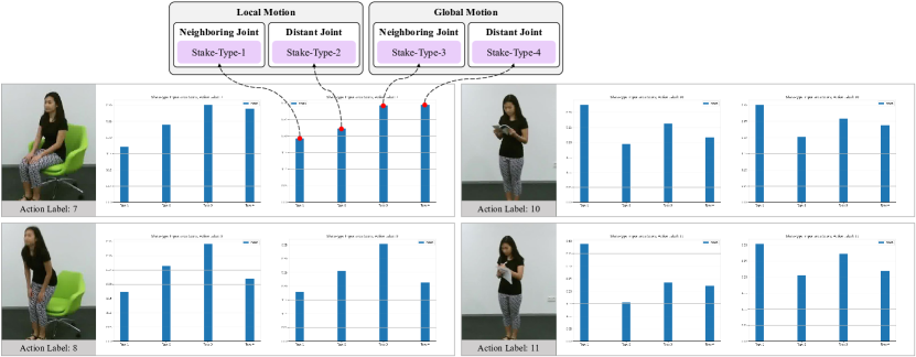
Figure 6: Skate-Type Importance Scores for various action labels.

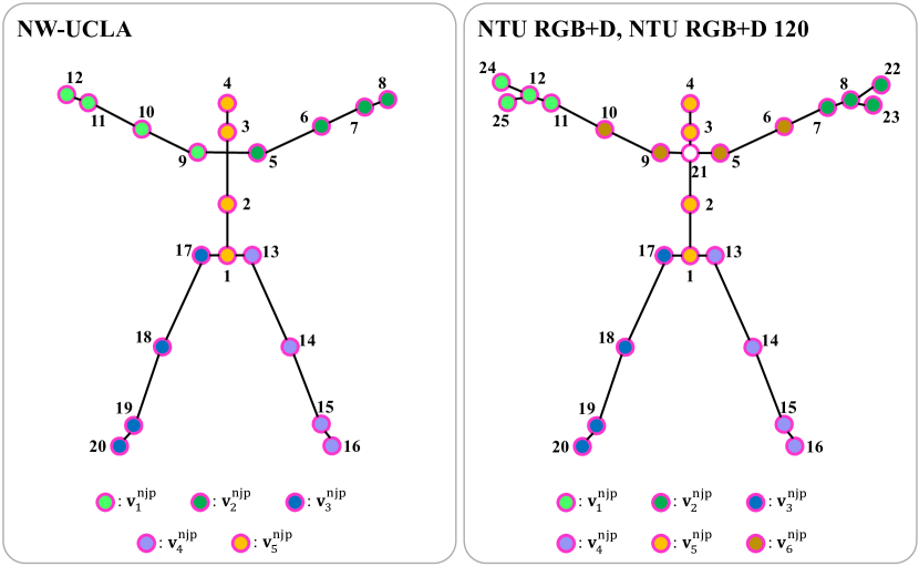
Figure 7: Skeleton tracking indices and neighboring joint partitions.

Appendix 0.C Joint Details for Various Datasets

0.C.1 Skeleton Tracking Indices and Labels of Joints

NW-UCLA. In Fig. 7, for the NW-UCLA [56] dataset acquired through the Kinect v1 [16] sensor, the skeleton of a single individual consists of a total of 20 joints. Each joint, which is a constituent unit of the skeleton, can be represented by default indices from 1 to 20, as shown in Fig. 7. The labels for each index are as follows [27]: (1) base of spine, (2) middle of spine, (3) neck, (4) head, (5) left shoulder, (6) left elbow, (7) left wrist, (8) left hand, (9) right shoulder, (10) right elbow, (11) right wrist, (12) right hand, (13) left hip, (14) left knee, (15) left ankle, (16) left foot, (17) right hip, (18) right knee, (19) right ankle, (20) right foot. We will denote joints according to their tracking indices $k$ as $v_{k}^{\mathsf{tra}}$.

NTU RGB+D and NTU RGB+D 120. In Fig. 7, for the NTU RGB+D [41] and NTU RGB+D 120 [27] datasets acquired through the Kinect v2 [16] sensor, the skeleton of a single individual consists of a total of 25 joints. These 25 joints include the original 20 joints from the Kinect v1 sensor, along with 5 additional joints representing the tips of both hands and the thumbs, as well as a spine joint. Similar to the NW-UCLA dataset, each joint can be represented by default indices from 1 to 25, as shown in Fig. 7. The labels for each index are as follows [27]: (1) base of spine, (2) middle of spine, (3) neck, (4) head, (5) left shoulder, (6) left elbow, (7) left wrist, (8) left hand, (9) right shoulder, (10) right elbow, (11) right wrist, (12) right hand, (13) left hip, (14) left knee, (15) left ankle, (16) left foot, (17) right hip, (18) right knee, (19) right ankle, (20) right foot, (21) spine, (22) tip of left hand, (23) left thumb, (24) tip of right hand, (25) right thumb.

0.C.2 Details of Neighboring Joint Partitions

In this paper, we introduce the concept of neighboring joint partitions ($\mathbf{v}_{k}^{\mathsf{njp}}$). We partitioned the entire set of joints into a total of $K$ non-overlapping subsets for our analysis. We empirically set $K$ proportional to the number of joints. We used the same number of joints for each partition since the implementation complexity was surged in usage of ‘reshaping’ and ‘attention’ functions due to the irregularity of input size. Alternative solutions as future work might be (i) reusing the same joints, (ii) trimming similar joints, or (iii) resizing the partition by linear interpolation between joints. The ordering of joints in the torso is not critical since their relative positions remain nearly constant (rigid) for any actions. We conducted experiments by varying the index order of the joints in the torso, which yielded little difference in performance. Below, we provide detailed information about the neighboring joint partitions for each dataset.

NW-UCLA. For the NW-UCLA dataset, we set $K=5$. Therefore, the total number of joints, $V=20$, is divided into $L=20/5=4$ elements, creating neighboring joint partitions. Specifically, $\mathbf{v}_{1}^{\mathsf{njp}}$ represents the joints of the right arm, $\mathbf{v}_{2}^{\mathsf{njp}}$ represents the joints of the left arm, $\mathbf{v}_{3}^{\mathsf{njp}}$ represents the joints of the right leg, $\mathbf{v}_{4}^{\mathsf{njp}}$ represents the joints of the left leg, and $\mathbf{v}_{5}^{\mathsf{njp}}$ represents the vertical torso. These partitions are ordered in a manner that extends outward from the body’s central region:

$$\begin{split}\mathbf{v}_{1}^{\mathsf{njp}}&=\left[v_{9}^{\mathsf{tra}},v_{10}^{\mathsf{tra}},v_{11}^{\mathsf{tra}},v_{12}^{\mathsf{tra}}\right]\\ \mathbf{v}_{2}^{\mathsf{njp}}&=\left[v_{5}^{\mathsf{tra}},v_{6}^{\mathsf{tra}},v_{7}^{\mathsf{tra}},v_{8}^{\mathsf{tra}}\right]\\ \mathbf{v}_{3}^{\mathsf{njp}}&=\left[v_{17}^{\mathsf{tra}},v_{18}^{\mathsf{tra}},v_{19}^{\mathsf{tra}},v_{20}^{\mathsf{tra}}\right]\\ \mathbf{v}_{4}^{\mathsf{njp}}&=\left[v_{13}^{\mathsf{tra}},v_{14}^{\mathsf{tra}},v_{15}^{\mathsf{tra}},v_{16}^{\mathsf{tra}}\right]\\ \mathbf{v}_{5}^{\mathsf{njp}}&=\left[v_{2}^{\mathsf{tra}},v_{3}^{\mathsf{tra}},v_{1}^{\mathsf{tra}},v_{4}^{\mathsf{tra}}\right].\end{split}$$ (10)

NTU RGB+D and NTU RGB+D 120. For the NTU RGB+D and NTU RGB+D 120 datasets, we set $K=12$. Since each frame in the dataset may contain up to two individuals, and to ensure accurate action recognition, we treat each individual’s joints separately. This results in a total of 50 joints per frame. In instances where only one individual is present, the remaining 25 joints are zero-padded. To facilitate partitioning, we exclude the 21st joint and consider the remaining 48 joints, resulting in $V=48$. Thus, we partition each individual’s joints into $L=48/12=4$ elements for neighboring joint partitions: $\mathbf{v}_{1}^{\mathsf{njp}}$ for the right arm, $\mathbf{v}_{2}^{\mathsf{njp}}$ for the left arm, $\mathbf{v}_{3}^{\mathsf{njp}}$ for the right leg, $\mathbf{v}_{4}^{\mathsf{njp}}$ for the left leg, $\mathbf{v}_{5}^{\mathsf{njp}}$ for the vertical torso, and $\mathbf{v}_{6}^{\mathsf{njp}}$ for the horizontal torso. These partitions are ordered in a manner that extends outward from the body’s central region:

$$\begin{split}\mathbf{v}_{1}^{\mathsf{njp}}&=\left[v_{11}^{\mathsf{tra}},v_{12}^{\mathsf{tra}},v_{24}^{\mathsf{tra}},v_{25}^{\mathsf{tra}}\right]\\ \mathbf{v}_{2}^{\mathsf{njp}}&=\left[v_{7}^{\mathsf{tra}},v_{8}^{\mathsf{tra}},v_{22}^{\mathsf{tra}},v_{23}^{\mathsf{tra}}\right]\\ \mathbf{v}_{3}^{\mathsf{njp}}&=\left[v_{17}^{\mathsf{tra}},v_{18}^{\mathsf{tra}},v_{19}^{\mathsf{tra}},v_{20}^{\mathsf{tra}}\right]\\ \mathbf{v}_{4}^{\mathsf{njp}}&=\left[v_{13}^{\mathsf{tra}},v_{14}^{\mathsf{tra}},v_{15}^{\mathsf{tra}},v_{16}^{\mathsf{tra}}\right]\\ \mathbf{v}_{5}^{\mathsf{njp}}&=\left[v_{2}^{\mathsf{tra}},v_{3}^{\mathsf{tra}},v_{1}^{\mathsf{tra}},v_{4}^{\mathsf{tra}}\right]\\ \mathbf{v}_{6}^{\mathsf{njp}}&=\left[v_{5}^{\mathsf{tra}},v_{9}^{\mathsf{tra}},v_{6}^{\mathsf{tra}},v_{10}^{\mathsf{tra}}\right].\end{split}$$ (11)

Appendix 0.D Details of Data augmentation

0.D.1 Intra-instance Augmentation

Skeletal augmentation. In our work, we employed skeletal augmentation, which includes random shear (multiply matrix $\mathsf{Sh}$ for three coordinate axes), random rotation (multiply matrix $\mathsf{R}$ for two random coordinate axes), random scaling (multiply matrix $\mathsf{Sc}$ for three coordinate axes), random skeletal flipping (swap the indices of the joints for joints with left and right pairs), random coordinate dropout (randomly remove one coordinate axis), random joint dropout (randomly remove a subset of the entire set of joints), and actor order permutation (randomly rearrange the order of actors) [14]. We did not utilize random temporal flip, random Gaussian noise, and random Gaussian blur [26] as they were found to degrade the performance of SkateFormer. Detailed information regarding the skeletal augmentation techniques employed in our study can be found in Table 11, where $p_{\mathsf{aug}}$ is application probability,

$$\mathsf{Sh}=\begin{bmatrix}1&\mathsf{sh}_{1}&\mathsf{sh}_{2}\\ \mathsf{sh}_{1}&1&\mathsf{sh}_{2}\\ \mathsf{sh}_{1}&\mathsf{sh}_{2}&1\\ \end{bmatrix},$$ (12)

$$\mathsf{R}=\begin{bmatrix}\cos\theta&-\sin\theta\\ \sin\theta&\cos\theta\\ \end{bmatrix},$$ (13)

and

$$\mathsf{Sc}=\begin{bmatrix}\mathsf{sc}_{1}&0&0\\ 0&\mathsf{sc}_{2}&0\\ 0&0&\mathsf{sc}_{3}\\ \end{bmatrix}.$$ (14)

Table 11: Details of skeletal augmentation.

Skeletal Augmentation	Hyperparameters for Each Dataset
	NW-UCLA	NTU RGB+D, NTU RGB+D 120
Random Shear	$p_{\mathsf{aug}}=0$	$p_{\mathsf{aug}}=0.5$, $\mathsf{sh}_{i}\in[-0.5,0.5]$
Random Rotation	$p_{\mathsf{aug}}=1$, $\theta\in[-\pi/3,\pi/3]$	$p_{\mathsf{aug}}=0.5$, $\theta\in[-\pi/6,\pi/6]$
Random Scaling	$p_{\mathsf{aug}}=1$, $\mathsf{sc}_{i}\in[0.5,1.5]$	$p_{\mathsf{aug}}=0.5$, $\mathsf{sc}_{i}\in[0.8,1.2]$
Random Skeletal Flipping	$p_{\mathsf{aug}}=0$	$p_{\mathsf{aug}}=0.5$
Random Coordinate Dropout	$p_{\mathsf{aug}}=0$	$p_{\mathsf{aug}}=0.5$
Random Joint Dropout	$p_{\mathsf{aug}}=0$	$p_{\mathsf{aug}}=0.5$
Actor Order Permutation	$p_{\mathsf{aug}}=0$	$p_{\mathsf{aug}}=0.5$

Temporal augmentation. Fig. 5 illustrates our trimmed-uniform random sampling of frames with $p$ portion. For this, a $p\times 100\;(0.5\leq p\leq 1)$ percentage of the total input sequence length ($T_{\mathsf{total}}$) is randomly determined before sampling. Given a $p$ value, a start-frame index $t_{s}$ is also randomly selected in the range of $0\leq t_{s}\leq\lfloor T_{\mathsf{total}}\times(1-p)\rfloor$, and the end-frame index $t_{e}$ is determined as $t_{e}=t_{s}+\lfloor T_{\mathsf{total}}\times p\rfloor$, thus constituting the selected interval $[t_{s},t_{e}]$ which is further uniformly divided into total $T$ sub-intervals. Then, as done in [12], total $T$ frames are randomly selected with one random sampling in each sub-interval. When the selected interval $[t_{s},t_{e}]$ is shorter than $T$ ($T=64$ in our case), we use linear interpolation to generate $T$ frames by a built-in PyTorch [35] function torch.nn.functional.interpolate. In the training phase, we employed a random portion $p$ (where $0.5\leq p\leq 1$) and a random start-frame index $t_{s}$ (where $0\leq t_{s}\leq\lfloor T_{\mathsf{total}}\times(1-p)\rfloor$). However, during inference, for consistency in results, we set $p=0.95$ and $t_{s}=\lfloor T_{\mathsf{total}}\times(1-p)/2\rfloor$.

Skate-Embedding. Conventional sampling methods used in generating input skeleton sequences maintain either an absolute temporal gap (i.e., the fixed stride [22, 7, 75]) or a relative temporal gap (i.e., uniform random [10, 12]) between adjacent sampled frames. Therefore, embedding temporal indices, either absolutely or relatively, using learnable features has not posed a significant challenge. However, our sampling method relies on the random variable $p$ to determine sub-intervals for sampling. Consequently, even for sequences generated from the same instance, the temporal gap between adjacent sampled frames and the sampling index of the first frame can differ significantly. This presents limitations in conveying temporal index information to the network through learnable features.

When $\lfloor T_{\mathsf{total}}\times p\rfloor\geq T$, the sampled temporal indices are designated as $t_{\mathsf{idx}}=[t_{1},t_{2},...,t_{T}]$, as illustrated in Fig 5. As mentioned, in cases of $\lfloor T_{\mathsf{total}}\times p\rfloor<T$, we perform linear interpolation across the entire index range $[t_{1},t_{2},...,t_{\lfloor T_{\mathsf{total}}\times p\rfloor}]$ to create $t_{\mathsf{idx}}=[t_{1}^{\prime},t_{2}^{\prime},...,t_{T}^{\prime}]$. The following is the detailed equation for our fixed temporal index features $\mathsf{TE}$ based on traditional sinusoidal positional embeddings [55]:

$$\begin{split}\mathsf{TE}[j,2k]&=\sin(t_{\mathsf{idx}}[j]/10000^{2k/C})\\ \mathsf{TE}[j,2k+1]&=\cos(t_{\mathsf{idx}}[j]/10000^{2k/C}),\end{split}$$ (15)

where $\mathsf{TE}\in\mathbb{R}^{T\times C}$.

0.D.2 Inter-instance Augmentation

We propose a novel inter-instance augmentation technique called Bone Length AdaIN, drawing inspiration from Skeleton AdaIN [26]. Bone Length AdaIN enhances diversity among subjects with varying body sizes by exchanging the bone lengths across different subjects in different frame sequences, rather than within each frame sequence. Detailed information on the methodology can be found in Algorithm 1. We applied inter-instance augmentation with $p_{\mathsf{aug}}=0.2$.

Algorithm 1 Bone Length AdaIN

1:Input: Input skeleton sequence $\mathbf{X}\in\mathbb{R}^{T\times V\times C_{\mathsf{in}}}$, (normalized) sampled temporal indices $\mathbf{t}_{\mathsf{idx}}\in[-1,1]^{T\times 1\times 1}$, input true label $\mathbf{y}$, entire set of skeleton sequences $\{\mathbf{X}^{n}\}_{n=1}^{N}$, and predefined adjacency matrix $\mathbf{A}$.

2:

3:Prepare reference sequence:

4:Choose the reference skeleton sequence (before sampling) $\mathbf{X}_{\mathsf{f}}^{\mathsf{b.s.}}\in\mathbb{R}^{T_{\mathsf{total},\mathsf{f}}\times V\times C_{\mathsf{in}}}$, which has same true label with $\mathbf{y}$ from $\{\mathbf{X}^{n}\}_{n=1}^{N}$.

5:Calculate the sampled temporal indices of $\mathbf{X}_{\mathsf{f}}^{\mathsf{b.s.}}$: $\mathbf{t}_{\mathsf{idx},\mathsf{f}}=\mathsf{int}((\mathbf{t}_{\mathsf{idx}}+1)/2\times T_{\mathsf{total},\mathsf{f}})\in\mathbb{N}^{T\times 1\times 1}$.

6:Sample the $\mathbf{X}_{\mathsf{f}}^{\mathsf{b.s.}}$ based on $\mathbf{t}_{\mathsf{idx},\mathsf{f}}$ (denoted as $\mathbf{X}_{\mathsf{f}}\in\mathbb{R}^{T\times V\times C_{\mathsf{in}}}$).

7:

8:Bone length calculation:

9:Calculate the bone of each skeleton sequence $\mathbf{B},\mathbf{B}_{\mathsf{f}}\in\mathbb{R}^{T\times V\times C_{\mathsf{in}}}$ from $\mathbf{X},\mathbf{X}_{\mathsf{f}}$ based on $\mathbf{A}$.

10:Calculate the bone length of each skeleton sequence $\mathbf{L},\mathbf{L}_{\mathsf{f}}\in\mathbb{R}^{T\times V\times 1}$: $\mathbf{L}=||\mathbf{B}||_{2}$ and $\mathbf{L}_{\mathsf{f}}=||\mathbf{B}_{\mathsf{f}}||_{2}$.

11:Calculate the ratio of bone length: $\mathbf{r}=(\mathbf{L}_{\mathsf{f}}+\mathsf{eps})/(\mathbf{L}+\mathsf{eps})\in\mathbb{R}^{T\times V\times 1}$, where $\mathsf{eps}=10^{-6}$.

12:

13:Bone length adaptation:

14:Adapt the bone length of input sequence: $\mathbf{B}_{\mathsf{AdaIN}}=\mathbf{B}\times\mathbf{r}$.

15:Recover the skeleton sequence (joint) $\mathbf{X}_{\mathsf{AdaIN}}$ from $\mathbf{B}_{\mathsf{AdaIN}}$ based on $\mathbf{A}$.

16:

17:Output: $\mathbf{X}_{\mathsf{AdaIN}}$

Appendix 0.E Self-Attention Analysis

0.E.1 Computational Complexity

When given the feature maps $\mathbf{Q}$, $\mathbf{K}$, and $\mathbf{V}$ of feature map $\mathbf{x}_{\mathsf{msa}}$, the computational complexity of the naive self-attention layer is $2(VT)^{2}(C/2)$:

$$\begin{split}\mathsf{Attn}=\mathsf{SoftMax}(\mathbf{Q}\mathbf{K}^{\mathsf{T}})&\rightarrow[(VT)^{2}](\frac{C}{2})\\ \mathsf{SA}(\mathbf{x}_{\mathsf{msa}})=\mathsf{Attn}\cdot\mathbf{V}&\rightarrow[(VT)\frac{C}{2}](VT),\end{split}$$ (16)

where $\mathbf{Q},\mathbf{K},\mathbf{V}\in\mathbb{R}^{(T\times V)\times C/2}$.

Let’s calculate the computation complexity for our proposed Skate-MSA. $\mathbf{x}_{\mathsf{msa}}$ is first split channel-wise ($\mathbf{x}_{\mathsf{msa}}^{i}$) and then partitioned into $\mathbf{x}_{\mathsf{msa}}^{i,\mathcal{P}}$. When considering the corresponding $\mathbf{Q}$, $\mathbf{K}$, and $\mathbf{V}$ for $\mathbf{x}_{\mathsf{msa}}^{i,\mathcal{P}}$, the computation complexity becomes $B\cdot 2(V^{\prime}T^{\prime})^{2}(C/8)$, where $\mathbf{Q},\mathbf{K},\mathbf{V}\in\mathbb{R}^{B\times(T^{\prime}\times V^{\prime})\times C/8}$. This can be easily computed in a manner similar to Eq. 16. The computation complexity for each Skate-Type is as follows:

$$\begin{split}\text{Skate-Type-1:}&(MK)\cdot 2(LN)^{2}\frac{C}{8}=2(VT)^{2}\frac{C}{2}\left[\frac{1}{4}\cdot\frac{1}{MK}\right]\\ \text{Skate-Type-2:}&(ML)\cdot 2(KN)^{2}\frac{C}{8}=2(VT)^{2}\frac{C}{2}\left[\frac{1}{4}\cdot\frac{1}{ML}\right]\\ \text{Skate-Type-3:}&(NK)\cdot 2(LM)^{2}\frac{C}{8}=2(VT)^{2}\frac{C}{2}\left[\frac{1}{4}\cdot\frac{1}{NK}\right]\\ \text{Skate-Type-4:}&(NL)\cdot 2(KM)^{2}\frac{C}{8}=2(VT)^{2}\frac{C}{2}\left[\frac{1}{4}\cdot\frac{1}{NL}\right],\end{split}$$ (17)

where $V=KL$ and $T=MN$. Therefore, by summing up all the complexities in Eq. 17, the overall complexity of Skate-MSA is as follows:

$$2(VT)^{2}\frac{C}{2}\left[\frac{1}{4}\left(\frac{1}{MK}+\frac{1}{ML}+\frac{1}{NK}+\frac{1}{NL}\right)\right].$$ (18)

Appendix 0.F Details of Implementation

0.F.1 Hyperparameters

Here is a more detailed description of the hyperparameters we used. We employed the AdamW optimizer [32] with $\beta_{1}=0.9$, $\beta_{2}=0.999$, and a weight decay value of 0.1. For the cosine-annealing scheduler [31], we set warmup learning rate to $10^{-7}$, minimum learning rate to $10^{-5}$, base learning rate to $10^{-3}$, warm-up epochs to 25, and utilized linear warm-up strategy. To prevent overfitting in the network, we set the attention map dropout ratio to 0.5 and the drop path ratio to 0.2. We did not use dropout for classification head and linear layers. The number of heads $H$ was consistent across all SkateFormer Blocks, set at 32. The expansion ratio of FFN was set to 1 for the NW-UCLA [56] dataset and 4 for the NTU RGB+D [41] and NTU RGB+D 120 [27] datasets. We employed the GELU activation function in our model.

0.F.2 Overall Architecture

The overall architecture of SkateFormer and the output shape of feature maps produced by each module are presented in Table 12.

Table 12: The details of SkateFormer.

	Mudule	Output Shape
Input		$64\times V\times 3$
Projection	$\mathsf{Linear}$ 1	$64\times V\times 6$
	$\mathsf{Linear}$ 2	$64\times V\times 9$
	$\mathsf{Linear}$ 3	$64\times V\times 96$
Stage 1	SkateFormer Block 1	$64\times V\times 96$
	SkateFormer Block 2	$64\times V\times 96$
Downsampling	$\mathsf{T{\text{-}}Conv}\;(\downarrow_{2})$ 1	$32\times V\times 96$
Stage 2	SkateFormer Block 3	$32\times V\times 192$
	SkateFormer Block 4	$32\times V\times 192$
Downsampling	$\mathsf{T{\text{-}}Conv}\;(\downarrow_{2})$ 2	$16\times V\times 192$
Stage 3	SkateFormer Block 5	$16\times V\times 192$
	SkateFormer Block 6	$16\times V\times 192$
Downsampling	$\mathsf{T{\text{-}}Conv}\;(\downarrow_{2})$ 3	$8\times V\times 192$
Stage 4	SkateFormer Block 7	$8\times V\times 192$
	SkateFormer Block 8	$8\times V\times 192$
Head	Pool	$1\times 1\times 192$
	$\mathsf{Linear}$ (classification)	$1\times 1\times N_{c}$
Output		$1\times 1\times N_{c}$

0.F.3 Modules

Details of $\mathsf{G{\text{-}}Conv}$. Let us denote $\mathbf{G}$ as learnable parameters, where $\mathbf{G}\in\mathbb{R}^{V\times V\times H/4}$. The input to $\mathsf{G{\text{-}}Conv}$, denoted as $\mathbf{x}_{\mathsf{gc}}$, is split into $H/4(=32/4=8)$ features in a channel-wise manner:

$$[\mathbf{x}_{\mathsf{gc}}^{1},...,\mathbf{x}_{\mathsf{gc}}^{H/4}]=\mathsf{Split}(\mathbf{x}_{\mathsf{gc}}),$$ (19)

where $\mathbf{x}_{\mathsf{gc}}\in\mathbb{R}^{T\times V\times C/4}$. Each $\mathbf{x}_{\mathsf{gc}}^{h}$ undergoes matrix multiplication with its corresponding $\mathbf{G}_{h}=\mathbf{G}[:,:,h]$, and the results are channel-wise concatenated to form the output of $\mathsf{G{\text{-}}Conv}$:

$$\mathsf{G{\text{-}}Conv}(\mathbf{x}_{\mathsf{gc}})=\mathsf{Concat}(\mathbf{G}_{1}\cdot\mathbf{x}_{\mathsf{gc}}^{1},...,\mathbf{G}_{H/4}\cdot\mathbf{x}_{\mathsf{gc}}^{H/4}),$$ (20)

where $\mathbf{G}_{h}\in\mathbb{R}^{V\times V}$. Through this process, we obtain an inductive bias with respect to skeletal position.

Details of FFN. The FFN of the SkateFormer Block is expressed as follows: $\mathbf{x}\leftarrow\mathbf{x}+\mathsf{Linear}(\mathsf{Act}(\mathsf{Linear}(\mathsf{LN}(\mathbf{x}))))$, where $\mathbf{x}\in\mathbb{R}^{T\times V\times C}$. If we denote the expansion ratio as $e$, the first linear layer in the FFN expands features from $C$ channels to a higher-dimensional $e\times C$ channels, and the second linear layer squeezes them back to $C$ channels from $e\times C$ channels. For the NW-UCLA dataset, we set $e=1$, while for the NTU RGB+D and NTU RGB+D 120 datasets, we used $e=4$.

Table 13: List of symbols.

	Symbol	Description
Constant	$T_{\mathsf{total}}$	The total input sequence length (Varies from one instance to another)
	$T$	The number of sampled frames ($T=64$ in our case)
	$V$	The number of total joints
	$C_{\mathsf{in}}$	The dimensionality of data representing a single joint ($C_{\mathsf{in}}=3$ in our case)
	$N_{c}$	The number of classes
Hyper- parameter	$C$	The dimensionality of feature map
	$H$	The number of total heads
	$R$	The number of total SkateFormer Blocks, $R_{1}+R_{2}+R_{3}+R_{4}$
	$K$	The number of neighboring joint partitions
	$L$	The number of distant joint partitions
	$M$	The number of local frame partitions
	$N$	The number of global frame partitions
Input	$\mathbf{X}$	Input sampled skeleton sequence ($\mathbf{X}\in\mathbb{R}^{T\times V\times C_{\mathsf{in}}}$)
	$\mathbf{f}^{t}$	$t$-th frame of input skeleton sequence ($\mathbf{f}^{t}\in\mathbb{R}^{V\times C_{\mathsf{in}}}$)
	$t_{\mathsf{idx}}$	The sampled temporal indices ($t_{\mathsf{idx}}\in\mathbb{R}^{T}$)
Output	$\hat{\mathbf{y}}$	The outcome of SkateFormer ($\hat{\mathbf{y}}\in\mathbb{R}^{N_{c}}$)
	$\mathbf{y}$	The true label ($\mathbf{y}\in\mathbb{R}^{N_{c}}$)
Skate-MSA	$\bm{\mathcal{P}}_{i}$	The $i$-th Skate-Type partition operation
	$\bm{\mathcal{R}}_{i}$	The $i$-th Skate-Type reverse operation
	$\mathbf{v}$	The skeletal axis of feature map $\mathbf{x}$
	$\mathbf{t}$	The time axis of feature map $\mathbf{x}$
	$\mathbf{v}_{k}^{\mathsf{njp}}$	The $k$-th neighboring joint partition, $\mathbf{v}=\{\mathbf{v}_{k}^{\mathsf{njp}}\}_{k=1}^{K}$
	$\mathbf{v}_{l}^{\mathsf{djp}}$	The $l$-th distant joint partition, $\mathbf{v}=\{\mathbf{v}_{l}^{\mathsf{djp}}\}_{l=1}^{L}$
	$\mathbf{t}_{m}^{\mathsf{local}}$	The $m$-th local frame partition, $\mathbf{t}=\{\mathbf{t}_{m}^{\mathsf{local}}\}_{m=1}^{M}$
	$\mathbf{t}_{n}^{\mathsf{global}}$	The $n$-th global frame partition, $\mathbf{t}=\{\mathbf{t}_{n}^{\mathsf{global}}\}_{n=1}^{N}$
Feature	$\mathbf{x}$	The input for SkateFormer Block ($\mathbf{x}\in\mathbb{R}^{T\times V\times C}$)
	$\mathbf{x}_{\mathsf{gc}}$	The input for $\mathsf{G{\text{-}}Conv}$ ($\mathbf{x}_{\mathsf{gc}}\in\mathbb{R}^{T\times V\times\frac{C}{4}}$)
	$\mathbf{x}_{\mathsf{tc}}$	The input for $\mathsf{T{\text{-}}Conv}$ ($\mathbf{x}_{\mathsf{tc}}\in\mathbb{R}^{T\times V\times\frac{C}{4}}$)
	$\mathbf{x}_{\mathsf{msa}}$	The input for Skate-MSA ($\mathbf{x}_{\mathsf{msa}}\in\mathbb{R}^{T\times V\times\frac{C}{2}}$)
	$\mathbf{x}_{\mathsf{msa}}^{i}$	The input for MSA of $i$-th Skate-Type ($\mathbf{x}_{\mathsf{msa}}^{i}\in\mathbb{R}^{T\times V\times\frac{C}{8}}$)
	$\mathbf{x}_{\mathsf{msa}}^{i,\bm{\mathcal{P}}}$	The partitioned $\mathbf{x}_{\mathsf{msa}}^{i}$, $\bm{\mathcal{P}}_{i}(\mathbf{x}_{\mathsf{msa}}^{i})$

References

- [1] Cai, D., Kang, Y., Yao, A., Chen, Y.: Ske2grid: Skeleton-to-grid representation learning for action recognition. In: International Conference on Machine Learning (2023)
- [2] Cao, Z., Simon, T., Wei, S.E., Sheikh, Y.: Realtime multi-person 2d pose estimation using part affinity fields. In: Proceedings of the IEEE conference on computer vision and pattern recognition. pp. 7291–7299 (2017)
- [3] Chen, Y., Zhang, Z., Yuan, C., Li, B., Deng, Y., Hu, W.: Channel-wise topology refinement graph convolution for skeleton-based action recognition. In: Proceedings of the IEEE/CVF international conference on computer vision. pp. 13359–13368 (2021)
- [4] Chen, Z., Li, S., Yang, B., Li, Q., Liu, H.: Multi-scale spatial temporal graph convolutional network for skeleton-based action recognition. In: Proceedings of the AAAI conference on artificial intelligence. vol. 35, pp. 1113–1122 (2021)
- [5] Cheng, K., Zhang, Y., Cao, C., Shi, L., Cheng, J., Lu, H.: Decoupling gcn with dropgraph module for skeleton-based action recognition. In: Computer Vision–ECCV 2020: 16th European Conference, Glasgow, UK, August 23–28, 2020, Proceedings, Part XXIV 16. pp. 536–553. Springer (2020)
- [6] Cheng, K., Zhang, Y., He, X., Chen, W., Cheng, J., Lu, H.: Skeleton-based action recognition with shift graph convolutional network. In: Proceedings of the IEEE/CVF conference on computer vision and pattern recognition. pp. 183–192 (2020)
- [7] Chi, H.g., Ha, M.H., Chi, S., Lee, S.W., Huang, Q., Ramani, K.: Infogcn: Representation learning for human skeleton-based action recognition. In: Proceedings of the IEEE/CVF Conference on Computer Vision and Pattern Recognition. pp. 20186–20196 (2022)
- [8] Ding, Z., Wang, P., Ogunbona, P.O., Li, W.: Investigation of different skeleton features for cnn-based 3d action recognition. In: 2017 IEEE International conference on multimedia & expo workshops (ICMEW). pp. 617–622. IEEE (2017)
- [9] Dosovitskiy, A., Beyer, L., Kolesnikov, A., Weissenborn, D., Zhai, X., Unterthiner, T., Dehghani, M., Minderer, M., Heigold, G., Gelly, S., et al.: An image is worth 16x16 words: Transformers for image recognition at scale. arXiv preprint arXiv:2010.11929 (2020)
- [10] Duan, H., Wang, J., Chen, K., Lin, D.: Pyskl: Towards good practices for skeleton action recognition. In: Proceedings of the 30th ACM International Conference on Multimedia. pp. 7351–7354 (2022)
- [11] Duan, H., Xu, M., Shuai, B., Modolo, D., Tu, Z., Tighe, J., Bergamo, A.: Skeletr: Towards skeleton-based action recognition in the wild. In: Proceedings of the IEEE/CVF International Conference on Computer Vision. pp. 13634–13644 (2023)
- [12] Duan, H., Zhao, Y., Chen, K., Lin, D., Dai, B.: Revisiting skeleton-based action recognition. In: Proceedings of the IEEE/CVF Conference on Computer Vision and Pattern Recognition. pp. 2969–2978 (2022)
- [13] Gao, Z., Wang, P., Lv, P., Jiang, X., Liu, Q., Wang, P., Xu, M., Li, W.: Focal and global spatial-temporal transformer for skeleton-based action recognition. In: Proceedings of the Asian Conference on Computer Vision. pp. 382–398 (2022)
- [14] Guo, T., Liu, H., Chen, Z., Liu, M., Wang, T., Ding, R.: Contrastive learning from extremely augmented skeleton sequences for self-supervised action recognition. In: Proceedings of the AAAI Conference on Artificial Intelligence. vol. 36, pp. 762–770 (2022)
- [15] Ilg, E., Mayer, N., Saikia, T., Keuper, M., Dosovitskiy, A., Brox, T.: Flownet 2.0: Evolution of optical flow estimation with deep networks. In: Proceedings of the IEEE conference on computer vision and pattern recognition. pp. 2462–2470 (2017)
- [16] Kay, W., Carreira, J., Simonyan, K., Zhang, B., Hillier, C., Vijayanarasimhan, S., Viola, F., Green, T., Back, T., Natsev, P., et al.: The kinetics human action video dataset. arXiv preprint arXiv:1705.06950 (2017)
- [17] Ke, Q., Bennamoun, M., An, S., Sohel, F., Boussaid, F.: Learning clip representations for skeleton-based 3d action recognition. IEEE Transactions on Image Processing 27(6), 2842–2855 (2018)
- [18] Kipf, T.N., Welling, M.: Semi-supervised classification with graph convolutional networks. arXiv preprint arXiv:1609.02907 (2016)
- [19] Korban, M., Li, X.: Ddgcn: A dynamic directed graph convolutional network for action recognition. In: Computer Vision–ECCV 2020: 16th European Conference, Glasgow, UK, August 23–28, 2020, Proceedings, Part XX 16. pp. 761–776. Springer (2020)
- [20] Kwon, T., Tekin, B., Stühmer, J., Bogo, F., Pollefeys, M.: H2o: Two hands manipulating objects for first person interaction recognition. In: Proceedings of the IEEE/CVF International Conference on Computer Vision. pp. 10138–10148 (2021)
- [21] Lee, J., Lee, M., Cho, S., Woo, S., Jang, S., Lee, S.: Leveraging spatio-temporal dependency for skeleton-based action recognition. In: Proceedings of the IEEE/CVF International Conference on Computer Vision. pp. 10255–10264 (2023)
- [22] Lee, J., Lee, M., Lee, D., Lee, S.: Hierarchically decomposed graph convolutional networks for skeleton-based action recognition. In: Proceedings of the IEEE/CVF International Conference on Computer Vision. pp. 10444–10453 (2023)
- [23] Li, B., Dai, Y., Cheng, X., Chen, H., Lin, Y., He, M.: Skeleton based action recognition using translation-scale invariant image mapping and multi-scale deep cnn. In: 2017 IEEE International Conference on Multimedia & Expo Workshops (ICMEW). pp. 601–604. IEEE (2017)
- [24] Li, M., Chen, S., Chen, X., Zhang, Y., Wang, Y., Tian, Q.: Actional-structural graph convolutional networks for skeleton-based action recognition. In: Proceedings of the IEEE/CVF conference on computer vision and pattern recognition. pp. 3595–3603 (2019)
- [25] Li, S., Li, W., Cook, C., Zhu, C., Gao, Y.: Independently recurrent neural network (indrnn): Building a longer and deeper rnn. In: Proceedings of the IEEE conference on computer vision and pattern recognition. pp. 5457–5466 (2018)
- [26] Lin, L., Zhang, J., Liu, J.: Actionlet-dependent contrastive learning for unsupervised skeleton-based action recognition. In: Proceedings of the IEEE/CVF Conference on Computer Vision and Pattern Recognition. pp. 2363–2372 (2023)
- [27] Liu, J., Shahroudy, A., Perez, M., Wang, G., Duan, L.Y., Kot, A.C.: Ntu rgb+ d 120: A large-scale benchmark for 3d human activity understanding. IEEE transactions on pattern analysis and machine intelligence 42(10), 2684–2701 (2019)
- [28] Liu, J., Shahroudy, A., Xu, D., Wang, G.: Spatio-temporal lstm with trust gates for 3d human action recognition. In: Computer Vision–ECCV 2016: 14th European Conference, Amsterdam, The Netherlands, October 11-14, 2016, Proceedings, Part III 14. pp. 816–833. Springer (2016)
- [29] Liu, J., Wang, G., Duan, L.Y., Abdiyeva, K., Kot, A.C.: Skeleton-based human action recognition with global context-aware attention lstm networks. IEEE Transactions on Image Processing 27(4), 1586–1599 (2017)
- [30] Liu, Z., Lin, Y., Cao, Y., Hu, H., Wei, Y., Zhang, Z., Lin, S., Guo, B.: Swin transformer: Hierarchical vision transformer using shifted windows. In: Proceedings of the IEEE/CVF international conference on computer vision. pp. 10012–10022 (2021)
- [31] Loshchilov, I., Hutter, F.: Sgdr: Stochastic gradient descent with warm restarts. arXiv preprint arXiv:1608.03983 (2016)
- [32] Loshchilov, I., Hutter, F.: Decoupled weight decay regularization. arXiv preprint arXiv:1711.05101 (2017)
- [33] Müller, R., Kornblith, S., Hinton, G.E.: When does label smoothing help? Advances in neural information processing systems 32 (2019)
- [34] Pang, Y., Ke, Q., Rahmani, H., Bailey, J., Liu, J.: Igformer: Interaction graph transformer for skeleton-based human interaction recognition. In: European Conference on Computer Vision. pp. 605–622. Springer (2022)
- [35] Paszke, A., Gross, S., Chintala, S., Chanan, G., Yang, E., DeVito, Z., Lin, Z., Desmaison, A., Antiga, L., Lerer, A.: Automatic differentiation in pytorch (2017)
- [36] Peng, W., Hong, X., Chen, H., Zhao, G.: Learning graph convolutional network for skeleton-based human action recognition by neural searching. In: Proceedings of the AAAI conference on artificial intelligence. vol. 34, pp. 2669–2676 (2020)
- [37] Perez, M., Liu, J., Kot, A.C.: Interaction relational network for mutual action recognition. IEEE Transactions on Multimedia 24, 366–376 (2021)
- [38] Plizzari, C., Cannici, M., Matteucci, M.: Skeleton-based action recognition via spatial and temporal transformer networks. Computer Vision and Image Understanding 208, 103219 (2021)
- [39] Presti, L.L., La Cascia, M.: 3d skeleton-based human action classification: A survey. Pattern Recognition 53, 130–147 (2016)
- [40] Qiu, H., Hou, B., Ren, B., Zhang, X.: Spatio-temporal segments attention for skeleton-based action recognition. Neurocomputing 518, 30–38 (2023)
- [41] Shahroudy, A., Liu, J., Ng, T.T., Wang, G.: Ntu rgb+ d: A large scale dataset for 3d human activity analysis. In: Proceedings of the IEEE conference on computer vision and pattern recognition. pp. 1010–1019 (2016)
- [42] Shi, L., Zhang, Y., Cheng, J., Lu, H.: Skeleton-based action recognition with directed graph neural networks. In: Proceedings of the IEEE/CVF conference on computer vision and pattern recognition. pp. 7912–7921 (2019)
- [43] Shi, L., Zhang, Y., Cheng, J., Lu, H.: Two-stream adaptive graph convolutional networks for skeleton-based action recognition. In: Proceedings of the IEEE/CVF conference on computer vision and pattern recognition. pp. 12026–12035 (2019)
- [44] Shi, L., Zhang, Y., Cheng, J., Lu, H.: Decoupled spatial-temporal attention network for skeleton-based action-gesture recognition. In: Proceedings of the Asian Conference on Computer Vision (2020)
- [45] Si, C., Chen, W., Wang, W., Wang, L., Tan, T.: An attention enhanced graph convolutional lstm network for skeleton-based action recognition. In: Proceedings of the IEEE/CVF conference on computer vision and pattern recognition. pp. 1227–1236 (2019)
- [46] Song, Y.F., Zhang, Z., Shan, C., Wang, L.: Stronger, faster and more explainable: A graph convolutional baseline for skeleton-based action recognition. In: proceedings of the 28th ACM international conference on multimedia. pp. 1625–1633 (2020)
- [47] Song, Y.F., Zhang, Z., Shan, C., Wang, L.: Constructing stronger and faster baselines for skeleton-based action recognition. IEEE transactions on pattern analysis and machine intelligence 45(2), 1474–1488 (2022)
- [48] Sovrasov, V.: ptflops: a flops counting tool for neural networks in pytorch framework (2018–2023), https://github.com/sovrasov/flops-counter.pytorch
- [49] Sun, D., Yang, X., Liu, M.Y., Kautz, J.: Pwc-net: Cnns for optical flow using pyramid, warping, and cost volume. In: Proceedings of the IEEE conference on computer vision and pattern recognition. pp. 8934–8943 (2018)
- [50] Sun, K., Xiao, B., Liu, D., Wang, J.: Deep high-resolution representation learning for human pose estimation. In: Proceedings of the IEEE/CVF conference on computer vision and pattern recognition. pp. 5693–5703 (2019)
- [51] Sun, Z., Ke, Q., Rahmani, H., Bennamoun, M., Wang, G., Liu, J.: Human action recognition from various data modalities: A review. IEEE transactions on pattern analysis and machine intelligence (2022)
- [52] Szegedy, C., Vanhoucke, V., Ioffe, S., Shlens, J., Wojna, Z.: Rethinking the inception architecture for computer vision. In: Proceedings of the IEEE conference on computer vision and pattern recognition. pp. 2818–2826 (2016)
- [53] Tu, Z., Talebi, H., Zhang, H., Yang, F., Milanfar, P., Bovik, A., Li, Y.: Maxim: Multi-axis mlp for image processing. In: Proceedings of the IEEE/CVF Conference on Computer Vision and Pattern Recognition. pp. 5769–5780 (2022)
- [54] Tu, Z., Talebi, H., Zhang, H., Yang, F., Milanfar, P., Bovik, A., Li, Y.: Maxvit: Multi-axis vision transformer. In: European conference on computer vision. pp. 459–479. Springer (2022)
- [55] Vaswani, A., Shazeer, N., Parmar, N., Uszkoreit, J., Jones, L., Gomez, A.N., Kaiser, Ł., Polosukhin, I.: Attention is all you need. Advances in neural information processing systems 30 (2017)
- [56] Wang, J., Nie, X., Xia, Y., Wu, Y., Zhu, S.C.: Cross-view action modeling, learning and recognition. In: Proceedings of the IEEE conference on computer vision and pattern recognition. pp. 2649–2656 (2014)
- [57] Wang, L., Huynh, D.Q., Koniusz, P.: A comparative review of recent kinect-based action recognition algorithms. IEEE Transactions on Image Processing 29, 15–28 (2019)
- [58] Wang, L., Koniusz, P.: 3mformer: Multi-order multi-mode transformer for skeletal action recognition. In: Proceedings of the IEEE/CVF Conference on Computer Vision and Pattern Recognition. pp. 5620–5631 (2023)
- [59] Wang, P., Li, Z., Hou, Y., Li, W.: Action recognition based on joint trajectory maps using convolutional neural networks. In: Proceedings of the 24th ACM international conference on Multimedia. pp. 102–106 (2016)
- [60] Wang, Q., Shi, S., He, J., Peng, J., Liu, T., Weng, R.: Iip-transformer: Intra-inter-part transformer for skeleton-based action recognition. In: 2023 IEEE International Conference on Big Data (BigData). pp. 936–945. IEEE (2023)
- [61] Wang, X., Xu, X., Mu, Y.: Neural koopman pooling: Control-inspired temporal dynamics encoding for skeleton-based action recognition. In: Proceedings of the IEEE/CVF Conference on Computer Vision and Pattern Recognition. pp. 10597–10607 (2023)
- [62] Wen, Y., Tang, Z., Pang, Y., Ding, B., Liu, M.: Interactive spatiotemporal token attention network for skeleton-based general interactive action recognition. In: 2023 IEEE/RSJ International Conference on Intelligent Robots and Systems (IROS). pp. 7886–7892. IEEE (2023)
- [63] Xiang, W., Li, C., Zhou, Y., Wang, B., Zhang, L.: Generative action description prompts for skeleton-based action recognition. In: Proceedings of the IEEE/CVF International Conference on Computer Vision. pp. 10276–10285 (2023)
- [64] Xin, W., Miao, Q., Liu, Y., Liu, R., Pun, C.M., Shi, C.: Skeleton mixformer: Multivariate topology representation for skeleton-based action recognition. In: Proceedings of the 31st ACM International Conference on Multimedia. pp. 2211–2220 (2023)
- [65] Xu, K., Ye, F., Zhong, Q., Xie, D.: Topology-aware convolutional neural network for efficient skeleton-based action recognition. In: Proceedings of the AAAI Conference on Artificial Intelligence. vol. 36, pp. 2866–2874 (2022)
- [66] Xu, Y., Cheng, J., Wang, L., Xia, H., Liu, F., Tao, D.: Ensemble one-dimensional convolution neural networks for skeleton-based action recognition. IEEE Signal Processing Letters 25(7), 1044–1048 (2018)
- [67] Yan, S., Xiong, Y., Lin, D.: Spatial temporal graph convolutional networks for skeleton-based action recognition. In: Proceedings of the AAAI conference on artificial intelligence. vol. 32 (2018)
- [68] Ye, F., Pu, S., Zhong, Q., Li, C., Xie, D., Tang, H.: Dynamic gcn: Context-enriched topology learning for skeleton-based action recognition. In: Proceedings of the 28th ACM international conference on multimedia. pp. 55–63 (2020)
- [69] Zeng, A., Sun, X., Yang, L., Zhao, N., Liu, M., Xu, Q.: Learning skeletal graph neural networks for hard 3d pose estimation. In: Proceedings of the IEEE/CVF international conference on computer vision. pp. 11436–11445 (2021)
- [70] Zhang, J., He, T., Sra, S., Jadbabaie, A.: Why gradient clipping accelerates training: A theoretical justification for adaptivity. arXiv preprint arXiv:1905.11881 (2019)
- [71] Zhang, P., Lan, C., Xing, J., Zeng, W., Xue, J., Zheng, N.: View adaptive recurrent neural networks for high performance human action recognition from skeleton data. In: Proceedings of the IEEE international conference on computer vision. pp. 2117–2126 (2017)
- [72] Zhang, P., Lan, C., Zeng, W., Xing, J., Xue, J., Zheng, N.: Semantics-guided neural networks for efficient skeleton-based human action recognition. In: proceedings of the IEEE/CVF conference on computer vision and pattern recognition. pp. 1112–1121 (2020)
- [73] Zhang, Y., Wu, B., Li, W., Duan, L., Gan, C.: Stst: Spatial-temporal specialized transformer for skeleton-based action recognition. In: Proceedings of the 29th ACM International Conference on Multimedia. pp. 3229–3237 (2021)
- [74] Zhang, Z.: Microsoft kinect sensor and its effect. IEEE multimedia 19(2), 4–10 (2012)
- [75] Zhou, H., Liu, Q., Wang, Y.: Learning discriminative representations for skeleton based action recognition. In: Proceedings of the IEEE/CVF Conference on Computer Vision and Pattern Recognition. pp. 10608–10617 (2023)
- [76] Zhou, Y., Li, C., Cheng, Z.Q., Geng, Y., Xie, X., Keuper, M.: Hypergraph transformer for skeleton-based action recognition. arXiv preprint arXiv:2211.09590 (2022)
- [77] Zhu, W., Lan, C., Xing, J., Zeng, W., Li, Y., Shen, L., Xie, X.: Co-occurrence feature learning for skeleton based action recognition using regularized deep lstm networks. In: Proceedings of the AAAI conference on artificial intelligence. vol. 30 (2016)